User’s GuideVersion 4

Contents

• Introduction

• MATH-TEACHER PLUS series

• Tutorial Program For Student

• Exploration Environment

• The Curriculum

• Teachers’ Toolkit

• Technical Information

© Copyright 2004 Hickerson Education, Inc.

Customer Support Hickerson Education wants to resolve any problem you have. Contact us by:

Phone: US and Canada: 4:20 Communications 763-323-8257Phone: Orders: 888-MATHKAL Fax: 763-323-8222E-Mail: info@mathkalusa.comhttp://www.mathkalusa.com

INTRODUCTIONLearning Math at your own paceIs the key to Math success!

This is the motto that Math-Kal has put on its banner since its foundation in 1992. The company wasestablished by a group of experienced mathematics teachers. After many years of working with students,they had the vision of using the computer as a helpful tool for individual progress in mathematics.

Mathematics instruction has several facets, such as understanding concepts, discovery, mastering skills,applying theorems, proving theorems and mathematical facts. Math-Kal provides a unique interactivetool, MATH-TEACHER PLUS, that allows students to master skills and concepts and fully understandthe ideas behind the concepts taught in the classroom. It consists of a highly interactive tutorial programand an open-ended tool, the exploration environment. The exploration environment allows students toexplore and investigate mathematical phenomena by themselves, or with the help of their teachers. Theexploration environment somewhat resembles an advanced graphic calculator, with a lot more power.

The mastering skills process is extremely interactive. A problem is presented to the student who mustprovide an answer, which is not necessarily the final one. The program leads the student to the finalanswer by providing guidance, hints and comments on each step of the solving process. In addition, theprogram includes lessons, accompanied by many examples in each of the topics, for those who need torefresh their memory. It also includes timed on-line tests that can be used for self-checking, as well as anevaluating tool for the teacher. All the student’s activities and grades, are collected and a detailedindividual report is generated. It can be printed out at the end of the session, or kept in a database. Thereport also includes statistics on how many hints and guidance messages the student used, and otherindications of their performance.

The combination of the open ended tool and the interactive tutorial sessions forms a unique math learningenvironment that ensures efficient and enjoyable math learning.

MATH-TEACHER PLUS series includes toolkit for teachers. It combines three useful utilities forteachers: Printed Tests Generator, Customization Program and Student Management System.The toolkit provides a supportive teaching environment for teachers, it helps them instruct better andeases the preparations for their instructural tasks.

MATH-TEACHER PLUS programs cover the major part of the curriculum of junior high school, highschool and the first year of college. The software is user-friendly and simple to operate. With all itsunique features, MATH-TEACHER PLUS is a powerful tool, both for students and teachers.

Students love it, teachers appreciate it!!

Chapter 1: MATH-TEACHER PLUS Series1.1 Available PackagesMath-Kal offers products for students that enable them mastering skills in mathematics and help themunderstand concepts, ideas and phenomena. It also offers tools for teachers to ease their daily work asinstructors.Each one of the products is a collection of four units. A unit covers material that is usually taught in classover a period of 2-4 months, depending on the subject and the ability of the students.The products are:•••• Algebra 1•••• Algebra 2•••• Word Problems and Probability•••• Coordinate Geometry and Trigonometry•••• Calculus and Linear Programming

Algebra 1 • Algebraic Expressions - First Steps Substitution in expressions, operations on expressions, building expressions, factorization • Algebraic Expressions - Intermediate Special products, factorization, building equations, integer and rational exponentiation, rational

expressions • Area and Volume The Metric system, calculations of area and volume • Equations and Inequalities of the First Degree Equations and inequalities of the first degree with one variable

Algebra 2 • Equations and Inequalities of the Second Degree Equations and inequalities of the second degree with one variable • Equations and Systems with Two Variables Linear equations and systems with two variables • Quadratic System and Parameters Quadratic systems, linear equations and systems with a parameter • Sequences Explicit and recursive definition, arithmetic and geometric progression

Word Problems and Probability • Problems on Percentages and Numbers First degree problems in percentages and numbers • Problems on Geometric Shapes and Motion Problems of the first degree dealing with geometrical shapes and uniform motion • Probability - Calculations Calculation of probabilities, conditional probability, tree diagrams • Probability - Combinatorics and Distributions Combinatorics, binomial and normal distributions

Coordinate Geometry and Trigonometry

• Coordinate Geometry - Points, Line, Circle Points in the plane, the straight line, the circle • Coordinate Geometry - Ellipse, Hyperbola, Parabola The ellipse, the hyperbola, the parabola • Trigonometry of the Triangle Definition of the trigonometric functions, solving triangles and shapes • Advanced Trigonometry Extension of functions to the real line, trigonometric identities and equations

Calculus and Linear Programming • Calculus - Derivative of Polynomials The notion of the derivative, investigating polynomial functions • Calculus - Derivative of Elementary Functions Deriving and investigating elementary functions • Calculus - Integrals Antiderivatives, calculation of area and volume • Linear Programming Systems of inequalities with two variables, solving problems

1.2 Package ContentEach package consists of two basic programs: • Tutorial program for students

• Toolkit for teachers

The tutorial program allows students to read lessons, solve problems interactively, test their skills bytimed online tests and explore mathematical phenomena.

The toolkit program consists of three utilities: • Customization Utility

• Printed Tests Generator

• Student Management System

The Customization Utility helps teachers to fine-tune the tutorial program. Using this utility, the teachercan set a number of parameters that control the way that MATH-TEACHER PLUS programs operate. Forexample, the number of problems that the student is required to solve before proceeding to the next level.Default values have already been set, therefore teachers would run this utility only if different values areneeded. Adaptations need to be specified prior to the beginning of a student’s working session.

The Printed Tests Generator is used by teachers to printout tests or homework. Each printout includes aset of problems and optionally the answers, showing the working steps of the solution. While building thetest, teachers can determine the number of problems on each subject and each level that will be printedout. This is a useful tool as the teacher can print out different lists for each student, hand them out ashomework or test, and finally give the detailed answers to the students for self-check.

Student Management System is the utility that helps teachers to keep track of students work in the lab.Students' records are saved in a database and can be retrieved later for printing reports.These records can be handled as individual student records or as class records.

Various options of statistics are available, and hard copies of the reports can be printed out.

1.3 MediaMATH-TEACHER PLUS products are available for schools as a site license for a network andstand-alone machines, or lab pack (5 CDs). It is also available on CD for individuals, home-schoolers andother students and teachers.

1.4 Target AudienceThe broad curriculum of MATH-TEACHER PLUS is targeted at junior and senior high school students,normally in grades 7-12, students in their first years of college and adults.

Chapter 2: Tutorial Program for Students

2.1 General StructureMATH-TEACHER PLUS is built hierarchically.The basic building block is called a unit which covers mathematical material of 2-6 weeks in school.Each unit consists of between two and five subjects.

The software provides three learning activities for each subject: • Lesson - an electronic textbook which explains the theories and comes with examples • Interactive Tutorial – hands on practice, allows skills mastering • Test - on-line timed test for assessment

All the panels are built along general guidelines: • The top bar indicates the panel title • The left bar includes operational buttons • Any button that can be clicked has a pointing finger cursor • Each panel has a help button. Once this button is clicked the cursor changes to question mark.

Clicking objects on the panel displays the help associated with the objects.

2.2 Opening Panel and Units PanelIn the main opening panel, the student is required to fill personal data. It includes the student's name,class ID and personal password if SMS (Student Management System) is installed. The last two items aregiven to students by the system administrator.

Once the student clicks OK, the units panel is presented on the screen. This panel contains the units thatare installed in the system. For example, if a school purchased the product Algebra-1 the following fourunits will be presented:

• Algebraic Expressions - First Steps • Algebraic Expressions - Intermediate • Area and Volume • Equations and Inequalities of the First Degree

If a school has purchased site license of all the products, all 20 units will be available.

Subject Interactive Tutorial:consists of Levels

Lesson:consists of Sections

Test:consists of Levels

Unit

The units are organized as follows: ! Algebraic Expressions (two units) ! Area and Volume ! Equations (four units) ! Word Problems (two units) ! Linear Programming ! Sequences ! Coordinate Geometry (two units) ! Trigonometry (two units) ! Calculus (three units) ! Probability (two units)

The syllabus button enables you to access the content of MATH-TEACHER Plus from a different path.Once you click this button, a list of textbooks and syllabus of various courses is displayed. You can clicka specific textbook's name; The titles of the chapters and sections in this book are displayed, enabling youto get directly to a specific tutorial part correlated to any specific chapter in the book.One of the items in the list, is the curriculum of MATH-TEACHER Plus; It is organized as a list ofmathematical topics from which you can access directly the interactive tutorial section. It means that youdo not have to work through the regular format of choosing a unit, then a subject and finally a level.

The bookmark is an important feature of the program. The system keeps track of the student's workingstatus by marking a bookmark in the database. The bookmark contains information about the unit, subjectand level of tutorial session.If a student leaves the session in the middle of a level, the program bookmarks this place and he/sheautomatically begins in this place the next time the student logs on. For example, a student that started topractice at a certain level, and completed 3 problems out of 5, is enabled, by the bookmark mechanism, to

get directly to the unit-subject-level status where he/she stopped. Now the student need only solve twomore problems to complete the activity.Exiting the tutorial program during a test does not keep a bookmark automatically, as it does with theinteractive tutorial. Since all problems were already presented to the student, there is no point allowinghim/her to get back to the same test.

Note: The bookmark feature is applicable only when SMS (Student Management System) isinstalled.

Click one of the buttons to pass to the unit panel.

2.3 Unit PanelThis panel is organized as a matrix in which the rows represent the subjects of the unit, and the columnsare the learning activities: “Lesson”, “Interactive Tutorial” and “Test”.The following panel shows the unit panel of "Algebraic Expressions - Intermediate".

To start any of these activities, click the corresponding entry of the matrix.Each click opens an internal panel with the relevant information:Clicking an entry of the matrix in the lesson column displays the list of sections of that subject. Select oneof the sections to pass to the lesson panel.Clicking an entry of the matrix in the tutorial column displays the list of levels of that subject. Select oneof the levels to pass to the tutorial panel.Clicking an entry of the matrix in the test column displays the test information. Click the test button topass to the test panel.

2.4 Lesson PanelThe lesson panel consists mostly of three sub-windows: Theory, example and optionally graphics ortables. The lesson of each subject is made up of sections. The lesson panel displays one section at a time.The example below shows the lesson panel of the unit "Calculus - Derivative of Polynomials", in thesubject "Investigating Polynomials".

The theory part describes the mathematical concepts in the section. Mostly, it is accompanied bysub-window displaying an example related to the content of the section.

Note: The lesson panel consists of theoretical material and examples.The theory is written in the section sub-window and you can view many examples that demonstrate theconcepts described in the section. The examples are accompanied with graphics and tables if needed. Ifnone is needed, a picture of a well-known mathematician is displayed. Each example describes a problemor exercise and all the steps of the solution.

Note: Each example is different.Click “Example” to view a different example. You can click “Example” as many times as you wish: youwill always see a new example. Like the mechanism that produces problems for practice purposes, thealgorithm that generates examples produces a different one each time. Practically, an infinite number ofexamples are available on each level, since they are not taken from a certain pre-defined database ofproblems, but rather are generated randomly.

Note: The examples get more and more difficult.When you start viewing a section in a lesson, the first example shown is the simplest possible. As youview more examples, they become more and more complex. After they reach the highest degree ofcomplexity in this level, they will go back to the simplest kind in this level.

Note: The lesson is a tool that helps you to review material.You can review the various sections related to the current subject. You can access the lesson panel whileyou are solving problems from the interactive tutorial panel or before you start the practice phase.

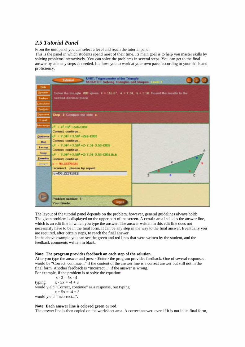
2.5 Tutorial PanelFrom the unit panel you can select a level and reach the tutorial panel.This is the panel in which students spend most of their time. Its main goal is to help you master skills bysolving problems interactively. You can solve the problems in several steps. You can get to the finalanswer by as many steps as needed. It allows you to work at your own pace, according to your skills andproficiency.

The layout of the tutorial panel depends on the problem, however, general guidelines always hold:The given problem is displayed on the upper part of the screen. A certain area includes the answer line,which is an edit line in which you type the answer. The answer written in this edit line does notnecessarily have to be in the final form. It can be any step in the way to the final answer. Eventually youare required, after certain steps, to reach the final answer.In the above example you can see the green and red lines that were written by the student, and thefeedback comments written in black.

Note: The program provides feedback on each step of the solution.After you type the answer and press <Enter> the program provides feedback. One of several responseswould be “Correct, continue...” if the content of the answer line is a correct answer but still not in thefinal form. Another feedback is “Incorrect...” if the answer is wrong.For example, if the problem is to solve the equation: x - 3 = 5x - 4typing x - 5x = -4 + 3would yield “Correct, continue” as a response, but typing x + 5x = -4 + 3would yield "Incorrect...".

Note: Each answer line is colored green or red.The answer line is then copied on the worksheet area. A correct answer, even if it is not in its final form,

is colored green. An incorrect answer is colored red. Each time an answer line is colored (red or green) anew answer line appears in the worksheet area. There is no way to change the previous answer lines.

Tip: You can make up to three mistakes during the solution process.The solution process may require several steps and each student may need a different number of steps.You can type many correct steps, however, each mistake is counted and a total of up to three is allowedper question. If you make three mistakes all steps of the answer will automatically be displayed.

Tip: Syntax error is not counted.The program alerts when a syntax error is made by a special message.For example, typing: x - 5x = -4 +would yield a “syntax error” because the expression is illegal.If you make a syntax error you can re-edit the line and fix your error.

Tip: Any answer that is mathematically correct is accepted and colored green.For example, in the process of solving an equation, you can type a set of equivalent equations until youreach the final solution. Once you have completed, successfully or not, solving this problem, press the “Next Problem” button located on the left bottom corner, to continue to the next problem.

Note: The difficulty of the next problem depends on your success in solving the current one!If you make two or three mistakes, you will be presented with a similar problem, giving you anotherchance to practice the same material. Otherwise, you will be presented with a slightly more difficultproblem.

Note: An infinite number of problems can be generated during the practice phase.Each problem is different from previous ones.The algorithm that produces problems, generates a different problem each time. Problems are not takenfrom a certain pre-defined database of problems, but are generated randomly. This ensures that you willsolve a variety of problems prior to proceeding to the next level.

Tip: Read the rules explaining how to write the answer line.Click the Help button then put the mouse on the answer line and click it.You will be informed how to type mathematical expressions including all mathematical symbols. Toinsert mathematical symbols in the answer line, click the “Symbols” button to see how to type any symbolin the answer line.

Tip: If you need mathematical help in order to solve the problem, there is plenty.Lesson, Guidance and Hint buttons provide help how to solve the problem. All Sections button display alist of the sections in the lesson of this subject. You can choose the relevant section, read the theory,follow the examples and deduct how to solve the current problem. More specific help is the Guidancewhich provides a general idea how to start solving the problem. This is a static hint that does not changeduring the solving process. The most focused help is the Hint that provides help on your last answer line.

2.6 Proceeding to the Next LevelWhen you start to work in the interactive tutorial in a certain level, you will be presented with thefollowing information: The number of problems you need to solve in this level and the minimal grade youhave to reach.Two conditions must be met in order to proceed to the next level in this subject.You need to solve a pre-determined number of problems in this level. Each subject and each level has itsown number.You need to reach a minimum grade. Usually, the default grade set is 80.Setting these requests ensure that you proceed to the next level only if you have mastered the skills in thisparticular level.These two parameters, the minimal grade and number of problems, can be determined by the teacher byutilizing the customization utility in the teachers' toolkit.During the practice phase you can view your achievement by clicking the grade button.

Tip: The program perceives your degree of proficiency at this level and lets you progress quickly ifyou are skilled.Additional logic encapsulated in the program, allows you to progress faster to the next level if your gradeduring the interactive tutorial phase is constantly 90 or above.

2.7 Test PanelThe goal of the on-line timed test is to assess your knowledge in the subject matter. The test is associatedwith a whole subject (not a particular level). You start the test from the unit panel, by clicking an entry inthe matrix, in the test column.

Once you click the Test button you will get to the test panel. This panel lists all the problems of the test. Itincludes problems from all levels of the subject, unless the teacher has set different values using theCustomization Utility in the teachers' toolkit. The duration is also limited and the clock start ticking assoon as you get to this panel.

Note: All the problems in the test are presented to you right at the beginning.Unlike the interactive tutorial phase, in which you are presented with one problem at a time, the test panelpresents all the problems up front. You can read them all and then choose any problem you wish to startwith.

Note: Click the problem button to start solving a problem.Once you click a problem button, you access the tutorial panel, which you are already familiar with.However, a few things are different:

• The set of the buttons Guidance, Hint and Lesson are disabled. • The remaining time is shown. • Making up to three mistakes will end this problem, but the correct answer will not be

displayed as in the interactive tutorial phase.

Still, you get a feedback (correct or incorrect) on each answer line you type.Once you have completed solving a problem, click the Next button located at the left bottom of the panelto return to the test panel. Now you can choose another problem.

Tip: If you have started to solve a problem and you exit before completing it, you will not be able toreturn to it.In order to get the best grade, always start with those problems you feel more comfortable with. If youhave clicked a problem, but have not started answering, you can exit and go back to this problem later.

Note: Once the test duration is over, you will not be able to answer more problems in the test.When you finish answering all the problems, the grade panel will show you your grade. If you have notfinished answering, and the time has elapsed, the grade panel will be displayed. You can then move toany other activity, either a test or practicing any level in any subject.

Note: Two parameters affect the test.There are a pre-defined number of problems of each level that will be included in the test, and apre-defined duration, measured in minutes, for each problem. The first number determines how manyproblems will be in the test of a certain subject. The second determines the total duration of the test.These parameters can be changed by utilizing the Customization Utility in the teachers' toolkit.

2.8 Mathematical SymbolsWhen you type your answer you may need write mathematical symbols that do not exist on yourkeyboard, like exponents, the Greek letters like Delta and Pi, indices etc.When you click the Symbols button in the tutorial panel it displays a window from which you can choosegroup of symbols: Functions, Exponents, Greek Letters and in some cases also Indices. Choose thecategory you need. For example if you need the Square root, which is a function, click the Function button.These panels include all the mathematical functions and symbols that you may need during the solvingprocess. You can drag the symbol or function to the edit line, where you type your answer. You can alsosee the shortcut for many symbols. Once you know the shortcut, you can use it without opening thesymbol panel. For example the shortcut for the Square root function is the letter V.Each time you click V in the answer line it types the square root symbol. The shortcut for the Greek letterΠ is Ctrl+P.

Tip: There are many ways to type exponents in an edit line.Since exponents (especially the power of 2) are commonly needed, there are several ways to type them:

• Clicking the button Exponent transfers you into exponent mode. In this mode, anything youtype in the calculator edit line or the answer line (digits, operators, parentheses, variables, etc)are typed as exponent. In order to get out of this mode, click Exponent again. When thebutton is released you will be able to type in the regular mode.

• All digits that are written as exponents have shortcuts using the keys Ctrl+digit. For exampleif you wish to type the exponent 2, you can press Ctrl+2 concurrently.

• You can use the ^ key and parentheses if necessary, for example x^(-1/2).

The same rules can be used to type mathematical symbols in any input (edit) line. The one that is mostcommonly used is the answer line in the interactive tutorial panel. The calculator also has an edit line inwhich you type the expression you want to calculate.

2.9 Mathematical WritingThe mathematical writing is similar to writing in a notebook or on the blackboard:

• The multiplication sign * (appearing as a multiplication dot) can be omitted as in 2x or 3xy. • Use the / (slash) as the division sign. Remember to enclose composite numerator and

denominator in parentheses, like in (a+b)/(c+d). • The evaluation of an expression is performed from left to right, considering the precedence of

the operators. For example, a/b*c is evaluated as (a/b)*c. Two thirds of x can be written as2x/3 or as 2/3x.

• Use parentheses ( ) to change the order if needed. • Two consecutive operators are not permitted, e.g. 2- -9 or 2*-5. Instead, write 2-(-9) or 2*(-5). • The names of the functions can be typed using lower or upper case, like sin or SIN but they are

always changed to capital letters. • Use parentheses if the argument of a function contains any operator, for example, SIN(2x),

SIN(x+y), SIN(x²). Remember that SIN2x is interpreted as (SIN2)x. • The square of SINx is written (SINx)² or simply SINx². The form SIN²x is not accepted. • The exponential function e to the power x is written EXPx or EXP(x).

2.10 CalculatorTo use the calculator, click the Calculator button. The calculator panel can be dragged anywhere on the screen.The calculator has an input line, which is an edit line. In this line you can type the expression you want tocalculate. In order to calculate an expression, locate the cursor on the input line of the calculator. You cantype mathematical symbols and functions in the expression. You can type the expression directly usingthe keyboard.

Tip: The buttons in the calculator panel can save a lot of typing!There are several buttons in this panel that enable you to copy expressions from the answer line into thecalculator's input line, and then copy the numerical value from the calculator to the answer line. Thefollowing buttons can save much typing.To Calculator - Allows you to copy an expression from the answer line onto the calculator input line.To Answer - Allows you to copy the result of the last calculated value into the answer line.Last Result - Click this button to copy the last calculated value onto the calculator's input line.Alternatively you can type the letter w in the input line. This is useful in complex calculations where youcalculate a chain of expressions.

Note: The mode calculation is either degrees or radians and it is very important to note the settingswhen you use trigonometric functions.

Note: If the result of the calculation is a rational number, then both the fraction and theapproximate results are displayed.The calculator has a valuable feature: it displays the answer as a rational answer when applicable.For example, the result of the calculation 20/24 is 5/6 or 0.83333333... It is important to emphasize thedifference between an exact value and an approximate one.

The calculator can also be used to substitute a number for a variable in an expression (with up to 4variables) and to calculate its numerical value. This is useful when calculating the values of a function.Type an expression, for example 2xLN(x+3)-COS(x/2) and press <Enter>. Then you are asked for a valueof x. Type your value and you get the numerical value of the expression.

2.11 Grade and Grade PanelYou get a grade when you work in the interactive tutorial and when you take a test. While you practiceyou can view your grade whenever you like, by clicking the Grade button. When you take a test, yourgrade is displayed only upon finishing the test. The grade is a number between 0 and 100 and reflectsyour success in solving the problems.

Note: The grade in the tutorial is calculated dynamically, independent of the number of problemsyou have to solve in the level.For each problem you solve you can get up to 100 points if you do not make any mistakes, 75 if youmake one mistake, 50 if you make two mistakes, and zero if you make three mistakes. At each point, your

grade is the average grade, calculated by dividing the points you have so far, by the number of problemssolved so far.For example, if you have solved the first problem without making a single mistake, and you have madeone mistake in the second problem, your average cumulative grade would be (100+75)/2. The grade ofthe interactive tutorial does not depend on the number of problems you need to solve in this level. Forexample, if you exit after solving one problem completely correctly, then your grade will be 100.However, the information that you have not completed this level is recorded.The grade panel contains information about the number of problems required, the number of solvedproblems, the minimal grade required to complete the level and your current grade.

Note: The grade of the test takes into account all the problems in the test.If you exit the test before you have solved all the problems, it will be reflected in your grade. Eachproblem has its own point-value, which you can view when you move the mouse on the problem button.For each problem you can get points up to this value if you have not made any mistakes; 3/4 of it if youhave made one mistake; one half if you have made two mistakes; and none for making three mistakes. Forexample, if the test consists of four equal point value problems and you solve a problem correctly, youwould get 25 points. Making one mistake in solving this problem will give you only 18.75 points; twomistakes, 12.5 points; and three mistakes, no points at all.

2.12 Report and Report PanelMATH-TEACHER PLUS enables you to perform several activities in one session. For example, you canstart practicing a certain Unit-Subject-Level, complete it and proceed to the next level, exit this levelbefore completing all the problems assigned to this level, and finally take a test.

Note: All activities are recorded.At the end of the session, you can view a report that includes details about your activities. You can chooseto print this report out. If SMS (Student management system) is installed on your system, then everyrecord is also recorded in a database. Using the teachers' toolkit it is possible to retrieve information fromthis database.

If SMS is not installed the best would be to printout the report.

The printed report includes details of the student as well as the following information, for each of theactivities, tutorial or test:

• Unit-Subject-Level • Grade • Number of solved problems • Number of mistakes made • Frequency of using guidance messages • Frequency of using hints • Test duration and test elapsed time (applicable only for online tests) • Indication if the activity has been completed

When you click one of the activity buttons on the left, (in this case #1) you can view the details of thisactivity in the right window, such as number of mistakes, frequency of using guidance and hints etc.

You can access the report panel at any time.

Chapter 3: Exploration EnvironmentThe exploration environment permits the study of mathematical phenomena using open software in whichgraphs of functions, inequalities and equations, and families of curves may be drawn. The environmentmay be used to examine the behavior of the explicit functions, curves of the second degree and more.

This environment possesses the characteristics of a sophisticated graphic calculator with additionaloptions of using the mouse to perform operations.

The exploration environment may be reached from every panel of MATH-TEACHER PLUS.

The exploration environment permits both independent working, as well as the option of combining workwith exercises.

The exploration environment contains several areas as shown in the figure:

• Graphic Window: In this area the gr

• Tool Bar: On the left side of the screyou to perform operations.

• Expression Window: It allows you to

• Notebook: At the bottom of the screeconsists of many pages, such as zeros, inperform a different task and view the res

Tool Bar

Graphic Window

aphs are plotted.

en. It contains several icons and buttons that enable

insert new functions and expressions.

n. It allows you to insert data and view results. Ittersection, reflection etc., and each allows you toults.

Notebook

Expression Window

3.1 Expression TypeThe program can draw and manipulate expressions and graphs as listed below:

1. An explicit function

2. A straight line of the form Ax + By + C = 0

3. A linear inequality of the form Ax + By + C > 0

4. A polar function of the form r = f(t)

5. A function given in a parametric form [x(t), y(t)]

6. A family of functions

7. A second degree curve

8. A family of second degree curves

9. Piecewise defined functions

Before entering any expression, you have to choose the type. The default is an explicit function. Eachtype has its own syntax rules. For example, if you want to insert a straight line, the = symbol must be partof your input.

3.2 How to Enter Expressions and FunctionsAn expression consists of a variable (mostly x), mathematical operations (plus, minus, etc), mathematicalsymbols (square root, ππππ) parentheses and mathematical functions (sin, log, etc).

Before you enter an expression you have to choose the expression type and follow the syntax rules of thistype.

If you need to type mathematical symbols, functions, exponents etc, click the Symbols button and thenclick the appropriate button. For example, if you need to type a function name such as sin, cos, etc., clickthe Symbols button and then click the Basic Functions button. It displays a panel with all the basicfunctions known to the program. You can drag the function to the edit line. You can also type the name ofthe function directly, using lower or upper case or a symbol using its shortcut.

Note: After you enter an expression it is selected and highlighted and is called the selectedexpression. Each expression is plotted and identified uniquely by its color.

In each panel you can see the keyboard shortcut for the mathematical symbols. Here are the mostimportant ones:

To type the symbol of square root press V.

To type ππππ press Ctrl P.

To type exponents click the Exponent button, which puts the system in a special mode, in which allsymbols will be written in the exponent. Alternatively, you can use the symbol ^, e.g. x^2 or x^(-2/3).Another way would be to use the Ctrl key:

To type a square press Ctrl 2, to write third power press Ctrl 3 etc.To type + in the exponent press Ctrl LTo type - in the exponent press Ctrl MTo type a decimal point in the exponent press Ctrl ITo type a division symbol in the exponent press Ctrl QTo type x in the exponent press Ctrl X

Note: You can delete a function from the list in several ways.

To delete an expression from the list you can highlight it with the mouse and click the delete button onthe keyboard, or mark the expression and click the delete icon in the expression window. You can alsouse the delete item in the menu bar.

Note: You can edit a previously defined expression.

To edit a function or expression in the list, select it and check the box of Edit selected function. Afterediting, press <Enter> and the former graph will be deleted and the new graph drawn in its place.

Note: You can assign a name to a function.

It is possible to type an explicit function such as x/2-3 simply by typing this expression or using afunction name, for example, f(x) = x/2-3. The function name must have one lower case letter and thevariable in parentheses, such as f(x), h(x), u(x) etc. or f(t), k(t) etc., if the independent variable is called t.

3.3 Investigation using the Exploration EnvironmentThe following list includes various mathematical tasks that can be performed in the environment. Thetasks can be accomplished using the icons on the tool bar, the menu bar and the notebook.

Most of the results displayed in tables and the notebook pages can be dragged to the graphic window.

Note: Most of the icons on the tool bar apply to the selected function.

3.3.1 Points in the plan and points on a graph

You can plot pairs of points in the graphic window. Click Table --> Points in the plane in the menu bar.Fill the table with pairs and click the Plot button in the table panel.

You can also enter an expression and plot the points on its graph. Click Table --> Points on a graph of afunction in the menu bar. Fill the table with the x values, use the Right-Arrow to get y values and clickthe Plot points button in the table panel.

3.3.2 Zeros of a function

You can display the zeros of the function or of a second-degree curve in the region visible in thewindow. Open the notebook in the Zeros Page and click the Zeros in Window button to display the listof points. Note: the list includes only points visible in the graphic window. You can change the visiblearea by zooming in and out.

3.3.3 Intersection points of two graphs

You can find the intersection points of two graphs. Click the notebook in the Intersection Page. First youhave to choose two functions, and then click the Intersection button to get the list of intersection points.Note: the list includes only points visible in the graphic window. You can change the visible area byzooming in and out.

3.3.4 Reflection of graphs

You can make a reflection of a graph relative to one of the axes, relative to the origin, or relative to thestraight line y = x which produces the graph of the inverse relation. First you have to choose the type ofreflection by clicking one of the four reflection icons on the upper part of the tool bar. Then you can viewthe images of individual points plotted in the graph. Simply click a point on a graph, and its image will bedrawn in the window. If you wish to see the image of a specific point of the graph, you can alternativelyfill the value for x on the Reflection page and click the Image button. You can repeat this procedure foras many points as you wish. Each point and its image are also listed in a table. If you wish to see theanalytic expression of the reflected graph click the Reflection button on the page. You can assign the newreflected function a name and it will appear on the page. You can also use Plot --> Reflection in the menubar to draw the reflection.

Note the following:

• There are four types of reflections. The one that plots the inverse graph is not necessarilya function. Therefore its analytic expression is not given.

• The reflection always applies to the selected function.

• Each reflected function is added to a new list. The list can be displayed by clickingMore functions --> Transformed functions in the menu bar.

3.3.5 Translation of graphs

You can translate a graph horizontally, vertically, or any other direction, and obtain the expression of thenew graph and the translation units. You can perform this in two ways:

• Firstly by selecting a translation button in the tool bar and then dragging a graph. Theanalytic result is displayed on the Translation Page.

• Or you can type values in the horizontal and vertical units and then click the Translationbutton. You can also assign the new graph a name (of a single lower case letter). Thisapplies to the selected function.

• The translated function is added to a new list. The list can be displayed by clickingMore functions --> Transformed functions in the menu bar.

3.3.6 Operations between functions

You may perform one of the following operations; addition, subtraction, multiplication, division andcomposition between two functions. First click the Operations Page and then the Choose Functionsbutton. Next click one of the functions from the list, and then another one. Note that the order is importantfor some of the operations. Choose the operation in the box. You can view the result of the operation intwo ways:

• Click the Operation icon on the toolbar and then mark points on the x-axis. For eachpoint you mark, you can see the value of the two original functions and the value of theresult function. The values are listed in a table. You can also build a table of the valuesbetween two endpoints.

• Fill the value of x and click the Point button. This will plot the result of the operation atthe specific point. You can repeat this process as needed and then view the result function. Italso can be assigned a name.

• You can build a table of values of the result function. After choosing two functions, clickTable --> Operations between functions in the menu bar and fill the values for the endpoints and the number of total points in the table. Click the Build table button on the tablepanel to plot the points on the result function and display their values in the table.

Note that the result of the operation is not saved, therefore transformations and manipulations may not beperformed on it.

3.3.7 Tangent to a graph

You can plot tangents to a graph or curve of the second degree such as ellipse etc. This can be performedin numerous ways.

• Click the Tangent Page in the notebook. Then fill a value for x and click the Tangentbutton. The tangent will be plotted and the equation at the point displayed in the notebook.

• Or click the Tangent icon on the tool and mark a point on the selected graph. Thetangent will be plotted and its equation displayed.

3.3.8 Limit of a secant

You can follow up the animation of a secant to the graph until it becomes a tangent. You can do that in anumber of ways:

• Click the Limit of secant icon in the tool bar. The corresponding page in the notebookwill appear. Now click the mouse on two points on the graph. This will start the animation

of secant until it becomes tangent to the first point. Its equation also appears in thenotebook.

• You can specify values for the fixed point a and the moving point x in the Limit ofsecant page in the notebook. Next, when you click the Secant tends to tangent button theanimation will start.

• If you wish to see the steps illustrating how the secant becomes a tangent, fill values forthe fixed point a, the moving point x and the number of steps N. Then click the Step totangent button. This will draw the rise (∆y) and the run (∆x) between these two points.Meanwhile, a table that summarizes the values of x, ∆x, ∆y and ∆y/∆x will appear. Eachclick on the Step to tangent button adds another set of values to the table. After N steps thetable will be completed and you can see that although ∆x approaches zero, the ratio ∆y/∆x isdefined. When the table if full you can specify a value for ∆x and click the Add point buttonin the table panel. This will add the new point to the table. You can repeat this process forvarious values of ∆x and find out that even when they approach zero the limit exists.

3.3.9 Derivative of a function

You can learn about the derivative of a function in several ways:

• Click the Derivative icon in the tool bar. Then you can mark any point on the graph withthe mouse and it will plot the value of the derivative and a tangent at this point. TheDerivative page in the notebook will open, enabling you to view the value of the derivative.The important data will also be displayed in a table that opens automatically.

• Click the Derivative page in the notebook and enter a value for a specific point x. Thenclick the Derivative at point button to display the derivative in the point, the tangent and itsequation. It will open a window with the data summarized in a table.

• Enter a set of values for the lower and upper limits of x, and build a table of N points ofthe derivative function. Input the data in the table window and click the Build table button.

• If you wish to see the analytic expression of the derivative click the Derivative button todisplay the expression of the derived function. You can assign the derived expression aname by using a single lower case letter.

3.3.10 Extreme points of a function

You can display the extreme points of a function in the region visible in the window. Open thenotebook to the Extreme Page and click the Extreme in window button to display the list of extremepoints. Note: the list only includes points visible in the graphic window. You can change the visiblearea by zooming in and out.

3.3.11 Variation of a tangent

You can learn about the variation of the tangent and follow it up to determine if the graph is concave orconvex. This can be done in a few ways:

• Click the Variation of a tangent icon in the tool bar. Then click a point on the graph toview the animation of the tangent in the neiborhood of this point. At the end of theanimation value of the second derivative will be displayed, as well as the property ofconvexity or concavity.

• You can specify a certain point where you want to see the variation, by filling a value forx in the Variation of tangent page in the notebook. At the end of the animation the value ofthe second derivative will be displayed, as well as the property of convexity or concavity.

• You can view the variation in the domain displayed in the graphic window. Click theDomain button in the Variation of tangent page in the notebook. The animation is carriedout in the domain visible in the graphic window.

3.3.12 Integral of a function

You can learn about the definite integral in several ways. They all apply to the selected function.

• Click the Integral button in the tool bar. Then you can mark two points on the x-axis. Itmarks the area between the graph and the x-axis. The exact values of points x1, x2 and thevalue of the definite integral are displayed in the notebook. Instead of marking two points,you can mark a point, drag the mouse right and release it

• You can fill values for the points x1 and x2 and click the Integral button. It marks thearea between the graph and the x-axis and displays the value of the definite integral.

• You can fill the values for x1, x2 and N on the Integral page and then click theRectangles button. It marks the area between these values with N rectangles that show theapproximation to the definite integral. The larger the value of N, the closer theapproximation gets to the integral. You can choose to show the lower or upperapproximation by clicking the Lower sum or Upper sum checkboxes on this page.

• If you wish to explore the effect of changing the value of N on the approximationbetween the point x1 and x2 , you can build a table for the lower and upper sums for a set ofvalues between n1 and n2 . The table will open when you click the Rectangles button. Thenyou can fill values for n1 and n2 and click the Build table button.

3.3.13 Primitive function

You can explore an antiderivative of the function, also called a primitive of the function, in several ways:

• Click the Antiderivative which is zero at point a button in the tool bar. Then you canmark two points on the x-axis. They will mark the area between the graph and the x-axisfrom a to x. The value of the primitive function S(x) at point x appears in the notebook andis marked on the graphic window by small circle. Instead of marking two points you canmark one point with the mouse, drag it right and release it. The exact values of points a andx, as well as S(x) are displayed.

• You can fill values for the points a and x and click the Point on the antiderivativebutton. It marks the area between the graph and the x-axis and between the points a and x.The value of the primitive function S(x) at point x appears in the notebook and is marked onthe graphic window by small circle.

• You can fill values for the points a and x and click the Antiderivative button. Theprimitive function S(x) for all the points between a and x is plotted. No analytic expressionis given.3.3.14 Antiderivatives in the plane

You can draw numerous graphs of primitive functions of a specific function. Click the Antiderivatives inthe plane icon on the tool bar. Then you can click any point in the graphic window, thus plotting theprimitive function that passes through the point. You can repeat this process for numerous points.

3.3.15 Family of curves

You can investigate a family of functions, or a family of second-degree curves with up to threeparameters. Set the expression type to Family of functions or Family of curves of the second degree inthe expressions window and type an expression with parameters, for example ax+b. The parameters canbe any letter. It opens the Family page in the notebook, where you can specify values for the parameters.To plot expressions with the parameters you can either type a value or click <Enter>. The values of theparameters are used to form and plot the new expression. Each member of the family is added to theexpression list.

3.3.16 Asymptotes

You can display the asymptotes of the selected function in the domain visible in the graphic window.Click the Asymptotes page in the notebook and then the Asymptotes in the window button. The list ofasymptotes, if it exists, will be displayed. You can get the same list by clicking Plot --> Asymptotes in themenu bar.

3.3.17 Piecewise defined functions

You can define piecewise defined functions. It allows you to define up to 5 intervals in each function. Aninterval is an open, closed or semi-open segment. You can also define the value of a function in a point.Set the expression type to Piecewise defined functions or click More Functions --> Piecewise definedfunctions in the menu bar. It opens a window in which you can define the function. You can give thefunction a name, for example f(x), and then fill the Expression and Domain fields. To type the symbol ≤≤≤≤,type first < and then =. It automatically changes to one symbol. Similarly for typing ≥≥≥≥, type first > andthen =. Once you click <Enter>, a new pair of fields is displayed and you can fill the values. Once thefunction is defined click Plot. The endpoint of each interval is marked either by solid dot or a small circle.If you wish to change one of the fields you can enter the Edit mode and edit the expressions and/or thedomains. Click Plot again to view the newly defined function.

You cannot investigate these functions, since most of the manipulations are not permitted on thesefunctions. You can only perform plot the Graph of the inverse relation by clicking this icon in the toolbar and then clicking the Reflection button on the notebook.

3.4 PrecisionAll the calculations are performed with a precision of two digits after the decimal point (default). You canchange the precision to any number between 0 to 5 digits after the decimal point. All the calculations willbe performed at this precision. To change the precision fill the number in the Precision input line thatappears in the upper part of the expression window.

3.5 TablesTables provide a means to present data numerically, in addition to the graphic presentation. Tables aredisplayed automatically as a result of several manipulations. For example, when you mark points on thex-axis to view the derivative of the function at those values, the values of x, the values of the function,and the values of the derivative function are displayed in a table.

You can turn off the option that controls the automatic display of the tables by clicking

Options --> Display tables automatically in the menu bar.

The following is the list of tables that exist in the exploration process.

1. A table of pairs of values: Pairs of numbers are entered and the appropriate points are drawn.

2. A table of points on the graph: An expression and values of x are entered and the appropriate points arecalculated and plotted.

3. Values of a function: The endpoints of a segment and the number of required points are entered. Thevalues of y are calculated and the appropriate points drawn. This is applied on the selected function.

4. Points on a graph and on its reflection: The table opens at the moment when one of the reflectionbuttons is chosen and a point is marked on the graph. The points plotted on the graph appear in the table.

5. Values of the result of an operation between two functions: The table opens after the two functions arechosen and you mark a point on the x-axis. The values of the first and second functions and the result aredisplayed in the table.

6. A secant, which tends to the tangent: The table opens after you fill the values for a=, x=, and N= andclick the Steps to secant button on the notebook page. The table contains the values of ∆x, ∆y and theslope of the secant.

7. Sums of areas tending to the integral: The table opens after you set values for the integral limits x1 andx2, and click the Rectangles button in the Definite integral pages. The table displays the sums of therectangular areas lying between the graph and the x-axis.

3.6 Trace pointYou can mark a trace point of the function on the graph. Click the Trace icon in the tool bar and thenclick a point on the graph. The trace window opens containing the coordinates of the point. The point canbe moved to the left and to the right using the arrows of the window or the Left and Right Arrows on thekeyboard. You can control the size of the step.

When the point is marked you may hide the segments parallel to the axes or the tangent at the follow uppoint. To control these options click Trace point in the menu bar and click the required options.

3.7 The Graphic Window3.7.1 Views of the window

There are a few options that control the appearance of the graphic window.

• You can choose whether the graphic window will have grid points, grid lines or noneof these two. Click View --> Grid to display grid points or View --> Full grid to displaygrid lines. These two options are toggle, and if no check sign marked to the left, no pointand no lines will be plotted in the graphic window.

• When the environment appears the graphic window occupies part of the screen. It ispossible to display the graphic window on most of the screen. Click View --> Full screen todisplay the graphic window on most of the screen and View --> Normal screen to get backto normal size.

• You can choose whether to mark the symbol ππππ on the x-axis. Click View --> Mark ππππ onthe x-axis to display the marks. Click again to hide the marks.

• After you use the graphic window extensively, draw graphs, move them, plot specialpoints, perform animations etc., the appearance of the window may loose its clear view.Click View --> Refresh to display the window in a clear and clean view.

3.7.2 Zooming and translating

You can use the tool buttons in the tool bar to zoom-in zoom-out, change one of the axes and shift theaxes to control the part of the plane visible in the graphic window.

• Zoom in: Click the Zoom in icon in the tool bar to zoom in. You can then mark arectangle on the graphic window to be zoomed in. Simply click on the graphic window anddrag the mouse as it is pressed down. When you release the mouse the rectangle will thepart of the plane visible in the graphic window.

• Zoom out: Click Zoom out icon in the tool bar to zoom out. Consequently, the limitvalues on both axes will be multiplied by 2. For example if the limits of x-axis were in thedomain [-8,6], the new limits are [-16,12]. Therefore it extends the limit and displays alarger part of the plane than before.

• Change of one axis: You can zoom out only one of the axis. Click the Change x scale by2 icon on the tool bar or Change y scale by 2 icon to perform a zoom out in one axis.

• Shift graphic window: You can change the part of the plane visible in the window byshifting it. Click the Shift graphic window icon on the tool bar, and then click one point inthe graphic window and drag it to another location. As you release the mouse button, thefirst point is translated to the second point, and therefore it causes a translation of the axes.

You can undo the above operations by clicking the Undo icon in the tool bar or View --> Undo. It alwayscancels the last operation.

3.7.3 Axes

In addition to the above options you can determine more specifically the part of the plan visible in thegraphic window. Click Options --> Axes in the menu bar. It opens a panel in which you can specify theleft and right limits of x, and top and bottom limits for y.

Note that if you set all these four numbers, the result may be that the number of pixels (or inches)corresponding to each unit on the x-axis is not the same as on the y-axes. When units are not the same,lines and curves may seem distorted. For example, a circle may look like an ellipse, and perpendicularlines may not look perpendicular. If you wish units on both axes to be the same, click the Same units ofboth axes button on this panel. The values of the x-axes will remain as you set them, but the limit valuesof the y-axis will be calculated to keep the property of the same units on both sides.

If you wish to display again the original values click the Original values button to restore the defaultvalues.

You can also determine the names of the independent and the dependent variables. Click Options -->variables to open the window where you can set the names of the variables.

3.7.4 Miscellaneous options:

There are some options that control the appearance of the exploration environment and the behavior ofthe program. Here is the list:

• Plotting graph automatically: Usually when you enter an expression, its graph is plottedautomatically. Uncheck Options --> Plot graph automatically to set this property off. Thisis a toggle option and by default it is set.

• Controlling tangent length: In several activities you plot tangents. You can controlwhether that tangent is plotted as a segment or a long line. Check Options --> Short tangentto draw tangents as segments. Uncheck this option to draw the tangents as straight lines.The default is drawing a tangent as a short segment.

• Display tables: This option controls whether certain tables are opened automatically asthe result of manipulations in the graphic window. Check Options --> Display tablesautomatically to display the tables automatically. The default is on.

• Displaying the inverse graph in a different window: The inverse graph is usually drawnin the same graphic window. If you want to obtain the original graph and the inversematching graph in separate windows, select this option. This is useful especially when thedomain and the range of the graphs vary significantly. For example, the inverse graph of thefunction x2 defined on the interval [10,20] can be viewed in the domain [100,400]. Clearly,it makes more sense to show the graph and its inverse on different windows. CheckOptions --> Two windows to display inverse graph to set this options on. The default is off.

• Automatic display of problem: If you reached the exploration environment from one ofthe units and you want the problem displayed in the lesson or the interactive tutorial panels,to be displayed automatically, check Option --> Automatic display of a problem. Thedefault is off.

3.8 Assigned exploration tasks Since the exploration environment is an open-ended tool MATH-TEACHER PLUS provides tools forstudents and teachers to perform exploration activities. The goal of these activities is to help studentsexplore and reach conclusions on their own accord. An activity document is a Word document thatdescribes a series of steps and instructions so students can follow them. There are a few built-in activitiesprovided by Math-Kal, however, teachers can write their own activities in Word documents. Thesedocuments are accessible for all users while running the exploration environment.

The Activities menu offers 3 options:

• Activities --> Suggested: This opens a Word document containing a list of raw ideas ofexploration activities: The file includes 25 activity topics that can be performed in theexploration. Obviously this is merely a partial list for demonstration. In practice the numberof activities is unlimited.

• Activities --> Built-in: This opens a dialog box that displays a few activities provided byMath-Kal, as part of the program.

• Activities --> User defined: This opens a dialog box that displays the activities providedby the users, namely teachers. Teachers can write their documents in Word, then save themin the folder Ecustom\activ\user. When students click Activities --> User defined this is thedefault folder that appears in the file dialog box.

There is a useful tool, the clipboard, which helps you to compose activity documents. Click File --> Toclipboard to copy the contents of the graphic window into the clipboard. Then you can paste it to a Worddocument.

3.9 DeletionThere are many delete options: of the graphs, their expressions and many objects that are displayed on thescreen. The Delete menu permits deleting many objects according to the user’s choice.

The most common delete option is of a graph: In order to delete a graph you have to click the Delete iconon the tool bar and click a graph. Alternatively, you can use the Delete menu and delete the desired graphor auxiliary lines.

The Clear all icon is very useful when starting new work; it cleans the graphic window as well as all thetables and the results in the notebook.

3.10 PrintingThe program enables you to print much of the contents of the screen.

Click File --> Print in the menu bar, to open a window giving options from which you choose what toprint: the list of functions, tables or pages from the results notebook. There is an option of using a colorprinter.

Note: You may drag any result from the notebook to the graphic window using the mouse as well as anyexpression from the list. For example, it may be useful to drag the expression of a function to the graphicwindow near the function before printing it out, or special points like zeros or extreme points.

3.11 Saving the graphic window into a file

Click "File --> Save as" in the menu bar to display a save dialog that allows you to save your work.It saves the graphic screen as a file with the extension .MTK. "Click File --> Open" to display a list offiles with MTK file type. Teachers can use this option to build a library of files containinggraphic information, that can serve as templates for demonstations or worksheets.Saving in a network: It is recommended to create for each student a folder in ...\GRSAVE\STUDENTSthus allowing a each student to save his/her work seperately.

3.12 HelpBy clicking the Help button you pass to the Help mode. In this mode, the cursor changes to a questionmark as it moves above certain areas on screen. Clicking these areas displays specific explanations. Forinstance, by clicking the calculator button an explanation about the operation of the calculator will bedisplayed. In addition, the Help button appears in the windows of the tables, the calculator, etc.,providing more information about the specific windows and tables.

Chapter 4: The CurriculumThe curriculum included in MATH-TEACHER PLUS is very broad. Math students of middle school,high school and the first years of college can benefit from its broad content.This chapter describes the curriculum of MATH-TEACHER PLUS based on the mathematical topics.Each of the 20 units is described in terms of the mathematical content, concepts and skills to beachieved. Examples of problems are given only per subject although each subject contains a certainnumber of levels to practice (between 1-8).

Algebra-1

Unit: Algebraic Expressions – First StepsThis unit introduces basic concepts in Algebra. In this unit students manipulate simple symbolicexpressions using variables.

Prerequisites:• Positive and negative integers• Decimals and fractions.

List of subjects:1. The Numerical Value of an Expression2. Operations on Expressions3. Translating into Mathematics4. Factoring Expressions

Concepts SkillsUsing of variables in expressionsSubstitution of a variableEquivalent expressionsSimilar termsAssociative and commutative lawsDistributive lawFactored expression

Finding the numerical value of an expressionAdding similar termsMultiplying monomials and polynomialsOpening parenthesesTranslating verbal expressions tomathematical expressionsFactoring a common factor

Examples of problems:• Calculate the value of the expression –x2+3 for x = -2/3.• Simplify the expression -3x-5+7-2x• Write a number greater than x+3 by 30%• Factor the expression -3x2+9x

Unit: Algebraic Expressions - IntermediateThis unit strengthens the understanding and helps students internalize concepts introduced in AlgebraicExpressions 1. Special formulas such as the square and the cube of a sum are introduced.Students practice the process of building equations using several variables given a verbaldescription. This phase is essential for solving word problems algebraically.

Prerequisites:• Algebraic Expressions – First Steps.

List of subjects:1. Special Products2. Factoring Expressions3. Translating into Mathematics

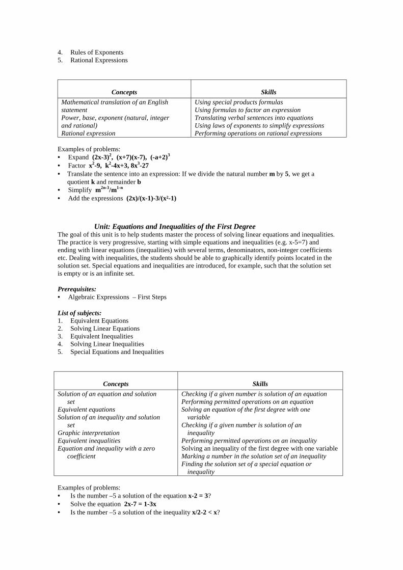
4. Rules of Exponents5. Rational Expressions

Concepts SkillsMathematical translation of an EnglishstatementPower, base, exponent (natural, integerand rational)Rational expression

Using special products formulasUsing formulas to factor an expressionTranslating verbal sentences into equationsUsing laws of exponents to simplify expressionsPerforming operations on rational expressions

Examples of problems:• Expand (2x-3)2, (x+7)(x-7), (-a+2)3

• Factor x2-9, k2-4x+3, 8x3-27• Translate the sentence into an expression: If we divide the natural number m by 5, we get a

quotient k and remainder b• Simplify m2n-3/m1-n

• Add the expressions (2x)/(x-1)-3/(x²-1)

Unit: Equations and Inequalities of the First DegreeThe goal of this unit is to help students master the process of solving linear equations and inequalities.The practice is very progressive, starting with simple equations and inequalities (e.g. x-5=7) andending with linear equations (inequalities) with several terms, denominators, non-integer coefficientsetc. Dealing with inequalities, the students should be able to graphically identify points located in thesolution set. Special equations and inequalities are introduced, for example, such that the solution setis empty or is an infinite set.

Prerequisites:• Algebraic Expressions – First Steps

List of subjects:1. Equivalent Equations2. Solving Linear Equations3. Equivalent Inequalities4. Solving Linear Inequalities5. Special Equations and Inequalities

Concepts SkillsSolution of an equation and solution

setEquivalent equationsSolution of an inequality and solution

setGraphic interpretationEquivalent inequalitiesEquation and inequality with a zero

coefficient

Checking if a given number is solution of an equationPerforming permitted operations on an equationSolving an equation of the first degree with one

variableChecking if a given number is solution of an

inequalityPerforming permitted operations on an inequalitySolving an inequality of the first degree with one variableMarking a number in the solution set of an inequalityFinding the solution set of a special equation or

inequality

Examples of problems:• Is the number –5 a solution of the equation x-2 = 3?• Solve the equation 2x-7 = 1-3x• Is the number –5 a solution of the inequality x/2-2 < x?

• Solve the inequality 1-3x/2 < x• Find the solution set of 2x-3 = 2x-4

Unit: Area and VolumeThe goal of this unit is to introduce the metric system, and enable students to acquire skills to workcomfortably with the metric system. The metric system is applied to units of length, area and volume, andstudents acquire the skills by solving problems related to geometrical shapes and volumes requiring theconversion of units.

Prerequisites:• Algebraic Expressions• Equations of the First Degree

List of subjects:1. The Metric System2. Calculating Area3. Calculating Volume

Concepts SkillsThe metric system, length, area and volum

unitsSub-unitsPrinciples in calculating areasPrinciples in calculating volumes

Multipling and dividing numbers by 10n

Converting length, area and volumes unitsCalculating area of a rectangle, square,

parallelogram, trapezoid, rhombus,circle, sector and ring

Calculating volume of a box, cube, prism,cylinder, pyramid, cone, sphere

Examples of problems:• Convert 1.2 m2 in cm2

• Find the price of 13 wood boards of the dimensions 60 cm x 25 cm x 4 cm if wood costs $125per m3

• Calculate in liters the volume of a ball whose diameter is 28 cm.

Algebra-2

Unit: Equations and Inequalities of the Second DegreeThe goal of this unit is to help students master the process of solving equations and inequalities of thesecond degree. Students advance progressively starting with simple quadratic equations (x²-9=0) andending with rather complicated equations including terms in the denominator, and irrational solutions.Solving a quadratic inequality uses the graphic method.

Prerequisites:• Algebraic Expressions• Equations of the first degree

List of subjects:1. Operations with Radicals2. Simple Quadratic Equations3. Solving Rational Quadratic Equations

4. Solving Irrational Quadratic Equations5. Solving Quadratic Inequalities

Concepts SkillsIrrational numberSolution and solution set of a quadratic

equationThe discriminant of an equation and the number of

solutionsSolution and solution set of a quadratic

inequalityThe quadratic function, sign of a function

Performing operations with irrationalnumbers

Solving a quadratic equation with rational orirrational solutions

Factoring a trinomialSolving a quadratic inequality by the graphic

method

Examples of problems:• Simplify √√√√3*√√√√5• Solve the equation x2-7x = 0• Solve the equation x2+3x = 4• Solve the equation 1-3/x = x• Find the solution set of 2x2+1 < 3x

Unit: Equations and Systems with Two VariablesThe goal of this unit is to help students master the process of solving a linear system of two linearequations with two variables. Special cases of parallel and coincide lines are also introduced.

Prerequisites: • Algebraic Expressions• Equations of the First Degree

List of subjects:1. Equations in Two Variables2. Solving Systems Graphically3. Solving Systems Algebraically4. Special Systems

Concepts SkillsEquation with two variablesSolution as an ordered pairThe graph of the solution setSystem of equations, solutionLinear combinationDependent and inconsistent systems

Checking if a given pair is solution of an equationBuilding solutions of an equationExpressing one of the variables in terms of the otherSolving a system graphicallySolving a system algebraicallyIdentifing proportional numbers and finding the

number of solutions of a systemDealing with a system with one parameter

Examples of problems:•••• Build solutions of the equation 2x-3y = 5• Solve graphically the system x+3y = -3 and 2x-5y = 4• Solve algebraically the system x+3y = -3 and 2x-5y = 4• For which value of m the system mx+3y = -3 and 2(m+1)x-5y = 4 has not a unique solution?

Unit: Quadratic Systems and Parameters

The goal of this unit is to help students master the process of solving quadratic systems, in which oneof the equations is linear and the other quadratic. They also solve an equation with a parameter and alinear system with a parameter. The unit explains the concept of a parameter of an equation. Studentsinvestigate the conditions that determine the number of solutions of an equation or a system.

Prerequisites: • Algebraic Expressions• Equations of the First Degree• Equations of the Second Degree• Systems in Two Variables

List of subjects:1. Quadratic Systems2. Linear Equations with a Parameter3. Linear Systems with a Parameter

Concepts Skills35Quadratic system, solutionGraphic meaning of the solutionsEquation with a parameter as a family

of equationsSystem with a parameter as a family of

systems

Solving a quadratic system by the substitutionmethod

Building a representative of a familyFinding a value of a parameter for certain conditionSolving an equation with a parameterSolving a system with a parameter

Examples of problems: • Solve the system 2x+y = -2 and 3x-2xy = 4 • Solve the equation 3(m+1)x –3 = x-3-m • Solve the system 2mx+y = -2 and mx-(m-1)y = 1

Unit: SequencesThis unit presents the concept of a sequence. It includes explicit and recursive sequences and theparticular cases of arithmetic and geometric sequences. Students investigate the relationship between theterms of a sequence using the formulas for the n-th. term, the sum, and they learn to find the differenceand the ratio. A special section is dedicated to exponential growth and decay in real life problems (such asgrowth of investment or population) as a special case of the geometric sequence. Simple exponentialequations are presented.

Prerequisites: • Algebraic Expressions• Equations of the First Degree• Equations of the Second degree• Systems in Two Variables

List of subjects:1. Explicit Definition2. Recursive Definition3. Arithmetic Progression4. Geometric Progression

Concepts SkillsSequence as a function from N to RTerms of a sequence as the values of the

Calculating terms in explicit sequenceFinding the rank of a given term

functionThe general termExplicit definitionRecursive definitionArithmetic progressionGeometric progressionExponential growth and decay

Using a recursive formula to findneighboring terms

Finding terms and sums in arithmetic andgeometric progression

Solving problems in exponential growth

Examples of problems:•••• Find two terms whose sum is -59 in the sequence defined by a(n) = 2-3n• Calculate the eighth term in the sequence defined by a(n) = 2a(n-1)-n if a(9) = 23• Calculate the sum of the terms a(11)+a(12)+…+a(23) in the arithmetic sequence defined by a(1)=-40 and d=7• A sum of $35,000 is invested at a rate of 4.6%. Calculate the value after 8 years

Word Problems and Probability

Unit: Problems on Percentages and NumbersThis unit presents word problems that can be solved directly by using formulas, or by solving a linearequations with one variable. Students are given percentage problems related to daily life. It alsopresents problems related to numbers where the relationship between the numbers has to be translatedinto a linear equation.

Prerequisites: • Algebraic Expressions• Equations of the First Degree

List of subjects:1. Problems on percentages2. Problems on numbers

Concepts SkillsPercentage, rate of increaseThe method of position, decimal representation of

an integer

Solving a real-life problemIdentifying steps in solving problems

Examples of problems:• In May the price of tomatoes was $50/ton. Six months later it was marked up by $15.81. Whatwas the percentage of increase in the price?• The sum of two numbers is 15. When one of them is divided by 2 the result is the other. Find thenumbers

Unit: Problems on Geometric Shapes and MotionThis unit strengthens the skills of translating a word problem into an equation and solving it. Theproblems presented in this unit are related to uniform motion and geometric shapes. Animation is used to

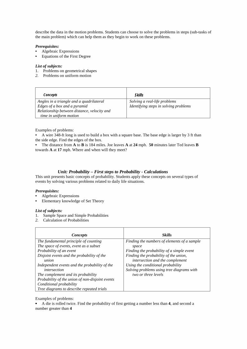
describe the data in the motion problems. Students can choose to solve the problems in steps (sub-tasks ofthe main problem) which can help them as they begin to work on these problems.

Prerequisites: • Algebraic Expressions• Equations of the First Degree

List of subjects:1. Problems on geometrical shapes2. Problems on uniform motion

Concepts SkillsAngles in a triangle and a quadrilateralEdges of a box and a pyramidRelationship between distance, velocity and

time in uniform motion

Solving a real-life problemsIdentifying steps in solving problems

Examples of problems:• A wire 348-ft long is used to build a box with a square base. The base edge is larger by 3 ft thanthe side edge. Find the edges of the box.• The distance from A to B is 184 miles. Joe leaves A at 24 mph. 50 minutes later Ted leaves Btowards A at 17 mph. Where and when will they meet?

Unit: Probability – First steps to Probability - CalculationsThis unit presents basic concepts of probability. Students apply these concepts on several types ofevents by solving various problems related to daily life situations.

Prerequisites: • Algebraic Expressions• Elementary knowledge of Set Theory

List of subjects:1. Sample Space and Simple Probabilities2. Calculation of Probabilities

Concepts SkillsThe fundamental principle of countingThe space of events, event as a subsetProbability of an eventDisjoint events and the probability of the

unionIndependent events and the probability of the

intersectionThe complement and its probabilityProbability of the union of non-disjoint eventsConditional probabilityTree diagrams to describe repeated trials

Finding the numbers of elements of a samplespace

Finding the probability of a simple eventFinding the probability of the union,

intersection and the complementUsing the conditional probabilitySolving problems using tree diagrams with

two or three levels

Examples of problems:•••• A die is rolled twice. Find the probability of first getting a number less than 4, and second anumber greater than 4

• Urn E contains 50 blue and 42 red balls. Urn F contains 69 blue and 13 red balls. An urn isselected and a ball is drawn. Find the probability that the ball is red.

Unit: Probability – Advanced topics to Probability - Combinatorics and DistributionsThis unit presents basic concepts of combinatorial and also presents advanced concepts of probabilitysuch as trials and the concepts of non-discrete probability, such as the normal distribution. Studentspractice these topics by solving problems related to daily life.

Prerequisites: • Probability – Calculations• Equations of the First Degree

List of subjects:1. Counting Problems2. Binomial Trials3. Normal Distribution

Concepts SkillsThe fundamental principle of countingSampling with/without replacementPermutationsCombinationsBernoulli trialBinomial distributionRandom variable, mean and standard deviationStandardized variable zThe normal curve of Gauss and the area under

the curveNormal distribution

Calculating samplings with/withoutreplacement

Calculating permutations andcombinations

Using Bernoulli formula to findprobabilities

Converting a random variable to astandardized variable

Calculating areas under the normal curveSolving problems in normal distributionUsing normal distribution to approximate

a binomial distribution

Examples of problems:• How many passwords containing 6 different letters can be formed using the letters{a,b,d,r,s,t,w,x}?• A fair coin is tossed 12 times. Find the probability to obtain “Heads” 8 or 9 times.• The main weight of newborns is 6.484 lb. and the standard deviation is 1.08 lb. Find theprobability that a newborn weighs less than 6.1 lb.

Coordinate Geometry and Trigonometry

Unit: Coordinate Geometry – Points, line, circle

The goal of this unit is to introduce the Cartesian coordinate system, points in the plane, distancebetween points and slope. Students learn about the graphic representation of a straight line as well asits representation as an equation. They also learn about the circle and its properties.

Prerequisites: • Algebraic Expressions• Equations of the first and second degree• Systems with two variables

List of subjects:1. Points in the Plane2. The straight line3. The circle

Concepts SkillsSystem of axes and coordinates of a

pointMidpoint and endpoints of a

segmentSlope of a lineDistance of two pointsSlope-intercept equation of a lineGeneral equation of a lineParallel and perpendicular linesIntersection point as solution of a

systemRadius and center of a circleTangent to a circle

Identifying a point by its coordinatesCalculating and estimating the slope of a lineFinding the midpoint and the endpoints of a segmentFinding the slope-intercept equation of a lineFinding the equation of a line passing through 2 points,

passing through a point and parallel orperpendicular to a given line

Checking if a point is inside, outside or on a circleFinding the equation of a circle given one of its

diametersFinding the equation of the tangent to a circleFinding the intersecting points of a circle and a lineFinding the equation of a circle passing through 3

given points

Examples of problems:• Find the endpoint B of a segment AB given A(3,-1) and the midpoint M(-2,-2).• Find the equation of the median AM of a triangle ABC given A(3,4), B(5,1) and C(-1,-3)• Find the equation of the circle whose diameter AB is A(5,2) and B(0,-3)

Unit: Coordinate Geometry - Ellipse, Hyperbola, ParabolaThe goal of this unit is to familiarize students with the ellipse, hyperbola and parabola. Their specialproperties are presented using animation, and students learn about their equations, foci and otherattributes.

Prerequisites:• Algebraic Expressions• Equations of the First and Second Degree• Coordinate Geometry – Points, Line, Circle

List of subjects:1. The ellipse2. The hyperbola3. The parabola

Concepts SkillsThe ellipse, the hyperbola and the parabola as

the focus of points having a certainproperty

Axes, foci, asymptotes, directrixThe tangent and the normal to the conic

sectionsProperties of the tangent and of the normal

Finding the foci and the semi-axes of anellipse

Finding the equation of an ellipseFinding the equation of the tangent

Examples of problems:• Find the equation of the tangent to the ellipse x2/20+y2/5 = 1 at point A(-4,1)• Find the set of points M in the plane verifying |MA-MB| = 16 given the points A(-5,0) and B(5,0)• Find the equations of the tangents to the parabola y = 6x2 passing through the point M(-3,4)

Unit: Trigonometry of the TriangleIn this unit students learn about the trigonometric functions defined in the right triangle, and about therelationship between those functions. They acquire skills needed to solve right and general trianglesusing the law of sines and law of cosines.

Prerequisites: • Algebraic Expressions• Equations of the First and Second Degree.

List of subjects:1. Functions Related to the Right Triangle2. Solving Triangles and Shapes

Concepts SkillsRight triangle and important geometrical

propertiesDefinition of SIN, COS, TAN in the right

triangleThe inverse functionsIdentity of 2 trigonometric expressionsFunctions of an obtuse angleLaws of cosinesLaw of sines

Expressing a trigonometric function in terms ofsides

Finding an angle using the inverse functionChanging a trigonometric expression using

identitiesSolving a right triangleSolving a right triangle using lettersSolving a general triangleCalculating a segment in a given figure

Examples of problems:• Find the angle x if SINx=0.88912• Find the radius R of the circumscribed circle of a triangle whose sides are a=5.22, b=4.1 and

c=6.87.

Unit: Advanced TrigonometryIn this unit the trigonometric functions that have been introduced in Trigonometry 1 are extended tothe domain R (the real line) using Pi and real numbers. Formulas for converting trigonometricfunctions of a sum to products, and a product to sum are presented. Students solve trigonometricequations using the relationship of the trigonometric functions and the formulas for converting sumsto products and vise versa.

Prerequisites: • Algebraic Expressions• Equations of the First and Second Degree

• Trigonometry in the Triangle

List of subjects:1. Definition of SINx, COSx, TANx2. Functions of the Sum of Two Angles3. Conversion of Sums into Products4. Solving Trigonometric Equations

Concepts SkillsThe unit circle as a real axis, the quadrantsThe condition that 2 numbers correspond to the same

pointDefinitions of SINx, COSx, TANxParity, sign and periodicity of the functionsSpecial valuesRadians and degrees, length of an arc, area of a

sectorFormulas for a sum, for the double angleWriting a sum as a productWriting of aSINx+bCOSx using one functionThe periodicity of the solutions of an equation in R

and in an interval

Identifying numbers on the unit circleChecking trigonometric equalities an

inequalitiesCalculating the value of a function

given another valueCalculating the length of an arc, area of

a sectorCalculating the exact value of SIN15°Using formula of a sum and the double

angle in identities and equationsFactoring a trigonometric expressionSolving trigonometric equations in R

and in an interval

Examples of problems:• Is the equality SIN(2x) = 2SINx ?

1. True for all values of x2. Always false3. True for some values and false for other values

• Express COS(8x) in terms of SIN(4x) only• Write the expression SIN(3x)+SIN(4x) as a product• Solve the equation 2COS(2x)+COSx = 1.2 in the interval [2,3]

Calculus and Linear Programming

Unit: Calculus - Derivative of PolynomialsThis unit presents basic concepts of calculus, such as the notion of the derivative, which isdemonstrated by animation and simple derivation laws. Students apply them to investigatepolynomials of the second, third and fourth degree.

Prerequisites: • Algebra• Coordinate Geometry – Points, Line

List of subjects:1. The notion of the derivative2. Investigating Polynomials

Concepts SkillsThe notion of the slope of a graph at a

pointDerivative of a function at a pointThe derivative function

Estimating and calculating of the derivative at apoint

Finding the derivative of a polynomial functionFinding the equation of the tangent to the graph at a

Increasing and decreasing functionStationary point and extremum point

pointFinding a point where the derivative has a certain valueInvestigating a polynomial function of the second,

third and fourth degree with algebraicapplications

Examples of problems:• Find the equation of the tangent to the graph of the function f(x) = x3-2x-1 at point (2,3)• Investigate the function f(x) = x3-2x-1 and find for which values of m the equation f(x) = m

has 3 solutions.

Unit: Calculus - Derivative of Elementary FunctionsThis unit presents advanced topic of derivatives; laws for derivation of real power, trigonometric,exponential and logarithmic functions are presented. Students investigate those functions.

Prerequisites: • Algebra• Trigonometry in the Triangle• Advanced Trigonometry• Calculus – Derivatives of Polynomials

List of subjects:1. Derivatives of Functions2. Investigating Functions

Concepts SkillsThe derivative of elementary functionsLaws of derivation

Calculating the derivative of an elementary function, ofa sum, a product, a quotient and a compositefunction

Investigating a rational, irrational, trigonometric,exponential, logarithmic and general powerfunction with algebraic applications

Examples of problems:•••• Calculate the derivative of f(x) = x2-3COS(2x-1)•••• Investigate the function f(x) = 2x-3/x in the domain R-{0} and find for which values of x thevalues of the function are positive

Unit: Calculus - IntegralsThis unit deals with the definite and the indefinite integral. Using the integral they calculate the areabounded between two graphs and the volume of a solid of revolution.

Prerequisites: • Algebra• Trigonometry in the Triangle• Advanced Trigonometry• Calculus – Derivatives of Elementary Functions

List of subjects:1. The Indefinite Integral2. Finding a Function by its Derivative

3. Calculating Area and Volume

Concepts SkillsAntiderivative, the indefinite integralRelationship between two antiderivativesThe graphic meaning of the constant of

integrationRules of integrationThe area functionSolid of revolution

Finding definite integral using the rules ofintegration

Finding a function knowing its derivative and apoint

Calculating the area between a graph and thex-axis

Calculating the area between two graphsCalculating the volume of a solid of revolution

Examples of problems:• Calculate the integral ∫∫∫∫SIN(2x)dx• Find the function f(x) given that f(1)=2 and f’(x) = 2x2-x-1•••• Calculate the area between the graphs of f(x) = -x2-x and g(x) = x2-1 between their

intersection points

Unit: Linear ProgrammingThis unit presents the concept of linear constrained problems, and the method to find the optimalsolution. Initially a system of linear inequalities is presented, and the feasible domain is searched.Methods to find the extreme values of a function defined on a polygonal domain are studied. Usingthis knowledge, students solve linear problems with two, three and four constraints.

Prerequisites: • Algebraic Expressions• Equations of the First Degree• System of two linear equations

List of subjects:1. Linear Inequalities with Two Variables2. Finding the Extreme Values of a Function3. Linear Programming Problems

Concepts SkillsLinear inequality with two variablesSolution set as a half-planeSystem of inequalities and the polygonal domainLinear function in 2 variables and its values on a

domainLevel lines and optimum of a linear functionConstraints of a problemThe feasible domain and the objective functionSolution of a problem in linear programming

Solving an inequality and a system ofinequalities

Building a system of inequalities givenits solution set

Calculating the values of a linearfunction in two variables

Using the vertices and level lines tofind the optimum

Solving a problem in linearprogramming with 2, 3 or 4constraints

Examples of problems:• Find the solution set of the inequality 2x-3y > 12• Find the maximum of the function f(x) = 2x+5y in the triangular domain defined by

A(12,20), B(25,30) and C(16,40).

• A Transportation Company has 18 big vans that can each carry 800 cube ft and 12 small vansthat can carry each 320 cube ft. The company has 20 drivers and has to carry luggage of10,000 cube ft. The use of a big van costs $250, a small costs $45 and each van can do onejourney. How many vans of each kind should the transportation company assign to keepminimum expenses.

Chapter 5: Teachers' ToolkitThe toolkit consists of three utilities, incorporated into one program. All three utilities are to be used byteachers.

5.1 Customization UtilityThe goal of this utility is to enable teachers to set the parameters controlling the behavior of the tutorialprogram for the students of MATH-TEACHER PLUS.There are few basic parameters that have been pre-determined by Math-Kal but they can be changed byteachers.

These parameters apply to each combination of Unit-Subject-Level. For each level there are four numbersthat control the flow of the program: • Minimum number of problems the student needs to solve before he or she can progress to the next

level. • Minimum grade the student needs to get in this level before he or she can progress to the next

level. • Activity mode of the calculator in the interactive tutorial (enabled/disabled) • Number of problems in this level of the test. • Duration, in minutes, assigned to each problem in this level of the test. • Activity mode of the calculator in the online test (enabled/disabled)

Note: The first two parameters determine whether the student can proceed to the next level.Students complete the practice in a certain level only after two conditions are met:1. The student solved a minimum number of problems2. The student achieved at least a minimal grade.Controlling these parameters allows the teacher to fine-tune the students' progress from one level to thenext, according to their ability, motivation, skills, etc.

Note: There are two parameters have an effect on the composition of the test and the allocated time.The on-line test is generated per subject. The parameters determine the number of the problems in the testand its duration. They allow teachers to define a customized test composing only of specific levels. Thiscan be done by assigning zero values to all the other levels. Teachers can increase or decrease theduration of the test based on the level of the students who take this test.There are pre-defined default values, set by Math-Kal, for all these parameters for each combination ofUnit-Subject-Level.

Note: you can customize the option of using the calculator.For each Unit-Subject-Level you can decide whether you allow the students to use the calculator.

Run the Customization Program if you wish: • To view the current settings • To change the current settings • To reset the values to default values.

When you run the program, you will be presented with a panel including all the units.Click the unit you wish to view or customize. This displays the unit panel. To customize values you canclick on the tutorial column or the test column.The default values appear on the panel primarily, however if you wish to change them, simply enter thenew values next to them.

If you just want to view the values, you can exit the program at this point. If you want to customize, enterthe new values and press the Customize button.The above panel shows how to customize the first subject in Algebraic Expressions - Intermediate.

The default values for completing the first level are 9 (the minimal number of problems to be solved) and80 (the minimal grade). The new values are 12 and 85. Clicking the Customize button make this changeeffective.

The figure below shows how to customize the test of this subject. The default values are 1 (number ofproblems in the first level), 1 in the second and 2 in the third. Now the new values are 2, 3 and 0. Thetime allocated to the problems has also been changed, so instead of 3 minutes, the customized test willlast 5 minutes per problem.

Note: You can customize any unit installed in your system.The process can be repeated for any unit that is installed in your system. Therefore, if Algebra-1 is theonly product installed in your system, you will be able to set values for all its four units, but not of theother products.

Note: You can choose for how long the customized values are effective.Once you click "Customize" you will be presented with a panel that allows you to specify how long thenew values are in effect. You can set them until midnight, or unlimited or until a specified date.

Note: You can reset all values of a unit to default.If you wish to reset all the values of a certain unit (for all its subjects) click the Default button.

Note: Who can run this program?During installation time, this program is installed in a lower folder than the folder where the tutorialprogram was installed. For example, if the product was installed in a network in the directory F:\Mathkal,then the Toolkit is located at F:\Mathkal\Ecustom directory. Only a user that has been granted read,write, create and erase rights to this directory can run this program.

5.2 Printed Tests GeneratorThis utility is a tool that enables you to print out lists of problems and answers on each unit and subject. Itallows you to build and print customized tests and homework for the students. You can compose a testfrom several units, subject s and levels. You can view the generated list and pick only the problems youreally want. You can produce as many lists that have the same level of difficulty, but include differentsets of problems. This is a tool that teachers find extremely helpful in their daily work.

To generate a test, go to the unit panel and click a button in the Test column. The list of the various levelswill be displayed. Next to each level button there is a white box in which you can type the number ofproblems of that kind.

Note: Type the number of problems you want to be printed out from this level in the white box.In the figure above for example, the user has specified 3 problems on “Volume of a right pyramid”, 2 on“Volume of a right cone”, 2 on “Volume of a sphere” and zero for all the other levels. The resulting list inthis case consists of 8 problems.

Note: Click the Test button to view the problems in the generated test.Clicking this button will present the test panel with all the generated problems. In this panel you candecide finally what problems will be included in the test. The Rearrange button allows you to get rid ofthe problems you are not interested in. You can also specify, for each problem, its point value by clickingthe Points button.Once you are satisfied with the composition of the test you can print it out. Click the Print button todisplay the print dialog where you can specify:

• The number of different lists to be printed out. • Whether you wish to get the printout of the answers.

• Whether you want to leave space between the problems so students can fill the answers on thesame sheet.

Note: You can build summarizing tests consisting of problems of various units/subjects/levels.The utility allows you to build a test consisting of variety of problems. You can repeat the process ofgenerating more problems and add them to the currently built test. Each time you choose another unit orsubject and specify the number of problems from each level, you are asked whether you want to build anew test or add the newly generated problems to the previously built test. You can add up to 12 problemsin each test. However, you can print as many lists as you wish, all have the same level of difficulty, but adifferent set of problems.

5.3 Student Management System (SMS)This part of the toolkit provides tools for administrating students' records. The management system usesdatabases, in which all data about the students' activities are recorded.The tool usually is used in two modes: • An initial mode has to be performed once per each class and can be carried out by a systemadministrator or teacher. In this mode, class IDs are assigned to each class and student IDs areassigned to students within the class. • A daily/weekly operating of the utility by teachers, to view students' records, printout reports andstatistics, and to backup the database files.

5.3.1 Initial mode - creating class ID and passwords

It is recommended that the system administrator will carry out this step. The initial task for each class isperformed in two steps: • Creating an empty database file • Adding names of students to the file

Use the Create button to build a new file. Each class will be assigned a unique three digit number ID.The created files will be saved by default to the folder …\SMS\Classlist\Common.

Optionally you can specify another folder instead of "Common", for example, Myfolder. In this case thefile will be saved to the folder …\SMS\Classlist\Myfolder.Providing the teacher name is optional but recommended. It will be in the various reports.The second step is adding names to the file. Click the Edit button to add names either manually or from atext file.Adding names to the class file automatically assigns a password to each student. The password is aunique identification. When students work with the tutorial program they have to provide a name, classID and a password. Essentially it is the password that identifies the students, and not their name, as namescan be written in a few different formats.

5.3.2 Working mode - producing reportsThe reports can be produced for a specific student or class.Select a class from the list of classes and then click the Report button to display a panel that enables youto produce reports for this class as a whole, or for the individual student in the class.In this panel you can specify what report you want to produce.

Student Report:To produce a student report check the Student Report radio-button, choose the student name from the listand click OK.This displays a panel in which you can view all the learning activities that the student has performed.You can specify what are the items (units, subjects) for which you want to see the report. You can alsospecify the starting and the closing dates.Click the Display Report button to see a detailed list on each activity.

Basically there are two lists, one for the interactive tutorial sessions and the other one for tests.Click the Print button to printout this report.

Class Report:Check the Class report radio button to get a list of all students in the class, their grades in a predefinedtime period, and their averages.Basically there are two lists, one for the interactive tutorial sessions and the other one for tests.Click the Print button to printout this report.

Class Statistics:Check the Class statistics radio button to get a list of all units and subjects that the students in this classworked on. You can select an item, a unit or a subject. Click Display Report to view charts of the meangrade and the standard deviation in the tutorial sessions and in the tests.Click the Print button to printout this report.

5.3.3 Backup and maintenance

Due to the importance of the data collected in the database files it is recommended that once in while the system administrator will backup the database.

Click the Backup button to display a backup panel. Then you can click the Copy button to save all the files in the database folder to a default folder, ..\Smsbkup.It is possible to change the default backup folder to any folder by clicking the Change folder button.In case the database files are lost or corrupted, copy manually all the files from the backup folder to..\SMS\Classlist\Common.Note: The folder \SMS\Classlist\Common must be present while students work in the tutorial program inorder to record their progress and bookmarks.

Regular maintenance may include moving students' records from a class or deleting from a class. Choosethe relevant class and click the Edit button on the tool bar. Click the View button to browse the names ofthe student in the selected class. Now you can either delete or move records.

Chapter 6: Technical Information

6.1 Hardware/Software Specifications

• IBM or compatible PC. • Windows 95/98, windows NT ,Windows 2000 • 586 or higher processor • 32MB memory • SVGA Graphic card with 16 bits color (High Color) or more

6.2 Screen ConfigurationIn order for the product to run properly, you need to make sure that the current configuration of yourscreen is set to a appropriate resolution and proper number of colors. The program can run with a screenresolution of 640x480 or higher, with small or large fonts.

For best results, it is recommended to run the program using resolution of 800x600 or higher.

You also have make sure that the number of colors is set to at least 16 bits, also called High Color.To set the resolution properly, use the Display Property in the control panel.

6.3 InstallationInsert the CD-ROM into the drive.Click setup.exe and follow the instructions.After the installation is completed, the group includes the following items:

• Readme • Tutorial program for students • Toolkit for teachers • Uninstall

The package can be installed in a network and in stand-alone stations.Network Installation: This installation should be performed by the network administrator. In addition, theadministrator needs to grant certain rights to appropriate folders.The name of the folder where MATH-TEACHER files are located depends on the version installed onyour system.To locate this folder, search for the folder D480GR. MATH-TEACHER files are located in the parentfolder of this folder.While working in network the administrator should grant students read right in this folder.In addition write right should be granted to the sub folder ..\SMS\CLASSLIST, and create right to the subfolder ..\GRSAVE

To run the Toolkit program, which consists of three utilities, grant rights to authorized users based on thefollowing information:

1. To operate the Printed Tests utility grant write right to the folder ECUSTOM2. To operate the Customization Utility grant write, create and erase rights to the folder ECUSTOM.3. To operate the Student Management System grant administrator right in the folder SMS.

In all cases the rights should be inherited to all sub folders.

6.4 TroubleshootingProblem: Unable to run the Toolkit Program from a network station.Reason: The user does not have the required rights to run the program.Action: The network administrator needs to grant the user read, write, erase and create rights in thesubfolder Ecustom.

Problem: Pictures are distorted.Reason: The screen configuration is not set properly; probably only 256 colors are effective.Action: Change the display properties to High Color.

Problem: The tutorial program is behaving strange for the students.Reason: The file, containing the parameters that determine the flow of the program, is corrupted.Action: Run the Toolkit Program, click Customization, get to the unit of interest and click the Defaultbutton.

6.5 Technical Support

If you need further technical support please send an Email to mathkal@netvision.net.il. If a problemoccurs while you are running the program, you can do the following:

1. Click the "Alt+PrtScrn" buttons. It will save the image of the panel in the clipboard.2. Click the E-mail button which exists on each panel. It will pop-up your email composer.3. Click "Ctrl+V" to paste the image into the email message.4. If needed, describe the problem in your own words.

Following the above steps enables you easily to send a message and describe a problem. This will greatlyhelp us to solve problems if they rise and provide you with the best customer support.