user's guide chartrunner lean

User's Guide

CHARTrunner Lean Version 1.0

Copyright © 2006-2011 Productivity-Quality Systems, Inc. Productivity-Quality Systems, Inc. is also known as PQ Systems, Inc.

All rights reserved. Printed in the United States of America. No part of this document may be reproduced, stored in a retrieval system, or transmitted, in any form by any means, electronic, mechanical, photocopying, recording, or otherwise, without the prior written permission of Productivity-Quality Systems, Inc.

The software contains proprietary information of Productivity-Quality Systems, Inc.; it is provided under a license agreement containing restrictions on use and disclosure and is also protected by copyright law. Reverse engineering of the software is prohibited.

Due to continued product development, this information may change without notice. The information and intellectual property contained herein is confidential between Productivity-Quality Systems, Inc. and the client and remains the exclusive property of Productivity-Quality Systems, Inc. If you find any problems in the documentation, please report them to us in writing. Productivity-Quality Systems, Inc. makes no warranties, express or implied, concerning the system, including all warranties of merchantability and fitness for a particular purpose.

CHARTrunner® is a trademark of Productivity-Quality Systems, Inc.

GAGEpack® is a trademark of Productivity-Quality Systems, Inc.

SQCpack® is a trademark of Productivity-Quality Systems, Inc.

PORTspy® is a trademark of Productivity-Quality Systems, Inc.

MEASUREspy® is a trademark of Productivity-Quality Systems, Inc.

DOEpack® is a trademark of Productivity-Quality Systems, Inc.

CQI-signals® is a trademark of Productivity-Quality Systems, Inc.

Total Quality Transformation® is a trademark of QIP, Inc. and Productivity-Quality Systems, Inc.

TQT® is a trademark of QIP Inc., and Productivity-Quality Systems, Inc.

Windows®, Windows® XP, Windows Server® 2003, Windows Vista®, Windows® 7, Windows Server® 2008 and Microsoft .NET™ framework are trademarks of the Microsoft Corporation.

All other brand and product names are trademarks or registered trademarks of their respective owners.

PQ Systems copyright notice

i

Contents

Welcome _________________________________________________________________________ 1

About CHARTrunner Lean ................................................................................................................ 2 About PQ Systems ............................................................................................................................ 3 How to contact PQ Systems .............................................................................................................. 4 Technical support .............................................................................................................................. 5 Maintenance support agreement....................................................................................................... 5 PQ Systems End-User License Agreement ...................................................................................... 6 Request for new features .................................................................................................................. 8 Types of CHARTrunner Lean Licenses ............................................................................................ 9

How to activate a per-computer (workstation) license ................................................................ 9 How to activate a concurrent-user license ................................................................................ 10

Introduction to CHARTrunner Lean __________________________________________________ 11

Terminology ..................................................................................................................................... 12 Finder tab .................................................................................................................................. 12 Chart view ................................................................................................................................. 13

How to customize the Finder tab ..................................................................................................... 13

Quick Start Guide ________________________________________________________________ 15

How to activate a per-computer (workstation) license .................................................................... 15 How to create a chart ...................................................................................................................... 16

How to select and filter subsets of data .................................................................................... 20 How to display a chart ..................................................................................................................... 21 How to edit a chart .......................................................................................................................... 22 How to save a chart as an image .................................................................................................... 22 How to move a chart to a different folder ........................................................................................ 23 How to share charts in a network folder .......................................................................................... 23 How to use a chart as a template .................................................................................................... 24 How to print a chart ......................................................................................................................... 24 How to copy a chart ......................................................................................................................... 24 How to delete a chart ...................................................................................................................... 25 Chart styles ...................................................................................................................................... 25

Appendix A: Chart title codes ______________________________________________________ 27

Appendix B: Formula references ____________________________________________________ 29

Attributes Control Charts (traditional) .............................................................................................. 29 chart .......................................................................................................................................... 29 p-chart ....................................................................................................................................... 30 c-chart ....................................................................................................................................... 32 u-chart ....................................................................................................................................... 33

Capability Analysis .......................................................................................................................... 34 Capability indices - two sided specifications ............................................................................. 34

ii Contents

Copyright © 2011

Capability indices - one-sided specification .............................................................................. 36 Performance indices - two-sided specifications ........................................................................ 37 Performance indices - one-sided specification ......................................................................... 39 Capability analysis - non-normal distributions .......................................................................... 40

Histogram statistics ......................................................................................................................... 48 Chi-squared test ........................................................................................................................ 48 Coefficient of variation .............................................................................................................. 51 Cpm........................................................................................................................................... 51 Cpu and Cpl .............................................................................................................................. 51 Data points, maximum and minimum ....................................................................................... 52 Dpm (DEFECTIVES per million) ............................................................................................... 52 Kurtosis ..................................................................................................................................... 52 Mean, range-bar and sigma-bar ............................................................................................... 53 Out-of-spec (actual) - statistics ................................................................................................. 53 Out-of-spec (theoretical) with z formulas .................................................................................. 54 Sigma lines ............................................................................................................................... 55 Sigma(e) and sigma(i)............................................................................................................... 55 Skewness .................................................................................................................................. 56 Specifications ............................................................................................................................ 56 Within # of sigma ...................................................................................................................... 56

Measurement control charts ............................................................................................................ 57 Measurement control charts (n=1) ............................................................................................ 57 Measurement control charts (n>1) ............................................................................................ 59

Tabular constants for computing variable control limits .................................................................. 65 Formulas for control charts limits .............................................................................................. 66

Appendix C: Treat as options _______________________________________________________ 67

Appendix D: Thoughts on using Order By ____________________________________________ 69

Potential problems ........................................................................................................................... 70

Index ___________________________________________________________________________ 73

1

In this chapter About CHARTrunner Lean ............................................................................... 2 About PQ Systems ........................................................................................... 3 How to contact PQ Systems ............................................................................ 4 Technical support ............................................................................................. 5 Maintenance support agreement ..................................................................... 5 PQ Systems End-User License Agreement ..................................................... 6 Request for new features ................................................................................. 8 Types of CHARTrunner Lean Licenses ........................................................... 9

CHAPTER 1

Welcome

2 CHARTrunner Lean User's Guide

Copyright © 2011

About CHARTrunner Lean CHARTrunner Lean is the next generation of charting software from PQ Systems. The software generates process performance charts from a variety of data sources to help you optimize your processes and demonstrate proof of quality performance. Designed with a focus on providing a simplified user-experience, CHARTrunner Lean streamlines the process of creating and customizing charts so that you can more easily make data-driven business decisions.

CHARTrunner Lean's features:

• Streamline the chart creation and editing process through an innovative user experience and workflow.

• Fetch data from various sources to provide process improvement information from enterprise data. • Use linking technology so that your SPC charts are always automatically up-to-date. • Include a chart creation wizard to guide you through the steps in the charting process. • Allow you to filter data from your database so you can focus your improvement. • Easily ask ad-hoc questions about your data through filtering to help focus your improvement efforts. • Provide a summary of all of your charts, so that you can focus your attention on processes that need

it most. • Let you select the specific SPC statistics to show on your charts. • Feature simplified chart annotation so that you can display descriptive information about your

process. • Allow multiple chart folders to be open concurrently to give you a broad view of your improvement

efforts. • Provide the ability to sort charts alphabetically, by date, by type, or by description. • Include thumbnail image chart browsing to help you navigate quickly to the chart you want to view. • Compute and displays multiple sets of control limits when your process shifts. • Provide direct on-chart support for control limits. • Option for multiple date formats on charts. • Give you complete control of how your control charts look, including colors, fonts, line styles, and fill

patterns with edits instantly appearing on your chart as you edit.

Welcome 3

Copyright © 2011

About PQ Systems For more than 25 years, PQ Systems, Inc. has been dedicated to helping organizations demonstrate proof of their quality performance. We are a full service quality management firm offering a comprehensive network of products and services designed to help all industries improve quality and comply with standards. PQ Systems provides the expertise, training, and software tools necessary to assist organizations through every step of the quality process. Our highly-regarded products have made us a leader in the industry, but our commitment to customer service and support keeps customers coming back.

Software

SQCpack® combines powerful statistical process control techniques such as variables, attributes, and Pareto charting with flexibility and ease of use.

GAGEpack® builds a complete database of an unlimited number of measurement devices, instruments, and gages from which users can generate a variety of reports. It supports ISO 9000, QS-9000, ISO/TS 16949-2009, ISO/IEC 17025, and other standards.

CHARTrunner® Lean is the next generation of SPC charting. The software generates statistical process control charts from a variety of data sources and performs SPC analysis to help demonstrate proof of quality performance.

CHARTrunner® draws SPC charts and performs statistical analysis using data that resides in other applications such as Microsoft Excel and Access.

DOEpack® is easy-to-use software that guides you through a logical, step-by-step process for planning, designing, implementing, and interpreting effective experimental designs.

Quality Workbench helps organizations keep day-to-day control over their quality systems in order to comply with ISO 9000 and other standards. It features document control, audits, nonconformities, customer care, and internet viewing modules.

Training and consulting

PQ Systems' consultants and trainers have extensive knowledge and experience in the areas of SPC, continuous improvement, ISO 9000, QS-9000, and trainer and leadership development in a wide variety of industries and organizations. In addition to customized in-house training, we offer public seminars.

Training tools

SPC Workout is an interactive multimedia training course on CD-ROM that provides effective step-by-step instruction on how to implement and apply SPC.

Gage Mentor is an interactive multimedia training course on CD-ROM that provides effective metrology training for operators, engineers, and quality personnel.

Total Quality Transformation® (TQT®) offers step-by-step help in facilitating quality improvement in organizations. Materials include "Practical Tools for Continuous Improvement", "Practical Tools for Healthcare Quality", "Foundations for Leaders", "Foundations of Quality", "Team Skills", "System Alignment Guide", "System Improvement Guide", and "Strategic Quality Planning Guide". TQT is part of the Transformation of American Industry training project, which has been used in a variety of manufacturing and service organizations since 1984.


Copyright © 2011

How to contact PQ Systems PQ Systems invites your questions and comments about our products and services.

Sales phone: 800-777-3020 or 937-813-4700

Sales email: [email protected]

PQ Systems, Inc.

210 B East Spring Valley Road

Dayton, OH 45458

Call sales for:

• General information to help you decide to purchase or evaluate the software

• To place an order or check the status of an order

You can send a fax to either Sales or Technical support at 937-813-4701. To ensure that your fax is delivered quickly to the right department, please send it to Attn: Sales or Attn: Technical support.

World Wide Web URL

http://www.pqsystems.com

International offices

http://[email protected]/�

http://www.pqsystems.com/�

Welcome 5

Copyright © 2011

Technical support Phone: 800-777-5060 or 937-813-4700

Email: [email protected]

Call PQ Systems’ experienced technical support team. Our experts can answer questions about software problems, data analysis, and applications.

Before you call, please follow these steps to help our technical advisors answer your questions quickly:

1. Have your license/serial number ready. It is listed in the About dialog box. You can access this dialog box by selecting Help > About from the menu.

2. Be at your computer, if possible.

3. Review the topic for which you have a question in the User's Guide and On-line Help.

Maintenance support agreement The product comes with an initial year of maintenance. After that, you must renew your product maintenance in order to ensure your continued access to the following great benefits:

1. Free software updates via download or CDROM - The product continues to evolve with suggestions from customers like you. Renewing your maintenance plan gives you access to 12 months of updates that include new features, improved usability, and compliance with the latest regulations from ISO 9000, JCAHO, FDA, and other regulatory bodies. http://www.pqsystems.com/support/SoftwareUpdates.php

2. Access to our legendary technical support - Our legendary support has kept customers coming back for more than 25 years. Renewing your maintenance plan will provide you access to our professional support staff. You have access to software and statistical application help via the phone, and in North America the number is toll-free.

3. Free subscription to Quality eLine - Quality eLine is our highly-acclaimed monthly electronic newsletter offering tips and techniques to enhance your software use and make your day-to-day work easier. Quality eLine includes Professor Cleary’s renowned and always entertaining Quality Quiz. Renewing product maintenance will ensure that you do not miss a monthly issue. http://www.pqsystems.com/eline/

4. Peace of mind - If your team depends on the product for its improvement charting, having a guaranteed direct line of contact to a committed support team offers priceless peace of mind, especially during an audit or survey. Renewing your maintenance support agreement ensures that the privileges of product maintenance continue uninterrupted.

Contact PQ Systems to renew your maintenance support agreement.


http://www.pqsystems.com/support/SoftwareUpdates.php�

http://www.pqsystems.com/eline/�


Copyright © 2011

PQ Systems End-User License Agreement This End-User License Agreement ("EULA") is a legal agreement between you (either an individual or a single entity) and PQ Systems, Inc. for the PQ Systems software that accompanies this EULA, which includes computer software and may include associated media, printed materials, "online" or electronic documentation, and Internet-based services ("Software"). An amendment or addendum to this EULA may accompany the software. YOU AGREE TO BE BOUND BY THE TERMS OF THIS EULA BY INSTALLING, COPYING, OR OTHERWISE USING THE SOFTWARE. IF YOU DO NOT AGREE, DO NOT INSTALL, COPY, OR USE THE SOFTWARE; YOU MAY RETURN IT TO YOUR PLACE OF PURCHASE FOR A FULL REFUND, IF APPLICABLE.

License

The Software may be licensed under the Per-Computer or the Concurrent-User license model.

Per-computer License Model - Under the per-computer license model, PQ Systems grants to you a nonexclusive right to install and use the Software on a single computer that is owned or controlled by you. You must purchase a registered per-computer license for each computer on which the Software is installed. If you use the Software through a network, you must still obtain individual licenses for the Software to cover each individual computer that will execute the Software through the network. For instance, if ten different computers will use the Software, each computer must have its own registered license, regardless of whether the Software is used at different times or concurrently.

Special provisions for using the per-computer license model in a terminal server environment - Windows Terminal Server, Windows Terminal Services, and various Citrix products are technologies that allow users from a variety of remote client devices to concurrently execute the Software that has been installed on a Windows server. All of these technologies are referred to as a terminal server environment under which the following licensing restrictions apply. A per-computer license must be purchased for each 'device' that 'runs' the Software. 'Device' encompasses client hardware devices, computers, workstations, terminals, or other digital electronic or analog devices that enable an end user to run the Software. To 'run,' or 'running,' the Software means using, accessing, displaying, running, or installing the Software, regardless of the medium of access to the product.

Concurrent-User License Model - The Concurrent-User License is offered under a subscription license term. Under the concurrent-user license model, PQ Systems grants to you a nonexclusive right to install the Software on multiple networked computers that are owned or controlled by you, and to concurrently use the Software, such that at any time, the total number of concurrent users of the Software is equal to or less than the number of concurrent users purchased by you. You agree to run a single instance of the PQ Systems' License Manager software within your network in order to limit usage of the Software such that no more than the purchased number of users can concurrently run the Software. You may install the PQ Systems' License Manager software on a backup computer to use only in the event that the primary computer fails. Any attempt to concurrently run more than one instance of the PQ Systems' License Manager software, or by any other means to concurrently run more than the purchased number of users, is in violation of this license and may result in termination of this license agreement.

License term

The term of this license may be perpetual or may be purchased in fixed units of time on a subscription basis.

Perpetual Term - A perpetual license term does not expire.

Subscription Term - A subscription license term expires at the end of the time period purchased by you. The Software will not function after the end of the purchased time period.

Welcome 7

Copyright © 2011

Evaluation period

Subject to the terms of this agreement, you are permitted to use the Software for evaluation purposes without charge during the evaluation period. If you want to use the Software after the evaluation period, then a license must be purchased. The evaluation period may vary from one PQ Systems product to another, but in no case does the evaluation period extend beyond 90 days from the first use of the Software.

Unregistered use of the Software after the evaluation period is in violation of U.S. and international copyright laws.

Product-specific provisions

CHARTrunner – This EULA does not apply when CHARTrunner software components are used by the server side of a client-server application. In that case, a different type of CHARTrunner license must be purchased. Contact PQ Systems for further information.

Further explanation of copyright-law provisions

You may not otherwise modify, alter, adapt, merge, decompile, or reverse-engineer the Software and you may not remove or obscure PQ Systems' copyright or trademark notices.

Per-computer License Model - You may transfer all of your rights to use the Software to another computer, provided that you transfer to that computer all of the Software, together with all copies, tangible or intangible, including copies in RAM or installed on a disk, as well as backup copies. Remember, once you transfer the Software, it may be used only on the single computer to which it is transferred. Except as stated in this paragraph, you may not otherwise transfer, rent, lease, sublicense, timeshare, or lend the Software. Your use of the Software is limited to acts that are essential steps in the use of the Software on your computer as described in the documentation.

Concurrent-User License Model - You may not transfer, rent, lease, sublicense, timeshare, or lend the Software. Your use of the Software is limited to acts that are essential steps in the use of the Software on your computer as described in the documentation. You may not use any means that permits more than the purchased number of users to concurrently use the Software.

Subscription Term - You may not use any means that permits the Software to run after the end of the purchased time period.

Electronic communications

The Software may from time to time transmit data to and from PQ Systems servers via the internet. This information transfer may be used to notify you when newer versions of the Software are available, for verifying license compliance, or for other purposes. PQ Systems will not collect any personally identifiable information from your computer during this process.

Governing law and general provisions


Copyright © 2011

This license statement shall be construed, interpreted, and governed by the laws of the State of Ohio, USA. If any provision of this statement is found void or unenforceable, it will not affect the validity of the balance of this statement, which shall remain valid and enforceable according to its terms. If any remedy provided is determined to have failed of its essential purpose, all limitations of liability and exclusions of damages set forth in the Limited Warranty shall remain in full force and effect. This statement may be modified only in writing signed by you and an authorized representative of PQ Systems, Inc. Use, duplication, or disclosure by the US Government of computer software and documentation in this package shall be subject to the restricted rights applicable to commercial computer software (under DFARS 52.227-7013). All rights not specifically granted in this statement are reserved by PQ Systems, Inc.

Disclaimer of warranty

THIS SOFTWARE AND THE ACCOMPANYING FILES ARE SOLD “AS IS” AND WITHOUT WARRANTIES AS TO PERFORMANCE OR MERCHANTABILITY OR ANY OTHER WARRANTIES WHETHER EXPRESSED OR IMPLIED. Because of the various hardware and software environments into which the Software may be put, NO WARRANTY OF FITNESS FOR A PARTICULAR PURPOSE IS OFFERED.

Good data processing procedure dictates that any program be thoroughly tested with non-critical data before relying on it. The user must assume the entire risk of using the Software. ANY LIABILITY OF THE SELLER WILL BE LIMITED EXCLUSIVELY TO PRODUCT REPLACEMENT OR REFUND OF PURCHASE PRICE.

PQ SYSTEMS, INC.

Corporate Headquarters: 210 B East Spring Valley Road, Dayton, Ohio 45458, USA, (937) 813-4700, http://www.pqsystems.com. International Offices: Australia 03-9770-1960, The United Kingdom 0044 (0) 1704 871465.

All PQ Systems products are trademarks of Productivity-Quality Systems, Inc., Copyright (c) 1998-2011 Productivity-Quality Systems, Inc.

All rights reserved.

Request for new features PQ Systems wants to provide you with software that meets your quality needs. To do this, we need your input. If there is a feature, function, or operation that you would like to see in a future version of the software, please contact Technical support by email at [email protected] or by phone at 800-777-5060 or 937-813-4700.

http://www.pqsystems.com/�


Welcome 9

Copyright © 2011

Types of CHARTrunner Lean Licenses CHARTrunner Lean can licensed in a variety of options.

Enterprise solutions: CHARTrunner Lean enterprise solutions expand your SPC charting options across multiple plants, across the globe, and in the cloud. If you need SPC charts and analysis for your global enterprise, we offer the following solutions.

CHARTrunner Lean concurrent-user license: Concurrent-user licenses, also called floating licenses or flexible-use licenses, allow customers to install CHARTrunner Lean on terminal servers, Citrix servers, or an unlimited number of computers. A license server meters usage of CHARTrunner Lean, enabling no more than the licensed number of users to simultaneously run the software. The concurrent-user license model offers the following advantages to enterprise customers:

• You install CHARTrunner Lean on a terminal server or a Citrix server only once, rather than having to install it on many computers throughout your organization.

• The administration of license management is simple, since there is only one license number to purchase and renew.

• A concurrent-user license is economical, since it allows sharing of floating licenses among multiple users. This provides you with enterprise-wide software access at a reasonable cost.

SQL Server Integration: CHARTrunner Lean links to data stored in SQL Server seamlessly so that you can begin to gain value from your SQL data instantly.

• SPC charts refresh as new data is added to the database, so charting is real time.

• CHARTrunner Lean charts data from SQL Server tables or views so that previously imprisoned data is set free for charting and critical decision-making.

• Entering quality metrics into SQL Server is made easy with PQ Systems solutions. Contact us to learn more.

Data in the cloud: CHARTrunner Lean is SQL Azure ready for charting data in the cloud. Whether you have plants in multiple states or multiple countries, CHARTrunner Lean can create SPC charts from your SQL Azure data in the cloud, regardless of where it is being generated.

CHARTrunner-m: CHARTrunner-m is control chart monitoring software that alerts you when a process is statistically out of control or outside a specified range. CHARTrunner-m keeps watch over your processes and notifies you when a condition occurs that needs attention. Whether you have tens of SPC metrics locally or hundreds of SPC metrics globally that demand your attention, CHARTrunner-m can automate your process monitoring.

How to activate a per-computer (workstation) license Before you begin this procedure, you will need your License Number and Update Code in the CHARTrunner Lean License Registration certificate or email.

To activate a per-computer (workstation) license:

1. Click Activate License in the License group.


Copyright © 2011

• The PQ Systems License Utility dialog box displays.

2. In the License Number field, enter your license number

3. In the Update Code field, enter your update code.

4. Click Update.

How to activate a concurrent-user license Summarized instructions for activating a concurrent-user license can be found at http://www.pqsystems.com/concurrent/ConcurrentUserLicensingQuickStartGuide.pdf.

Detailed instructions for activating a concurrent-user license can be found at http://www.pqsystems.com/support/PQLM8.0_AdminGuide.htm.

http://www.pqsystems.com/concurrent/ConcurrentUserLicensingQuickStartGuide.pdf�

http://www.pqsystems.com/support/PQLM8.0_AdminGuide.htm�

11

CHARTrunner Lean's interface is designed with a focus on providing a simplified user-experience to streamline the process of creating and customizing charts.

In this chapter Terminology ................................................................................................... 12 How to customize the Finder tab ................................................................... 13

CHAPTER 2

Introduction to CHARTrunner Lean


Copyright © 2011

Terminology

Finder tab When you open a CHARTrunner Lean you will notice a new look. Menus and toolbars have been replaced by the Ribbon, which contains tabs that you click to get to commands.

1. The Ribbon is a panel that displays command buttons and icons. The two parts of the Ribbon are:

• Groups - Groups are sets of related commands. They remain on display and readily available, giving you visual aids.

• Commands - Commands are arranged in groups. A command can be a button, a menu, or a box where you enter information.

2. The Finder displays the Chart Locations list and the associated charts.

3. The Chart Locations list displays the available charts.

4. The Chart Location Remove button removes a chart location from the Chart Locations list.

5. The Chart Location Add button adds a chart location to the Chart Locations list.

6. The Arrange By drop-down allows you to select the Finder Arrange Options for the Finder tab.

7. The View drop-down allows you to select the Finder View Options for the Finder tab.

Introduction to CHARTrunner Lean 13

Copyright © 2011

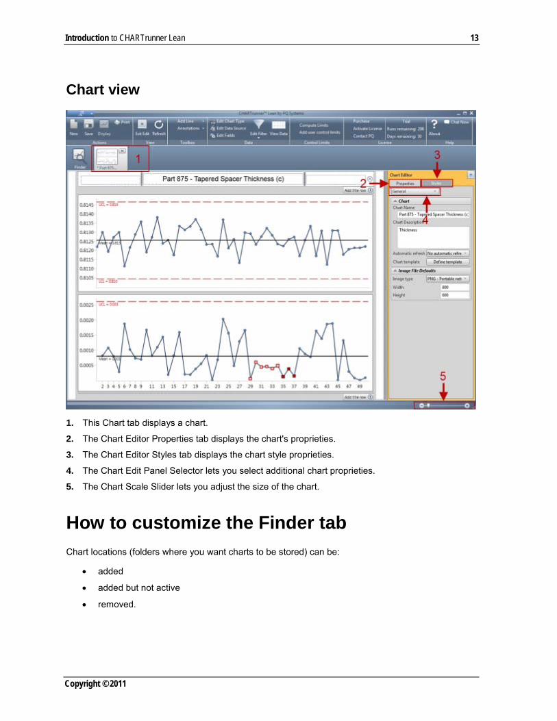
Chart view

1. This Chart tab displays a chart.

2. The Chart Editor Properties tab displays the chart's proprieties.

3. The Chart Editor Styles tab displays the chart style proprieties.

4. The Chart Edit Panel Selector lets you select additional chart proprieties.

5. The Chart Scale Slider lets you adjust the size of the chart.

How to customize the Finder tab Chart locations (folders where you want charts to be stored) can be:

• added

• added but not active

• removed.


Copyright © 2011

Click Add to browse for folders and add them to the list of chart locations. To keep the chart location, but not display the contents of this chart, uncheck the location. Click Remove to the right of a chart location name to remove the chart location from the list of chart locations.

Charts in the Finder can be viewed as:

• large icons

• medium icons

• small icons

• in a list of chart names

• as a detailed list.

The icons are thumbnail images of your chart. Select the Finder View Options in the upper right corner of the Finder.

Charts in the Finder can be arranged and sorted (ascending or descending) by

• chart name

• chart type

• description of the chart

• date the chart was modified

• by which charts have been selected.

Select the Finder Arrange Options in the upper right corner of the Finder.

15

In this chapter How to activate a per-computer (workstation) license ................................... 15 How to create a chart ..................................................................................... 16 How to display a chart .................................................................................... 21 How to edit a chart ......................................................................................... 22 How to save a chart as an image .................................................................. 22 How to move a chart to a different folder ....................................................... 23 How to share charts in a network folder ........................................................ 23 How to use a chart as a template .................................................................. 24 How to print a chart ........................................................................................ 24 How to copy a chart ....................................................................................... 24 How to delete a chart ..................................................................................... 25 Chart styles .................................................................................................... 25

How to activate a per-computer (workstation) license Before you begin this procedure, you will need your License Number and Update Code in the CHARTrunner Lean License Registration certificate or email.

To activate a per-computer (workstation) license:

1. Click Activate License in the License group.

CHAPTER 3

Quick Start Guide


Copyright © 2011

• The PQ Systems License Utility dialog box displays.

2. In the License Number field, enter your license number

3. In the Update Code field, enter your update code.

4. Click Update.

How to create a chart Charts are divided into six categories:

1. Measurement control charts for individual values

2. Measurement control charts for subgroup (average) values

3. Distribution and Capability analysis charts

4. Count or Classification (attributes) control charts

5. Pareto charts

6. Line charts.

To create a chart:

1. Click New in the Actions group.

Quick Start Guide 17

Copyright © 2011

• The Edit Chart Type dialog box displays.

• Hover the mouse pointer on a chart thumbnail to display a description that will help you select the

appropriate chart type.

2. Click the chart type you want to create.

3. Click Next.


Copyright © 2011

• The Edit Data Source dialog box displays.

4. In the Data Source field, select the data source.

• The options include: Access, Excel, or SQL Server.

5. In the Data file (or Server) field, select the path and name of the data file or server.

6. In the Worksheet, Table/Query, or Connection field, select the name of the worksheet, file, table, or query.

7. Click Next.


Copyright © 2011

• The Edit Fields dialog box displays.

8. Select the columns in the data to use.

9. Select how the chart will use each column.

• Appendix C: Treat As Options lists the options available based on the chart type.

• Until the requirements of the chart type are met, red text indicates the remaining tasks that need to be completed. Clicking View Data can help you complete this step. When you click View Data, all columns of data in the Worksheet/Table or only the columns you have selected display.

• Once the requirements of the chart type are met, you can select a subset of the data using the Filtering features and/or the Use Last n rows of your data option.

Note: PQ Systems recommends using an Order By column to indicate the order of the data, such as a Date/Time column. By indicating an Order By column, control limits will be displayed and extended in the manner you expect. In addition, any annotations with specific points on the chart move with the data.


Copyright © 2011

How to select and filter subsets of data New charts are created by pointing to data in a spreadsheet or database table. By default, charts use all of the data. You can use the Filtering features to select a subset of the data. For example, you may want to select only data from January or only data for a specific department.

To display the Edit Filter dialog box, click Edit Filter in the Data group or click Edit Fields in the Data group and then click Edit the Filter.

Click Add condition, Add date range, and/or Add clause to add a condition to the filter. Click Remove this Filter condition ( ) to remove a condition from the filter.

When you add a condition, you must select a column from the data source. When you click Add condition, the options include all the column names. When you click Add date range, the options include the date/time columns from the data source.

Click Add condition when you want to filter things like:

• Operator is equal to Mary

• Shift is equal to 1

• Quantity is greater than 1000

• Supplier is not equal to Wintronics

• Date is greater than 01/01/2012.

Click Add date range when you want to filter things like:

• MfgDate is within Last Month

• MfgDate is within Last 7 days

• ShipDate is within Last 2 quarters.


Copyright © 2011

Click Add clause when you want to add a complex expression not handled by the other buttons. For example:

• (Operator = Sam or Operator = Mary) AND Date > 01/01/2012

When using Add clause, you must use symbol operators. For example:

Correct Incorrect Operator = Sam Operator is equal to Sam

Following is a list of available operators.

Operator Definition = is equal to

<> is not equal to

> is greater than

< is less than

>= is greater than or equal to

<= is less than or equal to

LIKE pattern matching i.e., LIKE *.dat

You can combine conditions, date ranges, and clauses to define a subset of data to include in a chart. Be careful not to define a filter that does not return any records because no record will meet all the conditions. For example:

• Operator = Sam AND Operator <> Sam

The bottom of the Edit Filter dialog box contains commands that allow you to specify the filter's settings. To see how a condition will select data, click View. The where clause that is created displays. If the filter has recently been added or modified, click Click to update "Rows returned' to refresh the filter results.

To see the data your filter selects, click View Data.

How to display a chart To display a single chart:

1. From the Finder, click a chart.

2. Click Display in the Actions group or right-click on the chart and select Display or Display full screen.

• If you select Display, you can also edit the chart.

• If you select Display full screen, the chart displays in Slide Show mode. Pressing Page Down or the right arrow key advances to the next chart.

To display multiple charts, each in its own Chart tab:

1. From the Finder, select multiple charts.

• To select multiple charts in Icon view, select the chart in the top left corner.


Copyright © 2011

• To select multiple charts in Details or List view, select the box next to the chart, or select multiple charts by pressing CTRL or SHIFT and clicking the chart names.

2. Click Display in the Actions group or Display Slideshow in the Presentation group.

• You can also right-click on any of the charts and select Display full screen.

• Pressing Page Down or the right arrow key advances to the next chart.

How to edit a chart To edit a single chart:

1. From the Finder, click a chart.

2. Click Edit Chart in the View group or right-click on a chart and select Edit.

• The chart displays in the Chart Editor.

• To edit a chart while displaying it, click Edit Chart in the View group.

3. Make any necessary edits to the chart.

4. Click Save in the Actions group.

• The chart is saved to the selected chart location.

Refer to Editing Charts for detailed instructions on editing charts.

How to save a chart as an image To save a chart as an image:

1. In the Finder, right-click on a chart and select Save as image.

• The Save as image dialog box displays.

2. Select an image type.

3. Select the image size.

4. Click Browse.

• The Browse For Folder dialog box displays.

5. Select an output location for the image.

6. Click Save.

7. Click OK.

• The chart image is created and saved in the specified location.

To save a chart as an image when the chart is displayed:

1. Click the CHARTrunner drop down arrow and select Save as > Image.

2. Select an image type.

3. Select the image size.

4. Click Browse.


Copyright © 2011


5. Select an output location for the image.

6. Click Save.

7. Click OK.

• The chart image is created and saved in the specified location.

How to move a chart to a different folder To move a chart to a different folder:

1. In the Finder, right-click on a chart.

2. Select Move to active chart location.

• The Choose Destination dialog box displays.

3. Select a destination.

4. Click OK.

• The chart is moved to the selected destination.

How to share charts in a network folder Saving a chart on the network is an easy way to share your charts with others. All you have to do is save the chart and data in a folder on the network. Anyone who has access to that folder just needs to add the folder to their Chart Locations list.

To add a folder to Chart Locations:

1. Click Add in the Chart Locations list.


2. Select the folder.

3. Click OK.

• The folder is added to the Chart Locations list.


Copyright © 2011

How to use a chart as a template If you have created and perfected a chart that fits your exact needs, you can use that chart as a template for all other charts created in that particular chart category.

To use a chart as a template:

1. From the Finder, click on a chart.

2. Click Display in the Actions group.

3. Click Edit Chart in the View group.

• The Chart Editor displays.

4. Click Define template.

• A CHARTrunner Lean warning dialog box displays.

5. Click Yes to use the template for all other charts in the same category.

• The chart is now the default for all new charts created in the category.

How to print a chart To print a chart:

1. Click Print in the Actions group or right-click the chart and select Print.

• The Print dialog box displays.

2. Click OK to print the chart.

How to copy a chart If you have a lot of charts to create, you can start with one chart that has been edited to meet your needs, copy the chart and change only what is different. For example, if you want a chart for each of three production shifts, you can create a chart for one production shift and then copy and edit the chart for the second and third production shifts.

To copy a chart:

1. From the Finder, right-click a chart and select Copy.

• The copied chart displays in the Finder.

2. Click Edit Chart in the View group.

• The copied chart displays in the Chart Editor.

3. On the Proprieties tab, in the Chart Name field, enter the name of the chart.

4. Click Save in the Actions group.

• The chart is saved.


Copyright © 2011

How to delete a chart To delete a chart:

1. In the Finder, click a chart.

2. Press Delete to delete the chart.

Chart styles Each chart contains unique styles or chart aesthetics. Once you select a chart style, you can make it the default style for all new charts by clicking Define template in the Chart Editor on the Properties tab in the Chart heading panel.

PQ Systems recommends that you select color preferences that provide maximum clarity and contrast. If you plan on displaying the chart with a projector, keep in mind that some color schemes do not project well.

Refer to Editing Charts for detailed information on chart styles.

27

You may insert various title codes into all chart titles. These codes allow the software to substitute an appropriate value whenever the chart is rendered. The simplest example is the @D title code. If you place this in a chart title, today's date will replace the @D, when the chart is generated. So a chart title that is entered like this:

Chart generated on @D

Will be displayed on the chart as:

Chart generated on 07/05/2007

Title codes can be used to save time while defining charts. For example, if you want the chart name to appear as a chart title, you could manually type in the chart name as a title. However, if you make a copy of the chart or change the name of the chart, the chart title will have to be manually edited. If you use the @CTN title code – then the chart can be copied and renamed and will always display the appropriate chart name.

The @IMAGE(FilePath,PctWidth) title code displays the image file specified by ‘FilePath’. The desired width of the displayed image is specified as a percentage of the chart width by ‘PctWidth’. The aspect ratio of the image will be maintained as it is resized in order to fit within the specified width of the chart. If the image file specified by ‘FilePath’ cannot be found using the specified path, then CHARTrunner will try to find the image file in the current chart folder, and if that fails, it looks in the SysData folder. The following image file types are supported: BMP, JPG, JPEG, PNG, WMF and EMF. In general the best results are obtained with WMF or EMF since this type of image file can be resized without loss of quality, although it can be challenging to properly create WMF or EMF image files.

List of chart title codes

@CTD Chart description

@CTF Filename for chart

@CTN Chart name

@D, @DATE Current date

@DT, @DATETIME Current date and time

@IMAGE(FilePath,PctWidth) Display image file

@LSL Lower specification value

@SGF, @FILTER Current filter – only if it is enabled

@T, @TIME Current time

@TSL, @TS Target (or Nominal) value

@USL Upper specification value

CHAPTER 4

Appendix A: Chart title codes


Copyright © 2011

NOTE: Not all statistical title substitutions will have meaning for all chart types. For example, let's say that you put @CPK in a title of a Pareto chart. Since there is no context for calculating Cpk in a Pareto chart, the @CPK will be rendered in the title as nothing (i.e., zero length text), rather than as the computed Cpk statistic. This holds true for all title codes that are inappropriate for the current chart context.

29

In this chapter Attributes Control Charts (traditional) ............................................................ 29 Capability Analysis ......................................................................................... 34 Histogram statistics ........................................................................................ 48 Measurement control charts .......................................................................... 57 Tabular constants for computing variable control limits ................................. 65

Attributes Control Charts (traditional)

chart Nonconforming with Constant Sample Size

n = Sample size

k = number of samples

npi = the number of nonconforming units in the ith sample

CHAPTER 5

Appendix B: Formula references


Copyright © 2011

Mean

Standard deviation (sigma)

np-chart, upper control limit

np-chart, center line

np-chart, lower control limit

p-chart Nonconforming with Varying Sample Size

n = Sample size


ni*pi = the number of nonconforming units in the ith sample

Appendix B: Formula references 31

Copyright © 2011

Mean


p-chart, upper control limit

p-chart, center line

p-chart, lower control limit


Copyright © 2011

c-chart Nonconformities with Constant Sample Size

Sample size is constant:


ci = the number of nonconformities in the ith sample

Mean


c-chart, upper control limit

c-chart, center line

c-chart, lower control limit


Copyright © 2011

u-chart Nonconformities with Varying Sample Size

ni = number of units in ith sample


ci = the number of nonconformities in the ith sample

Mean


u-chart, upper control limit

u-chart, center line

u-chart, lower control limit


Copyright © 2011

Capability Analysis

Capability indices - two sided specifications Process capability refers to what a process is "capable" of doing. Process performance refers to what a process is "actually" doing. Process capability compares the specification spread to the inherent variation of a process (6 sigma based on estimated sigma). The standard analysis assumes:

1. The process is statistically stable (in-control)

2. The process output is normally distributed with:

Measures of Capability are: Cp, Cpk, and Cr which use estimated sigma in the calculations.

Cp

The Cp index is used to summarize a system's ability to meet two-sided specification limits (upper and lower). It uses estimated sigma and, therefore, shows the systems potential to meet the specifications. However, it ignores the process average and only considers the spread of the specification compared to the process spread. If the process is not centered in the specifications, Cp by itself may be misleading.

Interpreting Cp

Cp > 1 The specification spread is larger than the process spread (good)

Cp = 1 The specification spread equals the process spread (on the edge)

Cp < 1 The specification spread is smaller than the process spread (not good)

The higher the Cp value the smaller the spread of the process output in comparison to the spread of the specification. Cp is a measure of spread only. If the process is well centered, Cp will serve as a relatively good measure of process performance. However, a process with a narrow spread (a high Cp) may not meet customer needs if it is not centered within the specifications. Cpk takes into account where the process is centered. If both Cp and Cpk are used together, the spread and the centering can be evaluated at the same time.


Copyright © 2011

Cpk

Cpk is a capability index which indicates how well a process is doing in terms of meeting specification limits. Cpk calculations use estimated sigma. Since Cpk takes the location of the process average into account, the process does not need to be centered on the target value for this index to be useful. However, since Cpk is calculated using the specification limit closest to the mean, it penalizes the process by assuming that both distances to the specification limits from the mean are equal to the smallest one. This does produce a desired result which is to get suppliers to center their processes in order to maximize Cpk. In fact, if the process is centered in the specification (on nominal), Cp and Cpk will be equal.

Interpreting Cpk

Cpk > 1 The process is expected to produce more than 99.7% good

Cpk = 1 The process is expected to produce at least 99.7% good

Cpk < 1 The process is not expected to produce at least 99.7% good

Cpk should be used in conjunction with the Cp index. Cpk indicates what the process is doing and Cp indicates what it could do if it was centered. If they are not equal, some decision rules can be instituted indicating what action should be taken.

Cp > 1 and Cpk < 1 Center the process making Cpk >1

Cp < 1 and Cpk < 1 Need to improve the process by narrowing the process spread.

Cp >= 1 and Cpk >= 1 Celebrate and change reference value to 1.33, 1.67, or 2.00.

Where:


Copyright © 2011

Cr

The Cr capability ratio is used to summarize how much of the specification spread is being used by the process spread. It is the inverse of Cp and like Cp, Cr does not consider process centering. The formula is:

When the Cr value is multiplied by 100, the result shows the percent of the specifications that are being used by the variation in the process.

Capability indices - one-sided specification There are many specifications that are expressed as one-sided. For example, many strength tests have a minimum but no maximum value. In other cases, the value is often bound by zero (flatness, roundness, etc.) and yet, zero is often the value one would like to achieve. Since Cpk and Ppk are based on the specification closest to the mean, both indices would be reduced as the objective is achieved. Consequently, the use of only one specification solves this dilemma. For completeness, the calculations for Cp = Cpk and Pp= Ppk.

For one-sided specifications, calculations for Cp, Cr, and Cpk are:

For upper specification For lower specification

NOTE: When using one-sided specifications, Cp and Cpk are the same.


Copyright © 2011

Performance indices - two-sided specifications Performance capability refers to what a process is "capable" of doing. Process performance refers to what a process is "actually" doing. Performance capability compares the specification spread to the inherent variation of a process (6 sigma based on sigma of the individual values). The standard analysis assumes:

1. The process is statistically stable (in-control)

2. The process output is normally distributed with:

Measures of Performance are: Pp, Ppk, and Pr which use sigma of the individual values in the calculations.

Pp

The Pp index is used to summarize a system's ability to meet two-sided specification limits (upper and lower). It uses sigma of the individual values and, therefore, shows the systems potential to meet the specifications. However, it ignores the process average and only considers the spread of the specification compared to the process spread. If the process is not centered in the specifications, Pp by itself may be misleading.

Interpreting Pp

Pp > 1 The specification spread is larger than the process spread (good)

Pp = 1 The specification spread equals the process spread (on the edge)

Pp < 1 The specification spread is smaller than the process spread (not good)

The higher the Pp value the smaller the spread of the process output in comparison to the spread of the specification. Pp is a measure of spread only. If the process is well centered, Pp will serve as a relatively good measure of process performance. However, a process with a narrow spread (a high Pp) may not meet customer needs if it is not centered within the specifications. Ppk takes into account where the process is centered. If both Pp and Ppk are used together, the spread and the centering can be evaluated at the same time.


Copyright © 2011

Ppk

Ppk is a capability index which indicates how well a process is doing in terms of meeting specification limits. Ppk calculations use sigma of the individual values. Since Ppk takes the location of the process average into account, the process does not need to be centered on the target value for this index to be useful. However, since Ppk is calculated using the specification limit closest to the mean, it penalizes the process by assuming that both distances to the specification limits from the mean are equal to the smallest one. This does produce a desired result which is to get suppliers to center their processes in order to maximize Ppk. In fact, if the process is centered in the specification (on nominal), Pp and Ppk will be equal.

Interpreting Ppk

Ppk > 1 The process is expected to produce more than 99.7% good product

Ppk = 1 The process is expected to produce at least 99.7% good product

Ppk < 1 The process is not expected to produce 99.7% good product

Ppk should be used in conjunction with the Pp index. Ppk indicates what the process is doing and Pp indicates what it could do if it was centered. If they are not equal, some decision rules can be instituted indicating what action should be taken.

Pp > 1 and Ppk < 1 Center the process making Ppk greater than one

Pp < 1 and Ppk < 1 Need to improve the process by narrowing the process spread.

Pp >= 1 and Ppk >= 1 Celebrate and change reference value for Ppk to 1.33, 1.67, or 2.00.

Where:


Copyright © 2011

Pr

The Pr capability ratio is used to summarize how much of the specification spread is being used by the process spread. It is the inverse of Pp and like Pp, Pr does not does not consider process centering. The formula is :

When the Pr value is multiplied by 100, the result shows the percent of the specifications that are being used by the variation in the process.

Performance indices - one-sided specification There are many specifications that are expressed as one-sided. For example, many strength tests have a minimum but no maximum value. In other cases, the value is often bound by zero (flatness, roundness, etc.) and yet, zero is often the value one would like to achieve. Since Ppk and Cpk are based on the specification closest to the mean, both indices would be reduced as the objective is achieved. Consequently, the use of only one specification solves this dilemma. For completeness the calculations for Pp = Ppk and Cp = Cpk.

For one-sided specifications, calculations for Pp, Pr, and Ppk are:


NOTE: When using one-sided specifications, Pp and Ppk are the same.


Copyright © 2011

Capability analysis - non-normal distributions PQ software uses Pearson curve-fitting techniques to analyze non-normal distributions. These techniques give useful measures of process capability in some situations, when using the standard process capability study would be misleading and inappropriate.

Pearson curve techniques apply to a wide range of distributions. But before applying the techniques to your own data, it is important to understand a few points:

1. These techniques are meant to be used for understanding process variability in situations where the parameter is expected NOT to vary according to a normal distribution. That is, some parameters will not vary normally because of the nature of the measured characteristic. Examples of this are measures of concentricity, contamination, or flatness. None of these parameters can be negative, yet often the measured values will be close to zero. If the mean of one of these characteristics is near zero, with significant standard deviation, one cannot expect a normal distribution, since by their very definitions, these parameters cannot be negative. Even if the process is in control, the individual measurements may vary according to some kind of folded, truncated, or transformed normal distribution. It is in situations like this that the Pearson curve-fitting techniques are to be used. Do not use the techniques merely because the data looks non-normal; there is an important difference between expecting the data to be distributed non-normally and having the data happen to be distributed non-normally. Collected data may be non-normally distributed for a number of reasons. Remember, if collected data which was expected to be distributed normally turns out to be non-normally distributed, the process is not necessarily in control. Capability studies are thus inappropriate and misleading (just as they are for any situation in which the process is out of control).

2. Pearson curves are a large family of curves with a few restricting properties. If your expected distribution has the same properties, the techniques are likely to yield a good fit. If not, the techniques have little value.

The important properties of Pearson curves:

• Pearson curves are generally unimodal. Exceptions to this are when the curves are markedly J- or U- shaped instead of unimodal; however, the vast majority of them are indeed unimodal.

• Pearson curves generally have smooth contact with the x-axis. That is, when the value of the curve is small, the curve should have a small derivative (slope) and thus be close to horizontal. The tails of the curve should have “smooth landings” on the x-axis. Again, there are some J- and U-shaped distributions in the family and these do not always have smooth contact with the x-axis, but the vast majority do have smooth contact.

• By and large, the curves in the Pearson family start off by slowly leaving the x-axis, rising to a central “hump,” descending, and returning to the x-axis gently. The Pearson family includes many familiar distributions: 1. The normal distribution

2. Beta, inverse beta, gamma, and inverse gamma distributions which usually have an overall bell-shape but are generally skewed left or right

3. Student t distributions, which are symmetrical (unskewed) but have longer tails than the normal distribution

4. Type II distributions, which are symmetric but have thicker, shorter tails than the normal distribution. The uniform distribution is of Type II.


Copyright © 2011

Fitting the distribution using Pearson curves

The first step in applying the Pearson curve-fitting technique to data is to decide which member of the family is most likely to fit well. This is done by computing the kurtosis and skewness values and then a third value, called K. With the skewness, kurtosis, and K values, consider the following table:

Types Criterion Remarks Beta K < 0 Limited range; Usually is bell-shaped, but may be

skewed. Can be U-, J,- or twisted J-shaped

Type IV 0 < K < 1 Unlimited range; may be skewed or bell-shaped

Inverse Beta K > 1 Unlimited range in one direction; may be Skewed, bell- or J-shaped.

Normal K = 0, SK = 0, KU = 0 Unlimited range: symmetrical, bell-shaped

Type II K = 0, SK = 0, KU < 0 Limited range; symmetrical usually bell-shaped but U-shaped when K < - 1.2

Student t K = 0, SK = 0, KU > 0 Unlimited range; symmetrical; bell-shaped

Gamma Unlimited range in one direction; usually bell-shaped, but may be J-shaped

Inverse Gamma

K = 1 Unlimited range in one direction; bell-shaped

SK = Skewness

KU = Kurtosis

Once the curve type is selected and the appropriate parameters computed (see Gruska, et al, for the method), a natural question presents itself: How well does the selected distribution fit the gathered data? This question is answered in the same way that is used to determine whether a given set of data is normally distributed: through the Chi-Square goodness-of-fit test. The type of distribution fitted to the data displayed as will as a message indicating whether the chi-squared test indicates a good fit.

Once the appropriate distribution is selected and the chi-squared test indicates a good fit, a capability study can be performed using the fitted non-normal curve. This is more complicated than the capability study for normally distributed data but follows in the same spirit.


Copyright © 2011

Non-normal capability analysis computations

For normal distributions, the Cp ratio is defined as the width of the specifications divided by 6 sigma. For a normal distribution, 99.7% of the distribution will lie within this 6-sigma wide range. The way that Cpk is defined for normal distributions is as the minimum distance from the mean to the specs, measured in sigma, divided by three. That is, Cpk is the minimum of the Zupper and Zlower, divided by three (or the minimum of Cpu and Cpl).

For non-normal distributions, we apply the same logic and recognize the differences between the normal distribution and other distributions in the Pearson family.

So far, a function has been fitted to the observed data. Instead of working with a distribution that fits the observed data directly though, we will work with a distribution which has been normalized so that the mean is zero and the standard deviation is one. So let f(t) be the name of the normalized version of the distribution which has been fitted to the data. This is the same idea as in a normal capability study; where the data has been standardized by using z-values.

First, compute two important values using the function f(t) which relates to the area under the curve. PL is defined as the point at which 0.0015 proportion of the distribution lies to the left (below) of it.

PL is the value so that:


Copyright © 2011

So PL represents the z-value for the selected distribution such that the area of the curve to the left of PL is 0.0015. That would equal -3 if the selected distribution function happened to be the normal distribution.

PU is the marker, as the solution to this equation:

So PU represents the z-value for the selected distribution such that the area of the curve to the right of PU is 0.0015. That would equal 3 if the selected distribution function happened to be the normal distribution.

So now it is clear that the area under the curve between the lower marker PL and the upper marker PU is 0.997, or 99.7%. This is because the area under the entire distribution is 1, and there is 0.0015 area in each tail region (0.997 + 0.0015 + 0.0015 = 1.)

Remember that with a Pearson curve, a distribution may be skewed. If the distribution is skewed, the values of PL and PU will not necessarily be equal distance from the mean since the tails will have different shapes in the left and right directions. Notice this in Figure 1. Here, the PU value is smaller than the PL value. That is, the PU line is closer to the mean than the PL value. This is because the right side of the distribution has a short, stubby tail, while the left tail is long and thin. The lower marker PL needs to be further away from the mean to guarantee that only 0.0015 of the area lies to its left.


Copyright © 2011

Now you are ready to compute the capability indices. To compute Cp and Cr, use the following equivalent formulas:

Similarly, for Cr, use the reciprocal of the computations above.

Notice that these are the natural analogues of the formulas for Cp and Cr for the normal distribution when you choose to regard Cp as:

and Cr as:

Defining Cpk in the non-normal analysis is slightly more complicated. Cpk should somehow reflect the distance from the mean to the nearest specification line. In the normal case, take the distance measured in sigma and divide by three. But in the non-normal case, measure the distance to the specification in a way that incorporates the (possible) skewness of the Pearson curve. Thus, the distances measured are scaled to the specifications by the lower marker and upper marker. That is, first compute the distance measured in sigma, then instead of dividing by three, divide by the lower and upper markers.

If the distribution is normal, divide by 3. Compute:


Copyright © 2011

and:

which are exactly as before. But to now compute Cpk, take the minimum of two values:

where PL is the lower marker, from above, and PU is the upper marker. Remember that in the case where the fitted distribution f(t) is the normal distribution, both PL and PU are equal distant from the mean, conforming to the usual definition of Cpk.

The other measure of capability displayed is the theoretical percentage out of spec. For the non-normal distribution, this is computed by evaluating the integral of the fitted normalized distribution:

And the total theoretical fraction out of spec is the sum of the amounts below and above the spec as computed above.


Copyright © 2011

One-sided, non-normal capability studies

One-sided specification studies use the same ideas as for the two-sided specification study, except that the formulas work out differently. For example, Cp will be calculated the same way that Cpk is calculated based on which ever specification is given. Since there is only one specification, it will be the minimum by definition. As was done for the two- sided specification, Cr will be the inverses of Cp. For a one-sided specification, you need to compute PU, the upper marker, or PL, the lower marker, as shown above. The table below contains the formulas used in making the calculations.


The theoretical percentages out of specification are computed exactly the same way as for the two-sided case, except that the fraction is defined to be zero if there is no relevant specification. These computations naturally parallel the way that a one-sided capability study is performed on a normal distribution.

Bibliography 1. Cleary, Sean. “Using Pearson Curves for Non-normal Data.” Lecture presented at the PQ Systems,

Inc. Annual Conference 1989.

2. Continuing Process Control and Process Capability Improvement. Corporate Quality Education and Training Center. Dearborn: Ford Motor Company, Statistical Methods Office. Operations Support Staff, 1987.

3. Duncan, Acheson J. Quality Control and Industrial Statistics. Chicago: Richard D. Irwin, Inc., 1974.

4. Grant, Eugene L., and Richard S. Leavenworth. Statistical Quality Control, 5th Edition. New York: McGraw-Hill, 1980.

5. Gruska, Gregory F., Kazem Mirkhani, and Leonard R. Lamberson. “Point Estimation in Non-Normal Samples Using Pearson Frequency Curves Burr Cumulative Functions.” Chevrolet Product Assurance: 1976.

6. Mendenhall, William, Richard L. Scheaffer, and Dennis D. Wackerly. Mathematical Statistics with Applications. Boston: Duxbury Press, 1981.


Copyright © 2011

References 1. ASQC Automotive Division/AIAG. Measurement Systems Analysis Reference Manual. AIAG, 1990.

2. American Society for Testing Materials Committee E-11 on Quality Control of Materials. ASTM Manual on Presentation of Data and Control Chart Analysis, MNL7. Sixth Edition. Baltimore: American Society for Testing Materials, 1989.

3. Duncan, Acheson J. Quality Control and Industrial Statistics. Fifth Edition. Homewood: Richard D. Irwin, Inc., 1986.

4. Feigenbaum, A.V. Total Quality Control. 1961, (p.543-552).

5. Ford Motor Company. Statistical Methods Office. Operations Support Staffs. Continuing Process Control and Process Capability Improvement. Dearborn: Ford Motor Company, 1987.

6. Gruska, Gregory F., Kazem Mirkhani, and Leonard R. Lamberson. Point Estimation in Nonnormal Samples. Chevrolet Product Assurance: 1973.

7. Juran, J. M. The Quality Control Handbook. Third Edition. New York: McGraw-Hill Book Company, 1979.

8. Juran, J. M., and Frank M. Gryna. Quality Planning and Analysis. New York: McGraw-Hill Book Company, 1980.

9. Peckner, Donald. “How to use Probability Paper to Solve Material Problems.” Materials in Design Engineering (November 1960): pp., 138-142.

10. PQ Systems. Practical Tools for Continuous Improvement Volume 1, Statistical Tools. Dayton: PQ Systems, 2000.

11. Wheeler, Donald J. and David S. Chambers. Understanding Statistical Process Control. Second Edition. Knoxville: SPC Press, Inc. 1992.


Copyright © 2011

Histogram statistics

Chi-squared test The Chi-Squareed test can be used to see if the data is significantly different from an assumed distribution. The assumed distribution is given a high degree of acceptance (generally 95%). The test is for the given mean and standard deviation calculated from the data resulting in the loss of 2 degrees of freedom along with one for the calculated Chi-Squared value. The calculated Chi-Square value is sensitive to the formulation of the number of classes, the class interval to be used in the histogram as well as the starting point for the first class. In some cases this leads to the acceptance of the assumed distribution for one formulation of a histogram and rejection for other formulations using the same data.

In general the test is performed by creating a histogram of the data which gives the actual frequencies for each class. Then using the same mean and standard deviation, the theoretical curve being tested is used to develop theoretical frequencies for the same intervals as used on the histogram. Each class to be valid must have an expected frequency of five or more. If it does not, it is combined with the next class until the expected frequency is larger than five. This is done on a repetitive basis starting with the smallest class and working up. Then one starts with the largest class and works down. The Chi-Squared degrees of freedom are based on the valid number of classes (expected frequency greater than five) less the three degrees of freedom mentioned above. The resulting calculated Chi-Squared value is then compared to the appropriate value taken from the table below.

Chi-Squared steps:

In SPC, the Chi-Squared statistic is used to determine how well the actual distribution fits the expected distribution. Chi-Squared compares the number of observations found in each cell in a histogram (actual) to the number of observations that would be found in an expected distribution. If the differences are small, the distribution fits the theoretical distribution. If the difference are large, the distribution probably does not fit the expected distribution.

Using Chi-Squared with the assumption of a normal distribution

1. The calculated Chi-Squared is compared to the value in the table of constants for Chi-Squared based on the number of "degrees of freedom."

2. If the calculated Chi-Squared is less than the value in the table, the Chi-Squared test passes. You can keep the assumption that the process has a normal distribution.

3. If the Chi-Squared is larger than the value in the table, the Chi-Squared test fails. At this confidence level, you either do not have enough data to judge the process, or you should reject the assumption that the process has a normal distribution with the mean and standard deviation used.


Copyright © 2011

For Chi-Squared test:

Degrees of Freedom = number of "good cells" - 3

Good cell defined:

A cell where the expected number of observations is at least five based on the theoretical distribution (normal curve). If the expected number of observations is not five or more as per Duncan, then the cells are added together until the expected value of five or more is reached.

Many sources refer to degrees of freedom as n - 1. SQCpack for Windows uses n - 3 because the application is estimating the population mean and the standard deviation.

Chi-Squared formulas

where:


Copyright © 2011

Chi-Squared table values

Alpha Values = 5% Alpha Values = 1%

Degrees of freedom Value Degrees of freedom Value 1 3.84 1 6.63

2 5.99 2 9.21

3 7.82 3 11.3

4 9.49 4 13.3

5 11.1 5 15.1

6 12.6 6 16.8

7 14.1 7 18.5

8 15.5 8 20.1

9 16.9 9 21.7

10 18.3 10 23.2

11 19.7 11 24.7

12 21.0 12 26.2

13 22.4 13 27.7

14 23.7 14 29.1

15 25.0 15 30.6

16 26.3 16 32.0

17 27.6 17 33.4

18 28.9 18 34.8

19 30.1 19 36.2

20 31.4 20 37.6

21 32.7 21 38.9

22 33.9 22 40.3

23 35.2 23 41.6

24 36.4 24 43.0

25 37.7 25 44.3


Copyright © 2011

Coefficient of variation The coefficient of variation is a measure of how much variation exists in relation to the mean. Another way to describe it is a measure of the significance of the sigma in relation to the mean. The larger the coefficient of variation, the more significant the sigma, relative to the mean. Estimated sigma is used by default. Sigma of the individuals will be used if performance is selected in the Custom Parameters tab.

For example, if the standard deviation is 10, what does it mean? If the process average (mean) is 1000, a sigma value of 10 is not very significant. However, if the average is 15, a standard deviation of 10 is VERY significant.

Cpm The Cpm index indicates how well the system can produce within specifications. Its calculation is similar to Cp, except that sigma is calculated using the target value instead of the mean. The larger the Cpm, more likely the process will produce output that meets specifications.

Where:

T = specification target (often the nominal value)

Xi = a given individual reading of " i "

n*k = total number of individual readings

Cpu and Cpl Cpu is a Cp value for where only the upper specification applies. The formula for this is:


Copyright © 2011

Cpl is a Cp value for one-sided specifications, where only the lower specification applies, use the following formula:

NOTE: Cpk is equal to the minimum of Cpu and Cpl.

Data points, maximum and minimum Data points are the individual observations that are not marked as caused data.

Datapoints = Sample size (n) * Number of samples – Number of caused data points

Maximum

The maximum is the largest data point that is not caused data.

Minimum

The minimum is the smallest data point that is not caused data.

Dpm (DEFECTIVES per million) Dpm shows the expected defectives per million

The Dpm = Theoretical % of data out of spec x 10,000.

The user can select a different base by selecting “Defects per X” if so desired (e.g., defectives per 100,000).

Kurtosis Kurtosis is a measure of the combined weight of the tails in relation to the rest of the distribution. As the tails of a distribution become heavier, the kurtosis value will increase. As the tails become lighter the kurtosis value will decrease. By subtracting three from the value of a kurtosis equation, the kurtosis for a histogram with a normal distribution has a value of 0. If the distribution is more peaked than the normal (tall and skinny), it will have a kurtosis greater than 0 and is said to be leptokurtic. If the value for kurtosis is less than zero, the distribution is flat, and is said to be platykurtic.

Some references to kurtosis do not subtract 3 (as above). SQCpack subtracts 3 to make the statistic 0 for a normal distribution.


Copyright © 2011

Mean, range-bar and sigma-bar

Mean

The mean is the average value of the non-caused data points.

Range bar

The range bar shows the average of the subgroup ranges. If there are caused samples, the ranges are excluded from the R-bar calculation similar to above.

Sigma bar

The sigma bar is the average of the subgroup sigma.

Out-of-spec (actual) - statistics This shows the percentage of data points falling above and below the specification limits. This is accomplished by taking each data point (excludes caused data) and comparing it to the upper specification to determine the number of defective units above the upper specification. This is repeated for the lower specification to determine the number below the lower specification. These two numbers are then divided by the number of units checkd to determine the proportion outside each specification. This is turned into a percentage by multiplying each result by 100. These two numbers are added together to give the total percent of data out of spec.


Copyright © 2011

Out-of-spec (theoretical) with z formulas Theoretical % above spec: - The theoretical % above spec is used to estimate how much of your data is expected (estimated) to be above the upper spec.

Theoretical % below spec: - The theoretical % below spec is used to estimate how much of your data is expected (estimated) to be below the lower spec limit.

Theoretical % out of spec = Theoretical % above spec + Theoretical % below spec

To calculate theoretical % above or below spec, you need four pieces of information:

1. mean (X-bar )

2. sigma

3. at least one specification

4. standard normal table.

In addition, the process must be stable and in control.

To find out the theoretical % above spec:

1. Calculate the Zupper value, using the following formula.

2. Locate the value for Zupper in a standard normal table. This value represents the proportion of the

distribution that lies above the upper specification.

3. Multiple the Z-value by 100 to get the theoretical % above the upper spec limit.

To find out the theoretical % below specs:

1. Calculate the Zlower value, using the following formula.

2. Locate the value for Zlower in a standard normal table. This value represents the proportion of the

distribution that lies below the lower specification.

3. Multiple this Z-value by 100 to get the theoretical % below the lower spec limit.

The formula for Target Z is:


Copyright © 2011

Where:

T = specification target

Sigma is estimated sigma or sigma of the individual, depending on how the histogram is configured.

Sigma lines Sigma lines can be placed on the histogram to indicate where +1.00, +2.00, +3.00, or a user entered number of sigma lie on the distribution for comparison purposes. Estimated sigma is used by default. Sigma of the individuals will be used if performance is selected on the Custom Parameters tab.

Sigma(e) and sigma(i) CHARTrunner Lean offers two types of sigma, estimated and individual (based on the square root of the summed squared deviations about the mean). One of these two sigma is used to do the calculations for the statistics on the Descriptive stats tab for the Histogram, the sigma lines on the histogram, etc. The default is to use estimated sigma.

Estimated sigma is an estimate of the standard deviation calculated by dividing the average range by the tabular constant d2. It is used to calculate process capability indices.

Sigma individuals is the standard deviation calculated from the individual data values in a data set. It is used to calculate process performance indices.

Where:

n = the total number of individual readings

X (bar) = the average of the individual readings

NOTE: Estimated sigma is the default sigma used in the calculations of statistics for the histogram.


Copyright © 2011

Skewness Skewness is the measure of the asymmetry of a histogram (frequency distribution). A histogram with normal distribution is symmetrical. In other words, the same amount of data falls on both sides of the mean. A normal distribution will have a skewness of 0. The direction of skewness is to the tail. The larger the number, the longer the tail. If skewness is positive, the tail on the right side of the distribution will be longer. If skewness is negative, the tail on the left side will be "longer."

Specifications Specifications are boundaries, usually set by management, engineering, or customers, within which a system must operate. They are sometimes called engineering tolerances. Specifications for a characteristic may be entered in two ways:

1. Specification values may be entered on the characteristic set up form.

2. Specifications can be entered and used as temporary specifications on the Capability stats tab on the histogram setup form.

• Be sure to check the Use temporary specs box to activate the temporary limits.

Within # of sigma Within 1 sigma indicates the percent of the non-caused data points falling between 1 sigma below mean to 1 sigma above the mean using estimated sigma. Sigma of the individuals will be used if Performance is selected on the Descriptive stats tab.

Within 2 sigma indicates the percent of the non-caused data points falling between 2 sigma below mean to 2 sigma above the mean using estimated sigma. Sigma of the individuals will be used if Performance is selected on the Descriptive stats tab.

Within 3 sigma indicates the percent of the non-caused data points falling between 3 sigma below mean to 3 sigma above the mean using estimated sigma. Sigma of the individuals will be used if Performance is selected on the Descriptive stats tab.


Copyright © 2011

Measurement control charts

Measurement control charts (n=1)

Measurement control charts (n=1) statistics

n = 1 size of the sample or subgroup (taken at one time)

k = number of samples or subgroups taken for analysis

Moving range

Average X

Average moving range

Estimated sigma


Copyright © 2011

Individuals moving range chart formulas (Standard)

Estimated sigma

Individuals chart, upper control limit

Individuals chart, center line

Individuals chart, lower control limit

Moving range chart, upper control limit

Moving range chart, center line

Moving range chart, lower control limit


Copyright © 2011

Measurement control charts (n>1)

Measurement control charts (n>1) statistics

Sample Statistics

n = size of the sample or subgroup (taken at one time)

k = number of samples or subgroups taken for analysis

Sample mean

Sample sigma

Sample range


Copyright © 2011

X-bar Range chart formulas (standard)

Estimated sigma

X-bar chart, upper control limit

X-bar chart, center line

X-bar chart, lower control limit

Range chart, upper control limit

Range chart, center line

Range chart, lower control limit


Copyright © 2011

X-bar Sigma chart formulas (standard)

Average sigma (based on sample sigma)

X-bar chart, upper control limit

X-bar chart, center line

X-bar chart, lower control limit

Sigma chart, upper control limit

Sigma chart, center line

Sigma chart, lower control limit


Copyright © 2011

Control Limits and Missing Data

For measurement (variables) data where the sample size is greater than one, control limit calculations are adjusted when samples are incomplete. If your subgroup size is 5 and you enter only 3 readings for a given sample, the sample contains missing data. When this sample is used on a chart the control limits will be adjusted to reflect the missing data.

NOTE: If your chart is defined with user entered control limits these will not be adjusted for missing data.

Assume:

• k = number of samples • n = sample size • ni = size of ith sample (i = 1 to k)

The X-bar chart centerline is a weighted average to account for samples with missing data values. If all the samples are complete, the weighted average is identical to the average of the X-bars:

The following formulas produce an estimated sigma based on the weighted sum of the sample statistic. As in the formula for the Xs, if all the samples are complete, these formulas reduce to their original form:


Copyright © 2011

The following example uses tabular (standard) control limit calculations for X-bar and Range:

Observations Range

Sample # 1 2 3 4 5 n = 4 n = 5 1 3 3 3 4 4 3.40 --- 1

2 3 4 6 4 4 4.20 --- 3

3 4 5 5 6 5.00 2 ---

4 4 4 - 4 3 3.75 1 ---

5 3 4 5 4 3 3.80 --- 2

Total observations = 23

1. Find the centerline for the X-bar chart:

2. Find the estimated sigma based on the ranges:

3. Find the centerline for the range chart. Samples with different sample sizes will have different centerlines:

4. Find the control limits for the X-bar chart:

5. Find the control limits for the Range chart:


Copyright © 2011

The same steps can be followed for median and sigma charts using formulas shown elsewhere in this guide.

NOTE: There is no lower control limit for ranges if sample size is 6 or smaller. There is no lower control limit for sigma if sample size is 5 or smaller. The E2 value for individual data (sample size of 1) is 2.66.

Tabular constants for computing variable control limits Sample Size

A2

A3

B3

B4

d2

D3

D4

E2

2 1.880 2.659 -- 3.267 1.128 -- 3.268 2.660

3 1.023 1.954 -- 2.568 1.693 -- 2.574 1.772

4 0.729 1.628 -- 2.266 2.059 -- 2.282 1.457

5 0.577 1.427 -- 2.089 2.326 -- 2.114 1.290

6 0.483 1.287 0.030 1.970 2.534 -- 2.004 1.184

7 0.419 1.182 0.118 1.882 2.704 0.076 1.924 1.109

8 0.373 1.099 0.185 1.815 2.847 0.136 1.864 1.054

9 0.337 1.032 0.239 1.761 2.970 0.184 1.816 1.010

10 0.308 0.975 0.284 1.716 3.078 0.223 1.777 0.975

67

You can select one of the following options in Step 3 of the New/Edit Chart Wizard.

Option Definition Ignore This tells CHARTrunner Lean to ignore this

column

Identifier This tells CHARTrunner Lean to treat this column as an identifier which means one identifier can be selected as a label on the x-axis

Measurement Use this for measurement control charts when you have numerical data

Count Use this for the number of items counted for attribute count control charts and Pareto charts

Inspected (Denominator) Use this for the number of items inspected or denominator for count control charts

Data 1 to Data 20 Use this for multi-line charts

Categories Use this to identify the column that will be treated as a category for a Pareto chart

Note Use this as a comment field or note field

Cause Use this as an assignable cause; if any text appears in this column, the row will not be included in calculations

CHAPTER 6

Appendix C: Treat as options

69

PQ Systems recommends that for most control charts, run charts, and multi-line charts you provide an order by column. CHARTrunner Lean does not require that you provide an order by column and in some cases; it may not make sense for you to do so. However, in most cases, you will be happier with your chart, and subsequent options you have for customizing the chart, if you provide an order by column.

The following is the Edit Fields page which you will encounter both when you are creating new chart definitions and when you are modifying existing chart definitions:

CHAPTER 7

Appendix D: Thoughts on using Order By


Copyright © 2011

The highlighted drop-down list allows you to select one of your data columns as the Order by column.

In this chapter Potential problems ......................................................................................... 70

Potential problems If you decide to not use an order by column, you may see unexpected results in the following situations:

• Applying fixed extra lines, mean lines, median lines, or trend lines to a subset of points on the chart. Added period

• Computing control limits and applying them to the chart. Added period

Appendix D: Thoughts on using Order By 71

Copyright © 2011

Adding annotations to the chart – which you expect to ‘move with the data.’

In each of these situations, CHARTrunner uses the order by column as an anchor or an attach point for information which is displayed on the chart. For example, a mean line might be added to the chart from January 1 to January 15. In this case, when the chart is ordered by this date, the mean line will always show from January 1 to January 15 regardless of how many subgroups are included on the chart. If the order by is not provided, CHARTrunner must attach this mean line to the chart by a relative number. For example, it starts on the 6th point and goes to the 21st point. This may be correct in many cases. However, if you change the range of data included in this chart, the line may no longer cover the range of data for which it was originally designed. Similar situations can occur both for control limits and for attached annotations.

Uniqueness within the Order by column

OK. So we convinced you to use an Order by column. The next consideration is the actual data in your order by column. In the best of circumstances, the data in your order by column will contain unique values. CHARTrunner does not require this nor enforce it in any way because we cannot predict all data we might encounter. However, if your order by column does not contain unique values, unexpected behavior might be encountered.

For example, imagine that you have 5 data points in the middle of your chart that all have a date of January 15 and that your chart is ordered by this date. Next, imagine that you attach an annotation to the third point (of the 5 for January 15). The next time you display this chart, the annotation will appear on the first point – that is labeled as January 15. The annotation remembers a single date (January 15) as the attach point and when you re-display the chart, it connects the annotation to the first January 15 that it finds.

Working around these issues

With Access and SQL Server, it is easy to setup a table so that it has a column which contains unique values and makes sense to use as the Order by Column. In Access use an auto-incrementing id column. In SQL Server, use an identity column. In both cases, think carefully to see that this makes sense for the data you are gathering.

For Excel the data will typically be in the order of rows in the sheet if you do not use an order by column. However, it is easy enough to add in increasing integer column in Excel and use this for Order By.

73

A About CHARTrunner Lean • 2 About PQ Systems • 3 Appendix A

Chart title codes • 27 Appendix B

Formula references • 29 Appendix C

Treat as options • 19, 67 Appendix D

Thoughts on using Order By • 69 Attributes Control Charts (traditional) • 29

B Bibliography • 46

C Capability Analysis • 34 Capability analysis - non-normal distributions • 40 Capability indices - one-sided specification • 36 Capability indices - two sided specifications • 34 c-chart • 32 chart • 29 Chart styles • 25 Chart view • 13 Chi-Squared formulas • 49 Chi-Squared table values • 50 Chi-squared test • 48 Coefficient of variation • 51 Control Limits and Missing Data • 63 Cp • 34 Cpk • 35 Cpm • 51 Cpu and Cpl • 51 Cr • 36

D Data points, maximum and minimum • 52 Dpm (DEFECTIVES per million) • 52

Index

74 Index

Copyright © 2011

F Finder tab • 12 Fitting the distribution using Pearson curves • 41 Formulas for control charts limits • 65

H Histogram statistics • 48 How to activate a concurrent-user license • 10 How to activate a per-computer (workstation) license • 9, 15 How to contact PQ Systems • 4 How to copy a chart • 24 How to create a chart • 16 How to customize the Finder tab • 13 How to delete a chart • 25 How to display a chart • 21 How to edit a chart • 22 How to move a chart to a different folder • 23 How to print a chart • 24 How to save a chart as an image • 22 How to select and filter subsets of data • 20 How to share charts in a network folder • 23 How to use a chart as a template • 24

I Individual & MR • 66 Individuals moving range chart formulas (Standard) • 58 Interpreting Cp • 34 Interpreting Cpk • 35 Interpreting Pp • 37 Interpreting Ppk • 38 Introduction to CHARTrunner Lean • 11

K Kurtosis • 52

M Maintenance support agreement • 5 Mean • 53 Mean, range-bar and sigma-bar • 53 Measurement control charts • 57 Measurement control charts (n=1) • 57 Measurement control charts (n=1) statistics • 57 Measurement control charts (n>1) • 59 Measurement control charts (n>1) statistics • 59

N Non-normal capability analysis computations • 42

Index 75

Copyright © 2011

O One-sided, non-normal capability studies • 46 Out-of-spec (actual) - statistics • 53 Out-of-spec (theoretical) with z formulas • 54

P p-chart • 30 Performance indices - one-sided specification • 39 Performance indices - two-sided specifications • 37 Potential problems • 70 Pp • 37 Ppk • 38 PQ Systems copyright notice • ii PQ Systems End-User License Agreement • 6 Pr • 39

Q Quick Start Guide • 15

R Range bar • 53 References • 47 Request for new features • 8

S Sample Statistics • 59 Sigma bar • 53 Sigma lines • 55 Sigma(e) and sigma(i) • 55 Skewness • 56 Specifications • 56 Summary sample statistics • 60

T Tabular constants for computing variable control limits • 65 Technical support • 5 Terminology • 12 Types of CHARTrunner Lean Licenses • 9

U u-chart • 33

W Welcome • 1 Within # of sigma • 56

user's guide chartrunner lean

Documents