user guidelines and best practices for casl vuq … · · 2014-05-07user guidelines and best...
TRANSCRIPT

SANDIA REPORTSAND2014-2864Unlimited ReleasePrinted March 2014
User Guidelines and Best Practicesfor CASL VUQ Analysis Using Dakota
Brian M. Adams, Russell W. Hooper, Allison Lewis, Jerry A. McMahan, Jr.,Ralph C. Smith, Laura P. Swiler, Brian J. Williams
Prepared bySandia National LaboratoriesAlbuquerque, New Mexico 87185 and Livermore, California 94550
Sandia National Laboratories is a multi-program laboratory managed and operated by Sandia Corporation,a wholly owned subsidiary of Lockheed Martin Corporation, for the U.S. Department of Energy’sNational Nuclear Security Administration under contract DE-AC04-94AL85000.
Approved for public release; further dissemination unlimited.

Issued by Sandia National Laboratories, operated for the United States Department of Energyby Sandia Corporation.
NOTICE: This report was prepared as an account of work sponsored by an agency of the UnitedStates Government. Neither the United States Government, nor any agency thereof, nor anyof their employees, nor any of their contractors, subcontractors, or their employees, make anywarranty, express or implied, or assume any legal liability or responsibility for the accuracy,completeness, or usefulness of any information, apparatus, product, or process disclosed, or rep-resent that its use would not infringe privately owned rights. Reference herein to any specificcommercial product, process, or service by trade name, trademark, manufacturer, or otherwise,does not necessarily constitute or imply its endorsement, recommendation, or favoring by theUnited States Government, any agency thereof, or any of their contractors or subcontractors.The views and opinions expressed herein do not necessarily state or reflect those of the UnitedStates Government, any agency thereof, or any of their contractors.
Printed in the United States of America. This report has been reproduced directly from the bestavailable copy.
Available to DOE and DOE contractors fromU.S. Department of EnergyOffice of Scientific and Technical InformationP.O. Box 62Oak Ridge, TN 37831
Telephone: (865) 576-8401Facsimile: (865) 576-5728E-Mail: [email protected] ordering: http://www.osti.gov/bridge
Available to the public fromU.S. Department of CommerceNational Technical Information Service5285 Port Royal RdSpringfield, VA 22161
Telephone: (800) 553-6847Facsimile: (703) 605-6900E-Mail: [email protected] ordering: http://www.ntis.gov/help/ordermethods.asp?loc=7-4-0#online
DE
PA
RT
MENT OF EN
ER
GY
• • UN
IT
ED
STATES OFA
M
ER
IC
A
II

SAND2014-2864Unlimited Release
Printed March 2014
User Guidelines and Best Practices for CASL VUQ Analysis Using
Dakota
Brian M. AdamsLaura P. Swiler
Optimization and Uncertainty Quantification Department
Russell W. HooperMultiphysics Applications Department
Sandia National LaboratoriesP.O. Box 5800
Albuquerque, NM 87185-1318
Allison LewisJerry A. McMahan, Jr.
Ralph C. SmithDepartment of Mathematics
North Carolina State UniversityBox 8205
Raleigh, NC 27695-8205
Brian J. WilliamsStatistical Sciences Group (CCS-6)Los Alamos National Laboratory
Bikini Atoll Road, MS F600Los Alamos, NM 87545
Abstract
Sandia’s Dakota software (available at http://dakota.sandia.gov) supports science and engi-neering transformation through advanced exploration of simulations. Specifically it manages and
III

analyzes ensembles of simulations to provide broader and deeper perspective for analysts and de-cision makers. This enables them to enhance understanding of risk, improve products, and assesssimulation credibility.
This manual offers Consortium for Advanced Simulation of Light Water Reactors (LWRs) (CASL)partners a guide to conducting Dakota-based VUQ studies for CASL problems. It motivates var-ious classes of Dakota methods and includes examples of their use on representative applicationproblems. On reading, a CASL analyst should understand why and how to apply Dakota to asimulation problem.
This SAND report constitutes the product of CASL milestone L3:VUQ.V&V.P8.01 and is alsobeing released as a CASL unlimited release report with number CASL-U-2014-0038-000.
IV

User Guidelines and Best Practices for CASL VUQ Analysis Using Dakota
CASL-‐U-‐2014-‐0038-‐000
Brian M. Adams1
Russell W. Hooper1 Allison Lewis2
Jerry A. McMahan, Jr.2 Ralph C. Smith2 Laura P. Swiler1
Brian J. Williams3
1Sandia National Laboratories 2North Carolina State University 3Los Alamos National Laboratory
March 28, 2014
L3:VUQ.V&V.P8.01
User Guidelines and Best Practices for
CASL VUQ Analysis Using Dakota
Brian M. Adams 1
Russell W. Hooper 2
Allison Lewis 3
Jerry A. McMahan, Jr. 4
Ralph C. Smith 5
Laura P. Swiler 6
Brian J. Williams 7
May 6, 2014
[email protected]@[email protected]@[email protected]@[email protected]

Contents
1 Overview 11.1 Manual Contents . . . . . . . . . . . . . . . . . . . . . . . . . . . . . . . . . . . . . . 21.2 Getting Started with Dakota . . . . . . . . . . . . . . . . . . . . . . . . . . . . . . . 41.3 Acknowledgments . . . . . . . . . . . . . . . . . . . . . . . . . . . . . . . . . . . . . . 7
2 Application Example Problems 92.1 Cantilever beam . . . . . . . . . . . . . . . . . . . . . . . . . . . . . . . . . . . . . . 92.2 General Linear Model Verification Test Suite . . . . . . . . . . . . . . . . . . . . . . 112.3 COBRA-TF Thermal-Hydraulics Simulation Problem . . . . . . . . . . . . . . . . . 14
2.3.1 COBRA-TF Simulator Overview . . . . . . . . . . . . . . . . . . . . . . . . . 142.3.2 COBRA-TF test problem description . . . . . . . . . . . . . . . . . . . . . . 152.3.3 VUQ Parameters in COBRA-TF Problem 6 . . . . . . . . . . . . . . . . . . . 17
3 Sensitivity Analysis 193.1 Terminology . . . . . . . . . . . . . . . . . . . . . . . . . . . . . . . . . . . . . . . . . 19
3.1.1 Local Versus Global Sensitivity . . . . . . . . . . . . . . . . . . . . . . . . . . 193.1.2 Sensitivity Metrics . . . . . . . . . . . . . . . . . . . . . . . . . . . . . . . . . 20
3.2 Recommended Methods . . . . . . . . . . . . . . . . . . . . . . . . . . . . . . . . . . 233.2.1 Centered Parameter Study . . . . . . . . . . . . . . . . . . . . . . . . . . . . 243.2.2 Multidimensional Parameter Study . . . . . . . . . . . . . . . . . . . . . . . . 263.2.3 Global LHS Sampling . . . . . . . . . . . . . . . . . . . . . . . . . . . . . . . 313.2.4 PSUADE/Morris Method . . . . . . . . . . . . . . . . . . . . . . . . . . . . . 34
3.3 Summary and Additional Approaches . . . . . . . . . . . . . . . . . . . . . . . . . . 36
4 Surrogate Models 384.1 Polynomial Regression Models . . . . . . . . . . . . . . . . . . . . . . . . . . . . . . 40
4.1.1 Fitting Polynomial Surrogates in Dakota . . . . . . . . . . . . . . . . . . . . . 414.2 Kriging and Gaussian Process Models . . . . . . . . . . . . . . . . . . . . . . . . . . 44
4.2.1 Fitting Kriging Surrogates in Dakota . . . . . . . . . . . . . . . . . . . . . . . 474.3 Summary . . . . . . . . . . . . . . . . . . . . . . . . . . . . . . . . . . . . . . . . . . 48
5 Optimization and Deterministic Calibration 525.1 Terminology and Problem Formulations . . . . . . . . . . . . . . . . . . . . . . . . . 53
5.1.1 Special Considerations for Calibration . . . . . . . . . . . . . . . . . . . . . . 545.2 Recommended Methods . . . . . . . . . . . . . . . . . . . . . . . . . . . . . . . . . . 56
CASL-U-2014-0038-000 i
5.2.1 Gradient-Based Local Methods . . . . . . . . . . . . . . . . . . . . . . . . . . 565.2.2 Derivative-Free Local Methods . . . . . . . . . . . . . . . . . . . . . . . . . . 605.2.3 Derivative-Free Global Methods . . . . . . . . . . . . . . . . . . . . . . . . . . 65
5.3 Summary and Additional Approaches . . . . . . . . . . . . . . . . . . . . . . . . . . 68
6 Uncertainty Quantification 706.1 Uncertainty Propagation . . . . . . . . . . . . . . . . . . . . . . . . . . . . . . . . . . 71
6.1.1 Sampling Methods . . . . . . . . . . . . . . . . . . . . . . . . . . . . . . . . . 716.1.2 Stochastic Polynomial Methods . . . . . . . . . . . . . . . . . . . . . . . . . . 726.1.3 Verification . . . . . . . . . . . . . . . . . . . . . . . . . . . . . . . . . . . . . 746.1.4 Prediction Intervals . . . . . . . . . . . . . . . . . . . . . . . . . . . . . . . . 756.1.5 Uncertainty Propagation: Cantilever Beam Example . . . . . . . . . . . . . . 75
6.2 Bayesian Model Calibration . . . . . . . . . . . . . . . . . . . . . . . . . . . . . . . . 836.2.1 Direct Implementation of Bayes’ Relation . . . . . . . . . . . . . . . . . . . . 846.2.2 Sampling Based Metropolis Algorithms . . . . . . . . . . . . . . . . . . . . . 866.2.3 Model Calibration and Surrogate Models . . . . . . . . . . . . . . . . . . . . 876.2.4 Verification . . . . . . . . . . . . . . . . . . . . . . . . . . . . . . . . . . . . . 886.2.5 Synthetic Data . . . . . . . . . . . . . . . . . . . . . . . . . . . . . . . . . . . 886.2.6 Bayesian Calibration Examples . . . . . . . . . . . . . . . . . . . . . . . . . . 89
7 COBRA-TF VUQ Studies 1037.1 Initial Parameter Studies with Two Power Distributions . . . . . . . . . . . . . . . . 1047.2 COBRA-TF Sensitivity Studies . . . . . . . . . . . . . . . . . . . . . . . . . . . . . . 104
7.2.1 Centered Parameter Study . . . . . . . . . . . . . . . . . . . . . . . . . . . . 1047.2.2 Latin hypercube sampling studies . . . . . . . . . . . . . . . . . . . . . . . . . 1097.2.3 Morris Screening . . . . . . . . . . . . . . . . . . . . . . . . . . . . . . . . . . 1137.2.4 Screening to Reduce Parameters . . . . . . . . . . . . . . . . . . . . . . . . . 113
7.3 Calibration Studies . . . . . . . . . . . . . . . . . . . . . . . . . . . . . . . . . . . . . 1167.3.1 Deterministic Calibration . . . . . . . . . . . . . . . . . . . . . . . . . . . . . 1177.3.2 Surrogate Construction . . . . . . . . . . . . . . . . . . . . . . . . . . . . . . 1177.3.3 Bayesian Calibration . . . . . . . . . . . . . . . . . . . . . . . . . . . . . . . . 122
A General Linear Model Verification Test Suite 129A.1 Verification Scenarios . . . . . . . . . . . . . . . . . . . . . . . . . . . . . . . . . . . . 130A.2 Verification Tests . . . . . . . . . . . . . . . . . . . . . . . . . . . . . . . . . . . . . . 133
B Procedure for Running COBRA-TF Studies 135
CASL-U-2014-0038-000 ii

Chapter 1
Overview
Sandia’s Dakota software (available at http://dakota.sandia.gov) supports science and engi-neering transformation through advanced exploration of simulations. Specifically it manages andanalyzes ensembles of simulations to provide broader and deeper perspective for analysts and de-cision makers. This enables them to enhance understanding of risk, improve products, and assesssimulation credibility.
In its simplest mode, Dakota can automate typical parameter variation studies through a genericinterface to a physics-based computational model. This can lend efficiency and rigor to manualparameter perturbation studies already being conducted by analysts. However, Dakota also de-livers advanced parametric analysis techniques enabling design exploration, optimization, modelcalibration, risk analysis, and quantification of margins and uncertainty with such models. It di-rectly supports verification and validation activities. Dakota algorithms enrich complex science andengineering models, enabling an analyst to answer crucial questions of
• Sensitivity: Which are the most important input factors or parameters entering the simu-lation, and how do they influence key outputs?
• Uncertainty: What is the uncertainty or variability in simulation output, given uncertaintiesin input parameters? How safe, reliable, robust, or variable is my system? (Quantification ofmargins and uncertainty, QMU)
• Optimization: What parameter values yield the best performing design or operating con-dition, given constraints?
• Calibration: What models and/or parameters best match experimental data?
In general, Dakota is the Consortium for Advanced Simulation of Light Water Reactors (CASL)delivery vehicle for verification, validation, and uncertainty quantification (VUQ) algorithms. Itpermits ready application of the VUQ methods described above to simulation codes by CASLresearchers, code developers, and application engineers.
More specifically, the CASL VUQ Strategy [26] prescribes the use of Predictive Capability Matu-rity Model (PCMM) assessments [30]. PCMM is an expert elicitation tool designed to characterizeand communicate completeness of the approaches used for computational model definition, verifica-tion, validation, and uncertainty quantification associated with an intended application. Exercising
CASL-U-2014-0038-000 1
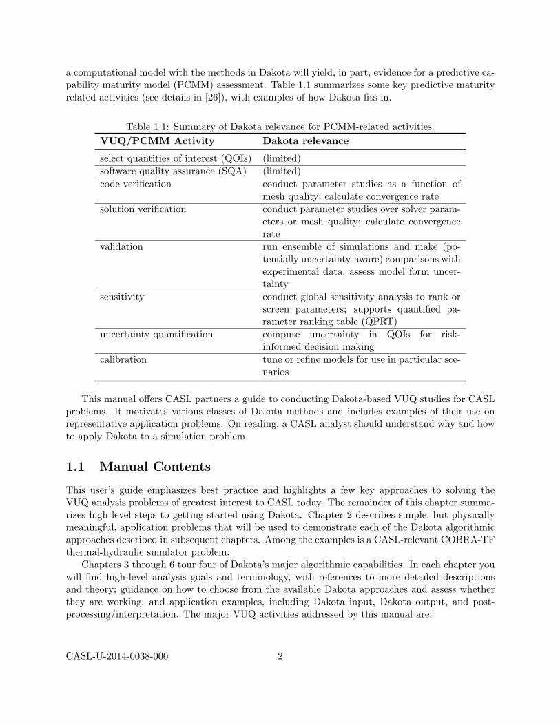
a computational model with the methods in Dakota will yield, in part, evidence for a predictive ca-pability maturity model (PCMM) assessment. Table 1.1 summarizes some key predictive maturityrelated activities (see details in [26]), with examples of how Dakota fits in.
Table 1.1: Summary of Dakota relevance for PCMM-related activities.VUQ/PCMM Activity Dakota relevance
select quantities of interest (QOIs) (limited)software quality assurance (SQA) (limited)code verification conduct parameter studies as a function of
mesh quality; calculate convergence ratesolution verification conduct parameter studies over solver param-
eters or mesh quality; calculate convergencerate
validation run ensemble of simulations and make (po-tentially uncertainty-aware) comparisons withexperimental data, assess model form uncer-tainty
sensitivity conduct global sensitivity analysis to rank orscreen parameters; supports quantified pa-rameter ranking table (QPRT)
uncertainty quantification compute uncertainty in QOIs for risk-informed decision making
calibration tune or refine models for use in particular sce-narios
This manual offers CASL partners a guide to conducting Dakota-based VUQ studies for CASLproblems. It motivates various classes of Dakota methods and includes examples of their use onrepresentative application problems. On reading, a CASL analyst should understand why and howto apply Dakota to a simulation problem.
1.1 Manual Contents
This user’s guide emphasizes best practice and highlights a few key approaches to solving theVUQ analysis problems of greatest interest to CASL today. The remainder of this chapter summa-rizes high level steps to getting started using Dakota. Chapter 2 describes simple, but physicallymeaningful, application problems that will be used to demonstrate each of the Dakota algorithmicapproaches described in subsequent chapters. Among the examples is a CASL-relevant COBRA-TFthermal-hydraulic simulator problem.
Chapters 3 through 6 tour four of Dakota’s major algorithmic capabilities. In each chapter youwill find high-level analysis goals and terminology, with references to more detailed descriptionsand theory; guidance on how to choose from the available Dakota approaches and assess whetherthey are working; and application examples, including Dakota input, Dakota output, and post-processing/interpretation. The major VUQ activities addressed by this manual are:
CASL-U-2014-0038-000 2

• Parameter Studies and Sensitivity Analysis: Dakota parameter studies automate typ-ical parameter variation studies such as running the model at a tensor grid of parametervalues or varying them 1%, 5%, 10% from a nominal value. Sensitivity analysis determinesmodel parameters most influential on quantities of interest (responses). This can be used torank the influence of parameters, as in a Quantified Parameter Ranking Table (QPRT) [26],or screen/down-select to a tractable number of free parameters for follow-on analyses. SeeChapter 3, Sensitivity Analysis for an overview of parameter studies, global sensitivity analy-sis methods and metrics, and a demonstration of using Dakota to perform parameter ranking.
• Surrogate Models: Any of the Dakota studies described can be conducted directly on acomputational model or with surrogate model indirection. Surrogate models are inexpensiveapproximate models that are intended to capture the salient features of an expensive high-fidelity model. In this manual and the Dakota context, surrogate models are not basedon simplifying physical assumptions. Rather they are response surface models constructedautomatically by Dakota based on empirical samples of the true simulation’s input/outputbehavior. For example, in CASL one might run costly CFD simulations at a set of designpoints in a parameter space and then have Dakota build an algebraic Kriging model on theQOI data for use in optimization. Chapter 4 has an overview of the most commonly usedsurrogate models, which can smooth noisy model responses, or reduce computational cost. Onreading it, you will be able to create Dakota studies that automatically run a computationalmodel, generate a response surface model, and evaluate it in the context of another Dakotastudy.
• Calibration: Dakota provides capabilities for automatically tuning model parameters tobest match experimental (or high-fidelity model) data. This process is also known as pa-rameter estimation, calibration, data assimilation, or model inversion to update knowledgeof parameter values based on additional data. A CASL example would be tuning crud chem-istry reaction rates to match experimental data. Approaches yielding single point estimatesof parameters are described in Chapter 5, Optimization and Deterministic Calibration, whileBayesian methods resulting in a probability distribution for the unknown parameters arecovered in Section 6.2, Bayesian Model Calibration.
• Design Optimization: Adjusting model parameters to meet desired performance criteriawhile satisfying other constraints. For example, determine optimal shape to minimize vi-bration, or design mixing vanes to minimize crud formation. Chapter 5, Optimization andDeterministic Calibration will help you choose from among Dakota optimization methodsbased on problem characteristics and your specific optimization goals.
• Uncertainty Quantification (UQ): Model predictions with quantified uncertainty supportvalidation and follow-on decision making. UQ methods accept characterizations of input pa-rameter uncertainty and run the computational model to compute the resulting uncertaintieson response quantities of interest. UQ methods, which yield statistics on QOIs (mean, stan-dard deviation, distribution, range), are described in Chapter 6, Uncertainty Quantification.
This guide selectively focuses on two to three ways to execute each type of VUQ analysisdepending on goals and problem characteristics. The approaches included have worked well inpractice on a broad range of problems in computational science and engineering. When challenges
CASL-U-2014-0038-000 3

are encountered, many alternative and advanced methods that may perform better are available inDakota.
The manual concludes with a realistic thermal-hydraulics example from a CASL “ProgressionProblem” in Chapter 7, COBRA-TF VUQ Studies. The example demonstrates a VUQ activity flowfrom initial parameter studies, through sensitivity analysis for parameter screening, to calibrationon a reduced parameter set. Construction of the surrogate utilized in model calibration as asubstitute for more costly direct COBRA-TF calculations is also illustrated.
Additional Resources
This user’s guide is not an exhaustive guide to Dakota’s capabilities. It is a high-level supplementto other Dakota and VUQ resources. Users reaching its extent should consult:
• The Dakota User’s Manual [1]: a more complete summary of Dakota capabilities from get-ting started through advanced methods (http://dakota.sandia.gov/docs/dakota/5.4/Users-5.4.pdf);
• The Dakota Reference Manual [2]: extensive guidance on valid keywords to use in a Dakota in-put file to specify a Dakota study (http://dakota.sandia.gov/docs/dakota/5.4/html-ref/index.html);
• The directories dakota/examples and dakota/test included with Dakota distributions whichcontain examples of input files referenced in the documentation and many more (also availableat https://software.sandia.gov/trac/dakota/browser/tags/5.4/examples and https://software.sandia.gov/trac/dakota/browser/tags/5.4/test);
• The Dakota Theory Manual [3] (http://dakota.sandia.gov/docs/dakota/5.4/Theory-5.4.pdf) and research publications available at http://dakota.sandia.gov/publications.html: detailed background on algorithmic approaches developed directly in Dakota to tacklechallenging science and engineering analyses; and
• Publications referenced throughout all the above.
This document refers to Dakota 5.4 and its documentation; newer versions may be available onthe Dakota website. This guide for Dakota usage in CASL aims to be generic and thus does notsupplant any domain-specific best practices or guidance for performing VUQ-related studies.
1.2 Getting Started with Dakota
The remainder of this manual largely focuses on selecting and applying Dakota methods and un-derstanding the results. This section surveys at a higher level some prerequisites for using Dakota,with references to additional resources for help.
Know Why to Use Dakota
Understanding your simulation’s characteristics, your VUQ analysis goals, and Dakota’s relevancein achieving them are critical first steps. These likely seem obvious, but are crucial in order to selectfrom the many available methods in Dakota. This guide aims to address this background by offering
CASL-U-2014-0038-000 4

a high-level introduction to some key analysis methods, their application, and benefits. Otherresources to understanding Dakota’s applicability include training materials, publicity materials,and publications on the Dakota website http://dakota.sandia.gov, as well as the Dakota User’sManual [1].
Access the Software and Other Resources
Dakota: Dakota is available to CASL partners as part of the Virtual Environment for Reactor Ap-plications (VERA). It can be checked out via git clone from casl-dev.ornl.gov:/git-root/Dakota.Dakota is also distributed with VERA releases under Trilinos/packages/TriKota/Dakota. Ex-amples of Dakota applied to CASL problems are evolving. These are archived in milestonereports and protected in the VERA software in the VUQDemos suite, available via git clonefrom casl-dev.ornl.gov:/git-root/VUQDemos. Dakota also has a public download site http://dakota.sandia.gov/download.html, which may be useful for CASL partners without readyaccess to the VERA development environment at Oak Ridge National Laboratory (ORNL).
This Manual and Examples: Examples from this manual, including input, output, auxiliiarydata files, and scripts are available from the CASL Git repository atcasl-dev.ornl.gov:/git-root/VUQDemos/CaslDakotaManual. The LATEXsource and images arealso included.
Help Resources: For help beyond this manual and the documents referenced herein, see theDakota website: http://dakota.sandia.gov. It includes software downloads, documentation,publications, and training materials. It also has guidance on seeking general help with Dakotavia the dakota-users mailing list ([email protected]). CASL-specific issuesshould be directed to [email protected].
How to Interact with Dakota
An overall Dakota analysis process is depicted in Figure 1.1. The specification of the VUQ analysisproblem to Dakota is given in the text-based Dakota input file, including the method (algorithm)which dictates how Dakota generates parameter sets at which to run the user’s simulation. AsDakota runs, it will iteratively evaluate the simulation at these parameter sets by running a user-provided analysis driver and collecting corresponding quantities of interest output by the simulationworkflow. When complete, the Dakota executable will produce console text output and tabulardata with VUQ results for subsequent analysis.
Interface Dakota to the Simulation
Dakota requires an analysis driver to communicate with the computational model. The contractfor this Dakota/simulation interface is straightforward: it must be an automated workflow thataccepts Dakota parameters as input from a text file, runs the simulation in a batch/non-interactivemode, and produces responses (quantities of interest derived from simulation output) in a text filefor consumption by Dakota.
As Dakota runs, it will determine values of parameters for which response data is needed. Whenready to evaluate the simulation at such a parameter set, Dakota will write a “parameters file” withthe values of the variables. Dakota will then invoke the specified analysis driver, represented by thedashed blue box in Figure 1.1. This analysis driver must implement the automated process that
CASL-U-2014-0038-000 5

Dakota Text Input
File
Dakota Output:
Text and Tabular Data
Simulation
(physics model) Code
Input
Code
Output
Dakota Parameters
File variables
Preprocessing User-supplied
automatic post-
processing
Analysis Driver interface
QOIs in Dakota
Results File responses
Dakota Executable method
Figure 1.1: Components of a Dakota study, including Dakota input and output, and interface to acomputational model (simulation).
takes a Dakota parameters file as input and produces a Dakota results file as output. Typicallythis driver is a script which includes preprocessing, running the code, and postprocessing to extractQOIs from simulation output. When the driver completes, Dakota requires the “results file” tocontain the quantities of interest resulting from running the simulation at the specified parametervalues.
Additional resources for creating and running a Dakota/simulation workflow include:
• High level guidance in “User Supplied Simulation Code Examples” in the Dakota Tutorial inthe Dakota User’s Manual [1], with more details in the “Advanced Simulation Code Interfaces”chapter, together with example code in dakota/examples/script interfaces.
• Considerations for having Dakota manage concurrent simulation runs in parallel, as this is acommon need. Managing parallel concurrency locally, within queue, and out of queue, includ-ing batch submission and later retrieval are addressed by the Dakota User’s Manual, “Appli-cation Parallelism Use Cases”, together with examples in dakota/examples/parallelism.
• CASL-specific Dakota workflows with COBRA-TF and Insilico, demonstrated in the abovereferenced VUQDemos.
Understand Dakota Input Files
Once an interface is constructed between Dakota and the simulation, one may readily apply anyDakota method by simply changing the input file. Dakota input files are simple plain text files withsix categories of information that can appear (some are optional and some may appear multipletimes in advanced studies). Four of these are indicated notionally in Figure 1.1:
• strategy (not depicted): overall control of Dakota methods and tabular output data.
CASL-U-2014-0038-000 6

• method: specifies the iterative analysis method being run on the model, for example Latinhypercube sampling or gradient-based parameter estimation.
• variables: characterization of the model parameters Dakota is varying in the study, such aslognormal uncertain or continuous design, together with supplementary fixed (state) param-eters.
• responses: quantities of interest returned to Dakota for analysis.
• interface: the simulation workflow mapping variables to responses in an automated way;typically a script that orchestrates this workflow.
• model (not depicted): a container encapsulating a set of variables, interface, and responses forpresentation to a method; useful for specifying that a surrogate model should be automaticallyconstructed to serve as a proxy for an expensive computational model.
This guide shows and explains a number of examples of input files which configure Dakotato conduct various kinds of iterative analyses. They can be taken verbatim from the text toconduct Dakota studies and will also be available from CASL records systems when this manual ispublished. Additional examples are available in the various Dakota manuals and with the Dakotasoftware itself. Specific guidance on individual Dakota keywords is available in the Dakota ReferenceManual [2], which can help when trying to determine how to configure Dakota for a new kind ofstudy.
Understand Dakota Results
This document offers an introduction to Dakota output, including log file output and tabular datato understand the results of studies. Often this data must be interpreted or post-processed withexternal tools to be useful in a decision making context. Examples are included in this manual todemonstrate this.
1.3 Acknowledgments
This CASL/Dakota manual borrows heavily from the Dakota 5.4 User’s Manual [1]. We heartilythank the authors of the most recent version of that document: Brian M. Adams, Lara E. Bauman,William J. Bohnhoff, Keith R. Dalbey, John P. Eddy, Mohamed S. Ebeida, Michael S. Eldred,Patricia D. Hough, Kenneth T. Hu, John D. Jakeman, Laura P. Swiler, and Dena M. Vigil.
Dakota’s use of the Quantification of Uncertainty for Estimation, Simulation, and Optimization(QUESO) library is facilitated through close interaction with its developers at the University ofTexas at Austin. Ernesto E. Prudencio, Nicholas Malaya, and Damon McDougall have kindlyprovided examples and test problems implemented in QUESO.
We also appreciate the efficient implementation of code changes to COBRA-TF made byNoel K. Belcourt to expose code parameters to Dakota needed to drive the various COBRA-TFparameter studies described in this manual.
We appreciate the valuable feedback provided by several reviewers of this manual, includingPatty Hough, Vince Mousseau, Rod Schmidt, and Dena Vigil.
This research was supported by the Consortium for Advanced Simulation of Light Water Re-actors (http://www.casl.gov), an Energy Innovation Hub (http://www.energy.gov/hubs) for
CASL-U-2014-0038-000 7

Modeling and Simulation of Nuclear Reactors under U.S. Department of Energy Contract No. DE-AC05-00OR22725. Sandia National Laboratories (SNL), North Carolina State University (NCSU),and Los Alamos National Laboratory (LANL) are core CASL partners.
CASL-U-2014-0038-000 8

Chapter 2
Application Example Problems
This chapter describes representative, though simplified, application problems that will be used todemonstrate various Dakota approaches. Each of the three application examples has strengths tohelp bridge abstract Dakota concepts and guidance throughout the remainder of this manual toconcrete practice:
• Cantilever beam: A simple static mechanics analysis where prescribed geometry, materialproperties, and loads on a cantilevered beam map to to quantities of interest such as weight,displacement, and stress. The physical meaning is intuitive, the physics equations have asimple algebraic form, and a simulator for it is included with Dakota, along with severalexample input files. Each Dakota analysis technique in Chapters 3 through 6 includes aworked example using the cantilever beam problem.
• General linear model: A model with closed algebraic form specifically designed to supportalgorithm and code verification, i.e., to verify that VUQ algorithms are working as expected.This example consists of a linear mapping from model parameters to responses, with anadditive noise term. It is used to verify the performance of Bayesian calibration methods inSection 6.2.
• COBRA-TF thermal-hydraulics: A coupled physics, single assembly reactor model prob-lem simulated with CASL’s COBRA-TF thermal-hydraulics code. The most physically realis-tic example, this problem demonstrates VUQ infrastructure for varying model form and otherparameters, running a computational model, and distilling quantities of interest from codeoutput. This example is the focus of Chapter 7, where it is used to demonstrate parameterscreening, calibration, and surrogate construction.
2.1 Cantilever beam
The cantilever beam example problem is adapted from the reliability-based design optimizationliterature [36], [42]. The uniform cantilever beam is shown in Figure 2.1, with a left anchor and afixed length L = 100in. The beam width and thickness are parameterized by w and t, respectively.The free end of the beam is subject to horizontal load X and vertical load Y .
Given Young’s elastic modulus E, the simplified algebraic physics equations used to model the
CASL-U-2014-0038-000 9
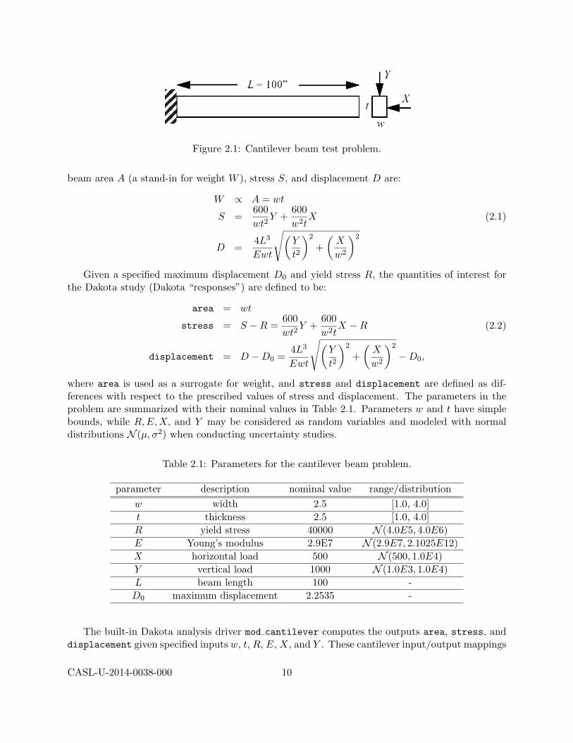
Figure 2.1: Cantilever beam test problem.
beam area A (a stand-in for weight W ), stress S, and displacement D are:
W ∝ A = wt
S =600wt2
Y +600w2t
X (2.1)
D =4L3
Ewt
√(Y
t2
)2
+(X
w2
)2
Given a specified maximum displacement D0 and yield stress R, the quantities of interest forthe Dakota study (Dakota “responses”) are defined to be:
area = wt
stress = S −R =600wt2
Y +600w2t
X −R (2.2)
displacement = D −D0 =4L3
Ewt
√(Y
t2
)2
+(X
w2
)2
−D0,
where area is used as a surrogate for weight, and stress and displacement are defined as dif-ferences with respect to the prescribed values of stress and displacement. The parameters in theproblem are summarized with their nominal values in Table 2.1. Parameters w and t have simplebounds, while R,E,X, and Y may be considered as random variables and modeled with normaldistributions N (µ, σ2) when conducting uncertainty studies.
Table 2.1: Parameters for the cantilever beam problem.
parameter description nominal value range/distributionw width 2.5 [1.0, 4.0]t thickness 2.5 [1.0, 4.0]R yield stress 40000 N (4.0E5, 4.0E6)E Young’s modulus 2.9E7 N (2.9E7, 2.1025E12)X horizontal load 500 N (500, 1.0E4)Y vertical load 1000 N (1.0E3, 1.0E4)L beam length 100 -D0 maximum displacement 2.2535 -
The built-in Dakota analysis driver mod cantilever computes the outputs area, stress, anddisplacement given specified inputs w, t, R, E, X, and Y . These cantilever input/output mappings
CASL-U-2014-0038-000 10

will be utilized throughout this manual to illustrate the application of core CASL VUQ technologieswith Dakota. In Section 3.2, the sensitivity of the quantities of interest with respect to the inputparameters is assessed to rank their importance and exercise the model.
Then, in Sections 4.1.1 and 4.2.1, response surface models (surrogates) for the parameter toresponse mapping are generated based on a small number of sampled runs of cantilever. Thisemulates the practical process one must use when models are costly. In Section 5.2, a deterministicdesign optimization problem is solved to design the beam geometry. The goal is to minimize theweight (or equivalently, the cross-sectional area) of the beam subject to a displacement constraintand a stress constraint. The parameters R, E, X, and Y are fixed at their nominal values and thedeterministic design problem is given by
minimize area = wt
subject to stress = S −R ≤ 0 (2.3)displacement = D −D0 ≤ 01.0 ≤ w ≤ 4.01.0 ≤ t ≤ 4.0
In Section 5.2.1, the cantilever beam is calibrated to synthetic experimental data for area, stress,and displacement, to find the values of w, t, and E yielding best agreement with the data. Finally,when considered for uncertainty quantification in Chapter 6, the design variables are fixed attheir nominal or optimal values, and the Dakota study is conducted over the normally-distributeduncertain parameters R, E, X, and Y . This yields estimates of the mean, standard deviation, andoverall distribution of the quantities of interest.
2.2 General Linear Model Verification Test Suite
Whereas most CASL codes exhibit a nonlinear input-output relation, linearly parameterized prob-lems serve an important role for algorithm and code verification. These uses include the following:
• They provide a hierarchy of models, which can be used to test the convergence of Bayesianmodel calibration algorithms through comparison with analytic solutions.
• They provide a regime to test of the accuracy of uncertainty propagation algorithms sinceone can employ analytic relations between input and output densities.
• They facilitate the testing of algorithms for heavy-tailed distributions.
• They provide a framework for analytically testing algorithms to construct Sobol global sen-sitivity indices (described in Section 3.1.2).
The family of linear models described in this section is used to verify the performance of Bayesiancalibration methods in Section 6.2. A high-level overview of the problem appears here, with addi-tional details in Appendix A. A simulator implementing this problem is available on request fromthe authors.
We employ the linear regression model
Y = Gβ + ε(λ, φ). (2.4)
CASL-U-2014-0038-000 11
as a test problem for verifying the Bayesian calibration capabilities in Dakota, which currentlyinclude Quantification of Uncertainty for Estimation, Simulation, and Optimization (QUESO) andDifferential Evolution with Self-Adaptive Randomized Subspace Sampling (via the DREAM soft-ware package). In this model Y is the N -dimensional vector of noisy observations of the quantity ofinterest. The N ×Nβ matrix G is known and the Nβ components of the vector β are unknown re-gression parameters to be estimated. The N -dimensional random variable ε represents the randommeasurement noise in the observations. The measurement noise is normally distributed with meanzero and N ×N covariance matrix R(φ)/λ. The precision (inverse variance) λ of the ε process isa positive scalar and the permissible values for the correlation structural parameter φ depend onthe type of correlation being considered as discussed below.
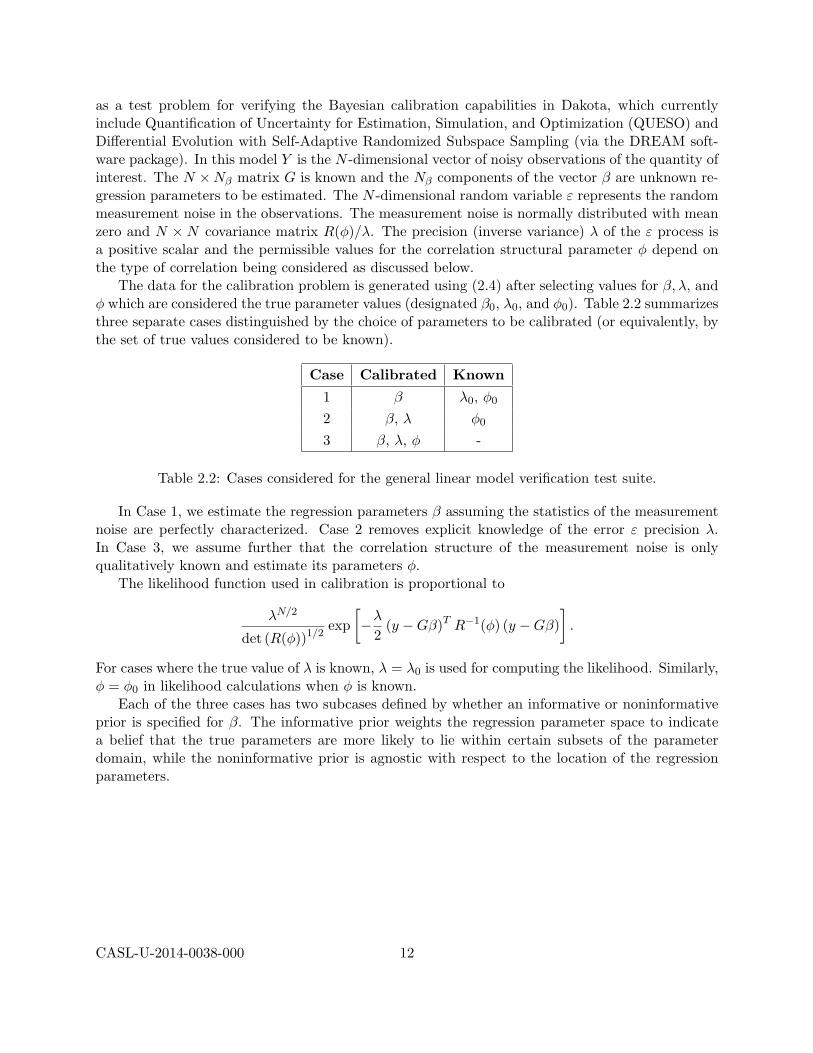
The data for the calibration problem is generated using (2.4) after selecting values for β, λ, andφ which are considered the true parameter values (designated β0, λ0, and φ0). Table 2.2 summarizesthree separate cases distinguished by the choice of parameters to be calibrated (or equivalently, bythe set of true values considered to be known).
Case Calibrated Known
1 β λ0, φ0
2 β, λ φ0
3 β, λ, φ -
Table 2.2: Cases considered for the general linear model verification test suite.
In Case 1, we estimate the regression parameters β assuming the statistics of the measurementnoise are perfectly characterized. Case 2 removes explicit knowledge of the error ε precision λ.In Case 3, we assume further that the correlation structure of the measurement noise is onlyqualitatively known and estimate its parameters φ.
The likelihood function used in calibration is proportional to
λN/2
det (R(φ))1/2exp
[−λ
2(y −Gβ)T R−1(φ) (y −Gβ)
].
For cases where the true value of λ is known, λ = λ0 is used for computing the likelihood. Similarly,φ = φ0 in likelihood calculations when φ is known.
Each of the three cases has two subcases defined by whether an informative or noninformativeprior is specified for β. The informative prior weights the regression parameter space to indicatea belief that the true parameters are more likely to lie within certain subsets of the parameterdomain, while the noninformative prior is agnostic with respect to the location of the regressionparameters.
CASL-U-2014-0038-000 12
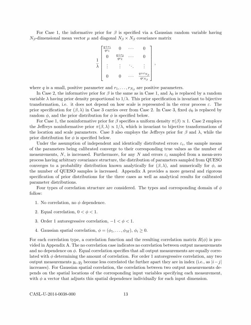
For Case 1, the informative prior for β is specified via a Gaussian random variable havingNβ-dimensional mean vector µ and diagonal Nβ ×Nβ covariance matrix
1λ
q+r1qr1
0 · · · 0
0 q+r2qr2
· · · 0
......
. . ....
0 0 · · · q+rNβqrNβ
,
where q is a small, positive parameter and r1, . . . , rNβ are positive parameters.In Case 2, the informative prior for β is the same as in Case 1, and λ0 is replaced by a random
variable λ having prior density proportional to 1/λ. This prior specification is invariant to bijectivetransformation, i.e. it does not depend on how scale is represented in the error process ε. Theprior specification for (β, λ) in Case 3 carries over from Case 2. In Case 3, fixed φ0 is replaced byrandom φ, and the prior distribution for φ is specified below.
For Case 1, the noninformative prior for β specifies a uniform density π(β) ∝ 1. Case 2 employsthe Jeffreys noninformative prior π(β, λ) ∝ 1/λ, which is invariant to bijective transformations ofthe location and scale parameters. Case 3 also employs the Jeffreys prior for β and λ, while theprior distribution for φ is specified below.
Under the assumption of independent and identically distributed errors εi, the sample meansof the parameters being calibrated converge to their corresponding true values as the number ofmeasurements, N , is increased. Furthermore, for any N and errors εi sampled from a mean-zeroprocess having arbitrary covariance structure, the distribution of parameters sampled from QUESOconverges to a probability distribution known analytically for (β, λ), and numerically for φ, asthe number of QUESO samples is increased. Appendix A provides a more general and rigorousspecification of prior distributions for the three cases as well as analytical results for calibratedparameter distributions.
Four types of correlation structure are considered. The types and corresponding domain of φfollow:
1. No correlation, no φ dependence.
2. Equal correlation, 0 < φ < 1.
3. Order 1 autoregressive correlation, −1 < φ < 1.
4. Gaussian spatial correlation, φ = (φ1, . . . , φM ), φi ≥ 0.
For each correlation type, a correlation function and the resulting correlation matrix R(φ) is pro-vided in Appendix A. The no correlation case indicates no correlation between output measurementsand no dependence on φ. Equal correlation specifies that all output measurements are equally corre-lated with φ determining the amount of correlation. For order 1 autoregressive correlation, any twooutput measurements yi, yj become less correlated the further apart they are in index (i.e., as |i−j|increases). For Gaussian spatial correlation, the correlation between two output measurements de-pends on the spatial locations of the corresponding input variables specifying each measurement,with φ a vector that adjusts this spatial dependence individually for each input dimension.
CASL-U-2014-0038-000 13

The prior distribution for φ is taken to be uniform on the allowable domain for φ in the equaland autoregressive correlation cases. For Gaussian spatial correlation, assume the M inputs x arerestricted by the bounds `i ≤ xi ≤ ui for i = 1, . . . ,M . The prior distribution π(φ) for φ is givenby
π(φ) ∝M∏i=1
[ρi(φi)]aρ [1− ρi(φi)]bρ−1 χ[0,∞)(φi) ,
where ρi(φ) = exp[−φ(ui − `i)2/4
]for i = 1, . . . ,M , (aρ, bρ) = (1, 0.1), and χ[0,∞)(φ) is the
characteristic function taking value 1 for φ ≥ 0 and 0 for φ < 0.
2.3 COBRA-TF Thermal-Hydraulics Simulation Problem
This section provides an overview of COBRA-TF and a particular thermal-hydraulics simulationproblem, CASL VERA Progression Problem 6. An end-to-end demonstration of Dakota methodsusing this COBRA-TF model is in Chapter 7, COBRA-TF VUQ Studies. The full Dakota/COBRA-TF example is available in the CASL software repositories. Details on accessing it are provided inAppendix B.
2.3.1 COBRA-TF Simulator Overview
COBRA-TF is a thermal-hydraulic (T/H) simulation code designed for light water reactor (LWR)analysis) [5]. COBRA-TF has a long lineage back to the original COBRA computer code developedin 1980 by Pacific Northwest Laboratory, under sponsorship of the Nuclear Regulatory Commis-sion (NRC). The original COBRA began as a thermal-hydraulic rod-bundle analysis code, butsubsequent versions have updated and expanded over the past several decades to cover almost allsteady-state and transient analyses of both pressurized water reactors (PWRs) and boiling waterreactors (BWRs). COBRA-TF is currently developed and maintained by the Reactor Dynamicsand Fuel Management Group (RDFMG) at the Pennsylvania State University (PSU). Additionalinformation can be found at the RDFMG website, http://www.mne.psu.edu/RDFMG/index.html.
COBRA-TF includes a wide range of thermal-hydraulic models important to LWR safety analy-sis including flow regime dependent two-phase wall heat transfer, inter-phase heat transfer and drag,droplet breakup, and quench-front tracking. COBRA-TF also includes several internal models tohelp facilitate the simulation of realistic fuel assemblies. These models include spacer grid models,a fuel rod conduction model, and built-in material properties for both the structural materials andthe coolant (i.e., steam tables).
COBRA-TF uses a two-fluid, three-field representation of the two-phase flow. The equationsand fields solved are:
• Continuous vapor (mass, momentum and energy)
• Continuous liquid (mass, momentum and energy)
• Entrained liquid drops (mass and momentum)
• Non-condensable gas mixture (mass)
CASL-U-2014-0038-000 14
Reasons for selecting COBRA-TF as the primary T/H solver in the VERA core simulator include:reasonable run-times compared to CFD (although CFD will be available as an option), the factthat it is being actively developed and supported by PSU, ability to support future applications ofVERA such as transient safety analysis and BWR and SMR applications.
2.3.2 COBRA-TF test problem description
The thermal-hydraulics application example problem used in this manual is a coupled single assem-bly problem known in CASL as Progression Problem 6 [31]. It simulates a single PWR assemblybased on the dimensions and state conditions of Watts Bar Unit 1 Cycle 1. The dimensions for theassembly are identical to AMA Progression Benchmarks “Problem 3” and “Problem 6”. Problems3 and 6 are identical, except that Problem 3 is at Hot Zero Power (HZP) and has no T/H feedback,and Problem 6 is at Hot Full Power (HFP) and includes T/H feedback. The test case was run ata boron concentration of 1300 ppm and a 100% power level.
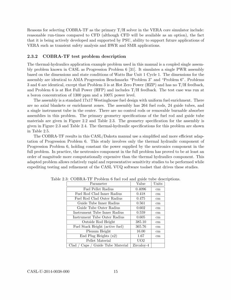
The assembly is a standard 17x17 Westinghouse fuel design with uniform fuel enrichment. Thereare no axial blankets or enrichment zones. The assembly has 264 fuel rods, 24 guide tubes, anda single instrument tube in the center. There are no control rods or removable burnable absorberassemblies in this problem. The primary geometry specifications of the fuel rod and guide tubematerials are given in Figure 2.2 and Table 2.3. The geometry specification for the assembly isgiven in Figure 2.3 and Table 2.4. The thermal-hydraulic specifications for this problem are shownin Table 2.5.
The COBRA-TF results in this CASL/Dakota manual use a simplified and more efficient adap-tation of Progression Problem 6. This study involves only the thermal hydraulic component ofProgression Problem 6, holding constant the power supplied by the neutronics component in thefull problem. In practice, the neutronics component in the full problem has proved to be at least anorder of magnitude more computationally expensive than the thermal hydraulics component. Thisadapted problem allows relatively rapid and representative sensitivity studies to be performed whileexpediting testing and refinement of the CASL VUQ software toolset that drives these studies.
Table 2.3: COBRA-TF Problem 6 fuel rod and guide tube descriptions.Parameter Value Units
Fuel Pellet Radius 0.4096 cmFuel Rod Clad Inner Radius 0.418 cmFuel Rod Clad Outer Radius 0.475 cm
Guide Tube Inner Radius 0.561 cmGuide Tube Outer Radius 0.602 cm
Instrument Tube Inner Radius 0.559 cmInstrument Tube Outer Radius 0.605 cm
Outside Rod Height 385.10 cmFuel Stack Height (active fuel) 365.76 cm
Plenum Height 16.00 cmEnd Plug Heights (x2) 1.67 cm
Pellet Material UO2Clad / Caps / Guide Tube Material Zircaloy-4
CASL-U-2014-0038-000 15

Figure 2.2: COBRA-TF Problem 6 fuel rod diagram.
Figure 2.3: COBRA-TF Problem 6 assembly layout showing guide tubes and instrument tubeplacement.
CASL-U-2014-0038-000 16

Table 2.4: COBRA-TF Problem 6 assembly specification.Parameter Value UnitsRod Pitch 1.26 cm
Assembly Pitch 21.5 cmInter-Assembly Half Gaps 0.04 cm
Geometry 17x17Number of Fuel Rods 264
Number of Guide Tubes 24Number of Instrument Tubes 1
Table 2.5: COBRA-TF Problem 6 nominal thermal-hydraulic conditions.Parameter Value Units
Inlet Temperature 559 degrees FSystem Pressure 2250 psia
Rated Flow (100% flow) 0.6824 Mlb/hrRated Power (100% power) 17.67 MWt
2.3.3 VUQ Parameters in COBRA-TF Problem 6
At present, CASL VUQ workflows support COBRA-TF simulation parameter variation via twomechanisms. The first allows Dakota to seamlessly integrate with the VERA Common Input toolsuite to perturb any parameters exposed to a user. The second path targets specific code parametersin the thermal hydraulics code that represent all physical phenomena modeled with closure laws inCOBRA-TF. These “VUQ parameters” are not exposed to a normal user but are instead exposedto Dakota using an auxiliary input file. The principle is that most analyst users should only perturbinput data appearing in the VERA text input file, while advanced VUQ users may need to perturbmore advanced parameters such as closure laws. The COBRA-TF studies presented in Chapter 7use the second mode of parameter variation, i.e. perturbing code parameters via the auxiliary file.
For each parameter, Dakota is able to apply perturbations representing combined shift andscaling, e.g. for an arbitrary parameter p, Dakota can specify values for kp and kap which are usedas follows:
p = kp ∗ p+ kap (2.5)
The relevant parameters identified by Noel Belcourt and the COBRA-TF code team along withbrief descriptions taken from [32] are summarized in Table 2.6. The entries containing “(??)” intheir description were not documented in [32] but instead were inferred from the COBRA-TF sourcecode.
CASL-U-2014-0038-000 17

Table 2.6: Relevant COBRA-TF thermal-hydraulic code parameters identified by PIRT study.cd Pressure loss coefficient of spacer in sub-channel
cdfb Pressure loss coefficient for sub-channel flow blockage (??)cond Thermal conductivity of radial heat transfereta Fraction of vapor generation rate coming from the entrained liquid field
gama New time vapor generation rate in sub-channelql∗ Heat transfer rate to liquid in sub-channel
qliht Heat transfer due to drop impact (??)qradd Radiative heat transfer rate from wall to entrained liquidqradv Radiative heat transfer rate from wall to vaporqv∗ Heat transfer rate to liquid in sub-channel
qvapl Incremental heat transferred from grid to vapor (??)rodqq Externally supplied heat rate of current rod at current time step (axially averaged)sdent Deposition mass flow rate in sub-channelsent Entrainment mass flow rate in sub-channelsphts Specific heat of radial heat transfertmasg Loss of mass of non-condensable gas in local axial fluid continuity cell
due to mixing and void drift to radially adjacent fluid cellstmasl Loss of mass of continuous liquid in local axial fluid continuity cell
due to mixing and void drift to radially adjacent fluid cellstmasv Loss of mass of vapor in local axial fluid continuity cell
due to mixing and void drift to radially adjacent fluid cellstmome Loss of momentum of droplets in sub-channel
due to mixing and void drift to radially adjacent fluid cellstmoml Loss of momentum of continuous liquid in sub-channel
due to mixing and void drift to radially adjacent fluid cellstmomv Loss of momentum of vapor in sub-channel
due to mixing and void drift to radially adjacent fluid cellstnrgl Loss of enthalpy of liquid in local axial fluid continuity due to mixing
and void drift to radially adjacent fluid cellstnrgv Loss of enthalpy of vapor in local axial fluid continuity due to mixing
and void drift to radially adjacent fluid cellswkr Lateral gap pressure loss coefficientxk Vertical interfacial drag coefficient between the continuous liquid and vapor phases
xkes Sink interfacial drag coefficient between the liquid and vapor phasesxkge Vertical interfacial drag coefficient between the entrained liquid and vapor phasesxkl Transverse interfacial drag coefficient between the continuous liquid and vapor phasesxkle Transverse interfacial drag coefficient between the entrained liquid and vapor phasesxkvls Sink interfacial drag coefficient between the continuous liquid and vapor phases
xkwew Transverse entrained liquid form loss coefficientxkwlw Transverse liquid wall drag coefficientxkwlx Vertical liquid wall drag coefficientxkwvw Transverse vapor wall drag coefficientxkwvx Vertical vapor wall drag coefficient
CASL-U-2014-0038-000 18

Chapter 3
Sensitivity Analysis
Broadly, the primary goal of sensitivity analysis is to determine which input parameters mostinfluence computational model responses, or deterministic quantities of interest. A ranked list ofparameter influences can focus resources for data gathering or model/code development, or canmake calibration, optimization, or uncertainty quantification more tractable over a reduced set ofparameters. In a post-optimization role, sensitivity information is useful is determining whether ornot the response functions are robust with respect to small changes in the optimum design point.The Dakota sensitivity analysis studies recommended in this chapter have important secondarybenefits as well: (1) they can help identify key model characteristics such as smoothness, nonlineartrends, and robustness to enable selection of suitable Dakota methods for follow-on studies; and(2) some yield sampling designs that can be used to construct the surrogate models described inChapter 4 for subsequent analyses.
In the CASL context, a phenomena identification and ranking table (PIRT) might help identifythe superset of parameters to consider in a sensitivity analysis study. Then the relative parameterrankings resulting from a Dakota-driven sensitivity study form the basis of a quantitative PIRT,or QPRT. These results could also help prioritize model development or data gathering, or identifyinsensitive parameters to omit from calibration or UQ studies.
3.1 Terminology
This section introduces key sensitivity analysis terminology and defines the metrics typically usedto assign relative ranks to parameter influences on a response.
3.1.1 Local Versus Global Sensitivity
Dakota primarily focuses on sensitivity analysis in a global sense, i.e., over the whole valid parameterdomain. We contrast that here with more traditional local or partial derivative-based sensitivityanalysis.
Local Sensitivity: In some instances, the term sensitivity analysis is used in a local senseto denote the computation of response derivatives with respect to parameters at a point. Theselocal derivatives can then be used to make design decisions or rank parameter influences. Dakotasupports this type of study through numerical finite-differences or retrieval of analytic gradientscomputed within the analysis code. The desired gradient data is specified in the responses section
CASL-U-2014-0038-000 19

of the Dakota input file and the collection of this data at a single point is accomplished through aparameter study method with no steps.
This approach to sensitivity analysis should be distinguished from the activity of augmentinganalysis codes to internally compute derivatives using techniques such as direct or adjoint differen-tiation, automatic differentiation (e.g., ADIFOR), or complex step modifications. These sensitivityaugmentation activities are completely separate from Dakota and are outside the scope of this man-ual. However, once completed, Dakota can utilize these analytic gradients to perform optimization,uncertainty quantification, and related studies more reliably and efficiently. In CASL, some simu-lation codes such as TSUNAMI have adjoint capabilities and can return not only function value,but derivative data to Dakota, enhancing analyses.
Global Sensitivity: In other instances, the term sensitivity analysis is used in a more globalsense to denote the investigation of variability in the response functions over the whole valid rangeof the input parameters. Dakota supports this type of study through computation of response datasets at a series of sample design points in the parameter space. The series of points is typicallydefined using a parameter study or a design and analysis of computer experiments (DACE) design,such as orthogonal arrays or space filling Monte Carlo sampling. These more global approachesto sensitivity analysis can be used to obtain trend data even in situations when gradients areunavailable, unreliable, or not indicative of global trends.
This chapter offers guidance solely on Dakota’s global sensitivity analysis procedures. Usingthem typically consists of:
1. Specifying ranges for each parameter and a sensitivity analysis method in the Dakota input
2. Running Dakota which will:
(a) construct a sampling design in the parameter hypercube;
(b) run the computational model at these points, collecting returned response data; and
(c) calculate and output sensitivity metrics to rank inputs.
3. Post-processing the Dakota-generated parameter/response table with external statistics andvisualization tools to further assess trends and which input factors most strongly influencethe responses
3.1.2 Sensitivity Metrics
Sensitivity metrics output by Dakota are used to assess the relative influence of or rank parameters.The metrics output vary by Dakota method as discussed in Section 3.2, but may include:
• Correlation coefficients: Dakota prints correlation tables with the simple (Pearson), par-tial, and rank (Spearman) correlations between inputs and outputs. These are all boundedbetween -1 and 1 and measure the strength of the linear relationship between the variablesconsidered. These can be useful to get a quick sense of how correlated the inputs are to eachother, and how correlated various outputs are to inputs, but can be misleading for detect-ing nonlinear relationships. For example a model with a perfectly quadratic input/outputrelationship centered at zero would have zero correlation hiding the actual strong nonlinearrelationship.
CASL-U-2014-0038-000 20

The simple correlations are Pearson’s correlation coefficient, which is defined for two factorsw and x (where each of these could represent an input or an output) as:
Corr(w, x) =∑
i(wi − w)(xi − x)√∑i(wi − w)2
∑i(xi − x)2
.
Partial correlation coefficients are similar, but measure correlation while adjusting for theeffects of other variables. For example, in a problem with two inputs and one output wherethe two inputs are highly correlated, the correlation of the second input and the output maybe very low after accounting for the effect of the first input. The rank correlations in Dakotaare obtained using Spearman’s rank correlation. Spearman’s rank is the same as the Pearsoncorrelation coefficient except that it is calculated on the rank data. Rank correlation can bemore informative when responses vary over orders of magnitude. The correlation analyses areexplained further in the Uncertainty Quantification chapter of the Dakota User’s Manual. [1]
• Morris metrics [25] are computed from “elementary effects” based on a sample design oflarge steps around the parameter space. Here each dimension of a M−dimensional inputspace is uniformly partitioned into p levels, creating a grid of pM points x ∈ <M at whichevaluations of the model y(x) might take place. An elementary effect corresponding to inputi is computed by a forward difference
di(x) =y(x+ ∆ei)− y(x)
∆, (3.1)
where ei is the ith coordinate vector, and the step ∆ is typically taken to be large (this is notintended to be a local derivative approximation), e.g., for an input variable scaled to [0, 1],∆ = p
2(p−1) , so the step used to find elementary effects is slightly larger than half the inputrange.
The distribution of elementary effects di over the input space characterizes the effect of inputi on the output of interest. After generating N samples from this distribution, their mean,
µi =1N
N∑j=1
d(j)i , (3.2)
modified mean
µ∗i =1N
N∑j=1
|d(j)i |, (3.3)
(using absolute value) and standard deviation
σi =
√√√√ 1N − 1
N∑j=1
(d
(j)i − µi
)2(3.4)
are computed for each input i. The mean and modified mean give an indication of the overalleffect of an input on the output. Standard deviation indicates nonlinear effects or interactions,since it is an indicator of elementary effects varying throughout the input space.
CASL-U-2014-0038-000 21

• Sobol indices: Dakota can calculate sensitivity indices through Variance-based Decompo-sition (VBD). Variance-based decomposition is a global sensitivity method that summarizeshow the uncertainty in model output can be apportioned to uncertainty in individual inputvariables. VBD uses two primary measures, the main effect sensitivity index Si and the totaleffect sensitivity index Ti. The main effect sensitivity index corresponds to the fraction ofthe total uncertainty in the output, Y , that can be attributed to input xi alone. The totaleffect sensitivity index corresponds to the fraction of the total uncertainty in the output,Y , that can be attributed to input xi and its interactions with other variables. The maineffect sensitivity index compares the variance of the conditional expectation V arXi [E(Y |Xi)]against the total variance V ar(Y ).
Formulas for the indices are:Si =
V arXi [E(Y |Xi)]V ar(Y )
(3.5)
and
Ti =EX−i [V ar(Y |X−i)]
V ar(Y )=V ar(Y )− V arX−i [E(Y |X−i)]
V ar(Y )(3.6)
where Y = f(x) and x−i = (x1, ..., xi−1, xi+1, ..., xM ). The calculation of Si and Ti requiresthe evaluation of M -dimensional integrals which are typically approximated by Monte-Carlosampling.
When using VBD, a rough guide is that variables with main effect indices greater than100/M% are significant as they can be considered to have greater than average effect onoutput variability, barring higher-order interactions. More details on the calculations andinterpretation of the sensitivity indices can be found in [33].
• Main effects show the effects of a single variable, averaging across the effect of other inputvariables. For a full factorial design with each of M inputs taking on p levels, the main effectof input variable xi is calculated at each level k = 1, ..., p it takes on as
mki =
1pM−1
∑x
y(x|xi = xki ).
To calculate main effects with Dakota, one can either use (1) the orthogonal array methodfrom DDACE with the supplementary command main effects, or (2) a grid parameter study,which has to be post-processed to compute main effects in an external statistics tool.
Supplementary Approaches: Running any of the parameter study, design of experiments,or sampling methods allows the user to save the results in a tabular data file, which then can beread into a spreadsheet or statistical package for further analysis. One example of this is the well-known technique of scatter plots, in which the set of samples is projected down and plotted againstone parameter dimension, for each parameter in turn. Scatter plots with a uniformly distributedcloud of points indicate parameters with little influence on the results, whereas scatter plots witha defined shape to the cloud indicate parameters which are more significant. Related techniquesinclude analysis of variance (ANOVA) [27] and main effects analysis, in which parameters havingthe greatest influence on the output are identified from sampling results. Scatter plots and ANOVAmay be accessed through import of Dakota tabular results into external statistical analysis programssuch as R (http://www.r-project.org) and Minitab (http://www.minitab.com).
CASL-U-2014-0038-000 22

3.2 Recommended Methods
This section summarizes a few recommended Dakota sensitivity analysis methods at a high level,shows input file examples, resulting output, and post-processing/visualization approaches that canhelp. The choice of method will depend on the analysis goal and available computational budget.We begin with high-level best practices before delving into examples of specific methods.
We almost always recommend starting with simple centered parameter studies that yieldunivariate effects only. Do this first with small perturbations, then large variations that span theparameter space. These simple studies test the model interface, assess the relative smoothness ofthe response, and assess model robustness over single parameter variations. These studies readilydetermine the effect of a single parameter in a practical way, as they are automated versions oftypical “perturb ±5%, ±10%” studies that analysts manually conduct.
The type of follow-on sensitivity study to conduct depends on simulation budget and goal. Thecost for various methods is shown in Table 3.1, together with the key metrics that they yield. HereM is the number of input parameters studied, p a user-specified number of increments or partitionsin each variable (often taken to be p = 3), N a total number of samples in a single Latin hypercubesampling (LHS) replicate, and k a number of replicates (often k = 4) which may be needed toevaluate the formulas for Sobol indices from Section 3.1.2.
Table 3.1: Key sensitivity analysis methods with the metrics they produce, roughly ordered byincreasing computational cost. M : number of parameters, p: increments per variables, N : totalsamples in a single replicate, k: number of replicates.method design points metrics
centered parameter study (Sec. 3.2.1) p×M + 1 univariate effectsglobal LHS sampling (Sec. 3.2.3) N = 2×M to 10×M Pearson, partial,
Spearman correlationsPSUADE/Morris (Sec. 3.2.4) k × (M + 1), with p odd elementary effectsVBD/Sobol (none) N × (M + 2) Sobol main/total effectsfull factorial/grid (Sec. 3.2.2) pM correlations, main effects
A global LHS sampling study is the most common follow-on study, ideally with N = 10×M ,but possibly as few as N = 2 ×M , samples. Global LHS sampling has the benefit of reuse of thesample points for follow-on surrogate construction. Dakota directly outputs correlation coefficients,which when large can indicate parameters surely influencing the response; useful for inclusion-basedscreening. It also yields data for constructing scatter plots in post-processing analysis. Parametereffects can be confounded, so it can be hard to extract univariate effects, but one can get a goodidea of the effect of joint variation with modest samples.
If point reuse or scatter plot diagnostics are not a primary consideration, PSUADE/Morrisdesigns offer more inference power, with a similar cost, to LHS designs by facilitating quantitativedetection of nonlinear or interaction effects in addition to main effects.
Variance-based decomposition (VBD/Sobol) analysis can offer even more information.This uses replicate LHS or a surrogate (possibly stochastic polynomial approximations as describedin Section 6.1.2) to perform a variance-based decomposition that apportions output variance toinput factors. The resulting Sobol indices for main and total effects (described in Section 3.1.2)can be helpful for up front sensitivity analysis, when an “80/20” principle applies: fewer than 20
CASL-U-2014-0038-000 23
percent of the parameters explain at least 80 percent of total output variance. In this case, onecan quickly screen with relatively few model runs. However, this approach is challenging in thepresence of strong interactions, due to the potentially substantial data requirements for accurateinference of Sobol indices. Strong interactions are suggested by differences in partial versus simplecorrelations or main versus total effects in Sobol indices.
For modest numbers of parameters and reasonable model run cost, one can conduct full facto-rial parameter studies with Dakota’s grid/multidimensional parameter study or fractional factorialorthogonal array (OA) designs with DACE OA. These can assess main effects of each parameter,even when considering them jointly. A two-level Plackett-Burman design can be good for extremelyslow codes, where the number of runs (N = M + 1) is severely limited. However these methods arenot currently available in Dakota.
3.2.1 Centered Parameter Study
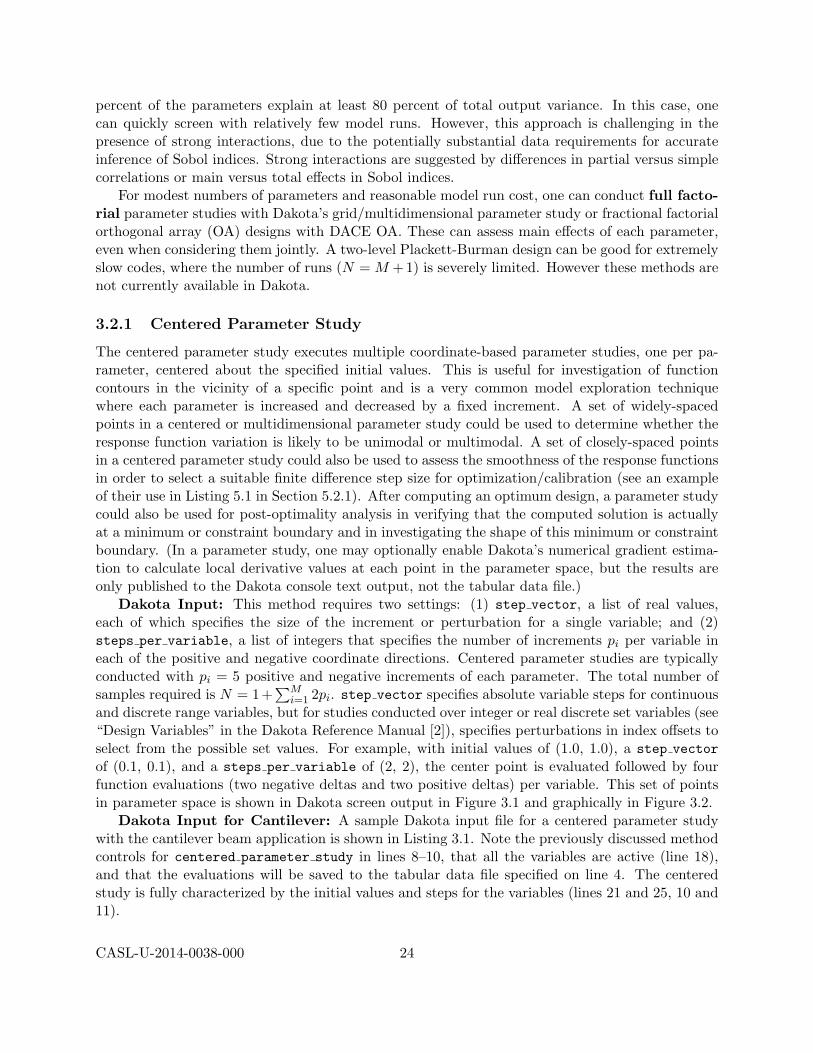
The centered parameter study executes multiple coordinate-based parameter studies, one per pa-rameter, centered about the specified initial values. This is useful for investigation of functioncontours in the vicinity of a specific point and is a very common model exploration techniquewhere each parameter is increased and decreased by a fixed increment. A set of widely-spacedpoints in a centered or multidimensional parameter study could be used to determine whether theresponse function variation is likely to be unimodal or multimodal. A set of closely-spaced pointsin a centered parameter study could also be used to assess the smoothness of the response functionsin order to select a suitable finite difference step size for optimization/calibration (see an exampleof their use in Listing 5.1 in Section 5.2.1). After computing an optimum design, a parameter studycould also be used for post-optimality analysis in verifying that the computed solution is actuallyat a minimum or constraint boundary and in investigating the shape of this minimum or constraintboundary. (In a parameter study, one may optionally enable Dakota’s numerical gradient estima-tion to calculate local derivative values at each point in the parameter space, but the results areonly published to the Dakota console text output, not the tabular data file.)
Dakota Input: This method requires two settings: (1) step vector, a list of real values,each of which specifies the size of the increment or perturbation for a single variable; and (2)steps per variable, a list of integers that specifies the number of increments pi per variable ineach of the positive and negative coordinate directions. Centered parameter studies are typicallyconducted with pi = 5 positive and negative increments of each parameter. The total number ofsamples required is N = 1 +
∑Mi=1 2pi. step vector specifies absolute variable steps for continuous
and discrete range variables, but for studies conducted over integer or real discrete set variables (see“Design Variables” in the Dakota Reference Manual [2]), specifies perturbations in index offsets toselect from the possible set values. For example, with initial values of (1.0, 1.0), a step vectorof (0.1, 0.1), and a steps per variable of (2, 2), the center point is evaluated followed by fourfunction evaluations (two negative deltas and two positive deltas) per variable. This set of pointsin parameter space is shown in Dakota screen output in Figure 3.1 and graphically in Figure 3.2.
Dakota Input for Cantilever: A sample Dakota input file for a centered parameter studywith the cantilever beam application is shown in Listing 3.1. Note the previously discussed methodcontrols for centered parameter study in lines 8–10, that all the variables are active (line 18),and that the evaluations will be saved to the tabular data file specified on line 4. The centeredstudy is fully characterized by the initial values and steps for the variables (lines 21 and 25, 10 and11).
CASL-U-2014-0038-000 24

Parameters for function evaluation 1:1.0000000000e+00 d11.0000000000e+00 d2
Parameters for function evaluation 2:8.0000000000e-01 d11.0000000000e+00 d2
Parameters for function evaluation 3:9.0000000000e-01 d11.0000000000e+00 d2
Parameters for function evaluation 4:1.1000000000e+00 d11.0000000000e+00 d2
Parameters for function evaluation 5:1.2000000000e+00 d11.0000000000e+00 d2
Parameters for function evaluation 6:1.0000000000e+00 d18.0000000000e-01 d2
Parameters for function evaluation 7:1.0000000000e+00 d19.0000000000e-01 d2
Parameters for function evaluation 8:1.0000000000e+00 d11.1000000000e+00 d2
Parameters for function evaluation 9:1.0000000000e+00 d11.2000000000e+00 d2
Figure 3.1: Dakota output showing function evaluations for a centered parameter study with twopositive and two negative steps per variable.
Figure 3.2: Notional example of centered parameter study over two parameters d1 and d2.
CASL-U-2014-0038-000 25

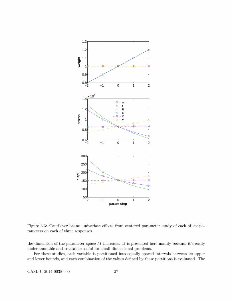
Results and Discussion: The results of the study are depicted in Figure 3.3, where thetabular data generated by Dakota (cantilever centered.dat) has been plotted with Matlab.These plots show that only w and t affect area /weight (the plots for these two variables overlayeach other). For the stress and displacement, w and t have the strongest effect, and possibly anonlinear one as evidence by the curvature in their traces. E and X have a small, but nonzeroeffect. All input/output relationships appear smooth (no noise or other oscillation is evident).These observations can be verified by studying the equations for the static cantilever problem.
Listing 3.1: Dakota input file showing centered parameter study on the cantilever beam problem.1 strategy ,
single_method
3 tabular_graphics_data
tabular_graphics_file ’cantilever_centered.dat ’
5
method ,
7
# do a parameter study in coordinate directions over all 6 parameters
9 centered_parameter_study
step_vector 0.1 0.1 10 100 10 100
11 steps_per_variable 2
13 variables ,
15 # by default , a parameter study won ’t operate on state parameters
# can change that default behavior be explicitly specifying which
17 # parameters to use (here "all")
active all
19
continuous_design = 2
21 initial_point 1.0 1.0
descriptors ’w’ ’t’
23
continuous_state = 4
25 initial_state 40000. 29.E+6 500. 1000.
descriptors ’R’ ’E’ ’X’ ’Y’
27
interface ,
29 direct
analysis_driver = ’mod_cantilever ’
31
responses ,
33 num_objective_functions = 3
response_descriptors = ’area ’ ’stress ’ ’displacement ’
35 no_gradients
no_hessians
3.2.2 Multidimensional Parameter Study
The multidimensional parameter study computes response data sets for an M -dimensional hyper-grid of input points. This full factorial design is powerful in determining main effects and potentialinteractions among parameters, but the number of simulation runs quickly becomes prohibitive as
CASL-U-2014-0038-000 26
−2 −1 0 1 20.8
0.9
1
1.1
1.2
1.3
wei
gh
t
−2 −1 0 1 20.6
0.8
1
1.2
1.4x 10
6
stre
ss
wtREXY
−2 −1 0 1 250
100
150
200
250
300
dis
pl
param step
Figure 3.3: Cantilever beam: univariate effects from centered parameter study of each of six pa-rameters on each of three responses.
the dimension of the parameter space M increases. It is presented here mainly because it’s easilyunderstandable and tractable/useful for small dimensional problems.
For these studies, each variable is partitioned into equally spaced intervals between its upperand lower bounds, and each combination of the values defined by these partitions is evaluated. The
CASL-U-2014-0038-000 27

number of function evaluations performed in the study is:
M∏i=1
(partitionsi + 1) (3.7)
Dakota Input Example: The partitions information is provided using the partitions speci-fication, which inputs an integer list of the number of partitions for each variable (i.e., partitionsi).Since the initial values will not be used, they need not be specified.
In a two variable example problem with d1 ∈ [0,2] and d2 ∈ [0,3] (as defined by the upperand lower bounds from the variables specification) and with partitions = (2,3), the interval [0,2]is divided into two equal-sized partitions and the interval [0,3] is divided into three equal-sizedpartitions. This two-dimensional grid, shown notionally in Figure 3.4, would result in the twelvefunction evaluations shown in Figure 3.5. See the first example in the Dakota User’s Manual [1]:Tutorial for additional notes to understand this study.
Figure 3.4: Example of multidimensional parameter study.
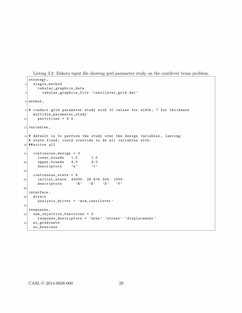
Dakota Input for Cantilever: Listing 3.2 shows a Dakota input file prescribing a multidi-mensional parameter study for the cantilever beam problem. On line 10, 9 partitions are specifiedfor w and 6 for t, resulting in 10× 7 = 70 total model evaluations in the (w, t) space. The parame-ters R,E,X, and Y are held at nominal values using Dakota’s state variable mechanism, as activeall is commented on line 16. In contrast to the centered parameter study, the active variables arecharacterized by their lower and upper bounds (lines 19–20).
Results and Discussion: When resources allow a grid parameter study to be conducted,one resulting advantage is that main effects can be calculated. An example is shown in Fig-ure 3.6. In this example, the main effects for w and t are generated by post-processing Dakota’scantilever grid.dat file using external statistical and plotting software. The left subplot showsthe main effect of w, that is the relationship between w and the mean of the displacement, takenover all realization of the other variable t. We observe a smooth, nonlinear effect. Similar is truefor the main effect of t in the right subplot.
CASL-U-2014-0038-000 28
Listing 3.2: Dakota input file showing grid parameter study on the cantilever beam problem.strategy ,
2 single_method
tabular_graphics_data
4 tabular_graphics_file ’cantilever_grid.dat ’
6 method ,
8 # conduct grid parameter study with 10 values for width , 7 for thickness
multidim_parameter_study
10 partitions = 9 6
12 variables ,
14 # default is to perform the study over the design variables , leaving
# state fixed; could override to do all variables with:
16 ## active all
18 continuous_design = 2
lower_bounds 1.0 1.0
20 upper_bounds 4.0 4.0
descriptors ’w’ ’t’
22
continuous_state = 4
24 initial_state 40000. 29.E+6 500. 1000.
descriptors ’R’ ’E’ ’X’ ’Y’
26
interface ,
28 direct
analysis_driver = ’mod_cantilever ’
30
responses ,
32 num_objective_functions = 3
response_descriptors = ’area ’ ’stress ’ ’displacement ’
34 no_gradients
no_hessians
CASL-U-2014-0038-000 29

Parameters for function evaluation 1:0.0000000000e+00 d10.0000000000e+00 d2
Parameters for function evaluation 2:1.0000000000e+00 d10.0000000000e+00 d2
Parameters for function evaluation 3:2.0000000000e+00 d10.0000000000e+00 d2
Parameters for function evaluation 4:0.0000000000e+00 d11.0000000000e+00 d2
Parameters for function evaluation 5:1.0000000000e+00 d11.0000000000e+00 d2
Parameters for function evaluation 6:2.0000000000e+00 d11.0000000000e+00 d2
Parameters for function evaluation 7:0.0000000000e+00 d12.0000000000e+00 d2
Parameters for function evaluation 8:1.0000000000e+00 d12.0000000000e+00 d2
Parameters for function evaluation 9:2.0000000000e+00 d12.0000000000e+00 d2
Parameters for function evaluation 10:0.0000000000e+00 d13.0000000000e+00 d2
Parameters for function evaluation 11:1.0000000000e+00 d13.0000000000e+00 d2
Parameters for function evaluation 12:2.0000000000e+00 d13.0000000000e+00 d2
Figure 3.5: Dakota output function evaluations for a grid parameter study, the tensor product ofthree steps in d1 with four steps in d2.
The plot shown here was generated using Minitab statistical software, but SAS (http://www.sas.com), JMP (www.jmp.com), R (http://www.r-project.org), Minitab (http://www.minitab.com), Matlab (http://www.mathworks.com/products/matlab), and other tools can produce sim-ilar graphics. Therefore we recommend CASL analysts use the tools present in the computingenvironment at their institution. Grid parameter studies also output correlation coefficients, dis-cussed at greater length in the next section.
CASL-U-2014-0038-000 30
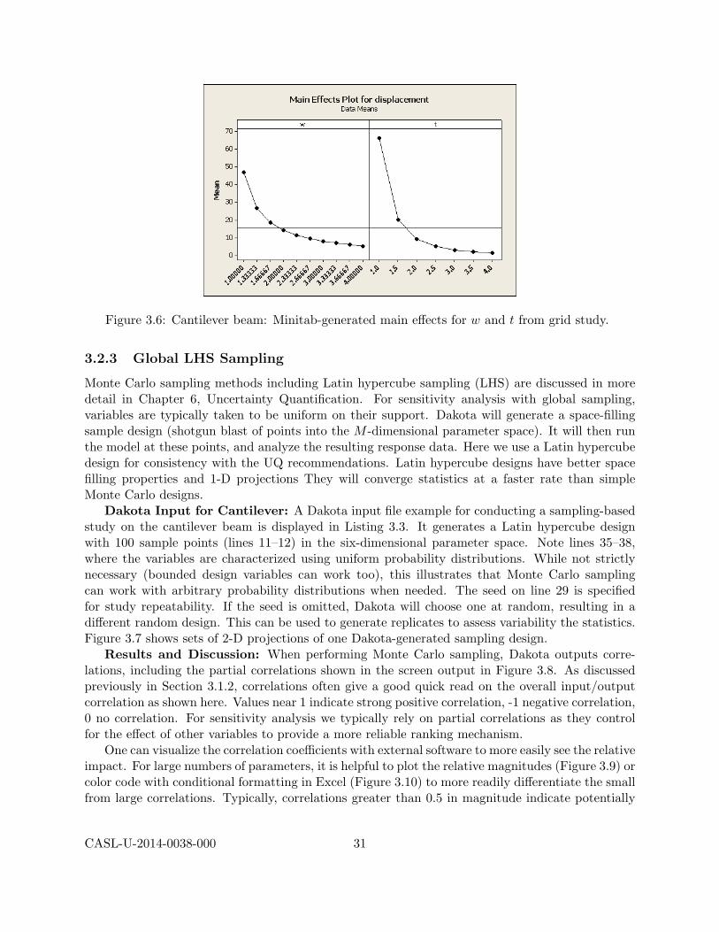
Figure 3.6: Cantilever beam: Minitab-generated main effects for w and t from grid study.
3.2.3 Global LHS Sampling
Monte Carlo sampling methods including Latin hypercube sampling (LHS) are discussed in moredetail in Chapter 6, Uncertainty Quantification. For sensitivity analysis with global sampling,variables are typically taken to be uniform on their support. Dakota will generate a space-fillingsample design (shotgun blast of points into the M -dimensional parameter space). It will then runthe model at these points, and analyze the resulting response data. Here we use a Latin hypercubedesign for consistency with the UQ recommendations. Latin hypercube designs have better spacefilling properties and 1-D projections They will converge statistics at a faster rate than simpleMonte Carlo designs.
Dakota Input for Cantilever: A Dakota input file example for conducting a sampling-basedstudy on the cantilever beam is displayed in Listing 3.3. It generates a Latin hypercube designwith 100 sample points (lines 11–12) in the six-dimensional parameter space. Note lines 35–38,where the variables are characterized using uniform probability distributions. While not strictlynecessary (bounded design variables can work too), this illustrates that Monte Carlo samplingcan work with arbitrary probability distributions when needed. The seed on line 29 is specifiedfor study repeatability. If the seed is omitted, Dakota will choose one at random, resulting in adifferent random design. This can be used to generate replicates to assess variability the statistics.Figure 3.7 shows sets of 2-D projections of one Dakota-generated sampling design.
Results and Discussion: When performing Monte Carlo sampling, Dakota outputs corre-lations, including the partial correlations shown in the screen output in Figure 3.8. As discussedpreviously in Section 3.1.2, correlations often give a good quick read on the overall input/outputcorrelation as shown here. Values near 1 indicate strong positive correlation, -1 negative correlation,0 no correlation. For sensitivity analysis we typically rely on partial correlations as they controlfor the effect of other variables to provide a more reliable ranking mechanism.
One can visualize the correlation coefficients with external software to more easily see the relativeimpact. For large numbers of parameters, it is helpful to plot the relative magnitudes (Figure 3.9) orcolor code with conditional formatting in Excel (Figure 3.10) to more readily differentiate the smallfrom large correlations. Typically, correlations greater than 0.5 in magnitude indicate potentially
CASL-U-2014-0038-000 31

Listing 3.3: Dakota input file showing global sampling on the cantilever beam problem.1 strategy ,
single_method
3 tabular_graphics_data
tabular_graphics_file ’cantilever_sa.dat ’
5
method ,
7
# do a sampling -based sensitivity study , optionally with
9 # variance -based decomposition to get higher order sensitivities
sampling
11 sample_type lhs
samples = 100
13 # variance_based_decomp
15 # do a design -of -experiments -based sensitivity using ANOVA to compute
# the sensitivities
17 # dace oas
# main_effects
19 # samples = 100
21 # do a Morris One -At -A-Time sensitivity study
# psuade_moat
23 # must be odd
# partitions = 3
25 # must be integer multiple of (num_vars + 1)
# samples = 98
27
# need these for all methods; seed allows for repeatability
29 seed = 52983
31 variables ,
33 # By default DACE and Sampling methods sample over all variables
35 uniform_uncertain = 6
upper_bounds 48000. 45.E+6 700. 1200. 2.2 2.2
37 lower_bounds 32000. 15.E+6 300. 800. 2.0 2.0
descriptors ’R’ ’E’ ’X’ ’Y’ ’w’ ’t’
39
interface ,
41 direct
analysis_driver = ’mod_cantilever ’
43
responses ,
45 num_response_functions = 3
response_descriptors = ’weight ’ ’stress ’ ’displ ’
47 no_gradients
no_hessians
CASL-U-2014-0038-000 32

2 2.1 2.2t
2 2.1 2.2w
800 1000 1200Y
400 600X
2 3 4
x 107E
3.5 4 4.5
x 104
2
2.1
2.2
R
t
2
2.1
2.2
w
800
1000
1200
Y
300
400
500
600
700X
2
3
4
x 107
E
3.5
4
4.5
x 104
R
Figure 3.7: Latin hypercube design example: 2-D projections showing locations in the parameterspace of 100 Monte Carlo samples using uniform distributions for all six parameters.
Partial Correlation Matrix between input and output:weight stress displ
R 1.36556e-01 -9.89955e-01 -5.82547e-02E -2.59807e-02 1.51530e-02 -9.53598e-01X -8.58158e-03 9.96167e-01 3.12725e-01Y 5.15226e-02 9.96214e-01 7.35493e-01w 9.99659e-01 -9.84197e-01 -4.20681e-01t 9.99659e-01 -9.89246e-01 -5.24940e-01
Figure 3.8: Dakota output showing partial correlations for the cantilever beam problem.
significant input/output relationships (though specific guidance and interpretation depends on thenumber of samples, number of variables, and analysis tolerance). Values less than 0.5 should bemore carefully studied for possible confounding factors or nonlinearities before discounting theirimportance.
As correlation coefficients are a linear measure of input/output relationship, it is critical tovisualize scatter plots to check for nonlinear trends. Figure 3.11 shows scatter plots generatedin Matlab, together with linear regression fits to the data. Some of the scatter plots exhibitnonlinear input/output trends in the cloud of data, for example the plots of E versus displ shows
CASL-U-2014-0038-000 33

−1 −0.5 0 0.5 1
REXYwt
Partial correlation for displ
Figure 3.9: Cantilever beam: partial correlation between displacement and inputs.
Partial Correlations for Cantilever
weight stress displ
R 0.14 -0.99 -0.06
E -0.03 0.02 -0.95
X -0.01 1.00 0.31
Y 0.05 1.00 0.74
w 1.00 -0.98 -0.42
t 1.00 -0.99 -0.52
Figure 3.10: Cantilever beam: partial correlation between displacement and inputs, conditionallyformatted with Microsoft Excel.
some curvature. Overall, however, the correlations are a good representative indicator of the mostimportant factors for these sample data.
Monte Carlo / LHS sampling for sensitivity analysis screening is typically conducted withnumber of samples equal to 10 times the number of variables, but budgets often push this downto a factor of two. Also, global Gaussian process models built in Dakota are typically constructedbased on a Latin hypercube design. Guidance on the number of samples for constructing suchsurrogates is provided in Chapter 4.
3.2.4 PSUADE/Morris Method
The Morris One-At-a-Time method, originally proposed by M. D. Morris [25], is a screening method,designed to explore a computational model to distinguish between input variables that have negligi-ble, linear and additive, or nonlinear/interaction effects on the output. The computer experimentsperformed consist of individually randomized designs which vary one input factor at a time to cre-ate a sample of its elementary effects. A more extensive discussion of the method and its metricscan be found in the “Design of Experiments Capabilities” chapter of the Dakota User’s Manual [1].
The file examples/SensitivityAnalysis/cantilever morris.in shows an alternate Dakota
CASL-U-2014-0038-000 34
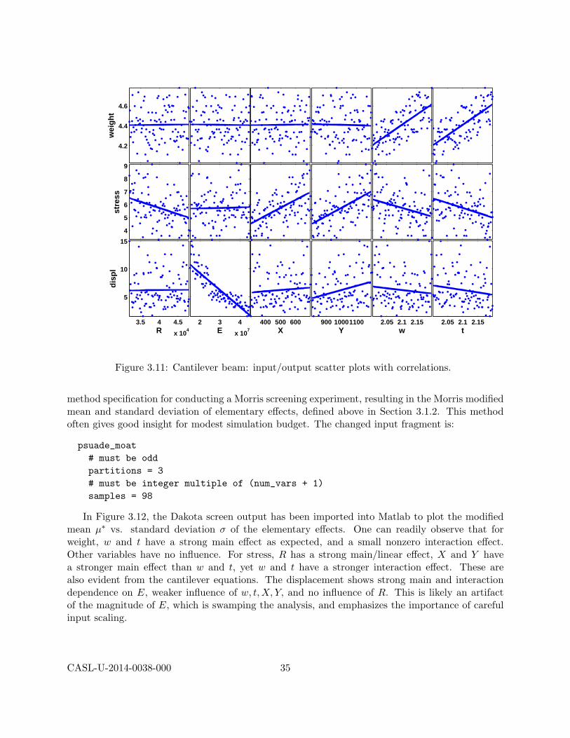
2.05 2.1 2.15t
2.05 2.1 2.15w
900 10001100Y
400 500 600X
2 3 4
x 107E
3.5 4 4.5
x 104
5
10
15
R
dis
pl
4
5
6
7
8
9x 10
4
stre
ss
4.2
4.4
4.6w
eig
ht
Figure 3.11: Cantilever beam: input/output scatter plots with correlations.
method specification for conducting a Morris screening experiment, resulting in the Morris modifiedmean and standard deviation of elementary effects, defined above in Section 3.1.2. This methodoften gives good insight for modest simulation budget. The changed input fragment is:
psuade_moat# must be oddpartitions = 3# must be integer multiple of (num_vars + 1)samples = 98
In Figure 3.12, the Dakota screen output has been imported into Matlab to plot the modifiedmean µ∗ vs. standard deviation σ of the elementary effects. One can readily observe that forweight, w and t have a strong main effect as expected, and a small nonzero interaction effect.Other variables have no influence. For stress, R has a strong main/linear effect, X and Y havea stronger main effect than w and t, yet w and t have a stronger interaction effect. These arealso evident from the cantilever equations. The displacement shows strong main and interactiondependence on E, weaker influence of w, t,X, Y, and no influence of R. This is likely an artifactof the magnitude of E, which is swamping the analysis, and emphasizes the importance of carefulinput scaling.
CASL-U-2014-0038-000 35
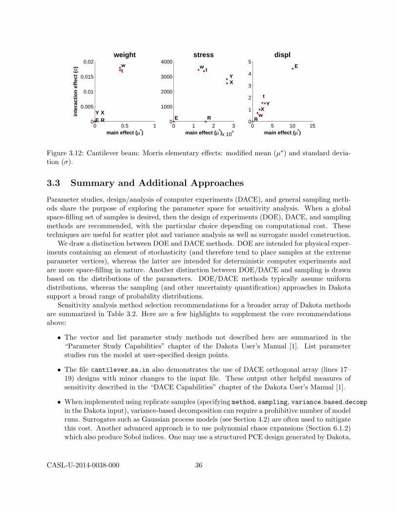
0 0.5 10
0.005
0.01
0.015
0.02
main effect (µ*)
inte
ract
ion
eff
ect
(σ)
REXY
wt
weight
0 1 2 3
x 104
0
1000
2000
3000
4000
main effect (µ*)
RE
XY
w t
stress
0 5 10 150
1
2
3
4
5
main effect (µ*)
R
E
XY
w
t
displ
Figure 3.12: Cantilever beam: Morris elementary effects: modified mean (µ∗) and standard devia-tion (σ).
3.3 Summary and Additional Approaches
Parameter studies, design/analysis of computer experiments (DACE), and general sampling meth-ods share the purpose of exploring the parameter space for sensitivity analysis. When a globalspace-filling set of samples is desired, then the design of experiments (DOE), DACE, and samplingmethods are recommended, with the particular choice depending on computational cost. Thesetechniques are useful for scatter plot and variance analysis as well as surrogate model construction.
We draw a distinction between DOE and DACE methods. DOE are intended for physical exper-iments containing an element of stochasticity (and therefore tend to place samples at the extremeparameter vertices), whereas the latter are intended for deterministic computer experiments andare more space-filling in nature. Another distinction between DOE/DACE and sampling is drawnbased on the distributions of the parameters. DOE/DACE methods typically assume uniformdistributions, whereas the sampling (and other uncertainty quantification) approaches in Dakotasupport a broad range of probability distributions.
Sensitivity analysis method selection recommendations for a broader array of Dakota methodsare summarized in Table 3.2. Here are a few highlights to supplement the core recommendationsabove:
• The vector and list parameter study methods not described here are summarized in the“Parameter Study Capabilities” chapter of the Dakota User’s Manual [1]. List parameterstudies run the model at user-specified design points.
• The file cantilever sa.in also demonstrates the use of DACE orthogonal array (lines 17–19) designs with minor changes to the input file. These output other helpful measures ofsensitivity described in the “DACE Capabilities” chapter of the Dakota User’s Manual [1].
• When implemented using replicate samples (specifying method, sampling, variance based decompin the Dakota input), variance-based decomposition can require a prohibitive number of modelruns. Surrogates such as Gaussian process models (see Section 4.2) are often used to mitigatethis cost. Another advanced approach is to use polynomial chaos expansions (Section 6.1.2)which also produce Sobol indices. One may use a structured PCE design generated by Dakota,
CASL-U-2014-0038-000 36

or import the points from a previous Monte Carlo sample to build the PCE and quickly cal-culate the variance-based decomposition.
• Other design types may be more appropriate for polynomial regression such as Box-Behnken [7]or central composite design [8] for quadratic polynomials.
Table 3.2: Guidelines for selection of parameter study, DOE, DACE, and sampling methods.
Method Applications Applicable MethodsClassification
parameter study sensitivity analysis, centered parameter study,directed parameter space list parameter study,
investigations multidim parameter study,vector parameter study
classical design physical experiments dace (box behnken,of experiments (parameters uniformly distributed) central composite)
design of variance analysis, dace (grid, random, oas, lhs, oa lhs),computer space filling designs fsu quasi mc (halton, hammersley),
experiments (parameters uniformly distributed) fsu cvt, psuade moat
sampling space filling designs sampling (Monte Carlo, LHS)(parameters have with optional
general probability distributions) active view override
CASL-U-2014-0038-000 37

Chapter 4
Surrogate Models
This chapter introduces the basic theory and use of Dakota’s polynomial regression and krigingsurrogate models. Surrogate models are typically employed to provide computationally efficientapproximate representations of trends and residual (error) processes in physical data or code output.The terms “emulator,” “response surface,” and “meta-model” refer to the generation of surrogatepredictions with associated uncertainty quantification. In the Dakota context, surrogate models areautomatically generated based on empirical samples of the true simulation model’s input/outputrelationship. This type of surrogate can be constrasted with physics-based surrogates which makesimplifying assumptions to create a simpler, faster running simulation model.
In the following, Y (x) denotes a surrogate for the physical or computational response of in-terest f(x), µ(x) denotes the prediction of Y (x) evaluated at the input x (emulator mean), andσ(x) denotes the standard error of prediction evaluated at the input x (emulator standard error).Emulators are constructed from physical data or code output collected on a sample design of Nruns in M input dimensions. Good practice requires the run size N to be at least as large as thenumber of surrogate model parameters requiring estimation (degrees of freedom). Dakota enforcesthis practice by exiting and returning an error message if N is too small. The degrees of freedom(and thus minimum N) will be stated for each surrogate model introduced in the ensuing sections.
The surrogate models considered in this chapter assume the distribution of residuals (differencebetween experimental or code output and emulator prediction) is modeled as mean-zero Gaussian.Diagnostics such as a normal probability plot of standardized emulator residuals can be used tocheck this assumption, as illustrated in Section 7.3.2. Under the assumption of Gaussian residuals,outputs used to construct emulators will then follow a multivariate Gaussian distribution, assumingall unknown surrogate model parameters are fixed. The likelihood of observing the given outputsfor any given value of the surrogate model parameters is the associated value of this multivariateGaussian density function. In this chapter, most surrogate model parameters are estimated bymaximum likelihood in Dakota, by finding a value for these parameters that maximizes the likeli-hood function. This value is referred to as the maximum likelihood estimate (MLE). Parameterestimation via MLE differs from the Bayesian approach to parameter inference discussed in Un-certainty Quantification, Chapter 6, in that the latter results in a probability distribution for thesurrogate model parameters. In practice, the contribution to overall emulator uncertainty inducedby surrogate model parameter uncertainty from Bayesian inference is often small compared withthe uncertainty arising from the residual error process itself. Computations in Dakota involvingsurrogate model indirection can thus be sped up considerably by utilizing a point estimate (the
CASL-U-2014-0038-000 38

MLE) in place of a probability distribution for the surrogate model parameters.Section 4.1 considers polynomial surrogates, which are typically used to model observed trends
in data from physical experiments resulting from perturbing input parameters that describe physicalscenarios of interest. Polynomial surrogates model these trends as a regression relationship thatis linear in the unknown coefficients (but not necessarily in the inputs themselves). Experimentalerrors are assumed to be independently distributed as mean-zero Gaussian distributions havingcommon variance. Polynomial surrogates smooth the observed data by finding the best-fittingtrend model of those in the class specified by the user.
Section 4.2 considers kriging surrogates, which are typically used to model observed trends inoutputs from computationally intensive code runs resulting from input parameter perturbations.In this setting, input parameters describe physical scenarios of interest as well as uncertain ini-tial or boundary conditions, or possibly uncertain closure model parameters that are calibrated toexperimental data (see Optimization and Deterministic Calibration, Chapter 5 and UncertaintyQuantification, Chapter 6). Assuming the quantities of interest vary smoothly with input pertur-bations, the information available from a small number of code runs can be used effectively bythe kriging surrogate to infer a correlated error structure. The kriging surrogate is thus able toborrow strength from the small set of code runs conducted to quickly predict code output at userspecified input settings with quantified uncertainty. Code runs “closer” to a desired predictionsite are weighted more heavily in constructing the kriging emulator than those further away withrespect to the inferred correlation structure.
Typically, kriging surrogates interpolate the set of code runs made for the purpose of inferring thesurrogate model parameters. That is, emulator predictions at input sites corresponding to availablecode runs are equal to the calculated code outputs with zero uncertainty. This interpolationproperty is often desirable for emulating deterministic codes that produce a single output valueover repeated runs at the same input point. However, as described in Section 4.2 it is possible torelax this interpolation property when fitting a kriging model. This option is useful for leveragingthe flexibility of kriging surrogates to model data from physical experiments (e.g. if polynomialsurrogates do not provide an adequate fit), or to model output from stochastic codes or deterministiccodes subject to numerical or high frequency noise.
As described in the ensuing sections, diagnostics are available to assess the predictive capabilityof a chosen surrogate model. We synthesize the discussion above to make the following recommen-dations on the initial choice of surrogate model. Polynomial surrogates are often employed to modeloutputs from physical experiments. Polynomial or kriging surrogates may be utilized to model codeoutput. Polynomial surrogates are appropriate when very few input parameters are being variedor prior knowledge indicates the trend contains minimal contribution from input nonlinearity andinteraction. Subject to these considerations regarding trend complexity, polynomial surrogates areparticularly appropriate for modeling stochastic or noisy code outputs. Kriging surrogates areideal for settings in which weak or nonexistant prior information exists about trend complexity.They are often able to successfully infer the trend from a modest set of training runs, yielding anadvantage over the effort often required to successfully fit a suitable polynomial surrogate in thepresence of little or no prior information about trends. Kriging surrogates are also capable of fit-ting nonlinear trends not easily represented by low order polynomial surrogates. For deterministiccodes, the uncertainty quantification provided by kriging surrogates conforms to the notion thatprediction uncertainty should diminish near input points at which training runs were conducted.This behavior does not occur with polynomial surrogates.
CASL-U-2014-0038-000 39

4.1 Polynomial Regression Models
Linear, quadratic, and cubic polynomial surrogate models are available in Dakota. The form of thelinear polynomial model is
Y (x) = β0 +M∑i=1
βixi + ε(x) ;
the form of the quadratic polynomial model is
Y (x) = β0 +M∑i=1
βixi +M∑i=1
M∑j≥i
βijxixj + ε(x) ;
and the form of the cubic polynomial model is
Y (x) = β0 +M∑i=1
βixi +M∑i=1
M∑j≥i
βijxixj +M∑i=1
M∑j≥i
M∑k≥j
βijkxixjxk + ε(x) .
In all of the polynomial models, Y (x) is the response of the polynomial model plus a mean-zeroGaussian error model (ε(x)); the xi, xj , xk terms are the components of the M -dimensional inputparameter values; and the β0, βi, βij , and βijk terms are the polynomial coefficients. The numberof coefficients, Nβ, depends on the order of the polynomial model. For the linear polynomial,Nβ = M + 1; for the quadratic polynomial, Nβ = (M + 1)(M + 2)/2; and for the cubic polynomial,Nβ = (M3 + 6M2 + 11M + 6)/6. The errors ε(·) associated with each output are assumed to beindependently distributed and have constant variance σ2.
There must be at least Nβ data samples (i.e. N ≥ Nβ) in order to form a fully determinedlinear system and solve for the polynomial coefficients β. In most applications, the linear systemwill be overdetermined (i.e. N > Nβ). To solve such systems, Dakota employs a least-squaresapproach involving a QR factorization-based numerical method. Note that N ≥ Nβ + 1 is requiredto estimate both β and the error variance σ2.
The maximum likelihood value of β is computed via ordinary least squares,
β =(GTG
)−1GT y .
Here y is the N -vector of observed experimental data and G is a N by Nβ matrix that containsevaluations of the polynomial basis functions at all runs in the N by M sample design X, Gij =gj(XTi
), i = 1, . . . , N ; j = 1, . . . , Nβ.
The emulator mean µ(x) evaluated at input x is a best linear unbiased predictor of the surrogateY (x),
µ(x) = gT (x)β .
The emulator variance σ2(x) (here, the mean squared error of prediction) evaluated at input xprovides a spatially varying measure of prediction uncertainty,
σ2(x) = σ2(
1 + gT (x)(GTG
)−1g(x)
),
where an unbiased estimate of σ2 is
σ2 =
(y −Gβ
)T (y −Gβ
)N −Nβ
.
CASL-U-2014-0038-000 40

The utility of the polynomial models stems from two sources: (1) over a small portion of theparameter space, a low-order polynomial model is often an accurate approximation to the truedata trends, and (2) the least-squares procedure provides a surface fit that smooths out noise inthe data. For this reason, surrogate-based optimization is often successful when using polynomialmodels, particularly quadratic models. However, a polynomial surface fit may not be the bestchoice for modeling data trends over the entire parameter space, unless it is known a priori that thetrue data trends are close to linear, quadratic, or cubic. Furthermore, in general polynomial modelswill not interpolate, i.e. predict with zero uncertainty, the data they are built from. If interpolationis desired (as with deterministic computational models subject to negligible numerical noise), or iflack of fit is observed, users should consider the kriging emulators described in the following section.See [27] for additional information on polynomial models.
4.1.1 Fitting Polynomial Surrogates in Dakota
In the following discussion, typewriter font indicates the names of Dakota input or output files,keywords, commands, or results. All input, output, and log files mentioned in this subsectioncan be found in examples/SurrogateModels. Listings 4.1 and 4.2 together show the Dakotainput file cantilever polynomial eval.in for evaluating a quadratic polynomial emulator of thecantilever beam model outputs at user-specified values of the inputs x. The values of x at which toevaluate the emulator are given in the list parameter study block of the input file (line 22). Thekeyword sampling (line 58), together with sample type lhs (line 60) tells Dakota to generate aLatin hypercube sample. Dakota then runs the cantilever beam model on the resulting 60 inputsettings (line 61), producing output for the three indicated response variables (area, stress, anddisplacement). The design and output results are then used by Dakota to fit a quadratic polynomialmodel to each response (line 37). Dakota also allows linear and cubic polynomial trend options.Finally, predicted responses corresponding to each user specified input setting are written to thefile cantilever polynomial evals.dat (line 9):
%eval_id R E X Y w t area stress displacement1 32887.97269 36889581.78 408.9821034 1148.6638 2.099541047 2.004037063 4.207558073 76546.06547 5.9142534882 43482.92921 16550393.66 639.6736606 1051.841799 2.014840025 2.19097364 4.414461384 64938.20937 11.961421273 36220.72048 44845837.48 561.1743862 935.4138043 2.109386061 2.136922015 4.507593512 57481.41311 2.6277952264 47325.31136 25228026.72 348.841119 876.590786 2.190414084 2.082472944 4.561478066 28938.90198 5.259963951
By specifying a random number seed (line 59), the results obtained from running Dakota arerepeatable, which is useful for regression testing purposes and for situations in which intermediateresults (such as experimental designs) must be regenerated exactly in follow-on Dakota analyses.
In this example, we chose to generate a Latin hypercube sample to fit the quadratic surrogatemodel. Latin hypercube samples are frequently used to fit kriging surrogates (Section 4.2) forcomplex computational model quantities of interest due to their space-filling nature; however,they can be less efficient than various alternatives more commonly selected for fitting polynomialsurrogates, particularly when modeling responses from physical experiments subject to observationerror. Two such alternatives for obtaining quadratic emulators are available in Dakota, selectedby replacing the sampling block with dace central composite for central composite designs [8]or dace box behnken for Box-Behnken designs [7]. Central composite designs generate N = 1 +2M+2M samples, while Box-Behnken designs generate N = 1+4M(M−1)/2 samples. A seed canalso be specified with dace options for repeatability. The option dace oas allows for generation
CASL-U-2014-0038-000 41
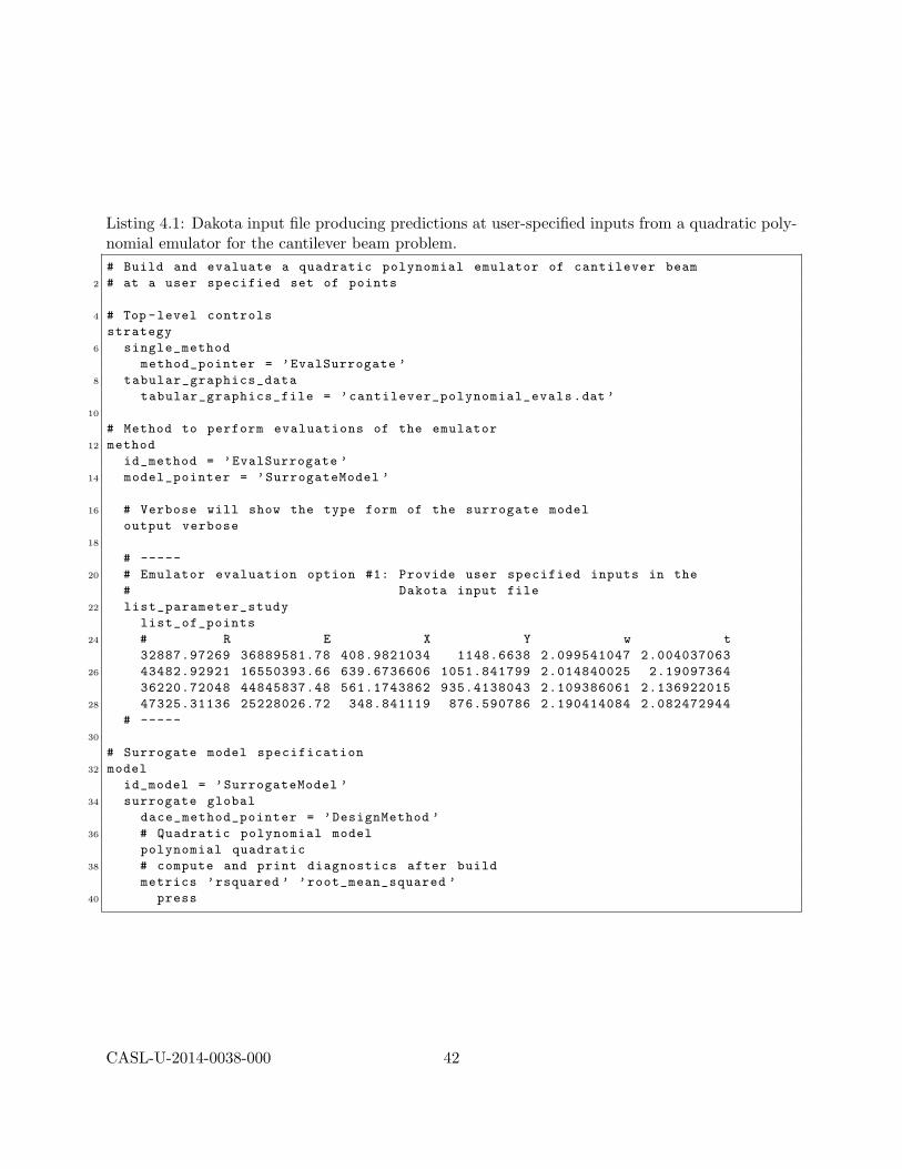
Listing 4.1: Dakota input file producing predictions at user-specified inputs from a quadratic poly-nomial emulator for the cantilever beam problem.# Build and evaluate a quadratic polynomial emulator of cantilever beam
2 # at a user specified set of points
4 # Top -level controls
strategy
6 single_method
method_pointer = ’EvalSurrogate ’
8 tabular_graphics_data
tabular_graphics_file = ’cantilever_polynomial_evals.dat ’
10
# Method to perform evaluations of the emulator
12 method
id_method = ’EvalSurrogate ’
14 model_pointer = ’SurrogateModel ’
16 # Verbose will show the type form of the surrogate model
output verbose
18
# -----
20 # Emulator evaluation option #1: Provide user specified inputs in the
# Dakota input file
22 list_parameter_study
list_of_points
24 # R E X Y w t
32887.97269 36889581.78 408.9821034 1148.6638 2.099541047 2.004037063
26 43482.92921 16550393.66 639.6736606 1051.841799 2.014840025 2.19097364
36220.72048 44845837.48 561.1743862 935.4138043 2.109386061 2.136922015
28 47325.31136 25228026.72 348.841119 876.590786 2.190414084 2.082472944
# -----
30
# Surrogate model specification
32 model
id_model = ’SurrogateModel ’
34 surrogate global
dace_method_pointer = ’DesignMethod ’
36 # Quadratic polynomial model
polynomial quadratic
38 # compute and print diagnostics after build
metrics ’rsquared ’ ’root_mean_squared ’
40 press
CASL-U-2014-0038-000 42

Listing 4.2: (Continued) Dakota input file producing predictions at user-specified inputs from aquadratic polynomial emulator for the cantilever beam problem.
42 variables ,
uniform_uncertain = 6
44 upper_bounds 48000. 45.E+6 700. 1200. 2.2 2.2
lower_bounds 32000. 15.E+6 300. 800. 2.0 2.0
46 descriptors ’R’ ’E’ ’X’ ’Y’ ’w’ ’t’
48 responses
response_functions = 3
50 descriptors = ’area ’ ’stress ’ ’displacement ’
no_gradients
52 no_hessians
54 # Method to generate a 60 run Latin hypercube design to build the emulator
method
56 id_method = ’DesignMethod ’
model_pointer = ’SimulationModel ’
58 sampling
seed = 20
60 sample_type lhs
samples = 60
62
# The true simulation model to evaluate to build the emulator
64 model
id_model = ’SimulationModel ’
66 single
interface_pointer = ’SimulationInterface ’
68
interface ,
70 id_interface = ’SimulationInterface ’
direct
72 analysis_driver = ’mod_cantilever ’
CASL-U-2014-0038-000 43

of orthogonal array designs [18] to support polynomial surrogate fits and main effects analysis(Chapter 3).
Dakota was run with the command dakota -i cantilever polynomial eval.in >& reg.log
&. The log file reg.log provides the surrogate parameter estimates β and σ2, as well as leave-one-out cross-validation root mean squared prediction errors (input file, line 40) for each output, whichevaluated to 8.3476172226e-16, 5.2744083954e+01, and 3.7407615270e-01 for area, stress, anddisplacement respectively. The root mean squared prediction error (RMSPE) provides a goodoverall estimate of emulator out-of-sample predictive capability.
A K-fold cross-validation procedure is also available in Dakota by replacing the press option(line 40) with cross validate folds = K. The K-fold cross-validation procedure involves ran-domly partitioning the training data into K subsets, each containing approximately 100/K% ofthe data. For each subset, the 100/K% of the design runs and their corresponding outputs are “heldout”, and the surrogate refitted with the remaining 100 ∗ (K − 1)/K% of the design runs and asso-ciated outputs. The 100/K% hold-out points are then predicted by the refitted emulator. Thus atotal of K surrogate rebuilds are conducted, each leaving out 100/K% of the original training data,and the RMSPE is computed for all of the hold-out design points over the whole procedure. Run-ning Dakota with K = 10, the RMSPE evaluated to 6.1748098826e-16, 5.3512924399e+01, and3.8966016172e-01 for area, stress, and displacement respectively. These results are qualitativelysimilar to the leave-one-out cross-validation results. Note that the leave-one-out cross-validationprocedure is equivalent to N -fold cross-validation.
4.2 Kriging and Gaussian Process Models
The set of techniques known as kriging were originally developed in the geostatistics and spatialstatistics communities to produce maps of underground geologic deposits based on a set of widelyand irregularly spaced borehole sites [9]. Building a kriging model typically involves the
1. Choice of a trend function,
2. Choice of a correlation function, and
3. Estimation of correlation parameters.
Suppose outputs (e.g. deposits from the borehole sites) are to be collected at the N inputs{x1, . . . , xN} to train a kriging surrogate Y (x) for the output at input x. The emulator used for pre-diction of Y (x) is assumed to be linear in these outputs, Y (x) =
∑Ni=1 ci(x)Y (xi). The coefficient
vector c(x) is determined by minimizing the mean squared error of prediction E[(Y (x)− Y (x)
)2]
for fixed correlation parameters, subject to the unbiasedness constraint E[Y (x)
]= E [Y (x) ]. The
notation E[ · ] indicates expected value. The optimized mean squared error of prediction quantifiesthe uncertainty in prediction of Y (x).
Kriging surrogates can also be derived from Gaussian processes, which further assume thatarbitrary collections of observed outputs follow multivariate Gaussian distributions for fixed trend,variance and correlation parameters. In Dakota, the Gaussian process (GP) framework is adoptedto facilitate covariance parameter estimation through techniques such as maximum likelihood anduncertainty quantification via standard statistical inference methods.
CASL-U-2014-0038-000 44

A kriging surrogate, Y (x), consists of a trend function (frequently a linear model gT (x)β) plusa Gaussian process error model (ε(x)) that modifies the trend function locally,
Y (x) = gT (x)β + ε(x) .
This specifies a stochastic process representation of the unknown true surface f(x). The errorprocess ε(x) is assumed initially to have mean zero and constant variance σ2. Furthermore, corre-lated errors in the input space are allowed by specifying a covariance function. In particular, thecovariance between the errors at two arbitrary input locations x and x′ is modeled as
Cov(Y (x), Y (x′)
)= Cov
(ε(x), ε(x′)
)= σ2 r
(x, x′
),
where r (x, x′) is a correlation function (i.e. a symmetric, positive definite function satisfyingr (x, x) = 1). In the following, this correlation function is assumed to depend on the values ofunknown parameters φ, designated r (x, x′|φ).
When the true surface results from evaluation of a deterministic computational model, theerror process ε(x) can be specified in such a way that the emulator will interpolate, with zerouncertainty, the model runs it was built from. This is accomplished through selection of a corre-lation function with requisite smoothness properties, discussed further below. The error processspecification is modified as follows to accommodate physical experiments subject to measurementor replicate variability, stochastic computational models, or deterministic computational models forwhich numerical or high frequency noise is of concern,
Cov(ε(x), ε(x′)
)= σ2 r
(x, x′|φ)+ ∆2δ
(x− x′) ,
where
δ(x− x′) =
{1 if x− x′ = 00 otherwise
and ∆2 is the variance of the observational or numerical error. In the ensuing discussion, the term“nugget” refers to the ratio η = ∆2/σ2.
Figure 4.1 illustrates the behavior of emulators that interpolate versus emulators that smoothoutput data. In each panel, the red filled circles represent observed outputs and the red curvedesignates the emulator mean. The gray shaded area outlines the ensemble of pointwise 95%prediction intervals as a function of the input x, computed using the emulator standard error. Thatis, for any specified x, there is 95% probability that a future sampled output would lie between thelower and upper bounds of the gray shaded area. The left panel illustrates an error process selectedfor interpolation. Note the emulator mean passes directly through the three observed outputs, andthere is no emulator uncertainty at these points (zero width to the prediction intervals). Predictionuncertainty grows as the input level x moves away from any input location at which output isobserved. The right panel illustrates an error process selected for smoothing. In this case, theemulator mean defines a smooth surface that predicts the four observed outputs without beingrequired to recover their values exactly with zero uncertainty. The prediction intervals do notnarrow as x approaches an input location at which output is observed. Kriging models with nonugget effect (η = 0) will interpolate, while polynomial models or kriging models with a positivenugget effect (η > 0) will smooth.
By convention, the terms simple kriging, ordinary kriging, and universal kriging are used toindicate the three most common choices for the trend function. In simple kriging, the trend is
CASL-U-2014-0038-000 45
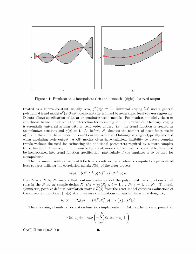
x
y ●●
●
x
y
●●
●
●
Figure 4.1: Emulator that interpolates (left) and smooths (right) observed output.
treated as a known constant, usually zero, gT (x)β ≡ 0. Universal kriging [24] uses a generalpolynomial trend model gT (x)β with coefficients determined by generalized least squares regression.Dakota allows specification of linear or quadratic trend models. For quadratic models, the usercan choose to include or omit the interaction terms among the input variables. Ordinary krigingis essentially universal kriging with a trend order of zero, i.e. the trend function is treated asan unknown constant and g(x) = 1. As before, Nβ denotes the number of basis functions ing(x) and therefore the number of elements in the vector β. Ordinary kriging is typically selectedwhen emulating code output, as GP models often have sufficient flexibility to detect complextrends without the need for estimating the additional parameters required by a more complextrend function. However, if prior knowledge about more complex trends is available, it shouldbe incorporated into trend function specification, particularly if the emulator is to be used forextrapolation.
The maximum likelihood value of β for fixed correlation parameters is computed via generalizedleast squares utilizing the correlation matrix R(φ) of the error process,
β(φ) =(GTR−1(φ)G
)−1GTR−1(φ) y .
Here G is a N by Nβ matrix that contains evaluations of the polynomial basis functions at allruns in the N by M sample design X, Gij = gj
(XTi
), i = 1, . . . , N ; j = 1, . . . , Nβ. The real,
symmetric, positive-definite correlation matrix R(φ) from the error model contains evaluations ofthe correlation function r(·, ·|φ) at all pairwise combinations of runs in the sample design X,
Rij(φ) = Rji(φ) = r(XTi , X
Tj |φ)
= r(XTj , X
Ti |φ)
There is a single family of correlation functions implemented in Dakota, the power exponential:
r (xi, xj |φ) = exp
(−
M∑k=1
φk |xik − xjk|γ)
CASL-U-2014-0038-000 46
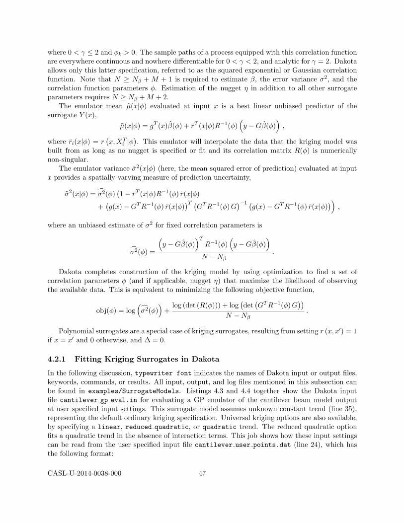
where 0 < γ ≤ 2 and φk > 0. The sample paths of a process equipped with this correlation functionare everywhere continuous and nowhere differentiable for 0 < γ < 2, and analytic for γ = 2. Dakotaallows only this latter specification, referred to as the squared exponential or Gaussian correlationfunction. Note that N ≥ Nβ + M + 1 is required to estimate β, the error variance σ2, and thecorrelation function parameters φ. Estimation of the nugget η in addition to all other surrogateparameters requires N ≥ Nβ +M + 2.
The emulator mean µ(x|φ) evaluated at input x is a best linear unbiased predictor of thesurrogate Y (x),
µ(x|φ) = gT (x)β(φ) + rT (x|φ)R−1(φ)(y −Gβ(φ)
),
where ri(x|φ) = r(x,XT
i |φ). This emulator will interpolate the data that the kriging model was
built from as long as no nugget is specified or fit and its correlation matrix R(φ) is numericallynon-singular.
The emulator variance σ2(x|φ) (here, the mean squared error of prediction) evaluated at inputx provides a spatially varying measure of prediction uncertainty,
σ2(x|φ) = σ2(φ)(1− rT (x|φ)R−1(φ) r(x|φ)
+(g(x)−GTR−1(φ) r(x|φ)
)T (GTR−1(φ)G
)−1 (g(x)−GTR−1(φ) r(x|φ)
)),
where an unbiased estimate of σ2 for fixed correlation parameters is
σ2(φ) =
(y −Gβ(φ)
)TR−1(φ)
(y −Gβ(φ)
)N −Nβ
.
Dakota completes construction of the kriging model by using optimization to find a set ofcorrelation parameters φ (and if applicable, nugget η) that maximize the likelihood of observingthe available data. This is equivalent to minimizing the following objective function,
obj(φ) = log(σ2(φ)
)+
log (det (R(φ))) + log(det(GTR−1(φ)G
))N −Nβ
.
Polynomial surrogates are a special case of kriging surrogates, resulting from setting r (x, x′) = 1if x = x′ and 0 otherwise, and ∆ = 0.
4.2.1 Fitting Kriging Surrogates in Dakota
In the following discussion, typewriter font indicates the names of Dakota input or output files,keywords, commands, or results. All input, output, and log files mentioned in this subsection canbe found in examples/SurrogateModels. Listings 4.3 and 4.4 together show the Dakota inputfile cantilever gp eval.in for evaluating a GP emulator of the cantilever beam model outputat user specified input settings. This surrogate model assumes unknown constant trend (line 35),representing the default ordinary kriging specification. Universal kriging options are also available,by specifying a linear, reduced quadratic, or quadratic trend. The reduced quadratic optionfits a quadratic trend in the absence of interaction terms. This job shows how these input settingscan be read from the user specified input file cantilever user points.dat (line 24), which hasthe following format:
CASL-U-2014-0038-000 47

%eval_id R E X Y w t1 32887.97269 36889581.78 408.9821034 1148.6638 2.099541047 2.0040370632 43482.92921 16550393.66 639.6736606 1051.841799 2.014840025 2.190973643 36220.72048 44845837.48 561.1743862 935.4138043 2.109386061 2.1369220154 47325.31136 25228026.72 348.841119 876.590786 2.190414084 2.082472944
The keyword sampling (line 56) together with sample type lhs (line 58) tells Dakota to generatea Latin hypercube sample. Dakota then runs the cantilever beam model on the resulting 60 inputsettings (line 59), producing output for the three indicated response variables (area, stress, anddisplacement). The design and output results are then used by Dakota to fit a GP with estimatedconstant trend to each response, and finally predicted responses corresponding to each user specifiedinput setting are written to the file cantilever gp evals.dat (line 9):
%eval_id R E X Y w t area stress displacement1 32887.97269 36889581.78 408.9821034 1148.6638 2.099541047 2.004037063 4.209402759 76378.17522 5.3609936942 43482.92921 16550393.66 639.6736606 1051.841799 2.014840025 2.19097364 4.413155956 65000.4832 12.419424513 36220.72048 44845837.48 561.1743862 935.4138043 2.109386061 2.136922015 4.506773804 57529.4144 2.5118575354 47325.31136 25228026.72 348.841119 876.590786 2.190414084 2.082472944 4.560423301 29135.16863 5.260298986
By specifying a random number seed (line 57), the results obtained from running Dakota arerepeatable.
A minimum run size was previously indicated based on the desire to obtain at least as manyruns as unknown surrogate parameters. However, more conservative run sizes are often selected,such as a factor of 10 times the number of “active inputs.” Since this latter quantity is often notknown, N = 10M is often selected [23]. With M = 6, this is the basis for the run size of 60 chosenfor this example.
Dakota was run with the command dakota -i cantilever gp eval.in >& gp.log &. Thelog file gp.log provides the surrogate parameter estimates φ, β(φ) and σ2(φ), as well as theleave-one-out cross-validation RMSPEs (input file, line 38) for each output, which evaluated to1.1264992653e-03, 1.4913388456e+02, and 1.1507679873e-01 for area, stress, and displace-ment respectively. For K = 10, the cross-validation RMSPEs for each output evaluated to1.2088124274e-03, 1.4905338700e+02, and 1.4178321830e-01 for area, stress, and displacementrespectively. Kriging fits can be adversely affected if the proportion of runs held out for cross-validation is too large (problem dependent), so it is typical to use K = N (i.e. leave-one-out) inthis setting.
Table 4.1 collects the four predictions of each output made by the quadratic polynomial andkriging emulators for comparison with direct code calculations. These predictions track variationin the code calculations well, an observation consistent with the small size of the cross-validationRMSPEs relative to the observed range in the calculations for each output.
4.3 Summary
Table 4.2 summarizes the essential Dakota options for specifying polynomial regression or krigingmodels, with guidance on which method is to be preferred based on the nature of the physical/-computational experiment output and assumptions about the statistical modeling of residual error.Additional details on fitting kriging and other surrogates such as multivariate adaptive regression
CASL-U-2014-0038-000 48

Listing 4.3: Dakota input file producing predictions at user specified inputs from a GP emulatorwith estimated constant trend for the cantilever beam problem.# Build and evaluate a Gaussian process emulator of cantilever beam
2 # at a user specified set of points
4 # Top -level controls
strategy
6 single_method
method_pointer = ’EvalSurrogate ’
8 tabular_graphics_data
tabular_graphics_file = ’cantilever_gp_evals.dat ’
10
12 # Method to perform evaluations of the emulator
method
14 id_method = ’EvalSurrogate ’
model_pointer = ’SurrogateModel ’
16
# Verbose will show the type form of the surrogate model
18 output verbose
20 # -----
# Emulator evaluation option #2: Provide user specified inputs in a
22 # separate file
list_parameter_study
24 import_points_file ’cantilever_user_points.dat ’
# -----
26
# Surrogate model specification
28 model
id_model = ’SurrogateModel ’
30 surrogate global
dace_method_pointer = ’DesignMethod ’
32 # GP model
gaussian_process surfpack
34 trend
constant
36 # compute and print diagnostics after build
metrics ’rsquared ’ ’root_mean_squared ’
38 press
CASL-U-2014-0038-000 49

Listing 4.4: (Continued) Dakota input file producing predictions at user specified inputs from aGP emulator with estimated constant trend for the cantilever beam problem.
40 variables ,
uniform_uncertain = 6
42 upper_bounds 48000. 45.E+6 700. 1200. 2.2 2.2
lower_bounds 32000. 15.E+6 300. 800. 2.0 2.0
44 descriptors ’R’ ’E’ ’X’ ’Y’ ’w’ ’t’
46 responses
response_functions = 3
48 descriptors = ’area ’ ’stress ’ ’displacement ’
no_gradients
50 no_hessians
52 # Method to generate a 60 run Latin hypercube design to build the emulator
method
54 id_method = ’DesignMethod ’
model_pointer = ’SimulationModel ’
56 sampling
seed = 20
58 sample_type lhs
samples = 60
60
# The true simulation model to evaluate to build the emulator
62 model
id_model = ’SimulationModel ’
64 single
interface_pointer = ’SimulationInterface ’
66
interface ,
68 id_interface = ’SimulationInterface ’
direct
70 analysis_driver = ’mod_cantilever ’
CASL-U-2014-0038-000 50
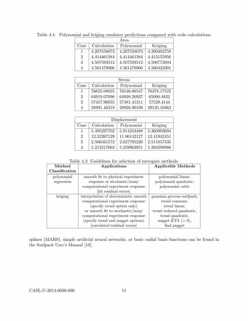
Table 4.1: Polynomial and kriging emulator predictions compared with code calculations.Area
Case Calculation Polynomial Kriging1 4.207558073 4.207558073 4.2094027592 4.414461384 4.414461384 4.4131559563 4.507593512 4.507593512 4.5067738044 4.561478066 4.561478066 4.560423301
StressCase Calculation Polynomial Kriging
1 76625.08025 76546.06547 76378.175222 64919.07096 64938.20937 65000.48323 57457.96055 57481.41311 57529.41444 28991.46319 28938.90198 29135.16863
DisplacementCase Calculation Polynomial Kriging
1 5.495297702 5.914253488 5.3609936942 12.52267129 11.96142127 12.419424513 2.506561572 2.627795226 2.5118575354 5.213217663 5.259963951 5.260298986
Table 4.2: Guidelines for selection of surrogate methods.Method Applications Applicable Methods
Classificationpolynomial smooth fit to physical experiment polynomial linear,regression response or stochastic/noisy polynomial quadratic,
computational experiment response polynomial cubic[iid residual errors]
kriging interpolation of deterministic smooth gaussian process surfpack,computational experiment response trend constant,
(specify trend option only) trend linear,or smooth fit to stochastic/noisy trend reduced quadratic,
computational experiment response trend quadratic,(specify trend and nugget options) nugget ETA (> 0),
[correlated residual errors] find nugget
splines (MARS), simple artificial neural networks, or basic radial basis functions can be found inthe Surfpack User’s Manual [10].
CASL-U-2014-0038-000 51
Chapter 5
Optimization and DeterministicCalibration
The objective of optimization algorithms is to minimize (or maximize) an objective function, typ-ically calculated by the user simulation code, subject to constraints on design variables and re-sponses. Examples of optimization goals include:
• Identify system designs with maximal performance; e.g., case geometry that minimizes dragand weight, yet is sufficiently strong and safe.
• Determine operational settings that maximize system performance, e.g., fuel re-loading pat-tern yielding the smoothest nuclear reactor power distribution while maximizing output.
• Identify minimum-cost system designs/operational settings, e.g., delivery network that mini-mizes cost while also minimizing environmental impact.
• Identify best/worst case scenarios, e.g., impact conditions that incur the most damage.
• Calibration: Determine parameter values that maximize agreement between simulation re-sponse and target response.
The last goal is a critical use case for CASL. The calibration (parameter estimation, inverse problem)process involves adjusting input parameters to optimally fit a model to experimental or high-fidelitycomputational model data, find operational settings that best match a prescribed performanceprofile, or determine source terms for an observed phenomenon. Any Dakota optimization methodcan be applied to calibration problems, though some are tailored to efficiently address local leastsquares problem formulations. This chapter emphasizes deterministic model calibration, whilenon-deterministic approaches such as Bayesian methods are treated in Uncertainty Quantification,Chapter 6.
Available optimization approaches in Dakota include well-tested, proven gradient-based, derivative-free local, and global methods for use in science and engineering design applications. Dakotaalso offers more advanced algorithms, e.g., to manage multi-objective optimization or performsurrogate-based minimization (useful for noisy or expensive problems). A more extensive treatmentof these can be found in “Optimization Capabilities,” “Nonlinear Least Squares Capabilities,” and“Surrogate-Based Minimization” chapters of the Dakota User’s Manual [1]. This chapter continuesby introducing optimization terminology needed to select from the available approaches.
CASL-U-2014-0038-000 52

5.1 Terminology and Problem Formulations
This section provides a basic introduction to the mathematical formulation of optimization prob-lems. The primary goal of this section is to introduce terms relating to these topics, and isnot intended to be a description of theory or numerical algorithms. For further details, con-sult [4], [14], [16], [28], and [38].
A general optimization problem is formulated as follows:
minimize: f(x) objective functionover: x ∈ <M design variables
subject to: gL ≤ g(x) ≤ gU nonlinear inequality constraintsh(x) = ht nonlinear equality constraints
aL ≤ Aix ≤ aU linear inequality constraintsAex = at linear equality constraints
xL ≤ x ≤ xU bound constraints
In this formulation, x = [x1, x2, . . . , xM ] is an M -dimensional vector of real-valued design variablesor design parameters. The M -dimensional vectors xL and xU , are the lower and upper bounds,respectively, on the design parameters. These bounds define the allowable values for the elementsof x, and the set of all allowable values is termed the design space or the parameter space. A designpoint or a sample point is a particular set of values within the parameter space.
The optimization goal is to minimize the objective function, f(x), while satisfying the con-straints. Constraints can be categorized as either linear or nonlinear and as either inequality orequality. The nonlinear inequality constraints, g(x), are “2-sided,” in that they have both lowerand upper bounds, gL and gU , respectively. The nonlinear equality constraints, h(x), have targetvalues specified by ht. The linear inequality constraints create a linear system Aix, where Ai isthe coefficient matrix for the linear system. These constraints are also 2-sided as they have lowerand upper bounds, aL and aU , respectively. The linear equality constraints create a linear systemAex, where Ae is the coefficient matrix for the linear system and at are the target values. Theconstraints partition the parameter space into feasible and infeasible regions. A design point is saidto be feasible if and only if it satisfies all of the constraints. Correspondingly, a design point is saidto be infeasible if it violates one or more of the constraints.
Many different methods exist to solve the optimization problem given by Equation 5.1, all ofwhich iterate on x in some manner. That is, an initial value for each parameter in x is chosen,the response quantities, f(x), g(x), h(x), are computed, often by running a simulation, and somealgorithm is applied to generate a new x that will either reduce the objective function, reduce theamount of infeasibility, or both. To facilitate a general presentation of these methods, three criteriawill be used in the following discussion to differentiate them: optimization problem type, searchgoal, and search method.
The optimization problem type can be characterized both by the types of constraints presentin the problem and by the linearity or nonlinearity of the objective and constraint functions. Forconstraint categorization, a hierarchy of complexity exists for optimization algorithms, ranging fromsimple bound constraints, through linear constraints, to full nonlinear constraints. By the natureof this increasing complexity, optimization problem categorizations are inclusive of all constrainttypes up to a particular level of complexity. That is, an unconstrained problem has no constraints,a bound-constrained problem has only lower and upper bounds on the design parameters, a linearly-
CASL-U-2014-0038-000 53
constrained problem has linear constraints (and optionally bound constraints), and a nonlinearly-constrained problem may contain the full range of nonlinear, linear, and bound constraints (thoughmay omit linear or bound constraints if not applicable). If all of the linear and nonlinear constraintsare equality constraints, then this is referred to as an equality-constrained problem, and if all of thelinear and nonlinear constraints are inequality constraints, then this is referred to as an inequality-constrained problem.
Further categorizations can be made based on the linearity of the objective and constraintfunctions. A problem where the objective function and all constraints are linear is called a linearprogramming (LP) problem. These types of problems commonly arise in scheduling, logistics, andresource allocation applications. Likewise, a problem where at least some of the objective andconstraint functions are nonlinear is called a nonlinear programming (NLP) problem. These NLPproblems predominate in engineering applications and are the primary focus of Dakota.
The search goal refers to the ultimate objective of the optimization algorithm, i.e., eitherglobal or local optimization. In global optimization, the goal is to find the design point that givesthe lowest feasible objective function value over the entire parameter space. In contrast, in localoptimization, the goal is to find a design point that is lowest relative to a “nearby” region of theparameter space. In almost all cases, global optimization will be more computationally expensivethan local optimization. Thus, the user must choose an optimization algorithm with an appropriatesearch scope that best fits the problem goals and the computational budget.
The search method refers to the approach taken in the optimization algorithm to locate anew design point that has a lower objective function or is more feasible than the current designpoint. The search method can be classified as either gradient-based or nongradient-based. In agradient-based algorithm, gradients of the response functions are computed to find the directionof improvement. The Hessian (matrix of second derivatives of objectives and constraints withrespect to parameters) can also be used in these methods to identify curvature to identify localminima from maxima. Gradient-based optimization is the search method that underlies manyefficient local optimization methods. However, a drawback to this approach is that gradientscan be computationally expensive, inaccurate, or even nonexistent (the situation for Hessians istypically even worse). In such situations, nongradient-based search methods may be useful. Thereare numerous approaches to nongradient-based optimization. Some of the more well known ofthese include pattern search methods (nongradient-based local techniques) and genetic algorithms(nongradient-based global techniques).
5.1.1 Special Considerations for Calibration
Any Dakota optimization algorithm can be applied to calibration problems arising in parameterestimation, system identification, and test/analysis reconciliation. However, nonlinear least-squaresmethods are optimization algorithms that exploit the special structure of a least squares or sum-of-squares objective function [14]. Here the misfit between vectors of model responses and simulationdata is measured in the Euclidean or two-norm.
To exploit the problem structure, more granularity is needed in the response data than isrequired for a typical optimization problem. That is, rather than using the sum-of-squares objectivefunction and its gradient, least-squares iterators require each term used in the sum-of-squaresformulation along with its gradient. This means that the functions in the Dakota response data setconsist of the N individual least-squares terms along with any nonlinear inequality and equalityconstraints. These individual terms are often called residuals when they denote differences of
CASL-U-2014-0038-000 54

observed quantities from values computed by the model whose parameters are being estimated.The enhanced granularity needed for nonlinear least-squares algorithms allows for simplified
computation of an approximate Hessian matrix. In Gauss-Newton-based methods for example,the true Hessian matrix is approximated by neglecting terms in which residuals multiply Hessians(matrices of second partial derivatives) of residuals, under the assumption that the residuals arezero in expected value under the nonlinear least-squares model. As a result, residual function valueand gradient information (first-order information) is sufficient to define the value, gradient, andapproximate Hessian of the sum-of-squares objective function (second-order information).
In practice, least-squares solvers will tend to be significantly more efficient than general-purposeoptimization algorithms when the Hessian approximation is a good one, i.e., when the neglectedcomponent has negligible effect at the solution. Specifically, they can exhibit the quadratic con-vergence rates of full Newton methods, even though only first-order information is used. Gauss-Newton-based least-squares solvers may experience difficulty when the residuals at the solution aresignificant. Dakota has three solvers customized to take advantage of the sum of squared residualsstructure in this problem formulation. Least squares solvers may experience difficulty when theresiduals at the solution are significant, although experience has shown that Dakota’s NL2SOLmethod can handle some problems that are highly nonlinear and have nonzero residuals at thesolution.
Specialized least squares solution algorithms can exploit the structure of a sum-of-squares ob-jective function for problems of the form:
minimize: f(θ) =∑N
i=1[Ti(θ)]2 =∑N
i=1[yi(θ)− di]2 least squares objective functionover: θ ∈ <M calibration variables
subject to: gL ≤ g(x) ≤ gU nonlinear inequality constraintsh(θ) = ht nonlinear equality constraints
aL ≤ Aiθ ≤ aU linear inequality constraintsAeθ = at linear equality constraints
θL ≤ θ ≤ θU bound constraints
where f(θ) is the objective function to be minimized and Ti(θ) is the i-th least squares term. Thebound, linear, and nonlinear constraints are the same as described previously for (5.1). Specializedleast squares algorithms are generally based on the Gauss-Newton approximation. When differen-tiating f(θ) twice, terms of Ti(θ)T ′′i (θ) and [T ′i (θ)]
2 result. Because Ti(θ) is zero in expected valueunder the nonlinear least-squares model, the Hessian matrix of second derivatives of f(θ) can beapproximated using only first derivatives of Ti(θ). As a result, Gauss-Newton algorithms exhibitquadratic convergence rates near the solution for those cases when the Hessian approximation isaccurate, i.e. the neglected component has negligible effect at the solution. Thus, by exploiting thestructure of the problem, the second order convergence characteristics of a full Newton algorithmcan be obtained using only first order information from the least squares terms. For problems withnonsmooth gradients or poor finite difference approximations, see [21].
A common example for Ti(θ) might be the difference between experimental data and modelpredictions for a response quantity at a particular location and/or time step, i.e.:
Ti(θ) = yi(θ)− diwhere yi(θ) is the response quantity predicted by the model and di is the corresponding experimentaldata. In this case, θ would have the meaning of model parameters which are not precisely known
CASL-U-2014-0038-000 55

and are being calibrated to match available data. This class of problem is known by the termsparameter estimation, system identification, model calibration and test/analysis reconciliation, forexample.
This overview of optimization problem formulations and goals approaches underscores that nosingle optimization method or algorithm works best for all types of optimization problems. Thefollowing section offers some basic guidelines for choosing one for specific optimization problems.
5.2 Recommended Methods
In selecting an optimization method, important considerations include the type of variables inthe problem (continuous, discrete, mixed), whether a global search is needed or a local search issufficient, and the required constraint support (unconstrained, bound constrained, or generally con-strained). Less obvious, but equally important, considerations include the efficiency of convergenceto an optimum (i.e., convergence rate) and the robustness of the method in the presence of chal-lenging design space features (e.g., nonsmoothness). Sensitivity analysis (described in Chapter 3) isa critical precursor to assess problem characteristics prior to choosing and applying an optimizationmethod.
For example the cantilever beam optimization problem posed in (2.3) in Section 2.1 has con-tinuous design variables only, nonlinear inequality constraints, and bound constraints. Sensitivityanalysis in Section 3.2 indicated that the objective and constraints are smooth functions of thedesign variables. This can also be directly inferred from the algebraic physics equations for thecantilever beam (2.1), though cannot for a general physics simulation.
Table 5.1 highlights a few key Dakota optimization approaches and problems for which theyare suited. The following sections offer more details on the approaches and input file examples.Without considering specific problem knowledge or characteristics, a derivative-free local patternsearch approach is typically a good starting point. If it doesn’t find good solutions, move to agenetic algorithm. If it is too costly, move to a surrogate-based approach. However, when problemsare smooth and not too multimodal, a local algorithm will outperform these other approaches.
5.2.1 Gradient-Based Local Methods
Gradient-based optimizers are best suited for efficient navigation to a local minimum in the vicinityof the initial point. They are not intended to find global optima in nonconvex design spaces. Forglobal optimization methods, see Section 5.2.3. Gradient-based optimization methods are highlyefficient, with the best convergence rates of all of the local optimization methods, and are the meth-ods of choice when the problem is smooth, unimodal, and well-behaved. However, these methodscan be among the least robust when a problem exhibits nonsmooth, discontinuous, or multimodalbehavior. Figure 5.1 depicts a multimodal function on which gradient-based optimizers will typi-cally find only a nearby local minimum. The derivative-free methods described in Section 5.2.2 aremore appropriate for problems with some of these characteristics.
Newton methods are representative of gradient-based optimization methods. These can bederived by applying Newton’s method for root finding to ∇f(x) = 0 to find a local minimum of theobjective function. The resulting progression from current iterate xn to next iterate xn+1 is then
xn+1 = xn −(∇2f(xn)
)−1∇f(xn).
CASL-U-2014-0038-000 56
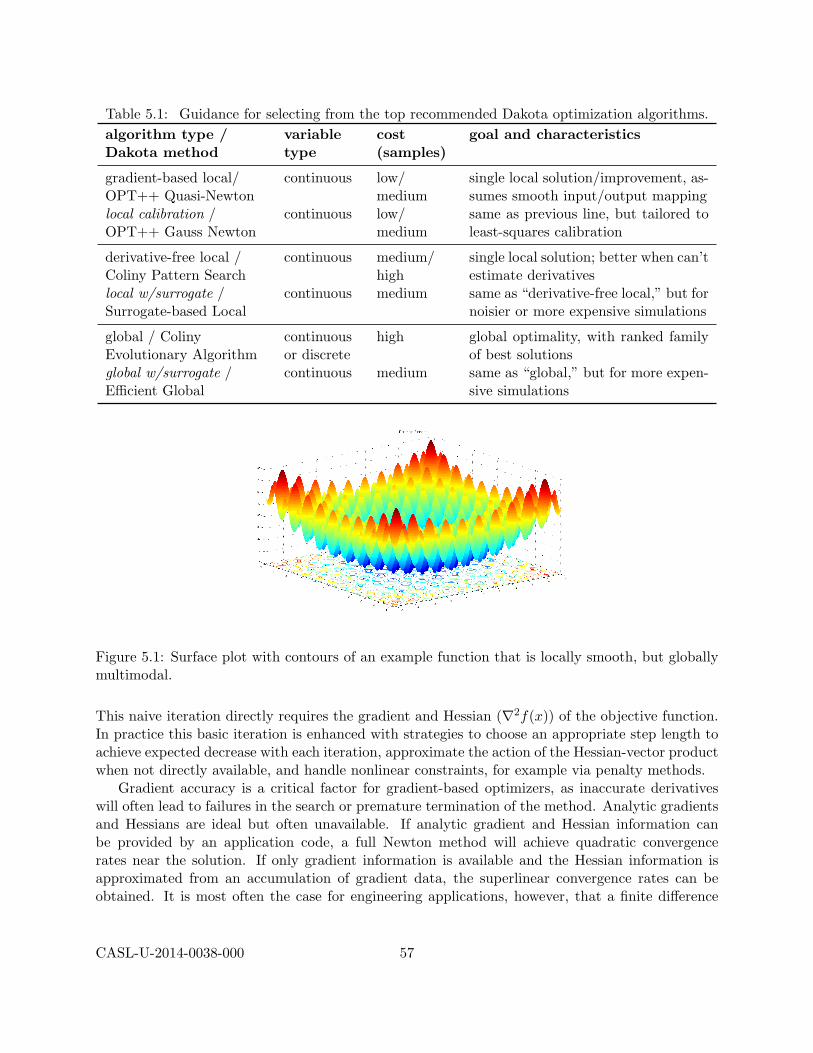
Table 5.1: Guidance for selecting from the top recommended Dakota optimization algorithms.algorithm type /Dakota method
variabletype
cost(samples)
goal and characteristics
gradient-based local/OPT++ Quasi-Newton
continuous low/medium
single local solution/improvement, as-sumes smooth input/output mapping
local calibration /OPT++ Gauss Newton
continuous low/medium
same as previous line, but tailored toleast-squares calibration
derivative-free local /Coliny Pattern Search
continuous medium/high
single local solution; better when can’testimate derivatives
local w/surrogate /Surrogate-based Local
continuous medium same as “derivative-free local,” but fornoisier or more expensive simulations
global / ColinyEvolutionary Algorithm
continuousor discrete
high global optimality, with ranked familyof best solutions
global w/surrogate /Efficient Global
continuous medium same as “global,” but for more expen-sive simulations
Figure 5.1: Surface plot with contours of an example function that is locally smooth, but globallymultimodal.
This naive iteration directly requires the gradient and Hessian (∇2f(x)) of the objective function.In practice this basic iteration is enhanced with strategies to choose an appropriate step length toachieve expected decrease with each iteration, approximate the action of the Hessian-vector productwhen not directly available, and handle nonlinear constraints, for example via penalty methods.
Gradient accuracy is a critical factor for gradient-based optimizers, as inaccurate derivativeswill often lead to failures in the search or premature termination of the method. Analytic gradientsand Hessians are ideal but often unavailable. If analytic gradient and Hessian information canbe provided by an application code, a full Newton method will achieve quadratic convergencerates near the solution. If only gradient information is available and the Hessian information isapproximated from an accumulation of gradient data, the superlinear convergence rates can beobtained. It is most often the case for engineering applications, however, that a finite difference
CASL-U-2014-0038-000 57
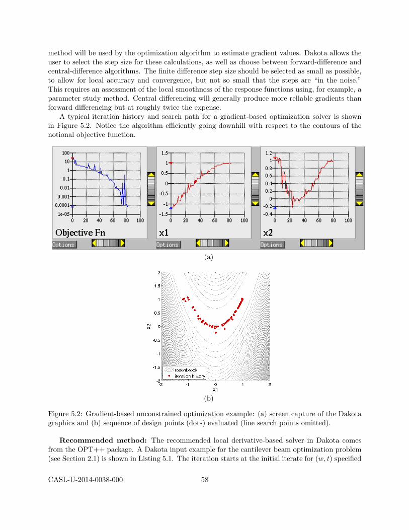
method will be used by the optimization algorithm to estimate gradient values. Dakota allows theuser to select the step size for these calculations, as well as choose between forward-difference andcentral-difference algorithms. The finite difference step size should be selected as small as possible,to allow for local accuracy and convergence, but not so small that the steps are “in the noise.”This requires an assessment of the local smoothness of the response functions using, for example, aparameter study method. Central differencing will generally produce more reliable gradients thanforward differencing but at roughly twice the expense.
A typical iteration history and search path for a gradient-based optimization solver is shownin Figure 5.2. Notice the algorithm efficiently going downhill with respect to the contours of thenotional objective function.
(a)
(b)
Figure 5.2: Gradient-based unconstrained optimization example: (a) screen capture of the Dakotagraphics and (b) sequence of design points (dots) evaluated (line search points omitted).
Recommended method: The recommended local derivative-based solver in Dakota comesfrom the OPT++ package. A Dakota input example for the cantilever beam optimization problem(see Section 2.1) is shown in Listing 5.1. The iteration starts at the initial iterate for (w, t) specified
CASL-U-2014-0038-000 58

in initial point on line 16. The state variables are held fixed at their given values. The algorithmseeks to minimize the cantilever objective function (area), within the bound constraints specified onlines 15 and 17, subject to constraints on stress and displacement specified on line 30. The algorithmwill terminate when the convergence criteria from lines 7 and 8 are met. Notice the responses sectionspecifies numerical gradients (line 32), indicating that Dakota should approximate the derivativesof model responses with respect to parameters via finite differences. If the response is a rough orstrongly nonlinear function of the parameters, these approximations can be poor and yield badperformance or results. Figure 5.3 shows an excerpt of the Dakota output, showing the optimaldesign point found.
Listing 5.1: Dakota input file showing local gradient-based optimization on the cantilever beamproblem.strategy
2 single_method
tabular_graphics_data
4 tabular_graphics_file ’cantilever_opt_grad.dat ’
6 method
optpp_q_newton
8 convergence_tolerance 1.0e-4
constraint_tolerance 1.0e-1
10
model
12 single
14 variables
continuous_design = 2
16 upper_bounds 4.0 4.0
initial_point 2.4 3.5
18 lower_bounds 1.0 1.0
descriptors ’w’ ’t’
20 continuous_state = 4
initial_state 40000. 29.E+6 500. 1000.
22 descriptors ’R’ ’E’ ’X’ ’Y’
24 interface
direct
26 analysis_driver = ’mod_cantilever ’
28 responses
objective_functions = 1
30 # constraints assumed <= 0 unless bounds given
nonlinear_inequality_constraints = 2
32 descriptors = ’area ’ ’stress ’ ’displacement ’
numerical_gradients forward
34 fd_step_size 1.0e-6
no_hessians
Variation for calibration: Listing 5.2 shows the Dakota input variation to directly treatcalibration with a least-squares specific gradient-based solver. This example tunes the active vari-ables (line 14) θ = (E,w, t) to match synthetic experimental data from a file, with (line 30) or
CASL-U-2014-0038-000 59

<<<<< Function evaluation summary: 18 total (18 new, 0 duplicate)<<<<< Best parameters =
2.4000000000e+00 w3.5000000000e+00 t4.0000000000e+04 R2.9000000000e+07 E5.0000000000e+02 X1.0000000000e+03 Y
<<<<< Best objective function =8.4000000000e+00
<<<<< Best constraint values =-4.7108843537e+03-2.9685051703e-01
Figure 5.3: Dakota output showing optimal local gradient-based optimization result for cantileverbeam.
without (line 31) added noise. The data were generated using the following tuning parametervalues: E = 2.85E7, w = 2.5, t = 3.0, and fixed state parameter values: R = 40000, X = 500,Y = 1000. The input file specifies calibration terms instead of objective functions at line29, indicating to Dakota that it should treat these responses as terms in a least-squares calibrationproblem. The data here is a set of three observations, one each for area, stress, and displacement.The NL2SOL solver is used for this example as it performs better than the default-recommendedOPT++ Gauss-Newton solver.
The calibrated parameter values from the Dakota output are shown in Figure 5.4. Dakota hasrecovered the true values of the parameters, verifying the operation of the algorithm. The outputfrom local calibration methods also includes confidence intervals on the parameters. With 95%confidence the true value of each parameter lies in the interval specified, given the misfit betweenthe model and corresponding data. When this problem is exercised with noisy data, the confidenceintervals expectedly grow larger.
For problems not suitable for local gradient-based optimization, any of the optimization methodsdiscussed in the following sections can be applied to Dakota responses with calibration terms.Dakota will automatically compute the objective function as the sum of squared residuals forpresentation to the optimization algorithm.
5.2.2 Derivative-Free Local Methods
Derivative-free methods can be more robust and more inherently parallel than gradient-based ap-proaches. They can be applied in situations were gradient calculations are too expensive or un-reliable. In addition, some derivative-free methods can be used for global optimization whichgradient-based techniques (see 5.2.1), by themselves, cannot. For these reasons, derivative-freemethods are often go-to methods when the problem may be nonsmooth, multimodal, or poorlybehaved. It is important to be aware, however, that they exhibit much slower convergence ratesfor finding an optimum, and as a result, tend to be much more computationally demanding thangradient-based methods. They often require from several hundred to a thousand or more function
CASL-U-2014-0038-000 60

Listing 5.2: Dakota input file showing deterministic local calibration with a least-squares solver onthe cantilever beam problem.
1 strategy
single_method
3 tabular_graphics_data
tabular_graphics_file ’cantilever_calibration.dat ’
5
7 method
nl2sol
9 convergence_tolerance 1.0e-6
# output verbose
11
model
13 single
15 variables
active design
17 continuous_design 3
upper_bounds 31000000 10 10
19 initial_point 29000000 4 4
lower_bounds 27000000 1 1
21 descriptors ’E’ ’w’ ’t’
continuous_state 3
23 initial_state 40000 500 1000
descriptors ’R’ ’X’ ’Y’
25
interface
27 direct
analysis_driver = ’mod_cantilever ’
29
responses
31 calibration_terms 3
calibration_data_file = ’dakota_cantilever_examples.clean.dat ’
33 #calibration_data_file = ’dakota_cantilever_examples.error.dat ’
freeform
35 descriptors = ’area ’ ’stress ’ ’displacement ’
analytic_gradients
37 no_hessians
CASL-U-2014-0038-000 61

<<<<< Function evaluation summary: 18 total (17 new, 1 duplicate)<<<<< Best parameters =
2.8499999995e+07 E2.5000000002e+00 w2.9999999997e+00 t4.0000000000e+04 R5.0000000000e+02 X1.0000000000e+03 Y
<<<<< Best residual norm = 2.9442886479e-06; 0.5 * norm^2 = 4.3344178210e-12<<<<< Best residual terms =
-2.3943602656e-102.9442885534e-067.0639355476e-10
<<<<< Best data captured at function evaluation 17
Confidence Interval for E is [ 2.8499511022e+07, 2.8500488969e+07 ]Confidence Interval for w is [ 2.4999189436e+00, 2.5000810568e+00 ]Confidence Interval for t is [ 2.9999176961e+00, 3.0000823033e+00 ]
Figure 5.4: Dakota output showing optimal local gradient-based calibration result for cantileverbeam, clean data.
evaluations for local methods, depending on the number of variables, and may require from thou-sands to tens-of-thousands of function evaluations for global methods. Given the computationalcost, it is often prudent to use derivative-free methods to identify regions of interest and then usegradient-based methods to hone in on the solution. In addition to slow convergence, nonlinearconstraint support in derivative-free methods is an open area of research and, while supported bymany methods in Dakota, is not as refined as constraint support in gradient-based methods.
Local pattern search algorithms work by sampling the objective function at points on a stencil,often chosen to align with the coordinate axes. The stencil moves, expands, and contracts as thealgorithm progresses. A typical pattern search iteration history is provided in Figures 5.5(a) and(b), which show the locations of the function evaluations used in the pattern search algorithm.Figure 5.5(c) provides a close-up view of the pattern search function evaluations used at the startof the algorithm (from a starting point (x1, x2) = (0.0, 0.0). The coordinate pattern is clearly visibleat the start of the iteration history, and the decreasing size of the coordinate pattern is evident atthe design points move toward (x1, x2) = (1.0, 1.0).
While pattern search algorithms are useful in many optimization problems, this example showssome of the drawbacks to this algorithm. While a pattern search method may make good initialprogress towards an optimum, it is often slow to converge, here not fully converging after 2000iterations. On a smooth, differentiable function such as that depicted, a nongradient-based methodwill not be as efficient as a gradient-based method. However, there are many engineering designapplications where gradient information is inaccurate or unavailable, which renders gradient-basedoptimizers ineffective. Thus, pattern search algorithms are often good choices in complex engineer-ing applications when the quality of gradient data is suspect.
Recommended method: We recommend the Coliny Pattern Search algorithm for a derivative-
CASL-U-2014-0038-000 62

(a)
(b) (c)
Figure 5.5: Pattern search optimization example: (a) screen capture of the Dakota graphics, (b)sequence of design points (dots) evaluated and (c) close-up view illustrating the shape of thecoordinate pattern used.
free local method. A Dakota input file shown in Listing 5.3 applies a pattern search method tothe cantilever beam optimization problem to minimize the objective function (area), subject toconstraints on stress and displacement (see Section 2.1). The input is similar to the input file forthe gradient-based optimization, except it has a different set of keywords in the method block ofthe input file (line 6–15), and the gradient specification in the responses block has been changed tono gradients (line 39). The pattern search optimization algorithm used, coliny pattern searchis part of the SCOLIB library [17]. See the Dakota Reference Manual [2] for more information onthe method block commands that can be used with SCOLIB algorithms.
The tailing portion of the Dakota output shows the final design point and constraint values; seeFigure 5.6. A solution similar to the gradient-based approach was found, though the constraint fordisplacement was slightly violated (this can often be addressed through larger constraint penalties inderivative-free methods; see commented option in the input file). However, the algorithm requiredabout an order of magnitude more function evaluations.
CASL-U-2014-0038-000 63

Listing 5.3: Dakota input file showing local derivative-free optimization on the cantilever beamproblem.strategy
2 single_method
tabular_graphics_data
4 tabular_graphics_file ’cantilever_opt_ps.dat ’
6 method
max_iterations = 1000
8 max_function_evaluations = 2000
coliny_pattern_search
10 solution_accuracy = 1e-4
initial_delta = 0.5
12 threshold_delta = 1e-4
exploratory_moves basic_pattern
14 contraction_factor = 0.75
# constraint_penalty = 10000
16
model
18 single
20 variables
continuous_design = 2
22 upper_bounds 4.0 4.0
initial_point 2.5 2.5
24 lower_bounds 1.0 1.0
descriptors ’w’ ’t’
26 continuous_state = 4
initial_state 40000. 29.E+6 500. 1000.
28 descriptors ’R’ ’E’ ’X’ ’Y’
30 interface
direct
32 analysis_driver = ’mod_cantilever ’
34 responses
objective_functions = 1
36 # constraints assumed <= 0 unless bounds given
nonlinear_inequality_constraints = 2
38 descriptors = ’area ’ ’stress ’ ’displacement ’
no_gradients
40 no_hessians
CASL-U-2014-0038-000 64

<<<<< Function evaluation summary: 149 total (149 new, 0 duplicate)<<<<< Best parameters =
2.3875000000e+00 w3.2493181357e+00 t4.0000000000e+04 R2.9000000000e+07 E5.0000000000e+02 X1.0000000000e+03 Y
<<<<< Best objective function =7.7577470490e+00
<<<<< Best constraint values =-1.6832688252e-014.1748455156e-02
<<<<< Best data captured at function evaluation 142
Figure 5.6: Dakota output showing results from local derivative-free optimization with a patternsearch algorithm.
5.2.3 Derivative-Free Global Methods
Dakota has a number of global optimization algorithms, including DiRECT, genetic algorithms,and surrogate-based approaches. Here we discuss genetic algorithms. In contrast to pattern searchalgorithms, which are local optimization methods, evolutionary algorithms (EA) are global opti-mization methods. EAs are best suited to optimization problems that have multiple local optima,and where gradients are either too expensive to compute or are not readily available.
Evolutionary algorithms work by generating an initial random sample in the parameter space,computing function values/constraints at those points, and then determining the next places tosample based on biological genetic selection principles of mutation and fitness. A simplified evolu-tionary or genetic algorithm for optimization would include:
1. Initialize a random population (sample) of individual x values.
2. Evaluate the fitness with respect to optimization objective and constraints.
3. Select more fit individuals as parents to reproduce.
4. Recombine and mutate to create a new population.
5. Iterate to (2.) until convergence is reached.
Here the implementation details of each step, for example how to select parents, how to combine andmutate, vary greatly among implementations, but are usually biologically inspired. Figure 5.7(a)shows the population of 50 randomly selected design points that comprise the first generation ofthe EA, and Figure 5.7(b) shows the final population of 50 design points, where most of the 50points are clustered near (x1, x2) = (0.98, 0.95).
Listing 5.4 shows a Dakota input file that uses an EA to solve the cantilever beam optimizationproblem as described in Section 2.1. Each generation of the EA has a population size of 50 (line 11).
CASL-U-2014-0038-000 65

(a) (b)
Figure 5.7: Evolutionary algorithm optimization example: 50 design points in the (a) initial and(b) final populations selected by the evolutionary algorithm.
The algorithm will take at most 100 iterations comprising no more than 2000 function evaluations(lines 7 and 8). The EA software available in Dakota provides the user with much flexibility inchoosing the settings used in the optimization process. The details of all the settings are notdiscussed here; see [2] and [17].
On completion, the file cantilever opt ea.dat provides a listing of the design parametervalues and objective function values for all 2,000 design points evaluated during the running of theEA. The final solution is shown in Figure 5.8.
<<<<< Function evaluation summary: 2007 total (2007 new, 0 duplicate)<<<<< Best parameters =
2.3547960771e+00 w3.3249245714e+00 t4.0000000000e+04 R2.9000000000e+07 E5.0000000000e+02 X1.0000000000e+03 Y
<<<<< Best objective function =7.8295193371e+00
<<<<< Best constraint values =-6.8024421496e+02-3.4463344891e-03
<<<<< Best data captured at function evaluation 1982
Figure 5.8: Dakota output showing optimal point found by a global evolutionary algorithm.
EAs are better suited to optimization problems where conventional gradient-based optimizationfails, such as situations where there are multiple local optima and/or gradients are not available. In
CASL-U-2014-0038-000 66
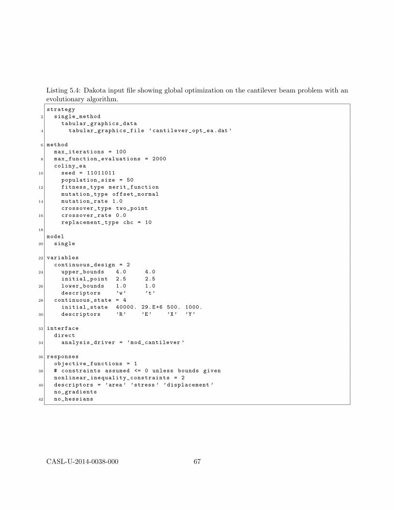
Listing 5.4: Dakota input file showing global optimization on the cantilever beam problem with anevolutionary algorithm.strategy
2 single_method
tabular_graphics_data
4 tabular_graphics_file ’cantilever_opt_ea.dat ’
6 method
max_iterations = 100
8 max_function_evaluations = 2000
coliny_ea
10 seed = 11011011
population_size = 50
12 fitness_type merit_function
mutation_type offset_normal
14 mutation_rate 1.0
crossover_type two_point
16 crossover_rate 0.0
replacement_type chc = 10
18
model
20 single
22 variables
continuous_design = 2
24 upper_bounds 4.0 4.0
initial_point 2.5 2.5
26 lower_bounds 1.0 1.0
descriptors ’w’ ’t’
28 continuous_state = 4
initial_state 40000. 29.E+6 500. 1000.
30 descriptors ’R’ ’E’ ’X’ ’Y’
32 interface
direct
34 analysis_driver = ’mod_cantilever ’
36 responses
objective_functions = 1
38 # constraints assumed <= 0 unless bounds given
nonlinear_inequality_constraints = 2
40 descriptors = ’area ’ ’stress ’ ’displacement ’
no_gradients
42 no_hessians
CASL-U-2014-0038-000 67

such cases, the computational expense of an EA is warranted since other optimization methods arenot applicable or impractical. In many optimization problems, EAs often quickly identify promisingregions of the design space where the global minimum may be located. However, an EA can beslow to converge to the optimum. For this reason, it can be an effective approach to combine theglobal search capabilities of an EA with the efficient local search of a gradient-based algorithm ina hybrid optimization strategy. In this approach, the optimization starts by using a few iterationsof an EA to provide the initial search for a good region of the parameter space (low objectivefunction and/or feasible constraints), and then it switches to a gradient-based algorithm (using thebest design point found by the EA as its starting point) to perform an efficient local search for anoptimum design point. More information on this hybrid approach is provided in the “Strategy”chapter of the Dakota User’s Manual [1].
Another effective method for global optimization, especially for costlier computational models,is the Efficient Global Optimization (EGO) approach. This is discussed in the section “EfficientGlobal Minimization” of the Dakota User’s Manual [1].
5.3 Summary and Additional Approaches
In selecting an optimization method, important considerations include the type of variables inthe problem (continuous, discrete, mixed), whether a global search is needed or a local searchis sufficient, and the required constraint support (unconstrained, bound constrained, or generallyconstrained). Less obvious, but equally important, considerations include the efficiency of conver-gence to an optimum (i.e., convergence rate) and the robustness of the method in the presence ofchallenging design space features (e.g., nonsmoothness).
Table 5.2 provides a more extensive reference for selecting from among all of Dakota’s optimiza-tion methods. Here blank fields inherit the values from above. With respect to constraint support,the methods with more advanced constraint support are also applicable to the lower constraintsupport levels; they are listed only at their highest level of constraint support for brevity. Forexample, all methods listed as supporting nonlinear constraints also support bound constraints.
Because of the computational cost of running simulation models, surrogate-based optimization(SBO) methods are often used to reduce the number of actual simulation runs. In SBO, a surrogateor approximate model is automatically constructed by Dakota based on a limited number of simu-lation runs. The optimization is then performed on the surrogate model. Dakota has an extensiveframework for managing a variety of local, multipoint, global, and hierarchical surrogates for usein optimization. Finally, sometimes there are multiple objectives that one may want to optimizesimultaneously instead of a single scalar objective. In this case, one may employ multi-objectivemethods described in “Optimization Capabilities” in the Dakota User’s Manual to either form asingle composite objective, or assess the trade-off between multiple objectives directly.
CASL-U-2014-0038-000 68

Table 5.2: Detailed guidelines for selecting from among all Dakota optimization methods. Blankfields inherit the values from above.
Method Desired Problem Applicable MethodsClassification Characteristics
smooth; continuous variables optpp cgno constraints
smooth; continuous variables; dot bfgs, dot frcg, conmin frcgbound constraints
Gradient-Based smooth; continuous variables; npsol sqp, nlpql sqp, dot mmfd,Local bound constraints, dot slp, dot sqp, conmin mfd,
linear and nonlinear constraints optpp newton, optpp q newton,optpp fd newton,
weighted sums (multiobjective),pareto set strategy (multiobjective)
Gradient-Based smooth; continuous variables; hybrid strategy,Global bound constraints, multi start strategy
linear and nonlinear constraints
nonsmooth; continuous variables; optpp pdsbound constraints
nonsmooth; continuous variables; asynch pattern search,Derivative-Free bound constraints, coliny cobyla, coliny pattern search,
Local linear and nonlinear constraints coliny solis wets,surrogate based local
nonsmooth; continuous variables;discrete variables; bound constraints, mesh adaptive search
nonlinear constraints
nonsmooth; continuous variables; ncsu directbound constraints
nonsmooth; continuous variables; coliny direct, efficient global,Derivative-Free bound constraints, surrogate based global
Global linear and nonlinear constraints
nonsmooth; continuous variables, coliny ea, soga,discrete variables; bound constraints, moga (multiobjective)
linear and nonlinear constraints
CASL-U-2014-0038-000 69
Chapter 6
Uncertainty Quantification
At a high level, uncertainty quantification (UQ) constitutes the process of characterizing input,numerical, and experimental uncertainties – consisting of both measurement errors and variabilityin replicate data, propagating these uncertainties through a computational model, and performingstatistical or interval assessments on the resulting responses. This process determines the effect ofuncertainties and assumptions on model responses or quantities of interest (QoI). In Section 6.1,we summarize techniques to propagate input uncertainties through models whereas in Section 6.2,we discuss Bayesian techniques to quantify input uncertainties.
For this discussion, inputs collectively refer to model parameters, initial conditions, boundaryconditions, or exogenous forces. For models in which inputs are derived from closure, constitutiveor phenomenological relations, one must employ model calibration techniques to estimate means,moments, or ultimately probability density functions (PDF) for these calibrated inputs based onexperimental data or high-fidelity codes. This is often termed inverse uncertainty quantification.For CASL applications, inputs requiring calibration include cross-section values, closure and phe-nomenological parameters, and initial and boundary conditions.
The quantification of response or output uncertainties facilitates optimal design and decisionmaking and is necessary to ensure robustness, performance or safety margins. For example, outputsspecified for emergency core cooling systems include peak clad temperatures and maximum localcladding oxidation. The manner in which output statistics are employed depends on the application.For the assessment of design margins, the sample mean x and sample variance s2 can be used toconstruct 2σ confidence intervals x± 2s whereas a predictive distribution for the output might becompared to replicate data to assess validation.
Wilks’ formula constitutes a classical approach for assessing output uncertainty [29, 41]. In thiscoverage approach, the code is run N times for randomly selected input values chosen from expert-specified intervals. The outputs are then ranked to establish tolerance bounds for the response.This approach has the advantage that the number of required code evaluations is independent ofthe number of parameters. However, the resulting tolerance bounds can be overly conservative andthe techniques detailed in Sections 6.1 and 6.2 yield more precise bounds or densities for inputsand outputs.
UQ is related to the sensitivity analysis, detailed in Chapter 3, in that the common goal is togain an understanding of how variations in the parameters or inputs affect the response functionsof the engineering design problem. However, for UQ, some or all of the components of the param-eter vector are considered to be uncertain as specified by particular probability distributions (e.g.,
CASL-U-2014-0038-000 70

normal, exponential, extreme value), or other uncertainty structures. By assigning specific distri-butional structure to the inputs, distributional structure for the outputs (i.e., response statistics)can be inferred. UQ can thus be defined as the process of quantifying the imprecision of computedmodel responses or quantities of interest whereas sensitivity analysis ascertains how uncertainty inmodel outputs can be apportioned to uncertainties in model inputs when taken either singly or incombination over the range of input values.
6.1 Uncertainty Propagation
Whereas Dakota provides a number of options for propagating uncertainties through models, wefocus on sampling and stochastic polynomial methods. The selection of these techniques to employcan be based on the following criteria:
• Sampling methods are applicable for nonsmooth and/or multi-modal response functions andgeneral input densities including those for correlated parameters, initial conditions, boundaryconditions or exogenous forces. Since sampling methods require numerous model evaluations– e.g., hundreds to millions – they necessitate that models be efficient to evaluate or requirethe use of suitable surrogate models. Sampling methods yield response samples, which can bepost-processed – e.g., using kernel density estimation (kde) routines – to construct responsedensities.
• Stochastic polynomial methods require smooth response functions. Stochastic collocation(SC) methods are applicable for general input densities whereas nonintrusive polynomialchaos expansions (PCE) require the specification or construction of orthogonal polynomials.For normal or uniform input densities, Hermite or Legendre polynomials are employed. Fordensities that do not correspond to members in the Askey family of polynomials, Dakotaprovides the capability of employing empirical histograms to generate orthogonal polynomials.Evaluation of the quantity of interest often necessitates that inputs are mutually independent,which is generally not the case, but can often be achieved through Nataf transformations.These methods utilize Dakota sparse grid routines to provide highly efficient evaluation ofresponse moments and Sobol global sensitivity indices.
We note that Dakota provides a number of other techniques – including local and global relia-bility methods, interval methods, and mixed UQ algorithms – to propagate uncertainties throughmodels. Readers are referred to the “Uncertainty Quantification Capabilities” chapter of [1] fordetails about these methods.
We do not differentiate between aleatoric uncertainties, which are inherent to a problem orexperiments and are intrinsically probabilistic in nature, and epistemic uncertainties, which aredue to lack of knowledge. We refer readers to [34] for details regarding the nature of these un-certainties and to the “Uncertainty Quantification Capabilities” chapter of [1] for a description ofhow Dakota algorithms accommodate these two classes of uncertainties. Further details regardingvarious uncertainty propagation techniques are provided in [34, 37].
6.1.1 Sampling Methods
Sampling-based methods are the most robust uncertainty techniques available, are applicable toalmost all simulations, and possess rigorous error bounds. Consequently, they should be used when-
CASL-U-2014-0038-000 71
ever the function is relatively inexpensive to compute and adequate sampling can be performed. Inthe case of computationally expensive simulations, however, the number of function evaluations re-quired by traditional techniques such as Monte Carlo and Latin hypercube sampling (LHS) quicklybecomes prohibitive, especially if tail statistics are needed. We note that the issues associated withtail statistics can be mitigated through the use of importance sampling.
Alternatively, one can apply the traditional sampling techniques to a surrogate function ap-proximating the expensive computational simulation. However, if this approach is selected, theuser should be aware that it is difficult to assess the accuracy of the results. Unlike the case ofsurrogate-based local minimization, there is no simple pointwise calculation to verify the accuracyof the approximate results. This is due to the functional nature of uncertainty quantification; i.e.,the accuracy of the surrogate over the entire parameter space needs to be considered, not justaround a candidate optimum as in the case of surrogate-based local optimization. This issue es-pecially manifests itself when trying to estimate low probability events such as the catastrophicfailure of a system.
Due to the computational complexity of CASL codes, sampling methods will generally needto be applied to surrogate models rather than physics-based codes. Hence the issues associatedwith establishing the accuracy of the surrogate must be addressed or the accuracy of the surrogate-based sampling results verified for these codes. Techniques to establish surrogate accuracy include“leave-one-out” cross-validation for Gaussian processes [6] and the Dakota K-fold cross-validationcapability, which includes “leave-one-out.” Details regarding the use of the Dakota sampling capa-bility are provided in Section 6.1.5.
6.1.2 Stochastic Polynomial Methods
Stochastic polynomial methods comprise a second class of forward propagation techniques, whichare available in Dakota. The development of these techniques mirrors that of deterministic Galerkinand finite element analysis utilizing the notions of projection, collocation, orthogonality, and weakconvergence [12, 13]. Rather than providing point estimates, they form an approximation to thefunctional relationship between random inputs and response functions, which provides a represen-tation of output uncertainties for multi-code simulations. Expansion methods include nonintrusivepolynomial chaos expansions (PCE), which employ multivariate orthogonal polynomials that aretailored to particular input probability distributions, and stochastic collocation (SC), which em-ploys multivariate interpolation polynomials.
For certain applications, sampling-based models can be efficiently combined with stochasticpolynomial methods. For example, it is often advantageous to employ Latin hypercube samplingto construct a surrogate, which is subsequently employed with a regression-based nonintrusivepolynomial chaos expansion.
Nonintrusive Polynomial Chaos Expansions (PCE)
To motivate nonintrusive PCE methods, which for certain implementation regimes are alsotermed pseudo-spectral or discrete projection methods, we consider a parameter-dependent responseY (X) where X ∈ <M . For random inputs X, this response is represented by the truncatedexpansion
Y (X) =J∑j=0
αjΨj(X) (6.1)
CASL-U-2014-0038-000 72
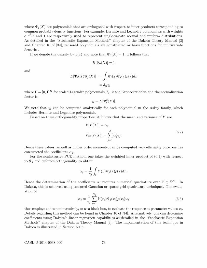
where Ψj(X) are polynomials that are orthogonal with respect to inner products corresponding tocommon probably density functions. For example, Hermite and Legendre polynomials with weightse−x2/2 and 1 are respectively used to represent single-variate normal and uniform distributions.As detailed in the “Stochastic Expansion Methods” chapter of the Dakota Theory Manual [3]and Chapter 10 of [34], tensored polynomials are constructed as basis functions for multivariatedensities.
If we denote the density by ρ(x) and note that Ψ0(X) = 1, if follows that
E[Ψ0(X)] = 1
andE[Ψi(X)Ψj(X)] =
∫Γ
Ψi(x)Ψj(x)ρ(x)dx
= δijγi
where Γ = [0, 1]M for scaled Legendre polynomials, δij is the Kronecker delta and the normalizationfactor is
γi = E[Ψ2i (X)].
We note that γi can be computed analytically for each polynomial in the Askey family, whichincludes Hermite and Legendre polynomials.
Based on these orthogonality properties, it follows that the mean and variance of Y are
E[Y (X)] = α0
Var[Y (X)] =J∑j=1
α2jγj .
(6.2)
Hence these values, as well as higher order moments, can be computed very efficiently once one hasconstructed the coefficients αj .
For the nonintrusive PCE method, one takes the weighted inner product of (6.1) with respectto Ψj and enforces orthogonality to obtain
αj =1γj
∫ΓY (x)Ψj(x)ρ(x)dx .
Hence the determination of the coefficients αj requires numerical quadrature over Γ ⊂ <M . InDakota, this is achieved using tensored Gaussian or sparse grid quadrature techniques. The evalu-ation of
αj ≈ 1γj
Nq∑i=1
Y (xi)Ψj(xi)ρ(xi)wi (6.3)
thus employs codes nonintrusively, or as a black box, to evaluate the response at parameter values xi.Details regarding this method can be found in Chapter 10 of [34]. Alternatively, one can determinecoefficients using Dakota’s linear regression capabilities as detailed in the “Stochastic ExpansionMethods” chapter of the Dakota Theory Manual [3]. The implementation of this technique inDakota is illustrated in Section 6.1.5.
CASL-U-2014-0038-000 73

Stochastic Collocation (SC)
In the stochastic collocation method, one represents the response for random inputs X as
Y (X) =J∑j=1
rjLj(X)
where rj = Y (xj) is the response value at the interpolation point xj and Lj(x) is a Lagrangepolynomial. In 1-D, the Lagrange polynomial can be represented as
Lj(x) =J∏k=1k 6=j
x− xkxj − xk
which highlights the property that Lj(xi) = δij . For moderate parameter dimensionality, Dakotaprovides the capability for implementing multivariate interpolation on Smolyak sparse grids. Asdetailed in the “Stochastic Expansion Methods” chapter of the Dakota Theory Manual [3], Dakotaalso provides the capability for implementing local or global interpolating polynomials and eithervalue-based or gradient-enhanced representations. The implementation of stochastic collocation inDakota is illustrated in Section 6.1.5.
Table 6.1 provides a reference for choosing a Dakota propagation method or strategy based onthe properties of the model.
Table 6.1: Guidelines for uncertainty propagation method selection.
Method Desired Problem Applicable MethodsClassification Characteristics
Sampling Nonsmooth and/or multi-modal samplingresponse functions; general densities;
computationally efficient models or surrogatesStochastic Smooth response functions; can polynomial chaosPolynomial be combined with Dakota stoch collocation
sparse grid routines
6.1.3 Verification
Verification comprises a critical component of uncertainty propagation when quantifying responsevariability. For many problems, one or more of the following steps can be employed to verifyresponse uncertainties. The use of this verification strategy is illustrated in Section 6.1.5.
(i) Compare the mean, variance, skewness and kurtosis provided by noninvasive PCE and stochas-tic collocation.
(ii) Construct the response densities using the sampling methods discussed in Section 6.1.1 andcompare the resulting moments with those computed in (i).
CASL-U-2014-0038-000 74

(iii) For linearly parameterized problems with uncorrelated Gaussian inputs Xi ∼ N (µi, σ2i ), the
response Y =∑N
i=1 aiXi is normally distributed with mean and variance
E(Y ) =N∑i=1
aiµi , var(Y ) =N∑i=1
a2iσ
2i . (6.4)
These moments can be compared with those constructed in (i) and (ii).
6.1.4 Prediction Intervals
One goal when propagating uncertainties is to construct credible or prediction intervals for themodel response or quantity of interest. This can be achieved using the methods of Section 6.1.1to sample from input densities, constructed either experimentally or using the Bayesian model cal-ibration techniques detailed in Section 6.2. The propagation of solely input density informationyields credible intervals, which quantify the accuracy of the model. The simultaneous propagationof input and experimental uncertainties – e.g., using the statistical model (6.5) – yields predictionintervals, which quantify the probability of observing the next experimental measurement or nu-merical simulation. For example, the interval (a, b) is a 95% prediction interval if the probabilitythat a future experimental observation yi falls within (a, b) is at least 0.95. For this reason, pre-diction intervals are typically preferable to credible intervals when experimentally validating modelbehavior. Details regarding posterior predictive distributions can be found in [11].
6.1.5 Uncertainty Propagation: Cantilever Beam Example
We illustrate the sampling and stochastic polynomial methods for the cantilever beam exampledetailed in Section 2.1. Specifically, we illustrate the use of random sampling, noninvasive polyno-mial chaos expansions, and stochastic collocation to propagate parameter uncertainties through themodel to quantify uncertainties in the output area, stress, and displacement. In all cases, parameterswere assumed to have the normal distributions R ∼ N (4.0E5, 4.0E6), E ∼ N (2.9E7, 2.1025E12),X ∼ N (5.0E2, 1.0E4) and Y ∼ N (1.0E3, 1.0E4). Additional details regarding the performance ofrandom sampling, PCE, and stochastic collocation, for this example, are provided in [37].
Random Sampling
We first illustrate the use of random sampling to construct densities for the output based on 106
samples from the assumed normal input distributions. The input file is shown in Listing 6.1.An excerpt of the random sampling output is shown in Figure 6.1. First the mean, standard
deviation, skewness, and kurtosis moments are calculated for each of the three response functions,as well as 95% confidence intervals for each response mean and standard deviation. Correlationmatrices among all inputs and outputs are provided to determine the degree of linear relationshipsamong variables. Finally, the full output provides a listing of CDF probabilities.
Nonintrusive Polynomial Chaos Expansions (PCE)
A typical Dakota input file for performing uncertainty propagation using nonintrusive PCE isshown in Listing 6.2. In this example, we compute CDF probabilities for 17 probability levelsof the cantilever beam equations. Due to the low parameter dimensionality, we select Gaussian
CASL-U-2014-0038-000 75

Listing 6.1: UQ input for random sampling.strategy
2 tabular_graphics_data
tabular_graphics_file = ’cantilever_sampling.dat ’
4 single_method
6 method
sampling
8 sample_type random
samples = 1000000
10 seed = 17
response_levels = 1. 5. 10.
12 10000. 20000. 40000.
1. 2. 3.
14
model
16 single
18 variables
active uncertain
20 continuous_design = 2
initial_point 2.5 2.5
22 descriptors ’w’ ’t’
normal_uncertain = 4
24 means = 40000. 29.E+6 500. 1000.
std_deviations = 2000. 1.45E+6 100. 100.
26 descriptors = ’R’ ’E’ ’X’ ’Y’
28 interface
analysis_driver = ’mod_cantilever ’
30 direct
32 responses
response_functions = 3
34 descriptors = ’area ’ ’stress ’ ’displacement ’
no_gradients
36 no_hessians
CASL-U-2014-0038-000 76

Statistics based on 1000 samples:
Moment-based statistics for each response function:
Mean Std Dev Skewness Kurtosis
area 6.2500000000e+00 0.0000000000e+00 0.0000000000e+00 -3.0000000000e+00
stress 1.7353650406e+04 5.8085356413e+03 -6.5053618765e-03 7.3520733236e-02
displacement 1.7161216049e+00 4.1203461736e-01 1.3498700788e-01 -1.6987570074e-02
95% confidence intervals for each response function:
LowerCI_Mean UpperCI_Mean LowerCI_StdDev UpperCI_StdDev
area 6.2500000000e+00 6.2500000000e+00 0.0000000000e+00 0.0000000000e+00
stress 1.6993203553e+04 1.7714097260e+04 5.5646488747e+03 6.0749462045e+03
displacement 1.6905529262e+00 1.7416902836e+00 3.9473425169e-01 4.3093273234e-01
Simple Correlation Matrix among all inputs and outputs:
R E X Y area stress displacement
R 1.00000e+00
E -1.09891e-03 1.00000e+00
X -1.89011e-03 3.84943e-04 1.00000e+00
Y 2.28006e-03 1.47231e-03 -1.28899e-04 1.00000e+00
area 0.00000e+00 0.00000e+00 0.00000e+00 0.00000e+00 1.00000e+00
stress -3.46903e-01 1.62695e-03 6.50987e-01 6.74942e-01 0.00000e+00 1.00000e+00
disp. 1.99216e-03 -4.87018e-01 3.80836e-01 7.81233e-01 0.00000e+00 7.74982e-01 1.00000e+00
Partial Correlation Matrix between input and output:
area stress displacement
R -0.00000e+00 -1.00000e+00 5.02670e-03
E -0.00000e+00 -1.67347e-09 -9.87430e-01
X -0.00000e+00 1.00000e+00 9.79611e-01
Y -0.00000e+00 1.00000e+00 9.95042e-01
Simple Rank Correlation Matrix among all inputs and outputs:
R E X Y area stress displacement
R 1.00000e+00
E 1.29417e-02 1.00000e+00
X -1.02171e-02 3.68951e-03 1.00000e+00
Y 3.49896e-03 5.36687e-03 4.26256e-03 1.00000e+00
area 4.84427e-02 3.11778e-02 -2.69348e-02 -4.07852e-02 1.00000e+00
stress -3.31948e-01 -7.20001e-08 6.39440e-01 6.52457e-01 -6.90457e-02 1.00000e+00
disp. -1.33517e-03 -4.74628e-01 3.68797e-01 7.57213e-01 -5.19435e-02 7.57396e-01 1.00000e+00
Partial Rank Correlation Matrix between input and output:
area stress displacement
R 4.79912e-02 -7.97285e-01 2.39053e-02
E 3.09448e-02 -6.40293e-03 -8.86932e-01
X -2.64483e-02 9.31104e-01 8.26712e-01
Y -4.10868e-02 9.34429e-01 9.49696e-01
Figure 6.1: Excerpt of UQ output for random sampling.
quadrature with a total of 57 function evaluations to compute the nonintrusive PCE coefficients(6.3), using tensor product quadrature points. The tensor product generates all combinations ofvalues from each individual dimension so it is an all-way pairing of points. We note that one
CASL-U-2014-0038-000 77

would replace tensored Gaussian quadrature with sparse grid techniques for moderate parameterdimensionality; e.g., M = 5 to approximately M = 40, depending on the regularity of the modelingequations.
Once the expansion coefficients have been calculated, some statistics can be computed analyti-cally – e.g., via (6.2) – whereas others must be evaluated numerically. For the numerical portion, theinput file specifies the use of 10000 samples, which will be evaluated on the expansion to computethe CDF probabilities. We summarize in Figure 6.2 excerpts of the output. The full output listsa summary of the PCE coefficients, which reproduce the function for a Hermite polynomial basis.The analytic statistics for mean, standard deviation, and covariance are then presented for each ofthe response functions: area, stress, and displacement. Finally, we note the numerical results for theCDF probabilities based on 105 samples performed on the expansion. For example, approximately50% of the displacement samples are determined to be less than or equal to 1.709 inches.
Stochastic Collocation
Here we illustrate the use of stochastic collocation built on an anisotropic sparse grid defined fromnumerically-generated orthogonal polynomials; see Chapters 10 and 11 of [34] for details regardingstochastic collocation. The input file is shown in Listing 6.3. In this example, we again computeCDF probabilities of stress and displacement for varying response levels. This example requires233 function evaluations to compute the interpolating polynomials used for stochastic collocation.
Once the expansion coefficients have been calculated, some statistics are available analyticallyand others must be evaluated numerically. For the numerical portion, the input file specifies theuse of 10000 samples, which will be evaluated on the expansion to compute the CDF probabilities.We summarize in Figure 6.3 excerpts from the output. We first note the moment statistics formean, standard deviation, skewness, and kurtosis computed by numerical integration (see the“Analytic Moments” section in the “Stochastic Expansion Methods” chapter in the Dakota TheoryManual [3]), where the numerical row corresponds to integration using the original response valuesand the expansion row corresponds to integration using values from the interpolant. The responsecovariance and global sensitivity indices (Sobol indices) are presented next. This example showsthat for stress, the variables R, X, and Y all play significant roles, but that the interactions betweenthem are relatively negligible. For displacement, E, X, and Y have significant influence, while theinteractions between E and X, E and Y , X and Y , and the three way interaction have significantlyless effect. Finally, in the full output, we see the numerical results for the CDF probabilities basedon 10000 samples performed on the expansion.
Method Verification
We illustrate here the verification techniques detailed in Section 6.1.3. We compile in Tables 6.2and 6.3 the first four moments provided by random sampling, noninvasive PCE and stochasticcollocation. Additionally, since stress is a linear function of the normally distributed inputs X,Yand R, the relations (6.2) can be used to compute analytic values for the stress moments.
We note that the moments for each of the three methods are in close agreement, with theexception of the third and fourth moments in the stress output. Since the stress is linearly dependenton the parameters, it is expected that the PCE and collocation methods should produce exact resultsfor these two moments, neglecting rounding error. By comparison, the skewness and kurtosis,
CASL-U-2014-0038-000 78

Listing 6.2: UQ input for nonintrusive polynomial chaos expansions.1 # Dakota Input File: cantilever_uq_pce.in
3 strategy
single_method
5 tabular_graphics_data
tabular_graphics_file = ’cantilever_uq_pce.dat ’
7 graphics
9 method
polynomial_chaos
11 sparse_grid_level = 2 #non_nested
sample_type lhs
13 seed 12347
samples = 10000
15 num_probability_levels = 0 17 17
probability_levels =
17 .001 .01 .05 .1 .15 .2 .3 .4 .5 .6 .7 .8 .85 .9 .95 .99 .999
.001 .01 .05 .1 .15 .2 .3 .4 .5 .6 .7 .8 .85 .9 .95 .99 .999
19 cumulative distribution
21 model
single
23
variables
25 active uncertain
continuous_design = 2
27 initial_point 2.5 2.5
descriptors ’w’ ’t’
29 normal_uncertain = 4
means = 40000. 29.E+6 500. 1000.
31 std_deviations = 2000. 1.45E+6 100. 100.
descriptors = ’R’ ’E’ ’X’ ’Y’
33
interface
35 direct
analysis_driver = ’mod_cantilever ’
37
responses
39 response_functions = 3
descriptors = ’area ’ ’stress ’ ’displacement ’
41 no_gradients
no_hessians
CASL-U-2014-0038-000 79

Statistics derived analytically from polynomial expansion:
Moment-based statistics for each response function:
Mean Std Dev Skewness Kurtosis
stress
expansion: 1.7600000000e+04 5.7871581973e+03
numerical: 1.7600000000e+04 5.7871581973e+03 9.4100742175e-15 6.2172489379e-15
displacement
expansion: 1.7201243431e+00 4.0644795983e-01
numerical: 1.7201243431e+00 4.0644787032e-01 1.5009952217e-01 4.9005496977e-02
Covariance matrix for response functions:
[[ 7.3191614098e-30 5.3786836096e-13 6.5282177146e-17
5.3786836096e-13 3.3491200000e+07 1.8163897036e+03
6.5282177146e-17 1.8163897036e+03 1.6519994405e-01 ]]
Cumulative Distribution Function (CDF) for stress:
Response Level Probability Level Reliability Index General Rel Index
-------------- ----------------- ----------------- -----------------
2.4921421856e+02 1.0000000000e-03
4.1489075797e+03 1.0000000000e-02
7.9708753041e+03 5.0000000000e-02
1.0090342657e+04 1.0000000000e-01
1.1589780322e+04 1.5000000000e-01
1.2731567123e+04 2.0000000000e-01
1.4564078343e+04 3.0000000000e-01
1.6151010310e+04 4.0000000000e-01
1.7689441098e+04 5.0000000000e-01
1.9129203866e+04 6.0000000000e-01
2.0683233939e+04 7.0000000000e-01
2.2457356004e+04 8.0000000000e-01
2.3589089220e+04 8.5000000000e-01
2.4920875151e+04 9.0000000000e-01
2.7044322788e+04 9.5000000000e-01
3.0752664401e+04 9.9000000000e-01
3.5331778223e+04 9.9900000000e-01
Cumulative Distribution Function (CDF) for displacement:
Response Level Probability Level Reliability Index General Rel Index
-------------- ----------------- ----------------- -----------------
5.8392829293e-01 1.0000000000e-03
8.2796204947e-01 1.0000000000e-02
1.0598405267e+00 5.0000000000e-02
1.2097152423e+00 1.0000000000e-01
1.2968601525e+00 1.5000000000e-01
1.3747889667e+00 2.0000000000e-01
1.4999245316e+00 3.0000000000e-01
1.6076201989e+00 4.0000000000e-01
1.7093348267e+00 5.0000000000e-01
1.8118345186e+00 6.0000000000e-01
1.9241773807e+00 7.0000000000e-01
2.0596369386e+00 8.0000000000e-01
2.1417150361e+00 8.5000000000e-01
2.2453314112e+00 9.0000000000e-01
2.3964502080e+00 9.5000000000e-01
2.7290918315e+00 9.9000000000e-01
3.0882954345e+00 9.9900000000e-01
Figure 6.2: Excerpt of UQ output for nonintrusive polynomial chaos expansion.
CASL-U-2014-0038-000 80

Listing 6.3: UQ input for stochastic collocation.1 strategy
single_method
3 tabular_graphics_data
tabular_graphics_file = ’cantilever_uq_sc.dat ’
5
method
7 stoch_collocation
sparse_grid_level = 3
9 samples = 10000 seed = 12347 rng rnum2
response_levels = 1. 5. 10. 15. 20. 50.
11 1. 10. 5000. 10000. 50000. 100000.
.1 1. 2. 3. 5. 10.
13 variance_based_decomp
output silent
15
variables
17 active uncertain
continuous_design = 2
19 initial_point 2.5 2.5
descriptors ’w’ ’t’
21 normal_uncertain = 4
means = 40000. 29.E+6 500. 1000.
23 std_deviations = 2000. 1.45E+6 100. 100.
descriptors = ’R’ ’E’ ’X’ ’Y’
25
interface
27 direct
analysis_driver = ’mod_cantilever ’
29
responses
31 response_functions = 3
descriptors = ’area ’ ’stress ’ ’displacement ’
33 no_gradients
no_hessians
CASL-U-2014-0038-000 81

Statistics derived analytically from polynomial expansion:
Moment-based statistics for each response function:
Mean Std Dev Skewness Kurtosis
stress
expansion: 1.7600000000e+04 5.7871581973e+03 -1.3819173712e-14 5.3290705182e-15
numerical: 1.7600000000e+04 5.7871581973e+03 -1.8416777990e-14 5.7731597281e-15
displacement
expansion: 1.7201241681e+00 4.0644979045e-01 1.5036497320e-01 6.8782204635e-02
numerical: 1.7201241681e+00 4.0644979045e-01 1.5036497320e-01 6.8782204635e-02
Covariance matrix for response functions:
[[ 7.8886090522e-31 -3.2350298255e-26 -6.5675038652e-31
-3.2350298255e-26 3.3491200000e+07 1.8163966854e+03
-6.5675038652e-31 1.8163966854e+03 1.6520143216e-01 ]]
Global sensitivity indices for each response function:
stress Sobol indices:
Main Total
1.1943435888e-01 1.1943435888e-01 R
-4.9831897744e-14 1.3881742943e-13 E
4.4028282056e-01 4.4028282056e-01 X
4.4028282056e-01 4.4028282056e-01 Y
Interaction
-2.3136238238e-14 R E
7.1188425348e-15 R X
7.1188425348e-14 E X
-8.1866689150e-14 R Y
1.2635945499e-13 E Y
-9.0765242319e-14 X Y
1.6017395703e-14 R E X
2.4915948872e-14 R E Y
1.8508990590e-13 R X Y
-2.6695659506e-14 E X Y
displacement Sobol indices:
Main Total
3.0376298835e-13 -1.3978473800e-13 R
2.4260687756e-01 2.4452448915e-01 E
1.5243149082e-01 1.5378097334e-01 X
6.0208388530e-01 6.0457471845e-01 Y
Interaction
2.4193512347e-13 R E
-2.5537596366e-13 R X
3.8691316858e-04 E X
-8.0376224352e-13 R Y
1.5282637946e-03 E Y
9.6013473508e-04 X Y
-1.6666641839e-13 R E X
1.9623626681e-13 R E Y
3.4408550893e-13 R X Y
2.4346209458e-06 E X Y
Figure 6.3: Excerpt of UQ output for stochastic collocation.
CASL-U-2014-0038-000 82

obtained with random sampling, are non-negligible but have values that are still five to sevenorders of magnitude smaller than the sample mean and variance.
StressMean Std. Deviation Skewness Kurtosis
Analytic 1.760e+04 5.787e+03 – –Sampling 1.735e+04 5.809e+03 -6.505e-03 7.352e-02PCE 1.760e+04 5.787e+03 9.410e-15 6.217e-15Collocation 1.760e+04 5.787e+03 -1.842e-14 5.773e-15
Table 6.2: Comparison of moments for stress from random sampling, polynomial chaos expansion,and stochastic collocation methods.
DisplacementMean Std. Deviation Skewness Kurtosis
Sampling 1.716 4.120e-01 1.350e-01 -1.700e-02PCE 1.720 4.064e-01 1.501e-01 4.901e-02Collocation 1.720 4.064e-01 1.504e-01 6.878e-02
Table 6.3: Comparison of moments for displacement from random sampling, polynomial chaosexpansion, and stochastic collocation methods.
The stress density constructed by random sampling is compared in Figure 6.4(a) with normaldensities whose mean and variance (6.2) are constructed using coefficients αj determined by nonin-trusive PCE or stochastic collocation. The displacement density constructed by random samplingis plotted in Figure 6.4(b). We cannot compare to Gaussian representations with mean and vari-ance computed using nonintrusive PCE or collocation coefficients since the nonlinear displacementdependence on inputs yields a non-Gaussian output as demonstrated by the magnitude of theskewness and kurtosis coefficients in Table 6.3. However, we could employ the nonintrusive PCEor collocation representations as surrogate models, which could subsequently be used with randomsampling to more efficiently construct the non-Gaussian displacement density.
6.2 Bayesian Model Calibration
We noted in the introduction to this chapter that uncertainty quantification is broadly comprisedof two steps: (i) quantification of uncertainties associated with models, inputs and experiments,and (ii) propagation of these uncertainties through models to quantify uncertainties in responsesor quantities of interest. Here inputs refer to model parameters, initial conditions, boundary con-ditions or exogenous forces. We discuss here techniques to calibrate inputs derived from closure,constitutive or phenomenological relations for which values derived from fundamental principlesare lacking.
The deterministic calibration techniques detailed in Chapter 5 provide point estimates for cali-bration inputs, but generally no measure of uncertainty. An exception is gradient-based methods,which produce asymptotic 95% confidence intervals for each input. The usefulness of these intervals
CASL-U-2014-0038-000 83

−1 0 1 2 3 4 5x 10⁴
0
1
2
3
4
5
6
7x 10⁻⁵
Stress (psi)
SamplingPCECollocation
0 1 2 3 40
0.2
0.4
0.6
0.8
1
Displacement (in)
(a) (b)
Figure 6.4: (a) Stress density constructed by random sampling and normal densities with meanand variance (6.2) computed using coefficients αj determined by nonintrusive PCE and stochasticcollocation. (b) Displacement density constructed by random sampling.
is tied to the validity of asymptotic assumptions applied to the problem at hand. As noted in theintroduction to this chapter, approaches such as Wilks’ formula employ uniform input distributions,which are generally based on expert opinion. These intervals are often based on qualitative, ratherthan quantitative, knowledge and hence they are typically conservative.
Bayesian inference provides a framework for probabilistic model calibration based on the as-sumption that calibration inputs are random variables having associated PDFs. These PDFs quan-tify both the support, or admissible parameter values, and the plausibility of each admissibleparameter value. In Bayesian model calibration, one employs a likelihood, which incorporates mea-sured data and computed model information, to update prior density information to obtain a moreaccurate posterior parameter density, which is consistent with experimental uncertainties.
Input densities or bounds, constructed in this manner, are tighter and contain more informa-tion than uniform densities constructed solely to bound potential input values. Propagation ofthese input densities using the sampling, nonintrusive polynomial chaos expansions, or stochas-tic collocation techniques of Section 6.1 will provide reduced response uncertainties and hencetighter robustness, performance or safety margins. For example, these densities could be employedin Wilks’ formula to construct tighter tolerance bounds than those obtained using conservative,non-inference based input densities.
We summarize pertinent details required for implementation of the methods and refer readersto [20, 34] for additional examples and details regarding the theory and algorithms.
6.2.1 Direct Implementation of Bayes’ Relation
To set notation, we consider a random calibration parameter vector Θ = [Θ1, . . . ,ΘM ] with therealization θ = [θ1, . . . , θM ]. We consider the statistical model
Di = yi(Θ) + εi , i = 1, . . . , N (6.5)
where D = [D1, . . . , DN ] denotes unobserved (random) data, y(Θ) = [y1(Θ), . . . , yN (Θ)] is theparameter-dependent model, and ε = [ε1, . . . , εN ] is a random vector, which represents experimen-tal and model errors. Throughout this discussion, we assume that εi are independently and iden-
CASL-U-2014-0038-000 84

tically distributed (iid) and εi ∼ N (0, σ2) where the experimental error variance σ2 is determinedexperimentally or estimated through the inference procedure. We note that the model may addi-tionally depend on spatial or temporal independent variables – e.g., yi = y(xi,Θ) or yi = y(ti,Θ) –but we simplify notation by suppressing these latter dependencies since model calibration focuseson uncertain parameters.
In Bayesian inference, one employs Bayes’ relation
π(θ|d) =L(θ; d)π0(θ)∫
<ML(θ; d)π0(θ)dθ
(6.6)
for observed data d to update a prior density π0(θ), using the likelihood L(θ; d), to obtain a moreinformative posterior density π(θ|d).
Prior Density. The prior density π0(θ) incorporates any knowledge that one has about pa-rameters prior to obtaining observations d. This could come from previous similar experiments oranalysis regarding similar models. If prior knowledge is of questionable accuracy, it is better touse a noninformative prior, which is often taken as an improper uniform density posed on the pa-rameter support. For example, one would employ π0(θ) = χ(0,∞)(θ) for positive parameters, whereχ(0,∞)(θ) is the characteristic function having a value of 1 for θ ∈ (0,∞) and 0 for θ ∈ (−∞, 0]. Inanalyses assuming random experimental error variance σ2, a standard noninformative prior for σ2
is the Jeffreys prior π0(σ2) ∝ (1/σ2).
Likelihood Function. The likelihood L(θ; d) incorporates information provided by the sam-ples and model and constitutes the mechanism through which data informs the posterior density.The likelihood can be interpreted as quantifying the probability of obtaining the observations d fora given value θ of the parameter Θ. The likelihood can generally be written as
L(θ; d) = f [y(θ)− d]
where the function f can be constructed to emphasize specific relations between the model anddata. For the statistical model (6.5) with iid errors εi that are normally distributed, εi ∼ N (0, σ2),one employs the likelihood relation
L(θ; d) =N∏i=1
1σ√
2πe−(di−yi(θ))2/2σ2
=1
(2πσ2)N/2e−SSq/2σ
2
(6.7)
where
SSq =N∑i=1
[di − yi(θ)]2
denotes the sum of squares error. We note that the likelihood and prior density must be specifiedby users when employing sampling-based Bayesian algorithms.
Posterior Density. For small parameter dimensionsM and fixed or estimated σ2, the posteriordensity can be constructed by employing quadrature rules to approximate the denominator of (6.6).
CASL-U-2014-0038-000 85

If we let wi and ζi denote the quadrature weights and points and assume a noninformative prior,the posterior can be approximated by
π(θ|d) ≈ 1∑Nqi=1 e
−(SSζi−SSq)/2σ2
wi. (6.8)
The algebraic reformulation of the sum of squares in the denominator is made to avoid numerical0/0 errors. For M = 1 through roughly 4, one can employ tensored Gaussian quadrature relationswhereas sparse grid techniques can be employed for moderate dimensionality. We refer to this asdirect Bayesian calibration.
6.2.2 Sampling Based Metropolis Algorithms
The difficulties associated with approximating the denominator of (6.6) or constructing marginalposterior densities, for moderate to large dimensional parameter spaces, can be partiality cir-cumvented by employing Markov chain Monte Carlo (MCMC) techniques. The goal with thesealgorithms is to construct sampling-based chains whose stationary distribution is the posteriordistribution. The capabilities provided in Dakota and QUESO (Quantification of Uncertainty forEstimation, Simulation, and Optimization) are: Delayed Rejection Adaptive Metropolis (DRAM),DiffeRential Evolution Adaptive Metropolis (DREAM), and Gaussian Process Models for Simula-tion Analysis (GPMSA).
Delayed Rejection Adaptive Metropolis (DRAM)
In Metropolis algorithms, parameters are sampled using a proposal function that reflects, tothe degree possible, the geometry of the unknown posterior density. For example, one can proposecandidate samples θ∗ ∼ N (θk−1, V ), where θk−1 is the previous chain element and V is the proposalcovariance matrix. Proposed candidates are rejected or accepted with a probability that reflectsthe degree to which candidates increase the likelihood. The goal is to construct a chain whosestationary distribution is the posterior density.
DRAM is a variation of the Metropolis algorithm whose robustness is improved in two ways.First, adaptation allows the algorithm to update the proposal covariance matrix to reflect acceptedcandidates. In this manner, information acquired about the posterior distribution through acceptedchain candidates is used to update the proposal distribution. Secondly, delayed rejection providesa mechanism for efficiently constructing alternative candidates when the current candidate is re-jected. In combination, these two mechanisms provide the algorithm with substantial robustnessand efficiency [15]. We note that parallel versions of DRAM have recently been developed [35].
DiffeRential Evolution Adaptive Metropolis (DREAM)
There are various regimes for which DRAM algorithms are often not efficient. These includeproblems in which posterior densities are multi-modal, highly complex, or have heavy tails. Forthese cases, the single DRAM chain will be slow to traverse the posterior which can significantlydiminish its efficiency. Moreover, the computational overhead associated with complex models canpreclude the construction of burned-in single chains whereas one can often compute shorter parallelchains using massively parallel architectures.
DREAM algorithms can circumvent some of these limitations. In these algorithms, candidatesare randomly generated using differential evolution algorithms. These algorithms are inherently
CASL-U-2014-0038-000 86

parallel and have the advantage that chains can learn from each other. Details are provided in[40, 39].
Gaussian Process Models for Simulation Analysis (GPMSA)
GPMSA provides additional capability for Bayesian calibration. A key part of GPMSA is theconstruction of a surrogate model or emulator from simulation runs collected at various settingsof input parameters; see Chapter 4 for details regarding the construction of surrogate modelsincluding Gaussian process representations. The emulator is a statistical model of the systemresponse, and it is used to incorporate the observational data to improve system predictions andconstrain or calibrate the unknown parameters. The GPMSA code draws heavily on the theorydeveloped in the seminal Bayesian calibration paper by Kennedy and O’Hagan [22]. The particularapproach implemented in QUESO is described in [19]. GPMSA uses Gaussian process models in theemulation, but for functional responses the emulator is actually a set of basis functions (e.g., froma singular value decomposition) which have GPs as the coefficients. One major difference betweenGPMSA and the QUESO implementation in Dakota is that the QUESO implementation does nothave an explicit “discrepancy” function δ which models the difference between the simulation andthe observational data results in addition to the error term ε, but GPMSA has a sophisticated modelfor the discrepancy term. The GPMSA implementation in Dakota is presently an early prototype.Details illustrating the performance of GPMSA for COBRA-TF are provided in Section 7.3.
Table 6.4 provides a reference for choosing a Bayesian model calibration method based on theproperties of the model.
Table 6.4: Guidelines for Bayesian method selection.
Method Desired Problem Applicable MethodsClassification Characteristics
DRAM Unimodal or weakly multi-modal posterior bayes calibration quesodensities; computationally efficient models
or surrogatesDREAM Multi-modal, complex or heavy tailed bayes calibration dream
posterior densities; inherently parallelsimulation codes
GPMSA Bayesian calibration using a Gaussianprocess emulator; can accommodate certain
model discrepancy relations
6.2.3 Model Calibration and Surrogate Models
Dakota provides various capabilities for combining Bayesian model calibration algorithms with sur-rogate models. The first is to employ a surrogate model or emulator when constructing chains andposterior densities for inputs. For computationally intense codes, this will be necessary to acquirethe 103 to 105 model solutions required to burn-in chains and obtain a statistically relevant numberof chain elements. The QUESO GPMSA package provides one alternative for Bayesian calibrationusing a Gaussian process emulator. Alternatively, the techniques of Chapter 4 can be used to con-struct a surrogate model, which is then employed in Dakota-QUESO DRAM or Dakota DREAM
CASL-U-2014-0038-000 87

for Bayesian model calibration. One can apply Bayesian methods to a general surrogate by using amodel_pointer to point the Bayesian routine to a model of type surrogate. For the nonintrusivePCE or stochastic collocation surrogates, discussed in Section 6.1, or Gaussian process surrogates,one can shortcut this process by specifying the emulator as one of gaussian_process, pce, etc.
Once input distributions have been constructed, one can employ a surrogate model to imple-ment the sampling methods discussed in Section 6.1.1 for quantities of interest that may not havebeen used for calibration. Alternatively, one can employ the stochastic polynomial methods ofSection 6.1.2 to propagate uncertainties. We note that these comprise a form of interpolationor regression-based surrogate models, which complement the kriging and Gaussian process-basedmethods detailed in Chapter 4.
6.2.4 Verification
We summarize here a general framework for verifying model calibration results for CASL codesimplemented in VERA via Dakota. This framework is generally applicable to codes with nonlinearparameter dependencies and experimental or synthetic data.
(i) Test algorithms using a linearly-parameterized model where analytic uncertainty relationscan be computed. Whereas this is not generally possible for CASL codes with nonlinearparameter dependencies, code verification in this manner provides a first step for verifyingthe capabilities of the model calibration framework and it may be used in certain nearly linearoperating regimes.
(ii) Compare to direct numerical implementation of Bayes’ formula (6.6) for small to moderateinput or parameter dimensions M ; e.g., M ≤ 20 to 30. For the likelihood relation (6.7) anda noninformative prior π0(θ), this involves the evaluation of the relation (6.8). This alsocomprises code verification.
(iii) Compare to other packages that implement DRAM to perform code-to-code verification.
(iv) Compare DRAM and DREAM results.
(v) Compare to sampling distributions provided by frequentist analysis. Whereas this approachcan guide verification, is must be used with care since the underlying assumptions for frequen-tist and Bayesian inference differ significantly; see Chapter 4 of [34]. For example, asymptoticanalysis often yields Gaussian sampling distributions which will obviously be inaccurate if thetrue distribution is highly non-Gaussian.
(vi) Check the convergence of the algorithms by increasing the number of quadrature points usedin (6.8) or number of iterations in DRAM or DREAM chains to establish solution verification.
6.2.5 Synthetic Data
One often employs synthetic data when testing model calibration algorithms since it provides aregime in which errors are constructed, and hence known, and it can be employed when experimentaldata is not readily available. We illustrate the construction of synthetic data for the statistical model(6.5) but note that the procedure may vary for other statistical models.
CASL-U-2014-0038-000 88

For a nominal input θ = [θ1, . . . , θM ], one calculates a nominal model response y(θ). For aspecified variance σ2, one then generates realizations ε1, . . . , εN from a normal distributionN (0, σ2),which yields the synthetic data
di = y(θ) + εi , i = 1, . . . , N.
For multiple responses, the standard deviation σ is typically scaled by the magnitude of eachresponse in the manner illustrated in the cantilever beam example of Section 6.2.6.
6.2.6 Bayesian Calibration Examples
We illustrate here the performance and verification of the Dakota Bayesian model calibration pack-ages for the cantilever beam example of Section 6.2.4 and linear verification example of Section 2.2and Appendix A. The use of the algorithms for COBRA-TF is illustrated in Section 7.3.
Cantilever Beam
We employ the cantilever beam example of Section 2.1 to illustrate the implementation ofthe DRAM and DREAM algorithms for Bayesian model calibration along with the verificationframework summarized in Section 6.2.4. The posterior parameter densities constructed in thismanner can subsequently be employed with the uncertainty propagation techniques detailed inSection 6.1 to quantify response uncertainties.
Case I. We consider first the case in which the Young’s modulus E and width w are consideredunknown, the remaining parameters and inputs t, R, L,D0, X and Y are assumed known and fixed,and data are taken to be displacement and stress measurements d and s. To construct syntheticdata using the techniques of Section 6.2.5, based on the assumption of independent and identicallydistributed (iid) observation errors εi ∼ N (0, σ2), we compute the nominal displacement and stressvalues
d = 0.3086 , s = 2.6667× 10³
using the fixed and nominal input values in Table 6.5. The standard deviations are taken to be
σd = 0.1 · d , σs = 0.1 · s
which yields the synthetic data compiled in Table 6.6 when observation errors εdi and εsi are drawnfrom normal distributions N (0, σ2
d) and N (0, σ2s).
t R L D0 X Y E w
3 4× 10⁴ 100 2.2535 500 100 2.85× 10⁷ 2.5
Table 6.5: Known values for t, R, L,D0, X, Y and nominal values E and w.
d (×10−1) 3.2075 2.7005 2.7939 2.8578 2.9298 2.9875 3.0903 2.1515 2.9454 3.4700s (×103) 2.3838 3.0943 2.9959 2.6054 2.2650 2.5481 2.6251 2.7403 2.5970 2.7849
Table 6.6: Synthetic displacement and stress data employed for Bayesian model calibration.
CASL-U-2014-0038-000 89

We first employ the discretized Bayes relation (6.8) to directly construct marginal posterior den-sities for E and w. Due to the simplicity of the algebraic model, we employ a tensored trapezoidquadrature rule, which yields the convergence results compiled in Table 6.7. For more computation-ally intensive models and codes, one would employ tensored Gaussian routines for low parameterdimensions for M = 1 to approximately 6 and sparse grid techniques for moderate dimensionalityof M up to 30 or 40 where the upper limit depends on the regularity of the likelihood.
Nq µE σE µw σw
40 2.8751e+07 2.6685e+05 2.5024 1.2589e-0280 2.8688e+07 1.6430e+05 2.5004 6.3164e-03160 2.8693e+07 1.3087e+05 2.5001 3.6669e-03320 2.8693e+07 1.3011e+05 2.5001 3.5940e-03
Table 6.7: Convergence of the direct numerical Bayes relation.
The direct results are compared with posterior densities constructed using the Dakota-QUESODRAM and Dakota DREAM algorithms in Figure 6.5. The corresponding input decks are providedin Listings 6.4 and 6.5 and the means and standard deviations are compiled in Table 6.8. The jointsample points plotted in Figure 6.6 demonstrate that E and w are correlated but identifiable.For the DRAM algorithm, we constructed a chain of length 50,000 to ensure burn-in, whereas weemployed 10 chains of length 5,000 in the DREAM implementation. In both cases, we employednoninformative priors. The matching of posterior densities and moments with those constructedthrough direct computation verifies the accuracy of the DRAM and DREAM implementations. ForCASL applications, we recommend that, when possible, at least two of the techniques be comparedto verify the accuracy of the inference procedure.
µE σE µw σw
Direct 2.8693e+07 1.3011e+05 2.5001 3.5940e-03DRAM 2.8694e+07 1.3101e+05 2.5002 3.5894e-03
DREAM 2.8697e+07 1.2866e+05 2.5002 3.5540e-03
Table 6.8: Posterior means and standard deviations provided by the direct, DRAM and DREAMalgorithms.
Case II. Secondly, we consider the case when E, t and w are considered uncertain and syntheticdata is taken to be displacement, stress and area measurements generated in a manner analogous toCase I. The joint sample points constructed using Dakota-QUESO DRAM are plotted in Figure 6.7.The nearly single-valued relation between t and w indicates that these parameters are essentiallynonidentifiable, which is a manifestation of nonunique input-output maps. This is consistent withthe observation that the productA = w·t appears in the displacement, stress and area relations. Theimplementation of Bayesian calibration techniques for nonidentifiable parameter sets will generallybe problematic unless informative prior specification is provided. If such prior information isnot available, parameter selection based on global sensitivity analysis or reduced order modeling
CASL-U-2014-0038-000 90

Listing 6.4: Input for Dakota-QUESO DRAM.1 # DAKOTA INPUT FILE - cantilever_bayes.in
3 strategy ,
single_method
5 tabular_graphics_data
7 method ,
bayes_calibration queso ,
9 samples = 50000 seed = 348
mcmc_type dram
11 rejection delayed
metropolis adaptive
13 output verbose
15 variables ,
proposal_covariance_scale 1.e10 1.e3
17 active design
continuous_design 2
19 upper_bounds 1.e8 10.0
initial_point 2.85e7 2.5
21 lower_bounds 1.e6 0.1
descriptors ’E’ ’w’
23 continuous_state 4
initial_state 3 40000 500 1000
25 descriptors ’t’ ’R’ ’X’ ’Y’
27 interface ,
system
29 analysis_driver = ’cantilever2 ’
31 responses ,
calibration_terms = 2
33 calibration_data_file = ’dakota_cant2_withsigma.dat ’
freeform
35 num_experiments = 1
num_replicates = 10
37 num_std_deviations = 2
descriptors = ’stress ’ ’displacement ’
39 no_gradients
no_hessians
CASL-U-2014-0038-000 91
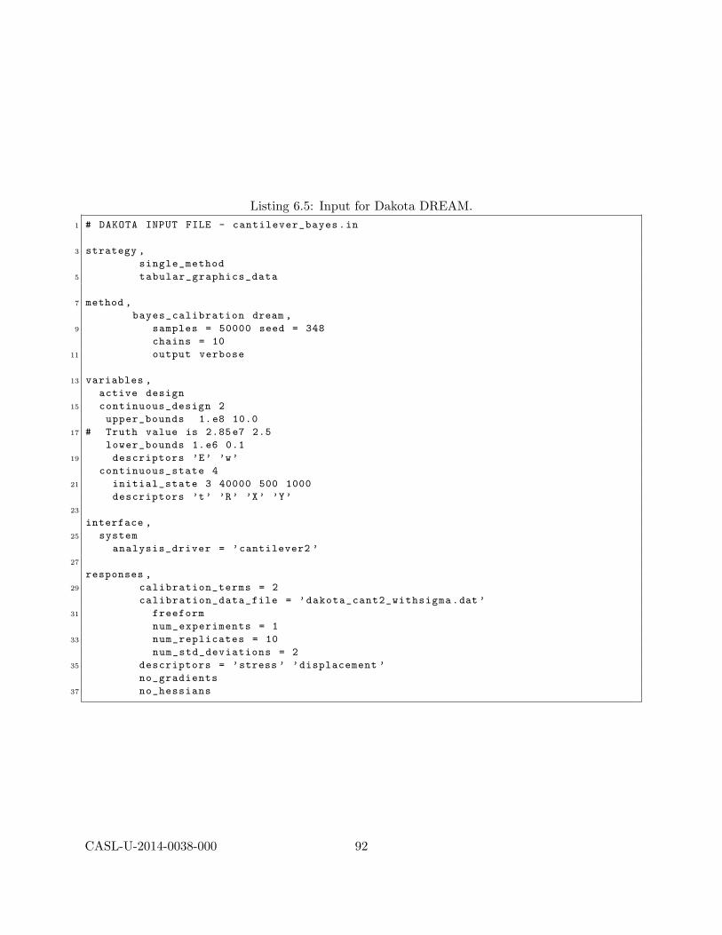
Listing 6.5: Input for Dakota DREAM.1 # DAKOTA INPUT FILE - cantilever_bayes.in
3 strategy ,
single_method
5 tabular_graphics_data
7 method ,
bayes_calibration dream ,
9 samples = 50000 seed = 348
chains = 10
11 output verbose
13 variables ,
active design
15 continuous_design 2
upper_bounds 1.e8 10.0
17 # Truth value is 2.85e7 2.5
lower_bounds 1.e6 0.1
19 descriptors ’E’ ’w’
continuous_state 4
21 initial_state 3 40000 500 1000
descriptors ’t’ ’R’ ’X’ ’Y’
23
interface ,
25 system
analysis_driver = ’cantilever2 ’
27
responses ,
29 calibration_terms = 2
calibration_data_file = ’dakota_cant2_withsigma.dat ’
31 freeform
num_experiments = 1
33 num_replicates = 10
num_std_deviations = 2
35 descriptors = ’stress ’ ’displacement ’
no_gradients
37 no_hessians
CASL-U-2014-0038-000 92

2.82 2.84 2.86 2.88 2.9 2.92
x 107
0
0.5
1
1.5
2
2.5
3
3.5x 10
−6
Stiffness
Direct
DREAM
DRAM
2.49 2.495 2.5 2.505 2.510
20
40
60
80
100
120
Width
Direct
DREAM
DRAM
(a) (b)
Figure 6.5: Marginal posterior densities for (a) E and (b) w generated through direct solution ofBayes’ relation (6.8), Dakota-QUESO DRAM and Dakota DREAM.
2.84 2.86 2.88 2.9 2.92
x 107
2.49
2.495
2.5
2.505
2.51
w
E
DRAM
Figure 6.6: Joint posterior sample points for E and w constructed using the direct method (con-tours) and DRAM (points).
techniques should be employed to determine the set of identifiable or influential parameters. Detailsregarding parameter selection techniques can be found in Chapter 6 of [34].
General Linear Model Verification Tests
We illustrate here aspects of the general linear model verification test suite detailed in Chapter 2and Appendix A. This constitutes step (i) in the verification framework detailed in Section 6.2.4.All results were obtained using the QUESO implementation of DRAM.
CASL-U-2014-0038-000 93

2 2.2 2.4 2.6 2.82.6
2.8
3
3.2
3.4
3.6
Width
Thic
knes
s
2 2.2 2.4 2.6 2.82.8
2.85
2.9
2.95
3
3.05 x 10⁷
Width
Stiff
ness
2.6 2.8 3 3.2 3.4 3.62.8
2.85
2.9
2.95
3
3.05 x 10⁷
Thickness
Stiff
ness
Figure 6.7: Joint posterior sample points for E,w and t using DRAM.
The true values for parameters were constructed using the relations
βi0 = 0.4 + 0.05 sin(
2πi− 1Nβ
), i = 1, . . . , Nβ,
λ0 = 1000, φ0 = 0.3.
The superscript i designates the components of β0.
Example 1. We first generate observations via (2.4) assuming uncorrelated noise, and thencalibrate the unknown variables for several choices of sample size and two separate cases of un-known parameters. This allows verification of convergence of the calibrated variables β and (whereapplicable) λ to their true values. We consider the cases:
• Case 1 (β unknown), Nβ = 1, N ∈ {1, 2, 3, 10, 102, 103, 104, 105, 106},• Case 2 (β, λ unknown), Nβ = 1, N ∈ {2, 3, 10, 102, 103, 104, 105, 106},• Case 1 (β unknown), Nβ = 10, N ∈ {10, 102, 103, 104},• Case 2 (β, λ unknown), Nβ = 10, N ∈ {15, 102, 103, 104}.
Recall that specifying β as unknown is equivalent to stating that β is calibrated to the data. TheNβ = 1 cases were computed using a DRAM chain with 20,000 iterates and the Nβ = 10 cases used50,000 iterates.
CASL-U-2014-0038-000 94

To facilitate visualization for the Nβ = 10 case and provide an intuitive sense of scale, theformulas
βm = 100‖E (β)− β0‖2‖β0‖2 , βv = 100
√var (β)‖β0‖2 ,
λm = 100‖E (λ)− λ0‖2‖λ0‖2 , λv = 100
√var (λ)‖λ0‖2
were used to normalize the results in the plots. Here E(·) denotes the expectation or mean of thechain, var(·) denotes the variance of the chain, and ‖ · ‖2 is the Euclidean norm of the argument.The variables with the m subscript are errors in the expectations of the calibrated variables relativeto true values represented by the variables with subscript 0. The variables with the subscript v arestandard deviations of the chains relative to the magnitude of the true parameters, which providesa more independent sense of the estimated uncertainty. Both of these variables are expressedas percentages and are expected to converge to 0 with increasing sample size for uncorrelatedobservation error. Figure 6.8 illustrates the results of the convergence studies plotted on logarithmicaxes. The downward trend of the plots confirms convergence of the computed quantities to 0 forall considered cases.
We re-emphasize that the results obtained using DRAM are a sequence of iterates drawn froma distribution that characterizes the confidence in the estimate of the unknown parameters. Toillustrate this point, histograms of the iterates obtained for Case 1 (unknown β) assuming a non-informative prior are shown in Figure 6.9 for various sample sizes N . For this problem, the βposterior densities are expected to be Gaussian as confirmed by the shapes of the histograms. Asthe sample size N increases, the mean of the Gaussian posterior density approaches the true param-eter β0 = 0.4 while the variance of the posterior density decreases. A Gaussian density convergesto a Dirac delta distribution (sometimes called an impulse function) as its variance decreases whichFigure 6.9 illustrates. This allows us to conclude that for the case where β is unknown, assigned anoninformative prior, and calibrated to observations corrupted by uncorrelated noise, the estimatefor β tends towards the deterministic value β0 with increasing sample size N . This is consistentwith the intuition that confidence in an estimate increases as the number of data measurementsincreases.
Example 2. Here we compare the posterior densities for the calibrated variables obtained viaDRAM with the exact expressions for the posterior densities computed analytically in Appendix A.For this example, we used a sample size of N = 100 observations generated with equi-correlatederrors, and considered Nβ = 1 regression parameter. We computed the following cases:
• Case 1 (β unknown) with noninformative prior,
• Case 1 (β unknown) with Gaussian prior,
• Case 2 (β, λ unknown) with noninformative prior.
For the Gaussian prior case, we set the mean of the prior to µ0 = 0.6 and the variance to 2× 10⁻⁴.The mean was chosen relatively far from the true value of β0 = 0.4 to distinguish the results fromthose of the noninformative case, thus reducing the possibility of coincidentally correct output. Allcases were computed with parameter chains of 20,000 iterates.
CASL-U-2014-0038-000 95

100 10510−4
10−2
100
102
104
Sample Size N
Rel
ativ
e Er
ror (
%)
` Mean Convergence
Case 1, N`=1
Case 2, N`=1
Case 1, N`=10
Case 2, N`=10
100 105
10−5
100
105
Sample Size N
Frac
tion
of T
rue
(%)
` Standard Deviation Convergence
Case 1, N`=1
Case 2, N`=1
Case 1, N`=10
Case 2, N`=10
(a) (b)
100 105
10−1
100
101
102
Sample Size N
Rel
ativ
e Er
ror (
%)
h Mean Convergence
Case 2, N`=1
Case 2, N`=10
100 105
10−10
10−5
100
105
Sample Size N
Frac
tion
of T
rue h
(%)
h Standard Deviation Convergence
Case 2, N`=1
Case 2, N`=10
(c) (d)
Figure 6.8: Convergence studies for the general linear model verification test suite with uncorrelatednoise and noninformative priors. (a) Percentage error in the mean of β relative to β0. (b) Standarddeviation of β expressed as percentage of β0. (c) Percentage error in mean of λ relative to λ0, and(d) Standard deviation of λ expressed as percentage of λ0.
In Figure 6.10, we show the results for each case. As detailed in Appendix A, Case 1 yields aGaussian posterior density for β whereas the posterior for β in Case 2 is a t-distribution. However,since N = 100 is a moderate sample size (i.e., not small), the t-distribution is roughly Gaussian.The posterior for λ is a Gamma distribution. The DRAM-computed results show good agreementwith the analytic results.
Example 3. Here we compare the analytically computed posterior densities with those obtainedfrom DRAM for small sample sizes (i.e., N ∈ {2, 3, 4, 10}) and an unknown λ to verify thatthe posterior of β matches the expected t-distribution. Both β and λ were calibrated and theparameter chains were computed to 20,000 iterates. We computed the calibration for the threecases of uncorrelated observation errors, equi-correlated observation errors, and AR(1) correlated
CASL-U-2014-0038-000 96
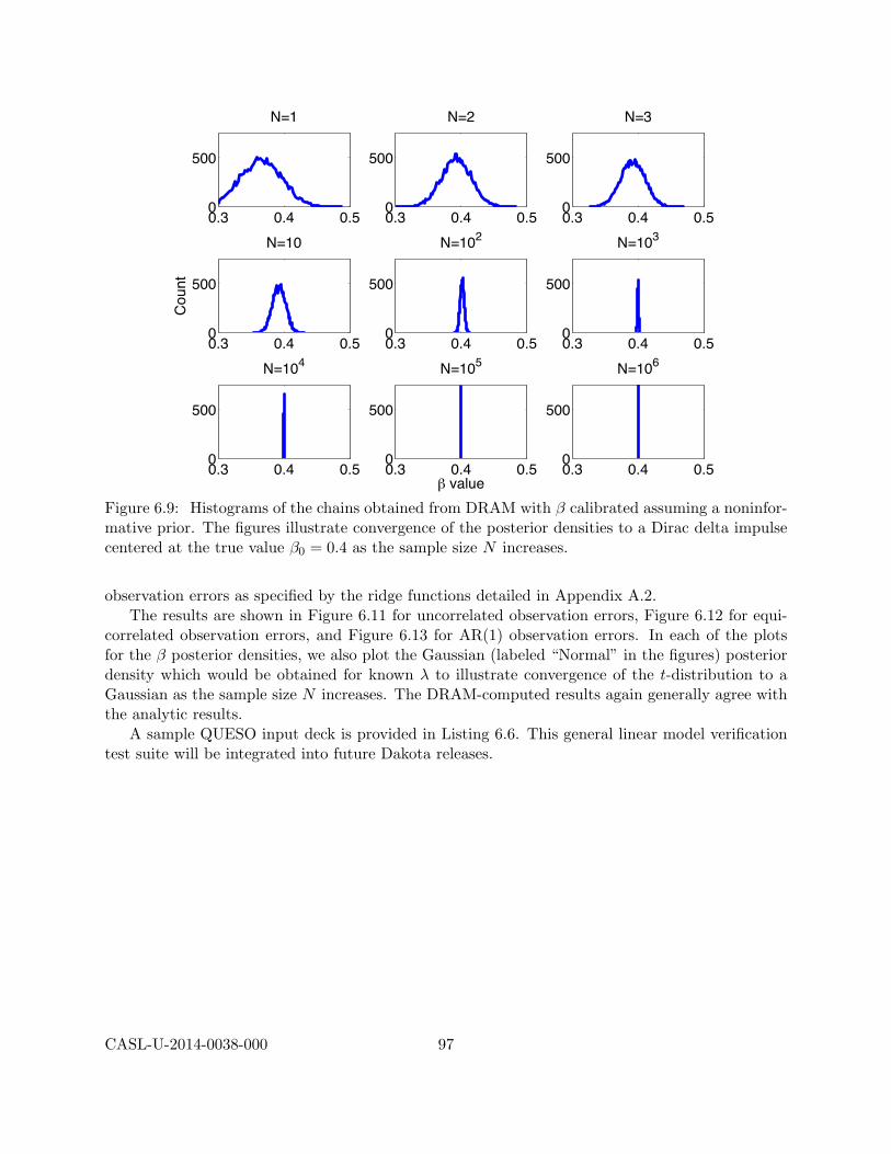
0.3 0.4 0.50
500
N=1
0.3 0.4 0.50
500
N=2
0.3 0.4 0.50
500
N=3
0.3 0.4 0.50
500
Cou
nt
N=10
0.3 0.4 0.50
500
N=102
0.3 0.4 0.50
500
N=103
0.3 0.4 0.50
500
N=104
0.3 0.4 0.50
500
` value
N=105
0.3 0.4 0.50
500
N=106
Figure 6.9: Histograms of the chains obtained from DRAM with β calibrated assuming a noninfor-mative prior. The figures illustrate convergence of the posterior densities to a Dirac delta impulsecentered at the true value β0 = 0.4 as the sample size N increases.
observation errors as specified by the ridge functions detailed in Appendix A.2.The results are shown in Figure 6.11 for uncorrelated observation errors, Figure 6.12 for equi-
correlated observation errors, and Figure 6.13 for AR(1) observation errors. In each of the plotsfor the β posterior densities, we also plot the Gaussian (labeled “Normal” in the figures) posteriordensity which would be obtained for known λ to illustrate convergence of the t-distribution to aGaussian as the sample size N increases. The DRAM-computed results again generally agree withthe analytic results.
A sample QUESO input deck is provided in Listing 6.6. This general linear model verificationtest suite will be integrated into future Dakota releases.
CASL-U-2014-0038-000 97

0.34 0.36 0.38 0.4 0.42 0.44 0.460
5
10
15
20
25
Prob
abilit
y
`
`, Case 1, Non−informative Prior
DRAMAnalytic
0.48 0.5 0.52 0.54 0.560
5
10
15
20
25
30
35
40
Prob
abilit
y`
`, Case 1, Gaussian Prior
DRAMAnalytic
(a) (b)
0.35 0.4 0.450
5
10
15
20
25
Prob
abilit
y
`
`, Case 2, Non−informative Prior
DRAMAnalytic
500 1000 15000
0.5
1
1.5
2
2.5
3
3.5 x 10⁻³
Prob
abilit
y
h
h, Case 2, Non−informative Prior
DRAMAnalytic
(c) (d)
Figure 6.10: Comparison of DRAM-computed posterior densities for β, λ with the analytic posteriordensities. Case 1: β posterior density with β unknown assuming a (a) noninformative prior and(b) Gaussian prior. Case 2: β, λ unknown, calibrated assuming a noninformative prior, and theresulting (c) β posterior density and (d) λ posterior density.
CASL-U-2014-0038-000 98
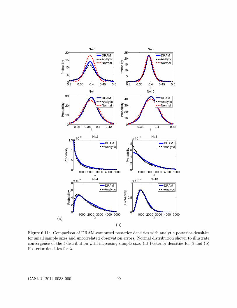
0.3 0.35 0.4 0.45 0.50
5
10
15
20N=2
`
Prob
abilit
y
DRAMAnalyticNormal
0.3 0.35 0.4 0.45 0.50
5
10
15
20
25N=3
`
Prob
abilit
y
DRAMAnalyticNormal
0.36 0.38 0.4 0.420
10
20
30N=4
`
Prob
abilit
y
DRAMAnalyticNormal
0.38 0.4 0.420
10
20
30
40
N=10
`
Prob
abilit
y
DRAMAnalyticNormal
(a)
1000 2000 3000 4000 50000
0.5
1
1.5x 10
−3 N=2
λ
Pro
ba
bili
ty
DRAM
Analytic
1000 2000 3000 4000 50000
2
4
6
8
x 10−4 N=3
λ
Pro
ba
bili
ty
DRAM
Analytic
1000 2000 3000 4000 50000
2
4
6
8x 10
−4 N=4
λ
Pro
ba
bili
ty
DRAM
Analytic
1000 2000 3000 4000 50000
0.5
1x 10
−3 N=10
λ
Pro
ba
bili
ty
DRAM
Analytic
(b)
Figure 6.11: Comparison of DRAM-computed posterior densities with analytic posterior densitiesfor small sample sizes and uncorrelated observation errors. Normal distribution shown to illustrateconvergence of the t-distribution with increasing sample size. (a) Posterior densities for β and (b)Posterior densities for λ.
CASL-U-2014-0038-000 99
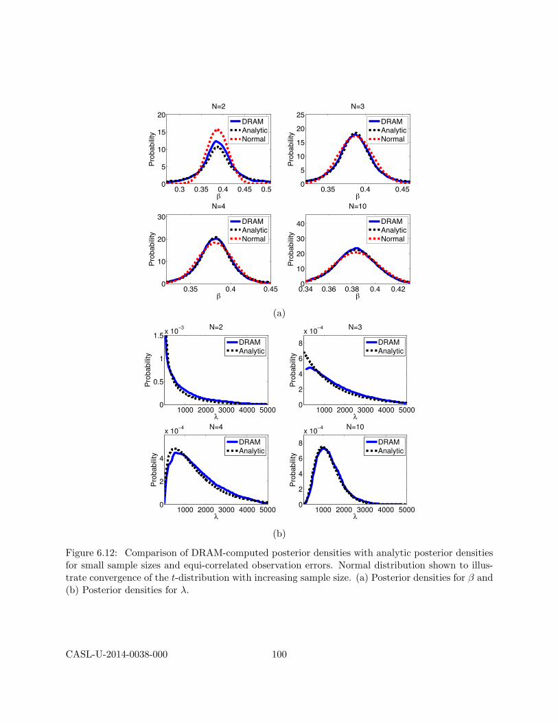
0.3 0.35 0.4 0.45 0.50
5
10
15
20N=2
`
Prob
abilit
y
DRAMAnalyticNormal
0.35 0.4 0.450
5
10
15
20
25N=3
`
Prob
abilit
y
DRAMAnalyticNormal
0.35 0.4 0.450
10
20
30N=4
`
Prob
abilit
y
DRAMAnalyticNormal
0.34 0.36 0.38 0.4 0.420
10
20
30
40
N=10
`Pr
obab
ility
DRAMAnalyticNormal
(a)
1000 2000 3000 4000 50000
0.5
1
1.5x 10
−3 N=2
λ
Pro
ba
bili
ty
DRAM
Analytic
1000 2000 3000 4000 50000
2
4
6
8
x 10−4 N=3
λ
Pro
ba
bili
ty
DRAM
Analytic
1000 2000 3000 4000 50000
2
4
x 10−4 N=4
λ
Pro
ba
bili
ty
DRAM
Analytic
1000 2000 3000 4000 50000
2
4
6
8
x 10−4 N=10
λ
Pro
ba
bili
ty
DRAM
Analytic
(b)
Figure 6.12: Comparison of DRAM-computed posterior densities with analytic posterior densitiesfor small sample sizes and equi-correlated observation errors. Normal distribution shown to illus-trate convergence of the t-distribution with increasing sample size. (a) Posterior densities for β and(b) Posterior densities for λ.
CASL-U-2014-0038-000 100
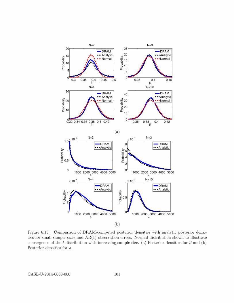
0.3 0.35 0.4 0.45 0.50
5
10
15
20N=2
`
Prob
abilit
y
DRAMAnalyticNormal
0.35 0.4 0.450
5
10
15
20
25N=3
`
Prob
abilit
y
DRAMAnalyticNormal
0.32 0.34 0.36 0.38 0.4 0.420
10
20
30N=4
`
Prob
abilit
y
DRAMAnalyticNormal
0.36 0.38 0.4 0.420
10
20
30
40
N=10
`Pr
obab
ility
DRAMAnalyticNormal
(a)
1000 2000 3000 4000 50000
0.5
1
1.5x 10
−3 N=2
λ
Pro
ba
bili
ty
DRAM
Analytic
1000 2000 3000 4000 50000
2
4
6
8
x 10−4 N=3
λ
Pro
ba
bili
ty
DRAM
Analytic
1000 2000 3000 4000 50000
2
4
x 10−4 N=4
λ
Pro
ba
bili
ty
DRAM
Analytic
1000 2000 3000 4000 50000
0.5
1x 10
−3 N=10
λ
Pro
ba
bili
ty
DRAM
Analytic
(b)
Figure 6.13: Comparison of DRAM-computed posterior densities with analytic posterior densi-ties for small sample sizes and AR(1) observation errors. Normal distribution shown to illustrateconvergence of the t-distribution with increasing sample size. (a) Posterior densities for β and (b)Posterior densities for λ.
CASL-U-2014-0038-000 101

Listing 6.6: QUESO input for the general linear model verification test suite.###############################################
2 # UQ Environment
###############################################
4 env_numSubEnvironments = 1
env_subDisplayFileName = outputData/display_env
6 env_subDisplayAllowAll = 0
env_subDisplayAllowedSet = 0 1 2 3 4 5 6 7
8 env_displayVerbosity = 2
env_seed = 0
10
###############################################
12 # Statistical inverse problem (ip)
###############################################
14 ip_computeSolution = 1
ip_dataOutputFileName = outputData/sip_algver
16 ip_dataOutputAllowedSet = 0 1
18 ###############################################
# Information for Metropolis -Hastings algorithm
20 ###############################################
ip_mh_dataOutputFileName = outputData/sip_algver
22 ip_mh_dataOutputAllowedSet = 0 1
24 ip_mh_rawChain_dataInputFileName = .
ip_mh_rawChain_size = 20000
26 ip_mh_rawChain_generateExtra = 0
ip_mh_rawChain_displayPeriod = 2000
28 ip_mh_rawChain_measureRunTimes = 1
ip_mh_rawChain_dataOutputFileName = outputData/sip_algver_raw_chain
30 ip_mh_rawChain_dataOutputAllowedSet = 0 1 2 3 4 5 6 7
32 ip_mh_displayCandidates = 0
ip_mh_putOutOfBoundsInChain = 0
34 ip_mh_dr_maxNumExtraStages = 3
ip_mh_dr_listOfScalesForExtraStages = 5. 10. 20.
36 ip_mh_am_initialNonAdaptInterval = 0
ip_mh_am_adaptInterval = 200
38 ip_mh_am_eta = 0.05703 #(2.4^2)/d, d is
the dimension of the problem
40 ip_mh_am_epsilon = 1.e-5
42 ip_mh_filteredChain_generate = 1
ip_mh_filteredChain_discardedPortion = 0.
44 ip_mh_filteredChain_lag = 10
ip_mh_filteredChain_dataOutputFileName = outputData/sip_algver_filtered_chain
46 ip_mh_filteredChain_dataOutputAllowedSet = 0 1
CASL-U-2014-0038-000 102
Chapter 7
COBRA-TF VUQ Studies
This chapter concludes the manual by demonstrating use of Dakota to complete an overall VUQprocess for CASL Progression Problem 6, simulated with COBRA-TF, as described in Section 2.3.The workflow demonstration includes the following Dakota studies:
1. Initial centered parameter studies to exercise the COBRA-TF model with two coupledphysics scenarios and verify the Dakota/COBRA-TF interfaces, resulting in adding and re-moving some parameters from the admissible set. (Section 7.1)
2. Sensitivity analysis using parameter study, LHS and Morris methods to identify the mostimportant of 33 parameters. Initial LHS studies revealed code robustness issues under jointvariation, resulting in adjusting the range of one parameter. Screening based on these studiesresulted in five significant parameters. Another LHS study with 50 samples was conductedover these parameters and used in subsequent activities. (Section 7.2)
3. Deterministic and Bayesian calibration to estimate the values or distributions of thefive significant parameters using synthetic data. The deterministic calibration demonstratesgradient-based local calibration using the COBRA-TF simulation model directly, while theBayesian calibration uses a surrogate model constructed from the 50 LHS samples. (Sec-tion 7.3)
4. Surrogate construction and validation to assess the quality and applicability of a responsesurface model. (Section 7.3.2)
The total Progression Problem 6 parameter set for consideration is indicated in Table 2.6 inSection 2.3. The two parameters marked with an asterisk in this table, ql and qv, were initiallyincluded to assess the effects of heat transfer across the fuel pin surface into the channel liquid andvapor phases, respectively. However, it was quickly discovered that for the steady-state ProgressionProblem 6, perturbing either of these produces an inherent thermal imbalance precluding any steadythermal behavior. Accordingly, these parameters were excluded from the following studies. For allstudies in this chapter, the total pressure drop through the fuel rod assembly (here indicated byTotalPressure) was used as the quantity of interest.
CASL-U-2014-0038-000 103

7.1 Initial Parameter Studies with Two Power Distributions
Two initial centered parameter studies were conducted to verify the Dakota/COBRA-TF interface,assess code robustness, and generate initial results. Both employed a Dakota centered parameterstudy (Section 3.2.1) over 29 parameters for which the shift values were zero, e.g. kap = 0, and thescaling values were allowed to vary by ±5% around unity, e.g. kp = 1.0± 5% in increments of 1%.The two studies differ in the power distribution input to the thermal hydraulics code. The firstuses a uniform value specified via input, while the second uses an axially varying power distribu-tion representing a converged steady-state solution from a previous full simulation of ProgressionProblem 6. The second study represents a parameter sensitivity study performed around the actualsolution to the neutronics component of the problem. The four parameters k xkwlx, k cd, k cdfb,and k wkr were not yet available in the Dakota/COBRA-TF interface when these early studieswere conducted.
The initial centered parameter studies each involve 29 parameters evaluated at 10 pertubedvalues in addition to the baseline (nominal) evaluation. This amounts to 291 total runs for eachstudy. Dakota provides a concurrent execution facility which for these studies enables 60 indepen-dent runs to execute simultaneously on the james007 CASL machine. Each run requires between5 and 7 minutes so that each centered parameter study completes in just under 1 hour assumingavailable capacity on the machine.
Table 7.1 summarizes the results for the uniform power distribution, and Table 7.2 summarizesresults for the spatially varying power distribution. All values are reported as percentages of thedifference in total pressure drop across the fuel assembly compared to a baseline value representingunperturbed parameter values. All parameters were perturbed in the same manner, e.g. the scalingcoefficient was adjusted -5% to +5% in increments of 1%. The inlet mass flow rate finlet wasincorrectly included in these initial studies and later removed in the final study when the axial wallfriction and the three loss coefficients for grid spacers were added. These initial results demonstratethe iterative exploratory process of conducting Dakota studies on models, so detailed discussion isomitted.
7.2 COBRA-TF Sensitivity Studies
Initial studies helped stabilize the admissible parameter set to 33 key parameters, for which the VUQprocess is demonstrated in this section. The first step in sensitivity analysis is to perform a centeredparameter study to assess the effect of individual parameters on the simulation response. Thenwe conduct Dakota analyses that jointly vary the parameters to better assess global sensitvitiesfor complex models. The Latin hypercube and Morris methods complement the parameter studyresults to screen the parameter set.
7.2.1 Centered Parameter Study
Dakota Input: A Dakota input file dakota centered 33.in for a 33 variable (now including pa-rameters k xkwlx, k cd, k cdfb, and k wkr) centered parameter study is shown in Listing 7.1. Themethod section (line 6) prescribes the study with five each positive and negative parameter steps of0.01. The 33 COBRA-TF parameters are specified in the variables section, with an initial pointof 1.0 (line 14), indicating nominal input values for the simulation. The interface (line 17) speci-fies use of the dakota-vera-analysis driver (line 21), which implements the Dakota/COBRA-TF
CASL-U-2014-0038-000 104
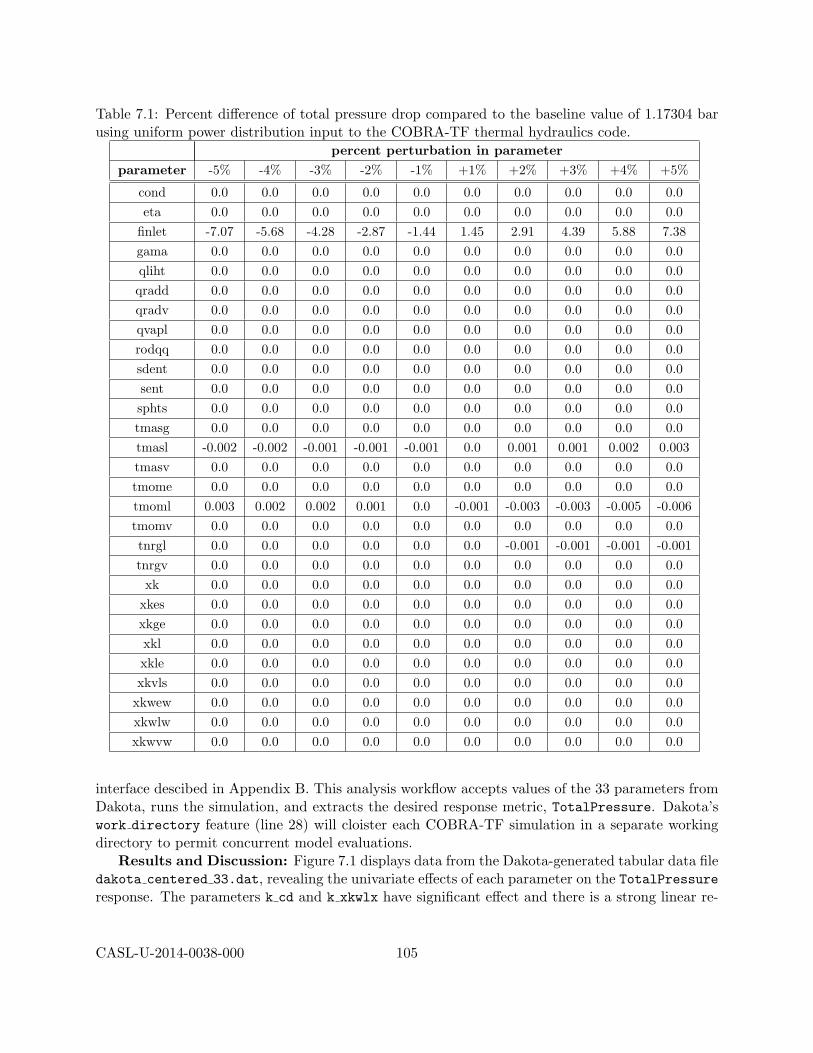
Table 7.1: Percent difference of total pressure drop compared to the baseline value of 1.17304 barusing uniform power distribution input to the COBRA-TF thermal hydraulics code.
percent perturbation in parameterparameter -5% -4% -3% -2% -1% +1% +2% +3% +4% +5%
cond 0.0 0.0 0.0 0.0 0.0 0.0 0.0 0.0 0.0 0.0eta 0.0 0.0 0.0 0.0 0.0 0.0 0.0 0.0 0.0 0.0
finlet -7.07 -5.68 -4.28 -2.87 -1.44 1.45 2.91 4.39 5.88 7.38gama 0.0 0.0 0.0 0.0 0.0 0.0 0.0 0.0 0.0 0.0qliht 0.0 0.0 0.0 0.0 0.0 0.0 0.0 0.0 0.0 0.0qradd 0.0 0.0 0.0 0.0 0.0 0.0 0.0 0.0 0.0 0.0qradv 0.0 0.0 0.0 0.0 0.0 0.0 0.0 0.0 0.0 0.0qvapl 0.0 0.0 0.0 0.0 0.0 0.0 0.0 0.0 0.0 0.0rodqq 0.0 0.0 0.0 0.0 0.0 0.0 0.0 0.0 0.0 0.0sdent 0.0 0.0 0.0 0.0 0.0 0.0 0.0 0.0 0.0 0.0sent 0.0 0.0 0.0 0.0 0.0 0.0 0.0 0.0 0.0 0.0sphts 0.0 0.0 0.0 0.0 0.0 0.0 0.0 0.0 0.0 0.0tmasg 0.0 0.0 0.0 0.0 0.0 0.0 0.0 0.0 0.0 0.0tmasl -0.002 -0.002 -0.001 -0.001 -0.001 0.0 0.001 0.001 0.002 0.003tmasv 0.0 0.0 0.0 0.0 0.0 0.0 0.0 0.0 0.0 0.0tmome 0.0 0.0 0.0 0.0 0.0 0.0 0.0 0.0 0.0 0.0tmoml 0.003 0.002 0.002 0.001 0.0 -0.001 -0.003 -0.003 -0.005 -0.006tmomv 0.0 0.0 0.0 0.0 0.0 0.0 0.0 0.0 0.0 0.0tnrgl 0.0 0.0 0.0 0.0 0.0 0.0 -0.001 -0.001 -0.001 -0.001tnrgv 0.0 0.0 0.0 0.0 0.0 0.0 0.0 0.0 0.0 0.0
xk 0.0 0.0 0.0 0.0 0.0 0.0 0.0 0.0 0.0 0.0xkes 0.0 0.0 0.0 0.0 0.0 0.0 0.0 0.0 0.0 0.0xkge 0.0 0.0 0.0 0.0 0.0 0.0 0.0 0.0 0.0 0.0xkl 0.0 0.0 0.0 0.0 0.0 0.0 0.0 0.0 0.0 0.0xkle 0.0 0.0 0.0 0.0 0.0 0.0 0.0 0.0 0.0 0.0xkvls 0.0 0.0 0.0 0.0 0.0 0.0 0.0 0.0 0.0 0.0
xkwew 0.0 0.0 0.0 0.0 0.0 0.0 0.0 0.0 0.0 0.0xkwlw 0.0 0.0 0.0 0.0 0.0 0.0 0.0 0.0 0.0 0.0xkwvw 0.0 0.0 0.0 0.0 0.0 0.0 0.0 0.0 0.0 0.0
interface descibed in Appendix B. This analysis workflow accepts values of the 33 parameters fromDakota, runs the simulation, and extracts the desired response metric, TotalPressure. Dakota’swork directory feature (line 28) will cloister each COBRA-TF simulation in a separate workingdirectory to permit concurrent model evaluations.
Results and Discussion: Figure 7.1 displays data from the Dakota-generated tabular data filedakota centered 33.dat, revealing the univariate effects of each parameter on the TotalPressureresponse. The parameters k cd and k xkwlx have significant effect and there is a strong linear re-
CASL-U-2014-0038-000 105
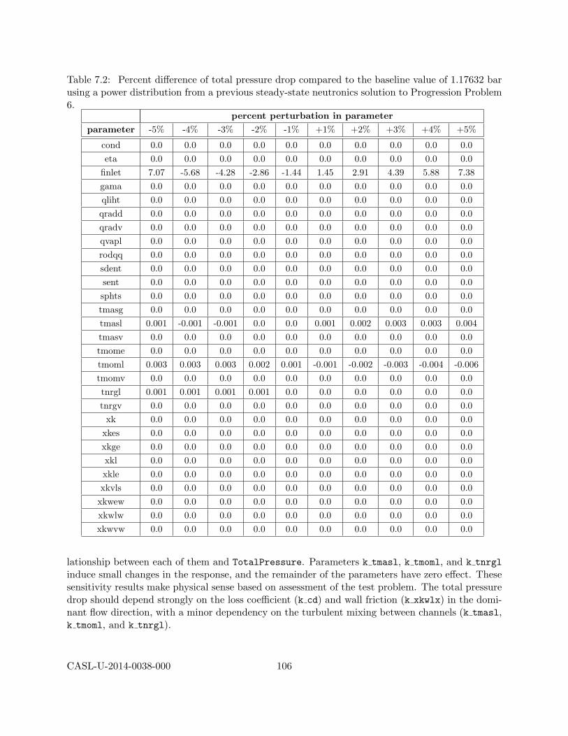
Table 7.2: Percent difference of total pressure drop compared to the baseline value of 1.17632 barusing a power distribution from a previous steady-state neutronics solution to Progression Problem6.
percent perturbation in parameterparameter -5% -4% -3% -2% -1% +1% +2% +3% +4% +5%
cond 0.0 0.0 0.0 0.0 0.0 0.0 0.0 0.0 0.0 0.0eta 0.0 0.0 0.0 0.0 0.0 0.0 0.0 0.0 0.0 0.0
finlet 7.07 -5.68 -4.28 -2.86 -1.44 1.45 2.91 4.39 5.88 7.38gama 0.0 0.0 0.0 0.0 0.0 0.0 0.0 0.0 0.0 0.0qliht 0.0 0.0 0.0 0.0 0.0 0.0 0.0 0.0 0.0 0.0qradd 0.0 0.0 0.0 0.0 0.0 0.0 0.0 0.0 0.0 0.0qradv 0.0 0.0 0.0 0.0 0.0 0.0 0.0 0.0 0.0 0.0qvapl 0.0 0.0 0.0 0.0 0.0 0.0 0.0 0.0 0.0 0.0rodqq 0.0 0.0 0.0 0.0 0.0 0.0 0.0 0.0 0.0 0.0sdent 0.0 0.0 0.0 0.0 0.0 0.0 0.0 0.0 0.0 0.0sent 0.0 0.0 0.0 0.0 0.0 0.0 0.0 0.0 0.0 0.0sphts 0.0 0.0 0.0 0.0 0.0 0.0 0.0 0.0 0.0 0.0tmasg 0.0 0.0 0.0 0.0 0.0 0.0 0.0 0.0 0.0 0.0tmasl 0.001 -0.001 -0.001 0.0 0.0 0.001 0.002 0.003 0.003 0.004tmasv 0.0 0.0 0.0 0.0 0.0 0.0 0.0 0.0 0.0 0.0tmome 0.0 0.0 0.0 0.0 0.0 0.0 0.0 0.0 0.0 0.0tmoml 0.003 0.003 0.003 0.002 0.001 -0.001 -0.002 -0.003 -0.004 -0.006tmomv 0.0 0.0 0.0 0.0 0.0 0.0 0.0 0.0 0.0 0.0tnrgl 0.001 0.001 0.001 0.001 0.0 0.0 0.0 0.0 0.0 0.0tnrgv 0.0 0.0 0.0 0.0 0.0 0.0 0.0 0.0 0.0 0.0
xk 0.0 0.0 0.0 0.0 0.0 0.0 0.0 0.0 0.0 0.0xkes 0.0 0.0 0.0 0.0 0.0 0.0 0.0 0.0 0.0 0.0xkge 0.0 0.0 0.0 0.0 0.0 0.0 0.0 0.0 0.0 0.0xkl 0.0 0.0 0.0 0.0 0.0 0.0 0.0 0.0 0.0 0.0xkle 0.0 0.0 0.0 0.0 0.0 0.0 0.0 0.0 0.0 0.0xkvls 0.0 0.0 0.0 0.0 0.0 0.0 0.0 0.0 0.0 0.0
xkwew 0.0 0.0 0.0 0.0 0.0 0.0 0.0 0.0 0.0 0.0xkwlw 0.0 0.0 0.0 0.0 0.0 0.0 0.0 0.0 0.0 0.0xkwvw 0.0 0.0 0.0 0.0 0.0 0.0 0.0 0.0 0.0 0.0
lationship between each of them and TotalPressure. Parameters k tmasl, k tmoml, and k tnrglinduce small changes in the response, and the remainder of the parameters have zero effect. Thesesensitivity results make physical sense based on assessment of the test problem. The total pressuredrop should depend strongly on the loss coefficient (k cd) and wall friction (k xkwlx) in the domi-nant flow direction, with a minor dependency on the turbulent mixing between channels (k tmasl,k tmoml, and k tnrgl).
CASL-U-2014-0038-000 106

Listing 7.1: Dakota input file for centered parameter study, with ±5% variation in each of 33parameters.
1 strategy
single_method
3 tabular_graphics_data
tabular_graphics_file ’dakota_centered_33.dat ’
5
method
7 # 11 total evaluations over range [0.95 ,1.05]
centered_parameter_study
9 step_vector 0.01 0.01 0.01 0.01 0.01 0.01 0.01 0.01 0.01 0.01 0.01 0.01 0.01
0.01 0.01 0.01 0.01 0.01 0.01 0.01 0.01 0.01 0.01 0.01 0.01 0.01 0.01 0.01
0.01 0.01 0.01 0.01 0.01
steps_per_variable 5
11
variables
13 continuous_design 33
initial_point 1.0 1.0 1.0 1.0 1.0 1.0 1.0 1.0 1.0 1.0 1.0 1.0 1.0 1.0
1.0 1.0 1.0 1.0 1.0 1.0 1.0 1.0 1.0 1.0 1.0 1.0 1.0 1.0 1.0 1.0 1.0 1.0 1.0
15 descriptors ’k_eta ’ ’k_gama ’ ’k_sent ’ ’k_sdent ’ ’k_tmasv ’ ’k_tmasl ’ ’
k_tmasg ’ ’k_tmomv ’ ’k_tmome ’ ’k_tmoml ’ ’k_xk ’ ’k_xkes ’ ’k_xkge ’ ’k_xkl ’ ’
k_xkle ’ ’k_xkvls ’ ’k_xkwvw ’ ’k_xkwlw ’ ’k_xkwew ’ ’k_qvapl ’ ’k_tnrgv ’ ’k_tnrgl ’
’k_rodqq ’ ’k_qradd ’ ’k_qradv ’ ’k_qliht ’ ’k_sphts ’ ’k_cond ’ ’k_xkwvx ’ ’
k_xkwlx ’ ’k_cd ’ ’k_cdfb ’ ’k_wkr ’
17 interface
fork
19 asynchronous
evaluation_concurrency = 60
21 analysis_driver = ’dakota -vera -analysis ’
# extract TotalPressure metric (length 1)
23 analysis_components = ’TotPress ’
parameters_file = ’params.in ’
25 # aprepro
results_file = ’results.out ’
27 failure_capture recover NaN
work_directory
29 directory_tag
named ’workdir ’
31 file_save directory_save
33 responses
num_response_functions = 1
35 descriptors
’TotalPressure ’
37 no_gradients
no_hessians
CASL-U-2014-0038-000 107
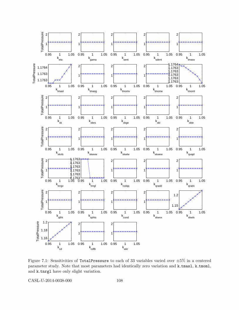
0.95 1 1.05
1
2
keta
Tot
alP
ress
ure
0.95 1 1.05
1
2
kgama
0.95 1 1.05
1
2
ksent
0.95 1 1.05
1
2
ksdent
0.95 1 1.05
1
2
ktmasv
0.95 1 1.05
1.1763
1.1763
1.1764
ktmasl
Tot
alP
ress
ure
0.95 1 1.05
1
2
ktmasg
0.95 1 1.05
1
2
ktmomv
0.95 1 1.05
1
2
ktmome
0.95 1 1.051.17631.17631.17631.17631.17631.1764
ktmoml
0.95 1 1.05
1
2
kxk
Tot
alP
ress
ure
0.95 1 1.05
1
2
kxkes
0.95 1 1.05
1
2
kxkge
0.95 1 1.05
1
2
kxkl
0.95 1 1.05
1
2
kxkle
0.95 1 1.05
1
2
kxkvls
Tot
alP
ress
ure
0.95 1 1.05
1
2
kxkwvw
0.95 1 1.05
1
2
kxkwlw
0.95 1 1.05
1
2
kxkwew
0.95 1 1.05
1
2
kqvapl
0.95 1 1.05
1
2
ktnrgv
Tot
alP
ress
ure
0.95 1 1.051.17631.17631.17631.17631.17631.1763
ktnrgl
0.95 1 1.05
1
2
krodqq
0.95 1 1.05
1
2
kqradd
0.95 1 1.05
1
2
kqradv
0.95 1 1.05
1
2
kqliht
Tot
alP
ress
ure
0.95 1 1.05
1
2
ksphts
0.95 1 1.05
1
2
kcond
0.95 1 1.05
1
2
kxkwvx
0.95 1 1.05
1.15
1.2
kxkwlx
0.95 1 1.05
1.16
1.18
1.2
kcd
Tot
alP
ress
ure
0.95 1 1.05
1
2
kcdfb
0.95 1 1.05
1
2
kwkr
Figure 7.1: Sensitivities of TotalPressure to each of 33 variables varied over ±5% in a centeredparameter study. Note that most parameters had identically zero variation and k tmasl, k tmoml,and k tnrgl have only slight variation.
CASL-U-2014-0038-000 108

7.2.2 Latin hypercube sampling studies
Latin hypercube sampling for sensitivity analysis is described in Section 3.2.3. Since all theCOBRA-TF parameters affect model form in the solution, they are taken to have uniform dis-tributions on the interval [−10%, 10%]. Upon conducting initial LHS studies, the simulation failedto converge when run with deviation of k tmasl > 5%. Two possibilities for this failure are likelyand would require additional investigation to fully diagnose. One possibility is that perturbing thisparameter along with others pertinent to overall mass conservation introduces an inherent incon-sistency precluding steady mass conservation. Another possibility involves the temporal stabilityof running COBRA-TF to a steady state. Increasing k tmasl too much may violate the stabilityrequirements of the COBRA-TF time integration method such that a steady-state is not reached.We did not pursue this further but instead decreased the range of perturbation of this parametersuch that converged steady-state solutions were obtained in a stable manner. Therefore a uniformdistribution on [−5%, 5%] was used for this parameter.
Dakota Input: To change the Dakota input from a centered parameter study to a LHSstudy, the method and variables specifications change. The method block now prescribes a Latinhypercube sampling study. The number of samples is specified to be N = 10×(M =) 33 parameters,or N = 330:
methodsamplingsample_type lhssamples = 330seed = 52983
The variables section changes to use uncertain variables with a uniform distribution on [0.9, 1.1],except for k tmasl ∈ [0.95, 1.05]:
uniform_uncertain = 33upper_bounds 1.1 1.1 1.1 1.1 1.1 1.05 1.1 1.1 1.1 1.1 1.1 1.1 1.1
1.1 1.1 1.1 1.1 1.1 1.1 1.1 1.1 1.1 1.1 1.1 1.1 1.11.1 1.1 1.1 1.1 1.1 1.1 1.1
lower_bounds 0.9 0.9 0.9 0.9 0.9 0.95 0.9 0.9 0.9 0.9 0.9 0.9 0.90.9 0.9 0.9 0.9 0.9 0.9 0.9 0.9 0.9 0.9 0.9 0.9 0.90.9 0.9 0.9 0.9 0.9 0.9 0.9
The full Dakota input file dakota lhs 33.in is shown in Listing 7.2.Results and Discussion: Relevant outputs generated by Dakota include the correlation coef-
ficients in the screen output dakota lhs 33.out, and tabulated data in dakota lhs 33.dat. Theportion of the Dakota console output with the partial correlation coefficients is shown in Fig-ure 7.2. The output is easier to comprehend when plotted with Matlab, as shown in the bar graphin Figure 7.3. The partial correlation coefficients near 1.0 indicate that there is a strong linear cor-relation between k cd and TotalPressure and between k xkwlx and TotalPressure, consistentwith physical intuition that total pressure drop should depend linearly on both the axial grid spacerloss coefficient and the axial wall friction coefficient. No other parameters are strongly significantby this measure (greater than 0.5), although several are greater than 0.1 and could be consideredfor inclusion in follow-on analyses based on assessment of their interaction with other parametersor nonlinear behavior.
CASL-U-2014-0038-000 109

Listing 7.2: Dakota input file for Latin hypercube sampling-based sensitivity analysis study with330 samples and uniform input distributions.strategy
2 single_method
tabular_graphics_data
4 tabular_graphics_file ’dakota_lhs_33.dat ’
6 method
sampling
8 sample_type lhs
samples = 330
10 seed = 52983
12 variables
uniform_uncertain = 33
14 upper_bounds 1.1 1.1 1.1 1.1 1.1 1.05 1.1 1.1 1.1 1.1 1.1 1.1 1.1 1.1
1.1 1.1 1.1 1.1 1.1 1.1 1.1 1.1 1.1 1.1 1.1 1.1 1.1 1.1 1.1 1.1 1.1 1.1 1.1
lower_bounds 0.9 0.9 0.9 0.9 0.9 0.95 0.9 0.9 0.9 0.9 0.9 0.9 0.9 0.9
0.9 0.9 0.9 0.9 0.9 0.9 0.9 0.9 0.9 0.9 0.9 0.9 0.9 0.9 0.9 0.9 0.9 0.9 0.9
16 descriptors ’k_eta ’ ’k_gama ’ ’k_sent ’ ’k_sdent ’ ’k_tmasv ’ ’k_tmasl ’ ’
k_tmasg ’ ’k_tmomv ’ ’k_tmome ’ ’k_tmoml ’ ’k_xk ’ ’k_xkes ’ ’k_xkge ’ ’k_xkl ’ ’
k_xkle ’ ’k_xkvls ’ ’k_xkwvw ’ ’k_xkwlw ’ ’k_xkwew ’ ’k_qvapl ’ ’k_tnrgv ’ ’k_tnrgl ’
’k_rodqq ’ ’k_qradd ’ ’k_qradv ’ ’k_qliht ’ ’k_sphts ’ ’k_cond ’ ’k_xkwvx ’ ’
k_xkwlx ’ ’k_cd ’ ’k_cdfb ’ ’k_wkr ’
18 interface
fork
20 asynchronous
evaluation_concurrency = 60
22 analysis_driver = ’dakota -vera -analysis ’
# extract TotalPressure metric (length 1)
24 analysis_components = ’TotPress ’
parameters_file = ’params.in ’
26 # aprepro
results_file = ’results.out ’
28 failure_capture recover NaN
work_directory
30 directory_tag
named ’workdir ’
32 file_save directory_save
34 responses
num_response_functions = 1
36 descriptors
’TotalPressure ’
38 no_gradients
no_hessians
CASL-U-2014-0038-000 110

Partial Correlation Matrix between input and output:TotalPressure
k_eta 7.48866e-02k_gama -3.07977e-02k_sent -3.36640e-02k_sdent -6.83465e-02k_tmasv -3.48366e-02k_tmasl 1.11817e-01k_tmasg -1.88872e-01k_tmomv -1.15407e-01k_tmome 1.68634e-02k_tmoml 1.90197e-02
k_xk 8.00607e-02k_xkes -4.52322e-02k_xkge -6.88362e-02k_xkl 3.59859e-02
k_xkle -3.31872e-02k_xkvls 1.08367e-01k_xkwvw -9.66830e-02k_xkwlw 1.43162e-01k_xkwew -7.26037e-03k_qvapl -8.55824e-02k_tnrgv -2.87188e-02k_tnrgl -5.43819e-03k_rodqq 1.81288e-02k_qradd -2.23918e-02k_qradv -1.10458e-02k_qliht -8.77747e-03k_sphts -4.76993e-02k_cond -3.93625e-02k_xkwvx 3.31933e-02k_xkwlx 9.99585e-01
k_cd 9.98520e-01k_cdfb -1.86595e-02k_wkr 2.35471e-02
Figure 7.2: Dakota console output showing partial correlations for the COBRA-TF simulatedProgression Problem 6.
CASL-U-2014-0038-000 111

−0.5 0 0.5 1 1.5
k_{eta}k_{gama}
k_{sent}k_{sdent}k_{tmasv}k_{tmasl}
k_{tmasg}k_{tmomv}k_{tmome}k_{tmoml}
k_{xk}k_{xkes}k_{xkge}
k_{xkl}k_{xkle}
k_{xkvls}k_{xkwvw}k_{xkwlw}
k_{xkwew}k_{qvapl}k_{tnrgv}k_{tnrgl}
k_{rodqq}k_{qradd}k_{qradv}
k_{qliht}k_{sphts}k_{cond}
k_{xkwvx}k_{xkwlx}
k_{cd}k_{cdfb}k_{wkr}
0.07
−0.03
−0.03
−0.07
−0.03
0.11
−0.19
−0.12
0.02
0.02
0.08
−0.05
−0.07
0.04
−0.03
0.11
−0.10
0.14
−0.01
−0.09
−0.03
−0.01
0.02
−0.02
−0.01
−0.01
−0.05
−0.04
0.03
1.00
1.00
−0.02
0.02
Partial correlation for TotalPressure
Figure 7.3: Bar graph showing partial correlation for each of 33 variables with TotalPressure forthe COBRA-TF simulated Progression Problem 6.
CASL-U-2014-0038-000 112

Figure 7.4 displays scatter plots generated with Matlab from the Dakota-generated tabular datafile. Each plot shows the overall relationship between each parameter and TotalPressure, withthe additional vertical variation being due to the other parameters not plotted. The green lines area linear regression on the displayed data, indicating the strength of the linear parameter responserelationship, again strongest for k cd and k xkwlx. There is no distinguishable input/output trendfor the other variables, and no patterns in the scatter cloud to suggest concern about strongnonlinear or interaction effects.
7.2.3 Morris Screening
Dakota Input: To change the study from LHS to the Morris screening method described inSection 3.2.4, one need only change the Dakota method specification to the following:
methodpsuade_moatpartitions = 9 #to generate 10 levelssamples = 340 # must be integer multiple of (num_vars + 1)seed = 20
The full Dakota input file is available in examples/CobraTF/MorrisStudies/dakota morris 33.in.Results and Discussion: The results of the Morris study are the modified means and standard
deviations of the elementary effects in the Dakota console output, excerpted from dakota morris 33.outinto Figure 7.5. These indicate that inputs 30 and 31 (k cd and k xkwlx) have a strong main effectand some interaction effect. They also indicate that no other parameters have any effect, save 6,10, and 22, corresponding to k tmasl, k tmoml, and k tnrgl, which each have very small effects.This is physically consistent. The main forces impacting pressure drop are wall friction and losscoefficients with minor impacts due to turbulent mixing.
7.2.4 Screening to Reduce Parameters
Figure 7.6 summarizes the results of the sensitivity studies conducted, showing correlations fromthe LHS study, effects from the Morris study, and variation seen in the centered parameter study.The various sensitivity methods are consistent with each other. Based on these results, the followingstudies will use only parameters inducing variation in TotalPressure: k tmasl, k tmoml, k tnrgl,k xkwlx, and k cd. Of these, only the last two have strong effects. Because the axial grid spacerloss coefficient and the axial wall friction coefficient appear in the axial momentum equations asmultipliers of the axial velocity squared, the total pressure drop can only be related to the sum ofthese two coefficients. The impact of this sort of parameter nonidentifiability on model calibrationwill be illustrated in the analyses of Section 7.3.3.
LHS studies with 50 and 200 samples were then conducted over the five most sensitive parame-ters to (1) alleviate any potential confounding from the other parameters in the sensitivity metricsand (2) generate simulation data to use for calibration studies in the next section. The input andoutput files for these studies are omitted from the text (as the sensitivity results are similar), butare available in examples/CobraTF/LHSStudies/:
dakota_lhs_5.200.dat dakota_lhs_5.200.out dakota_lhs_5.50.indakota_lhs_5.200.in dakota_lhs_5.50.dat dakota_lhs_5.50.out
CASL-U-2014-0038-000 113

0.9 1 1.1
1.1
1.2
1.3
keta
To
talP
ress
ure
0.9 1 1.1
1.1
1.2
1.3
kgama
0.9 1 1.1
1.1
1.2
1.3
ksent
0.9 1 1.1
1.1
1.2
1.3
ksdent
0.9 1 1.1
1.1
1.2
1.3
ktmasv
0.95 1 1.05
1.1
1.2
1.3
ktmasl
To
talP
ress
ure
0.9 1 1.1
1.1
1.2
1.3
ktmasg
0.9 1 1.1
1.1
1.2
1.3
ktmomv
0.9 1 1.1
1.1
1.2
1.3
ktmome
0.9 1 1.1
1.1
1.2
1.3
ktmoml
0.9 1 1.1
1.1
1.2
1.3
kxk
To
talP
ress
ure
0.9 1 1.1
1.1
1.2
1.3
kxkes
0.9 1 1.1
1.1
1.2
1.3
kxkge
0.9 1 1.1
1.1
1.2
1.3
kxkl
0.9 1 1.1
1.1
1.2
1.3
kxkle
0.9 1 1.1
1.1
1.2
1.3
kxkvls
To
talP
ress
ure
0.9 1 1.1
1.1
1.2
1.3
kxkwvw
0.9 1 1.1
1.1
1.2
1.3
kxkwlw
0.9 1 1.1
1.1
1.2
1.3
kxkwew
0.9 1 1.1
1.1
1.2
1.3
kqvapl
0.9 1 1.1
1.1
1.2
1.3
ktnrgv
To
talP
ress
ure
0.9 1 1.1
1.1
1.2
1.3
ktnrgl
0.9 1 1.1
1.1
1.2
1.3
krodqq
0.9 1 1.1
1.1
1.2
1.3
kqradd
0.9 1 1.1
1.1
1.2
1.3
kqradv
0.9 1 1.1
1.1
1.2
1.3
kqliht
To
talP
ress
ure
0.9 1 1.1
1.1
1.2
1.3
ksphts
0.9 1 1.1
1.1
1.2
1.3
kcond
0.9 1 1.1
1.1
1.2
1.3
kxkwvx
0.9 1 1.1
1.1
1.2
1.3
kxkwlx
0.9 1 1.1
1.1
1.2
1.3
kcd
To
talP
ress
ure
0.9 1 1.1
1.1
1.2
1.3
kcdfb
0.9 1 1.1
1.1
1.2
1.3
kwkr
Figure 7.4: Scatter plots with regression lines for each of 33 variables with TotalPressure for theCOBRA-TF simulated Progression Problem 6.
CASL-U-2014-0038-000 114

>>>>>> PSUADE MOAT output for function 0:
************************************************************************************ MOAT Analysis ***********************-------------------------------------------------------------Input 1 (mod. mean & std) = 0.0000e+00 0.0000e+00Input 2 (mod. mean & std) = 0.0000e+00 0.0000e+00Input 3 (mod. mean & std) = 0.0000e+00 0.0000e+00Input 4 (mod. mean & std) = 0.0000e+00 0.0000e+00Input 5 (mod. mean & std) = 0.0000e+00 0.0000e+00Input 6 (mod. mean & std) = 6.4800e-05 2.2768e-05Input 7 (mod. mean & std) = 0.0000e+00 0.0000e+00Input 8 (mod. mean & std) = 0.0000e+00 0.0000e+00Input 9 (mod. mean & std) = 0.0000e+00 0.0000e+00Input 10 (mod. mean & std) = 2.2320e-04 1.3041e-04Input 11 (mod. mean & std) = 0.0000e+00 0.0000e+00Input 12 (mod. mean & std) = 0.0000e+00 0.0000e+00Input 13 (mod. mean & std) = 0.0000e+00 0.0000e+00Input 14 (mod. mean & std) = 0.0000e+00 0.0000e+00Input 15 (mod. mean & std) = 0.0000e+00 0.0000e+00Input 16 (mod. mean & std) = 0.0000e+00 0.0000e+00Input 17 (mod. mean & std) = 0.0000e+00 0.0000e+00Input 18 (mod. mean & std) = 0.0000e+00 0.0000e+00Input 19 (mod. mean & std) = 0.0000e+00 0.0000e+00Input 20 (mod. mean & std) = 0.0000e+00 0.0000e+00Input 21 (mod. mean & std) = 0.0000e+00 0.0000e+00Input 22 (mod. mean & std) = 9.0000e-06 9.4868e-06Input 23 (mod. mean & std) = 0.0000e+00 0.0000e+00Input 24 (mod. mean & std) = 0.0000e+00 0.0000e+00Input 25 (mod. mean & std) = 0.0000e+00 0.0000e+00Input 26 (mod. mean & std) = 0.0000e+00 0.0000e+00Input 27 (mod. mean & std) = 0.0000e+00 0.0000e+00Input 28 (mod. mean & std) = 0.0000e+00 0.0000e+00Input 29 (mod. mean & std) = 0.0000e+00 0.0000e+00Input 30 (mod. mean & std) = 1.8036e-01 7.0671e-03Input 31 (mod. mean & std) = 9.5857e-02 7.8750e-03Input 32 (mod. mean & std) = 0.0000e+00 0.0000e+00Input 33 (mod. mean & std) = 0.0000e+00 0.0000e+00<<<<< Function evaluation summary: 340 total (340 new, 0 duplicate)
<<<<< Iterator psuade_moat completed.<<<<< Single Method Strategy completed.DAKOTA execution time in seconds:Total CPU = 1.28
Figure 7.5: Dakota output showing modified means and standard deviations of elementary effectsfor the COBRA-TF simulated Progression Problem 6.
CASL-U-2014-0038-000 115

parameter
partial
correlation
simple
correlation morris main
morris
interaction
CPS
variation
k_eta 0.07 0.03 0.00E+00 0.00E+00
k_gama ‐0.03 0.04 0.00E+00 0.00E+00
k_sent ‐0.03 ‐0.02 0.00E+00 0.00E+00
k_sdent ‐0.07 ‐0.01 0.00E+00 0.00E+00
k_tmasv ‐0.03 0.00 0.00E+00 0.00E+00
k_tmasl 0.11 0.00 6.48E‐05 2.28E‐05 medium
k_tmasg ‐0.19 ‐0.01 0.00E+00 0.00E+00
k_tmomv ‐0.12 ‐0.01 0.00E+00 0.00E+00
k_tmome 0.02 0.00 0.00E+00 0.00E+00
k_tmoml 0.02 ‐0.02 2.23E‐04 1.30E‐04 medium
k_xk 0.08 ‐0.02 0.00E+00 0.00E+00
k_xkes ‐0.05 0.00 0.00E+00 0.00E+00
k_xkge ‐0.07 0.01 0.00E+00 0.00E+00
k_xkl 0.04 ‐0.01 0.00E+00 0.00E+00
k_xkle ‐0.03 0.00 0.00E+00 0.00E+00
k_xkvls 0.11 ‐0.01 0.00E+00 0.00E+00
k_xkwvw ‐0.10 0.01 0.00E+00 0.00E+00
k_xkwlw 0.14 0.01 0.00E+00 0.00E+00
k_xkwew ‐0.01 0.03 0.00E+00 0.00E+00
k_qvapl ‐0.09 ‐0.01 0.00E+00 0.00E+00
k_tnrgv ‐0.03 0.00 0.00E+00 0.00E+00
k_tnrgl ‐0.01 0.03 9.00E‐06 9.49E‐06 low
k_rodqq 0.02 ‐0.01 0.00E+00 0.00E+00
k_qradd ‐0.02 0.00 0.00E+00 0.00E+00
k_qradv ‐0.01 0.00 0.00E+00 0.00E+00
k_qliht ‐0.01 0.00 0.00E+00 0.00E+00
k_sphts ‐0.05 0.03 0.00E+00 0.00E+00
k_cond ‐0.04 0.00 0.00E+00 0.00E+00
k_xkwvx 0.03 ‐0.02 0.00E+00 0.00E+00
k_xkwlx 1.00 0.88 1.80E‐01 7.07E‐03 high
k_cd 1.00 0.46 9.59E‐02 7.88E‐03 high
k_cdfb ‐0.02 ‐0.01 0.00E+00 0.00E+00
k_wkr 0.02 0.02 0.00E+00 0.00E+00
Figure 7.6: Summary of sensitivity analysis results for 33 COBRA-TF parameters. Missing valuesare identically zero. Highlighted rows will be used in subsequent studies.
In particular the tabular data files are used in the follow-on Bayesian calibration and surrogategeneration examples.
7.3 Calibration Studies
In this section we emulate the model calibration processes described in Sections 5.1.1 and 6.2 bygenerating synthetic data and then applying Dakota algorithms to determine the parameter valuesyielding the best match between model and data. The 10 synthetic data points, generated byadding independent and identically distributed Gaussian noise ε ∼ N (0, σ2) for σ = 0.025 to the
CASL-U-2014-0038-000 116

nominal TotalPressure = 1.17304 bar, are placed in ctf dat.txt for consumption by Dakota.They are:
1.216268707956831.161497294033811.18662717537011.176830374005661.179086413979361.127667583383481.170931022119061.20728352976071.183163293846751.19396014684855
7.3.1 Deterministic Calibration
Dakota Input: A local gradient-based algorithm should perform well for this model calibrationproblem as the global sensitivity analysis above revealed smooth and linear trends. The Dakotainput file for this problem is shown in Listing 7.3. Highlights include: use of the NL2SOL method(line 7) for local calibration; use of design variables (line 11) instead of uncertain variables, since weare calibrating; use of calibration terms in the responses section (line 35); and input of the externaldata file into Dakota (line 38) for computing the least-squares residuals.
We also repeat the same study, calibrating only the two most influential variables (holdingthe other three fixed at nominal) in hopes of improving the solution by eliminating unidentifiable(insensitive) parameters. This requires changing the variables section to:
continuous_design = 2initial_point 1.0103 0.9799upper_bounds 1.05 1.1lower_bounds 0.95 0.9descriptors ’k_tmasl’ ’k_cd’
The complete input file is available in examples/CobraTF/Calibration/dakota calibration 2.in.Results and Discussion: For each study, the end of the Dakota output (in files
examples/CobraTF/Calibration/dakota calibration [25].out) indicates the best solution found,as shown in Figure 7.7. The best values of the parameters are shown, followed by the residualsbetween the model calculations and data. A summary of the study initial and final values/resid-ual norms appears in Table 7.3. In both studies, the optimization solver made progress towardrecovering the correct nominal values of k xkwlx and k cd, but no appreciable progress on theother parameters. This is expected as the TotalPressure response is not sensitive to these inputparameters, rendering them essentially unidentifiable from the provided data.
7.3.2 Surrogate Construction
The analysis of Section 7.2 resulted in a reduction of the initial 33 COBRA-TF parameters to a finalset of five sensitive parameters with respect to induced variation in total pressure drop: k tmasl,k tmoml, k tnrgl, k xkwlx, and k cd.
CASL-U-2014-0038-000 117

Listing 7.3: Dakota input file for deterministic local gradient-based calibration of five key parame-ters in the COBRA-TF simulated Progression Problem 6.
1 strategy
single_method
3 tabular_graphics_data
tabular_graphics_file ’dakota_calibration_5.dat ’
5
method
7 nl2sol
convergence_tolerance 1.0e-6
9
variables
11 continuous_design = 5
initial_point 1.0103 0.9766 0.9888 0.9773 0.9799
13 upper_bounds 1.05 1.1 1.1 1.1 1.1
lower_bounds 0.95 0.9 0.9 0.9 0.9
15 descriptors ’k_tmasl ’ ’k_tmoml ’ ’k_tnrgl ’ ’k_xkwlx ’ ’k_cd ’
17 interface
fork
19 asynchronous
# use max concurrency = 11
21 # evaluation_concurrency = 60
analysis_driver = ’dakota -vera -analysis ’
23 # extract TotalPressure metric (length 1)
analysis_components = ’TotPress ’
25 parameters_file = ’params.in ’
# aprepro
27 results_file = ’results.out ’
failure_capture recover NaN
29 work_directory
directory_tag
31 named ’workdir ’
file_save directory_save
33
responses
35 calibration_terms = 1
descriptors
37 ’TotalPressure ’
calibration_data_file = ’ctf_dat.txt ’
39 freeform
num_experiments = 1
41 num_replicates = 10
numerical_gradients
43 central
# coarse FD step as cobra might not be sensitive enough
45 fd_step_size = 1.0e-2
no_hessians
CASL-U-2014-0038-000 118
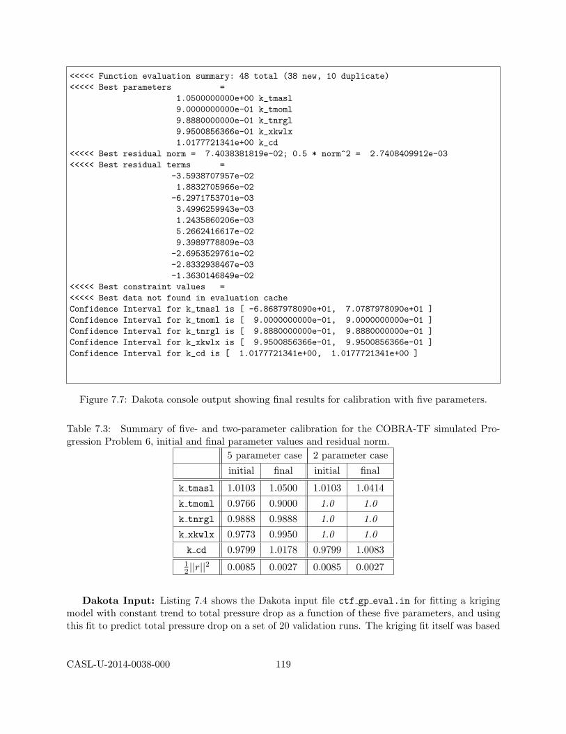
<<<<< Function evaluation summary: 48 total (38 new, 10 duplicate)<<<<< Best parameters =
1.0500000000e+00 k_tmasl9.0000000000e-01 k_tmoml9.8880000000e-01 k_tnrgl9.9500856366e-01 k_xkwlx1.0177721341e+00 k_cd
<<<<< Best residual norm = 7.4038381819e-02; 0.5 * norm^2 = 2.7408409912e-03<<<<< Best residual terms =
-3.5938707957e-021.8832705966e-02
-6.2971753701e-033.4996259943e-031.2435860206e-035.2662416617e-029.3989778809e-03
-2.6953529761e-02-2.8332938467e-03-1.3630146849e-02
<<<<< Best constraint values =<<<<< Best data not found in evaluation cacheConfidence Interval for k_tmasl is [ -6.8687978090e+01, 7.0787978090e+01 ]Confidence Interval for k_tmoml is [ 9.0000000000e-01, 9.0000000000e-01 ]Confidence Interval for k_tnrgl is [ 9.8880000000e-01, 9.8880000000e-01 ]Confidence Interval for k_xkwlx is [ 9.9500856366e-01, 9.9500856366e-01 ]Confidence Interval for k_cd is [ 1.0177721341e+00, 1.0177721341e+00 ]
Figure 7.7: Dakota console output showing final results for calibration with five parameters.
Table 7.3: Summary of five- and two-parameter calibration for the COBRA-TF simulated Pro-gression Problem 6, initial and final parameter values and residual norm.
5 parameter case 2 parameter case
initial final initial final
k tmasl 1.0103 1.0500 1.0103 1.0414
k tmoml 0.9766 0.9000 1.0 1.0
k tnrgl 0.9888 0.9888 1.0 1.0
k xkwlx 0.9773 0.9950 1.0 1.0
k cd 0.9799 1.0178 0.9799 1.008312 ||r||2 0.0085 0.0027 0.0085 0.0027
Dakota Input: Listing 7.4 shows the Dakota input file ctf gp eval.in for fitting a krigingmodel with constant trend to total pressure drop as a function of these five parameters, and usingthis fit to predict total pressure drop on a set of 20 validation runs. The kriging fit itself was based
CASL-U-2014-0038-000 119

on the results of using Dakota to run COBRA-TF on a Latin hypercube sample of size N = 50. Theoutput of these COBRA-TF runs was written to the file dakota pstudy.dat, which is subsequentlyread into this job via the import points option (line 35).
Results and Discussion: Figure 7.8 compares the emulator predictions with the COBRA-TF calculations of total pressure drop for the 20 validation runs. The left panel plots predictedvalue against calculated value, with the resulting points falling very close to the desired 45◦ line.The right panel plots the standardized residuals (calculated minus predicted total pressure dropdivided by standard error of predicted total pressure drop) against calculated value, indicatinga fairly constant scatter in the standardized residuals around the zero line across the spectrumof calculated values. This result is desirable in that it both indicates unbiased prediction andsupports the assumption of a homogeneous (constant) process variance σ2. Furthermore, we canapply a simple screening procedure for outliers to this standardized residual plot. First computethe interquartile range (IQR) of the standardized residuals, defined as the 75-th percentile minusthe 25-th percentile of the standardized residuals. Second compute lower and upper bounds asthe 25-th percentile minus 1.5× IQR and the 75-th percentile plus 1.5× IQR, respectively. Anystandardized residuals falling outside these bounds are flagged for further investigation as potentialoutliers. For this kriging fit, the lower and upper bounds calculated in this way were (-2.40, 3.38),while the range of the standardized residuals themselves was well within these bounds at (-1.33,2.38).
●●
●
●
●
●
●
●
●●
●
●
●
●●
●●
●
●
●
1.10 1.15 1.20 1.25
1.10
1.15
1.20
1.25
Calculated Total Pressure Drop
Pre
dict
ed T
otal
Pre
ssur
e D
rop
●
●
●
●
●
●
●
●
●
●
●
●
●
●●
●
●
●
●
●
1.10 1.15 1.20 1.25
−1
01
2
Calculated Total Pressure Drop
Sta
ndar
dize
d R
esid
ual T
otal
Pre
ssur
e D
rop
Figure 7.8: Predicted vs. calculated total pressure drop (left panel) and standardized residual vs.calculated total pressure drop (right panel) for 20 validation runs (red circles).
The leave-one-out cross-validation RMSPE of this kriging emulator, requested with the optionpress (line 34), evaluated to 3.2415584202e-04. When validation samples are available, as in thisexample, they can be used to compute a validation RMSPE. For Nv validation samples, calculate
RMSPE =
√√√√ 1Nv
Nv∑i=1
(Ci − Pi)2 ,
CASL-U-2014-0038-000 120

Listing 7.4: Dakota input file producing predictions for 20 validation runs from a GP emulator withestimated constant trend for the COBRA-TF simulated Progression Problem 6.# Build and evaluate a Gaussian process emulator of COBRA -TF output
2 # at a user specified set of points
4 strategy
single_method
6 method_pointer = ’EvalSurrogate ’
tabular_graphics_data
8 tabular_graphics_file = ’ctf_gp_evals.dat ’
10 # Method to perform evaluations of the emulator
12 method
id_method = ’EvalSurrogate ’
14 model_pointer = ’SurrogateModel ’
16 # Verbose will show the type form of the surrogate model
output verbose
18
sampling
20 sample_type lhs
samples = 20
22 seed = 150
24 # Surrogate model specification
model
26 id_model = ’SurrogateModel ’
surrogate global
28 # GP model
gaussian_process surfpack
30 trend
constant
32 # compute and print diagnostics after build
metrics ’rsquared ’ ’root_mean_squared ’
34 press
import_points = ’dakota_pstudy.dat ’ annotated
36
variables ,
38 uniform_uncertain = 5
upper_bounds 1.05 1.1 1.1 1.1 1.1
40 lower_bounds 0.95 0.9 0.9 0.9 0.9
descriptors ’k_tmasl ’ ’k_tmoml ’ ’k_tnrgl ’ ’k_xkwlx ’ ’k_cd ’
42
responses
44 response_functions = 1
descriptors = ’TotalPressure ’
46 no_gradients
no_hessians
CASL-U-2014-0038-000 121

where Pi and Ci denote the i-th predicted and calculated values, respectively. For our validationsample of Nv = 20, the RMSPE evaluates to 2.508674e-04. These RMSPE values are 0.15%and 0.11% of the observed range in the 20 calculated total pressure drops, indicating the krigingemulator possesses high accuracy for this application.
The assumption of Gaussian errors can be checked by examining normal probability plots ofthe standardized residuals from both leave-one-out cross validation and out-of-sample validation.Figure 7.9 shows normal probability plots for both of these cases. Theoretical quantiles from thestandard normal distribution are plotted on the x-axis, while the corresponding sample quantiles ofthe standardized residuals are plotted on the y-axis. Consistency with the Gaussian error assump-tion is indicated by the plotted points exhibiting strong linear association. The simple correlationcoefficients for the two cases are 0.992 and 0.965, respectively, suggesting that the Gaussian errorassumption is reasonable. The standardized residuals resulting from leave-one-out cross validationare correlated, making the normal probability plot somewhat harder to interpret as the theoreti-cal quantiles are calculated assuming independence. On the other hand, for the validation runs,the residuals were transformed to obtain uncorrelated standardized residuals for use in the normalprobability plot [6].
●
●
●
●
●
●
●
●
●
●
●
●
●
●
●
●
●
●
●
●●
●
●
●
●
●
●●
●●
●
●
●
●
●
●
●
●
●
●●
●
●
●
●●●
●
●
●
−2 −1 0 1 2
−2
−1
01
Leave−one−out Cross Validation
Theoretical Quantiles
Sam
ple
Qua
ntile
s
●
●
●
● ●
●●
●
●
●
●
●
●
●
●
●
●
●●
●
−2 −1 0 1 2
−1
01
2
Out−of−sample Validation
Theoretical Quantiles
Sam
ple
Qua
ntile
s
Figure 7.9: Normal probability plots based on standardized residuals from leave-one-out crossvalidation (left panel) and out-of-sample validation (right panel).
7.3.3 Bayesian Calibration
We illustrate here the use and verification of the Bayesian model calibration techniques, discussedin Section 6.2, for COBRA-TF. We focus on the parameters k tmasl, k tmoml, k tnrgl, k xkwlx,and k cd which, as detailed in the sensitivity analysis of Section 7.2, had non-negligible values forthe Morris elementary effect statistics. The synthetic data of Section 7.3, generated as detailed inSection 6.2.5, is consistent with the likelihoods employed in DRAM, DREAM, and GPMSA.
Analysis reveals that the total pressure drop can be accurately quantified by a linear relation
CASL-U-2014-0038-000 122
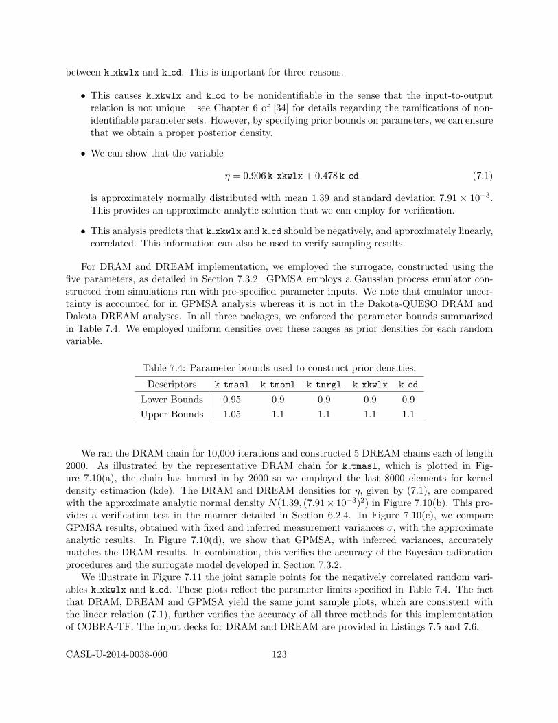
between k xkwlx and k cd. This is important for three reasons.
• This causes k xkwlx and k cd to be nonidentifiable in the sense that the input-to-outputrelation is not unique – see Chapter 6 of [34] for details regarding the ramifications of non-identifiable parameter sets. However, by specifying prior bounds on parameters, we can ensurethat we obtain a proper posterior density.
• We can show that the variable
η = 0.906 k xkwlx + 0.478 k cd (7.1)
is approximately normally distributed with mean 1.39 and standard deviation 7.91 × 10⁻³.This provides an approximate analytic solution that we can employ for verification.
• This analysis predicts that k xkwlx and k cd should be negatively, and approximately linearly,correlated. This information can also be used to verify sampling results.
For DRAM and DREAM implementation, we employed the surrogate, constructed using thefive parameters, as detailed in Section 7.3.2. GPMSA employs a Gaussian process emulator con-structed from simulations run with pre-specified parameter inputs. We note that emulator uncer-tainty is accounted for in GPMSA analysis whereas it is not in the Dakota-QUESO DRAM andDakota DREAM analyses. In all three packages, we enforced the parameter bounds summarizedin Table 7.4. We employed uniform densities over these ranges as prior densities for each randomvariable.
Table 7.4: Parameter bounds used to construct prior densities.
Descriptors k tmasl k tmoml k tnrgl k xkwlx k cd
Lower Bounds 0.95 0.9 0.9 0.9 0.9Upper Bounds 1.05 1.1 1.1 1.1 1.1
We ran the DRAM chain for 10,000 iterations and constructed 5 DREAM chains each of length2000. As illustrated by the representative DRAM chain for k tmasl, which is plotted in Fig-ure 7.10(a), the chain has burned in by 2000 so we employed the last 8000 elements for kerneldensity estimation (kde). The DRAM and DREAM densities for η, given by (7.1), are comparedwith the approximate analytic normal density N(1.39, (7.91× 10⁻³)2) in Figure 7.10(b). This pro-vides a verification test in the manner detailed in Section 6.2.4. In Figure 7.10(c), we compareGPMSA results, obtained with fixed and inferred measurement variances σ, with the approximateanalytic results. In Figure 7.10(d), we show that GPMSA, with inferred variances, accuratelymatches the DRAM results. In combination, this verifies the accuracy of the Bayesian calibrationprocedures and the surrogate model developed in Section 7.3.2.
We illustrate in Figure 7.11 the joint sample points for the negatively correlated random vari-ables k xkwlx and k cd. These plots reflect the parameter limits specified in Table 7.4. The factthat DRAM, DREAM and GPMSA yield the same joint sample plots, which are consistent withthe linear relation (7.1), further verifies the accuracy of all three methods for this implementationof COBRA-TF. The input decks for DRAM and DREAM are provided in Listings 7.5 and 7.6.
CASL-U-2014-0038-000 123

0 2000 4000 6000 8000 100000.95
0.96
0.97
0.98
0.99
1
1.01
1.02
1.03
1.04
1.05
Para
mete
r V
alu
e
Chain Index1.35 1.36 1.37 1.38 1.39 1.4 1.41 1.42 1.43 1.440
10
20
30
40
50
60
Parameter Value
DRAM
DREAM
Gaussian
(a) (b)
1.34 1.36 1.38 1.4 1.42 1.44 1.460
10
20
30
40
50
60
Parameter Value
Fixed Variance
Calibrated Variance
Gaussian
1.34 1.36 1.38 1.4 1.42 1.44 1.460
10
20
30
40
50
60
Parameter Value
DRAM
GPMSA
Gaussian
(c) (d)
Figure 7.10: (a) Representative DRAM chain for k tmasl showing burn-in by 2000. (b) Verificationof the densities for η provided by DRAM and DREAM through comparison with the analytic Gaus-sian solution. (c) and (d) Verification of GPMSA for fixed and inferred measurement variance σ.
It was noted in Section 6.2.3 that once Bayesian chains have been constructed, values from thechain can be used as inputs to surrogate models to compute calibrated predictions for additionalquantities of interest. This is illustrated in Figure 7.12, where we compare credible intervals for thetotal pressure drop computed using GPMSA with the surrogate model evaluated using inputs fromthe DRAM chain. The nominal total pressure drop value of 1.176 bar, computed using COBRA-TFwith nominal parameter values, lies within one standard deviation of the mean. Furthermore, theprediction is essentially Gaussian due to the linearity of the response in this operating regime. TheDakota input deck is provided in Listing 7.7 where one can note that it inputs DRAM values fromthe file ctf gp evals dram.dat.
CASL-U-2014-0038-000 124
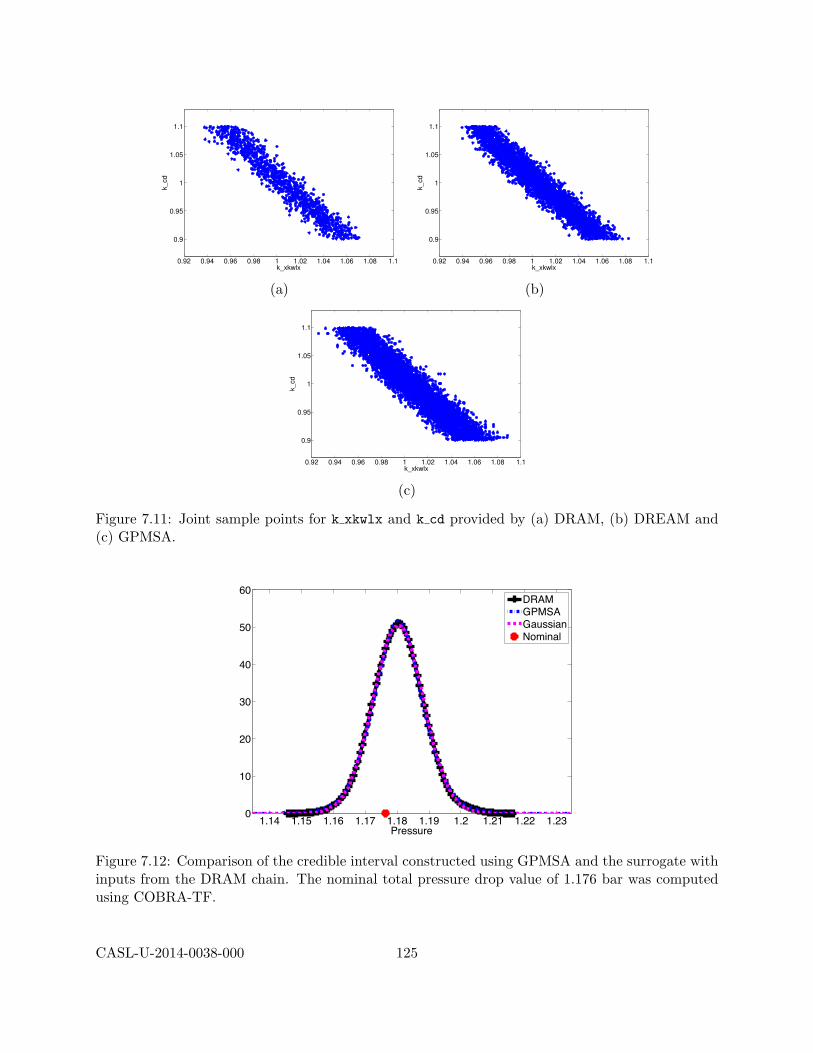
0.92 0.94 0.96 0.98 1 1.02 1.04 1.06 1.08 1.1
0.9
0.95
1
1.05
1.1
k_cd
k_xkwlx0.92 0.94 0.96 0.98 1 1.02 1.04 1.06 1.08 1.1
0.9
0.95
1
1.05
1.1
k_cd
k_xkwlx
(a) (b)
0.92 0.94 0.96 0.98 1 1.02 1.04 1.06 1.08 1.1
0.9
0.95
1
1.05
1.1
k_cd
k_xkwlx
(c)
Figure 7.11: Joint sample points for k xkwlx and k cd provided by (a) DRAM, (b) DREAM and(c) GPMSA.
1.14 1.15 1.16 1.17 1.18 1.19 1.2 1.21 1.22 1.230
10
20
30
40
50
60
Pressure
DRAMGPMSAGaussianNominal
Figure 7.12: Comparison of the credible interval constructed using GPMSA and the surrogate withinputs from the DRAM chain. The nominal total pressure drop value of 1.176 bar was computedusing COBRA-TF.
CASL-U-2014-0038-000 125

Listing 7.5: Input for Dakota-QUESO DRAM as applied to the COBRA-TF surrogate for Progres-sion Problem 6.
1 strategy
single_method
3
method
5 bayes_calibration queso
emulator
7 gaussian_process surfpack
import_points = ’dakota_5pstudy.dat ’ annotated
9 mcmc_type dram
rejection delayed
11 metropolis adaptive
samples = 10000
13 seed = 52983
15 variables
active design
17 continuous_design = 5
#initial_point 1.05 1.0 1.0 1.04
19 upper_bounds 1.05 1.1 1.1 1.1 1.1
lower_bounds 0.95 0.9 0.9 0.9 0.9
21 descriptors ’k_tmasl ’ ’k_tmoml ’ ’k_tnrgl ’ ’k_xkwlx ’ ’k_cd ’
23 interface
direct
25 analysis_driver = ’text_book ’
27 responses
calibration_terms = 1
29 calibration_data_file = ’ctf_dat.txt ’
freeform
31 num_experiments = 1
num_replicates = 10
33 num_std_deviations = 1
descriptors
35 ’TotalPressure ’
no_gradients
37 no_hessians
CASL-U-2014-0038-000 126
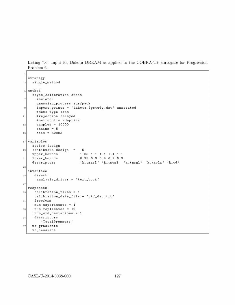
Listing 7.6: Input for Dakota DREAM as applied to the COBRA-TF surrogate for ProgressionProblem 6.
1
strategy
3 single_method
5 method
bayes_calibration dream
7 emulator
gaussian_process surfpack
9 import_points = ’dakota_5pstudy.dat ’ annotated
#mcmc_type dram
11 #rejection delayed
#metropolis adaptive
13 samples = 10000
chains = 5
15 seed = 52983
17 variables
active design
19 continuous_design = 5
upper_bounds 1.05 1.1 1.1 1.1 1.1
21 lower_bounds 0.95 0.9 0.9 0.9 0.9
descriptors ’k_tmasl ’ ’k_tmoml ’ ’k_tnrgl ’ ’k_xkwlx ’ ’k_cd ’
23
interface
25 direct
analysis_driver = ’text_book ’
27
responses
29 calibration_terms = 1
calibration_data_file = ’ctf_dat.txt ’
31 freeform
num_experiments = 1
33 num_replicates = 10
num_std_deviations = 1
35 descriptors
’TotalPressure ’
37 no_gradients
no_hessians
CASL-U-2014-0038-000 127

Listing 7.7: Dakota input used to construct credible interval for total pressure drop using DRAMevaluations.# Build and evaluate a Gaussian process emulator of COBRA -TF output
2 # at a user specified set of points
4 strategy
single_method
6 #environment
method_pointer = ’EvalSurrogate ’
8 tabular_graphics_data
tabular_graphics_file = ’ctf_gp_evals_dram.dat ’
10
# Method to perform evaluations of the emulator
12
method
14 id_method = ’EvalSurrogate ’
model_pointer = ’SurrogateModel ’
16
# Verbose will show the type form of the surrogate model
18 output verbose
20 list_parameter_study
import_points = ’dram_result.txt ’ freeform
22
# Surrogate model specification
24 model
id_model = ’SurrogateModel ’
26 surrogate global
# GP model
28 gaussian_process surfpack
trend
30 constant
# compute and print diagnostics after build
32 metrics ’rsquared ’ ’root_mean_squared ’
press
34 import_points = ’dakota_5pstudy.dat ’ annotated
36 variables ,
uniform_uncertain = 5
38 upper_bounds 1.05 1.1 1.1 1.1 1.1
lower_bounds 0.95 0.9 0.9 0.9 0.9
40 descriptors ’k_tmasl ’ ’k_tmoml ’ ’k_tnrgl ’ ’k_xkwlx ’ ’k_cd ’
42 responses
response_functions = 1
44 descriptors = ’TotalPressure ’
no_gradients
46 no_hessians
CASL-U-2014-0038-000 128

Appendix A
General Linear Model VerificationTest Suite
This appendix provides additional technical details for the linear model introduced in Section 2.2.Here we describe in detail a particular class of problems for which results of the QUESO DRAM orDakota DREAM sampling algorithm can be verified against analytical solutions. Specifically, wepresent standard results for Bayesian analysis of the linear regression model ([11], pp. 233-265). Inlinear regression, a N -vector of outputs y is related linearly to functions of inputs x,
y = Gβ + ε ,
where the i-th row of G contains the evaluation of these regression functions at input xi corre-sponding to the i-th datum yi, β denotes the regression coefficients, and ε denotes the vector ofobservational errors. In the following, observational errors will be assumed mean-zero Gaussian,having variance (1/λ) and possibly correlated with parametric dependencies goverened by a pa-rameter φ.
Marginal posterior distributions for β, λ, and φ are derived analytically for three increasinglychallenging verification scenarios: (i) β unknown, (λ, φ) fixed; (ii) (β, λ) unknown, φ fixed; and(iii) (β, λ, φ) unknown. In the third scenario, the marginal posterior distributions of β, λ, and φdo not belong to a standard class of probability distributions (such as Gaussian or Gamma, forexample), thus requiring the use of numerical methods such as quadrature to accurately estimatetheir normalizing constants.
For each verification scenario, QUESO samples from the applicable marginal posterior distri-butions for β, λ, and φ will be compared with the corresponding analytical results. Convergenceof posterior means and other summary statistics to corresponding parameter values assumed fordata generation will also be monitored for a subset of the observational error correlation structuresinvestigated.
Section A.1 describes how data are simulated and presents the three verification scenarios ofinterest with corresponding analytical results for the desired posterior distributions in each scenario.Section A.2 defines the verification tests currently implemented.
CASL-U-2014-0038-000 129

A.1 Verification Scenarios
Let εt denote a mean-zero Gaussian stochastic process having covariance function c(t1, t2|φ) =(1/λ) r(t1, t2|φ), where λ > 0 and r(·, ·|φ) is a correlation function for φ ∈ Φ. We assume thefollowing quantities are specified:
1. Nominal parameter settings (β0, λ0, φ0) with β0 ∈ <Nβ , λ0 > 0, and φ0 ∈ int(Φ)
2. Indices {t1, t2, . . . , tN}.We denote the multivariate Gaussian distribution having location vector µ and covariance matrixΣ by N (µ,Σ). For specified N , generate a N -vector of errors
(εt1 , . . . , εtN ) ∼ N (0N , (1/λ0)R(φ0)) ,
where 0N is the N -vector of zeroes and the (i, j) element of R(φ0) is given by r(ti, tj |φ0). To com-plete the data generation process, we sample M -dimensional covariates {X1, . . . XN} independentlyfrom the distribution N (0M , C), where C is a fixed covariance matrix. The i-th datum is calculatedas yti = gT (xi)β0 + εti , where g(·) is a Nβ-dimensional regression function. In vector-matrix form,
y = Gβ0 + ε ,
where
y = (yt1 , yt2 , . . . , ytN )T ,
G = [ g(x1) g(x2) · · · g(xN ) ]T , and
ε = (εt1 , εt2 , . . . , εtN )T .
To generate N additional responses, we sample:
1. {XN+1, . . . , XN+N} independently from the distribution N (0M , C)
2. (εtN+1 , . . . , εtN+N)T ∼ N
(0N , (1/λ0)
(R(φ0)− R(φ0)R−1(φ0)RT (φ0)
)),
where the (i, j) element of R(φ0) is given by r(tN+i, tN+j |φ0), and the (i, j) element of R(φ0) is givenby r(tN+i, tj |φ0). Then ytN+i = gT (xN+i)β0 + εtN+i and the matrix-vector form of the augmenteddata set follows. Note that this process of conditionally sampling errors preserves the correct jointdisribution of the augmented data vector.
In the following calculations, we assume the regression matrix G is fixed, so this will not beexplicitly denoted in the notation. Although (β, λ, φ) are fixed at (β0, λ0, φ0) to generate data asabove, our statistical analyses will assume some or all of (β0, λ0, φ0) are unknown. The samplingdistribution f(Y |β, λ, φ) of a random data set Y of size N is N (Gβ, (1/λ)R(φ)).
(Case 1.) The first verification scenario assumes that λ and φ are fixed at λ0 and φ0, respec-tively. The Bayesian analysis places a prior distribution on β, which is given by the following:
1. π(β) =∫<Nβ
π(β|µ)π(µ) dµ,
2. π(β|µ) is N (µ, λ−10 Σ−1), and
CASL-U-2014-0038-000 130

3. π(µ) is N (µ0, λ−10 Σ−1
0 ).
These assumptions imply that the marginal prior π(β) is N (µ0, λ−10
(Σ−1
0 + Σ−1))
.The posterior distribution of µ is N (µ1(φ0), λ−1
0 Σ1(φ0)), where
Σ−11 (φ0) = Σ0 +
(Σ−1 +
(GTR−1(φ0)G
)−1)−1
and
µ1(φ0) = Σ1(φ0)[(
Σ−1 +(GTR−1(φ0)G
)−1)−1
β(φ0) + Σ0µ0
]for β(φ0) =
(GTR−1(φ0)G
)−1GTR−1(φ0) y.
The posterior distribution of β is N (µ2(φ0), λ−10 Σ2(φ0)
), where
Σ−12 (φ0) =
(Σ−1
0 + Σ−1)−1 +GTR−1(φ0)G and
µ2(φ0) = Σ2(φ0)[(GTR−1(φ0)G
)β(φ0) +
(Σ−1
0 + Σ−1)−1
µ0
].
A noninformative prior for β, π(β) ∝ 1, results in an improper posterior distribution of µ. Notethat assuming a noninformative prior for µ, π(µ) ∝ 1, implies π(β) ∝ 1. The posterior distributionof β is as above, with
µ2(φ0) = β(φ0) and Σ2(φ0) =(GTR−1(φ0)G
)−1. (A.1)
The predictive distribution of Q future responses Y = (Yt1 , Yt2 , . . . , YtQ)T associated with regres-sion matrix G = [ g(x1) g(x2) · · · g(xQ)]T and the Q-variate error vector εQ = (εt1 , εt2 , . . . , εtQ)T
is N(µ(φ0), λ−1
0 Σ(φ0))
, where
µ(φ0) = Gµ2(φ0) + R(φ0)R−1(φ0) (y −Gµ2(φ0)) and
Σ(φ0) = R(φ0)− R(φ0)R−1(φ0)RT (φ0) + H(φ0)Σ2(φ0)H(φ0)T
for H(φ0) = G− R(φ0)R−1(φ0)G. Here, the (i, j) element of R(φ0) is given by r(ti, tj |φ0), and the(i, j) element of R(φ0) is given by r(ti, tj |φ0).
(Case 2.) The second verification scenario assumes that φ is fixed at φ0. The Bayesian analysisplaces a prior distribution on (β, λ), which is given by the following:
1. π(β|λ) =∫<Nβ
π(β|µ, λ)π(µ|λ) dµ,
2. π(β|µ, λ) is N (µ, λ−1Σ−1),
3. π(µ|λ) is N (µ0, λ−1Σ−1
0 ), and
4. π(λ) is Gamma(a, b).
These assumptions imply that the marginal prior π(β|λ) is N (µ0, λ−1(Σ−1
0 + Σ−1))
.
CASL-U-2014-0038-000 131

The posterior distribution of λ is Gamma(a1, b1(φ0)), where
a1 = (2a+N)/2
b1(φ0) =(
2b+(y −Gβ(φ0)
)TR−1(φ0)
(y −Gβ(φ0)
)+(β(φ0)− µ0
)TΣ−1
3 (φ0)(β(φ0)− µ0
))/2
for Σ3(φ0) = Σ−10 + Σ−1 +
(GTR−1(φ0)G
)−1.A noninformative prior for β, π(β) ∝ 1, results in the posterior distribution of λ given above,
with
a1 = (2a+N −Nβ)/2 and b1(φ0) =(
2b+(y −Gβ(φ0)
)TR−1(φ0)
(y −Gβ(φ0)
))/2 . (A.2)
A noninformative prior for λ, π(λ) ∝ (1/λ), results from taking a = b = 0. Note that π(β, λ) ∝(1/λ) is the Jeffreys noninformative prior.
We denote the d-variate t distribution having ν degrees of freedom, location vector µ, and scalematrix Σ by Td(ν, µ,Σ). The mean of this distribution is µ if ν > 1 and the covariance matrix ofthis distribution is νΣ/(ν − 2) if ν > 2. The posterior distributions of µ and β are given by
π(µ|y) is TNβ (2a1, µ1(φ0), b1(φ0)Σ1(φ0)/a1)
π(β|y) is TNβ (2a1, µ2(φ0), b1(φ0)Σ2(φ0)/a1) .
For the noninformative prior π(β) ∝ 1, as before the posterior distribution of µ is improper. Thequantities µ2(φ0), Σ2(φ0) from (A.1) and a1, b1(φ0) from (A.2) are utilized in the above expressionfor the posterior distribution of β, where again a = b = 0 for π(λ) ∝ (1/λ).
The predictive distribution of Y is given by
π(Y |y) is TQ(
2a1, µ(φ0), b1(φ0)Σ(φ0)/a1
).
(Case 3.) The third verification scenario allows φ to be random. The Bayesian analysis placesa prior distribution on (β, λ, φ), which is given by π(β, λ, φ) = π(β, λ)π(φ) where π(β, λ) is specifiedas in the previous scenario. The form of π(φ) used in verification testing will be provided in thefollowing section. Our goal in this scenario is to numerically approximate the marginal posteriordistributions of λ, µ, and β:
π(λ|y) =∫
Φπ(λ|y, φ)π(φ|y) dφ
π(µ|y) =∫
Φπ(µ|y, φ)π(φ|y) dφ
π(β|y) =∫
Φπ(β|y, φ)π(φ|y) dφ .
The distributions π(λ|y, φ), π(µ|y, φ), and π(β|y, φ) are given analytically in the previous scenario.That leaves π(φ|y), which is given as follows:
π(φ|y) ∝ π(φ)
b1(φ)a1 det (R(φ))1/2 det (GTR−1(φ)G)1/2 det (Σ3(φ))1/2.
CASL-U-2014-0038-000 132

Quadrature is used to compute the normalizing constant
c(y) =∫
Φ
π(φ) dφ
b1(φ)a1 det (R(φ))1/2 det (GTR−1(φ)G)1/2 det (Σ3(φ))1/2
so that
π(φ|y) =c−1(y)π(φ)
b1(φ)a1 det (R(φ))1/2 det (GTR−1(φ)G)1/2 det (Σ3(φ))1/2.
For the noninformative prior π(β) ∝ 1,
π(φ|y) =c−1(y)π(φ)
b1(φ)a1 det (R(φ))1/2 det (GTR−1(φ)G)1/2
forc(y) =
∫Φ
π(φ) dφ
b1(φ)a1 det (R(φ))1/2 det (GTR−1(φ)G)1/2,
where a1, b1(φ) are taken from (A.2) and a = b = 0 for π(λ) ∝ (1/λ).The predictive distribution of Y can also be numerically approximated:
π(Y |y) =∫
Φπ(Y |y, φ)π(φ|y) dφ .
A.2 Verification Tests
A simple linear regression model, g(x) = (1, x1, x2, . . . , xM )T , is specified for all verification ex-amples. The dimension of β is therefore Nβ = M + 1. A wide range of covariate dimensions areconsidered, M ∈ {2, 10, 50, 100, 500, 1000}.
The verification examples proceed by considering successively more complex specifications ofthe correlation function r(t1, t2|φ):
1. r(ti, tj) = δti,tj
2. r(ti, tj |φ) = δti,tj + φ(1− δti,tj ), φ ∈ [0, 1)
3. r(ti, tj |φ) = φ|i−j|, −1 < φ < 1
4. r(ti, tj |φ) = exp[−(xi − xj)TDφ(xi − xj)
], where Dφ = diag(φ1, . . . , φNβ ) and φi ≥ 0 for
i = 1, . . . , Nβ.
The first case describes the standard regression setting in which errors are uncorrelated. The secondcase describes equi-correlated errors, for which all pairwise correlations are equal. The third casedescribes an AR(1) correlation structure for errors associated with observations indexed by time.The pairwise correlation between errors decays as a function of separation in time. The final casespecifies a Gaussian correlation for errors associated with observations indexed by covariates. Thepairwise correlation between errors decays as a function of weighted distance between the covariatevectors associated with the corresponding observations.
The first three correlation functions admit explicit expressions for the inverse R−1(φ) and de-terminant det (R(φ)),
CASL-U-2014-0038-000 133

1. IN and 1
2. 11−φ
[IN − φ
1+(N−1)φJN]
and (1− φ)N−1(1 + (N − 1)φ)
3. 11−φ2
1 −φ 0 0 · · · 0 0−φ 1 + φ2 −φ 0 · · · 0 00 −φ 1 + φ2 −φ · · · 0 0...
......
......
......
0 0 0 0 · · · 1 + φ2 −φ0 0 0 0 · · · −φ 1
and (1− φ2)N−1 ,
where IN is the N ×N identity matrix and JN is the N ×N matrix of ones.For data sample sizes, we consider {1, 2, 3, 10, 100, 1000, 104, 105, 106} for the first three correla-
tion functions, and {1, 2, 3, 10, 100, 1000} for the fourth correlation function (sample size limited byinverse and determinant calculations). Small sample sizes {1, 2, 3} will allow MCMC sampling fromheavy-tailed posterior distributions to be compared with known analytical forms (specifically, themultivariate t distributions of the second and third analyses). Large sample sizes allow verificationof regression parameter and error variance point estimate convergence (β → β0 and b1/a1 → λ−1
0 )for the first correlation function. Each case will be structured so that the number of random pa-rameters does not exceed the sample size. For example, if N = 1, only the first scenario is analyzedwith a single random regression parameter β0.
Two prior specifications will be considered: (a) π(µ, β, λ) ∝ (1/λ) (noninformative) and (b)Σ0 = q INβ for fixed 0 < q � 1, and Σ = diag({ri, i = 1, . . . , Nβ}) for fixed ri > 0 (proper).Both cases take a = b = 0. For the first correlation function, case (b) allows verification of theconvergence of the posterior distribution of µ to the Gaussian distribution having mean vector andcovariance matrix
µ1 = Dββ0 +Dµµ0 and λ−10 Σ1 = diag({λ−1
0 /(q + ri), i = 1, . . . , Nβ})
where Dβ = diag({ri/(q+ ri), i = 1, . . . , Nβ}) and Dµ = diag({q/(q+ ri), i = 1, . . . , Nβ}). For eachof these cases, we take π(φ) ∝ 1 for the second and third correlation function options. For thefourth option, assume the inputs x satisfy ` ≤ x ≤ u and let ρi = ρi(φ) = exp
[−φ(ui − `i)2/4]
forφ ≥ 0. The parameter ρi ∈ (0, 1] represents a correlation length, and we take ρi ∼ Beta(aρ, bρ) with(aρ, bρ) = (1, 0.1) independently for i = 1, . . . ,M as the prior distribution for ρ = (ρ1, . . . , ρM ). Wethen have
π(φ) ∝M∏i=1
[ρi(φi)]aρ [1− ρi(φi)]bρ−1 χ[0,∞)(φi)
where χ[0,∞)(φ) is the characteristic function taking value 1 for φ ≥ 0 and 0 for φ < 0.Bayesian calibration results for these examples are detailed in Section 6.2.6.
CASL-U-2014-0038-000 134

Appendix B
Procedure for Running COBRA-TFStudies
This section provides a brief description of how to perform the COBRA-TF studies described inChapter 7 with the model detailed in Section 2.3 on one of the CASL compute machines using theVERA software environment. This assumes that the steps necessary to log on to one of the variousCASL machines, e.g. u233, u235, etc., have been successfully completed.
At present there are two choices for running a VERA VUQ study. One choice is to use the“mainline” codes and utilities that are formally part of the VERA-CS software. This code is testednightly and adheres to the software quality standards defined by VERA-CS. The alternative is touse an extended capability representing the most current development activities but which is notincluded in VERA nightly testing. This code and utilities reside in a collection of repositories forkedfrom the mainline. Regardless of which choice is made, the following project directory structure isrequired:
VERA|-- Trilinos| || -- packages| || -- TriKota| || -- Dakota|-- COBRA-TF|-- VERAInExt|-- LIMEExt|-- PSSDriversExt|-- VUQDemos
Table B.1 shows the locations from which to clone each repository for either choice.
CASL-U-2014-0038-000 135
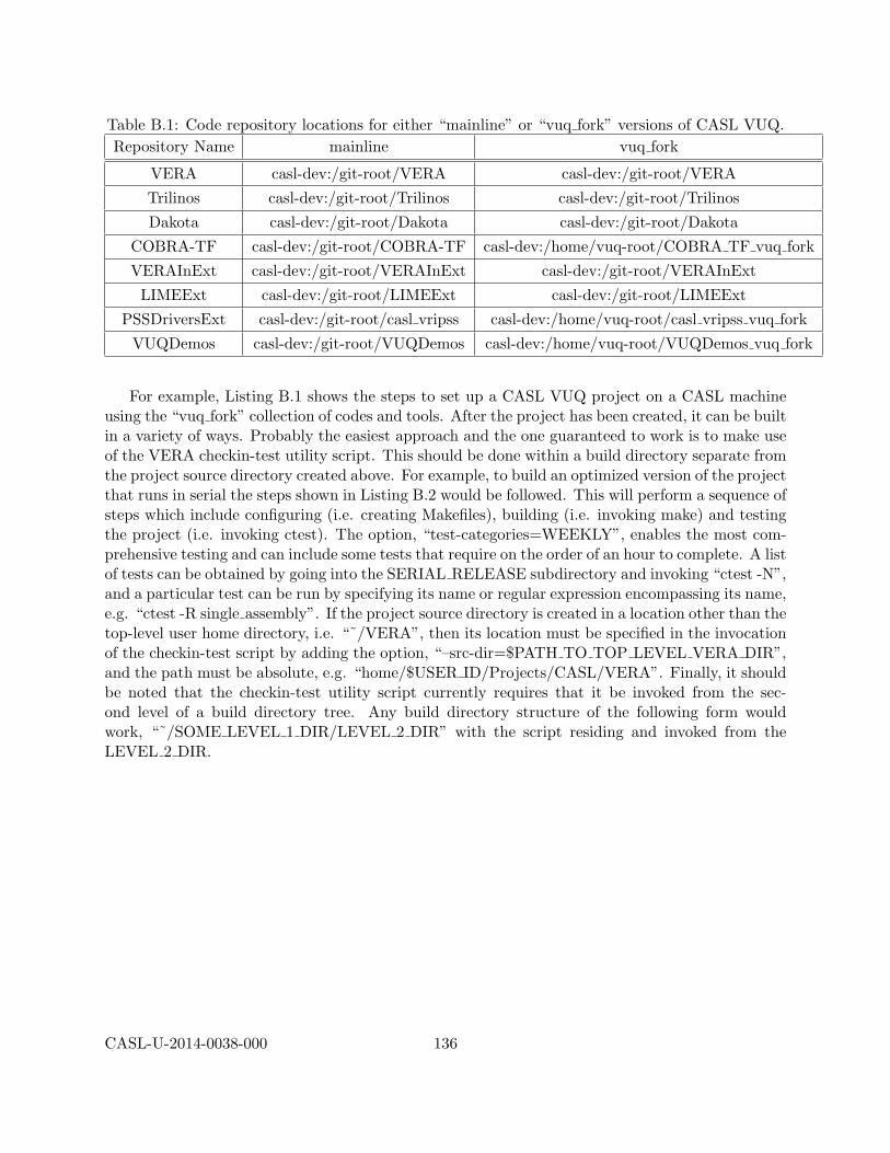
Table B.1: Code repository locations for either “mainline” or “vuq fork” versions of CASL VUQ.Repository Name mainline vuq fork
VERA casl-dev:/git-root/VERA casl-dev:/git-root/VERA
Trilinos casl-dev:/git-root/Trilinos casl-dev:/git-root/Trilinos
Dakota casl-dev:/git-root/Dakota casl-dev:/git-root/Dakota
COBRA-TF casl-dev:/git-root/COBRA-TF casl-dev:/home/vuq-root/COBRA TF vuq fork
VERAInExt casl-dev:/git-root/VERAInExt casl-dev:/git-root/VERAInExt
LIMEExt casl-dev:/git-root/LIMEExt casl-dev:/git-root/LIMEExt
PSSDriversExt casl-dev:/git-root/casl vripss casl-dev:/home/vuq-root/casl vripss vuq fork
VUQDemos casl-dev:/git-root/VUQDemos casl-dev:/home/vuq-root/VUQDemos vuq fork
For example, Listing B.1 shows the steps to set up a CASL VUQ project on a CASL machineusing the “vuq fork” collection of codes and tools. After the project has been created, it can be builtin a variety of ways. Probably the easiest approach and the one guaranteed to work is to make useof the VERA checkin-test utility script. This should be done within a build directory separate fromthe project source directory created above. For example, to build an optimized version of the projectthat runs in serial the steps shown in Listing B.2 would be followed. This will perform a sequence ofsteps which include configuring (i.e. creating Makefiles), building (i.e. invoking make) and testingthe project (i.e. invoking ctest). The option, “test-categories=WEEKLY”, enables the most com-prehensive testing and can include some tests that require on the order of an hour to complete. A listof tests can be obtained by going into the SERIAL RELEASE subdirectory and invoking “ctest -N”,and a particular test can be run by specifying its name or regular expression encompassing its name,e.g. “ctest -R single assembly”. If the project source directory is created in a location other than thetop-level user home directory, i.e. “˜/VERA”, then its location must be specified in the invocationof the checkin-test script by adding the option, “–src-dir=$PATH TO TOP LEVEL VERA DIR”,and the path must be absolute, e.g. “home/$USER ID/Projects/CASL/VERA”. Finally, it shouldbe noted that the checkin-test utility script currently requires that it be invoked from the sec-ond level of a build directory tree. Any build directory structure of the following form wouldwork, “˜/SOME LEVEL 1 DIR/LEVEL 2 DIR” with the script residing and invoked from theLEVEL 2 DIR.
CASL-U-2014-0038-000 136

Listing B.1: Steps to setup a vuq fork CASL VUQ project on one of the CASL machines
2 # Checkout top -level VERA source directory
git clone casl -dev:/git -root/VERA
4
# Checkout Trilinos under VERA
6 cd VERA
git clone casl -dev:/git -root/Trilinos
8
# Checkout Dakota in proper subdirectory under Trilinos
10 cd Trilinos/packages/TriKota
git clone casl -dev:/git -root/Dakota
12
# Checkout Cobra -TF Thermal Hydraulics code under VERA
14 cd ../../../
git clone casl -dev:/home/vuq -root/COBRA_TF_vuq_fork COBRA -TF
16
# Checkout VERA Common Input toolset under VERA
18 git clone casl -dev:/git -root/VERAInExt
20 # Checkout LIME multi -physics coupling driver under VERA
git clone casl -dev:/git -root/LIMEExt
22
# Checkout VERA interfaces to CASL application codes under VERA
24 git clone casl -dev:/home/vuq -root/casl_vripss_vuq_fork PSSDriversExt
26 # Checkout CASL VUQ toolset under VERA
git clone casl -dev:/home/vuq -root/VUQDemos_vuq_fork VUQDemos
Listing B.2: Steps to build a vuq fork CASL VUQ project on one of the CASL machines1
# Create a build directory
3 mkdir -p CASL_BUILDS/VUQ_BUILD
cd CASL_BUILDS/VUQ_BUILD
5
# Create a link to the checkin -test utility script in the source project directory
7 ln -s ~/VERA/cmake/ctest/drivers/fissile4/checkin -test -vera.sh
9 # Invoke the script to build an optimized serial version of the project
./checkin -test -vera.sh --extra -repos -type=Nightly --test -categories=WEEKLY \
11 --default -builds=SERIAL_RELEASE --enable -packages=VUQDemos --local -do-all
CASL-U-2014-0038-000 137
Bibliography
[1] B. M. Adams, L. E. Bauman, W. J. Bohnhoff, K. R. Dalbey, J. P. Eddy, M. S. Ebeida, M. S.Eldred, P. D. Hough, K. T. Hu, J. D. Jakeman, L. P. Swiler, and D. M. Vigil. Dakota, amultilevel parallel object-oriented framework for design optimization, parameter estimation,uncertainty quantification, and sensitivity analysis: Version 5.4 user’s manual. Technical Re-port SAND2010-2183, Sandia National Laboratories, Albuquerque, NM, Updated Nov. 2013.Available online from http://dakota.sandia.gov/documentation.html.
[2] B. M. Adams, L. E. Bauman, W. J. Bohnhoff, K. R. Dalbey, J. P. Eddy, M. S. Ebeida, M. S.Eldred, P. D. Hough, K. T. Hu, J. D. Jakeman, L. P. Swiler, and D. M. Vigil. Dakota, amultilevel parallel object-oriented framework for design optimization, parameter estimation,uncertainty quantification, and sensitivity analysis: Version 5.4 reference manual. Techni-cal Report SAND2010-2184, Sandia National Laboratories, Albuquerque, NM, Updated Nov.2013. Available online from http://dakota.sandia.gov/documentation.html.
[3] B. M. Adams, L. E. Bauman, W. J. Bohnhoff, K. R. Dalbey, J. P. Eddy, M. S. Ebeida, M. S.Eldred, P. D. Hough, K. T. Hu, J. D. Jakeman, L. P. Swiler, and D. M. Vigil. Dakota, amultilevel parallel object-oriented framework for design optimization, parameter estimation,uncertainty quantification, and sensitivity analysis: Version 5.4 theory manual. Technical Re-port SAND2011-9106, Sandia National Laboratories, Albuquerque, NM, Updated Nov. 2013.Available online from http://dakota.sandia.gov/documentation.html.
[4] J. S. Arora. Introduction to Optimum Design. McGraw-Hill, New York, 1989.
[5] M. N. Avramova. CTF: A thermal hydraulic sub-channel code for LWR transient analyses,users manual. Technical report, Pennsylvania State University, February 2009.
[6] L. S. Bastos and A. O’Hagan. Diagnostics for Gaussian process emulators. Technometrics,51:425–438, 2009.
[7] G. E. P. Box and D. W. Behnken. Some new three level designs for the study of quantitativevariables. Technometrics, 2:455–475, 1958.
[8] G. E. P. Box and K. B. Wilson. On the experimental attainment of optimum conditions (withdiscussion). Journal of the Royal Statistical Society Series B, 13:1–45, 1951.
[9] N. Cressie. Statistics of Spatial Data. John Wiley and Sons, New York, 1991.
[10] K. R. Dalbey, A. A. Giunta, M. D. Richards, E. C. Cyr, L. P. Swiler, S. L. Brown, M. S. Eldred,and B. M. Adams. Surfpack user’s manual: Version 1.1. Technical report, Sandia National
CASL-U-2014-0038-000 138

Laboratories, Albuquerque, NM, 2006. Available online from http://dakota.sandia.gov/packages/Surfpack.
[11] A. Gelman, J. B. Carlin, H. S. Stern, and D. B. Rubin. Bayesian Data Analysis. Chapman &Hall/CRC, Boca Raton, 1997.
[12] R. Ghanem and J. R. Red-Horse. Propagation of probabilistic uncertainty in complex physicalsystems using a stochastic finite element technique. Physica D, 133:137–144, 1999.
[13] R. G. Ghanem and P. D. Spanos. Stochastic Finite Elements: A Spectral Approach. Springer-Verlag, New York, 1991.
[14] P. E. Gill, W. Murray, and M. H. Wright. Practical Optimization. Academic Press, San Diego,CA, 1981.
[15] Heikki Haario, Marko Laine, Antonietta Mira, and Eero Saksman. DRAM: Efficient adaptiveMCMC. Statistics and Computing, 16:339–354, 2006.
[16] R. T. Haftka and Z. Gurdal. Elements of Structural Optimization. Kluwer, Boston, 1992.
[17] W. E. Hart. The Coliny project. Web site, 2007.
[18] A. S. Hedayat, N. J. A. Sloane, and J. Stufken. Orthogonal Arrays: Theory and Applications.Springer, New York, 1999.
[19] D. Higdon, J. Gattiker, B. Williams, and M. Rightley. Computer model calibration usinghigh-dimensional output. Journal of the American Statistical Association, 103(482):570–583,2008.
[20] E. T. Jaynes and G. Larry Bretthorst. Probability theory : the logic of science. CambridgeUniversity Press, Cambridge, UK; New York, NY, 2003.
[21] C. T. Kelley. Implicit Filtering. SIAM, 2011.
[22] M. C. Kennedy and A. O’Hagan. Bayesian calibration of computer models. Journal of theRoyal Statistical Society, 63:425–464, 2001.
[23] J. L. Loeppky, J. Sacks, and W. J. Welch. Choosing the sample size of a computer experiment:A practial guide. Technometrics, 51:366–376, 2009.
[24] G. Matheron. The theory of regionalized variables and its applications. Les Cahiers du Centrede morphologie mathematique de Fontainebleau. Ecole national superieure des mines, 1971.
[25] M. D. Morris. Factorial sampling plans for preliminary computational experiments. Techno-metrics, 33(2):161–174, 1991.
[26] V. A. Mousseau et al. VUQ strategy. Technical Report CASL-U-2014-XXXX-YYY, Oak RidgeNational Laboratory, March 2014. In preparation.
[27] R. H. Myers and D. C. Montgomery. Response Surface Methodology: Process and ProductOptimization Using Designed Experiments. John Wiley & Sons, Inc., New York, 1995.
CASL-U-2014-0038-000 139

[28] J. Nocedal and Wright S. J. Numerical Optimization. Springer Series in Operations Research.Springer, New York, 1999.
[29] W.T. Nutt and G.B. Wallis. Evaluation of nuclear safety from the outputs of computer codesin the presence of uncertainties. Reliability Engineering and System Safety, 83:57–77, 2004.
[30] W. L. Oberkampf, M. M. Pilch, and T. G. Trucano. Predictive capability maturity model forcomputational modeling and simulation. Technical Report SAND2007-5948, Sandia NationalLaboratories, October 2007.
[31] Scott Palmtag. Coupled single assembly solution with VERA (problem 6). Technical ReportCASL-U-2013-0150-000, Oak Ridge National Laboratory, 2013.
[32] Robert Salko. CTF list of global variables. Github code repository, 2013.
[33] A. Saltelli, S. Tarantola, F. Campolongo, and M. Ratto. Sensitivity Analysis in Practice: AGuide to Assessing Scientific Models. John Wiley & Sons, 2004.
[34] R. C. Smith. Uncertainty Quantification: Theory, Implementation and Applications. SIAM,Philadelphia, PA, 2014.
[35] A. Solonen, P. Ollinaho, M. Laine, H. Haario, J. Tamminen, and H. Jarvinen. Efficient MCMCfor climate model parameter estimation: parallel adaptive chains and early rejection. BayesianAnalysis, 7(3):715–736, 2012.
[36] R. Sues, M. Aminpour, and Y. Shin. Reliability-based multidisciplinary optimization foraerospace systems. In Proc. 42rd AIAA/ASME/ASCE/AHS/ASC Structures, Structural Dy-namics, and Materials Conference, number AIAA-2001-1521, Seattle, WA, April 16-19 2001.
[37] L.P. Swiler and V.J. Romero. JANNAF V&V guide: A survey of advanced probabilisticuncertainty propagation and sensitivity analysis methods. Technical Report SAND2013-5456P,Sandia National Laboratories, Albuquerque, NM, 2013.
[38] G. N. Vanderplaats. Numerical Optimization Techniques for Engineering Design: With Ap-plications. McGraw-Hill, New York, 1984.
[39] J.A. Vrugt, C.J.F. Ter Braak, M. P. Clark, J. M. Hyman, and B. A. Robinson. Treatment of in-put uncertainty in hydrological modeling: Doing hydrology backward with markov chain montecarlo, simulation. Water Research Resources, 44(12):W00B09, doi:10.1029/2007WR006720,2008.
[40] J.A. Vrugt, C.J.F. Ter Braak, C. G. H. Diks, B. A. Robinson, J. M. Hyman, and D. Higdon.Accelerating markov chain monte carlo simulation by differential evolution with self-adaptiverandomized subspace sampling. International Journal of Nonlinear Sciences and NumericalSimulation, 10(3):273–290, 2009.
[41] S.S Wilks. Determination of sample sizes for setting tolerance limits. The Annals of Mathe-matical Statistics, 12(1):91–96, 1941.
CASL-U-2014-0038-000 140

[42] Y.-T. Wu, Y. Shin, R. Sues, and M. Cesare. Safety-factor based approach for probability-baseddesign optimization. In Proc. 42nd AIAA/ASME/ASCE/AHS/ASC Structures, StructuralDynamics, and Materials Conference, number AIAA-2001-1522, Seattle, WA, April 16–192001.
CASL-U-2014-0038-000 141

DISTRIBUTION:
1 MS 0899 Technical Library, 9536 (electronic copy)
CL

v1.38