useful relations in quantum field...

1

USEFUL RELATIONS IN QUANTUM FIELDTHEORY

In this set of notes I summarize many useful relations in Quantum FieldTheory that I was sick of deriving or looking up in the “correct”

conventions (see below for conventions)!

Notes Written by: JEFF ASAF DROR

2018

Contents

1 Introduction 41.1 Conventions . . . . . . . . . . . . . . . . . . . . . . . . . . . . . . . . . . 4

2 Classical Field Theory 52.1 Important Relations . . . . . . . . . . . . . . . . . . . . . . . . . . . . . 52.2 Free Real Scalar Field . . . . . . . . . . . . . . . . . . . . . . . . . . . . 52.3 Free Complex Scalar Field . . . . . . . . . . . . . . . . . . . . . . . . . . 62.4 Free Dirac Field . . . . . . . . . . . . . . . . . . . . . . . . . . . . . . . . 62.5 Electromagnetic field . . . . . . . . . . . . . . . . . . . . . . . . . . . . . 72.6 Solutions of the Dirac Equation . . . . . . . . . . . . . . . . . . . . . . . 7

2.6.1 Massless Limit . . . . . . . . . . . . . . . . . . . . . . . . . . . . 82.7 Sum Rules . . . . . . . . . . . . . . . . . . . . . . . . . . . . . . . . . . . 10

3 Feynman Rules 113.1 Deriving the Feynman Rules . . . . . . . . . . . . . . . . . . . . . . . . . 113.2 Symmetry Factors . . . . . . . . . . . . . . . . . . . . . . . . . . . . . . . 11

4 Lagrangians and Feynman rules 134.1 Standard Model . . . . . . . . . . . . . . . . . . . . . . . . . . . . . . . . 134.2 φ4 . . . . . . . . . . . . . . . . . . . . . . . . . . . . . . . . . . . . . . . 134.3 Spinor QED . . . . . . . . . . . . . . . . . . . . . . . . . . . . . . . . . . 144.4 Scalar QED . . . . . . . . . . . . . . . . . . . . . . . . . . . . . . . . . . 154.5 Electroweak Interactions . . . . . . . . . . . . . . . . . . . . . . . . . . . 154.6 Yukawa couplings . . . . . . . . . . . . . . . . . . . . . . . . . . . . . . . 194.7 CKM Matrix . . . . . . . . . . . . . . . . . . . . . . . . . . . . . . . . . 204.8 Supersymmetry . . . . . . . . . . . . . . . . . . . . . . . . . . . . . . . . 20

4.8.1 Triplet . . . . . . . . . . . . . . . . . . . . . . . . . . . . . . . . . 20

5 Polarized Calculations 225.1 Polarization and Spin . . . . . . . . . . . . . . . . . . . . . . . . . . . . . 225.2 Calculational Tricks . . . . . . . . . . . . . . . . . . . . . . . . . . . . . . 24

6 Renormalization 256.1 On-Shell Renormalization . . . . . . . . . . . . . . . . . . . . . . . . . . 25

2

CONTENTS 3

7 Quantum Mechanics 277.1 Commutation Relations . . . . . . . . . . . . . . . . . . . . . . . . . . . 277.2 Quantum Harmonic Oscillator . . . . . . . . . . . . . . . . . . . . . . . . 27

8 Special Relativity 28

9 Phase space 29

10 Mathematics 3110.1 Anticommuting Matrices . . . . . . . . . . . . . . . . . . . . . . . . . . . 31

10.1.1 Sigma Matrices and Levi Civita Tensors . . . . . . . . . . . . . . 3110.1.2 Gamma Matrices . . . . . . . . . . . . . . . . . . . . . . . . . . . 33

10.2 Complete the Square . . . . . . . . . . . . . . . . . . . . . . . . . . . . . 3410.3 Degrees of Freedom in a Matrix . . . . . . . . . . . . . . . . . . . . . . . 3510.4 Feynman Parameters . . . . . . . . . . . . . . . . . . . . . . . . . . . . . 3510.5 n - sphere . . . . . . . . . . . . . . . . . . . . . . . . . . . . . . . . . . . 3610.6 Integrals . . . . . . . . . . . . . . . . . . . . . . . . . . . . . . . . . . . . 36

10.6.1 Sample Loop Integral . . . . . . . . . . . . . . . . . . . . . . . . . 3610.6.2 Dimensional Regularization and the Gamma Function . . . . . . . 3710.6.3 d-dimensional integrals in Minkowski space . . . . . . . . . . . . . 38

Chapter 1

Introduction

In this note I summarize many important relations I constantly look up throughout mytime working in Particle Theory and in particular calculating Feynman diagrams. I tryto derive some of these relationships if the derivations are straightforward but many arejust quoted. One of the most frustrating events for me is to find some formula and notknow what conventions they are using. In this report I follow the Peskin and Schroederconventions which I detail in the next sections.

1.1 Conventions

gµν = diag +−−− (1.1)

The gamma matrices are,

γ0 =

(0 11 0

), γi =

(0 σi−σi 0

)(1.2)

Natural units are used throughout. The covariant derivatives are given by (the negativehere is necessary to get a positive fermion-fermion-vector vertex),

Dµ ≡ ∂µ − igT aAaµ (1.3)

and we include a 1/2 in the hypercharge definitions such that,

Q = T3 +Y

2(1.4)

The higgs VEV is v ≈ 246 GeV. Note that this agrees with Peskin and Schroeder fliptheir convention midway through the book such that they use e < 0 for QED and thengo to e > 0 later. For our purposes all couplings will be positive and the QED covariantderivative is,

Dµψ = (∂µ − ieQAµ)ψ (1.5)

If you find any errors please let me know at [email protected].

4

mailto:[email protected]

Chapter 2

Classical Field Theory

2.1 Important Relations

The Euler-Lagrangian equations of motion are

∂L∂φ

+ ∂µ∂L

∂(∂µφ)= 0 (2.1)

The conjugate momenta of the field is given by

π =∂L

∂(∂0φ)(2.2)

The Hamiltonian is given by

H =

∫d3xπ∂0φ− L (2.3)

The formula for the current is

jµ(x) =∂L

∂(∂µφ)δφ− J µ (2.4)

where J µ found by finding the change in L through a Taylor expansion.The energy-momentum tensor is given by

T µν ≡∂L

∂(∂µφ)∂νφ− Lδµν (2.5)

2.2 Free Real Scalar Field

The Klien Gordan Lagrangian for a real scalar field is

L =1

2∂µφ∂

µφ−m2φ2 (2.6)

5

6 CHAPTER 2. CLASSICAL FIELD THEORY

Quantizing the fields gives

φ(x) =

∫d3p

(2π)3

1√2ωp

(ape

ip·x + a†pe−ip·x) (2.7)

π(x) =

∫d3p

(2π)3(−i)√ωp2

(ape

ip·x − a†pe−ip·x)

(2.8)

or in an equivalent but more convenient form,

φ(x) =

∫d3p

(2π)3

1√2ωp

(ap + a†−p

)eip·x (2.9)

π(x) =

∫d3p

(2π)3(−i)√ωp2

(ap − a†p

)eip·x (2.10)

and the commutation relations are[ap, a

†p′

]= (2π)3δ(3)(p− p′) (2.11)

as well as

[φ(x), π(x′)] = iδ(3)(p− p′) (2.12)

[φ(x), φ(x′)] = [π(x), π(x′)] = 0 (2.13)

2.3 Free Complex Scalar Field

φ =

∫d3p

(2π)3

1√2Ep

(ape

ip·x + b†pe−ip·x) (2.14)

φ† =

∫d3p

(2π)3

1√2Ep

(a†pe

−ip·x + bpeip·x) (2.15)

T µν = ∂µφ∗∂νφ+ ∂µφ∂νφ∗ − δµνL (2.16)

H =

∫d3x

(πµπ + ∂iφ

∗∂iφ+m2φ∗φ)

(2.17)

2.4 Free Dirac Field

ψ =

∫d3p

(2π)3

1√2Ep

∑s

(aspe

−ip·xusp + bs †p eip·xvsp

)(2.18)

2.5. ELECTROMAGNETIC FIELD 7

2.5 Electromagnetic field

The electromagnetic field tensor,

Fµν ≡ ∂µAν − ∂νAµ (2.19)

can be broken down in terms of the electric and magnetic fields. We have (in naturalunits, of course),

F00 = Fii = 0 (2.20)

F0i = ∂0Ai − ∂iA0 = −∂tAi − ∂iAt = Ei (2.21)

Fij = ∂iAj − ∂jAi = εijmBm = −εijmBm (2.22)

or in matrix form,

Fµν =

0 Ex Ey Ez−Ex 0 −Bz By

−Ey Bz 0 −Bx

−Ez −By Bx 0

(2.23)

and

F µν =

0 −Ex −Ey −EzEx 0 −Bz By

Ey Bz 0 −Bx

Ez −By Bx 0

(2.24)

The dual matrix is given by,F µν ≡ 12εµναβFαβ. We can write this in terms of components

as:

F 0i =1

2ε0ijkFjk =

1

2ε0ijkεjkmBm = −Bi (2.25)

F ij = εij0kF0k = −εijkEk (2.26)

or in matrix form,

F µν =

0 −Bx −By −Bz

Bx 0 Ez −EyBy −Ez 0 ExBz Ey −Ex 0

(2.27)

2.6 Solutions of the Dirac Equation

In field theory we often use u(p) and v(p) as solutions to the Dirac equation (with theexponentials factored out). These obey(

/p−m)u(p) = 0 (2.28)(

/p+m)v(p) = 0 (2.29)

(2.30)


which in turn imply

u†(p)(γ0/pγ

0 −m)

= 0 (2.31)

v†(p)(γ0/pγ

0 +m)

= 0 (2.32)

(2.33)

u(p)(/p−m

)= 0 (2.34)

v(p)(/p+m

)= 0 (2.35)

(2.36)

The zero momentum solutions take the form

us(0) =√m

(χs

χs

)(2.37)

vs(0) =√m

(χs

−χs)

(2.38)

These can be boosted to an arbitrary momentum through

e−12ηp·K (2.39)

where η = sinh−1(|p|m

)is the rapidity, p is the unit vector of the boost, and Kj ≡ − i

2γjγ0

is the boost matrix.It is straightforward to calculate the boost matrix explicitly:

Kj = − i2

(0 σj

−σj 0

)(0 11 0

)= − i

2

(σj 00 −σj

)(2.40)

which gives the boost:

e−12ηp·K = exp

(−η

2p ·(

σ 00 −σ

))(2.41)

=

(e−

12ηp·σ 0

0 e12ηp·σ

)(2.42)

=

(cosh η

2− p · σ sinh η

20

0 cosh η2

+ p · σ sinh η2

)(2.43)

2.6.1 Massless Limit

Deriving the form of the equations in the massless limit is straightfoward. We have theequation

γµ∂µψ = 0 (2.44)

2.6. SOLUTIONS OF THE DIRAC EQUATION 9

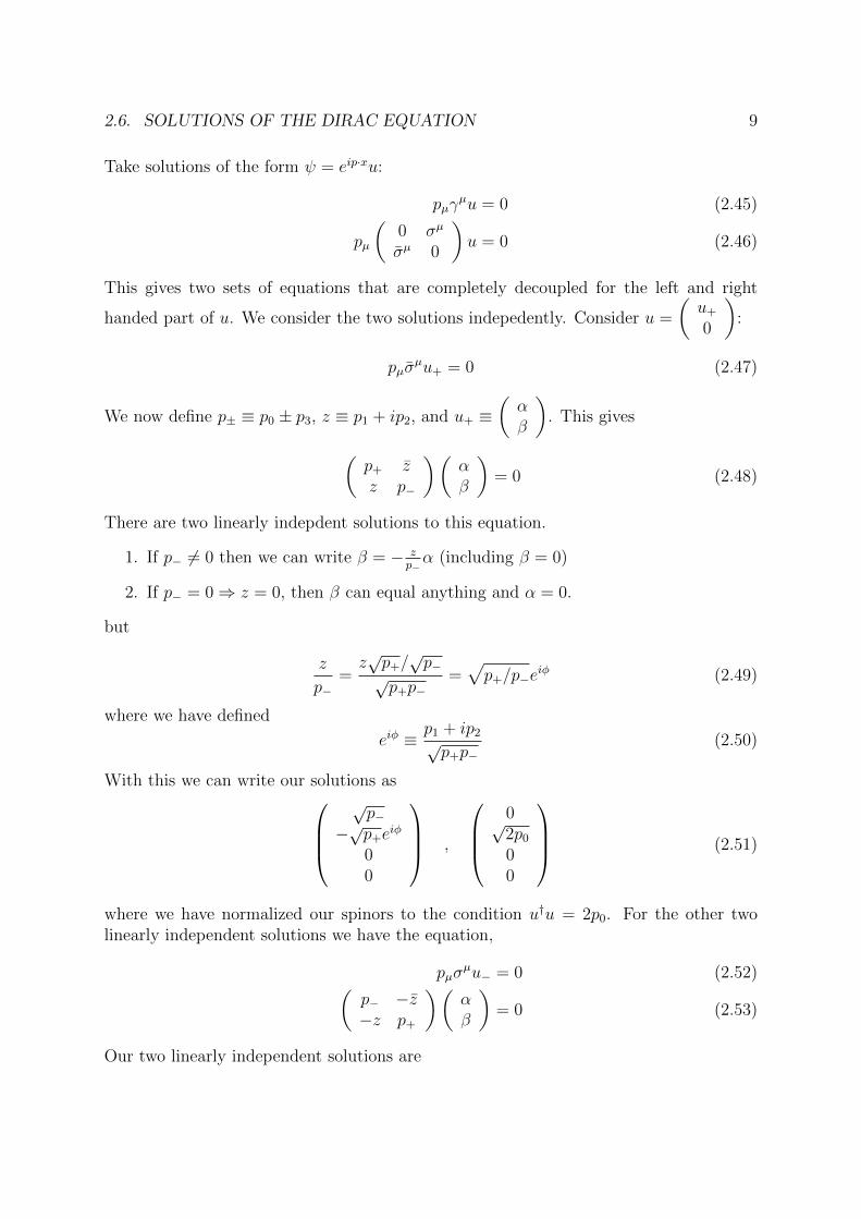
Take solutions of the form ψ = eip·xu:

pµγµu = 0 (2.45)

pµ

(0 σµ

σµ 0

)u = 0 (2.46)

This gives two sets of equations that are completely decoupled for the left and right

handed part of u. We consider the two solutions indepedently. Consider u =

(u+

0

):

pµσµu+ = 0 (2.47)

We now define p± ≡ p0 ± p3, z ≡ p1 + ip2, and u+ ≡(αβ

). This gives

(p+ zz p−

)(αβ

)= 0 (2.48)

There are two linearly indepdent solutions to this equation.

1. If p− 6= 0 then we can write β = − zp−α (including β = 0)

2. If p− = 0⇒ z = 0, then β can equal anything and α = 0.

but

z

p−=z√p+/√p−√

p+p−=√p+/p−e

iφ (2.49)

where we have defined

eiφ ≡ p1 + ip2√p+p−

(2.50)

With this we can write our solutions as√p−

−√p+eiφ

00

,

0√2p0

00

(2.51)

where we have normalized our spinors to the condition u†u = 2p0. For the other twolinearly independent solutions we have the equation,

pµσµu− = 0 (2.52)(

p− −z−z p+

)(αβ

)= 0 (2.53)

Our two linearly independent solutions are


1. If p− 6= 0 then we can write α = (z/p−)β (including α = 0)

2. If p− = 0⇒ z = 0, then α can equal anything and β = 0.

From before we can writez

p−=√p+/p−e

−iφ (2.54)

and 00√

p+e−iφ

√p−

,

00√2p0

0

(2.55)

2.7 Sum Rules

The spin sum formula for the Dirac spinors are given by∑s

usausb = (/p+m)ab (2.56)∑

s

vsavsb = (/p−m)ab (2.57)

The polarization sum rule for external vector bosons is given by

∑λ

εµ(k;λ)εν(k;λ) =

−ηµν (massless boson)

−ηµν + kµkνm2 (massive boson)

(2.58)

Chapter 3

Feynman Rules

3.1 Deriving the Feynman Rules

To properly derive the Feynman rules can be difficult. However determining the interac-tions is easy. The important point is to remember that the Lagrangian is a real scalar.Thus there should generally not be any i’s in it. If there is a complex i then there mustbe an accomadating i somewhere else. Consider an arbitrary interaction:

Lint = g (φn1φm2 ...) (3.1)

where the particular fields in the interaction are irrelevant. Then the Feynman rule forthe interaction will just be

x −→ ig (3.2)

Note that the sign of the terms are conserved. Positive Lagrangian terms give positiveinteraction vertices. Furthermore, there is an i that comes with the term.

Now one subtely is if there is a partial derivative. The proper “replacement” rule forthese is

∂µ → −ipµ (3.3)

where pµ is the momentum of the particle that ∂µ is acting on.

3.2 Symmetry Factors

When using Feynman diagrams to calculate amplitudes a major difficulty in the calcula-tion is to account for identical particles in the calculation. There can be many diagramscorresponding to the exact same process so in general we have to account for all of these.There are 3 contributing factors that result in one factor in front of the amplitude whichis called the Symmetry factor.

1. Each vertex contributes a suppression factor. For example in φ4 theory we typicallyhave a 4! suppression factor for each vertex. Of course the value of these is depen-dent on the definition of the couplings but we define our couplings on purpose sowe end up with symmetry factors on the order of unity.

11

12 CHAPTER 3. FEYNMAN RULES

2. There are different ways external particles can be arranged with each vertex. If youswap all the vertices you get the same diagram.

3. There are equivalent ways to contract the fields in the Wick expansion.

A technique to account for all of these is given by some notes I found online by JacobBourjaily which in turn credits Colin Morningstar [2]. The idea is as follows. Let n bethe number of verteices of a diagram, η be the coupling constant suppression factor, andr the multiplicity of a diagram. Then the Symmetry factor is given by

S =n! (η)n

r(3.4)

and the amplitude is given by

M =1

SM1 diagram (3.5)

The multiplicity of a diagram is the number of different contractions in the Wick expan-sion, or the number of ways to connect all the external lines to the vertices. This canbe found by first drawing out the edges of each external line and points coming out of avertex. Then count the number of ways the lines can be connected.

As an example we consider the “fish” diagram in φ4 theory,

First we draw the edges,

Start with the initial lines. There are eight ways to connect the first line to a vertex.Then since the initial lines and final lines need to be kept as such, there are only 3 waysto connect the second initial line. Continuing on and counting the number of ways eachline can be connected we have

r = (8)(3)(4)(3)(2)(1) (3.6)

This gives a symmetry factor of

S =2! (4!)2

(8)(3)(4)(3)(2)(1)= 2 (3.7)

Chapter 4

Lagrangians and Feynman rules

4.1 Standard Model

The Standard Model charges are summarized below:

doublet T3 = σ3/2 Y Q = T3 + Y2(

νee−

)L

12

−12

−1

−1

0

−1(ud

)L

12

−12

1313

23

−13

singletseR 0 −2 −1uR 0 4

323

dR 0 −23

−13

Higg’s sector(φ+

φ0

) 12

−12

1

1

1

0

4.2 φ4

The Higg’s Lagrangian is given, in my conventions, by,

L = |Dµφ|2 + µ2φ†φ− λ(φ†φ)2 (4.1)

or a potential,V (φ) = −µ2φ†φ+ λ(φ†φ)2 (4.2)

The physical Higgs is given by φ = (0, 1√2(h+ v)). Inserting this into the above I find,

V (h) = −µ2

2(h+ v)2 +

λ

4(h+ v)4 (4.3)

13

14 CHAPTER 4. LAGRANGIANS AND FEYNMAN RULES

The linear term vanishes if v2 = µ2/λ. In this case we can write the potential as,

V (h)− Vmin = λv2h2 + λvh3 +λ

4h4 (4.4)

As always the scalar propagator is

p→ i

p2 −m2h + iε

where, in the normalization above, m2h = 2λv2.

4.3 Spinor QED

af p→Ffb =i(/p+m)ab

p2 −m2 + iε=

(i

/p−m+ iε

)ab

(4.5)

af ←pFfb =i(−/p+m)ab

p2 −m2 + iε=

(i

−/p−m+ iε

)ab

(4.6)

af p→fb =i(−/p+m)ab

p2 −m2 + iε=

(i

−/p−m+ iε

)ab

(4.7)

af ←pfb =i(/p+m)ab

p2 −m2 + iε=

(i

/p−m+ iε

)ab

(4.8)

µg k→ggν = − i

k2 + iε

(gµν − (1− ξ)kµkν

k2

)(4.9)

bgaE

= −ieQ (γµ)ab (+ momentum conservation) (4.10)

(4.11)

where e > 0 and Q = −1 for the electron.

Furthermore, incoming and outgoing photons gives,

µ εµ

µ ε∗µ

4.4. SCALAR QED 15

4.4 Scalar QED

The Lagrangian for scalar QED is given by

L = (Dµφ)†Dµφ−m2φ†φ− λ

4(φ†φ)2 − 1

4FµνF

µν (4.12)

where Dµ = ∂µ − ieQAµ (recall that the negative sign is necessary to give a positivecoupling for the fermion-fermion-vector vertex!). The vertices are given by

Lint = ieQAµ(φ†(∂µφ)− (∂µφ†)φ

)+ e2Q2AµA

µφ†φ− λ

4(φ†φ)2 (4.13)

Depending on the relative directions of the lines going into vertex and the type of particlewe get a different vertex factor. This gives the rule:

φ p→

φ ←p ′

A → ieQ (p+ p′)

and

→ 2ie2Q2gµν

4.5 Electroweak Interactions

The W± ≡ (W1 ∓ iW2)/√

2 boson interactions are given by,

ψi

∂µ−i 12σaWa︷︸︸︷

Dµ γµψ = gψγµ

1

2

(.

√2W+

√2W− .

)ψ + ... =

g√2ψγµPLW

+µ ψ (4.14)

The triple gauge vertices are,


γλ

W−ν

W+µ→ → −ie(gµν(k− − k+)λ − gνλ(q + k−)µ + gλµ(q + k+)ν)

Zλ

W−ν

W+µ→ → −igcW (gµν(k− − k+)λ − gνλ(q + k−)µ + gλµ(q + k+)ν)

The higgs interactions are found through,

φ†(g′

2Y Bµ + gT aW a

µ

)(g′

2Y Bµ + gT bW bµ

)φ (4.15)

=1

4

(. φ0/

√2)†( . .

. 2g2W+W− + (g′Y B − gW3)2

)(.

φ0/√

2

)(4.16)

=g2

4φ2

0W+W− +

e2

4c2W s

2W

φ20

(1

2ZµZ

µ

)(4.17)

which gives a higgs-W+ −W− Lagrangian (there is an additional factor of 2 since eachhiggs in φ0 can get a VEV)1,

W

W

h → ig2v2

Z

Z

h → i e2v2cW sW

The masses of the vector bosons are obtained by taking φ0 → v:

m2W =

g2v2

4, m2

Z =e2v2

4c2W s

2W

(4.18)

The left fermion-Z interactions are derived from,

ψγµ

(g′

2BµY + gT aW aµ

)PLψ = ψγµ

1

2

(g′Y B + gW3 .

. g′Y B − gW3

)PLψ (4.19)

The weinberg angle rotates into the A,Z basis. An angle of 0 corresponds to hyperchargebeing fully aligned with charge (i.e., Bµ = Aµ):(

Bµ

W 3µ

)=

(cW −sWsW cW

)(AµZµ

)(4.20)

1We take φ0 = h+ v such that v ' 246GeV .

4.5. ELECTROWEAK INTERACTIONS 17

and the couplings are related to the electroweak couplings by,

|e| = g′cW = gsW |e| =√g′2 + g2 (4.21)

and in our conventions,

Q = T3 +Y

2(4.22)

This corresponds to,

g′Y Bµ ± gW 3µ = e

(Y ± 1)Aµ +

1

sW cW

(±1 + s2

W (−Y ∓ 1))Zµ

(4.23)

The up-type and down-type fermion interactions are,

Lup−typeNC =

eQAµ +

e

cW sW

(1

2−Qs2

W

)Zµ

uγµPLu (4.24)

Ldown−typeNC =

eQAµ −

e

cW sW

(1

2+Qs2

W

)Zµ

dγµPLd (4.25)

The right handed couplings are

LψRψRZ + ... = ψγµg′BµQPRψ = −eQsW

cWψγµPRψZ

µ + ... (4.26)

We now compute the interactions of the goldstones with the vector bosons. Thesearise from the higgs kinetic term:

(DµH)†DµH =(

(∂µ − igT aW aµ − i

g

2Bµ)H

)†((∂µ − igT aW a

µ − ig′

2Bµ)H

)(4.27)

= |∂µH|2 + ∂µH†(−igT aW a

µ − ig′1

2Bµ

)H +H†

(igT aW a

µ + ig′

2Bµ

)∂µH

+

∣∣∣∣(gT aW aµ +

g′

2Bµ

)H

∣∣∣∣2 (4.28)

= |∂µH|2 −i

2

[∂µH

†(gW + g′B g

√2W+

√2gW− −gW 3 + g′B

)µH −H† (...)µ ∂

µH

]+

1

4H† (...)µ (...)µH (4.29)

The first term is just a kinetic term. We first simply the term in square brackets.

[...] = ∂µ

(π− 1√

2(h− iπ0)

)( gW + g′B g√

2W+√

2gW− −gW 3 + g′B

)µ(π+

1√2

(h+ iπ0)

)− h.c.

(4.30)


• π0π0Z:

− gW 3 + g′B = − e

swcwZ (4.31)

⇒∆L = −1

2

e

swcw

[(∂µπ

0)π0Zµ −

(∂µπ

0)π0Zµ

]= 0 (4.32)

Thus there is not π0π0Zµ interaction. This is comforting as the SM doesn’t have atriple-Z interaction. This can be traced back to the fact that the Goldstones form atriplet of SU(2)L and so the interactions are parameterized by, εabcWaWbWc whichdoesn’t have a ZZZ interaction from the structure of the Levi-Cevita tensor.

• hπ0Z:

∆L = −1

2

e

swcwi[(∂µh)π0Zµ − h

(∂µπ

0)Zµ]− h.c. = −i e

swcw

[∂µ(hπ0)Zµ

](4.33)

• hhZ:

∆L = −1

2

e

swcw(∂µh)hZµ − h.c. = 0 (4.34)

• π−π+Z, π−π+A:

∆L = (∂µπ−)π+

(gW 3 + g′B

)µ − h.c. (4.35)

= e[(∂µπ

−)π+](

2Aµ +1

swcw

(1− 2s2

w

)Zµ

)− h.c. (4.36)

• π±W∓h:

∆L = g(∂µπ

−)W+µh+ g (∂µh) π+W−µ − h.c. (4.37)

= gh(∂µπ

+W+µ − ∂µπ+W−µ)+ g (∂µh)[π−W+µ − π+W−µ] (4.38)

= g[∂µ(hπ−)W+µ

]− h.c. (4.39)

Now lets consider the terms arising from the∣∣H† (...)2H

∣∣2 term. We have,

|...|2 =1

4H†(

a2 + 2g2W−µ W

± g√

2(a+ b) ·W+

g√

2(a+ b) ·W+ b2 + 2g2W+ ·W−

)H (4.40)

where aµ ≡ e(

2Aµ + 1swcw

(1− 2s2w)Zµ

)and bµ = − e

cwswZµ. The terms arising from this

contribution are given below:

• π+π−, A, Z,W :

∆L =e2

4π+π−

[(2Aµ +

1

swcw

(1− 2s2

w

)Zµ

)2

+ 2g2W+µ W

−µ

](4.41)

4.6. YUKAWA COUPLINGS 19

• (π0)2, h2,W 2, Z2:

∆L =1

4

1

2

(h2 + π0 2

) [( e

swcw

)2

ZµZµ + 2g2W+

µ W−µ

](4.42)

• π−(h, π0)Z,W+: Top right:

∆L =1

4π−(h+ iπ0

) (g(a+ b) ·W+µ

)(4.43)

=e2

2

[(h+ iπ0

)π− (Aµ − twZµ)W+µ

](4.44)

The bottom left contribution is similar. The sum gives,

e2

2

[(Aµ − twZµ)

((h+ iπ0)π−W+µ +

(h− iπ0

)π+W−µ)] (4.45)

4.6 Yukawa couplings

The yukawa interactions are given by,

Lyuk = −yijd QiL,0φd

jR − y

iju (Qi

L,0εφ)ujR + h.c. (4.46)

where QL,0 is the field prior to rotation to the physical basis (the right-handed fields arealready implicitly rotated and absorbed into the yukawa couplings). The different termscan be rewritten:

uiL ≡ U iju u

jL,0 diL ≡ U ij

d dL,0 (4.47)

Vij ≡ (U †uUd)ij (4.48)

mu = U †uyuv√

2 md ≡ U †dvyd√

2 (4.49)

Then we can write,

Lyuk = −g/√

2

mW

((V md)

ji uiL djL)( π+

(h+ iπ0)/√

2

)dR,j

+(ujL (V †mu)

jidiL)ij

((h− iπ0)/

√2

−π−)uR,j

+ h.c. (4.50)

where its understood that the mass matrices are diagonal. From here we can read off theFeynman rules. Here we check one entry with the literature:

L ⊃ g√2V †jk

mu,ki

mW

diLujRπ− + h.c. (4.51)

This is in agreement with the Feynman rules displayed in [4]


4.7 CKM Matrix

The CKM matrix in the Wolfenstein parametrization is

VCKM =

1− λ2

2λ Aλ3(ρ− iη)

−λ 1− λ2

2Aλ2

Aλ3(1− ρ− iη) −Aλ2 1

(4.52)

4.8 Supersymmetry

In this section we summarize the supersymmetric Feynman rules for a gauge theory.We continue to take the Peskin and Schroeder convention for the sign in the covariantderivatives. This comes at the come of deviating from the convention used in Martin’snotes by a minus sign for the gauge charge. For a field charged under a gauge group theD term is given by, ∫

d4θΦ†eV Φ = iψ†σµDµψ +√

2g(φ†T aψ)λa + ... (4.53)

It is often useful to have the form of this expression in the case of a field charged underSU(2) × U(1). We denote the field by uL, dL but they refer to up-type and down-typefields respectfully. We have,∫

d4θΦ†eV Φ =√

2g(φ†T aψ

)W a +

√2g′

Y

2φ†Bψ + h.c.+ ... (4.54)

=(u†L d†L

) 1√2

(gW0 + Y gB

√2gW+

√2gW− g′Y B − gW0

)(uLdL

)+ h.c. (4.55)

= u†L1√2

(gW0 + Y gB

)uL + d†L

1√2

(gY B − gW0

)dL + g

(u†LW

+dL + d†LW−uL

)(4.56)

4.8.1 Triplet

Above we considered the additional EW interactions for a field in the fundamental rep-resentation. Now we extend this to fields in the adjoint representation. For an adjointfield we have the new interactions,

√2g(φ†T aψ

)W a + gψ†Taσ

µψW aµ (4.57)

There are no additional B terms since fields in the adjoint representation of a U(1) aren’tcharged under the group. We start by considering the first term. Using T abc = ifabc = iεabcwe have,√

2g(φ†T aψ

)W a =

√2igφ†bεbacψcW

a (4.58)

=√

2g(φ†1 φ†2 φ†3

) 0 −W 3 W 2

W 3 0 −W 1

−W 2 W 1 0

ψ1

ψ2

ψ3

(4.59)

4.8. SUPERSYMMETRY 21

We want to write the fields according to their charged basis. For this we use the trans-formations,(

ψ−ψ+

)=

1√2

(1 +i1 −i

)(ψ1

ψ2

) (φ−φ+

)=

1√2

(1 +i1 −i

)(φ1

φ2

)(4.60)

We define,

U ≡ 1√2

1 i 01 −i 00 0 1

(4.61)

and so,

i√

2g(φ†− φ†+ φ†0

)UAU †

ψ−ψ+

ψ0

(4.62)

where,

A ≡

0 −W 0 − i√

2(W− − W+)

W 0 0 −12

(W− + W+

)i√2

(W− − W+

)1√2

(W− + W+

)0

(4.63)

Multiplying through gives,

−√

2g(φ†− φ†+ φ†0

) W 0 0 −W−

0 −W 0 W+

−W+ W− 0

ψ−ψ+

ψ0

(4.64)

The simpilfication for the second term is identical with g → g/√

2, φ → ψ, andW → W ,

gψ†TaσµψW a

µ = −g(ψ†− ψ†+ ψ†0

) W 0µ 0 −W−

µ

0 −W 0µ W+

µ

−W+µ W−

µ 0

σµ

ψ−ψ+

ψ0

(4.65)

To rewrite this in terms on the physical gauge bosons we use, W 0µ = sWAµ + cWZµ.

Chapter 5

Polarized Calculations

5.1 Polarization and Spin

For some reason a thorough discussion of polarization calculations is missing from thepopular Quantum Field Theory books. The discussion here is an amalgam of what I’vefound from Peskin, Srednicki, as well as Bjorken and Drell.

Consider a particle with a spinor u(p, s) or v(p, s) which is at rest. It’s polarization inthe rest from of the particle is what we often call its spin. We denote this polarization assome 3-vector λ. For example if the particle is polarized along the z axis then λ = (0, 0, 1).We form a four-vector to represent its “spin”. We denote the rest frame spin vector bysµr . Now what should the first component of the four-vector be? In the rest frame thereis no other degree of freedom for the spin. We set s0

r to zero.

To boost back to the lab frame we apply a Lorentz Transformation in the −p directiononto the four-vector. Recall in matrix form the transformation matrices applied onto avector (t, r):

t′ = γ (t− r · v) (5.1)

r′ = r +

(γ − 1

v2r · v − γt

)v (5.2)

22

5.1. POLARIZATION AND SPIN 23

The spatial component of the spin in the lab frame is

s = λ +

(−γ − 1

v2λ · v − 0

)(−v)

= λ +

(γλ · (γmv)

mγ− λ · γmv

γm

)vγm

= λ +

((γ − 1)λ · pE2(γ2 − 1)

γ2

)p

= λ +p(λ · p)

E2m(E +m)E2

= λ +p(λ · p)

m(E +m)(5.3)

and the time component is

s0 = γλ · vm/m

=p · λm

(5.4)

So we have

sµ =

(p · λm

,λ +p(p · λ)

m(m+ E)

)(5.5)

In the case that the spin is measured along the direction of motion (i.e. p ‖ λ) we have

sµ =1

m(|p| , pE) (5.6)

Note that

s2 =(p · λ)2

m2− λ2 − 2

(p · λ)2

m(E +m)− p2(p · λ)2

m(m+ E)

= (p · λ)2

(1

m2− 2

m(E +m)− E2 −m2

m2(m+ E)2

)− 1

= (p · λ)2

(E2 + 2mE +m2 − 2Em− 2m2 − E2 +m2

m2(E +m)2

)− 1

= −1 (5.7)

and

sµpµ =

p · λEm

− p · λ− (E2 −m2)(p · λ)

m(m+ E)

= (p · λ)

(E

m− 1− E −m

m

)= (p · λ)

E −m− E +m

m= 0 (5.8)

24 CHAPTER 5. POLARIZED CALCULATIONS

For a general spin vector the spin projection operator is (see for example [1])

Σ(s) =1 + γ/s

2(5.9)

This operator obeys

Σ(s)u(p, s) = u(p, s) (5.10)

Σ(s)v(p, s) = v(p, s) (5.11)

Σ(−s)u(p, s) = Σ(−s)v(p, s) = 0 (5.12)

5.2 Calculational Tricks

When doing a calculation with some polarized particles there are some useful tricks thatcan be implemented to simplify the math. The key result that can be used to derive allthe following relations is

u(p,λ)u(p,λ) =(/p+m

)Spin Projection Operator︷︸︸︷1 + γ5/s

2(5.13)

v(p,λ)v(p,λ) =(/p−m

) 1 + γ5/s

2(5.14)

With this we can now find a variety of important relations (we suppress the polariza-tion and momentum dependence in u:

uγµu = tr (uγµu)

= tr (γµuu)

=1

2tr(γµ(/p+m

) (1 + γ5/s

))=

1

2tr(γµ/p)

= 2pµ (5.15)

uγµγ5u = tr(uγµγ5u

)= tr

(γµγ5uu

)=

1

2tr(γµγ5

(/p+m

) (1 + γ5/s

))=

1

2tr (+mγµ/s)

= 2msµ (5.16)

Chapter 6

Renormalization

Renormalization schemes is subtle topic with a lot of depth. Here we just present thebare-bones needed to do calculations

6.1 On-Shell Renormalization

There are two renormalization conditions to consider. First corresponds to the massrenormalization. Consider the full particle propagator (with the external lines amputated,i.e. ignore the external legs contribution):

p→FFp→+

p→FpFp→+

p→FxxxxxxxxxxxxxFp→(6.1)

whereFpF represents a sum of loop corrections andFxxxxxxxxxxxxxF is the counterterm.It can be shown that the Green function corresponding the above computation are (inthe case of φ− 4 theory)

〈Ω|φ(x)φ(y)|Ω〉 =i

p2 −m2p + Σ(p2) + iε

(6.2)

where Σ(p2) is the sum of the amputated diagrams above. There are two shift factorshere. There is a shift in the pole and there is a also a shift in the amplitude of thisfactor. The first renormalization condition is that when the incoming particle is on-shell(p2 = m2

p), the loop contribution (Σ) is zero. In other words(p→FpFp→

+p→FxxxxxxxxxxxxxFp→

) ∣∣∣∣p2=m2

p

= 0 (6.3)

This makes sence sinceFF should give the propagator for an on-shell particle.

The second renormalization condition is for the normalization of the Green’s function

25

26 CHAPTER 6. RENORMALIZATION

not to change. We can rewrite equation as

〈Ω|φ(x)φ(y)|Ω〉 =i

p2 −m2p + Σ(m2) + (p2 −m2) dΣ

dp2

∣∣∣∣p2=mp

+ iε

(6.4)

=i

(p2 −m2p)

(1 + dΣ

dp2

∣∣∣∣p2=mp

)+ Σ(m2) + iε

(6.5)

(6.6)

where we only keep terms of order p2 −m2 since we are considering the conditions on Σnear the pole (these are on-shell conditions after all!). Thus we require (in φ− 4 theory):

dΣ

dp2

∣∣∣∣p2=m2

= 0 (6.7)

The third renormalization condition is for the coupling. The sum of the 4 vertexdiagrams (this can of course be done for any types of couplings but we consider 4 externallegs for concreteness).

DE

+ DpE

+DxxxxxxxxxxxxxE

(6.8)

The renormalization condition is DpE

+DxxxxxxxxxxxxxE

∣∣∣∣s+u+t=4m2

= 0 (6.9)

where λ is the renormalized couplings.

Chapter 7

Quantum Mechanics

7.1 Commutation Relations

[x, p] = i~ (7.1)

7.2 Quantum Harmonic Oscillator

The creation annhillation operators are defined by

a ≡ mω

2~

(x+

i

mωp

)(7.2)

a† =√mω2~

(x− i

mωp

)(7.3)

or

x =

√~

2mω(a+ a†) (7.4)

p = i√mω~2(a† − a) (7.5)

which give

a† |n〉 =√n+ 1 |n+ 1〉 (7.6)

a |n〉 =√n |n− 1〉 (7.7)

We also have,〈0|ana†n|0〉 = n! (7.8)

This is easiest to see by starting with n = 1 and going on recursively to higher n.

27

Chapter 8

Special Relativity

In special relativity we have covariant (xµ) and contravariant (xµ) vectors. Contravariantvectors have positive spatial indices:

xµ = (x0,x) (8.1)

while covariant vectors have negative spatial indices:

xµ = (x0,−x) (8.2)

The derivatives have the opposite sign convention,

∂µ ≡ (∂0,∇) (8.3)

∂µ ≡ (∂0,−∇) (8.4)

28

Chapter 9

Phase space

The differential cross section of a two-body collision is given by,

dσ =1

2EA2EB |vA − vB|

∫dΠ |M|2 (9.1)

where Ei and vi are the incoming particle energies and velocities, while we define,

dΠ ≡

(∏f

d3pf(2π)3

1

2Ef

)(2π)4δ(4)(

∑i

pi −∑f

pf ) (9.2)

If the incoming particles are identical particles we have, EA = EB = Ecm/2, and vA −vB = 2 |pi| /Ecm, which gives,

dσ =1

8Ecm |pi|

∫dΠ |M|2 (9.3)

where pi is the momenta of the incoming particles.The differential decay rate is,

dΓ =1

2mA

∫dΠ |M|2 (9.4)

For a two particle final state the phase space is just,∫dΠ2 =

∫dΩcm

4π

1

8π

2 |p|Ecm

(9.5)

where |p| is the magnitude of the momentum of either outgoing particle (they are equalin the cm frame), and Ecm =

√s is the cm energy. In the massless limit this is just, [Q

1: There is factor of 2 problem floating around....]∫dΠ2 =

1

8π

∫dΩcm

4π(9.6)

29

30 CHAPTER 9. PHASE SPACE

Finally for 2→ 2 process with all massless particles we have,

dσ =1

8πs

∫dΩcm

4π|M|2 (9.7)

If we have a 2→ 2 process with the outgoing particles having equal mass then we canrewrite the phase space as,

1

4πs

∫ − s4

(1−β)2

− s4

(1+β)2dt (9.8)

where β ≡√

1− 4m2

sand t is the Mandelstam variable. In the massless limit this takes

the form,1

4πs

∫ 0

−sdt (9.9)

The three particle phase space for unpolarized particles with two massless particles(i = 1, 2) and one massive (i = 3) is,∫

dΠ3 =s

128π3

∫ 1−α2

0

dx1

∫ 1−(α2/(1−x1))

1−α2−x1dx2 (9.10)

where α ≡ m3/√s, s ≡ (

∑pi)

2, and xi ≡ 2Ei/√s is the momentum fraction of particle

i. For m3 → 0 we have the better known result,∫dΠ3 =

s

128π3

∫ 1

0

dx1

∫ 1

1−x1dx2 (9.11)

Chapter 10

Mathematics

10.1 Anticommuting Matrices

10.1.1 Sigma Matrices and Levi Civita Tensors

σ1 =

(0 11 0

)σ2 =

(0 −ii 0

)σ3 =

(1 00 −1

)(10.1)

They obey the commutation relations,

[σa, σb] = 2iεabcσc (10.2)

and the anticommutation relations,

σa, σb = 2δab (10.3)

Furthermore any product of Pauli matrices can be written as

σaσb = iεabcσc + δab (10.4)

They also obey,

σ2i = 1 (10.5)

(σa)∗ = iσ2σaiσ2 (10.6)

Trσi = 0 (10.7)

detσi = −1 (10.8)

It is a common practice to exponentiate a linear combination of these matrices. Wederive the general formula below,

eiθiσi = 1 + iθiσi −1

2θiθjσiσj − ... (10.9)

=

(1− 1

2(θiσi)

2 + ...

)+ i

(θiσi −

1

3!(θiσi)

3 + ...

)(10.10)

31

32 CHAPTER 10. MATHEMATICS

but

θiθj(σiσj) = θiθj(iεijkσk + δij) (10.11)

= θ2 (10.12)

and

(θiσi)3 = θ2θiσi (10.13)

so

eiθiσi = cos θ + iθiσiθ

sin θ (10.14)

σµσν + σν σµ = 2ηµν (10.15)

We also have

tr σµσν = 2ηµν (10.16)

(σµ)αα(σµ)ββ = 2δ βα δ β

α (10.17)

Furthremore,

σµν =1

2iεµνρσσρσ (10.18)

We have

ε0123 = −ε0123 = +1 (10.19)

and

εijkεimn = δmj δ

nk − δnj δmk (10.20)

εjmnεimn = 2δij (10.21)

εijεin = δnh (10.22)

Furthermore, we have

εσµνρεσαβγ = 6δ[µα δ

νβδ

ρ]γ (10.23)

εµνρσερσαβ = −4δ[µα δ

ν]β ≡ −4

(δµαδ

νβ − δναδνβ

)(10.24)

where the square brackets denote all possible permutations of µ, ν, ρ. Each permutationhas a negative sign if it is an odd permutation.

The three dimensional extension of the Pauli matrices are:

1√2

0 1 01 0 10 1 0

,1√2

0 −i 0i 0 −i0 i 0

,

1 0 00 0 00 0 −1

(10.25)

10.1. ANTICOMMUTING MATRICES 33

10.1.2 Gamma Matrices

In the Weyl basis the Gamma matrices can be written

γµ =

(0 σµ

σµ 0

)(10.26)

where σµ = 1,σ and σµ = 1,−σ. They obey the defining commutation relation

γµ, γν = 2gµν (10.27)

This leads to many important relations. For example

γµγµ =1

2γµγµ + γµγµ (10.28)

=1

2

2gµµ

(10.29)

= 4 (10.30)

γµγαγµ = γµ(2gαµ − γµγα

)(10.31)

= 2γα − 4γα (10.32)

= −2γα (10.33)

In the Weyl basis the Gamma-5 matrix takes the form

γ5 =

(−1 00 1

)(10.34)

and has the properties that

(γ5)† = γ5 (10.35)

(γ5)2 = 1 (10.36)γ5, γµ

= 0 (10.37)

The γ5 matrix can be used to form projection operators:

PL =1− γ5

2(10.38)

PR =1 + γ5

2(10.39)

Furthermore we have,/a/b = a · b− iaµσµνbν (10.40)

and in particular,/a/a = a2 (10.41)


Trace Technology

(uγµv)∗ = v†γµ† (10.42)

= vγ0γµ†γ0u (10.43)

= vγ0(γ0γµγ0)γ0u (10.44)

(uγµv)∗ = vγµu (10.45)

We have

tr (γµγν) =1

2tr (γµγν + γµγν) (10.46)

=1

2tr (γµγν + 2ηµν − γνγµ) (10.47)

=1

2tr (γµγν + 2ηµν − γµγν) (10.48)

=1

2tr (2ηµν) (10.49)

= 4ηµν (10.50)

where we have used the cyclic property of traces.

Furthermore we have

tr(γ5)

= 0 (10.51)

tr(γµγνγ5

)= 0 (10.52)

tr(γµγνγργσγ5

)= −4iεµνρσ (10.53)

10.2 Complete the Square

To complete the square we want to take an expression of the form ax2 + bx + c tod(x+ e)2 + f . Expanding the second form gives

dx2 + 2dex+ de2 + f (10.54)

first off, clearly a = d. So we make the identifications, b = 2ae, ae2 + f = c. However, wetypically want the inverted form of these equations. So we have

d = a (10.55)

e =b

2a(10.56)

f = c− b2

4a(10.57)

10.3. DEGREES OF FREEDOM IN A MATRIX 35

10.3 Degrees of Freedom in a Matrix

The number of degrees of freedom in a unitary matrix are found below. The number offree parameters in a general complex matrix is 2N2. Unitarity implies that U †U = 1. Wedefine the elements of U as aij + ibij. Then unitarity implies

(aij + ibij)(aji − ibji) = δij (10.58)

which gives two equations,

aijaji + bijbji = δij (10.59)

bijaji − aijbji = 0 (10.60)

The first equation is symmetric under interchanging i↔ j and gives

1 + 2 + ...+N =N(N + 1)

2(10.61)

conditions (just think of it as a matrix equation and the independent equations makingup a top right triangle of the matrix).

The second equation is antisymmetric under changing i↔ j (the component of i = jvanishes trivially as doesn’t offer an extra constraint). This gives

1 + 2 + ...+N − 1 =N(N − 1)

2(10.62)

conditions.

Thus the number of free parameters in a Unitary matrix is

2N2 −N2 = N2 (10.63)

10.4 Feynman Parameters

Two denometers can be combined as

1

AB=

∫ 1

0

dx1

[xA+ (1− x)B]2(10.64)

n denomenators can be combined as

1

A1A2...An=

∫ 1

0

dx1 dx2... dxnδ(∑i

xi − 1)(n− 1)!

[x1A1 + ...+ xnAn]n(10.65)


This is done below for a common two denomenators:

1

(`− p)2 −m21 + iε

1

`2 −m22 + iε

=

∫dx

1

[x((`− p)2 −m21 + iε) + (1− x)(`2 −m2

2 + iε)]2

=

∫dx

1

[`2 − 2`px+ p2x+ (m22 −m2

1)x−m22 + iε]

2

=

∫dx

1

[(`− px)2 + p2x(1− x) + (m22 −m2

1)x−m22 + iε]

2

=

∫dx

1

[(`− px)2 −∆ + iε]2(10.66)

where we have defined ∆ ≡ −p2x(1− x) + (m21 −m2

2)x+m22.

10.5 n - sphere

The surface area of a unit n− sphere is

Sn = (n+ 1)π(n+1)/2

Γ(n+1

2+ 1) (10.67)

Note in this notation a sphere in our 3D world corresponds to S2 = 4π.

10.6 Integrals

10.6.1 Sample Loop Integral

One common integral (usually in φ− 4 theory) is the following∫d4`

1

`2 −∆ + iε(10.68)

We perform this integral here to refer to this result in the future. We assume φ− 4 so wecan work with the cutoff. The integral can be split as follows

=

∫d3`d`0

1

`20 − `2 −∆ + iε

The poles are at

`20 − `2 −∆ + iε = 0

`0 = ±(√

`2 + ∆− iε)

The positions of the poles are shown below

10.6. INTEGRALS 37

Re(`0)

Im(`0)

××

We can apply a Wick rotation such that `0 → i`0. This gives

= i

∫d3`d`0

1

−`20 − `2 −∆ + iε

= −i∫d4È

1

`2E + ∆

where we define a Eulidean four vector, È = (`0, ì) with `2E ≡ `2

0 + `2i . Since we are now

far from the poles we also omit the iε factors.

= −i2π2

∫dÈ

`3E

`2E + ∆

= −i2π2

∆

∫ Λ

0

∆1/2 dx∆3/2x3

x2 + 1

= −i2π2∆

∫ Λ/m

0

dxx3

x2 + 1

= −iπ2∆

(Λ2

∆− log

(1 + Λ2/∆

))= −iπ2

(Λ2 −∆ log

(∆ + Λ2

∆

))(10.69)

10.6.2 Dimensional Regularization and the Gamma Function

There are two particularly useful integrals when using dim-reg([3], pg. 251):∫ddÈ(2π)d

1

(`2E + ∆)n

=1

(4π)d/2Γ(n− d

2

)Γ(n)

∆d/2−n (10.70)∫ddÈ(2π)d

`2E

(`2E + ∆)2

=1

(4π)d/2d

2

Γ(n− d

2− 1)

Γ(n)∆d/2−n+1 (10.71)

The Gamma function is the generalization of the factorial. It obeys the relationships

Γ(n) = (n− 1)! , (10.72)


Γ(n+ 1) = nΓ(n) , (10.73)

and

Γ

(1

2

)=√π (10.74)

When using “dim reg” to regular your integrals it is often useful to expand Γ(ε) to firstorder:

Γ(ε) =1

ε− γ +

1

12(6γ2 + π2)ε+O(ε2) (10.75)

Γ(−1 + ε) = −1

ε+ (γ − 1) (10.76)

where γ ≈ 0.577.To expand any other terms of the form ∆ε one can use

∆ε = elog ∆ε

(10.77)

= eε log ∆

= 1 + ε log ∆ (10.78)

We can use symmetry in the integrals to replace,

`µ`ν → 1

d`2gµν (10.79)

`µ`ν`ρ`σ → 1

d(d+ 2)(`2)2(gµνgρσ + gµρgνσ + gµσgνρ) (10.80)

10.6.3 d-dimensional integrals in Minkowski space

∫dd`

(2π)d1

(`2 −∆)n=

(−1)ni

(4π)d/2Γ(n− d

2

)Γ(n)

(1

∆

)n− d2

(10.81)∫dd`

(2π)d`2

(`2 −∆)n=

(−1)n−1i

(4π)d/2d

2

Γ(n− d

2− 1)

Γ(n)

(1

∆

)n− d2−1

(10.82)∫dd`

(2π)d`µ`ν

(`2 −∆)n=

(−1)n−1i

(4π)d/2gµν

2

Γ(n− d

2− 1)

Γ(n)

(1

∆

)n− d2−1

(10.83)∫dd`

(2π)d(`2)2

(`2 −∆)n=

(−1)ni

(4π)d/2d/(d+ 2)

4

Γ(n− d

2− 2)

Γ(n)

(1

∆

)n− d2−2

(10.84)∫dd`

(2π)d`µ`ν`ρ`σ

(`2 −∆)n=

(−1)ni

(4π)d/2Γ(n− d

2− 2)

Γ(n)

(1

∆

)n− d2−2

× 1

4(gµνgρσ + gµρgνσ + gµσgνρ)

(10.85)

Bibliography

[1] J. Bjorken and S. Drell. Relativistic quantum mechanics. McGraw-Hill, 1964.

[2] J. Bourjaily. Physics 513, quantum field theory - homework 7. http://www-personal.umich.edu/ jbourj/qft.htm, 2013.

[3] M. Peskin and D. Schroeder. An Introduction to Quantum Field Theory. West ViewPress, 1995.

[4] J. C. Romao and J. P. Silva. A resource for signs and Feynman diagrams of theStandard Model. Int. J. Mod. Phys., A27:1230025, 2012.

39

useful relations in quantum field...

Documents