use of west virginia permanent traffic recorder data to

Graduate Theses, Dissertations, and Problem Reports

2002

Use of West Virginia permanent traffic recorder data to develop Use of West Virginia permanent traffic recorder data to develop

factors for traffic and truck variation factors for traffic and truck variation

Jacob Scott D'Angelo West Virginia University

Follow this and additional works at: https://researchrepository.wvu.edu/etd

Recommended Citation Recommended Citation D'Angelo, Jacob Scott, "Use of West Virginia permanent traffic recorder data to develop factors for traffic and truck variation" (2002). Graduate Theses, Dissertations, and Problem Reports. 1224. https://researchrepository.wvu.edu/etd/1224

This Thesis is protected by copyright and/or related rights. It has been brought to you by the The Research Repository @ WVU with permission from the rights-holder(s). You are free to use this Thesis in any way that is permitted by the copyright and related rights legislation that applies to your use. For other uses you must obtain permission from the rights-holder(s) directly, unless additional rights are indicated by a Creative Commons license in the record and/ or on the work itself. This Thesis has been accepted for inclusion in WVU Graduate Theses, Dissertations, and Problem Reports collection by an authorized administrator of The Research Repository @ WVU. For more information, please contact [email protected].

https://researchrepository.wvu.edu/

https://researchrepository.wvu.edu/

https://researchrepository.wvu.edu/etd

https://researchrepository.wvu.edu/etd?utm_source=researchrepository.wvu.edu%2Fetd%2F1224&utm_medium=PDF&utm_campaign=PDFCoverPages

https://researchrepository.wvu.edu/etd/1224?utm_source=researchrepository.wvu.edu%2Fetd%2F1224&utm_medium=PDF&utm_campaign=PDFCoverPages

mailto:[email protected]

Use of West Virginia Permanent Traffic Recorder Data to DevelopFactors for Traffic and Truck Variation

By

Jacob S. D’Angelo

Thesis submitted to theCollege of Engineering and Mineral Resources

at West Virginia Universityin partial fulfillment of the requirements

for the degree of

Master of Sciencein

Civil Engineering

Ronald W. Eck, Ph.D., ChairLloyd James French III, Ph.D.

Darrell R. Dean, Ph.D.

Department of Civil and Environmental Engineering

Morgantown, West Virginia2002

Keywords: Traffic Monitoring, Axle Correction Factors, Peak Hour Volume,Design Hour Volume, and Truck Factors

The purpose of this study was to use data collected from the 52 permanent count stations

located throughout the state to develop four sets of factors that would assist the West

Virginia Department of Transportation (WVDOT) in the management and engineering of

the roadways in West Virginia.

The objectives of this study were to:

1) Establish correction factors that can be applied to the short-term single

pneumatic tube traffic count stations to adjust for the effect of three or more

axle trucks on the volume counts.

2) Establish factors that use the peak hour volume (PHV) to estimate the design

hour volume (DHV).

3) Establish factors that relate the percentage of trucks in the average daily traffic

(ADT) to a) the percentage of trucks in the peak hour and b) the percentage of

trucks in the hours used by the WVDOH in conducting manual classification

counts.

Using analysis of variance (ANOVA analysis) to determine statistical significance, the

factors were approximately aggregated and either reported by year, month of the year,

quarter, or day of the month. The axle correction factors were reported by functional

class by year, except rural interstates. Due to a significant difference in the first quarter,

one factor was reported for the first quarter and another factor was reported for the rest of

the year. PHV to DHV factors were reported by day of the month for each functional

classification. The factors relating percent of trucks in the ADT to a) the percentage of

trucks in the peak hour and b) the percentage of trucks in the hours used by the WVDOH

in conducting manual classification counts were reported by rural heavy truck route,

urban heavy truck route, or “other” routes due to the insignificant variability within the

normal functional class groupings. The only variability detected was between the

interstates and the non-interstate roadways. The detailed tables containing these factors

are presented in the report.

iii

VITA

The author, Jacob D’Angelo, was born April 16, 1979 in Parkersburg, West Virginia,

where he lived until moving to Elkins, West Virginia at the age of 11. The author

graduated from Elkins High School in the spring of 1997 and was accepted to attend

West Virginia University in the fall of 1997. Graduating magna cum laude, Jacob

received his bachelor’s degree in Civil and Environmental Engineering in the spring of

2001. The author was then accepted to attend graduate school at West Virginia

University, specializing in the transportation field of civil engineering. By completing

graduate-level courses while finishing his master’s degree, his course requirements for a

master’s degree were met in December 2001.

iv

ACKNOWLEDGEMENTS

The author would like to thank the West Virginia Division of Highways for their

financial support of this project. The interest and continued technical support throughout

the duration of this research project provided by Jerry Legg is sincerely appreciated.

Also, a word of thanks to the Department of Civil and Environmental Engineering at

West Virginia University for the opportunity to continue my education and broaden my

knowledge in the field of Civil Engineering. The author would like to thank the faculty

and staff of the CEE department, with a special thanks to Dr. Ronald Eck, Dr. Jim

French, and Dr. Darrell Dean for their guidance throughout this research project.

v

TABLE OF CONTENTS

PageABSTRACT…………………………………………………………………………… ii

VITA……………………………………………………………………………………iii

ACKNOWLEDGEMENTS………………………………………………..………….. iv

TABLE OF CONTENTS……………………………………………….………………v

LIST OF TABLES……………………………………………...………………………vii

LIST OF FIGURES…………………………………..………………………………... ix

Chapter 1

INTRODUCTION…………………………………………..…………………………… 1

1.1 Background…………………………………………………………………..11.2 Problem Statement………………………………………………………….. 41.3 Project Objectives……………………………………………………………71.4 Organization of Report…………………………………………….……….. 7

Chapter 2

LITERATURE REVIEW……………………………………………………………….. 8

2.1 Introduction………………………………………………………………….82.2 Traffic Monitoring Programs…………………………………………….….9

a. Procedure Guidelines…………………………………………………9b. Permanent and Short-Term Counts………………………………… 10c. Error-Checking Methodologies……………………………………. 12

2.3 Developing Axle Correction Factors Using Vehicle Classification Counts..14

a. Overview…………………………………………………………… 14b. Determination of Axle Adjustment Factors………………………... 15c. Grouping the Data Collection Sites………………………………... 17d. Variation of Factors with Time…………………………………….. 20

2.4 Percentage of Trucks in Traffic Stream…………………………………... 252.5 Relationship of Design Hour Volume and Peak Hour Volume…………... 292.6 Other States’ Programs…………………………………………………… 292.7 Concluding Remarks……………………………………………………… 32

vi

Chapter 3Page

METHODOLOGY……………………………………………...…..….……………… 33

3.1 Data Acquisition…………………………………………………………... 333.2 Axle Correction Factor Procedure…………………………………………363.3 Estimating Design Hour Volume…………………………………………. 403.4 Relationship of % Trucks in the ADT to % Trucks in the Peak Hour……. 443.5 Relationship of % Trucks in the ADT to % Trucks in the ………….……46

Manual Count Hour

Chapter 4

RESULTS……………………………………………….……………………………...48

4.1 Axle Correction Factor……………………………………………………. 484.2 PHV to DHV Factor………………………………………………………. 504.3 % Trucks in the ADT to % Trucks in the Peak Hour Factor………………534.4 % Trucks in the ADT to % Trucks in the Manual Count Hours Factor…... 54

Chapter 5

CONCLUSIONS AND RECOMMENDATIONS……………………………………..57

5.1 Conclusions……..…………………………………………………….……575.2 Recommendations…………………………………………………….……615.3 Implementation…………………………………………………….………61

REFERENCE LIST…………………………………………………………………….63

APPENDICES

APPENDIX A. AXLE CORRECTION FACTOR SUMMARIES BY……………… 64 DAY OF YEAR, BY MONTH, AND BY QUARTER

APPENDIX B. PHV TO DHV FACTOR SUMMARIES BY ………..……..…….. 66 DAY OF YEAR, BY MONTH, AND BY QUARTER

APPENDIX C. PERCENT TRUCKS IN ADT TO PERCENT TRUCKS ……….…68 IN PEAK HOUR FACTOR SUMMARIES BY DAY OF YEAR, BY MONTH, AND BY QUARTER

APPENDIX D. PERCENT TRUCKS IN ADT TO PERCENT TRUCKS ………….70 IN MANUAL COUNT HOUR FACTOR SUMMARIES

BY DAY OF YEAR, BY MONTH, AND BY QUARTER

APPENDIX E. FACTORS DEVELOPED USING ONLY FRIDAY, ……………. 72SATURDAY, AND SUNDAY DATA

vii

LIST OF TABLES

Table Page

1.1 – List of West Virginia Permanent Traffic Count Stations……...………………… 8

2.1 – Average Number of Axles per Vehicle Class (Source: FHWA, 2001).………... 16

2.2 – Roadway Groups Recommended by the Traffic Monitoring Guide ……..……. 18

2.3 – Factors (Bij) from 1975 WVDOH Study Relating PHV to DHV……...………. 22

2.4 – 1975 Factors (Bi) Relating Percent Trucks ADT to Percent Trucks in ………. 23

Peak Hour Volume

2.5 – PENNDOT’S Traffic Pattern Groupings……...………...………...………..……30

2.6 – Axle Correction Factors Reported by PENNDOT……...………...…………….. 31

2.7 – Michigan DOT’s Traffic Pattern Groupings……...………...……………………31

3.1 – Number of Sites in Each Functional Class……...………...………...…...……… 33

3.2 – Preliminary ANOVA Analysis for the Axle Correction Factor……..……….…. 38

3.3 – ANOVA Analysis Summary for Axle Correction Factor with Friday, …….…. 39

Saturday, and Sunday Removed

3.4 – Preliminary ANOVA Analysis for the PHV to DHV Factor……...………..….. 42

3.5 – ANOVA Analysis Summary for PHV to DHV Factor with Friday, ……..……..43

Saturday, and Sunday Removed

3.6 – Relationship of AADT and PHV-DHV Factor……...………...………...………45

4.1 – Axle Correction Factor Results……...………...………...……….....………….. 48

4.2 –West Virginia and Pennsylvania Axle Correction Factors…...………….………. 50

4.3 – DHV Summary by Day of the Month.………….………….………….…………51

4.4 – Factors Relating Percent Trucks in ADT to Percent Trucks in Peak Hour.….… 53

viii

4.5 – Factors Relating Percent Trucks in ADT to Percent Trucks in Manual .………. 55

Count Hours

4.6 –Comparison of WVDOH 1995-1996 Data and PENNDOT 2001 Data .….……. 56

ix

LIST OF FIGURES

Figure Page

2.1 – Basic Time of Day Patterns in Traffic Volume (FHWA, 2001).………………...26

2.2 – Typical Hour of the Day Travel Patterns for Large Trucks (FHWA, 2001)..…... 27

3.1 – Example of Determination of Design Hour Volume.…………..………………..41

1

Chapter 1 INTRODUCTION

1.1 Background

A traffic-monitoring program consists of several facets such as data collection of traffic

volume, vehicle classification, and truck weight studies. Data collection includes the use

of portable, short duration counters and permanent, continuous counters to obtain the

necessary traffic data. Data collected through a traffic-monitoring program is used

widely throughout state highway agencies. Traffic data such as traffic volume, vehicle

classification, and truck weight may be used in applications such as project planning,

pavement design, safety analysis, capacity analysis, and air quality assessment

(AASHTO, 1992). Because of the role that traffic data play in decision making and

consequently in the allocation of funds for highway improvements, it is important that

current traffic parameters be used.

The process of traffic monitoring begins with the collection of data from continuous

counters throughout the state. These collected data are then used to correct or expand the

data collected on a short-term basis from short duration counters. In West Virginia, the

Traffic Analysis Section of the West Virginia Department of Transportation collects and

compiles traffic data for the state-owned highways. The Department collects traffic

volume and classification data continuously at 52 permanent counter locations statewide.

These sites and their locations and key characteristics are shown in Table 1.1. These

Site Number Location Description Functional Class Number of Lanes

1 I-64 1.2 miles west of WV 20 1 42 I-64 1.5 miles west of CO 60/89 11 43 I-77 2.2 miles north of CO 15 1 4

401 I-77 NB 1.2 miles south of WV 14 1 3402 I-77 SB 1.2 miles south of WV 14 1 35 I-79 0.8 miles north of US 19 1 46 I-79 0.2 miles south of WV 131 1 47 WV 2 2.9 miles north of CO 2/2 2 28 US 19 0.2 miles north of CO 19/45 2 49 US 50 1.0 miles east of I-77 2 410 US 60 0.5 miles west of CO 60/4 2 211 US 119 0.8 miles south of WV 3 2 412 WV 131 1.2 miles north of US 50 6 213 WV 152 0.3 miles north of CO 52/1 6 214 US 33 1.1 miles east of CO 13 6 215 US 35 1.0 miles north of CO CO 27 6 216 US 52 0.5 miles east of CO 52/17 6 217 US 119 1.1 miles south of CO 119.90 6 218 US 219 1.4 miles north of CO 56 6 219 CO 21 0.4 miles north of CO 33/12 7 220 US 220 1.5 miles south of CO 220/4 7 221 WV 28 0.2 miles west of CO 41 7 222 US 19 1.5 miles north of CO 19/36 7 223 US 19 0.4 miles south of CO 40/2 7 224 US 40 0.2 miles west of CO 41 7 225 US 60 0.1 miles west of CO 25/1 7 226 I-64 1.5 miles east of US 52 11 427 I-64 2.2 miles west of WV 622 11 429 I-70 4.0 miles west of CO 41 11 430 I-77 2.2 miles south of WV 3 11 431 WV 2 0.2 miles north of WV 2 ALT 12 432 US 50 0.4 miles west of CO 50/40 12 433 WV 10 0.4 miles south of I-64 14 234 WV 25 1.0 miles west of WV 622 14 2351 US 52 WB 0.7 miles west of CO 29 14 2352 US 52 EB 0.7 miles west of CO 29 14 236 US 60 0.1 miles west of CO 85 14 437 US 11 1.0 miles south of WV 45 16 238 WV 61 1.4 miles south of I-77 KC 17 239 I-64 2.5 miles west of WV 34 1 440 WV 114 0.2 miles north of CO 114/1 16 241 US 119 0.1 miles north of CO 119/16 16 242 I-64 1.7 miles south of WV 114I 11 443 WV 44 0.5 miles south of US 119 7 244 WV 94 0.5 miles north of WV 3 6 245 WV 7 0.2 miles east of WV 2 7 246 US 250 0.7 miles south of CO 56/1 7 247 I-77 1.0 miles south of WV 112 1 448 WV 20 0.1 miles west of CO 20/12 6 249 WV 92 2.5 miles south of WV 39 6 250 I-81 1.6 miles south of WV 44 1 451 WV 20 0.6 miles south of WV 55 7 253 I-68 1.0 miles west of WV 26 1 4

2

Table 1.1 - List of West Virginia Permanent Traffic Count Stations

3

stations are permanent traffic recorders; devices that are embedded in the roadway that

count traffic passing over the device. These devices can record information such as

vehicle type, weight, speed, and volume of traffic. The type of a permanent counter used

in West Virginia, and typically in the United States, is an arrangement of inductive loops

that are installed in the pavement. If weight data are needed, weigh-in-motion devices

are added to the inductive loop arrangement.

Short duration data collection takes place at over 2,500 locations annually. There are a

total of 7,500 short-term count stations throughout the state. A short-term count is

performed once every three years at each location. Data for short duration counts are

collected either manually or by temporary traffic counters such as pneumatic tube

counters. Pneumatic tube counters are devices that are placed on the roadway for a short

period of time to record the number of axles that travel over the device. These devices

record only the number of axles that travel over it; they have no ability to distinguish

between vehicle types, speed, or weight. Manual counts represent a small fraction of the

total short-term counts performed in West Virginia.

Permanent count stations collect and record data continuously throughout the year, where

short-term counters collect data for short time periods, usually 24 or 48 hours. Thus, a

factor needs to be applied to the short-term count results to expand the results to provide

additional information such as PHV to DHV or correct the results due to short-comings in

the collection process such as the axle correction factor to correct short-term pneumatic

tube counts. The information gathered from the permanent count stations is used to

determine the factors that are applied to the short duration counts. A factor is a value by

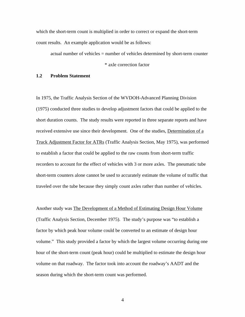
4

which the short-term count is multiplied in order to correct or expand the short-term

count results. An example application would be as follows:

actual number of vehicles = number of vehicles determined by short-term counter

* axle correction factor

1.2 Problem Statement

In 1975, the Traffic Analysis Section of the WVDOH-Advanced Planning Division

(1975) conducted three studies to develop adjustment factors that could be applied to the

short duration counts. The study results were reported in three separate reports and have

received extensive use since their development. One of the studies, Determination of a

Truck Adjustment Factor for ATRs (Traffic Analysis Section, May 1975), was performed

to establish a factor that could be applied to the raw counts from short-term traffic

recorders to account for the effect of vehicles with 3 or more axles. The pneumatic tube

short-term counters alone cannot be used to accurately estimate the volume of traffic that

traveled over the tube because they simply count axles rather than number of vehicles.

Another study was The Development of a Method of Estimating Design Hour Volume

(Traffic Analysis Section, December 1975). The study’s purpose was “to establish a

factor by which peak hour volume could be converted to an estimate of design hour

volume.” This study provided a factor by which the largest volume occurring during one

hour of the short-term count (peak hour) could be multiplied to estimate the design hour

volume on that roadway. The factor took into account the roadway’s AADT and the

season during which the short-term count was performed.

5

The other study, The Relationship of the Percentage of Trucks in the Average Daily

Traffic (ADT) to the Percentage of Trucks in the Peak Hour Volume (PHV) (Traffic

Analysis Section, February 1975), was performed because through observation, they

expected that the percentage of trucks in the AADT was normally greater than the

percentage of trucks in the peak hour volume. It was generally understood that the

temporal distribution of the percentage of trucks was not necessarily uniform over a 24-

hour period, and that truck flow did not necessarily peak during the general vehicle peak.

These elements combine to make the percentage of trucks in the peak hour less than the

overall percentage of trucks in daily traffic. However, traffic-counting techniques that

utilize manual classification are typically performed for durations shorter than 24-hours.

As a result, the WVDOT used vehicle count and classification data that were collected

manually to develop factors that relate the percentage of trucks in the peak hour to the

percentage of trucks in the AADT.

These studies are now over 25 years old. It is likely that changing travel patterns such as

increased vehicle miles traveled or changing demographics such as more vehicles per

household and an increase in the percentage of working females in West Virginia have

reduced the validity of the results of these studies for use in the traffic analyses of the

present day and the planning horizon. Also, the travel patterns of large trucks have

changed greatly over the past 25 years. In the past, goods were stored in warehouses

throughout the country and trucks were used to deliver goods to and from these

warehouses. Today, goods are delivered from the factory to the customer in a just-in-

time fashion. This has changed the operational pattern of trucks. They can no longer

6

travel predominately at night to avoid heavy traffic during the day. Another factor

related to truck operations has been the completion of the Interstate Highway System in

West Virginia. In 1975, the system was incomplete in West Virginia with many missing

links that were not attractive as through routes for commercial vehicles.

These studies had a common thread in that they were performed primarily using traffic

count data from permanent count stations in West Virginia. Currently, traffic counts are

continuously collected at permanent recorder stations; therefore, these studies can

essentially be repeated with a present day database. It would be desirable to determine

the above-mentioned parameters using current traffic count data from West Virginia

permanent counter stations.

There are additional parameters, which can be obtained from the permanent traffic

recorder data that would be of interest to WVDOT planners. One of these is the

determination of factors that relate the percentage of trucks in the average daily traffic to

the percentage of trucks in the hours currently used by the WVDOT in conducting

manual classification counts. This factor will expand the percentage of trucks counted

during a manual classification count so that a more accurate estimation of the percentage

of trucks traveling on the roadway during an entire day can be derived. This factor is

needed for pavement design, capacity analysis, and may be used to compare potential

roadway projects. The design of pavements depends both on the loads the pavement will

be exposed to, and the number of repetitions of the loads. Capacity analysis uses both the

overall traffic volume and the percent trucks in the overall volume to determine, among

7

other things, the number of lanes needed to provide a desired level of service. Project

selection may depend on the overall traffic volume and the percent trucks traveling on the

roadway. For these reasons the highway designer needs to know the percentage of trucks

in the ADT.

1.3 Project Objectives

The objectives of this study were to:

1) Establish correction factors that can be applied to the raw data from axle-

counting single pneumatic tube traffic count stations to adjust for the effect of

trucks with three or more axles on the volume counts.

2) Establish factors that use the peak hour volume to estimate the design hour

volume.

3) Establish factors that relate the percentage of trucks in the ADT to a) the

percentage of trucks in the peak hour and b) the percentage of trucks in the

hours used by the WVDOT in conducting manual classification counts.

1.4 Organization of Report

Chapter 1 has presented background to the problem and identified the problem

and study objectives. Chapter 2 contains a summary of the literature reviewed to

identify relevant information concerning the factors to be developed and the

methods used. The literature review is followed by the methodology which is

presented in Chapter 3. Project results are presented in Chapter 4. Conclusions,

recommendations, and suggestions for implementation are discussed in Chapter 5.

8

Chapter 2 LITERATURE REVIEW

2.1 Introduction

This chapter documents the literature reviewed relative to the factors developed for traffic

and truck variation from data collected through the use of permanent traffic recorders and

relates it to the current West Virginia Department of Transportation program. The scope

of this literature review was limited to examination of the Federal Highway

Administration’s (2001) Traffic Monitoring Guide and AASHTO’s Guidelines for Traffic

Data Programs (1992) since these serve as guidelines for states’ traffic monitoring

programs. The examination also included determining how two other states were

following the recommendations set forth by FHWA and AASHTO. The previously

mentioned factors studies performed by West Virginia Department of Highways in 1975

were reviewed to determine the procedures followed.

Techniques for collecting and analyzing traffic data are well established across the United

States. The FHWA Traffic Monitoring Guide (2001), and the AASHTO Guidelines for

Traffic Data Programs (1992) provide a good, up-to-date coverage of the topic and are

used as guides by all states when performing traffic counts and interpreting the output

data from these counts. The procedure guidelines from these documents are summarized

here. This is followed by discussion of the procedures and methodologies relative to the

specific data and factors of interest in this research. In addition, the three previous

studies performed in 1975 by the West Virginia Department of Highways will be

9

discussed. Pennsylvania DOT (Bureau of Planning and Research, 1999) and Michigan

(Bureau of Transportation Planning, 2000) procedures were reviewed to analyze the

procedures used by these two states to determine if they were consistent with the TMG

and AASHTO guidelines.

2.2 Traffic Monitoring Programs

2.2a Procedure Guidelines

The Traffic Monitoring Guide 2001 (Federal Highway Administration, 2001) offers

suggestions and standards to help improve and advance current programs with a view

towards the future of traffic monitoring. In addition to including a basic structure for

traffic monitoring, the TMG provides examples of how statewide data collection

programs should be structured. It also describes the analytical logic behind that structure,

and provides the information highway agencies need to maximize the efficiency of their

traffic-monitoring program.

The American Association of State Highway and Transportation Officials (AASHTO)

developed its Guidelines (AASHTO, 1992) because a general method of collecting and

evaluating traffic data was needed. A common thread linking all states programs was

needed because every state varies in their funding, staffing, and automating of traffic data

programs. The following statement from the Guidelines itself, describes other concerns

that the publication addresses:

10

“The AASHTO Guidelines specifically addresses concerns of state transportation

agencies. Also, they may be adopted for use by other governmental agencies and

private firms. If state funds are used to support the traffic monitoring work of other

agencies or firms, it is recommended that the Guidelines be followed to help ensure

comparable traffic statistics.”

The AASHTO Guidelines and the Traffic Monitoring Guide are very similar in their

approach and recommendations relating to traffic monitoring programs. The differences

between the two are as follows:

• The TMG contains the requirements set forth by the federal government which

the states are required to follow in order to receive federal-aid funds.

• The AASHTO Guidelines supplements the FHWA Traffic Monitoring Guide and

aids in the operational implementation of a state traffic data program.

2.2b Permanent and Short-Term Counts

The basic traffic-monitoring program of a state consists of short duration counts gathered

by portable recorders and continuous counts collected by permanent recorders at a

relatively small number of representative locations. The traffic on most roadways within

a state is monitored at some point every 3 years or 6 years, depending on the roadway,

but it would not be cost-effective to install a permanent counter on every roadway. The

TMG (FHWA, 2001) recommended procedure for implementing a traffic-monitoring

program includes the following steps:

11

1) Determine the statewide needs for the traffic-monitoring program.

2) Determine what continuous collection data are needed for specific projects and

what continuous collection exists or is planned for operational purposes.

3) Determine the available funding.

4) Prioritize the specific project locations.

5) Place counters at the specific project locations for which funding exists.

6) Determine how those data collection efforts can help meet statewide needs.

7) Determine additional number of additional continuous count locations needed

to meet statewide needs.

8) Prioritize these remaining statewide needs locations.

9) Allocate counters to these statewide needs locations on the basis of their

priority and the available funding.

10) If funding remains after statewide needs have been met, place additional

continuous counters at the specific project sites for which counters are

currently not allocated.

The Traffic Monitoring Guide (FHWA, 2001) and the AASHTO Guidelines (1992) both

discuss the development of an axle correction factor, but the other factors developed in

this study are not mentioned. The documents mention that traffic volume, vehicle

classification, and truck weight data are all part of a traffic-monitoring program, but the

other factors developed in this study are not discussed.

12

The short duration counts are usually collected for 48-hours at a large number of

locations within the state to provide coverage. Permanent counters are installed at

representative locations throughout the state to provide time-of-day, day-of-week, and

seasonal travel patterns, all of which allow the development of factors needed to correct

or expand the short-term count data into accurate estimates of annual traffic conditions.

An example of data correction would be a factor developed by using information

provided by a group of permanent count stations that could be applied to short-term

pneumatic tube traffic counts to correct for the effect of three or more axle trucks on the

volume counts. An example of a factor developed to expand on a short-term count would

be a PHV to DHV factor that would allow an agency to perform a 48 hour count,

determine the PHV which occurred during that 48 hours, and applying the factor to

determine the DHV on the roadway.

2.2c Error-Checking Methodologies

According to the Traffic Monitoring Guide (FHWA, 2001), two types of error are

possible in collecting and analyzing traffic data. The two types of error are 1) errors in

collection, and 2) errors in editing. A wide range of factors including power failure,

recorder malfunction, and detector malfunction are sources of invalid data and missing

data from the permanent counters. The errors resulting from these malfunctions include

missing days and/or missing hours of data, negative numbers included in the figures, and

vehicle classification errors. How these errors are handled can have a major impact in the

13

validity of the factors generated. Depending on the handling of these errors, errors in the

editing process can result.

Both documents stated that, in terms of short-term counts, the minimum data requirement

is a duration of 48 hours. If there is found to be a problem in the data such as missing

data due to equipment malfunction, it is recommended by AASHTO (1992) and the

Traffic Monitoring Guide (FHWA, 2001) that the count be redone. When permanent

counts are visually found to contain errors, there is not a correction process. The only

manual step in editing permanent counter data is to review the data set for completeness

and to exclude data that has been rendered invalid through a power failure or machine

malfunction. The following statements from AASHTO (1992) address the issue of

attempting to manually correct erroneous data:

“Some current traffic editing programs estimate missing or edit-rejected data.

This practice, termed “imputation”, is not recommended.”

“Subjective editing procedures for identifying and imputing missing or invalid

data are discouraged, since the efforts of such data adjustments are unknown and

frequently bias the resulting estimates.”

The AASHTO Guidelines (AASHTO, 2001) state that there should be a sufficient

number of days of valid traffic measurements during a year to compute average traffic

characteristics at the site. The number of days needed is determined by whether or not an

14

automated editing process is used to evaluate the recorded data. If automated edits are

performed, it is recommended that agencies adopt a one-day minimum of edit-accepted

data for each day of the week and each month of the year. Until agencies have

implemented automated edits, it is recommended by AASHTO that a two-day minimum

for each day of the week, each month of the year, be adopted. These statements from

AASHTO and supported by the TMG are to be strictly followed so that the procedure

used to determine the necessary factors is valid and complies with the AASHTO-

recommended procedure.

2.3 Developing Axle Correction Factors Using Vehicle Classification Counts

2.3 a Overview

According to the Traffic Monitoring Guide (FHWA, 2001), in the 1980’s, the Federal

Highway Administration (FHWA) developed a vehicle classification system containing

thirteen (13) categories of vehicles. According to the TMG (FHWA, 2001), all states

currently use this classification system or a similar variation. Permanent counters

recognize the different vehicle classifications and record the number of vehicles in each

category that traveled over the counter during the designated time period. Reporting of

the data in fifteen-minute and one-hour time intervals are common. Axle corrections

factors can be developed from these data to adjust axle counts to an accurate estimate of

the actual number of vehicles which traveled over the tube counter.

15

Permanent traffic recorders use two in-pavement inductive loops to record axle spacing

and vehicle classification, as well as speed, date, and time. Portable devices using a

single pneumatic tube axle sensor can only count the number of axles that travel over

them. The data from the permanent counters are retrieved and processed, and factors

are developed and used to correct the data collected from the short-term pneumatic tube

axle counters.

2.3b Determination of Axle Adjustment Factors

An axle correction factor must be derived from the information provided by the

permanent counters and applied to the short-term single pneumatic tube counter so its

information can have validity and be useful to traffic engineers. The following statement,

from the Traffic Monitoring Guide (FHWA, 2001), states the importance of performing

an axle correction count to adjust permanent traffic volume counts using the chart of

values included in the TMG manual.

“Where classification counts exist (particularly those that use the 13 FHWA

classes), a much more accurate axle correction factor can be computed by

assigning an average number of axles per vehicle for each vehicle on that road.”

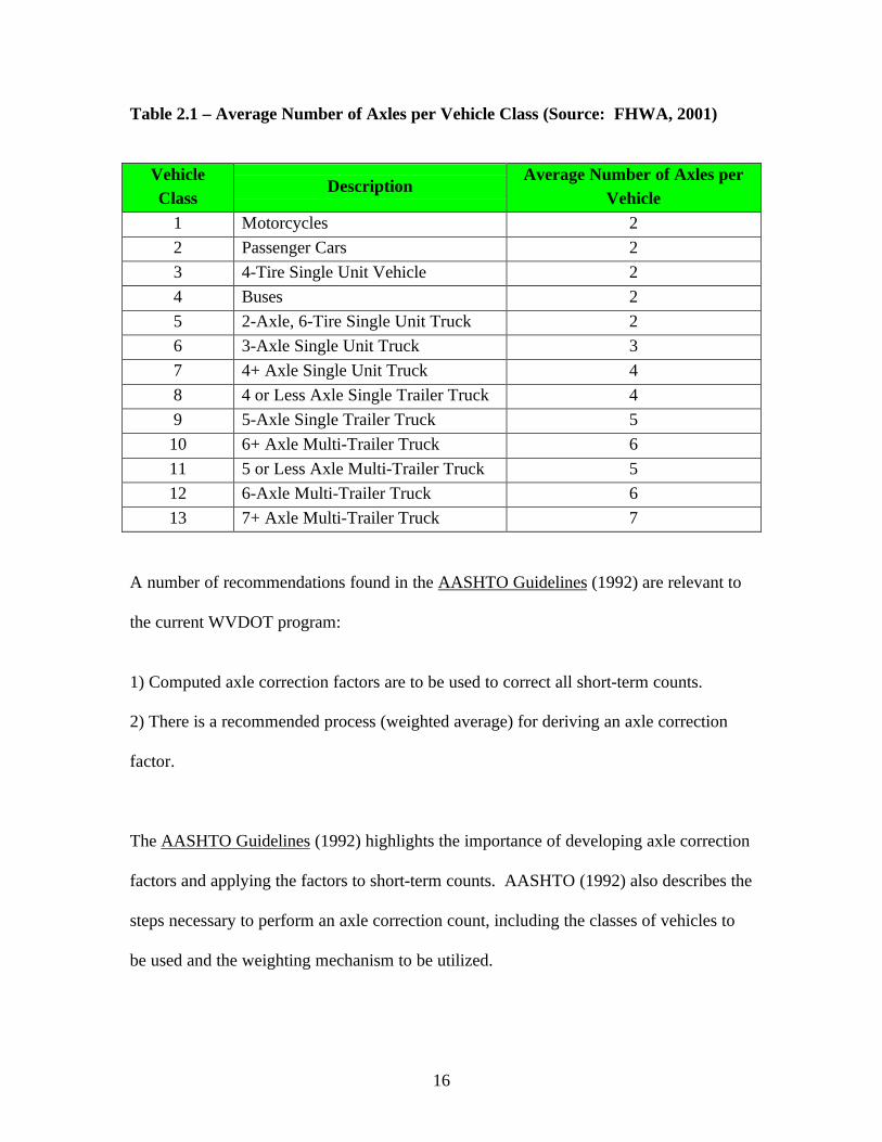
The conversion chart, found in the Traffic Monitoring Guide (FWHA, 2001), included as

Table 2.1, lists the suggested values to be used for each vehicle class when calculating an

axle adjustment factor.

16

Table 2.1 – Average Number of Axles per Vehicle Class (Source: FHWA, 2001)

VehicleClass

DescriptionAverage Number of Axles per

Vehicle1 Motorcycles 22 Passenger Cars 23 4-Tire Single Unit Vehicle 24 Buses 25 2-Axle, 6-Tire Single Unit Truck 26 3-Axle Single Unit Truck 37 4+ Axle Single Unit Truck 48 4 or Less Axle Single Trailer Truck 49 5-Axle Single Trailer Truck 510 6+ Axle Multi-Trailer Truck 611 5 or Less Axle Multi-Trailer Truck 512 6-Axle Multi-Trailer Truck 613 7+ Axle Multi-Trailer Truck 7

A number of recommendations found in the AASHTO Guidelines (1992) are relevant to

the current WVDOT program:

1) Computed axle correction factors are to be used to correct all short-term counts.

2) There is a recommended process (weighted average) for deriving an axle correction

factor.

The AASHTO Guidelines (1992) highlights the importance of developing axle correction

factors and applying the factors to short-term counts. AASHTO (1992) also describes the

steps necessary to perform an axle correction count, including the classes of vehicles to

be used and the weighting mechanism to be utilized.

17

“At each vehicle classification count site, the number of vehicles is totaled by

each of the 13 FHWA vehicle classifications. The number of the vehicles in each

classification is multiplied by the number of axles in the classification. These are

summed, and divided by the total number of vehicles. This is the average number

of axles per vehicle at the permanent counter site. This figure is summed for all

similarly grouped count sites, and divided by the number of counters. The result

is the group mean axles per vehicle.”

2.3c Grouping the Data Collection Sites

Once information is gathered from all of the permanent traffic recorders throughout the

state, sites are grouped so that they are statistically similar based on several factors.

These factors include geography, roadway classification, recreational usage, and any

other relevant variable that would allow the sites to by grouped in a statistically

significant manner. The Traffic Monitoring Guide (FHWA, 2001) recognizes the

difficulty involved with grouping sites, as can be seen by the following statement:

“The grouping process is made more difficult and error prone because the

appropriate definition of a “group” changes depending on the characteristics being

measured.”

Grouping roadways once the factors are calculated from the permanent traffic counters is

essential; for the short term counts will not all be taken from the same roadways from

18

which the permanent counters were used. For this reason, groups of similar roadways

need to be formed so that a short-term count can be related to a factor that relates to that

particular type of roadway. The TMG (FHWA, 2001) recommends the groups shown in

Table 2.2 as a minimum.

Table 2.2 –Roadway Groups Recommended by Traffic Monitoring Guide

(FHWA, 2001)

Recommended Group HPMS Functional Code

Interstate Rural 1

Other Rural 2,6,7,8

Interstate Urban 11

Other Urban 12,14,16,17

Recreational Any

Testing the quality of the selected groups is a key aspect to any grouping procedure. The

following statement from the TMG (FWHA, 2001) includes their recommended methods

of testing the quality of the groups.

“The quality of a given factor group can be examined in two ways. The first is to

graphically examine the traffic pattern present at each site in the group. Graphs

give an excellent visual description of whether different data collection sites have

similar travel patterns. The second method is to compute the mean and standard

deviation for various factors that the factor group is designed to provide. If these

factors have small amounts of deviation, the roads can be considered to have

19

similar characteristics. If the standard deviations are large, the road groupings

may need to be revised.”

A number of observations found in the AASHTO Guidelines (1992) are relevant to the

current WVDOT program. West Virginia, as previously mentioned, currently has 52

permanent traffic recorder stations located throughout the state on various classes of

roadways. The data from these locations must be grouped together in a statistically

sound manner to ensure the validity of the factors. Grouping the data collected involves

two steps: The first step is to group the sites so that the most similar sites are in the same

group. The second is to associate short-term count stations to the long-term permanent

count groups. The AASHTO Guidelines (1992) recommend that when grouping the

permanent count locations, the variability between permanent count locations within the

same group should be minimized, while the variability found between groups of

permanent count locations should be maximized. AASHTO (1992) also states that when

forming the permanent counter locations into groups, the recommended rule-of-thumb is

that there should be a minimum of five counters in each of the defined groups. Once the

permanent count locations have been grouped in a statistically verified manner, the

locations of short-term traffic counts must be associated with the defined groups of

permanent count locations. If data fail to group according to functional classification,

AASHTO (1992) recommends using a method of combining the functional classification

of the roadway with the geographic location of the count site within the state to obtain a

more effective grouping.

20

2.3d Variation of Factors with Time

Two facets of time are relevant when discussing the variation of the factors derived in

this study. First and foremost, 25 years has passed since the WVDOH last developed the

factors relevant to this study. The passing of 25 years necessitates the need for the

development of a new set of factors to be used in the design and analysis of the roadways

of West Virginia. Second, travel patterns of vehicles vary based on time of the day, day

of the week, and season of the year. The variance of travel patterns based on day of the

week and season of the year is the reason for the factors being analyzed based on these

time-related factors.

As mentioned in Chapter 1, in 1975, three studies were performed by the West Virginia

Department of Highways to determine the following factors:

1) A truck adjustment factor for short-term counters

2) Estimating DHV by using the PHV

3) Estimating the % Trucks in the ADT by using the % Trucks in the PHV

In performing the truck adjustment factor study (Traffic Analysis Section, May 1975), 62

temporary stations were established for the purpose of the study, at which a short-term (8

to 24 hour) manual count and a longer count lasting from 24 hours to 7 days was

performed. The percentage of trucks and traffic volume was used to classify the roadway

as either an expressway/trunkline or feeder/local roadway. The results from the truck

adjustment factor study were as follows:

21

Actual count = 0.92974 * (short-term count) for feeders and locals

Actual count = 0.88589 * (short-term count) for expressways and trunklines

In this case, as would be expected, the higher roadway classifications experience a

greater volume of truck traffic. This 1975 study documented that the magnitude of the

factor depends upon the type of highway on which the count was performed.

The data for the PHV to DHV study (Traffic Analysis Section, December 1975) was

derived from the permanent traffic recorder record for the year 1972. Analysis of

variance (ANOVA) was performed to determine if there was a significant difference in

the factors developed using the PHV, the 10th highest hourly volume and the 30th highest

hourly volume. This test determined that factors should be derived separately for the 10th

highest and 30th highest hourly volumes. The study also determined that the Annual

Average Daily Traffic (AADT) was a significant player in the factor’s development.

Separate factors were determined for roads with an AADT less than or equal to 500

vehicles, and roads with AADT greater than 500 vehicles. The equation used to derive

the factor relating PHV to DHV can be found below and the resulting factors are reported

in Table 2.3.

22

DHV = Bij * (PHV)

where Bij is the factor relating the PHV to the DHV from Table 2.3

i = 1 if AADT � 500

= 2 if AADT > 500

j = 1, 2, 3, 4; depending on the quarter the count was taken

Table 2.3 – Factors (Bij) from 1975 WVDOH Study Relating PHV to DHV

(Source: Traffic Analysis Section, December 1975)

i = 1 i = 2

j = 1 Dec - Feb 1.42257 1.3316j = 2 Mar - May 1.32577 1.23895j = 3 Jun - Aug 1.28892 1.20249j = 4 Sept - Nov 1.23583 1.15346

In the study estimating truck percentages (Traffic Analysis Section, February 1975), data

were collected from manual classification counts performed 4 times a year (one each

season) at seventeen truck weight stations. Analysis of variance found that there was a

significant difference in the factors developed for each season, thus they were reported by

season. The equation used is found below and the results found from the estimation of

the % Trucks in the ADT by using the % Trucks in the PHV are reported in Table 2.4.

Percentage of trucks in ADT = Bi * Percentage of trucks in peak hour volume

where Bi is the seasonal factor from Table 2.4

23

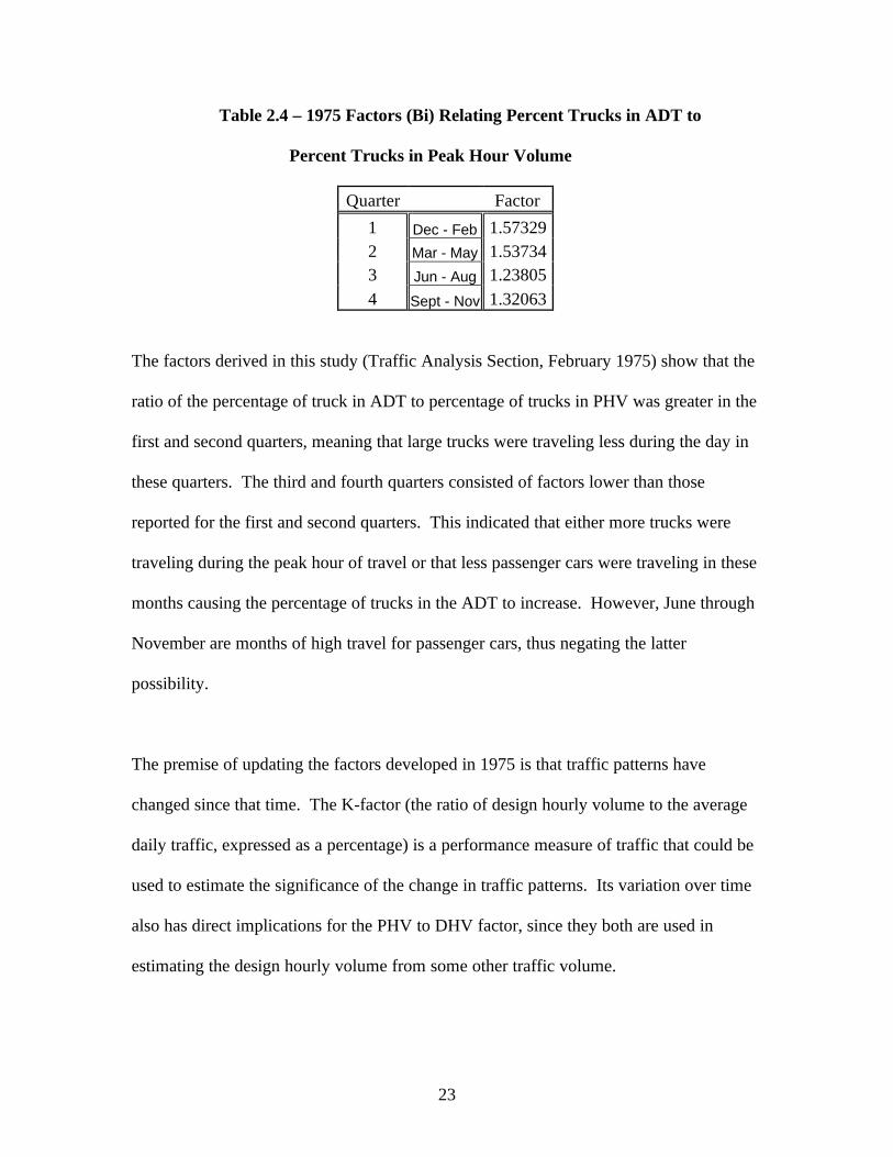
Table 2.4 – 1975 Factors (Bi) Relating Percent Trucks in ADT to

Percent Trucks in Peak Hour Volume

Quarter Factor1 Dec - Feb 1.573292 Mar - May 1.537343 Jun - Aug 1.238054 Sept - Nov 1.32063

The factors derived in this study (Traffic Analysis Section, February 1975) show that the

ratio of the percentage of truck in ADT to percentage of trucks in PHV was greater in the

first and second quarters, meaning that large trucks were traveling less during the day in

these quarters. The third and fourth quarters consisted of factors lower than those

reported for the first and second quarters. This indicated that either more trucks were

traveling during the peak hour of travel or that less passenger cars were traveling in these

months causing the percentage of trucks in the ADT to increase. However, June through

November are months of high travel for passenger cars, thus negating the latter

possibility.

The premise of updating the factors developed in 1975 is that traffic patterns have

changed since that time. The K-factor (the ratio of design hourly volume to the average

daily traffic, expressed as a percentage) is a performance measure of traffic that could be

used to estimate the significance of the change in traffic patterns. Its variation over time

also has direct implications for the PHV to DHV factor, since they both are used in

estimating the design hourly volume from some other traffic volume.

24

According to AASHTO, (2001) the K-factor, based on data obtained in a traffic count

program, is developed and applied system-wide. In other cases, factors may be

developed for different facility classes or different areas of an urban region, or both.

A study performed by in 1988 (Sharma and Oh, 1988) researched, among other things,

what affects the value of the K-factor. The conclusions drawn from their research was

that the K-factor is a function of the nature of travel (rural, urban, suburban, or

recreational) and that the K-factor remains relatively stable over time as long as the

nature of travel remains the same. K-factor values plotted for a site from 1973 through

1985 showed that K-factor values decreased slightly as AADT increased, and then rose

slightly when AADT decreased.

Another study performed in 1988 (Walters and Poe, 1988) stated how the K-factor varies

depending on the distance from a central business district (CBD) of large cities in Texas.

Their results showed that the K-factor decreased the closer to the CBD the measurement

was taken, and increased the farther away from the CBD the measurement was taken.

This was due to the fact that congestion was greatest in the CBD and that congestion

decreased as traffic dispersed from the congested area. They also stated that the K-factor

tends to decline over time as congestion on a roadway increases.

In spite of statements to the contrary in some published literature (Sharma and Oh, 1988),

there is actually very little documented research concerning how K-factors have varied

25

over time. (Walters and Poe, 1988) However, among the studies that were published, the

following was learned about the variation of K over time:

• The K-factor can vary up to 35% over the course of one year for different sections

of the same roadway.

• K values remain relatively stable over time.

• K values decrease when the facility reaches capacity during the peak hour.

Therefore, since vehicle-miles of travel and roadway congestion has continually

increased over the last several decades, it can be concluded that K-values in general

should be lower now than in 1975. It is recommended that research be performed using

actual traffic data to support this hypothesis.

2.4 Percentage of Trucks in the Traffic Stream

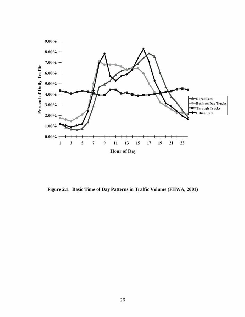
Truck volumes vary significantly by time of day and day of week as illustrated by

Figures 2.1 and 2.2. Because three of the four factors of interest to this study deal

directly with the travel patterns of large trucks, the variation of truck travel with respect

to time is important when developing these factors. Figure 2.1 shows that the hours of

peak passenger car travel differ slightly from the hours of peak truck travel. Figure 2.2

provides insight into how travel patterns vary from weekday to weekend. These figures

were used in developing an understanding of how passenger car and truck volumes vary

with hour of the day.

26

Figure 2.1: Basic Time of Day Patterns in Traffic Volume (FHWA, 2001)

27

Figure 2.2: Typical Hour of the Day Travel Patterns for Large Trucks

(FHWA, 2001)

The methodology behind calculating the percent trucks in the traffic stream can be

understood by reading the following excerpt from the Traffic Monitoring Guide (FHWA,

2001):

“Because the volumes of cars and trucks often are very different, the effect of

these different time-of-day patterns on summary statistics such as “percent trucks”

and “total volume” can be unexpected. Often, in daylight hours, car volumes are

so high in comparison to truck volumes that the car travel pattern dominates, and

28

the percentage of trucks is very low. However, at night on that same roadway, car

volumes may decrease significantly while through-truck movements continue, so

that the truck percentage increases considerably, and the total volume declines

less than the car pattern would predict. Because these changes can be so

significant, it is important to account for them in the design and execution of the

traffic monitoring program, as well as in the computation and reporting of

summary statistics.”

Estimating the percentage of trucks in the average daily traffic can be accomplished by

developing a factor which relates the percent trucks in the ADT to 1) the percent trucks in

the peak hour, or 2) the percent trucks in the manual count hours. The first factor allows

traffic engineers and roadway designers to determine the percentage of trucks using the

roadway on a daily basis based on the percentage of trucks in the traffic stream during the

peak hour. The second factor relates the percentage of trucks in the ADT to the

percentage of trucks in the manual count hours used by the WVDOT, which are: 7am-

10am, 11am-1pm, and 2pm-6pm. These hours are used by the WVDOT to ensure that

the morning, noon, and evening peak hours were counted. The West Virginia

Department of Transportation performs manual classification counts Monday through

Thursday. Because trucks do not follow the same travel pattern as passenger cars, a factor

must be applied to the percentage of trucks found during the manual classification count

hours so that an accurate estimate of the percentage of trucks can be determined from a

short-term count.

29

2.5 Relationship of Design Hour Volume and Peak Hour Volume

The design hour volume is defined by both AASHTO (1992) and FHWA (2001) as the

hourly traffic volume, usually represented by the thirtieth highest hourly volume of the

future year, chosen for design. The peak hour volume is the greatest hourly volume of

traffic counted during one day’s time. Using permanent traffic counters, the traffic

volumes for every day of the year can be calculated, sorted based on total volume, and

plotted on a graph from the highest volume experienced to lowest. The design hourly

volume is then chosen based on where the plotted curve levels out. Use of the design

hourly volume ensures that the roadway is not designed based on unreasonably high

traffic volumes that occurred during special incidents such as football games or holidays.

It is recommended by both AASHTO (1992) and FHWA (2001) that the hour chosen lies

between the 10th and 50th highest hourly volumes for the year. The factor derived based

on the permanent count stations should then be applied to temporary counts so that the

DHV of a roadway can be estimated with the peak-hour count found during a 48-hour

count. The DHV of a roadway is greater than the PHV for most days if the short-term

count day is selected so that special incidents are avoided.

2.6 Other States’ Programs

As noted earlier, both PENNDOT and the Michigan DOT documents were examined.

Both agencies published findings from their traffic monitoring programs. It was

apparent that PENNDOT (Bureau of Planning and Research, 1989) and Michigan DOT

30

(Bureau of Transportation Planning, 2000) both used the TMG and AASHTO

recommended process of developing axle correction factors. Both began with raw count

data collected at permanent count stations located throughout the state. These count

stations were then grouped into statistically similar groups based on functional class or

geography. The factors developed from the permanent count stations were then applied

to short-term counts performed with axle counters such as pneumatic tubes.

The traffic pattern groupings (TPG) used by PENNDOT and the axle correction factors

are shown in Table 2.5. Functional classification, geography, and urban/rural

characteristics were used to group the locations.

Table 2.5 – PENNDOT’S Traffic Pattern Groupings

TPG 1 Urban InterstateTPG 2 Rural InterstateTPG 3 Urban Other Principal ArterialsTPG 4 Rural Other Principal ArterialsTPG 5 Urban Minor Arterials, Collectors, Local RoadsTPG 6 North Rural Minor ArterialsTPG 7 Central Rural Minor ArterialsTPG 8 North Rural Collectors and Local RoadsTPG 9 Central Rural Collectors and Local RoadsTPG 10 Special Recreational

The axle correction factors developed in the PENNDOT study will be used to draw a

comparison with the current WVDOH study. The factors reported by PENNDOT for the

ten traffic pattern groups are shown in Table 2.6.

31

Table 2.6 – Axle Correction Factors Reported by PENNDOT

TPG Correction Factor1 0.8402 0.7023 0.9414 0.8975 0.9806 0.9357 0.9508 0.9669 0.9710 0.968

The Michigan DOT document was their procedures manual. The manual did not report

any specific factors, but provided a list of the traffic pattern groups used when developing

factors. The traffic pattern groups were derived based not on functional classification;

rather they were grouped based on urban/rural characteristics, geography, and

recreational uses. The groupings used by Michigan DOT are shown in Table 2.7.

Table 2.7 – Michigan DOT’s Traffic Pattern Groupings

Pattern Description

1 Urban/Rural2 Rural3 Urban4 Recreational5 Straits Area Recreational6 Rural/Recreational7 Urban Area Limit

32

2.7 Concluding Remarks

In summary, both the Traffic Monitoring Guide (FHWA, 2001) and the AASHTO

Guidelines for Traffic Data Programs (1992) emphasize the need for an axle adjustment

factor. Once the data are collected for the thirteen FHWA vehicle classifications, both

documents recommended grouping the sites by similar characteristics such as functional

class, geography within the state, urban/rural characteristics, and seasonality

(recreational). Testing how well the permanent traffic counters fit into the grouped

categories can be performed by using graphical analysis or cluster analysis. Once the

groups are finalized, each traffic counter in the state can then be placed into one of the

groups. This will give each counter a factor for every day of the year that will convert

the axle count into a more useful traffic count based on the time-of-day, day-of-week, and

seasonal travel pattern.

In 1975, the WVDOH developed axle correction factors, factors for estimating DHV by

using the PHV, and factors used for estimating the % Trucks in the ADT by using the %

Trucks in the PHV. These factors are over 25 years old. Since their development, the

demographics of the state, travel patterns, and commercial vehicle operations have

changed. Thus, these factors need to be updated to provide the West Virginia Division of

Highways with valid current factors.

33

Chapter 3 METHODOLOGY

3.1 Data Acquisition

The data for this project was provided by the Traffic Analysis Section of Planning and

Research Division of the West Virginia Department of Transportation for the 52

permanent count stations located throughout the state. The raw data was from counts

performed for the years 1995 and 1996, the most recent data the WVDOT had gathered

from the permanent count stations. Traffic volumes and classification data were recorded

every hour of the year for every lane at every station. Vehicles were classified into one

of the thirteen FHWA vehicle classification categories. Functional classes considered

were consistent with the Traffic Monitoring Guide (FHWA, 2001). The number of sites

in each functional class as well as the descriptions of each functional class are shown in

Table 3.1.

Table 3.1 – Number of Sites in Each Functional Class

Functional Functional Class Number of Sites Number of SitesClassification Description 1995 1996

1 Rural interstate 7 72 Rural principal arterial – other 4 46 Rural minor arterial 10 87 Rural major collector 11 1111 Urban interstate 5 512 Urban principal arterial – other freeways 2 214 Urban other principal arterial 5 516 Urban minor arterial 3 317 Urban collector 1 1

Total Sites 48 46

34

Note that the numbers vary from 1995 to 1996 and add up to less than 52 count stations

because some sites were not included in the raw data and others had many data errors

and, therefore, had to be discarded. Of the 104 total count stations (52*2=104) used

between both 1995 and 1996, 9 sites were missing all of their data. These sites included

four from functional class 1, one from functional class 2, two came from functional class

6, and two were missing from functional class 11.

The raw data files consisted of one file for every day of the year. The files from each site

for a given year needed to be collapsed into one large file. The program “Reporter” was

provided by the WVDOT and was used to perform the conversion of the data files from

their collected format into a Microsoft Excel format. Once “Reporter” was implemented,

the 365 Excel files had to be organized into one large file so that further analysis could

take place. The following workbooks were created for each site in an effort to further

organize the data: “by lane”, “by direction”, “by hour”, “by day”, and “by month.”

The next step was to determine and identify the types of errors contained in the raw data

files and eliminate the errors so the results would be accurate. The errors were detected

primarily manually at the database organization stage, but also when the factors were

computed (because they had a significant impact of the factors). Types of errors

identified included the following: 1) missing data, 2) unreasonably large numbers, 3)

functional classes switched (functional classes 1 and 2), and 4) zeros. Errors ranged from

81% of the days containing errors to 4% of the days in error. Overall, the data for 1996,

averaging 28% of the days containing errors per site, contained more erroneous data than

35

1995 which averaged 25% of the days in error per site. These figures are skewed slightly

because several sites were completely removed from 1996 because they contained so

many errors, or no data at all, thus they were not included in the raw data sent by the

WVDOT. By recommendation of the AASHTO Guidelines for Traffic Data Programs

(1992) and the Traffic Monitoring Guide (FHWA, 2001), data in error were omitted from

further analysis, and no data containing errors was corrected and used in the formulation

of any factors. The data was then analyzed in accordance with the Traffic Monitoring

Guide (FHWA, 2001) and the AASHTO Guidelines (1992).

The factors of interest were:

1) An axle correction factor that could be applied to short-term single pneumatic tube

axle counts to counteract the effect of 3 or more axle trucks on vehicle counts.

2) A method of estimating the design hour volume by developing a peak hour volume to

design hour volume factor.

3) Determine a factor relating the Percent Trucks in the ADT to Percent Trucks in the

Peak Hour.

4) Determine a factor relating the Percent Trucks in the ADT to Percent Trucks in the

Manual Count hours.

The factors were developed using the 1995 data, and then again using the data from 1996.

By request of the WVDOT, the factors developed using the 1996 database were used to

validate the procedure used to determine the 1995 factors. Previously overlooked errors

36

were discovered when the 19965 and 1996 factors were plotted and compared. These

errors were located and removed.

3.2 Axle Correction Factor Procedure

The process of developing the axle correction factors began by assigning the 13 FHWA

vehicle classes a number of axles as recommended by the TMG (FHWA, 2001) and

previously shown in Table 2.1. The actual number of vehicles was known by tabulating

the vehicles in the thirteen vehicle classifications counted by the permanent count station.

The number of vehicles that would have been reported by the pneumatic tube counter

would be the total number of axles divided by two. The following equation demonstrates

how the factor was developed. The actual number of vehicles that traveled over the

pneumatic tube count station can be determined by multiplying the number of vehicles

determined by the short-term pneumatic tube counter by the axle correction factor.

Axle correction factor = actual number of vehicles . # of vehicles reported by pneumatic tube counter

where:

# of vehicles reported by pneumatic tube counter = total # of axles 2

It should be noted that the raw data file provided by the WVDOH included 15 vehicle

classifications. This fact was brought to the attention of the WVDOH project monitor.

The response was that classifications 1 through 13 are the FWHA classes, and 14 and 15

are columns in which vehicle are categorized when the traffic counter did not categorize

37

the vehicle. These columns were simply disregarded and not included in the factor

development.

The average numbers of axles per vehicle class were then applied to the “by day”

summaries. Columns calculated included number of axles, short-term raw count, real

count, and real / raw. The real divided by raw is the axle correction factor for that day.

The axle correction factors were then developed for the day of the year regardless of

month, by month, and by quarter.

The next step was to establish a method of grouping the factors for the 52 sites in a

statistically significant manner. The TMG (FHWA, 2001) states that rural interstates and

urban interstates, functional classes 1 and 11, respectively, should both stand alone as

groupings. Grouping, according to the TMG, should then be made based on functional

classification, geography, or other characteristics that would allow the sites to be grouped

in a statistically significant manner. Grouping by functional class, which included the

aggregation of different functional classes in a few was the method utilized in this

project.

As in the 1975 study, single-factor analysis of variance, (ANOVA) was also used to

perform the statistical analysis throughout the project. Single-factor ANOVA involves

the analysis either of data sampled from more than two numerical populations or data

from an experiment in which more than two treatments have been used. Single-factor

ANOVA focuses on a comparison of more than two populations. In the case of this

project, the means were compared by day of the week, by month, and by quarter.

38

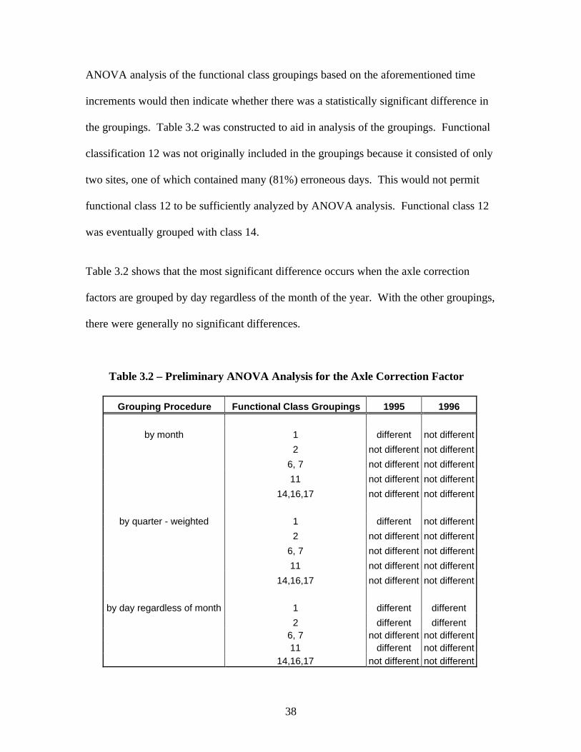
ANOVA analysis of the functional class groupings based on the aforementioned time

increments would then indicate whether there was a statistically significant difference in

the groupings. Table 3.2 was constructed to aid in analysis of the groupings. Functional

classification 12 was not originally included in the groupings because it consisted of only

two sites, one of which contained many (81%) erroneous days. This would not permit

functional class 12 to be sufficiently analyzed by ANOVA analysis. Functional class 12

was eventually grouped with class 14.

Table 3.2 shows that the most significant difference occurs when the axle correction

factors are grouped by day regardless of the month of the year. With the other groupings,

there were generally no significant differences.

Table 3.2 – Preliminary ANOVA Analysis for the Axle Correction Factor

Grouping Procedure Functional Class Groupings 1995 1996

by month 1 different not different

2 not different not different 6, 7 not different not different 11 not different not different 14,16,17 not different not different

by quarter - weighted 1 different not different 2 not different not different 6, 7 not different not different 11 not different not different 14,16,17 not different not different

by day regardless of month 1 different different 2 different different

6, 7 not different not different 11 different not different 14,16,17 not different not different

39

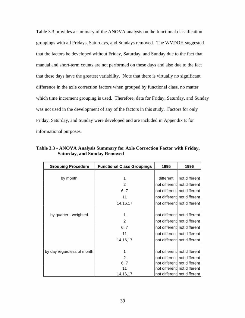
Table 3.3 provides a summary of the ANOVA analysis on the functional classification

groupings with all Fridays, Saturdays, and Sundays removed. The WVDOH suggested

that the factors be developed without Friday, Saturday, and Sunday due to the fact that

manual and short-term counts are not performed on these days and also due to the fact

that these days have the greatest variability. Note that there is virtually no significant

difference in the axle correction factors when grouped by functional class, no matter

which time increment grouping is used. Therefore, data for Friday, Saturday, and Sunday

was not used in the development of any of the factors in this study. Factors for only

Friday, Saturday, and Sunday were developed and are included in Appendix E for

informational purposes.

Table 3.3 - ANOVA Analysis Summary for Axle Correction Factor with Friday,Saturday, and Sunday Removed


by month 1 different not different

2 not different not different 6, 7 not different not different 11 not different not different 14,16,17 not different not different

by quarter - weighted 1 not different not different 2 not different not different 6, 7 not different not different 11 not different not different 14,16,17 not different not different

by day regardless of month 1 not different not different 2 not different not different 6, 7 not different not different 11 not different not different 14,16,17 not different not different

40

The decision was then made to re-evaluate some of the functional class groupings to

ensure that they were grouped in the best possible manner. The functional class

groupings analyzed were as follows:

2, 6, and 712 and 1416 and 1712, 14, 16, and 17

After analyzing the factors developed by such groupings, it was decided that the

functional class groupings should be as follows:

Group 1) 1 Rural interstateGroup 2) 2 Rural principal arterial – otherGroup 3) 6 and 7 Rural minor arterial, Rural major collectorGroup 4) 11 Urban interstateGroup 5) 12 and 14 Urban principal arterial – other freeways,

Urban other principal arterialGroup 6) 16 and 17 Urban minor arterial, Urban collector

Factors were developed for these new groupings (still excluding Friday, Saturday, and

Sunday) for the day of the week, by month, and by quarter. ANOVA analysis could not

be performed on the new groupings, since some groups included only three sites.

ANOVA was performed on the sites when they were a part of larger groupings.

3.3 Estimating Design Hour Volume

The following equation was used in determining the peak hour to design hour factor:

Design Hour Factor = Design Hour Volume Peak Hour Volume

41

In order to correctly choose the DHV for each site, graphs of the 100-300 highest hourly

volumes were made for each site.

The DHV was chosen visually, based on where the curve leveled. Figure 3.1 presents an

example of how the DHV volumes were chosen. The 30th highest hourly volume usually

falls around this region, thus it is used as a standard approach. But because of the

missing data, rather than choosing the 30th highest hourly volume, the DHV was chosen

based on where the curve leveled out. At this point, the chosen volume would represent

the majority of the highest volume hours in the year, but not include the extraordinarily

high hourly volumes such as would be attributable to special events.

42

The design hourly volume for each site was then divided by the peak hour volume for

each day, creating the factor. The factors were then combined by day regardless of

month, by month, and by quarter. The same functional class groupings identified with

the axle correction factors were used. ANOVA analysis was then performed on the

functional classification groupings to ensure that the same groupings would be sufficient.

Table 3.4 was constructed to aid in the evaluation of the groupings. Table 3.4 shows that

all grouping procedures yielded statistically significantly different values. This led to the

conclusion that the day of the week by month should be used to report the factors.

Table 3.4 - Preliminary ANOVA Analysis for the PHV to DHV Factor


by month 1 different not different 2 not different different 6, 7 different different 11 not different not different 14,16,17 different not different

by quarter - weighted 1 different not different 2 not different different 6, 7 different not different 11 not different not different 14,16,17 not different not different

by day regardless of month 1 different not different 2 not different different

6, 7 different not different 11 not different not different

14,16,17 different not different

43

For the reasons previously cited, the groupings were re-evaluated with Friday, Saturday,

and Sunday removed from the database. Table 3.5 shows the results of the ANOVA

analysis performed.

Table 3.5 - ANOVA Analysis Summary for PHV to DHV Factor with Friday,Saturday, and Sunday Removed


by month 1 not different not different 2 not different not different

6, 7 not different not different 11 not different not different 14,16,17 not different not different

by quarter - weighted 1 not different not different 2 not different not different 6, 7 not different not different 11 not different not different 14,16,17 not different not different

by day regardless of month 1 not different not different 2 not different not different 6, 7 not different not different

11 not different not different

14,16,17 not different not different

The decision was then made to re-evaluate the functional class groupings to ensure that

they were grouped in the best possible way. The same conclusion was reached as before

in the axle correction factor. The functional class groupings were as follows:

Group 1) 1 Rural interstateGroup 2) 2 Rural principal arterial – otherGroup 3) 6 and 7 Rural minor arterial, Rural major collectorGroup 4) 11 Urban interstateGroup 5) 12 and 14 Urban principal arterial – other freeways,

Urban other principal arterialGroup 6) 16 and 17 Urban minor arterial, Urban collector

44

Because high AADT facilities may have more uniform peaking characteristics due to

capacity constraints, AADT was used to further stratify the sites. The AADT was

determined by averaging the daily volumes for an entire year. A yearly factor was

calculated for each site by taking the average of the day of the month factors. This led to

48 factors being averaged together (4 days in the week multiplied by 12 months of the

year). The functional classification groupings were then sorted based on their AADT and

the factors were analyzed. Table 3.6 shows the relationship between the AADT and the

PHV to DHV factor. The results of this analysis were that 1) a breakpoint in functional

class 1 occurred at 30,000 vehicles in the AADT, thus two different factors would be

developed for this group, and 2) a breakpoint occurred in the grouping of functional

classifications 6 and 7 around 5,000 vehicles in the AADT. Separate factors would be

developed for this grouping based on this AADT relationship.

Due to the reporting of the factors in such an expanded manner, the missing and flawed

data caused by machine malfunctions created difficulties in performing an ANOVA

analysis on the data. This caused many statistical problems. For example, a functional

class that contains eight sites may only have two sites that contain a value for Tuesday in

November.

3.4 Relationship of % Trucks in the ADT to % Trucks in the Peak Hours

At each station for each day, the peak hour was selected and the percentage of trucks was

determined. The percentage of trucks for the entire day was also determined. The factor

was calculated as follows:

factor = % trucks in ADT % trucks in PHV

Functional Site Percent AADT PHV to DHV Class in Err Factor

1 50 43% 45500 1.201 39 20% 34500 1.381 3 38% 29000 1.871 47 28% 23500 1.861 5 9% 18000 1.671 53 10% 16000 1.991 1 5% 11500 2.00

2 11 44% 12300 1.302 9 28% 11400 1.272 10 8% 5000 1.252 7 10% 3700 1.20

6 13 9% 14000 1.116 14 45% 12600 1.267 43 35% 12400 1.087 25 15% 7800 1.276 17 19% 7100 1.096 16 18% 6900 1.267 23 25% 6700 1.126 15 15% 6100 1.446 44 48% 5900 1.136 48 38% 5900 1.167 51 24% 5300 1.167 45 28% 5100 1.347 24 15% 4100 1.206 12 42% 2900 1.197 22 25% 2600 1.287 21 14% 2300 2.117 19 18% 2000 1.186 18 20% 1800 1.257 20 42% 1500 1.307 46 34% 1400 1.676 49 24% 800 1.90

11 27 47% 63000 1.1411 42 33% 43000 1.2711 30 9% 42500 1.9411 2 6% 36500 1.1911 26 15% 28500 1.30

14 351-352 23% 20800 1.2214 401-402 51% 20000 1.6414 34 9% 14200 1.1912 31 24% 11700 1.2412 32 81% 11200 1.2414 33 30% 8500 1.0714 36 16% 8400 1.11

16 37 22% 12700 1.1516 40 15% 11100 1.1817 38 11% 8100 1.1916 41 16% 5100 1.12

45

Table 3.6 - Relationship of AADT and PHV-DHV Factor

46

In reviewing the original cut of factors, the factors for all but the known heavy truck

routes were near 1.1. This was brought to the attention of the WVDOT and it was

decided to develop a factor for heavy truck routes, and for other routes to assume a factor

of 1.1. Factors were rounded to the nearest 0.1 because this is the minimum needed to

change 10% trucks by 1% (10% * 1.1 = 11%). The permanent count sites were grouped

together by 1) Urban heavy truck routes, 2) Rural heavy truck routes, and 3) Others.

These groupings were developed by the staff of the Planning and Research Division of

the WVDOT. Factors were then developed and analyzed for the groupings by day of the

year, by day of the month, by month, and by quarter. The groupings became as follows:

Urban Heavy Truck Routes: Functional class 1Rural Heavy Truck Routes: Functional class 11 and site 15 in functional class 6Others: All other sites

3.5 Relationship of % Trucks in the ADT to % Trucks in the Manual Count

Hours

The percentage of trucks in the manual classification study hours was compared to the

percentage of trucks for the entire day. The hours used in the manual classification

studies were:

7 am – 10 am11 am – 1 pm2 pm – 6 pm

The derivation of the factor can be seen in the following equation:

factor = % trucks in ADT . % trucks in manual count hours

47

As with the previous % truck factors, a first cut revealed that all but the heavy truck

routes had factors near 1.0. Therefore, the factors were developed for the heavy truck

routes listed in section 3.4, with non-heavy truck routes having a factor of 1.0. As with

the previous % truck factors, these factors were also rounded to the nearest 0.1.

48

Chapter 4 RESULTS

4.1 Axle Correction Factor

After grouping the functional classes and determining the most significant temporal

grouping, the axle correction factors were developed. The resulting axle correction

factors are reported in Table 4.1. Functional class 1 was the only grouping in which the

factor changed significantly at some point in the year. For this reason, a factor was

reported for the first quarter, and another factor for the rest of the year. The other

functional classification groupings could be adequately reported with one factor for the

entire year. Axle correction factors developed by day of the week in each month, by

month, and by quarter are presented in Appendix A for informational purposes.

Table 4.1 – Axle Correction Factor Results

Functional Class Quarter 1 Rest of Year Entire Year

1 0.74 0.80 2 0.92

6, 7 0.9411 0.83

12, 14 0.9616, 17 0.99

The following is an example of how these factors would be applied to a short-term

pneumatic tube axle count to compute the actual traffic volume. For example, a short-

term counter located on an urban interstate (functional class 11) recorded a traffic volume

of 10,000 vehicles. The factor for urban interstates would be applied, yielding the

following result:

49

10,000 vehicles * 0.83 = 8,300 actual number of vehicles

The factors derived by the 1975 WVDOH study were:

0.92972 for feeders and local roads

0.88589 for expressways and trunklines

The factors for the current study were not grouped in the same manner, i.e., were

developed for six different roadway classification groups. Aggregating the numbers

derived for the different functional class groupings in the current study for the purpose of

drawing a comparison with the 1975 results yields the following values:

0.965 for collectors and locals

0.874 for interstates and other arterials

The values determined by both studies are similar in that the factor for interstates are

lower than that of other roadway classifications because these roadways experience a

higher amount of truck travel. A slight difference lies in the range between values for the

different roadway classifications. In 1975 (Traffic Analysis Section, May 1975), the

difference was 0.04383 (0.92972 – 0.88589), while for 1995-1996 data, the same values

differed by a value of 0.091. Overall, the factor derived for both roadways groupings

tended to remain stable over time.

Data from current research (Bureau of Planning and Research, 2001) by the Pennsylvania

Department of Transportation concerning axle correction factors was available for

comparison. Table 4.2 presents a comparison of the values derived in this project to axle

50

correction factors derived by PENNDOT for the year 2000. PENNDOT used data from

collected from the year 2000 while the West Virginia results are from data collected for

years 1995 and 1996. The values for the axle correction factors are very similar with the

largest disparity being the 8% difference in the factor used for rural interstates.

Table 4.2 – West Virginia and Pennsylvania Axle Correction Factors

Description West Virginia PENNDOT

Rural interstate 0.78 0.70Rural principal arterial – other 0.92 0.90Rural minor arterial 0.94 0.94Rural major collector 0.94 0.97Urban interstate 0.83 0.84Urban principal arterial – other freeways 0.96 0.94 Urban other principal arterial 0.96 0.94Urban minor arterial 0.99 0.98Urban collector 0.99 0.98

4.2 Peak Hour Volume to Design Hour Volume Factor

The peak hour to design hour volume factors developed are reported by day of the week

by month in Table 4.3. The factors developed by day of the year, by month, and by

quarter are reported in Appendix B for informational purposes. The values for functional

classifications 1 and the 6-7 grouping were split based on AADT, with functional class 1

being split at 30,000 vehicles and functional class grouping 6-7 being divided at a value

of 5,000 vehicles. These divisions were made due to a significant variability in the PHV

to DHV factors developed on the roadways with these values of AADT.

Table 4.3 - DHV Summary by Day of the MonthJanuary February March

Functional 2 3 4 5 2 3 4 5 2 3 4 5Class AADT Split Monday Tuesday Wednesday Thursday Monday Tuesday Wednesday Thursday Monday Tuesday Wednesday Thursday

1 greater than 30,000 1.35 1.28 1.23 1.21 1.37 1.31 1.38 1.25 1.28 1.27 1.28 1.211 less than 30,000 2.18 2.20 2.21 2.08 2.18 2.25 2.27 2.09 1.91 1.94 1.99 1.782 1.47 1.35 1.38 1.31 1.42 1.35 1.46 1.31 1.25 1.25 1.31 1.20

6 and 7 greater than 5,000 1.43 1.24 1.27 1.19 1.26 1.24 1.31 1.23 1.25 1.22 1.19 1.136 and 7 less than 5,000 1.64 1.60 1.53 1.39 1.73 1.73 1.75 1.49 1.81 1.81 1.77 1.64

11 1.54 1.43 1.42 1.41 1.62 1.49 1.55 1.46 1.54 1.48 1.54 1.5112 and 14 1.44 1.25 1.34 1.28 1.37 1.24 1.31 1.21 1.26 1.24 1.19 1.1216 and 17 1.35 1.13 1.15 1.10 1.21 1.14 1.32 1.18 1.07 1.08 1.22 1.13

April May JuneFunctional 2 3 4 5 2 3 4 5 2 3 4 5

Class AADT Split Monday Tuesday Wednesday Thursday Monday Tuesday Wednesday Thursday Monday Tuesday Wednesday Thursday



11 1.39 1.37 1.37 1.25 1.40 1.39 1.50 1.40 1.29 1.30 1.26 1.2212 and 14 1.23 1.18 1.16 1.11 1.22 1.16 1.17 1.11 1.19 1.17 1.16 1.1216 and 17 1.12 1.10 1.11 1.12 1.19 1.09 1.08 1.08 1.16 1.14 1.15 1.11

July August SeptemberFunctional 2 3 4 5 2 3 4 5 2 3 4 5




11 1.28 1.36 1.22 1.17 1.26 1.23 1.23 1.17 1.28 1.31 1.30 1.2512 and 14 1.26 1.35 1.22 1.20 1.28 1.16 1.17 1.13 1.35 1.17 1.15 1.0816 and 17 1.16 1.37 1.11 1.14 1.17 1.15 1.16 1.14 1.24 1.12 1.17 1.08

October November DecemberFunctional 2 3 4 5 2 3 4 5 2 3 4 5




11 1.29 1.28 1.30 1.23 1.39 1.39 1.38 1.31 1.50 1.44 1.52 1.5012 and 14 1.23 1.14 1.08 1.10 1.33 1.29 1.25 1.47 1.28 1.36 1.54 1.2216 and 17 1.15 1.09 1.09 1.13 1.12 1.14 1.14 1.34 1.18 1.13 1.11 1.17

52

The procedure for the development of the 1975 factors was presented in Chapter 2. In

the 1975 study, the design hourly volume was either the 10th or 30th highest hourly

volume. If the AADT was less than or equal to 500 vehicles, the tenth highest hourly

volume was used to define the design hourly volume. If the AADT was greater than 500

vehicles, the thirtieth highest hourly volume was used to define the design hourly

volume. The resulting values for the PHV to DHV correction factor (B) were presented

in Table 2.3.

The similarities between the 1975 and 2001 studies are that they both realized the

variability involved in the factors, and attempted to report the factors in the most efficient

manner based on this variability. Where the 1975 study reported factors by AADT and

by quarter, the current study reported factors for every functional class by day of the

month. Although the methods of reporting were different, the magnitude of the factors

developed in 1975 and those derived in the 2001 study are similar. The range of the

factors developed in 1975 was 0.27 compared to a range of 1.20 for the 2001 factors.

This difference can be attributed to the quantity of factors produced. In 1975, eight

factors were reported, and in 2001, 384 factors were reported. Interestingly, taking an

average of the factors reported yields values of 1.28 and 1.34 for 1975 and 2001,

respectively. These values show that overall, the PHV to DHV factors have changed

very little in the past 25 years.

The PHV to DHV factors are reported differently from the axle correction factor because

of the differences between the two factors. The axle correction factors are mainly

53

reported as one factor for the entire year, while the PHV to DHV factors are reported by

day of the week by month. This is due to the fact that the axle correction factor reflects

the percent trucks on the roadway, which varies little throughout the year, while the PHV

to DHV factor is dependant on the overall traffic volume on the roadway, which varies

greatly depending on the time of the year. For example, more people travel in the

summer months than during the winter.

4.3 Percent Trucks in the ADT to Percent Trucks in the Peak Hour Factor

The Percent Trucks in the ADT to Percent Trucks in the Peak Hour factors results are

reported in Table 4.4.

Table 4.4 – Factors Relating Percent Trucks in ADT to Percent Trucks in PeakHour

Grouping FactorRural Heavy Truck Routes 1.2Urban Heavy Truck Routes 1.2Others 1.1

Although the factors did not vary between the rural and urban heavy truck routes, they

did vary slightly between the heavy truck routes and the other roadways. A lower value

for the other roadways shows that a greater percentage of trucks are traveling during the

peak hour in these non-heavy truck routes than the roadways identified as heavy truck

routes. The relationships of % trucks in the ADT to % trucks in the peak hour factors

developed by day of the year, by month, and by quarter are included as Appendix C for

informational purposes.

54

The factors developed in 1975 relating the % Trucks ADT to the % Trucks in the peak

hour volume were reported in Table 2.4. These factors are different from those

determined in the current study. No mathematical issues could be identified to account

for this difference, other than the fact that in 1975, linear regression analysis was used to

develop the factors, and, in the current study, a complete database was used to develop

every factor. These factors were then averaged to determine the factor reported. A more

probable reason for the difference in the factors would be that more trucks were traveling

in the peak hours in 1995-1996 than in 1975. The trend in commerce attributed to “just-

in-time” inventory discussed earlier causes more trucks to be traveling throughout the

day, rather than avoiding the peak hours and traveling throughout the night. Figure 2.1

shows that through truck travel, trucks traveling through an area without making

deliveries, stays steady throughout the day while business day truck travel does increase

in the peak hours of travel.

4.4 Percent Trucks in the ADT to Percent Trucks in the Manual Count HoursFactor

The % Trucks in the ADT to % Trucks in the Manual Count Hour factors are shown in

Table 4.5

55

Table 4.5 – Factors Relating Percent Trucks ADT to Percent Trucks in the Manual

Count Hours

Grouping FactorRural Heavy Truck Routes 1.1Urban Heavy Truck Routes 1.1Others 1.0

The factors indicate that the percent trucks in the ADT on rural and urban heavy truck

routes is slightly higher than the percent trucks obtained by performing counts during the

manual classification count hours. The factor did not vary between urban and rural heavy

truck routes, but did vary slightly for other roadways. On roadways not classified as

either a rural heavy truck route or urban heavy truck route, the percent trucks in the

traffic stream counted during the manual classification count hours is an accurate

estimate of the overall percent trucks in the ADT. The relationships of % trucks in the

ADT to % trucks in the manual count hours factors developed by day of the year, by

month, and by quarter are presented in Appendix D for informational purposes.

The West Virginia Division of Highways did not perform this particular analysis in 1975.

PENNDOT, however, has developed the data necessary to draw a comparison to this

study. Table 4.6 compares the values of the factors developed in this study using West

Virginia data and those determined from Pennsylvania data (Bureau of Planning and

Research, 2001). Note that the factor developed using PENNDOT data combined rural

and urban heavy truck routes.

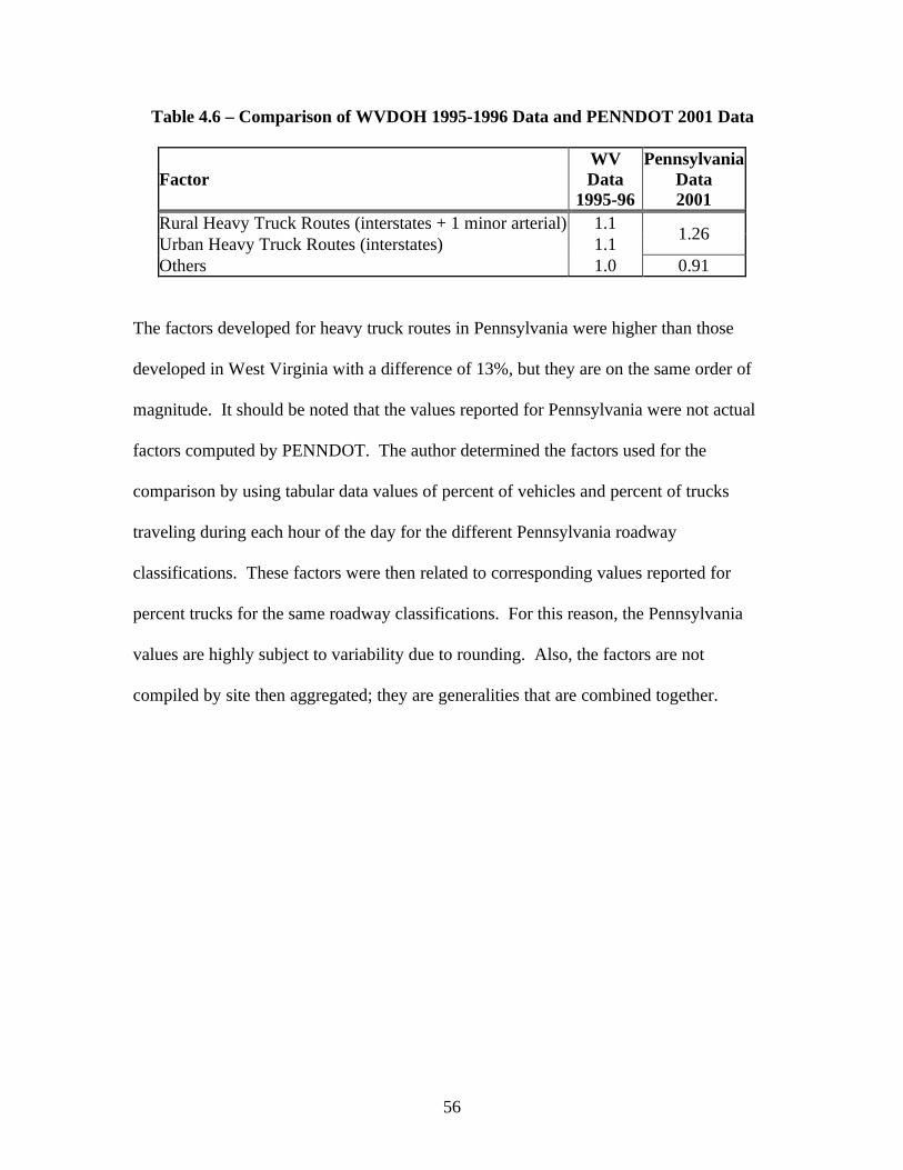
56

Table 4.6 – Comparison of WVDOH 1995-1996 Data and PENNDOT 2001 Data

FactorWVData

1995-96

PennsylvaniaData2001

Rural Heavy Truck Routes (interstates + 1 minor arterial) 1.1Urban Heavy Truck Routes (interstates) 1.1 1.26

Others 1.0 0.91

The factors developed for heavy truck routes in Pennsylvania were higher than those

developed in West Virginia with a difference of 13%, but they are on the same order of

magnitude. It should be noted that the values reported for Pennsylvania were not actual

factors computed by PENNDOT. The author determined the factors used for the

comparison by using tabular data values of percent of vehicles and percent of trucks

traveling during each hour of the day for the different Pennsylvania roadway

classifications. These factors were then related to corresponding values reported for

percent trucks for the same roadway classifications. For this reason, the Pennsylvania

values are highly subject to variability due to rounding. Also, the factors are not

compiled by site then aggregated; they are generalities that are combined together.

57

Chapter 5 CONCLUSIONS AND RECOMMENDATIONS

5.1 Conclusions

The factors developed as part of this study were derived using data collected in 1995 and

1996 from West Virginia’s 52 permanent count stations. The data provided from these

counters was reviewed and erroneous data were removed in order to ensure validity of the

raw data from the count stations.

A key limitation of the study was that about 25% of the total data from the 52 permanent

traffic recorders was either missing or in error with some sites up to 81% missing and/or

in error. A notable finding relating to the missing data occurred during the aggregation of

the factors. When determining whether or not there was a significant difference in the

factors developed by day of the month, there were too many factors missing to perform

an ANOVA analysis.

The results of this study are valid for use in West Virginia and can be utilized throughout

the state with confidence. The limitation of the factors derived by this study is that they

should only be used to adjust short-term counts performed in West Virginia. This

limitation is noted for the reason that the raw data collected at West Virginia permanent

count stations was used in the development of the factors. These factors, however, can be

applied for all roadways in West Virginia, for the permanent count stations used in the

collection of the raw data were located throughout the state. The factors developed in

this report replace those developed in 1975 to more accurately estimate current traffic

58

characteristics. Overall, the factors developed using the 52 permanent count stations in

West Virginia are consistent with those factors developed in 1975 by the WVDOH. The

changes encountered were consistent with the changing trends of truck travel.

An axle correction factor was developed as part of this study to be applied to (short-term)

axle counts. Applying an axle correction factor transforms the number of axles counted

by the short-term count into the traffic volume that traveled over the counter. Due to

variability determined by ANOVA analysis, factors were reported for each of six

different functional classification groupings. The factor developed for functional class 1

contained variability in the first quarter significant enough to necessitate that a separate

factor be reported for this quarter, with another factor representing the last three quarters

of the year. Factors for the other functional class groupings were reported as one factor

for the entire year.

Factors relating PHV to DHV were developed so that the peak hour volume experienced

on a roadway during the peak hour of the day determined by a short-term count could be

used with the factor to estimate the design hour volume. Due to the high variability

experienced within the different time groupings, the factors were reported by day of the

month for the 6 roadway functional classification groupings. Due to significant

differences with in the factors with respect to AADT, divisions were made in the groups

where AADT was a source of variation.

Factors relating percent trucks in ADT to percent trucks in peak hour were developed

based on three groupings: 1) urban heavy truck routes, 2) rural heavy truck routes, and 3)

59

other roadways. These factors are to be used to adjust the percent trucks during the peak

hour volume of the short-term counts to more accurately estimate the percentage of

trucks in the average daily traffic. Similarly, factors relating percent trucks ADT to

percent trucks in the manual count hours were developed based on the same three

groupings. These factors are to be used to adjust the percent trucks experienced during

the manual classification count hours to more accurately estimate the percentage of trucks

in the average daily traffic.

Due to changing travel patterns, particularly for commercial vehicles, and demographics

in West Virginia over the past 25 years, the factors developed in this study are meant to

replace those factors developed in 1975. The axle correction factors based on 1995-96

data are similar to those from 1975. The changes are consistent with the increased travel

of heavy trucks on the interstates that has occurred in the last 25 years. The factors

relating to axle correction were significantly different only with respect to functional

class 1 (rural interstates), namely the first quarter of the year. For this reason, one factor

was reported for the first quarter functional class 1, and one factor was reported grouping

the last three quarters of the year. All other functional classes showed no significant

difference throughout the year, thus one factor was reported for each class for the year.

The PHV to DHV factors were reported by day of the month for each functional

classification with significant variability due to AADT accounted for, rather than the

1975 method of reporting the factors by quarter and AADT alone. The factors in this

60

study were reported in this fashion due to the significant difference found while

performing ANOVA analysis.

The factors relating percent trucks in ADT to percent trucks in peak hour were somewhat

different than those reported in 1975. This difference is consistent with a greater

percentage of trucks traveling during the peak hour of the day. The factors were reported

by rural truck route, urban truck route, or other, as opposed to the 1975 method of

reporting the factors by quarter for all classes of roadways. Factors relating percent

trucks in the ADT to percent trucks in the manual count hours were not developed in

1975. This factor is to be used to adjust the percentage of trucks counted during the

manual classification count hours of 7am-10am, 11am-1pm, and 2pm-6pm.

The factors relating percent trucks in ADT to percent trucks in peak hour, and factors

relating percent trucks ADT to percent trucks in the manual count hours showed

variability only in terms of heavy and non-heavy truck routes. For this reason, factors

were reported based on the routes labeled as either rural heavy truck route, urban heavy

truck route, and all other sites combined.

The factors relating peak hour volume to design hour volume yielded many significant

differences. For this reason, the factors were reported in a more detailed fashion than the

other factors, i.e., by day of the month.

61

5.2 Recommendations

The recommendation of the research not specific to the factors that were developed

include the following:

1. Update these factors periodically to validate the current factors used and to

identify new trends that may be developing on West Virginia’s roadways.

PENNDOT for example, develops similar factors every year.

2. Inspect the permanent count stations on a regular basis and perform maintenance

and repair to the recorders to improve data quality. Troubleshooting could be

performed to identify the special causes of error.

5.3 Implementation

The factors developed herein will be immediately useful to persons analyzing traffic

count data in West Virginia. The axle correction factors are critical when machine

counts are collected with pneumatic tube counters. Furthermore, since continuous

365 day counts are available only at the permanent stations, the PHV to DHV factors

will be heavily used by highway designers, traffic engineers, and other practitioners

in the planning and design of projects statewide. Lastly, the truck percentage factors

have numerous applications, and will be used by a wide variety of practitioners. They

can be used to maximize the value of short-term truck counts in projecting total daily

truck traffic, which will be useful in both planning and design. In addition to being

distributed within the WVDOH, these factors should be made available to

consultants, MPOs, and other local entities concerned with transportation planning

62

data collection and analysis. Using the factors developed in this study, the

aforementioned agencies will be able to:

• Apply an axle correction factor to a short-term pneumatic tube axle

count to determine a more accurate traffic volume.

• Determine the design hourly volume (DHV) by measuring the peak

hour volume and applying the appropriate PHV to DHV factor.

• Determine the percent trucks in the average daily traffic on a roadway

by determining the percentage of trucks in the peak hour and applying

the appropriate % trucks in the ADT to % trucks in the peak hour

factor.

• Determine the percent trucks in the average daily traffic on a roadway

by measuring the percentage of trucks in the manual count hours and

applying the appropriate % trucks in the ADT to % trucks in the

manual count hours factor.

63

REFERENCE LIST

American Association of State Highway and Transportation Officials, AASHTOGuidelines for Traffic Data Programs, Joint Task Force on Traffic MonitoringStandards of the AASHTO Highway Subcommittee on Traffic Engineering,Washington, D.C., 1992.

American Association of State Highway and Transportation Officials, A Policy onGeometric Design of Highways and Streets, 2001, Washington, D.C., 2001.

Bureau of Transportation Planning, Annual Average Daily Traffic (AADT)Development Procedures Documentation, Michigan Department of Transportation,July 2000.

Bureau of Planning and Research, 2000 Pennsylvania Traffic Data, PennsylvaniaDepartment of Transportation, Harrisburg, PA, August 2001.

Bureau of Planning and Research, Pennsylvania Traffic Data 1998, PennsylvaniaDepartment of Transportation, Harrisburg, PA, July 1999.

Federal Highway Administration, Traffic Monitoring Guide, Office of HighwayPolicy Information, Washington, D.C., January 2001.

Sharma, Satish C; Oh, Jin Y, “Prediction of Design Hour Volume as a Function ofAmount and Nature of Travel”, ITE Journal, Volume 58, Issue 2, Washington, D.C.,1988, pages 19-24.

Traffic Analysis Section, Determination of a Truck Adjustment Factor for ATR’s,Advanced Planning Division, West Virginia Department of Highways, Charleston,WV, May 1975.

Traffic Analysis Section, Development of a Method of Estimating Design HourVolume, Advanced Planning Division, West Virginia Department of Highways,Charleston, WV, December 1975.

Traffic Analysis Section, The Relationship of the Percentage of Trucks in theAverage Daily Traffic to the Percentage of Trucks in the Peak Hour Volume,Advanced Planning Division, West Virginia Department of Highways, Charleston,WV, February 1975.

Walters, Carol H.; Poe, Christopher M., “Development of Appropriate Design-HourVolumes for Urban Freeways in Large Texas Cities”, Transportation ResearchRecord 1320, Washington, D.C., 1991, pages 32-39.

64

APPENDIX A

AXLE CORRECTION FACTOR SUMMARIES BY DAY OF THE YEAR, BY

MONTH, AND BY QUARTER

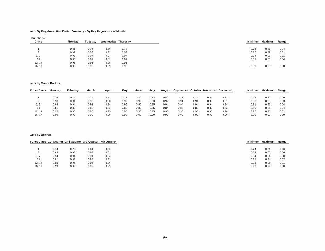
Axle By Day Correction Factor Summary - By Day Regardless of Month

FunctionalClass Monday Tuesday Wednesday Thursday Minimum Maximum Range

1 0.81 0.76 0.76 0.78 0.76 0.81 0.042 0.92 0.92 0.92 0.92 0.92 0.92 0.01

6, 7 0.95 0.94 0.94 0.94 0.94 0.95 0.0111 0.85 0.82 0.81 0.82 0.81 0.85 0.04

12, 14 0.96 0.95 0.95 0.9516, 17 0.99 0.99 0.99 0.99 0.99 0.99 0.00

Axle by Month Factors

Funct Class January February March April May June July August September October November December Minimum Maximum Range

1 0.75 0.74 0.74 0.77 0.78 0.79 0.82 0.80 0.78 0.77 0.81 0.81 0.74 0.82 0.092 0.93 0.91 0.90 0.90 0.92 0.92 0.93 0.92 0.91 0.91 0.93 0.91 0.90 0.93 0.03

6, 7 0.94 0.94 0.91 0.94 0.95 0.96 0.95 0.94 0.94 0.94 0.94 0.94 0.91 0.96 0.0411 0.81 0.80 0.82 0.82 0.82 0.82 0.85 0.84 0.83 0.82 0.83 0.83 0.80 0.85 0.04

12, 14 0.95 0.95 0.95 0.95 0.95 0.95 0.95 0.95 0.95 0.96 0.96 0.96 0.95 0.96 0.0116, 17 0.99 0.99 0.99 0.99 0.99 0.99 0.99 0.99 0.99 0.99 0.99 0.99 0.99 0.99 0.00

Axle by Quarter

Funct Class 1st Quarter 2nd Quarter 3rd Quarter 4th Quarter Minimum Maximum Range

1 0.74 0.78 0.81 0.80 0.74 0.81 0.062 0.92 0.92 0.92 0.92 0.92 0.92 0.00

6, 7 0.94 0.94 0.94 0.94 0.94 0.94 0.0011 0.81 0.83 0.84 0.83 0.81 0.84 0.02

12, 14 0.95 0.96 0.95 0.96 0.95 0.96 0.0116, 17 0.99 0.99 0.99 0.99 0.99 0.99 0.00

66

APPENDIX B

PHV TO DHV FACTOR SUMMARIES BY DAY OF THE YEAR, BY MONTH, AND

BY QUARTER

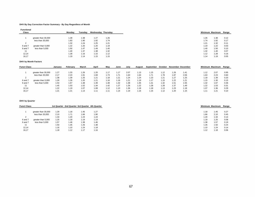
DHV By Day Correction Factor Summary - By Day Regardless of Month

FunctionalClass Monday Tuesday Wednesday Thursday Minimum Maximum Range

1 greater than 30,000 1.28 1.38 1.27 1.26 1.26 1.38 0.12less than 30,000 1.83 1.90 1.92 1.74 1.74 1.92 0.17

2 1.32 1.24 1.25 1.21 1.21 1.32 0.116 and 7 greater than 5,000 1.22 1.20 1.20 1.19 1.19 1.22 0.036 and 7 less than 5,000 1.50 1.47 1.49 1.40 1.40 1.50 0.10

11 1.40 1.37 1.38 1.32 1.32 1.40 0.0712,14 1.28 1.16 1.15 1.12 1.12 1.28 0.1616,17 1.19 1.14 1.15 1.15 1.14 1.19 0.05

DHV by Month Factors


1 greater than 30,000 1.27 1.33 1.26 1.20 1.17 1.17 2.07 1.13 1.15 1.12 1.26 1.41 1.12 2.07 0.95less than 30,000 2.17 2.23 1.91 1.69 1.73 1.71 1.63 1.63 1.71 1.78 1.87 2.06 1.63 2.23 0.60

2 1.38 1.39 1.25 1.21 1.18 1.21 1.24 1.24 1.23 1.21 1.27 1.25 1.18 1.39 0.206 and 7 greater than 5,000 1.30 1.26 1.20 1.21 1.16 1.16 1.21 1.19 1.17 1.15 1.22 1.21 1.15 1.30 0.156 and 7 less than 5,000 1.54 1.67 1.48 1.49 1.48 1.42 1.38 1.35 1.41 1.32 1.51 1.55 1.32 1.67 0.36

11 1.45 1.53 1.52 1.34 1.42 1.27 1.26 1.22 1.28 1.28 1.37 1.49 1.22 1.53 0.3112,14 1.22 1.19 1.07 1.08 1.12 1.10 1.36 1.18 1.18 1.13 1.23 1.18 1.07 1.36 0.2916,17 1.21 1.21 1.13 1.11 1.11 1.14 1.19 1.16 1.15 1.12 1.20 1.15 1.11 1.21 0.10

DHV by Quarter


1 greater than 30,000 1.29 1.18 1.45 1.27 1.18 1.45 0.27less than 30,000 2.10 1.71 1.66 1.90 1.66 2.10 0.45

2 1.34 1.20 1.24 1.24 1.20 1.34 0.146 and 7 greater than 5,000 1.25 1.18 1.19 1.19 1.18 1.25 0.086 and 7 less than 5,000 1.57 1.46 1.38 1.46 1.38 1.57 0.19

11 1.50 1.35 1.26 1.38 1.26 1.50 0.2412,14 1.16 1.10 1.24 1.18 1.10 1.24 0.1416,17 1.18 1.12 1.17 1.16 1.12 1.18 0.06

68

APPENDIX C

PERCENT TRUCKS IN ADT TO PERCENT TRUCKS IN THE PEAK HOUR

FACTOR SUMMARIES BY DAY OF THE YEAR, BY MONTH, AND BY QUARTER

Truck PH Correction Factor Summary - By Day Regardless of Month

Grouping Monday Tuesday Wednesday Thursday Minimum Maximum Range

Rural Heavy Truck Routes 1.15 1.16 1.20 1.18 1.15 1.20 0.05Urban Heavy Truck Routes 1.19 1.21 1.18 1.21 1.18 1.21 0.03Other 1.08 1.13 1.08 1.09 1.08 1.13 0.05

Truck PH by Month Factors

Grouping January February March April May June July August September October November December Minimum Maximum Range

Rural Heavy Truck Routes 1.17 1.17 1.18 1.19 1.18 1.16 1.18 1.17 1.15 1.17 1.17 1.17 1.15 1.19 0.04Urban Heavy Truck Routes 1.18 1.20 1.23 1.24 1.21 1.19 1.14 1.19 1.26 1.22 1.15 1.18 1.14 1.26 0.12Other 1.09 1.10 1.08 1.07 1.19 1.10 1.09 1.14 1.09 1.10 1.10 1.20 1.07 1.20 0.13

Truck PH by Quarter

Grouping 1st Quarter 2nd Quarter 3rd Quarter 4th Quarter Minimum Maximum Range


70

APPENDIX D

PERCENT TRUCKS IN ADT TO PERCENT TRUCKS IN THE MANUAL COUNT

HOUR FACTOR SUMMARIES BY DAY OF THE YEAR, BY MONTH, AND BY

QUARTER

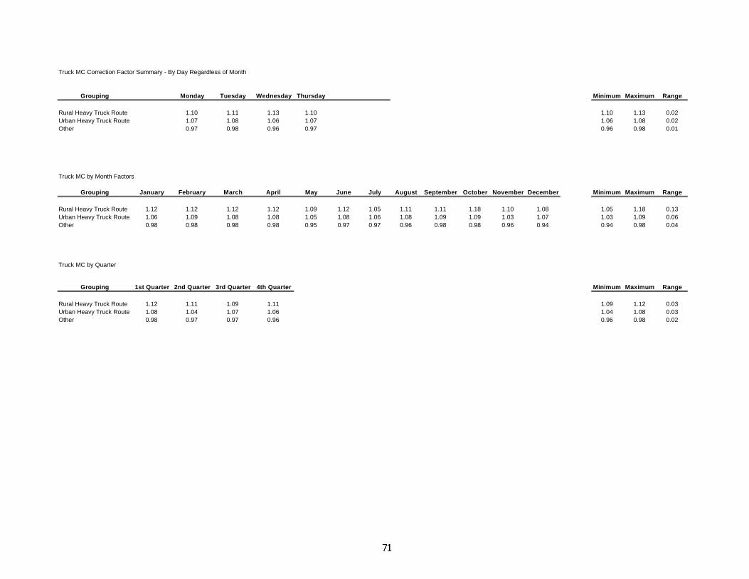
Truck MC Correction Factor Summary - By Day Regardless of Month

Grouping Monday Tuesday Wednesday Thursday Minimum Maximum Range

Rural Heavy Truck Route 1.10 1.11 1.13 1.10 1.10 1.13 0.02Urban Heavy Truck Route 1.07 1.08 1.06 1.07 1.06 1.08 0.02Other 0.97 0.98 0.96 0.97 0.96 0.98 0.01

Truck MC by Month Factors


Rural Heavy Truck Route 1.12 1.12 1.12 1.12 1.09 1.12 1.05 1.11 1.11 1.18 1.10 1.08 1.05 1.18 0.13Urban Heavy Truck Route 1.06 1.09 1.08 1.08 1.05 1.08 1.06 1.08 1.09 1.09 1.03 1.07 1.03 1.09 0.06Other 0.98 0.98 0.98 0.98 0.95 0.97 0.97 0.96 0.98 0.98 0.96 0.94 0.94 0.98 0.04

Truck MC by Quarter


Rural Heavy Truck Route 1.12 1.11 1.09 1.11 1.09 1.12 0.03Urban Heavy Truck Route 1.08 1.04 1.07 1.06 1.04 1.08 0.03Other 0.98 0.97 0.97 0.96 0.96 0.98 0.02

72

APPENDIX E

FACTORS DEVELOPED USING ONLY FRIDAY,

SATURDAY, AND SUNDAY DATA

Axle By Day Correction Factor Summary - By Day Regardless of Month

FunctionalClass Sunday Monday Tuesday Wednesday Thursday Friday Saturday Minimum Maximum Range

1 0.88 0.84 0.88 0.84 0.88 0.042 0.97 0.93 0.97 0.93 0.97 0.04

6, 7 0.98 0.95 0.98 0.95 0.98 0.0311 0.89 0.87 0.90 0.87 0.90 0.03

12, 14 0.98 0.96 0.98 0.96 0.98 0.0316, 17 1.00 0.99 1.00 0.99 1.00 0.00

Axle by Month Factors


1 0.81 0.82 0.85 0.86 0.87 0.88 0.89 0.89 0.87 0.87 0.89 0.89 0.81 0.89 0.082 0.95 0.94 0.94 0.95 0.96 0.96 0.96 0.96 0.95 0.96 0.96 0.96 0.94 0.96 0.02

6, 7 0.96 0.97 0.95 0.97 0.97 0.98 0.97 0.97 0.97 0.97 0.97 0.97 0.95 0.98 0.0311 0.86 0.86 0.89 0.89 0.89 0.89 0.90 0.90 0.89 0.88 0.89 0.89 0.86 0.90 0.05

12, 14 0.98 0.97 0.96 0.97 0.98 0.97 0.97 0.97 0.98 0.98 0.98 0.98 0.96 0.98 0.0216, 17 1.00 1.00 1.00 1.00 1.00 0.99 0.99 0.99 0.99 1.00 1.00 1.00 0.99 1.00 0.00

Axle by Quarter


1 0.83 0.87 0.89 0.88 0.83 0.89 0.062 0.95 0.96 0.96 0.96 0.95 0.96 0.00

6, 7 0.96 0.97 0.97 0.97 0.96 0.97 0.0111 0.87 0.89 0.90 0.89 0.87 0.90 0.03

12, 14 0.97 0.98 0.97 0.98 0.97 0.98 0.0116, 17 1.00 1.00 0.99 1.00 0.99 1.00 0.00

Friday Saturday-Sunday

Functional Class 1st Quarter Rest of Year Entire Year Functional Class 1st Quarter Rest of Year Entire Year1 0.80 0.85 1 0.84 0.892 0.93 2 0.97

6, 7 0.95 6, 7 0.9811 0.87 11 0.90

12, 14 0.96 12, 14 0.9816, 17 0.99 16, 17 1.00

PHV-DHV Factor Summary - By Day Regardless of Month

FunctionalClass Sunday Monday Tuesday Wednesday Thursday Friday Saturday Minimum Maximum Range

1 1.48 1.35 1.67 1.35 1.67 0.322 1.99 1.53 2.02 1.53 2.02 0.48

6, 7 1.43 1.17 1.41 1.17 1.43 0.2611 1.49 1.21 1.52 1.21 1.52 0.31

12, 14 1.67 1.09 1.63 1.09 1.67 0.5816, 17 1.53 1.12 1.42 1.12 1.53 0.41

PHV-DHV by Month Factors


1 2.14 1.97 1.42 1.32 1.37 1.29 1.35 1.16 1.30 1.41 1.44 1.79 1.16 2.14 0.982 2.61 3.27 2.01 1.96 1.69 1.67 1.66 1.71 1.66 1.62 1.78 1.88 1.62 3.27 1.65

6, 7 1.69 1.51 1.31 1.30 1.26 1.27 1.26 1.27 1.27 1.23 1.34 1.39 1.23 1.69 0.4611 1.82 1.90 1.45 1.32 1.36 1.23 1.16 1.18 1.31 1.27 1.30 1.53 1.16 1.90 0.74

12, 14 1.90 1.61 1.25 1.32 1.37 1.35 1.43 1.35 1.33 1.33 1.39 1.37 1.25 1.90 0.6616, 17 1.57 1.21 1.10 1.29 1.26 1.31 1.39 1.40 1.36 1.33 1.46 1.43 1.10 1.57 0.47

PHV-DHV by Quarter


1 1.88 1.33 1.25 1.55 1.25 1.88 0.632 2.34 1.71 1.68 1.76 1.68 2.34 0.67

6, 7 1.53 1.27 1.26 1.32 1.26 1.53 0.2611 1.76 1.30 1.22 1.37 1.22 1.76 0.55

12, 14 1.68 1.38 1.37 1.36 1.36 1.68 0.3216, 17 1.32 1.29 1.38 1.41 1.29 1.41 0.12

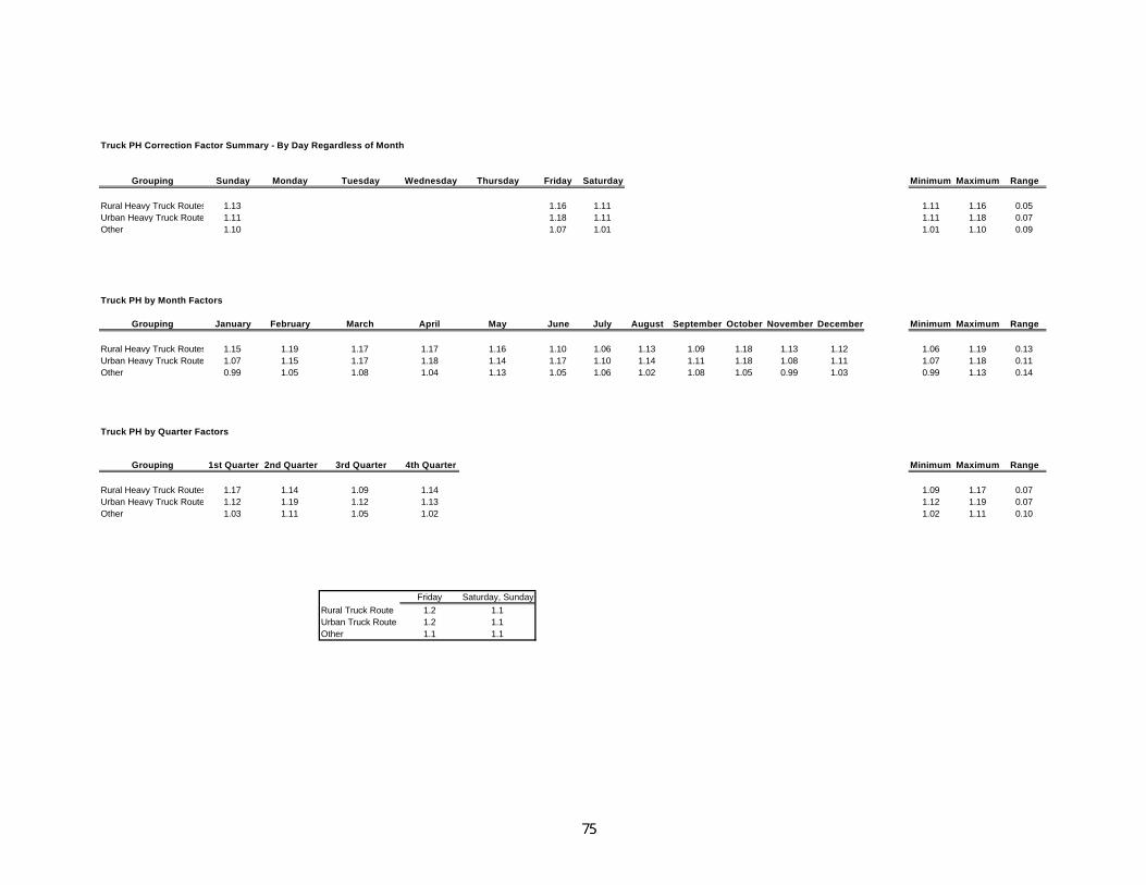
Truck PH Correction Factor Summary - By Day Regardless of Month

Grouping Sunday Monday Tuesday Wednesday Thursday Friday Saturday Minimum Maximum Range

Rural Heavy Truck Routes 1.13 1.16 1.11 1.11 1.16 0.05Urban Heavy Truck Routes 1.11 1.18 1.11 1.11 1.18 0.07Other 1.10 1.07 1.01 1.01 1.10 0.09

Truck PH by Month Factors



Truck PH by Quarter Factors



Friday Saturday, SundayRural Truck Route 1.2 1.1Urban Truck Route 1.2 1.1Other 1.1 1.1

Truck MC Correction Factor Summary - By Day Regardless of Month

Grouping Sunday Monday Tuesday Wednesday Thursday Friday Saturday Minimum Maximum Range

Rural Heavy Truck Routes 1.09 1.07 1.06 1.06 1.09 0.03Urban Heavy Truck Routes 1.03 1.04 1.03 1.04 0.00Other 0.99 0.95 0.97 0.95 0.99 0.04

Truck MC by Month Factors



Truck MC by Quarter



Friday, Saturday, and Sunday

Rural Truck Route 1.1Urban 1.0Other 1.0

use of west virginia permanent traffic recorder data to

Documents