Use of Nonsymmetric

Algebraic Operators in a Semi-Implicit MHD Advance

Carl Sovinec and Hao Tian Department of Engineering Physics, University

of Wisconsin-Madison

2003 International Sherwood Fusion Theory Conference

April 28-30, 2003

Corpus Christi, Texas

OBJECTIVES

• Develop a semi-implicit MHD algorithm where the time-step is not severely restricted by equilibrium flow.

• Compare the performance of symmetric and nonsymmetric semi-implicit operators for MHD.

• Investigate the effectiveness of a fourth-order semi-implicit operator for the Hall term in two-fluid systems.

OUTLINE

I. Background

A. Semi-implicit MHD

B. Solving nonsymmetric systems

II. Advection

III. Two-fluid advance

IV. MHD reformulation

V. Conclusions

BACKGROUND

The basic semi-implicit algorithm for hyperbolic systems can be described as a leap-frog scheme with an implicit linear operator for stabilizing the advance at arbitrarily large time-step. • The leap-frog aspect makes the integration symplectic. • The linear operator acts on the rate of change to stabilize

through numerical dispersion [Caramana, JCP 96, (1991)]. The semi-implicit method for the simple linear system

xac

tb

xbc

ta

∂∂

−=∂∂

∂∂

−=∂∂

can be derived by the method of differential approximation [Carmana], arriving at

( )

xatcbb

xbtcaa

xtsc

nnn

nnn

∂∂

∆−=−

∂∂

∆−=−

∂

∂∆−

++

+

11

12

2221

where superscripts indicate the time-step index, and s is a dimensionless coefficient.

• After applying the Fourier transform in space, we may find the eigenvalue of the numerical advance and the value of s needed for numerical stability:

Substituting

n

k

kk

n

k

kba

ba

=

+

ˆˆ

ˆˆ 1

λ

into the time-discrete equations leads to

( )

)1(2

4411 2

242

k

kkkk

s

s

ξ

ξξξλ

+

−−±−=

where k is the wavenumber, and tckk ∆≡ξ . The advance is both stable and free of numerical dissipation (|λk|=1) for all values of ∆t when s≥1/4.

• The absence of numerical dissipation makes the basic

algorithm well suited for macroscopic modeling of high-temperature plasmas.

• Accuracy at large time-step is largely determined by how well the eigenpairs of the semi-implicit operator represent the normal modes of the system [Schnack, et al., JCP 70, 330 (1987)].

The semi-implicit algorithm has been successfully applied to nonlinear fusion MHD problems with codes like DEBS [Schnack], XTOR [Lerbinger and Luciani, JCP 97, 444 (1991)], and NIMROD [Glasser, et al., PPCF 41, A747 (1999)]. • The semi-implicit operators in XTOR and NIMROD are based

on the linear ideal MHD force operator for accuracy. Thus, the flow velocity advance for linear computations with a static equilibrium appears as

( )( ) ( )n

nnnn

pt

ttts

∇∆−

×∆+××∇∆=−∆− + BJBBVVL 000

12 1µ

ρ

where

( ) ( )[ ] (

( )VV

BVJBBVVL

⋅∇+∇⋅∇+

××∇×+×××∇×∇≡

00

00000

1

pp γµ

)

• A Laplacian operator with a small coefficient is added to L to

stabilize waves in nonlinear conditions.

A linear computation of an internal kink mode for a cylindrical tokamak equilibrium demonstrates the algorithm’s accuracy at large time-step. [∆t is varied from 103 to >104 times the explicit limit.]

r/a

q P

0 0.25 0.5 0.75 1

0.6

0.8

1

1.2

1.4

1.6

1.8

0.2

0.3

0.4

0.5

0.6

0.7

0.8

0.9

1

P/r=

0

Equilibrium Profiles

( )( )( )( )

1Pm

52

10

/216.0)(

/75.01)(

%10,52

62

0

2

20

=

==

==

+=

−=

==

=

AA

r

r

vL

a

arrq

arPrP

aL

πτ

ηµτ

βπ

R

Z

1 1.5 2 2.5 3-1

-0.75

-0.5

-0.25

0

0.25

0.5

0.75

1

γ0 ∆t

γ com

pute

dτ A

0 0.1 0.2 0.3 0.4 0.5

0.0456

0.0458

0.046

0.0462

0.0464

0.0466

0.0468

0.047

Linear Eigenfunction, ReV Growth Rate Convergence

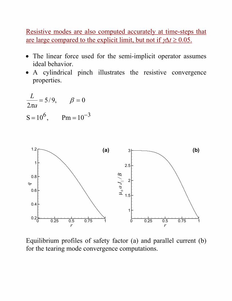
Resistive modes are also computed accurately at time-steps that are large compared to the explicit limit, but not if γ∆t ≥ 0.05. • The linear force used for the semi-implicit operator assumes

ideal behavior. • A cylindrical pinch illustrates the resistive convergence

properties.

36 10Pm,10S

0,9/52

−==

== βπaL

r

µ 0a

J ||/B

0 0.25 0.5 0.75 1

1

1.5

2

2.5

3 (b)

r

q

0 0.25 0.5 0.75 10.2

0.4

0.6

0.8

1

1.2 (a)

Equilibrium profiles of safety factor (a) and parallel current (b) for the tearing mode convergence computations.

γ0 ∆t

γτ A

0 0.025 0.05 0.075 0.1 0.1255.9E-04

6.0E-04

6.1E-04

6.2E-04

6.3E-04

6.4E-04

6.5E-04forwardcentered

Computed growth rate scanning time-step for the tearing computation. The two curves compare forward and centered temporal differencing of the diffusive terms. • At γ0∆t=0.064, the time-step is >105 times the explicit stability

limit. • However, accuracy for this nonideal computation suffers at

γ0∆t values that are roughly five times smaller than in the ideal computation.

While small values of resistivity do not pose severe limitations on time-step for the traditional semi-implicit approach, other ‘nonideal’ effects such as advection and two-fluid terms can be challenging. • Flow is typically treated through explicit terms. Upwinding or

predictor/corrector steps are needed to stabilize advection, and the Courant-Friedrich-Lewy (CFL) condition [Mathematische Annalen 100, 32 (1928)] must be obeyed. • For a flow of 1% vA, the time-step may be ~100 times

smaller than that needed for accuracy in a typical NIMROD computation without flow.

• Centering of the wave contributions is important during the predictor step to avoid instability at small dissipation. [Lionello et al., JCP 152, 346 (1999)]

• The dispersive nature of waves in the two-fluid model requires

a fourth-order differential operator for a straightforward semi-implicit approach. [Harned and Mikic, JCP 83, 1 (1989)] • Fourth-order operators may be difficult or impossible to

implement, depending on the spatial representation. Can we extend the basic semi-implicit approach to address these issues without sacrificing accuracy and efficiency by using nonsymmetric operators??

We have recently updated a coupling between NIMROD and SNL’s AZTEC (www.cs.sandia.gov/CRF/aztec1.html) parallel linear solver in order to explore the use of nonsymmetric operators. • NIMROD’s conjugate gradient (CG) solver was developed for

symmetric- and Hermitian-positive-definite matrices only. • Software written by Steve Plimpton of SNL for the original

version of NIMROD arranged linear and bilinear finite element data into a form suitable for AZTEC. Newer versions of NIMROD use Lagrange polynomials of arbitrary degree. [Sovinec, et al., “Nonlinear magnetohydrodynamics simulation using high-order finite elements,” submitted to JCP]

• Tests using AZTEC’s solver for a linear tearing-mode computation in toroidal geometry (mesh and q profile below) with biquartic elements and the unmodified NIMROD time-advance provide confidence in the implementation.

R

Z

1 1.5 2 2.5

-1

-0.5

0

0.5

1

Ψ1/2

q

0 0.25 0.5 0.75 1

2

3

4

5

6

7

8

The AZTEC library was able to solve our HPD semi-implicit operator at large ∆t with either CG or generalized minimum residual (GMRES) methods, but the computational cost of using the nonsymmetric solver is considerable. Comparison of solver performance for a 32×32 mesh of biquartic

finite elements with ∆t=4 wave transit times.

Solver Preconditioner Subdomain Solve Ave. Vel. Its. Solve Time/Step

nim-cg nr=10k

line Jacobi - 2152 53.1

nim-cg nr=50 line Jacobi - 2819 69.5

az-cg Jacobi point block Jacobi 21505 144 az-cg dom_decomp

0 icc 1 rthresh=1.15 6252 179

gmr ksp=500 dom_decomp

2 ilut 6 dr=1.e-6

rthresh=1.2 5757 1157

gmr ksp=1k dom_decomp 2

ilut 6 dr=1.e-6 rthresh =1.2

4636 1327

gmr ksp=1k dom_decomp 0

ilut 6 dr=1.e-6 rthresh =1.2

7053 1331

gmr ksp=200 dom_decomp 0

ilut 4 drop=10-5 rthresh=1.15

no conv in 10k

• Orthogonalization of direction vectors adds to the computation

time of GMRES. • If new temporal algorithms lead to nonsymmetric systems that

are equally difficult to solve, they will have to allow accurate computation at significantly larger time-steps to be cost-effective.

ADVECTION Time-step limitations imposed by explicit advection are an impediment to running numerical simulations at realistic parameters. • Studies of tokamak internal kink modes with sheared poloidal

flow that approaches the poloidal sound speed [Kissick, PoP 8, 174 (2001)] were motivated by the Electric Tokamak experiment at UCLA [Taylor, “Initial plasmas in ET at low magnetic fields,” IAEA, Sorento, Italy (2000)].

• We may impose a similar poloidal flow profile on the cylindrical tokamak mode described above.

r

V 0/v

A

0 0.25 0.5 0.75 10

0.005

0.01

0.015

Sheared poloidal flow profile for the cylindrical tokamak test. The poloidal sound speed is ~ 0.03 vA.

• With NIMROD’s explicit predictor/corrector method for flow, the computation runs successfully at S=2×105 and Pm=1. However, with a 16×16 mesh of biquadratic finite elements, the time-step is restricted to 0.06 τA (γ0∆t=0.003), two orders of magnitude smaller than the ∆t-value required for accuracy without flow.

t / τA

Re

Bφ

n=1

atpr

obe

0 50 100 150

-2E-10

-1E-10

0

1E-10

2E-10

3E-10

4E-10

5E-10

R

Z

1 1.5 2 2.5 3-1

-0.75

-0.5

-0.25

0

0.25

0.5

0.75

1

Magnetic Signal History Eigenfunction, ReV

• The predictor/corrector advection also requires an increase in the coefficient for the symmetric semi-implicit operator. [Lionello]

The numerical stability properties of the predictor/corrector (p/c) advection combined with the HPD semi-implicit operator can be understood by analyzing the simple wave system with uniform flow added. With u as the imposed flow velocity, the simple system becomes:

xac

xbu

tb

xbc

xau

ta

∂∂−

∂∂−=

∂∂

∂∂

−∂∂

−=∂∂

• The semi-implicit p/c algorithm for this system is

( )

( ) ( )

( )x

atcx

bffbtubb

xatc

xbtubb

xbtc

xaffatuaa

xtsc

xbtc

xatuaa

xtsc

nnnn

nnn

nnnn

nnn

∂∂

∆−∂

−+∂∆−=−

∂∂

∆−∂

∂∆−=−

∂∂

∆−∂

−+∂∆−=−

∂

∂∆−

∂∂

∆−∂

∂∆−=−

∂

∂∆−

+∗+

+∗

∗+

∗

11

1

12

222

2

222

)1(

)1(1

1

ω

ω

where f is a centering parameter for the p/c method, and ω affects the amplitude of the wave terms in the predictor steps.

• Performing a numerical analysis that is similar to what was done for the system without flow, we arrive at the following dispersion relation for the eigenvalue (λ) of the time-step operation. [Wavenumber subscripts are suppressed, but the eigenvalue is for a given k-value.]

( )[ ]

( ) [ ] 011

111

1

22

2

222

2

2

=+×

++

+−

++−×

++

++−

ωηξ

ωηξ

ξλ

ηηλξ

ηξ

ηλ

fis

fis

fis

fs

i

where tck∆≡ξ and tuk∆≡η .

• As shown in Ref. [Lionello], it is necessary to have fω=1/2 and

to increase s from the value of 1/4 in order to assure stability at large ξ.

s=1/4 s=1/2

η

η

ξ ξ

s=1

η

ξ

The regions of numerical stability, |λ|≤1, for the semi-implicit p/c algorithm are shown in black for the indicated values of the semi-implicit coefficient, s.

Implicit Advection

An alternative approach is to treat advection implicitly while maintaining the rest of the semi-implicit advance. • Since the advection operator (V0⋅∇) is not self-adjoint, the

resulting matrices will be nonsymmetric, requiring AZTEC or another nonsymmetric solver.

• It is not readily apparent that this approach is numerically stable at large time-step, since it is not formulated by centering all terms at the same time-level. [The leap-frog character is retained.] Furthermore, the advection-augmented semi-implicit operator has complex eigenvalues.

Here the numerical algorithm applied to the simple hyperbolic system with flow is described by

( ) ( )

( )x

atcx

bffbtubb

xbtc

xaffatuaa

xtsc

nnnnn

nnnnn

∂∂

∆−∂

−+∂∆−=−

∂∂

∆−∂

−+∂∆−=−

∂

∂∆−

+++

++

111

11

2

222

)1(

)1(1

where f is now the implicit centering for advection.

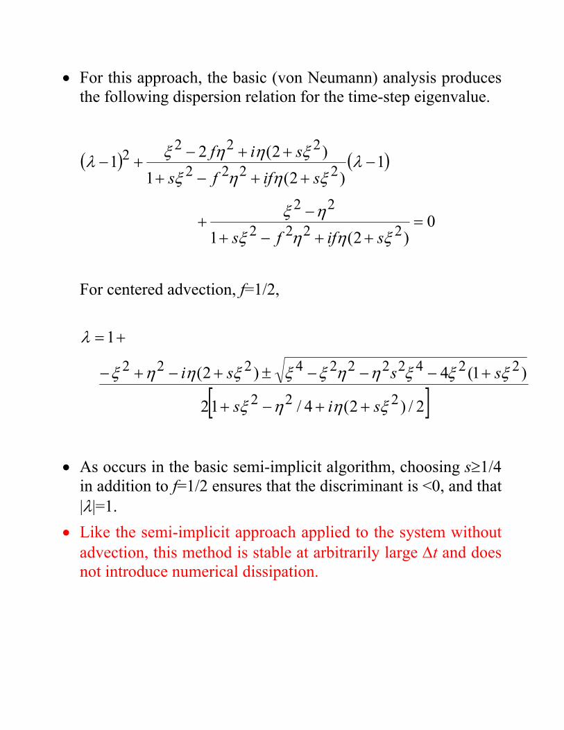
• For this approach, the basic (von Neumann) analysis produces the following dispersion relation for the time-step eigenvalue.

( ) ( )

0)2(1

1)2(1

)2(21

2222

22

2222

2222

=++−+

−+

−++−+

++−+−

ξηηξηξ

λξηηξ

ξηηξλ

siffs

siffssif

For centered advection, f=1/2,

[ ]2/)2(4/12

)1(4)2(

1

222

22422224222

ξηηξ

ξξξηηξξξηηξ

λ

sis

sssi

++−+

+−−−±+−+−

+=

• As occurs in the basic semi-implicit algorithm, choosing s≥1/4

in addition to f=1/2 ensures that the discriminant is <0, and that |λ|=1.

• Like the semi-implicit approach applied to the system without advection, this method is stable at arbitrarily large ∆t and does not introduce numerical dissipation.

This implicit advection method has been implemented for equilibrium flow (plasma rotation) in NIMROD using the AZTEC library for solution of the nonsymmetric linear systems. • A simple test evolves magnetoacoustic waves in a periodic

box, where the medium is translating with respect to the lab (computational mesh) frame. • Selecting Vz=2×106 m/s, c=4×105 m/s, Lz=1 m, standing

waves in the fluid frame appear as streaks in the plotted contours of B⊥.

Z (m)

t(s)

0 0.25 0.5 0.75 10

1E-06

2E-06

3E-06

4E-06

Fluid Motion

Contours of the perpendicular component of B in the Z-t plane.

• In this computation, there are 16 quadratic elements in the

Z-direction, and ∆t=1×10-7, so Vzk ∆t ≅ 20.

• A simulation of the cylindrical internal kink mode subject to rigid poloidal rotation has also been successful with a 12×12 mesh of biquadratic elements.

0

5

10

15

20

t/τA

12

3R

-10

1Z

Linear velocity solution for the internal kink with rigid rotation shown at six successive time steps. The time-steps of 4 τΑ exceed the CFL condition by a factor of 3.5. • This computation is encouraging, but the nonsymmetric matrix

proved difficult for the solver library. The symmetric part is ill-conditioned, and the advection makes the eigenvalues complex. Convergence has not been achieved for computations with greater mesh resolution.

Time-Split Advection

Another approach is to advance all fields from the wave terms, then update for advection. This is similar to an Arbitrary Lagrangian Eulerian (ALE) approach, but the Lagrangian mesh distortion is not applied. • Although the time-splitting makes the advance only first-order

accurate, the matrices for the separate implicit advective steps are easier to solve than the matrix for the combined semi-implicit-advective operator discussed above.

• For the simple hyperbolic system with flow, the time-split method is described by

( )

( )

( )x

bffbtubb

xaffatuaa

xatcbb

xbtcaa

xtsc

nn

nn

n

nn

∂−+∂

∆−=−

∂−+∂

∆−=−

∂∂

∆−=−

∂∂

∆−=−

∂

∂∆−

∗+∗+

∗+∗+

∗∗

∗

)1(

)1(

1

11

11

2

222

• A von Neumann analysis predicts numerical stability

provided that both the wave and advective steps are stable.

This approach has been implemented in NIMROD in two forms. One uses an implicit advance for the advection step, and the other uses the p/c method with subcycling to relax the CFL condition in the Lagrangian-like step. • The implementations will reproduce simple waves in a

translating reference frame. • However, this approach has not proven successful for rigid

rotation of the cylindrical internal kink mode. With either implementation, the computation will run a number of time-steps and then degenerate into a faster growing numerical instability with oscillations at the smallest wavelength supported by the spatial representation.

t / τA

γτ A

0 10 20 30 40

-1

-0.5

0

0.5

1

1.5

R

Z

1 1.5 2 2.5 3-1

-0.75

-0.5

-0.25

0

0.25

0.5

0.75

1

Instantaneous growth rate and contours of temperature resulting in the linear computation of the cylindrical tokamak with rigid rotation and the split advection scheme.

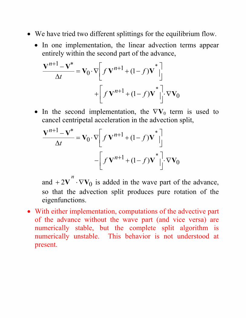
• We have tried two different splittings for the equilibrium flow. • In one implementation, the linear advection terms appear

entirely within the second part of the advance,

01

10

1

)1(

)1(

VVV

VVVVV

∇⋅

−++

−+∇⋅=

∆−

∗

∗

+

+∗+

ff

fft

n

nn

• In the second implementation, the ∇V0 term is used to cancel centripetal acceleration in the advection split,

01

10

1

)1(

)1(

VVV

VVVVV

∇⋅

−+−

−+∇⋅=

∆−

∗

∗

+

+∗+

ff

fft

n

nn

and is added in the wave part of the advance, so that the advection split produces pure rotation of the eigenfunctions.

02 VV ∇⋅+n

• With either implementation, computations of the advective part of the advance without the wave part (and vice versa) are numerically stable, but the complete split algorithm is numerically unstable. This behavior is not understood at present.

R

Z

1 1.5 2 2.5 3-1

-0.5

0

0.5

1t/τA=0

R

Z

1 1.5 2 2.5 3-1

-0.5

0

0.5

1t/τA=1.6

R

Z

1 1.5 2 2.5 3-1

-0.5

0

0.5

1t/τA=3.2

R

Z

1 1.5 2 2.5 3-1

-0.5

0

0.5

1t/τA=3.2

R

Z

1 1.5 2 2.5 3-1

-0.5

0

0.5

1t/τA=1.6

R

Z

1 1.5 2 2.5 3-1

-0.5

0

0.5

1t/τA=0

Evolution of linear flow pattern

from V0⋅∇V+V⋅∇V0 only. Evolution of linear flow patternfrom V0⋅∇V-V⋅∇V0 only

TWO-FLUID ADVANCE Modeling electron fluid effects in simulations of nonlinear macroscopic dynamics is computationally challenging, since it leads to greater ranges of time and space scales relative to resistive MHD, which is already very stiff in many conditions of interest. • Different numerical methods for modeling the general two-

fluid system (without drift orderings) over MHD time-scales can be categorized as ‘Ampere-centric’ or ‘Faraday-centric’ (or more commonly ‘two-fluid’ vs. ‘extended MHD’).

• To describe their differences, consider a hydrogen plasma in the limit of zero pressure. The species momentum equations can be expressed as

BJEJJJ ×+=

⋅∇+

∂∂

sss

sss

sssss

mq

mqn

qnt

2, s=i,e

A numerical computation of slow macroscopic behavior will need to take time-steps that are far larger than the fast time scales over which both electron and ion motion equilibrate electric field forces. Thus, some type of implicit or semi-implicit scheme is needed for advancing motions and E in a consistent way.

An Ampere-centric approach is used in the Quiet Implicit PIC (QIP) algorithm [D. Barnes et al., 1996 Sherwood Conference] and is related to direct implicit PIC computations. The numerical advance is based on an implicit conductivity function, which is similar to the analytical conductivity tensor derived for cold plasma waves.

• Linearize with J0=0 for the point of illustration, and create a

time-centered advance for all but the advective terms.

( )

+⋅∇∆+

×Ω∆

−+∆

+=×Ω∆

+ +++

ss

sn

sn

ss

nss

nnsssn

sn

ssn

s

qnt

tmqntt

00

2221

211

JJJJ

JEEJJJ

where sss mq /0B≡Ω . This equation can be arranged to find Js

n+1 in terms of En+1 and explicit terms.

ermsexplicit t

2424/11 1

22

221

+

∆

⋅ΩΩ

∆+×Ω

∆−

Ω∆+= ++ n

sss

ssss

ns m

qntttt

EIJ

• The two species equations can be added to produce the

function Jn+1(En+1).

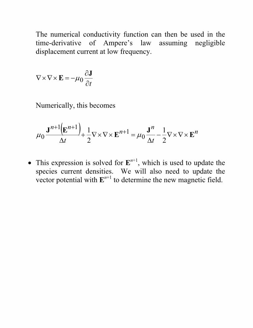
The numerical conductivity function can then be used in the time-derivative of Ampere’s law assuming negligible displacement current at low frequency.

t∂∂

−=×∇×∇JE 0µ

Numerically, this becomes

( ) nn

nnn

ttEJEEJ

×∇×∇−∆

=×∇×∇+∆

+++

21

21

01

110 µµ

• This expression is solved for En+1, which is used to update the

species current densities. We will also need to update the vector potential with En+1 to determine the new magnetic field.

The Faraday-centric class of methods is the more familiar extension of MHD to use a generalized Ohm’s law. • With the assumption of quasineutrality (built into the Ampere-

centric approach by eliminating displacement current), the pair of species current equations are equivalent to the following equations for the center-of-mass flow velocity and generalized Ohm’s law.

( )

+⋅∇+∂∂

+×+×−=

×=

∇⋅+

∂∂

VJJVJBJBVE

BJVV

tne

t

p2

0

11ωε

ρ

• Here, the relation for E is substituted into Faraday’s law, so

unlike the Ampere-centric approach, E is not a fundamental quantity for the numerical computation.

• Semi-implicit methods are possible with the Faraday-centric approach to the two-fluid system [Harned and Mikic, JCP 83, 1 (1989)]. The flow velocity is advanced separately from the magnetic field using the semi-implicit operators described in the background section. However, the magnetic advance also requires some type of implicit operator to stabilize whistler waves at large time-step.

Semi-Implicit Hall

• Focusing on the magnetic field advance from the Hall term alone, we have a simple evolution equation from Faraday’s law.

××−∇=

∂∂ BJB

net1

A time-centered linear advance for small J0 is

××∇

∆×∇−

=

××∇

∆×∇+ ++

00

01

0

1

)(2

)(2

BB

BBBB

n

nnn

net

net

µ

µ

• The linear differential operator is not self-adjoint in this form,

so a discrete version would yield a nonsymmetric matrix.

• A self-adjoint operator can be formed by making a second-order wave equation from the relevant magnetic advance. This is analogous to forming the linear MHD force operator by eliminating the equations for B and p.

( )

×

××∇×∇×∇×∇=

×

∂∂

×∇×−∇=∂

∂

0000

002

2

11

1

BBB

BBB

nene

tnet

µµ

µ

Using this operator in a semi-implicit advance then appears as

( ) rhsnet

net

=

×

×∆×∇

∆×∇×∇

∆×∇−∆ 00

00BBBB

µµ

This is similar to the Hall semi-implicit operator recommended in Ref. [Harned and Mikic].

• Implementation with a finite element spatial representation requires a weak form with integration by parts to reduce the order of continuity required from the solution space. Hence, we need to satisfy an equation of the form

( ) ( ) rhsnet

netd

d

=

××∇

∆×∇⋅

×∆×∇

∆×∇+

∆⋅

∫

∫

00

00

BABBx

BAx

µµ

for all appropriate test functions A. With Lagrange polynomials as the finite element basis functions, derivatives are not continuous at element boundaries, so the second term in the above equation is not integrable. To remedy this, we may introduce an auxiliary field and corresponding equation in the system.

( )

( ) 0BBgxfgx

BAfxBAx

=

×∆×∇

∆⋅×∇−⋅

=

××∇

∆⋅×∇+∆⋅

∫∫

∫∫

00

00

netdd

rhsnetdd

µ

µ

for all appropriate test functions A and g.

• We are presently implementing the fourth-order Hall semi-implicit operator and will also implement a linear implicit Hall advance for comparison.

• Both implementations will require use of the nonsymmetric

solver library.

MHD REFORMULATION It is possible that reformulating the MHD semi-implicit advance without the eliminating ∆p and ∆B in the flow velocity advance will lead to a better conditioned system. It may also have favorable numerical properties. • The related time-discrete linear equations are

( )

( )( )

( ) 0

1

1

00

0

000

000

=∆⋅∇+∇⋅∆∆+∆

=×∆×∇∆−∆

∇∆−×∆+××∇∆

=∆∇+∆×∆−×∆×∇∆−∆

VV

0BVB

BJBB

BJBBV

pptsp

ts

pttt

pststs

nnn

γ

µ

µρ

While this system is analytically equivalent to the semi-implicit advance described in the background discussion, having ∆B and ∆p as discretized fields will have different numerical properties. In finite element form, this version is a mixed representation.

• Here the terms appearing on the lhs have the same spatial representation as the explicit contributions on the rhs.

• The resulting matrix will have complex eigenvalues, but the range of eigenvalues magnitudes will be much smaller. Thus, it may be easier to solve.

• This representation may allow introducing resistive diffusion in the linear part of the velocity advance.

CONCLUSIONS • While the leap-frog-based semi-implicit method has proven

effective for macroscopic simulations requiring large time-steps, nonideal conditions detract from its performance. This motivates considering additional nonsymmetric contributions in implicit terms.

• Numerical analysis of the unsplit implicit advection and test results show that it is possible to introduce non-self-adjoint operators in a semi-implicit algorithm without losing numerical stability.

• The tests also demonstrate that modifying the ill-conditioned MHD operator so that the eigenvalues are perturbed from the real axis makes a linear system that is much more difficult to solve. Better use of available linear system software options may help.

• A more detailed analysis of the split advection approach is required to explain its numerically unstable behavior.

• Multiple formulations of a semi-implicit Hall advance are possible and are presently under development.

• A ‘mixed’ formulation of the MHD semi-implicit operator may have several benefits and will also be investigated.

This poster will be made available on the NIMROD Team web site, http://nimrodteam.org.