use of machine learning algorithms in vessel performance
TRANSCRIPT

Use of machine learning algorithms in vessel performance monitoring Adeline Crystal John Suresh Kumar
Master’s Thesis
DTU Mechanical EngineeringDepartment of Mechanical Engineering

U S E O F M A C H I N E L E A R N I N GA L G O R I T H M S I N V E S S E L
P E R F O R M A N C E M O N I T O R I N G
S U B M I T T E D B Y A D E L I N E C R Y S T A L J O H N S U R E S H K U M A R
M A S T E R ' ST H E S I S
M A C H I N E L E A R N I N G A L G O R I T H M S T OP R E D I C T H U L L F O U L I N G P A T T E R N S

Section: Contents
Contents
1 Introduction 8Motivation and Scope . . . . . . . . . . . . . . . . . . . . . . . . . . . . . . . . . . . . . . . . . . . . 9Structure of the Report . . . . . . . . . . . . . . . . . . . . . . . . . . . . . . . . . . . . . . . . . . . 9Background Studies . . . . . . . . . . . . . . . . . . . . . . . . . . . . . . . . . . . . . . . . . . . . . 10
2 Theory - Resistance Calculations 11Still Water Resistance . . . . . . . . . . . . . . . . . . . . . . . . . . . . . . . . . . . . . . . . . . . . 12Added Resistance in Waves . . . . . . . . . . . . . . . . . . . . . . . . . . . . . . . . . . . . . . . . . 13Wind Resistance . . . . . . . . . . . . . . . . . . . . . . . . . . . . . . . . . . . . . . . . . . . . . . . 14Fouling Resistance . . . . . . . . . . . . . . . . . . . . . . . . . . . . . . . . . . . . . . . . . . . . . 14Ballast Power Correction . . . . . . . . . . . . . . . . . . . . . . . . . . . . . . . . . . . . . . . . . . 15Hull Fouling . . . . . . . . . . . . . . . . . . . . . . . . . . . . . . . . . . . . . . . . . . . . . . . . . 16
3 Theory - Machine Learning Algorithms 21Outline . . . . . . . . . . . . . . . . . . . . . . . . . . . . . . . . . . . . . . . . . . . . . . . . . . . 22Models . . . . . . . . . . . . . . . . . . . . . . . . . . . . . . . . . . . . . . . . . . . . . . . . . . . 23Target Data Error and Model Fit . . . . . . . . . . . . . . . . . . . . . . . . . . . . . . . . . . . . . . 31
4 Methodology 33The Data . . . . . . . . . . . . . . . . . . . . . . . . . . . . . . . . . . . . . . . . . . . . . . . . . . . 34KVLCC2 - Simulated Data . . . . . . . . . . . . . . . . . . . . . . . . . . . . . . . . . . . . . . . . . 36Vessel 1 - Recorded Data . . . . . . . . . . . . . . . . . . . . . . . . . . . . . . . . . . . . . . . . . . 40Machine Learning Algorithms . . . . . . . . . . . . . . . . . . . . . . . . . . . . . . . . . . . . . . . 54Feature Selection . . . . . . . . . . . . . . . . . . . . . . . . . . . . . . . . . . . . . . . . . . . . . . 54
5 Results 59KVLCC2 . . . . . . . . . . . . . . . . . . . . . . . . . . . . . . . . . . . . . . . . . . . . . . . . . . 59Vessel 1 . . . . . . . . . . . . . . . . . . . . . . . . . . . . . . . . . . . . . . . . . . . . . . . . . . . 62
6 Inferences 84The Data . . . . . . . . . . . . . . . . . . . . . . . . . . . . . . . . . . . . . . . . . . . . . . . . . . . 84The Effectiveness of Hull Cleaning . . . . . . . . . . . . . . . . . . . . . . . . . . . . . . . . . . . . . 85The Machine Learning Algorithms . . . . . . . . . . . . . . . . . . . . . . . . . . . . . . . . . . . . . 86Linear Regression vs LSTM Models . . . . . . . . . . . . . . . . . . . . . . . . . . . . . . . . . . . . 86The Anti Fouling Paint Effectiveness Factor, CEFF . . . . . . . . . . . . . . . . . . . . . . . . . . . . 88
Use of Machine Learning Algorithms in Vessel Performance Monitoring Page 2

Section: Contents
The Training -Testing Data split . . . . . . . . . . . . . . . . . . . . . . . . . . . . . . . . . . . . . . 88The different input feature combinations . . . . . . . . . . . . . . . . . . . . . . . . . . . . . . . . . . 89Choosing a suitable Model . . . . . . . . . . . . . . . . . . . . . . . . . . . . . . . . . . . . . . . . . 89Future Improvements . . . . . . . . . . . . . . . . . . . . . . . . . . . . . . . . . . . . . . . . . . . . 90
7 Conclusion 92
8 Appendix 96Constant Values Used . . . . . . . . . . . . . . . . . . . . . . . . . . . . . . . . . . . . . . . . . . . . 96List of Variables used from Simulated Data of KVLCC2 . . . . . . . . . . . . . . . . . . . . . . . . . 96List of Variables used from Recorded Data of Vessel 1 . . . . . . . . . . . . . . . . . . . . . . . . . . . 97Lookup Table for Wake Fraction for Vessel 1 . . . . . . . . . . . . . . . . . . . . . . . . . . . . . . . 98Lookup Table for Thrust Deduction Factor for Vessel 1 . . . . . . . . . . . . . . . . . . . . . . . . . . 99Open Water Efficiency Propeller Curve for Vessel 1 . . . . . . . . . . . . . . . . . . . . . . . . . . . . 100Inputs to generate RAO to calculate the Added Resistance in Waves15 . . . . . . . . . . . . . . . . . . 100Tabulated Values of MAE and R2 for Vessel 1 - Linear Regression . . . . . . . . . . . . . . . . . . . . 101Tabulated Values of MAE and R2 for Vessel 1 - LSTM . . . . . . . . . . . . . . . . . . . . . . . . . . 102
Use of Machine Learning Algorithms in Vessel Performance Monitoring Page 3

Section: Contents
Abstract
The use of machine learning algorithms to model vessel hull fouling is investigated. Using a
simulated dataset for the concept hull KVLCC2 the fouling resistance is evaluated using ex-
pressions given by Malone, Little, & Allman1 in their paper; and the results are modelled using
Linear Regression and Long-Short Term Memory Networks. Long Term recorded data from a
vessel is also evaluated and the observed fouling resistance is calculated then modelled using
Linear Regression and Long-Short Term Memory Networks. A possible modification to be
considered while evaluating the hull roughness and fouling resistance when using the expres-
sions from the International Towing Tank Conference2 and Holtrop-Mennon’s3 expressions is
studied. The advantages and disadvantages of the different algorithms are considered. It is
concluded that a time series model of hull fouling resistance can be constructed, with a rea-
sonable level of certainty - and can be used to predict the hull fouling resistance over a given
period as well. However the model’s nature and its predictions depend greatly on the nature of
its training data, and needs further improvements till it can be considered widely applicable.
Use of Machine Learning Algorithms in Vessel Performance Monitoring Page 4

Section: Contents
Preface
This thesis is submitted as a part of the Final Year’s Thesis for my two-year Nordic Master’s in Maritime Engineer-ing Programme at Chalmer’s University of Technology, Gothenburg and the Technical University of Denmark,Lyngby. This project was carried out by Adeline Crystal John Suresh Kumar during the Spring Semester of 2020at the Technical University of Denmark(DTU), Lyngby, in collaboration with an anonymous ship owner. Thisthesis was supervised by Prof. Poul Anderson from the Department of Mechanical Engineering at DTU withAssoc. Prof. Wengang Mao from Chalmer’s University of Technology as a secondary supervisor.
Adeline Crystal John Suresh Kumar (s192134)
Technical University of Denmark.
11th July 2020.
Use of Machine Learning Algorithms in Vessel Performance Monitoring Page 5

Section: Contents
Acknowledgements
This Master’s Thesis is written for my double Master’s degree in Maritime Engineering as a part of the NordicMaster’s at Chalmers University of Technology, Gothenburg and the Technical University of Denmark, Lyngby(DTU). All the work carried out as a part of this thesis is a because of all the knowledge imparted to me by myteachers and professors through out my life - and particularly my Master’s degree. I would like to express mygratitude to Poul Anderson - my professor and guide for this project, Wengang Mao - my guide at Chalmer’s Uni-versity, Ole Winther - professor at DTU Compute, and Bushan Taskar - Post Doctoral student at DTU MechanicalEngineering, for their help in various parts of this thesis. I would also like to thank all my friends who’ve kept intouch with me through this quarantine time, who’ve helped make this time easier.
Dedicated to my mom and my father. Thank you for supporting me through everything.
For my Grandmother.
Use of Machine Learning Algorithms in Vessel Performance Monitoring Page 6

Section: 1 Introduction
1 Introduction
The Maritime Industry is constantly exploring options to curb vessel fuel consumption in order to reduce emis-sions and work towards achieving their sustainability goals. Additionally, as mandated by the International Mar-itime Organization, vessels are required to report their fuel oil consumption data as part of the organization’sstrategy to reduce greenhouse gas emissions. (IMO, 2018)4 Increased resistance due to Hull fouling is expectedas a part of normal vessel operations, and gives rise to increased fuel consumption. The condition of the vessel’sunderwater hull has a significant effect on the resistance experienced. Hull cleaning contributes to a very smallpercentage of the overall operating cost of the vessel; however, the scheduling of this hull cleaning is impor-tant. Better scheduling of hull cleaning can result in improved reductions in fuel consumption - which is of bothenvironmental and economic significance. Nevertheless, hull fouling is difficult to predict as it is a seeminglyrandom process where there is no specific trend that reflects the exact timing of required hull cleaning or repaint-ing. Additionally, the use of harmful aggressive anti-fouling paints containing TriBuTylin (TBT) are banned bythe International Maritime Organization, therefore hull fouling is a factor that is expected to play a role in vesselperformance till suitable paints are developed, and is a common denominator to all ships irrespective of their typeor operating profile.
With the growth of the use of Big Data techniques in several fields, Machine Learning Algorithms have beenused for various aspects of Maritime Operations and evaluating Vessel Performance - predominantly for vesselpropulsive power predictions - and even real time power predictions. Machine learning algorithms can be usedto study the previous records of vessel performance; and accordingly predict the hull fouling over a period oftime. In this thesis, different methods of estimating the fouling resistance are used, and suitable machine learningalgorithms are modelled to predict the fouling based on the recorded data. Models can be developed that can toan extent model the random hull fouling process and subsequently predict the hull fouling as well.
It will be observed that hull fouling though a random process, can be considered to be a function of the vessel’soperating profile, the hull’s paint properties and time. Using all these parameters - machine learning algorithmscan be used to model the vessel hull fouling based on long term recorded data, to a reasonable level of accuracy.This can be considered the first step in deriving expressions for hull fouling over time. The randomness and un-certainty of different features have been considered in this paper wherever possible - and in other cases suitableassumptions have been made.
In this paper two datasets are considered - the first is a simulated dataset for the concept vessel KVLCC2, wherean ideal case of fouling resistance estimation is considered and then modelled using the Machine Learning Al-gorithms. The second dataset is long-term data recorded and collected from a vessel operator that is to remainanonymous in this report. The dataset from this vessel referred to as Vessel 1 is collected over several years, and
Use of Machine Learning Algorithms in Vessel Performance Monitoring Page 7

Section: 1 Introduction
is used to determine the actual fouling resistance the vessel encountered over its operation, and is then modelledusing Machine Learning Algorithms. The practicality of the different models obtained are then tested by usingthe models to predict the expected fouling resistance over 180 days - and in three different case scenarios.
1. When the hull is not cleaned nor repainted
2. When the hull is cleaned but not repainted
3. When the hull is cleaned and repainted.
The key differences between the two datasets will be considered, and various other inferences made in the reportaim to improve the overall estimation of hull fouling resistance in the future.
Motivation and Scope
The application Machine Learning in recent times has been thought of as a panacea to a diverse range of prob-lems, which has driven several industries to focus on data collection and analysis. The author believes that theproblem of estimating fouling resistance is something that can be modelled to a certain level of accuracy usingMachine Learning Algorithms; which to date has not been considered. Additionally, with the increasing need toreduce needless fuel consumption to curb harmful emissions, the author believes that studying hull fouling cancontribute to considerable environmental and economic advancements. Hull fouling is a part of all ships and theirperformance - irrespective of its operating regime and propulsive mechanism. A data model which can predictthe possible future fouling resistance can be of great benefit to vessel operators - particularly in scheduling theirhull cleaning and vessel dry docking, as it has a direct environmental and economic advantage. A data model thatcan predict the future time at which the cost of the additional fuel consumption due to hull fouling is greater thanthe cost of cleaning the hull, is the optimum case application of the various conclusions arrived at in this report.The conclusions from this report can be used in Digital Twins of Vessels as well, which can help improve theirresults. Extracting the resistance values from the data recorded accordingly, feeding them into a suitable machinelearning algorithms and evaluating the obtained results is the premise of this thesis.
Structure of the Report
The various sections in this paper are as follows:
1. IntroductionThis is a brief section on the motivation and scope of this thesis paper.
2. Theory - Resistance CalculationsAll the necessary expressions to calculate the vessel resistance, and a brief section on Hull Fouling isdiscussed in this section.
Use of Machine Learning Algorithms in Vessel Performance Monitoring Page 8

Section: 1 Introduction
3. Theory -Machine Learning AlgorithmsThis section consists of an overview on Machine Learning and the different algorithms used in this paper.
4. MethodologyThe data analysis, implementation of the various expressions and important assumptions considered forusing the different Machine Learning Algorithms are discussed for the two different vessel datasets.
5. ResultsThis section includes the observed results from the different Machine Learning algorithms, using differentdata sets and input feature combinations. The results from the KVLCC2 only consider relatively simplemodels, and the results for Vessel 1 consider several possible models constructed using different combina-tions of input features and training data ranges, and the generated models are then used to create forecastfuture values.
6. InferencesA discussion on the results obtained and the various assumptions that can affect possible results, along withsuggestions for further improvements are detailed in this section.
Background Studies
This paper predominantly uses a hull fouling model proposed by Malone, Little, & Allman in their paper Effects
of Hull Foulants and Cleaning/Coating on Ship Perfomance and Economics which was published in the SNAMETransaction 88.1 The expressions given in this paper were used alongside expressions from the Performance
Prediction Method given by the International Towing Tank Conference2 and expressions given by Holtrop &Mennen (Holtrop & Mennen, 1982)3 to evaluate the data records and calculate the various resistance components.Additionally the Basics of Ship Propulsion by MAN Energy Solutions (MAN Energy Solutions, 2018).5 was alsoused a reference. For the various Machine Learning Algorithms, several sources have been used to provide aextensive overview of the different procedures used. The description and examples given in Hands-on Machine
Learning with Scikit-Learn and Tensor Flow by A.Géron6 were helpful in understanding the basics of MachineLearning problems, and the example codes from Machine Learning Mastery (Machine Learning Mastery, 2017b)7
were used. In order to research how Machine Learning Algorithms have been used in the Maritime Industry - thepapers Data-driven Vessel Performance Monitoring by Pedersen, B. P. (Pedersen, 2014)9 and Big Data Techniques
for Ship Performance study by Anagnostopoulos, A (Anagnostopoulos, 2017)8 were studied. The paper Ship
technical and economic performance as function of hull cleaning and coating practices by M.D.Helland (Helland,2018)10 was helpful in the research of hull fouling and cleaning practises.
Use of Machine Learning Algorithms in Vessel Performance Monitoring Page 9

Section: 2 Theory - Resistance Calculations
2 Theory - Resistance Calculations
In this section, the various expressions required to evaluate the resistance of the hull are detailed. The totalresistance RT of the Hull at a given speed U is given by
RT = RStill Water +RWind +RAdded Resistance in waves +RFouling (1)
The calculation of the individual resistances are elaborated in succeeding sections. The effective power PE re-quired is then calculated as
PE = RTU (2)
The Brake Power at the Engine flywheel PB is estimated by
PB =PE
ηProp(3)
where the total propulsive efficiency ηProp given by
ηProp = ηHηOηRηS (4)
ηH Hull EfficiencyηO Propeller Open Water EfficiencyηR Propeller Relative Rotative EfficiencyηS Shaft Transmission Efficiency. The hull efficiency ηH is given by
ηH =1− t1−w
(5)
t Thrust deduction factor andw Wake Fraction.
The wake fraction is to be considered because the advance velocity of the water at the propeller is smaller thanthe vessel speed, and the thrust deduction factor is required as the thrust required to propel the vessel is greaterthan the total resistance RT . The Propeller Open Water Efficiency ηO is the efficiency of the propeller given bythe Open Water Curves of the Propeller from the Wageningen B-Series, or from the specified propeller curvesfor the propeller if available.The relative rotative efficiency of the propeller ηR is the efficiency of the propelleroperating in the non-uniform wake field at the back of the hull. ηS is the shaft-line transmission efficiency, whichhas a considerable effect when the engine is not directly coupled to the propeller.
Use of Machine Learning Algorithms in Vessel Performance Monitoring Page 10

Section: 2 Theory - Resistance Calculations
Still Water Resistance
The Still Water resistance of the vessel is calculated using the Holtrop-Mennen Method3 (Holtrop & Mennen,1982), which determines the overall still water resistance as
RStill Water = (1+ k)RF +Rtr +Ra +Rw +Rb +RAAS (6)
k Form factor, estimated by relations given in3
R f Frictional Resistance of the hull.Rtr Resistance due to immersed transom areaRa Resistance due to Model-ship correlationRw Resistance due to Wave making and wave breakingRb Additional Resistance due to bulbous bowRAAS Air Resistance of the HullExpressions given in3 are used to evaluate the value of k, Rtr, Rw and Rb. The frictional resistance is calculated as
RF =12
CFρSU2 (7)
For the frictional resistance, the frictional resistance coefficient C f is given by ITTC- 78 (ITTC 1978 PerformancePrediction Method, 1978)2 as
CF =0.075
(log10Re−2)2 (8)
The air resistance of the hull is calculated from CAAS given by ITTC-78
CAAS =CDAρA ·AV S
ρ ·S(9)
CDA Air Resistance Coefficient, assumed as 0.8ρA Air Density, 1 kg/m3.AV S Transverse Projected Area of the Hull above the waterlineThe value of RAAS is calculated using the same expression as (7) replacing CF with CAAS The Correlation Al-lowance as per ITTC-782 is given by
CA = (5.68−0.6logRe)×10−3 (10)
The value of RFouling is calculated using the same expression as (7) . However the use of this CA value (and thefouling resistance co-efficient ∆CF ) will be explained in succeeding sections.
Use of Machine Learning Algorithms in Vessel Performance Monitoring Page 11

Section: 2 Theory - Resistance Calculations
Added Resistance in Waves
The Added Resistance in Waves can be estimated by different methods such as the simplified Gerritsma andBeukelman’s method (Martin Alexandersson, 2009),13 or using panel methods like as TiMIT (H. B. Bingham,2019).14
For this project, it is estimated by the DTU method (Calculate added resistance RAO using DTU method, 2020),15
where the Response Amplitude Operator is generated for different heading of the waves. It is to be noted that forwaves with heading less than 90◦ and greater than 180◦, the added resistance in waves is 0. The non-dimensional
added resistanceRwLpp
ρgA2B2 is given as a function of the non-dimensional wavelength λ asλ
Lpp. The mean added
resistance is then calculated as
Rw = 2∫
∞
0
Rw(ω)
A2 S(ω)dω (11)
whereS(ω) is the wave spectrumA Wave Amplitude
Figure 1: Sample Added Resistance in Waves RAO15
Use of Machine Learning Algorithms in Vessel Performance Monitoring Page 12

Section: 2 Theory - Resistance Calculations
In this project, the Pierson -Moskovitz spectrum is used. The Pierson-Moskovitz16 spectrum is generated as:
S(ω) =αg2
ω5 exp(−β (ω0
ω)4) (12)
α = 8.1×10⁻³; β = 0.74; ω0 =g
U19.5; U19.5 ≈ 1.026U10 (13)
where U10 is the wind speed recorded at 10m. In order to generate the spectrum, the range of ω values is obtainedfrom the values for λ as
ω =
√2πg
λLpp(14)
The spectrum is then calculated from the obtained frequency values, and then multiplied with the respectivedimensionalized Response Amplitude Operator and the obtained values are integrated over the frequency rangeto obtain the mean added resistance in waves.
Wind Resistance
The Wind resistance is estimated using expressions given in the Manoeuvring Technical Manual (Brix, J, 1987),11
and the resistance due to the Wind is given by
Rwind =12
CX ρairAXVU2RWind (15)
ρair Density of Air, 1kg/m3
CX Coefficient for Wind Resistance based on Relative Wind DirectionAXV Transverse Projected Area of the Hull Above the WaterlineURWind Relative Wind Speed
The value of CX can be taken from the Manoeuvring Technical Manual (Brix, J, 1987)11 for different type ofvessels, or can be evaluated using models given for the specific vessel, if available.
Fouling Resistance
The co-efficient for fouling resistance given by the ITTC-782 method is calculated as
∆CF = 0.044
((ks
LWL
) 13
−10 ·Re−13
)+0.000125 (16)
Use of Machine Learning Algorithms in Vessel Performance Monitoring Page 13

Section: 2 Theory - Resistance Calculations
Where ks is in metres. The minimum value of ks to be considered stated to be 150µm The corresponding foulingresistance is given by
RFouling =12
∆CFρSU2 (17)
Further information regarding the use of these expressions is given in succeeding sections.
Ballast Power Correction
The effective power is calculated by Eqn: (2), and then to correct for the ballast condition, the following expressionfrom Moor-Molland. (Molland, 2008)25 is utilized.
PEBallast
PELoaded
= 1+[(T )R−1]{(0.789−0.270[(T )R−1]+0.529CB(L
10T)0.5)
+V√gL
(2.336+1.439[(T )R−1]−4.605CB(L
10T)0.5)
+(V√gL
)2(−2.056−1.485[(T )R−1]+3.798CB(L
10T)0.5)}
where (T )R isTBallast
TLoadThe wake fraction correction is
(1−wT )R = 1+[(T )R−1](0.2882+0.1054θ) (18)
The thrust correction is calculated as
(1− t)R = 1+[(T )R−1](0.4322−0.4880CB) (19)
where(1−wT )R =
(1−wT )Ballast
(1−wT )Loaded; (1− t)R =
(1− t)Ballast
(1− t)Loaded; (T )R =
TBallast
TLoad(20)
For simplification , based on (2) ,PEBallast
PELoaded
is reduced toRTBallast
RTLoaded
. The variation of RAdded Resistance in wave and
RFouling with loading condition is neglected, and in the case of the RWind the lateral and transverse area variationwith draft is considered in the resistance calculation. Therefore the correction is applied only to the Still WaterResistance RStill Water ; and the wake fraction w and the thrust deduction factor as well.
It is known that vessels in ballast condition generally operate with a trim, and θ in Eq 18 represents the trimangle, however when the correction factor was applied with the trim angle, several outliers of data were found,which is why for the purpose of this project the trim angle in ballast condition is set as 0.
Use of Machine Learning Algorithms in Vessel Performance Monitoring Page 14

Section: 2 Theory - Resistance Calculations
Hull Fouling
Hull fouling is defined as the accumulation of marine growth on the underwater hull. Hull fouling is a complexprocess - that depends on the characteristics of the operating waters of the vessel, the salinity of the seawater,temperature, currents, the condition of the vessel hull and other factors. Hull fouling is predominantly a randomprocess, and it is difficult to investigate its mechanisms. Biological growth occurs on the surface of the hull, andis typically thought to be of two stages - Microfouling and Macrofouling. (Little & Depalma, 1988).19
1. MicrofoulingAlso known as slime, it is the beginning stage of hull fouling which occurs in 4 stages according to Little& Depalma , - Conditioning, Colonization by bacterial species, colonization by other microorganisms andaccumulation . It has been observed that sometimes the anti-fouling paints inhibit macrofouling such asweed and shell but not slime. It is easy to clean off either by chemical treatment or mechanical cleaning -and it has been shown to contribute to increase in resistance. (Townsin, 2003)18
2. MacrofoulingMacrofouling is caused by macro-organisms such as Barnacles, mussels, shells, sponges and algae. It wasfound that shells with height 14mm covering only 5% of the wetted surface area contributed to a significantincrease in drag to about 66%. In addition to increasing the hull resistance, macrofouling increases theweight of the submerged area of the hull. Macrofouling can cleaned by chemical and mechanical methods.(Townsin, 2003)18
Surface Roughness ks
An important factor that affects the fouling resistance is the hull surface roughness. As per ITTC-782 whilepredicting the still water resistance, the surface roughness is considered to be 150× 10−6m. However whilecalculating the fouling resistance due to hull growth, the value calculated from Eqn:(21) given by Malone’s ex-pressions, is converted to metres and then used. This is a crucial feature that decides the fouling resistance, andtherefore a basic understanding of this parameter is essential.
Surface roughness is typically a metrology parameter, which defines the deviations of a surface in the directionnormal to the surface. Surface Roughness normally refers to Average Surface Roughness Ra , which is thearithmetic mean of the absolute value of the profile deviations yi from the mean line of roughness profile overa sample length. The roughness profile is obtained by isolating the surface waviness from the overall surface
profile. It is calculated as Ra =1n
n
∑i|yi|. Therefore it can be seen that surface roughness is a parameter can not
take a negative value. This is a crucial deduction that is relevant to the various conclusions arrived at in this paper.
Use of Machine Learning Algorithms in Vessel Performance Monitoring Page 15

Section: 2 Theory - Resistance Calculations
Figure 2: Surface Roughness Defintion22
Hull Painting and Repainting
Hull paints applied to the underwater hull typically consist different layers of paints that inhibit hull steel cor-rosion as well as stop marine growth on the underwater hull. Typically hull paints have a life of 5-7 years,17
and hulls are usually repainted when the vessel is dry docked for underwater hull surveys and other machinerymaintenance. According to Malone,1 as the paints lose effectiveness, hull growth begins thereby increasing thesurface roughness of the hull till the hull is repainted or cleaned. In accordance with Malone’s expressions - twopaints are considered to cover the vessel underwater hull- Anti corrosion paints and the outermost Anti Foulingpaint; each of different thickness and number of layers. Over the operation of the vessel, it is required to be drydocked as per class requirements or machinery repair/maintenance. Vessel dry docking is typically a significantdecision, made in order that several maintenance activities and class surveys can be carried out. Every time thevessel is docked, the underwater hull is sandblasted before repainting, however the roughness of the sandblastedhull will not be as low as the roughness of the new vessel.
Underwater Hull Cleaning and Propeller Polish
Hull cleaning is done between dry docking to remove the marine growth on the underwater hull. Underwater hullcleaning typically uses divers to clean the hull using robotic cleaners to remove the hull fouling. Hull cleaningdoes show improvements in the vessel performance, as it will be observed in the data recorded from Vessel 1.Hull cleaning can either be carried out only on the sides of the underwater hull or both the sides and the bottomof the hull - based on the cost and operator requirements. It is to be noted that hull fouling is generally greateron the sides of the vessel than on the bottom , due to penetrating sunlight - and Malone’s1 expression take thisfactor into consideration. Removing the marine bio-growth also removes the additional weight due to the growthwhile reducing the hull roughness. (Global Maritime Energy Efficiency Partnerships, n.d.)20 Hull cleaning canbe scheduled at ports where divers are available with suitable machinery, and the decision to clean the hull isnormally taken when the vessel’s fuel consumption increases. The improvement in hull roughness can not bemeasured directly after underwater hull cleaning, and it can be predominantly perceived by subsequent better fuelconsumption by the vessel. It is understood that every time the vessel is docked, the underwater hull and propeller
Use of Machine Learning Algorithms in Vessel Performance Monitoring Page 16

Section: 2 Theory - Resistance Calculations
are cleaned as well.
Figure 3: Underwater Hull Cleaning20
In addition to hull cleaning, propeller polishing is also often carried out in conjunction with hull cleaning - asit also significantly contributes to improvements in vessel resistance. Vessel performance improvements due topropeller cleaning can be attributed to
1. Removal of Marine bio-growth thereby improving the propeller surface roughness
2. Removing mineral deposit on the propeller surface
3. Reducing propeller cavitation
4. Reducing surface roughness due to metal corrosion. (Bevaldia, 2020)21
Use of Machine Learning Algorithms in Vessel Performance Monitoring Page 17

Section: 2 Theory - Resistance Calculations
Malone Method
[All values in this section and relevant references to this section are in the Foot-Pound-Second unit system.]
In their paper Malone, Little, & Allman1 , the deterioration of Hull Roughness given by the Mean ApparentAmplitude MAA , is calculated as a function of the failure of the Hull paint and the accumulated fouling of thehull due to operations at slow speeds. As per this reference - there is no hull growth when the vessel speed isgreater than 3 kn. The total MAA in mils is given by
MAATotal = MAASteel Plate +MAACoating System +MAACorrosion +MAAFouling (21)
The value of the MAASteel Plate is due to the roughness of the bare hull, and is normally assumed to be a constantvalue. The roughness due to the paint, MAACoating System is calculated as
MAACoating System = (BLRAC)(NCAC)+(BLRAF)(NCAF) (22)
BLRAC Base Line Roughness, Anti corrosion coating [mils]NCAC Number of coats, Anti-corrosion coatingBLRAF Base Line Roughness, Anti Fouling Painting [mils]NCAC Number of coats, Anti-fouling paint.
The MAACorrosion is given as a function of the percentage failure of the effectiveness of the hull paint, PCF
PCF = 1.8203×10⁻³(X)3.332 (23)
X Vessel Paint Age in DaysThe final roughness factor, MAAFouling is a function of the Hull Roughness Factor, HRF , the cumulative numberof days the vessel has spent at port PT and the Anti-fouling Coating Effectiveness Factor CEFF .
MAAFouling Sides = (HRF)(PT )(CEFF) (24)
MAAFouling Bottom = 0.75(HRF)(PT )(CEFF) (25)
CEFF = 1− [2.72/eZ−0.240(Z−1.0)0.263] (26)
Z Ratio of Vessel Paint Age to Vessel Paint Effective life
Use of Machine Learning Algorithms in Vessel Performance Monitoring Page 18

Section: 2 Theory - Resistance Calculations
It is considered that the fouling on the sides is greater than that on the bottom due to light available for marinegrowth on the sides. The values of the HRF is based on the location of the vessel - the salinity of the water, thecorrosiveness of the seawater at the port it is situated at and other factors; and the values of HRF are given onqualitative scale as follows:
Hull Roughness Factor TableQualitative Fouling Scale Fouling Severity HRF Value / Port Day
0.0 Clean 02.0 Trace 2.1×10⁻⁵
4.0 Trace to Light 3.09×10⁻⁴
6.0 Light 1.507×10⁻³
8.0 Light to Moderate 4.64×10⁻³
10 Moderate 1.111×10⁻²
12 Moderate to Severe 2.266×10⁻²
14 Severe 4.140×10⁻²
Table 1: Hull Roughness Factor values given by Malone
Additionally, the seasons were considered to have an effect on the hull growth - and hull growth is considered tobe worst in summer and the least in the winter, factors described in below table.
HRF Correction Factor for SeasonWinter 0.1Spring 0.55
Summer 1Fall 0.55
Table 2: Hull Roughness Factor Corrections for the different Season
Although the paper has received criticism for its over simplistic model of hull fouling - particularly given thatsurface roughness is not usually a sum of individual layer roughness but mainly the outer-most layer roughness,the expressions do give results which do have relevance. In the calculations used in this paper - the hull roughnessas per Malone is calculated as given, and additionally the roughness due to Hull fouling MAAFouling is consideredto accumulate over time till a Hull cleaning is carried out. It will be seen that the calculated total hull roughnessMAATotal and the vessel anti-fouling paint effectiveness factor CEFF are important features that can be used tohelp model the hull fouling.
Use of Machine Learning Algorithms in Vessel Performance Monitoring Page 19

Section: 3 Theory - Machine Learning Algorithms
3 Theory - Machine Learning Algorithms
This section compiles information and algorithms from various sources, in order to provide a comprehensiveoverview of the various procedures used in this thesis. Machine Learning mainly refers to "programming comput-ers to learn from data." (Géron, 2017).6 Machine Learning Algorithms have wide applications - from email filters,image classification, speech recognition, text prediction - to cancer detection, housing rent prediction and stockprice prediction. Machine Learning problems are typically categorized to Supervised Learning or UnsupervisedLearning.
1. Supervised LearningSupervised Learning is where the programme is explicitly coded to give an output. These are of two types.
(a) Classification AlgorithmsThis is used in programmes where the output predicted is one of ’n’ categories, or a discrete variable.For example classification of Spam-Not Spam emails, or Spam-Not Spam- Important-Advertisement-
Updates emails. Examples of this includes Logistic Regression and Random Forests.
(b) Regression AlgorithmsThese are used when the predicted output is a continuous variable, such as housing rent or stock prices.Linear Regression and Artificial Neural Networks are some algorithms that can be used for Regressionproblems.
2. Unsupervised LearningThese are used where the programme is made to recognize patterns without any particular target output.This includes Clustering and Anomaly detection.
Use of Machine Learning Algorithms in Vessel Performance Monitoring Page 20

Section: 3 Theory - Machine Learning Algorithms
Outline
Inputs variables are called features and the desired output feature is termed as the target variable. In this thesis aform of a Supervised Regression Algorithm called Long-Short Term Memory Networks is mainly used, alongsideLinear Regression. Python is a powerful open source language with various available modules that can be usedfor Machine Learning. In this thesis, the Keras module is used along side the Sci-kit module.
Notations used are as follows:
x Data feature or attributem Number of featuresy Target Value or ’True Value’y Predicted Output of the Machine Learning Algorithm.n Number of Data samples
A basic schematic of solving a Machine Learning Problem is as follows:
Figure 4: Schematic of a Typical Machine Learning Problem
A typical machine learning problem takes a dataset with several features and records and splits it into training andtest data. The training data is used to build or ’train’ the model, and the test data is used to check how well themodel’s outputs are in-line with the expected result and based on this, the model can be used to forecast futurevalues.
Use of Machine Learning Algorithms in Vessel Performance Monitoring Page 21

Section: 3 Theory - Machine Learning Algorithms
Models
Linear Regression
The simplest form of Machine Learning, where the target y is approximated to be a linear function of the features,which gives a predicted output y given as
y(w,x) = w0 +w1x1 + ...wmxm (27)
xi ith Featurewi Coefficient or ’Weight’ of ith featurem Number of featuresThe Ordinary Least Squares method (OLS)26 is a non-iterative method used to evaluate the value of the variouscoefficients, or weights. In matrix form, it is given by
y = wT x (28)
w = [w0 w1 w2 .....wm] andx = [x0 x1 x2 ....xm]
The coefficients are determined by minimizing the squared error term, given as
ε = (y− y); minimize Σε2 (29)
For a model with one feature, two coefficient values, w0 and w1 evaluated by the OLS method are
w1 =Covariance
Variance=
Σ(x−x)(y−y)n
Σ(x−x)(x−x)n
; w0 = y−w0x (30)
For multivariate problems with more than one feature, the weights matrix w is given by
w = (XT X)−1XTY (31)
Use of Machine Learning Algorithms in Vessel Performance Monitoring Page 22

Section: 3 Theory - Machine Learning Algorithms
Artificial Neural Networks(ANN)
Neural Networks are powerful machine learning algorithms, that were first designed to work in the same fashionas neurons in the biological brain. The neurons in the brain work by receiving electrical impulse signals and onanalysing these signals - sends out its own signal to another neuron. Several consecutive layers of neurons form acohesive system where each neuron receives and sends out signals in a particular direction and finally achieves adesired output. Artificial Neural Networks are built to emulate this mode of functioning.
Figure 5: Schematic of a Basic Neural Network
Artificial Neural Networks have an input layer, one or more hidden layers and a final output layer. Each layerconsists of several ’neurons’ termed as units, {xi|x1,x2....xm} . Each unit in the input layer is first initialized basedon the input features. Each unit in the hidden layer is given an ’activity’ value based on weights (a matrix) and theinput features, then ’activated’ by applying a non linear activation function. Bias units (constants) are also addedin the hidden layers. Several such hidden layers can be stacked and finally the output is read from the output layer.The optimizing of the various weights and bias is done over several iterations by evaluating the loss at variousiterations. The loss value to validate the output against can be set to the Mean Squared Error, Mean AbsoluteError or other available loss functions. The optimization of the weights is done by various available optimizers.
Use of Machine Learning Algorithms in Vessel Performance Monitoring Page 23

Section: 3 Theory - Machine Learning Algorithms
Activation Functions
The role of the activation is to given an non-linear output f (x) between a desired range, based on the input x. It isreferred to as a or h. They are sometimes referred to as squishing functions. Several activation functions exist, inthis thesis the following are predominantly used.
tanh Activation FunctionThe tanh activation function gives an output between (-1,1) for all input values. An important feature to note isthat the tanh activation for an input of 0 is 0.
f (x) =cosh xsinh x
=ex− e−x
ex + e−x (32)
Sigmoid Activation FunctionThe sigmoid σ activation function, sometimes called the logistic regression function, this function gives an outputbetween (0,1) for all input values. The sigmoid activation for an input of 0 is 0.5
f (x) =1
1+ e−x (33)
ReLU Activation FunctionThe Rectified Linear Unit activation ReLU function, gives the maximum value from a set of inputs greater than 0as the output, else it gives the output as 0. This activation is typically used in the final layer of a model to preventnegative values from being predicted (for ex. in weather predictions to prevent predicting negative rainfall.)
f (x) = max(0,x) (34)
Figure 6: The tanh ,Sigmoid and the ReLU Activation Functions
Use of Machine Learning Algorithms in Vessel Performance Monitoring Page 24

Section: 3 Theory - Machine Learning Algorithms
Loss Function
Sometimes termed cost function, the loss function is used to determine the error between the target variable andthe model output. In this thesis, the Mean Absolute Error (MAE) is used, which is defined as
MAE =|y− y|
n(35)
This particular loss function is chosen as it works better with Gaussian distributed data with large outliers. (Ma-chine Learning Mastery, 2019)27
Optimizers
Optimizers aim to minimize the loss value by finding the global minimum of the loss and then the weights areupdated based on the value of the gradient of the loss function, by taking a step in the direction opposite to theloss function gradient. For example, in the Gradient Descent Optimizer, the weights of the network are updatedas
w = w+∆w; ∆w j =−α∂J
∂w j(36)
where J is the loss function and α is the learning rate of the algorithm. Setting a too large value of α can result inthe algorithm oscillating between two points, and a very low value of α can result in a large computation time.
Adam
Adam refers to Adaptive Moment Estimation, and combines the advantages of two existing algorithms - AdaGradand RMSProp. It differs from the Gradient Descent optimizer where instead of a constant learning rate throughout the iterations, the learning rate is adapted every iteration based on the magnitude of the gradients. Adam setsthe learning rates for the different parameters by using both the mean and the variance of the features, making itan effective and fast learning algorithm. In the case of Adam, the network weights are updated as
wt+1 = wt−αt√
vt + εmt ; αt =
α ·√(1−β t
2)
(1−β t1
(37)
mt Exponential Moving Average of the first moment (mean) of the gradient or the G
vt Exponential Moving Average of the second moment(variance) of the gradient at iteration t
β1,β2 Exponential Decay Rates for the mean and variance values, set to 0.9 and 0.999 by default.ε A hyper-parameter which is very small to prevent the algorithm from dividing by 0.
An exponential moving average is "a type of moving average that places a greater weight and significance on
Use of Machine Learning Algorithms in Vessel Performance Monitoring Page 25

Section: 3 Theory - Machine Learning Algorithms
the recent data points." (Adam Hayes, 2020)31 As per Kingma & Ba, 201529 , "The moving averages themselvesare estimates of the 1st moment (the mean) and the 2nd raw moment (the uncentered variance) of the gradient. "This allows for the model to converge to a minimum quickly as the change in weights are can be interpreted to beproportional to the gradient value - i.e. larger changes in weights when the gradient value is higher and smallerchanges in weights when the gradient is lower.
Points to be noted:A Neural Network can be used to model a non-linear model in this fashion. However a few points to be kept inmind while using Neural Networks are
1. All features should be scaled to the same range values, this helps in quicker convergence. Having a featurein 1000 and another in 0.1 ranges will require a lot of iterations to reach the global minimum.
2. The selection of the number of layers, number of neurons in each layer, learning rate (i.e. hyper-parameters)is an iterative process.
3. The loss functions generally have more than one local minimum, and as the network is randomly initial-ized - the minimum value reached each time can differ. This can lead to different errors values for sameconfiguration of the Network.
4. A Neural Network can not work on time-based inputs, as for a trained neural network - the same inputswill always generate the same output. In order to overcome this drawback - Recurrent Neural Networks areimplemented.
Use of Machine Learning Algorithms in Vessel Performance Monitoring Page 26

Section: 3 Theory - Machine Learning Algorithms
Long-Short Term Memory Networks
Recurrent Neural Networks:In order to overcome the drawback of Artificial Neural Networks, Recurrent Neural Network are used, which arenetworks that allow previous information in the individual units to persist. Recurrent Neural Networks are usedwidely used - from text prediction software to stock pricing predictors.A Recurrent Neural Network cell, in addition to giving weights and activations to the next layer, also retainsinformation from previous inputs in the following fashion:
Figure 7: Recurrent Network Module Schematic
The information that get stored is selected by using activation functions on the inputs. A drawback of RecurrentNeural Networks is that mostly the recent information was stored in the model, and data from earlier time stepswas lost. This can be overcome by using a specific type of the Recurrent Neural Network - the Long-Short TermMemory Network or LSTM.
Long-Short Term Memory Networks:
A Long-Short Term Memory Network is a type of Recurrent Network where current activation can have ’long-term dependencies.’, influenced by earlier inputs and not just recent ones.
Use of Machine Learning Algorithms in Vessel Performance Monitoring Page 27

Section: 3 Theory - Machine Learning Algorithms
Figure 8: Unrolled LSTM -Network Module Schematic(Github, 2015)33
The information that gets retained in an LSTM network cell is determined by different activation functions andexpressions, as given below.
Figure 9: Schematic of Internal Set-up of LSTM Module Schematic(Github, 2015)33
The LSTM module contains different ’gates’ which interact to set the memory of the cell for the next input, aswell as the activation of the next layers. An simplified overview of the internal working of the LSTM network isas follows
1. The cell state, which transfers the unchanged cell-state data from the previous input.
2. The Forget gate which applies the Sigmoid activation function on the input which itself a combination ofthe current input and the activation from the previous state.
Use of Machine Learning Algorithms in Vessel Performance Monitoring Page 28

Section: 3 Theory - Machine Learning Algorithms
3. The Input gate - which consists of two activation functions applied separately to the inputs. The Sigmoidfunction σ decides which features to update, and the tanh function decides the new values for the next state.
4. The outputs from the two functions of the input gate are combined to give current state of the cell, which isobtained by combining the output from the Forget Gate and the Input Gate.
5. To predict the activation of the next layer in the network, a combination of the sigmoid and a tanh of theinput is used.
6. The current output is fed to the next input of the cell, along with the current state of the cell. (Github,2015)33
In this fashion, the LSTM networks retains information from previous states to the next one. However beinga Neural Network - it is still prone of the points mentioned earlier such as feature scaling and hyper-parameterselection.
Implementation
Training the LSTM model includes splitting the dataset into smaller batches of a given batch size, and training itover a set number of iterations termedepochs When using LSTM models from Keras, the data to be given to themodel must be re-shaped in the following format : (Batch size, Time Step, Number of Features); and the outputof the format (Batch size, No. of Neurons). (MC.AI, 2019)32 The output from n neurons is then combined to asingle neuron with the help of a basic Neural-Network layer with one cell. Batch sizes can be defined manually orby default it is set to 32. For bigger datasets it is best to set bigger batch sizes to improve the error over iterations.In this thesis, the time step is set to 1 - with every record taken as a single time step. It is important to ensure thatthe model does not shuffle the training data, or go backwards. (Keras)34 In this thesis the validation dataset is setas the input dataset itself - in order to make sure the model learns the dataset as a whole.
Scaling Input Features
The input features given to the LSTM network need to be scaled between 0 and 1, and this is done using Scikit
learn’s MinMaxScaler function, which scales the individual features based on its range as follows:
XSC =X−XMin
XMax−XMin(38)
Label Encoders
In order to feed non-numerical features to the Machine Learning Algorithm, in this case inputs such as "EventType" which takes the value of either "No Event", "Hull Cleaned", "Hull Repainted" - each of these need tobe encoded as a numerical value. This is done using One Hot Encoding - which defines input features as a
Use of Machine Learning Algorithms in Vessel Performance Monitoring Page 29

Section: 3 Theory - Machine Learning Algorithms
combination of binary values which together read the input feature. Label encoding can also be done as cardinalencoding, however it is not preferred as sometimes higher assigned values - which can occur when encodingseveral features can cause the model to not behave as expected. For example, for this project the "Event Type" isencoded as
Event Encoded Event Variable 1 Encoded Event Variable 2No Event 0 0Hull Cleaning 1 0Propeller Cleaning 0 1Dry Docking 1 1
Table 3: Label Encoding for Variable Event Type
Target Data Error and Model Fit
In order to verify the the overall accuracy of the algorithms, the Mean Absolute Error and the R2 score is used.These values give an impression of how well the model fits the input data and predicts values close to the observedvalues, however it alone can not be used to judge how good or sensible the model.
Mean Absolute Error, MAE
The Mean Absolute Error is evaluated as the absolute difference between the predicted value and the actual targetvariable value, as
MAE =|y− y|
n(39)
The Coefficient of Determination, R2 Score
The coefficient of Determination or R2 score, is a regression coefficient, which determines the correlation betweenthe target data and the predicted output variables. The value lies between 0 and 1, 1 implying that the correlationbetween the two is maximum or the variance between the target data and the predicted output variables is minimal.It is calculated as
R2 = 1− Σi(yi− yi)2
Σi(yi− y)2 (40)
Use of Machine Learning Algorithms in Vessel Performance Monitoring Page 30

Section: 3 Theory - Machine Learning Algorithms
Points to be considered
In this project, a few points that differ from the typical Machine Learning problem are the following:
1. An important aspect to note is as this is a time-series prediction, the input records cannot be shuffled, asopposed to traditional Machine Learning problems. This makes the testing and validation of the algorithmssensitive to input batches and the sequence of the data records.
2. Ideally Machine Learning problems use separate Training and Validation sets, to ensure that the model isnot biased towards either data set, but in this project - the validation and train data sets are the same,in orderto observe how well the model considers the total dataset. This is to ensure the model is attuned to the inputdata given.
3. The values "Mean Absolute Error" and "Fit" are typically taken for the test data, however in this problemthese values are taken based on the entire dataset mentioned and not just a test data set alone, as the modelis expected to mirror the behaviour of the whole dataset and not just the training/test dataset.
4. The accuracy of the fit and the relevance of the predicted targets will be studied based on the sequence ofinputs given to the model, as well as the features selected, however it will demonstrated that a better fit andaccuracy does not necessarily imply the model is good at logical predictions. Adding features that reducethe accuracy but improve predictability will be discussed.
5. Over-fitting of the dataset is to be avoided, as a model that is over-fit will give poor predictions.
Use of Machine Learning Algorithms in Vessel Performance Monitoring Page 31

Section: 4 Methodology
4 Methodology
As the data obtained are in terms of parameters such as vessel speed, draft, wind speed and direction - first theresistance must be calculated before it can be given to the Machine Learning Algorithm. For Data Analysisand manipulation, Python’s Pandas library is used, alongside necessary mathematical computational libraries.Modular Scripts to calculate Still Water Resistance, Wind Resistance and the Fouling Resistance by Malone’sequations were programmed, and for the Added Resistance in Waves, script was written to retrieve the RAO fromthe Ship Simulation Workbench.15
Figure 10: Data Analysis Flow Chart
Use of Machine Learning Algorithms in Vessel Performance Monitoring Page 32

Section: 4 Methodology
1. Data Pre-ProcessingThis stage deals with checking the received data and filtering in incomplete or erroneous data, deletingunnecessary data attributes, combining relevant data files to make a comprehensive input file and makingthe input file complete in terms of time series data records.
2. Data ProcessingThis stage predominantly included calculating the resistance and power values, and thereby obtaining therequired input features from the data. Based on the calculated values - erroneous values and outliers areidentified and removed. Feature Selection is also an important step, and it will be seen that selecting relevantfeatures helps in improving the Algorithm’s accuracy.
3. Machine Learning AlgorithmThe Machine Learning Algorithm is then trained by feeding it the scaled input features and run for differenthyper-parameters and configurations to obtain a final trained model, with a relevant accuracy scores.
4. Results and EvaluationThe network’s output are then studied and future predictions are obtained using simulated data.
Between the Data Processing and the Machine Learning Stages - there were few iterations till the results weresuitable. After observing discrepancies in the values obtained, the process had to be re-evaluated and then theprograms had to be modified accordingly in order to arrive at the results.
The Data
Vessels Parameters
Vessel ParametersParameter Notation KVLCC2 Vessel 1 Unit
Length between Perpendiculars Lpp 320 234.07 [m]Moulded Breadth B 58 42.03 [m]Design Draft T 20.8 12 [m]Design Speed U 7.97 13 [kn]Block Co-efficient Cb 0.81 0.79Displacement ∆ 312622 93985 [m3]Propeller Diameter Dprop 9.86 7.7 [m]Propeller Expanded Area Ratio EAR 0.431 0.48Vessel Type Tanker Tanker
Table 4: Table of Vessel Particulars
Use of Machine Learning Algorithms in Vessel Performance Monitoring Page 33

Section: 4 Methodology
In order to use the Holtrop-Mennen method to estimate the Still water resistance, the following parameters arealso required. Suitable values were assumed wherever applicable, as highlighted below.
Additional Vessel ParametersParameter Parameter KVLCC2 Vessel 1 Unit
Midship Coefficient CM 0.998 0.998Shape of Stern Cstern -3 -3Position of LCB LCB 3.48 3 % from MidshipDepth 30 21.03 [m]
Bulbous Bow Transverse Area ABT 30 15 [m2]Height of Bulbous Bow HBT 8 5 [m]
Immersed Transom Area ATransom 75 20 [m2]
Lateral Windage Area AL 3737.5 2506.86 [m2]
Transverse Windage Area AT 900 771.78 [m2]
Table 5: Additional Assumed Parameters
Use of Machine Learning Algorithms in Vessel Performance Monitoring Page 34

Section: 4 Methodology
KVLCC2 - Simulated Data
The KVLCC2 is a concept hull design based on SIMMAN, 2008,23 and a simple simulated dataset for theKVLCC2 was used; the aim of using this data set was predominantly to observe the functionality of LSTMNetworks, particularly with modelling Malone’s Expressions, as the simulated data set reflects a very simplisticdataset - assuming ideal conditions. As there are no recorded power values - the total power is calculated basedon the sum of the total resistances based on (1), where RFouling is estimated using Malone’s Expressions. Thesimulated data set consisted of different features, given in Table. 20.
As the dataset was simulated - it allowed for several assumptions. In order to make the dataset complete, thefollowing assumptions where made:
1. Each data record was assumed to be data recorded every 1/10th of a day.
2. The voyage distance was assumed to be constant between two ports, with a value of 16716.64km
3. At the end of each voyage, the vessel spends 2.5 days at port.
4. The vessel undertakes alternating ballast and laden voyages.
5. The hull is cleaned every 240 days.
6. The vessel is docked and repainted every 5 years.
Additionally to make use of Malone’ Expressions, the following assumptions are also considered:
1. Hull Roughness Factor HRF
In order to evaluate the fouling roughness, the value of Hull Roughness Factor needs to be selected. For thisproblem, is it randomly selected for each of the records from Tab: 1
2. Fouling Roughness; MAAFouling
As per Malone’s expressions, the MAATotal is the sum of the individual roughness of the various layers. Inthis thesis, however it is assumed that the roughness due to fouling MAAFouling accumulates over the eachrecord, and the accumulation of the fouling in mils is given by
MAAFoulingT+= MAAFoulingT +MAAFoulingT−1 (41)
3. Paint SpecificationsThe paint was assumed to have the following properties, based on sample values given in Malone’s paper.
Use of Machine Learning Algorithms in Vessel Performance Monitoring Page 35

Section: 4 Methodology
Anti FoulingPaint
Thickness
Number of CoatsAnti Fouling
Paint
Anti CorrosionPaint
Thickness
Number of CoatsAnti Corrosion
Paint
Anti FoulingPaint
Effective LifeBLRAF NCAF BLRAC NCAC
mils mils Years0.48 2 0.55 2 3
Table 6: Values of Parameters considered for the Vessel Paint for using Malone’s Expressions for KVLCC2
Added Features
The following features that can be easily estimated, and that are important factors in predicting the FoulingResistance by Malone’s expressions are added as follows:
1. Vessel Paint AgeAn important factor that can controls the fouling resistance value given is the Vessel Paint Age, a factor thatis calculated in days. Every time the hull is repainted, the Vessel Paint Age is reset to 0.
2. Cumulative Port DaysEvery day spend at harbour, the cumulative port day is incremented, and given in days, and is set to 0 everytime the hull is cleaned or repainted. As it is considered that hull fouling occurs mostly at lower speeds -the time spend at port is a crucial factor to be considered as well while evaluating hull fouling.
3. Days since Last Hull Cleaning (Cleaned Days)This value is a counter that keeps track of the number of days since the last hull cleaning.
Still Water Resistance and Propulsive Efficiency Estimation
In order to calculate the different wetted surface area S at different drafts, expressions given in Holtrop & Mennon3
were used. Keeping in mind the conclusions arrived at previously, the following are the values used to evaluatethe total resistance of the KVLCC2
1. ηH is calculated using Thrust deduction factor and Wake Fraction values calculated using expressions givenin Holtrop & Mennen.3
2. ηO is assumed to be constant at 0.5, a value chosen based on the expected loading condition of the propeller.
3. ηR is calculated using expressions given in Holtrop & Mennen.3
4. ηS is assumed to be constant at 0.99, considering direct coupling between the propeller shaft and the engineflywheel without a gearbox.
Use of Machine Learning Algorithms in Vessel Performance Monitoring Page 36

Section: 4 Methodology
Resistance Plot
The Still water resistance is calculated using Holtrop and Mennen’s expressions as mentioned previously. Inorder to evaluate the Wind Resistance, the ship heading was set at 0, as the relative wind direction was given.The resultant wind direction and speed was then calculated. The value of CX was taken from the ManoeuvringTechnical Manual (Brix, J, 1987)11 for tankers in ballast and loaded conditions respectively. To calculate theFouling Resistance from the hull roughness given by Malone’s equations, expressions from Holtrop and Mennonare used, over expressions given in ITTC - 78 - this will be explained in succeeding sections. The resistances areevaluated and found as follows:
Figure 11: Plot of Different Resistances vs Speed, KVLCC2
The two different distinct trends in the still water resistance reflects the still water resistance in the laden and ballastconditions. It was observed that the Added Resistance in Waves was quite high at lower speeds and reduced asthe speed increased and eventually became negative. However as for the KVLCC2 this value was given as a partof the simulated dataset, this pattern not considered and the added resistance was not included as an input feature.The wind resistance value is quite low comparing to the other resistances. - as well as the calculated FoulingResistance - around the range of 30kN. The plot of hull roughness is obtained as follows:
Use of Machine Learning Algorithms in Vessel Performance Monitoring Page 37

Section: 4 Methodology
Figure 12: Plot of Calculated Hull Roughness with Time (Left),Anti-Fouling Pain Effectiveness Factor with Time (Right), KVLCC2
This plot demonstrates Malone’s assumptions, there is no hull fouling as long as the anti-fouling paint is effective- upto about 3 years. After 3 years as the hull paint begins to fail - hull growth begins as the CEFF value increasestill the hull is repainted at 5 years. From this plot - it can be seen that even after the life of the anti-fouling paint- it is still somewhat effective and is never completely ineffective. (A CEFF value of 0 indicates no fouling atall, 1 denotes maximum fouling). The hull roughness itself is quite low - 230µm - even when the hull fouling isassumed to accumulate every 1/10 of a day. After every hull cleaning - the hull roughness resets to 150µm (theconsidered minimum value of hull roughness). As there are a lot of data points, while using the Machine LearningAlgorithms - it is easier to split the dataset into smaller segments.
Use of Machine Learning Algorithms in Vessel Performance Monitoring Page 38

Section: 4 Methodology
Vessel 1 - Recorded Data
For Vessel 1, comprehensive daily noon reports for about 13.5 years of the vessel operations is used, completewith details of history of vessel hull cleaning, propeller cleaning and vessel dry docking. The records are mostlyevenly spaced with an average interval 24 hours, with variations. Out of the various data features recorded, aselect subset of the attributes were used for the data analysis, as given in Table 21
Engine Power
For Vessel 1, the Main Engine power values was recorded only for a subset of records. However the fuel con-sumed in the time period of the record is given for most records - and these values can be used to calculate theaverage engine power over the record duration, from the engine specific fuel oil consumption - SFOC.
As per the OEM Manual for the installed engine (MAN B& W S70MC6),24 the engine SFOC was given as 171g/kWhr for a fuel with a calorific value of 42,700 kJ/kg. In case of Vessel 1 where the predominantly used fuelwas HFO with a calorific value of 40,300 kJ/kg, the SFOC value is linearly approximated to 181 g/kWhr. Basedon this, the average power in kW is calculated as
PB =Fuel consumed[ton]∗106
Duration[hr]×SFOC[g/kWhr](42)
For a subset of records, the run duration of the Main Engine was recorded - which was used for the value ofduration. In cases where the values were not recorded, the report duration was assumed as the engine run dura-tion. In order to consider for variations of the SFOC with engine loading, a normal distribution of values wasgenerated, with a mean value of 181 g/kWhr and a standard deviation of ±4 g/kWhr, and a random value fromthis distribution was selected to evaluate the Power for each record.
SFOCMGO ∼ N(181,16) (43)
In very few records where MGO was used, the above procedure was repeated with the respective SFOC value.Fora thorough analysis of power, ideally the values of measured power would be recorded with high frequency andthen integrated over the 24 hours duration in order to obtain the average instantaneous power the engine deliveredover the time of the vessel record. However this rigorous process can be easily replaced the above calculationwith little effect on overall accuracy. Additionally the randomly selected SFOC value considers the variation inthe SFOC based on engine loading, RPM and other factors.
Use of Machine Learning Algorithms in Vessel Performance Monitoring Page 39

Section: 4 Methodology
Added Resistance in Waves Calculation
Figure 13: Wave Direction Measurement Notation
The waves coming from the North is recorded as 180◦. Both the relative and Meteostation data in the globalnotation are recorded, and as the Meteostation data is considered more accurate, it was used wherever available.In order to correct for the heading and the global notation, and to bring the wave heading to the notation as givenin above figure, the following transformation is used
Wavdir =
Wavdir Relative, if Wavdir Relative available
Wavdir global−ψ−360, if Wavdir global−ψ > 180
Wavdir global−ψ +360, if Wavdir global−ψ <−180
Once the corrected Wavdir, the RAO is generated from15 with the inputs as given in Tab: 24
Use of Machine Learning Algorithms in Vessel Performance Monitoring Page 40

Section: 4 Methodology
Wind Resistance Calculation
Figure 14: Wind Direction Measurement Notation
The wind coming from the North is recorded as 0◦. For the recorded data, both the relative wind direction and theMeteostation data are recorded. It was observed that the Meteostation data was more accurate, therefore whereveravailable, was used. In records where the Meteostation data was not recorded, the relative wind direction and windspeed was used. The program calculates the resistance based on the heading and wind direction in the global scale.In order to correct the recorded values where the relative wind direction values were used, the following relationwas used
Wglobal,ψ =
Wdir Recorded; ψ = ψRecorded if Wdir recorded =Wdir Meteostation
Wdir Recorded; ψ = 0, if Wdir recorded =Wdir Relative
Using these expressions and based on the wind speed due to the forward motion of the vessel, the relative windspeed Rwind and the resultant angle ε is evaluated. The value of CX was provided for the Vessel 1 for variousvalues of ε and was approximated to the following polynomial.
CX = (8.09E−07)ε3 +0.000223ε2−0.00673ε−0.7045 (44)
Use of Machine Learning Algorithms in Vessel Performance Monitoring Page 41

Section: 4 Methodology
Inversely Calculated Fouling Resistance
When evaluating the data of Vessel 1, the fouling resistance was evaluated with the following approach. The totalresistance of the hull is calculated based on the average power as
RT =PBηProp
U(45)
Where PB is calculated from (42). The fouling resistance is then assumed to be
RFouling Inv = RT − (RStill Water +RWind +RAdded Resistance in Waves) (46)
Figure 15: Plot of Resistance components vs Speed (Left),Plot of Power vs Speed (Right);
Calculated Total Power PCalculated Total = (RStill Water +RWind +RAdded Resistance in Waves)ηProp
U;
PB, given by (42)
Using the expressions given by ITTC-78 during the data analysis, it was found that using the equations yieldednegative fouling resistance values for a significant number of records, with no discernible pattern.
Use of Machine Learning Algorithms in Vessel Performance Monitoring Page 42

Section: 4 Methodology
Figure 16: Inversely Obtained Fouling Resistance - Using ITTC-78 Expressions
This however cannot be wholly attributed to outlier data, because as per (16,17), a positive value of Hull Rough-ness can give rise to a negative resistance coefficient, particularly at lower speeds. This is because it was consid-ered the hulls which were smooth when newly built would experience a negative resistance. This can be observedin the following plot:
Figure 17: Plot of ∆C f vs ks; for different Vessel Speeds from 1-8 m/s (Left)Inversely Obtained Hull Roughness ksInverse - Using ITTC - 78 (Right)
Use of Machine Learning Algorithms in Vessel Performance Monitoring Page 43

Section: 4 Methodology
Therefore, the fouling resistance coefficient can be inversely obtained by rewriting Eqn (17) as
∆C finverse =RFouling Inv
0.5ρSU2 ; (47)
and thereby the hull roughness can be obtained by rewriting (16) as
ksInverse = Lwl{(∆C finverse−0.000125)
0.044+10Rn
−13 }3 (48)
Using the above relations, the ksInverse is obtained as follows shown in Figure: 17. This yields several outliersof data, as Surface Roughness ks is value that cannot be negative. Therefore a different method to obtain theRFouling Inv is sought. In order to overcome this, the expression for correlation allowance and frictional resis-tance coefficients used in calculating the Still Water Resistance were replaced with the expression in (Holtrop &Mennen, 1982)3 which combines the model correlation coefficient and frictional resistance coefficients with thefollowing relation.
CA =(0.105k
13s −0.005579)
L13
(49)
Using the above expression when evaluating the Still Water Resistance, and then using (46) to calculate RFouling Inv,the following plot is obtained.
Figure 18: Inversely Obtained Fouling Resistance - Using Holtrop-Mennen Expressions
The above expression yields better results for the fouling resistance values calculated, and therefore for Vessel 1the fouling resistance RFouling Inv is evaluated by (49), and the CA value while evaluating the RStill Water. is set to
Use of Machine Learning Algorithms in Vessel Performance Monitoring Page 44

Section: 4 Methodology
0. As seen from the above plots, the fouling resistance yet sometimes is calculated to be negative. This occursyet again as a positive value of Hull Roughness can give rise to a negative resistance coefficient when using theHoltrop and Mennen expressions as well - though it is decoupled from the vessel speed, as seen below:
Figure 19: Plot of CA vs ks (Left)Inversely Obtained Fouling Resistance - Holtrop-Mennen Expressions (Right)
Therefore negative fouling resistance values recorded can not be treated as outlier values. Now, calculating theksInverse by rewriting per (49) as
ksInverse = ((∆C fInverseL
13wl +0.005579)
0.105)3 (50)
The hull roughness values are obtained as shown in Figure: 19, which in accordance to expected values of hullroughness. This value of RFouling Inv and ksInverse can be considered as the fouling resistance and the hull roughnessexperienced by the vessel at the particular time, considering all assumptions previously stated.
Total Resistance Estimation
In order to calculate the different vessel displacement ∆ at different drafts, the values given by the vessel owner atdifferent drafts were fitted to a polynomial as follows:
∆ = (−0.1974T 3)+(57.122T 2)+(7288.6T )−1322.3 (51)
In order to calculate the different wetted surface area S at different drafts,the expression given in Holtrop &Mennon3 was used. Keeping in mind the conclusions arrived at previously, the following are the values used toevaluate the total resistance of Vessel 1.
Use of Machine Learning Algorithms in Vessel Performance Monitoring Page 45

Section: 4 Methodology
1. ηH is calculated using Thrust deduction factor and Wake Fraction values provided for Vessel 1, at differentspeeds and drafts, given in the Appendix at Table: 22 and 23.
2. ηO is given by the Open Water Curve generated for a Standard Wageningen B-Series propeller, given in theAppendix at Fig. 53
3. ηR is calculated using expressions given in Holtrop & Mennen.3
4. ηS is assumed to be constant at 0.99,considering direct coupling between the propeller shaft and the engineflywheel without a gearbox.
5. CA is set to 0 while calculating the Still Water resistance, as it is included in the Fouling Resistance when itevaluated using expressions given in Holtrop & Mennen.3
Added Features - Day Counters
The following features that can be easily estimated, and that are important factors in predicting the FoulingResistance are added as follows:
1. Vessel Paint AgeAn important factor that can controls the fouling resistance value given is the Vessel Paint Age, a factor thatis calculated in days. Every time the hull is repainted, the Vessel Paint Age is reset to 0.
2. Cumulative Port DaysThe cumulative ports days are calculated based on the ’Report Type’ recorded, and every day spend atharbour, the cumulative port day is incremented. This value is also given in days, and is set to 0 every timethe hull is cleaned or repainted, as it is considered that hull fouling occurs mostly at lower speeds - the timespent at port is a crucial factor to be considered as well while evaluating hull fouling.
3. Days since Last Hull CleaningThis value is a counter that keeps track of the number of days since the last hull cleaning.
4. Days since Last Propeller CleaningThis value is a counter that keeps track of the number of days since the last propeller cleaning.
Use of Machine Learning Algorithms in Vessel Performance Monitoring Page 46

Section: 4 Methodology
Time-line of Hull Cleaning Events
Figure 20: Timeline of Hull Cleaning Events
From the data received for Vessel 1, it can be seen that the vessel has been docked 4 times over 13 years, withseveral hull and propeller cleaning events interspersed. The following are some relevant conclusions to be drawnfrom this plot.
1. It is to be noted that in Period 2 - there have been several hull and propeller cleaning events, in spite of arecent vessel docking. It was confirmed that every time the vessel was docked the underwater hull waterrepainted, which suggested that this particular Anti-fouling Paint failed much earlier than expected.
2. All Hull cleaning events (except for one occurrence) are accompanied by a propeller cleaning. Thereforethe effect of hull cleaning alone can not be properly estimated. In Period 3 and 4 - only propeller cleaningactivities have been carried out. It is difficult to isolate the resistance improvements due to a hull cleaningand propeller cleaning independently, and in this paper the effect of hull cleaning alone is studied, whileusing propeller cleaning events as an added input feature.
Malone Fouling Resistance
It will be seen that for the Machine Learning Algorithm to predict the roughness with better accuracy, featuresobtained from the expressions given by Malone, Little, & Allman,1 can be used. As not all the values requiredto calculate the Fouling Resistance given by Malone are available, they are assumed such a manner that theInversely calculated Fouling resistance RFouling Inv matches the Malone Fouling Resistance. Some of these values
Use of Machine Learning Algorithms in Vessel Performance Monitoring Page 47

Section: 4 Methodology
are considerably high, considering the sample values given in their paper, however the assumptions that best matchthe inverse fouling data are made. The following are the factors considered and assumptions made.
1. Hull Roughness Factor HRF
In order to evaluate the fouling roughness, the value of Hull Roughness Factor needs to be selected. For thisproblem, is it randomly selected for each of the records from Tab: 1.
2. Fouling Roughness; MAAFouling
As per Malone’s expressions, the MAATotal is the sum of the individual roughness of the various layers. Inthis thesis, however it is assumed that the roughness due to fouling MAAFouling accumulates over the days,and the accumulation of the fouling in mils is given by
MAAFoulingT+= MAAFoulingT +0.1∗MAAFoulingT−1 (52)
3. Steel Plate Roughness after repainted; MAASteel Plate
It is also noted that every time the hull is repainted, the MAASteel Plate is considered to increase as given inTable: 7.
4. Painting SchemeDifferent painting schemes were assumed during the different dry docking intervals- as given in Table: 7.
5. Vessel Paint Effective Life This is a critical value given in years, and as it is not given, it is assumed asgiven in Table: 7.
PaintingScheme
Steel BaseRoughnessafter DryDocking
Anti FoulingPaint
Thickness
Number ofCoats
Anti FoulingPaint
Anti CorrosionPaint
Thickness
Number ofCoats
Anti CorrosionPaint
Anti FoulingPaint
Effective Life
BLRAF NCAF BLRAC NCACmils mils mils Years
0 10 0.55 3 0.55 2 31 150 0.55 3 0.55 2 1.52 125 0.55 3 0.55 2 0.53 100 0.55 3 0.55 2 24 100 0.55 3 0.55 2 2
Table 7: Assumed Values of Parameters to estimate Fouling Resistance using Malone’s method for Vessel 1
It is to be noted that Paint Life given by Paint suppliers in the product data sheets will differ from this VesselPaint Failure Age value, and it is a value purely assumed in order that the CEFF value and subsequently theresistance values obtained match the observed resistance values.
Use of Machine Learning Algorithms in Vessel Performance Monitoring Page 48

Section: 4 Methodology
6. Anti-Fouling Coating Effectiveness Factor - CEFF
The anti-fouling coating effectiveness factor is a value that is to take a value between 0 and 1 based on theVessel Paint Age and the Effective Life of the Paint. The reasoning behind this parameter is that it is 0 whenthe paint is effective, thereby there is no increase in the fouling roughness, and it exponentially increasesto 1 as the paint losses its effectiveness and is 1 when the paint is no longer effective. However it can beseen that using the expressions given, CEFF can take a value greater than 1. Therefore wherever it wascalculated to be greater than 1, it was reset to 1.
Figure 21: Plot of Anti-Fouling Coating Effectiveness Factor - CEFFvs. Ratio of Vessel Paint Age to Vessel Paint Effective Life, Z
On making these assumptions and calculating the Fouling Resistance using Malone’s method, the values areobtained and compared to the RFouling Inv and ksInverse , and though the values do not match exactly - the values docorrelate reasonably well.
Use of Machine Learning Algorithms in Vessel Performance Monitoring Page 49

Section: 4 Methodology
Figure 22: Comparison of Hull Roughness and Fouling Resistance Values obtained by Inversely Calculatingfrom Recorded Data and using Malone’s Expressions
As it can be seen in the above plot, it is not an exact match of values - particularly as the observed hull roughnesshas several spikes, which are difficult to replicate using Malone’s expressions. It can be seen that using Malone’sexpressions - the hull roughness increases till the hull is repainted or cleaned, but in the observed data this patterncan not be observed, the hull roughness any point can be higher or lower than previous hull roughness values,irrespective of Hull cleaning or repainting. Additionally the fouling resistance given using Malone’s expressionsare never negative, as a minimum hull roughness of 150µm is assumed.
Removing Outliers and Final Data
Values recorded during extreme weather conditions need to be filtered out, therefore all data samples recordedwhen the Beaufort value was greater than 5 are filtered out. Additionally records where the inversely calculatedhull roughness was calculated to be greater than 15mm are also removed, which is reflected in Fig.23 and Fig.17.Also records where the inversely calculated hull roughness was found to be negative are also removed. Afterfiltering the data, there are 4157 records to use for the Machine Learning Algorithms. The aim is to predict
the actual fouling resistance the hull can encounter based on previous recorded values, as opposed to fouling
resistances given by Malone.
Use of Machine Learning Algorithms in Vessel Performance Monitoring Page 50

Section: 4 Methodology
Trend-line of Inversely Calculated Fouling Resistance
Figure 23: Trend of Fouling Resistance, evaluated between hull cleaning and dry docking intervals
On studying the trend of the fouling resistance RFouling Inv and hull roughness ksInverse , it can be seen that drydocking results in a significant drop in values, whereas as hull cleaning does not always reflect a drop in foulingresistance values. This can be attributed to several causes - perhaps erroneous recording of hull cleaning events,hull cleaning carried out due to available vessel port-time as opposed to necessary hull cleaning, or partial hullcleaning, different vessel operating profiles at different times. For most of the cases, hull cleaning does resultin an slight improvement in RFouling Inv and ksInverse , though it is not as high an improvement when the vessel isrepainted. The effect due to propeller cleaning can not be isolated - as all but 3 propeller cleaning events arenot accompanied by hull cleaning. In this paper the independent effect of hull cleaning and propeller cleaningis not considered, but the feature ’Days since last propeller cleaning’ is added to the machine learning algorithmto improve its predictions. On analysing the trends of the inversely calculated fouling resistance and the hullroughness, the following comments can be made.
1. Period 0Here there is no hull cleaning or propeller polish carried out, and based on data received - the value of the
Use of Machine Learning Algorithms in Vessel Performance Monitoring Page 51

Section: 4 Methodology
variables like Vessel Paint Age,Days since Last Cleaning, Days since last Prop Cleaning, are significantlyhigher than the rest of the dataset. (about 10 years.) It will be seen that sometimes excluding this periodfrom the model can help the overall fit of the model - due to the comparatively high numbers observed inthis range.
2. Period 1A comparatively long period of operation between dry docking of about 5 years - it can be seen there havebeen considerable gaps in vessel operation. The fouling resistance values experienced in this period arecomparatively high - of the range 400-600 kN. There are 5 events in this period - 4 Hull cleaning along withpropeller polishing, and 1 hull cleaning event alone. It can be in noted the case of the 4 hull cleaning events- 2 of the cleaning events has resulted in shifting the trend line lower, which is considered to imply the hullcleaning did have an impact on the fouling resistance the vessel experienced after it was cleaned. In the caseof the hull cleaning event along with the propeller polish quickly followed by a hull cleaning - the trend lineis broken because of the short time interval between the events. In the case of the final hull cleaning andpropeller polish before the dry docking - it shows a downward trend, which is contrary to expectations - butcould be attributed to the small time gap before the dry docking as well as the lower values of resistanceobserved after the dry docking.
3. Period 2A eventful period of 3 years - with 5 hull cleaning events along with propeller polishing, and 1 propellerpolish event. The trend lines do not consider the stand alone propeller polish events. The values of thefouling resistance in this period are lower compared to the previous period - mostly in the range of 200-400kN, occasionally exceeding 400 kN. It can be seen however in this period - the hull cleaning and propellerpolish events do not always result in a downward shift in the trend line, contrary to expectations. In somecases a descending trend is yet again observed, opposite to expectations. Due to the many recorded cleaningevents recorded in this period - it is considered that the the hull paint in this period has failed quite early.
4. Period 3A short period of approximately 2 years - there are only 2 propeller polish events recorded in this period,and in this period it can be seen that the fouling resistance is steady - neither increasing nor decreasing -and is consistently around 400 kN.
5. Period 4The time from the previous dry docking to final data record received, the fouling resistance can be observedto be increasing - but the resistance values itself are within the 200-400 kN range.
Use of Machine Learning Algorithms in Vessel Performance Monitoring Page 52
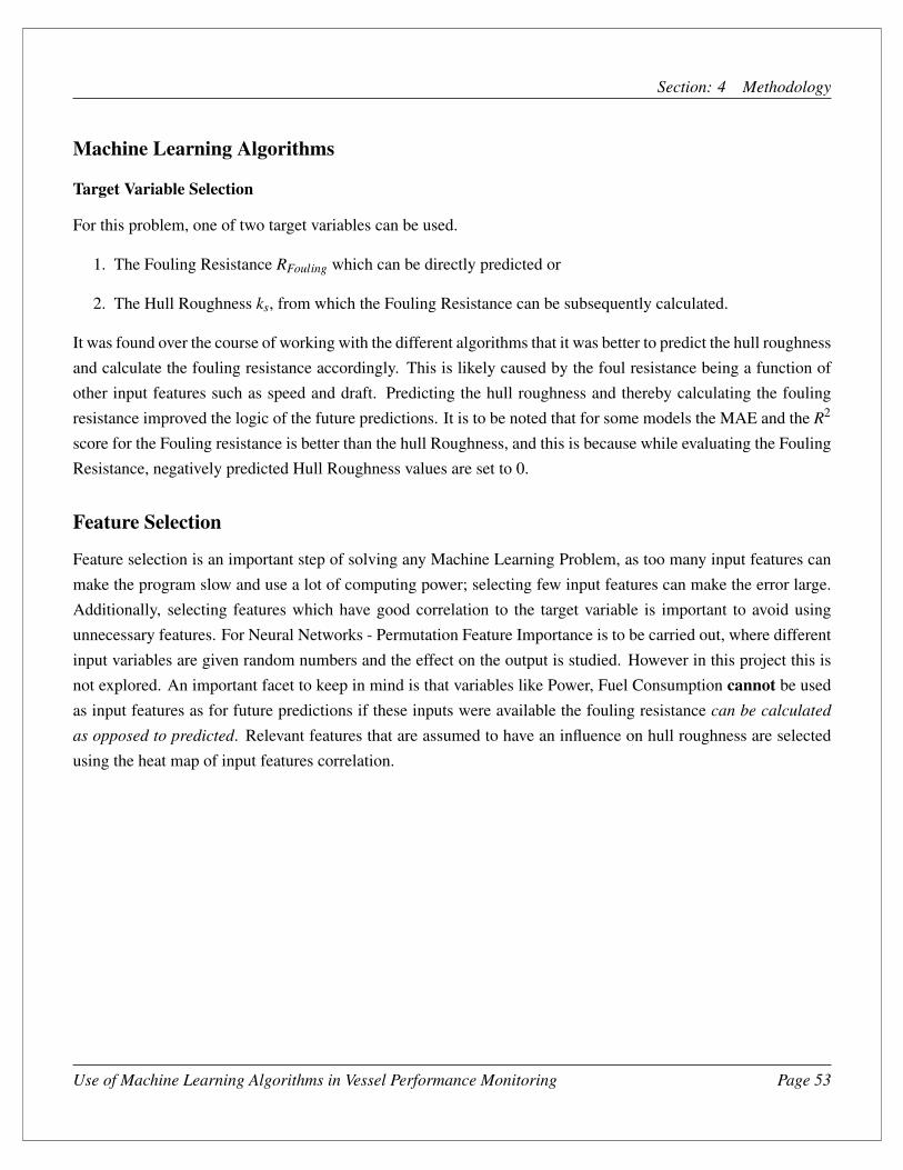
Section: 4 Methodology
Machine Learning Algorithms
Target Variable Selection
For this problem, one of two target variables can be used.
1. The Fouling Resistance RFouling which can be directly predicted or
2. The Hull Roughness ks, from which the Fouling Resistance can be subsequently calculated.
It was found over the course of working with the different algorithms that it was better to predict the hull roughnessand calculate the fouling resistance accordingly. This is likely caused by the foul resistance being a function ofother input features such as speed and draft. Predicting the hull roughness and thereby calculating the foulingresistance improved the logic of the future predictions. It is to be noted that for some models the MAE and the R2
score for the Fouling resistance is better than the hull Roughness, and this is because while evaluating the FoulingResistance, negatively predicted Hull Roughness values are set to 0.
Feature Selection
Feature selection is an important step of solving any Machine Learning Problem, as too many input features canmake the program slow and use a lot of computing power; selecting few input features can make the error large.Additionally, selecting features which have good correlation to the target variable is important to avoid usingunnecessary features. For Neural Networks - Permutation Feature Importance is to be carried out, where differentinput variables are given random numbers and the effect on the output is studied. However in this project this isnot explored. An important facet to keep in mind is that variables like Power, Fuel Consumption cannot be usedas input features as for future predictions if these inputs were available the fouling resistance can be calculated
as opposed to predicted. Relevant features that are assumed to have an influence on hull roughness are selectedusing the heat map of input features correlation.
Use of Machine Learning Algorithms in Vessel Performance Monitoring Page 53

Section: 4 Methodology
KVLCC2
Figure 24: Heat-map showing correlation of various features for KVLCC2
It can be seen that the fouling resistance correlates well with the Vessel Paint Age, The days since the last hullcleaning (Cleaned Days) , the paint CEFF value and the hull roughness, all factors in Malone’s expressionsThe still water resistance, loading condition, propulsive efficiency and other resistances have a low correlation,however they are still used in the algorithm when modelling the data set.
Use of Machine Learning Algorithms in Vessel Performance Monitoring Page 54

Section: 4 Methodology
Vessel 1
Figure 25: Heat-map showing correlation of various features for Vessel 1
Variables like the Event Type (Encoded Event_1,Encoded_Event_2, as mentioned in Tab:3), Days since Last
Cleaning, Days since last Prop Cleaningand MAA Total have comparatively low correlation with the Hull Rough-ness ks - The Paint CEFF Value has a slightly better correlation - however the need for these variables will bedemonstrated in succeeding sections.
Structure of the LSTM Networks Model
The LSTM network is built as explained in the previous sections, with 750 Neurons in the bottom layer with tanh
and a Dense layer with a single unit with a basic Neural network to give a single output. The tanh activation isused, as it is desired that input values of 0 give an activation of 0, as illustrated in the previous section. Afterseveral iterations - the following configuration was seen to work the best with the dataset. The model is optimizedwith the Adam Optimizer, and the MAE loss, and trained with a batch size of 180 days (In the case of the KVLCC2this is 1800 records and in the case of Vessel 1, this is 180 records.) and when training the dataset, the trainingdata set itself is set as the validation dataset. The fit of the LSTM network with Test data can be observed, howeverit is not considered of predominant importance in this project - as much as the logic of future predictions in thecase of different cases. This will be elaborated further in succeeding sections.
Use of Machine Learning Algorithms in Vessel Performance Monitoring Page 55

Section: 4 Methodology
Future Predictions for Vessel 1
In order to evaluate the future predictions of the different algorithms, a random sample of 180 recorded is selectedfrom the available dataset of Vessel 1, and it is assumed this dataset continues from the last record of the totaldataset. It is to be noted that the sequence of this dataset will be slightly erratic (For example, the loading conditioncan switch between loaded and ballast), however this is ignored. For the selected input features, the followingassumptions are made
1. SpeedThe speed is selected from a normal distribution of 1000 numbers, generated from the randomly selectedrecord speed as
UFuture ∼ N(URandom Record,0.0025) (53)
(Or with mean as the randomly selected record’s speed, between extreme values between ±0.5m/s).
2. DraftThe draft is evaluated in the same fashion ;
TFuture ∼ N(TRandom Record,0.0025) (54)
(Or with mean as the selected record’s draft, between extreme values between ±0.5m)
3. Still Water Resistance and Propulsive EfficiencyThe still water resistance and propulsive Efficiency ηProp is then calculated based on the randomised speedand draft values using Holtrop-Mennen Expressions.
4. Wind ResistanceThe wind resistance of the future record is generated from the randomly selected record, by generating anormal distribution of 1000 numbers in the following fashion
RWindFuture ∼ N(RWindRandom Record ,111,111) (55)
(Or with mean value as the wind resistance of the randomly selected record, with extreme values between±1kN. )
5. Added Resistance ResistanceThe added resistance in waves of the future record is generated from the randomly selected record in thesame fashion from a generated normal distribution of 1000 numbers as
RAdded Resistance in WavesFuture ∼ N(RAdded Resistance in WavesRandom Record ,44.44×106) (56)
Use of Machine Learning Algorithms in Vessel Performance Monitoring Page 56

Section: 4 Methodology
(Or with mean value as the wind resistance of the randomly selected record, with extreme values between±20kN. )
In this process, the future predictions are ensured to have different values from the original dataset. Thevalues of Vessel Paint Age, Days since Last Cleaning, Days since Prop Cleaning, Cumulative Port Day areall set to the values based on the last record of the data received. The future predictions of the algorithmsare evaluated in three different cases.
(a) Case 1: No Hull CleaningIn this case, the hull is not cleaned, and the values of ’Vessel Paint Age, Days since Last Cleaning,
Days since Prop Cleaning, Cumulative Port Day’ increment through the 180 records.
(b) Case 2: Hull Cleaned and Propeller Polished on the 90th DayIn this case, it is assumed that the Hull is cleaned after 90 days - therefore the values of the features
’Days since Last Cleaning, Days since Prop Cleaning, Cumulative Port Day’ are reset to 0 at Day 90and then increase. The Vessel Paint Age is not reset.
(c) Case 3: Vessel Dry Docking on the 90th DayIn this case, it is assumed that the vessel is docked after 90 days - therefore the values of ’Vessel Paint
Age, Days since Last Cleaning, Days since Prop Cleaning, Cumulative Port Day’ are all reset to 0at Day 90 and then increase. A single day’s dry docking is not feasible in reality, but for the sake ofevaluating the algorithm’s output predictions it is considered.In all cases mentioned, correspondingly the values of Encoded Event Type are also modified.
6. Anti Fouling Paint Effectiveness Factor CEFFThis parameter is evaluated using Malone’s expressions, and according to the painting scheme in Period 4,this value is mostly 0 as the paint hasn’t failed in this period. After the hull is repainted in Case 3, the paintis assumed to have the same properties as the values in Painting Scheme 4, given in Tab: 7.
7. Total Fouling Roughness MAATotal
This is calculated using Malone’s expressions and the assumptions given in Tab: 7. After the hull is re-painted in Case 3, the paint is assumed to have the same properties as the values in Painting Scheme 4,given in Tab: 7.
Use of Machine Learning Algorithms in Vessel Performance Monitoring Page 57

Section: 5 Results
5 Results
KVLCC2
Linear Regression
Linear Regression using the Ordinary Least Squares method as explained in the previous sections is carried out.While fitting the data, the Mean Absolute Error and R2 is evaluated based on the complete respective data setgiven to the model. The following are the input features used model the data.
Input Features - KVLCC2Data Used Unit
Speed [m/s]Loading ConditionStill Water Resistance [N]Propulsive EfficiencyWind Resistance [N]Vessel Paint Age in Days [days]Cleaned Days [days]Cumulative Port days [days]CEFF ValueTarget: Surface Roughness [µm]
Table 8: Input Features for Linear Regression Model - KVLCC2
From the following plot - it can be seen that linear regression does not give a very good fit to the input data, ratherit predicts a slight increase in hull roughness till the hull is cleaned (as per given inputs this is every 240 days).
Use of Machine Learning Algorithms in Vessel Performance Monitoring Page 58

Section: 5 Results
Figure 26: Linear Regression - Plot of Model Predictions vs Target Variable, KVLCC2
Though the plot for the data shows a relatively poor fit, the MAE and R2 score of linear regression are good.
OLS Model - Fit and Error MAE R2
Surface Roughness [µm] 6.50 0.59Fouling Resistance [kN] 2.27 0.60
Table 9: Linear Regression - MAE and R2 Values, KVLCC2
Use of Machine Learning Algorithms in Vessel Performance Monitoring Page 59

Section: 5 Results
LSTM
In order to first train the LSTM Network - it was first set up with the total dataset - however as it consisted of25000 data points, it took a considerable amount of time to compute. As it was of import to model the data afterthe paint failed, it was considered to model the data in the time between when the hull paint fails (Year 3) andwhen the hull is repainted (Year 5). After removing the rest of the data points - the model was trained using 80%of the data and tested on the remaining data. As it can be observed - the LSTM network does gives a much betterfit to the data, and though it doesn’t not match with the test data exactly - it still does give reasonable predictions.
Figure 27: LSTM - Plot of Model Predictions vs Target Variable, KVLCC2
It can be observed that the LSTM still has MAE and R2 values comparable to that of the Linear Regression Model,but it is to be kept in mind that if the MAE and R2 for the Linear Regression model were calculated only for thedata points between Year 3-5, the error value would be greater and the fit would be poorer. It can be seen that theLSTM model is able to model Malone’s expressions better than the Linear Regression model.
LSTM - Fit and Error MAE R2
Surface Roughness [µm] 6.66 0.61Fouling Resistance [kN] 2.38 0.62
Table 10: LSTM - MAE and R2 Values, KVLCC2
Use of Machine Learning Algorithms in Vessel Performance Monitoring Page 60

Section: 5 Results
Vessel 1
Linear Regression
Linear Regression using OLS as explained in the preceding sections is carried out. While fitting the data, theMean Absolute Error and R2 is evaluated based on the complete respective data set given to the model, and forthis reason, it is not necessary to split the data into training and testing data sets for linear regression. Addingdifferent input features at different stages, the MAE, R2 and logic of the predicted fouling resistance is studied.
1st Model - Using only the available features
Using the following features, different models are generated using different segments of the input data, and theiraccuracy and R2 value are observed.
Input Features for Vessel 1 - 1st ModelData Used Unit
Encoded Report TypeEncoded Cleaning EventSpeed [m/s]Encoded Loading ConditionDraft [m]Still Water Resistance [N]Propulsive EfficiencyWind Resistance [N]Added Resistance in Waves [N]Target: Surface Roughness [µm]
Table 11: Inputs for the 1st OLS Model Type
Two types of models are considered - one where the a single linear regression model is generated based on thecomplete dataset termed Universal Model, and one where individual models are created for the different periodsbetween the dry docking, termed Separated Models
Use of Machine Learning Algorithms in Vessel Performance Monitoring Page 61
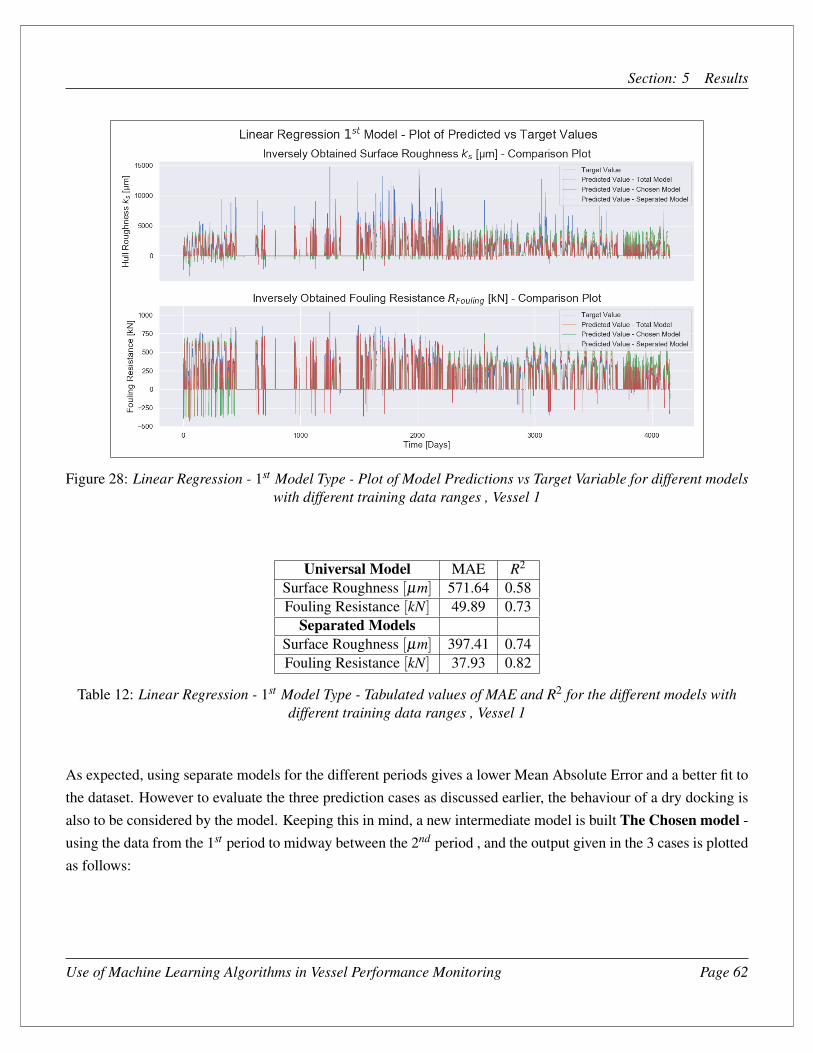
Section: 5 Results
Figure 28: Linear Regression - 1st Model Type - Plot of Model Predictions vs Target Variable for different modelswith different training data ranges , Vessel 1
Universal Model MAE R2
Surface Roughness [µm] 571.64 0.58Fouling Resistance [kN] 49.89 0.73
Separated ModelsSurface Roughness [µm] 397.41 0.74Fouling Resistance [kN] 37.93 0.82
Table 12: Linear Regression - 1st Model Type - Tabulated values of MAE and R2 for the different models withdifferent training data ranges , Vessel 1
As expected, using separate models for the different periods gives a lower Mean Absolute Error and a better fit tothe dataset. However to evaluate the three prediction cases as discussed earlier, the behaviour of a dry docking isalso to be considered by the model. Keeping this in mind, a new intermediate model is built The Chosen model -using the data from the 1st period to midway between the 2nd period , and the output given in the 3 cases is plottedas follows:
Use of Machine Learning Algorithms in Vessel Performance Monitoring Page 62

Section: 5 Results
Figure 29: Linear Regression - 1st Model Type - Future Predictions for the Three Cases(Model built fromSelected Range)
It can be observed this model does not predict any changes in hull roughness and thereby fouling resistance in thethree cases, as there is only one feature that changes between the three cases, the "Event Type" (Encoded EventType). Therefore though this model has a good fit and reasonable errors values, this model can not be used topredict any fouling resistance improvements in the case of hull cleaning or repainting.
Use of Machine Learning Algorithms in Vessel Performance Monitoring Page 63

Section: 5 Results
2nd Model - Adding the Day Counter features to improve Predictability
In order to improve the future predictions of the model, the variables ’Vessel Paint Age, Days since Last Cleaning,
Days since Prop Cleaning, Cumulative Port Day’ are added to the input features as mentioned previously, and thesame process is repeated. It is to be kept in mind that from the Heat-map that these parameters have comparativelylow correlation with the hull roughness parameter and the fouling resistance as well.
Figure 30: Linear Regression - 2nd Model Type - Plot of Model Predictions vs Target Variable for differentmodels with different training data ranges , Vessel 1
Note that the chosen model is built on data from Period 1 to midway between Period 2, and because of this - thismodel predicts extremely high values in Period 0, as the values of the different Day counter parameters in thisperiod are higher than those in the rest of the data set.
Use of Machine Learning Algorithms in Vessel Performance Monitoring Page 64
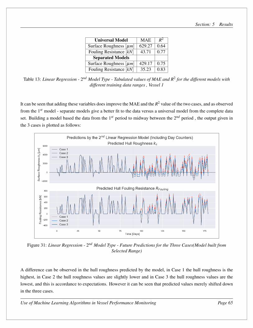
Section: 5 Results
Universal Model MAE R2
Surface Roughness [µm] 629.27 0.64Fouling Resistance [kN] 43.71 0.77
Separated ModelsSurface Roughness [µm] 429.17 0.75Fouling Resistance [kN] 35.23 0.83
Table 13: Linear Regression - 2nd Model Type - Tabulated values of MAE and R2 for the different models withdifferent training data ranges , Vessel 1
It can be seen that adding these variables does improve the MAE and the R2 value of the two cases, and as observedfrom the 1st model - separate models give a better fit to the data versus a universal model from the complete dataset. Building a model based the data from the 1st period to midway between the 2nd period , the output given inthe 3 cases is plotted as follows:
Figure 31: Linear Regression - 2nd Model Type - Future Predictions for the Three Cases(Model built fromSelected Range)
A difference can be observed in the hull roughness predicted by the model, in Case 1 the hull roughness is thehighest, in Case 2 the hull roughness values are slightly lower and in Case 3 the hull roughness values are thelowest, and this is accordance to expectations. However it can be seen that predicted values merely shifted downin the three cases.
Use of Machine Learning Algorithms in Vessel Performance Monitoring Page 65

Section: 5 Results
3rd Adding features from Malone’s Expressions to improve the Results
For the final model, two parameters from Malone’s expressions - MAATotal and CEFF are added to the abovemodel, and then again the fit of the model with the data is studied.
Figure 32: Linear Regression - 3rd Model Type - Plot of Model Predictions vs Target Variable for differentmodels with different training data ranges , Vessel 1
Again it is to be noted that the chosen model is built on data from Period 1 to midway between Period 2, andbecause of this - this model predicts extremely high values in Period 0, as the values of the Day counter parametersin this period are higher than those in the rest of the data set. Adding these parameters does not improve the MAEor the R2, but a appreciable difference can be seen in the future predictions of this model, as can be seen in thefollowing plot.
Use of Machine Learning Algorithms in Vessel Performance Monitoring Page 66

Section: 5 Results
Universal Model MAE R2
Surface Roughness [µm] 628.15 0.64Fouling Resistance [kN] 44.16 0.77
Separated ModelsSurface Roughness [µm] 428.63 0.75Fouling Resistance [kN] 35.13 0.84
Table 14: Linear Regression - 3rd Model Type - Tabulated values of MAE and R2 for the different models withdifferent training data ranges , Vessel 1
Figure 33: Linear Regression - 3rd Model Type - Future Predictions for the Three Cases(Model built fromSelected Range)
A clear improvement can be observed between the three cases, though the model still predicts negative hull rough-ness values. Therefore adding these parameters does improve the model, even though it does not improve the fitof the model itself greatly.
Use of Machine Learning Algorithms in Vessel Performance Monitoring Page 67

Section: 5 Results
The choice of the ’Chosen Model’ Data range
As seen, the chosen model which uses only the data from Period 1 to midway between period 2 is used to givepredictions, as opposed to other possible period combinations. The reason why this particular range is chosen is -as observed earlier this is the range where the data follows expectations (i.e. hull cleaning improves the roughnessetc). However, this period range also observes relatively higher fouling resistance values, which can be observedin the predicted values - where the predictions are all among the range of 600 kN and higher - quite high valuesof fouling resistance. Let us consider the predictions based on a model based on the total dataset.
Figure 34: Linear Regression - 3rd Model Type - Future Predictions for the Three Cases(Model built from TotalDataset)
Here something interesting can be observed - where in the case of the hull being cleaned the hull roughness ispredicted to be higher than when it is not cleaned. A prediction that is contrary to expectations, but still in line withthe majority of the observed data. The applicability of this prediction needs to be studied further. Additionally thefouling resistance values predicted are still on the higher end. Let’s consider a model made from the data fromPeriod 2-4.
Use of Machine Learning Algorithms in Vessel Performance Monitoring Page 68

Section: 5 Results
Figure 35: Linear Regression - 3rd Model Type - Future Predictions for the Three Cases(Model built from Datafrom Period 2-4)
The same pattern can be observed, though the overall resistance values given are more aligned to the recentlyobserved resistance values. In order to build a model which can make predictions which follow the expectedvalues, the range of data between Period 1 to midway between Period 2 is considered.For all the models, it can be observed that not all of them are able to capture the sudden ’spikes’ in the hullroughness (except for some extent the separated models), and this is to be expected as these spikes themselves arequite random.
Drawbacks
1. As it can be observed, the predictions do not necessarily predict a trend but rather just a downward shift inthe roughness/resistance values.
2. The model does predict negative hull roughness values, which is not desirable.
In order to overcome the above drawbacks, and the variation in predicted trends based on the input data, LSTMnetworks are considered.
Use of Machine Learning Algorithms in Vessel Performance Monitoring Page 69

Section: 5 Results
LSTM
The LSTM Networks are built with the configuration previously specified. The network is made to train over afew epochs in order to stop the network from overfitting the data, but at the same time it is ensured that the lossvalue does reduce over the iterations. The obtained models are saved and reloaded to make predictions in thedifferent cases, and the input file in the case of the different predictions are modified accordingly as well. Afterevaluating the results from the different models, the MAE and the R2 value of the model over the training data iscalculated. In the following sections, the input dataset is not split into training or testing data, but is given to themodel as a whole to appraise how well the algorithm models the total dataset. Doing this training-test data splitcan reduce the bias of the model (if any) but it is not considered of importance in this paper, as the logic of themodel’s predictions were of more significance.1st Model - Using only the available featuresAn LSTM network is built as explained in the previous sections, using only the inputs given in Tab: 11, to observeif the Algorithm is capable of modelling the data without the day counters.
Figure 36: LSTM - 1st Model Type - Plot of Model Predictions vs Target Variable for model trained with TotalDataset, Vessel 1
It appears that the LSTM model is not able to model the hull roughness without the day counter features, thoughthe calculated fouling resistance do fit considerably well. Therefore this model can model the inversely obtainedfouling resistance well, as seen from the MAE and R2 score of the model.
Use of Machine Learning Algorithms in Vessel Performance Monitoring Page 70
Section: 5 Results
LSTM - Fit and Error - 1st Model MAE R2
Surface Roughness [µm] 480.95 0.50Fouling Resistance [kN] 43.98 0.81
Table 15: LSTM - 1st Model Type - Tabulated Values of MAE and R2 , Vessel 1
When using this model to predict improvements in the hull roughness in the future cases as described earlier, thefollowing output was observed.
Figure 37: LSTM - 1st Model Type - Future Predictions for the Three Cases(Model built from Total Dataset)
It can seen that there is no change in the outputs given by the model, therefore though this model can to an extentpredict the future fouling resistances, it can not predict an improvement in resistances in the event of a hull clean-ing or hull repainting event, though the predicted fouling resistances are on the higher side.
Use of Machine Learning Algorithms in Vessel Performance Monitoring Page 71

Section: 5 Results
2nd Model - Adding the Day Counter Features
In the next step, an LSTM model is built by adding the day counter features such as the ’Vessel Paint Age,
Days since Last Cleaning, Days since Prop Cleaning, Cumulative Port Day’ to the features mentioned in Tab: 11,and the following plot was observed.
Figure 38: LSTM - 2nd Model Type - Plot of Model Predictions vs Target Variable for model trained with TotalDataset, Vessel 1
This model clearly gives a superior fit to the hull roughness data than the previous model. Let’s consider two moremodels, one built with the data from Period 2 to Period 4, and another built with the data from Period 3 to Period4.
Use of Machine Learning Algorithms in Vessel Performance Monitoring Page 72

Section: 5 Results
Figure 39: LSTM - 2nd Model Type - Plot of Model Predictions vs Target Variable for model trained with Datafrom Period 2-4, Vessel 1
Figure 40: LSTM - 2nd Model Type - Plot of Model Predictions vs Target Variable for model trained with Datafrom Period 3-4, Vessel 1
Use of Machine Learning Algorithms in Vessel Performance Monitoring Page 73

Section: 5 Results
It can be easily observed that these models fit the data from their relevant periods better than the the rest of thedata set, and this can also be observed in the case of the MAE and R2 values as well.
LSTM - Fit and Error - 2st Model MAE R2
Universal ModelSurface Roughness [µm] 421.74 0.64Fouling Resistance [kN] 39.26 0.85
From Period 2-4Surface Roughness [µm] 478.66 0.60Fouling Resistance [kN] 43.52 0.74
From Period 3-4Surface Roughness [µm] 587.15 0.32Fouling Resistance [kN] 64.31 0.47
Table 16: LSTM - 2nd Model Type - Tabulated Values of MAE and R2 , Vessel 1 for the different Models trainedwith different data sets
Note: When evaluating the error and R2 for the Models From Period 2-4 and the model Model 3-4, the data from Period
0 is removed, as the data in this period has high values in comparison to the rest of the dataset, thereby giving inaccurate
error and fit values.
Now to evaluate the future predictions from these generated models.
Figure 41: LSTM - 2nd Model Type - Future Predictions for the Three Cases(Model built from Total Dataset)
Use of Machine Learning Algorithms in Vessel Performance Monitoring Page 74

Section: 5 Results
In the case of the model built from the total dataset, the same difficulty as before arises, where the model predictsa better hull roughness when the hull is not cleaned as opposed to cleaned, which is contrary to expectations. Forthe second model based on data from Period 2 - 4 , this same issue can be observed.
Figure 42: LSTM - 2nd Model Type - Future Predictions for the Three Cases(Model built from Data from Period2-4)
For the predictions from the model built with the data from Period 3-4, the predictions are in accordance toexpectations, however the model predicts almost marginal improvements for the different cases, as the inputtraining data has no individual hull cleaning events, except for during the vessel dry docking. The values of theresistance itself are more in-line with the fouling resistance values observed in Period 4 - of the range 400 -600kN.
Use of Machine Learning Algorithms in Vessel Performance Monitoring Page 75

Section: 5 Results
Figure 43: LSTM - 2nd Model Type - Future Predictions for the Three Cases(Model built from Data from Period3-4)
Use of Machine Learning Algorithms in Vessel Performance Monitoring Page 76

Section: 5 Results
3rd Model - Adding the features from Malone’s ExpressionsA final model is considered, with both the days counter features and adding two features from Malone’s expres-sions - the MAATotal calculated, and the Anti fouling paint effectiveness factor CEFF .
Figure 44: LSTM - 3rd Model Type - Plot of Model Predictions vs Target Variable for model trained with TotalDataset, Vessel 1
The overall fit of the data with the target values does improve. Let us consider the 2 models in the same fashionseen earlier - one trained with the data from Period 2-4 and another trained with data from Period 3-4.
Use of Machine Learning Algorithms in Vessel Performance Monitoring Page 77

Section: 5 Results
Figure 45: LSTM - 3rd Model Type - Plot of Model Predictions vs Target Variable for model trained with Datafrom Period 2-4, Vessel 1
Figure 46: LSTM - 3rd Model Type - Plot of Model Predictions vs Target Variable for model trained with Datafrom Period 3-4, Vessel 1
Use of Machine Learning Algorithms in Vessel Performance Monitoring Page 78

Section: 5 Results
LSTM - Fit and Error - 3st Model MAE R2
Universal ModelSurface Roughness [µm] 374.95 0.70Fouling Resistance [kN] 35.01 0.87
From Period 2-4Surface Roughness [µm] 409.53 0.65Fouling Resistance [kN] 36.34 0.82
From Period 3-4Surface Roughness [µm] 445.66 0.54Fouling Resistance [kN] 38.59 0.81
Table 17: LSTM - 3rd Model Type - Tabulated Values of MAE and R2 , Vessel 1 for the different Models trainedwith different data sets
Note: When evaluating the error and R2 for the Models From Period 2-4 and the model Model 3-4, the data from Period
0 is removed, as the data in this period has high values in comparison to the rest of the dataset, thereby giving inaccurate
error and fit values.
As it can be seen from the MAE and the R2 values, these models do provide a slightly improved fit than theprevious case, and as observed earlier - these models fit the input data better in their relevant data ranges than therest of the dataset. Now the future predictions from the different models are considered.
Figure 47: LSTM - 3rd Model Type - Future Predictions for the Three Cases(Model built from Total Dataset)
Use of Machine Learning Algorithms in Vessel Performance Monitoring Page 79
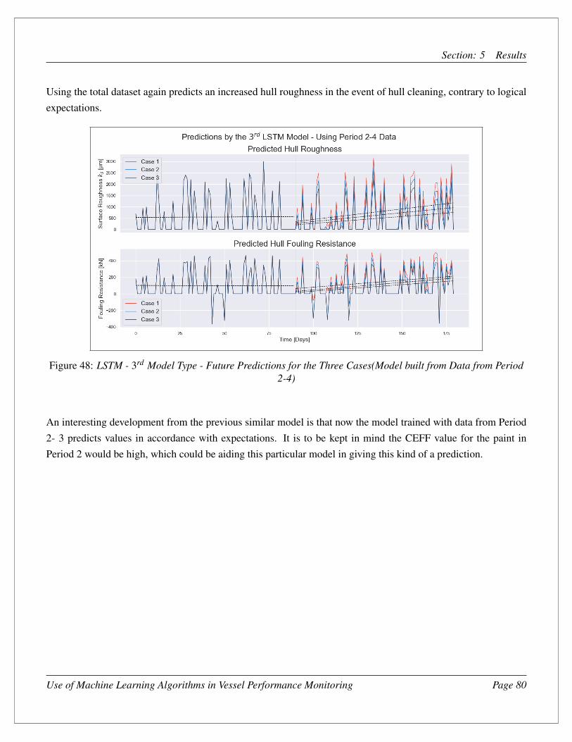
Section: 5 Results
Using the total dataset again predicts an increased hull roughness in the event of hull cleaning, contrary to logicalexpectations.
Figure 48: LSTM - 3rd Model Type - Future Predictions for the Three Cases(Model built from Data from Period2-4)
An interesting development from the previous similar model is that now the model trained with data from Period2- 3 predicts values in accordance with expectations. It is to be kept in mind the CEFF value for the paint inPeriod 2 would be high, which could be aiding this particular model in giving this kind of a prediction.
Use of Machine Learning Algorithms in Vessel Performance Monitoring Page 80
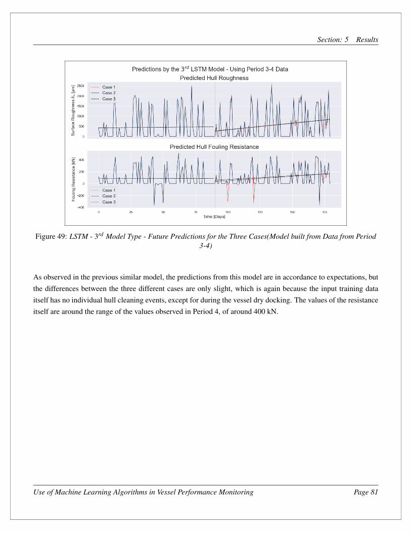
Section: 5 Results
Figure 49: LSTM - 3rd Model Type - Future Predictions for the Three Cases(Model built from Data from Period3-4)
As observed in the previous similar model, the predictions from this model are in accordance to expectations, butthe differences between the three different cases are only slight, which is again because the input training dataitself has no individual hull cleaning events, except for during the vessel dry docking. The values of the resistanceitself are around the range of the values observed in Period 4, of around 400 kN.
Use of Machine Learning Algorithms in Vessel Performance Monitoring Page 81

Section: 5 Results
Malone’s Predictions
Finally, as the various parameters to use Malone’s Expressions are already inversely arrived at, the hull foulingresistance given by Malone’s expressions are calculated.
Figure 50: Malone’s Expressions - Future Predictions for the Three Cases
As it can be seen, Malone’s expressions do not give any improvement in the fouling resistance, though the hullroughness improves when the hull is repainted. This is because it is considered that the hull is repainted before itfails, therefore the only improvement is the roughness due to the MAACoating, which is marginal. No improvementis observed when the hull is cleaned, because as the hull paint hasn’t failed there is no fouling observed, bothbefore and after the hull cleaning. The values of the resistance are quite high compared to the resistance valuesobserved in Period 4.
Use of Machine Learning Algorithms in Vessel Performance Monitoring Page 82

Section: 6 Inferences
6 Inferences
The Data
Keeping in mind the assumptions made, the differences in the fouling resistance given by Malone’s expressionsfor fouling resistance the KVLCC2 and the observed fouling resistance in Vessel 1 are significant. As it can beseen that Malone’s expressions reflect a simplistic nature of hull fouling, where hull fouling does not occur atall till the hull anti fouling paint fails, and even after the paint fails - it still does not loose its total effectivenessimmediately and repainting the hull returns the hull to its new ship condition. Working with the data from Vessel 1,it can be seen that this is not the case - the hull does experience additional resistances even after being repainted -which in this project is considered to be the fouling resistance. The hull roughness can be observed to be low afterthe vessel is repainted, but the baseline roughness is never as low as the new hull, presumably due to sandblastingthe underwater hull. Therefore it can be concluded that the hull roughness in reality and consequently the foulingresistance are far from Malone’s idealistic expressions. This is not to say Malone’s expressions can be disregardedas it has been shown that the various parameters from Malone’s expression can be added to available features toimprove modelling of the fouling resistance.
The use of ITTC-78 vs Holtrop & Mennen Expressions
As seen in the Methodology section, when using equations from Holtrop & Mennon3 to evaluate the still waterresistance and calculating the Inversely calculated fouling resistance , it can be seen that often the inverselycalculated fouling resistance is found to be negative. It can be argued that Holtrop & Mennon’s expressions give aconservative value of still water resistance, in comparison to other methods of evaluating the still water resistancesuch as Guldhammer and Harvald or Hollenbach. Understandably the value of the Inversely Calculated FoulingResistance and consequently the Inversely calculated hull roughness will be different when using the differentmethods, the value of the inversely calculated hull roughness obtained must be investigated before proceedingwith the results, because as shown - hull roughness can not take a negative value. In the expressions for the foulingresistance coefficient used in this paper (given by Holtrop & Mennen) the equation does not consider the vesselspeed. ITTC-78’s expressions do consider the vessel speed in the evaluation of the fouling resistance coefficient(in the form of the Reynold’s number) and the inter-relatedness between these two features can additionallyadd another level of understanding the nature of vessel hull fouling. However as discussed - negative foulingresistances can be observed in both cases - but in the case of the ITTC -78 expressions (refer Fig: 17), at lowerspeeds - substantially higher hull roughness values can still give a negative fouling resistance coefficient, whichis to be kept in mind if this method is used. It can be considered that the ITTC-78’s expressions are better suitedfor evaluating the vessel resistance during the vessel design stages, and the use of these expressions to evaluaterecorded data to study hull fouling resistances values is to be done with care.
Use of Machine Learning Algorithms in Vessel Performance Monitoring Page 83
Section: 6 Inferences
The Fouling Resistance
In the case of the KVLCC2, it is given by Malone’s expressions, and for a 320m ship is calculated to be of therange of only 30kN. In the case of Vessel 1, it can be seen that the observed values of fouling resistance are inthe range of 200-600kN, with occasionally spikes to higher numbers as well. With Vessel 1, where it is inverselycalculated using the vessel’s fuel consumption, it can seen that the long term data is contrary to expectationsin some areas. There are periods where a hull cleaning shows an increase in the trend of fouling resistance,there are periods where the trend line of the fouling resistance is decreasing as opposed to increasing. Thesediscrepancies can be seen to be absorbed by the model as well, as shown in the previous section. Keeping in mindthe assumptions made - the recorded data does appear to sometimes defy expectations. This is to be kept in mindwhile choosing the model and its training data, and it can be observed that sometimes using the total dataset iserroneous.It is to be noted that the Wake Fraction and the Thrust deduction factor for Vessel 1 has a few irregularities -where the wake fraction at specific drafts differs greatly from the nearby values, specifically around 11.1m. Thisdiscrepancy could give rise to some irregular values in the propulsive efficiency ηProp values.On average, the fouling resistance makes up approximately 10% of the total resistance in the case of Vessel 1, andit is understood and that any procedures that can result in the improvements of this number can lead to significantreduction in vessel fuel consumption.
The Effectiveness of Hull Cleaning
Based on the dataset from Vessel 1, it would be specious to conclude that Hull cleaning does not contribute toimprovements in the fouling resistance. The data at different time periods differs in operating area and profile,as well as several other factors. It can also be argued that the fouling resistance could have been worse were thehull not cleaned. In the same fashion that no two hulls can have the exact same hull fouling, no two hull cleaningevents can be said to have the same effect because of these intricate differences. In order to truly evaluate theeffectiveness of hull cleaning, it would be required to study vessels with the same operating profile and operatingarea between the same type of vessel, or evaluate several datasets from different vessels, and normalize the datato a common value based on different reasonable assumptions.
Use of Machine Learning Algorithms in Vessel Performance Monitoring Page 84

Section: 6 Inferences
The Machine Learning Algorithms
KVLCC2
For the KVLCC2, the dataset is quite simplified and the Machine Learning algorithms are able to essentiallymodel Malone’s expressions relatively well. It can be seen that the LSTM model is much better than the LinearRegression model, though the latter can be improved on if more input features are considered.
Vessel 1
It can be observed that Machine Learning Algorithms can model the Fouling resistance observed by the hull.Linear Regression can give a quick and simple model of the fouling resistance, and using features from Malone’sexpressions helps improve the model quite well.
The LSTM network shows marked improvements over the Linear Regression, in that the model uses thememory of the hull roughness (and consequently the fouling resistance) in the last period of the data set andpredicts values in accordance to the recent data, something the linear regression model can not do. However it canbe seen that the choice of the input features and the training data range of the model affects the outputs markedly.
Linear Regression vs LSTM Models
It can be observed that the Linear Regression models’ prediction are more of a shift in the values as opposed to apredicted trend. Considering the results from the most suitable Linear Model and LSTM Networks for Vessel 1,the following can be seen:
Use of Machine Learning Algorithms in Vessel Performance Monitoring Page 85

Section: 6 Inferences
Figure 51: Most suitable Linear Regression vs LSTM Model - Future Prediction Comparison
Linear regression gives predictions along the same range as its training data (between Period 1- to midway be-tween Period 2.) where the resistance values are one the higher side. Consequently this model predicts foulingresistances around 600-800 kN, which is higher than the values seen in Period 4. The improvement itself predictedby the different cases is of the order of about 100kN between each of the three cases, at its peak value. The LSTMmodel predicts resistances in the range of 200-400kN - as it has modelled the patterns overall and the therebypredicts roughness and thereby resistance values in a more expected range, based on more recent values. Theimprovement itself predicted by the different cases is of the order of about 50kN between each of the three cases,at its peak value. The author strongly feels that the LSTM network’s predictions are more in line with expectedvalues of fouling resistance.
Use of Machine Learning Algorithms in Vessel Performance Monitoring Page 86

Section: 6 Inferences
The Anti Fouling Paint Effectiveness Factor, CEFF
In the case of the KVLCC2, the effect of this factor can be clearly seen - there is no hull growth up unto the pointthe hull anti fouling paint fails at 3 years, and after the paints - the paint still contributes marginally to preventinghull growth till the hull is repainted at 5 years. However in the case of Vessel 1, where the values of the EffectivePaint Life had to be assumed in order to match the observed fouling resistance - it can be seen that the value ofthe Effective Paint Life is quite low. Compared to the paint Product Data sheet values of product life of 7.5 years(JOTUN, 2018)17 - it can be seen that the inversely arrived-at values are comparative low. It is understood thatthe product data sheet value refers to the overall lifetime of the paint considering several other factors ; howeversimilar factor such as the CEFF can be included by paint company manufacturers for different paints - whichconsiders the time period over which the hull anti fouling paint is most effective.
PaintingScheme
for differentPeriods
Anti Fouling PaintEffective Life
(Assumed)Years
0 31 1.52 0.53 24 2
Table 18: Values of Effective Paint Life assumed for Vessel 1, in order for Malone’s Expression to yield foulingresistance values to the same extent as the inversely calculated fouling resistance
The Training -Testing Data split
The conventional training-testing data split is not dealt with in detail in this project. An aim of the project wasto consider if the machine algorithms were capable of modelling the input data as a whole, as well as give goodpredictions. For example, consider this case where the model is trained with 80% of the dataset and tested on theremaining 20% of the dataset, a typical train-test process. The model predictions on the test data are observed asfollows:
Use of Machine Learning Algorithms in Vessel Performance Monitoring Page 87

Section: 6 Inferences
Figure 52: LSTM - 3rd Model Type - Plot of Model Predictions vs Target Variable for model trained 80% of theDataset and tested on the remaining 20%
The model does work well - except for predicting the random spikes, however when using this model to makefuture predictions the same discrepancy was observed, where the predictions when the hull is cleaned is greaterthan when the hull is not cleaned. In order to evaluate the logic of the model rather than overall fit with unseentest data, the training -testing data split was not considered it this project, as considering this would only result inmarginal changes in the overall model.
The different input feature combinations
As it has been demonstrated, the models can effectively model the observed fouling resistance - even without theDay counter variables, and adding more features which have little correlation with the hull roughness numerically- has been shown to improve the logic and the practicality of the model’s predictions.
Choosing a suitable Model
It can be observed in some cases that selecting a model which has a low R2 value and high MAE over the entiredataset gives more reasonable results than models which have better R2 values and lower errors. This suggeststhat a model should not be assessed purely on these metrics alone- but also by the practicality of its resultsas well. As the long term recorded data sometimes is contrary to expectations, the decision to chose a modelthat makes expected predictions in accordance with expectations versus a model that gives predictions based on
Use of Machine Learning Algorithms in Vessel Performance Monitoring Page 88

Section: 6 Inferences
observed discrepancies is a decision that is to be made. As it can be seen - the algorithms are capable of modellingboth cases, and choosing an appropriate model is the next step. Adding relevant features, particularly ones thatreflect the paint functionality would be extremely valuable in making the models more balanced = as observed. Asingle dataset can be used to generate several models - using different combinations of input features and trainingdatasets, therefore it can be stated that the next step would involving choosing a suitable model - one that capturesboth the nuances of the observed dataset as well as logical expectations.
Future Improvements
The following are various improvements that can be done in order to obtain better understand of hull fouling.
1. Include the Effects of Shallow Water, Trim, Steering Resistances in the total resistance estimationThough these resistance values are neglected in this project, including these features can improve the datasetand consequently the model - as some of the spikes observed could be attributed to these effects.
2. Split the datasets in the different periods as Training and Test DataSplitting the dataset into training and test data can improve the uncertainty of the model, or remove anyimplicit bias the model develops when being trained, however as stated previously it is expected that thiswill result in marginal changes.
3. Permutation Feature ImportanceAs mentioned earlier, this is a method of calculating the feature importance of a neural network - carry-ing this out on the various possible input features can help in identifying features that though have lowcorrelation with the target variable - aid in building a better model.
4. Isolating the effect of propeller cleaning if possible data sets are availableIt can be argued that a propeller polish can in some cases provide better improvements in hull resistance atcertain times as opposed to a complete hull cleaning, and in order to evaluate this - datasets where the hullalone is cleaned without a propeller polish and then where the propeller is polished without the hull beingcleaned can be studied. The latter would be more easily attainable than the former - but studying datasetscan help study the improvements due to these activities individually.
5. Evaluating the Hull Still Water resistance by different methodsAs it was observed using Holtrop and Mennon’s expressions results in Inversely calculated fouling resis-tances values to be negative for a significant number of the data records. However using different methodsto evaluate the Still Water Resistance such as Guldhammer and Harvald, or Hollenbach could give rise todifferent values of Still Water Resistance, and thereby Inversely Calculated Fouling Resistance.
Use of Machine Learning Algorithms in Vessel Performance Monitoring Page 89

Section: 6 Inferences
6. Use Different Machine Learning AlgorithmsThere are several other kind of machine learning algorithms available - and regression models such asGaussian Process Regression can be considered.
7. Using the LSTM Network with Different Time StepsGenerating different models using different time steps of the training data set can generate Networks whichgive different outputs, and this can also be studied further.
8. Using Features from other Methods to Evaluate the Fouling Resistance As it has been observed, addingfeatures from Malone’s expressions improve the model, this can be further extended to using features fromother methods to calculate the Fouling Resistance.
Use of Machine Learning Algorithms in Vessel Performance Monitoring Page 90

Section: 7 Conclusion
7 Conclusion
Hull fouling is expected to play a part in vessel performance until environment-friendly and effective anti-foulingpaints are developed. Hull fouling will play a factor in all vessels’ performances - be it wind-assisted, battery-operated, biofuel or conventional fuel ships. There is a considerable potential for improving vessel performanceif hull fouling can be determined at different points in time. The ultimate objective of this endeavour would be topinpoint the exact future time at which the cost of the additional fuel consumption due to increased hull foulingwould exceed the cost of cleaning the hull. With increasingly stringent emission regulations and focus on dataanalysis by the International Maritime Organization - evaluating hull fouling and the fouling resistance is an un-dertaking where even a little clarity can bring about sizeable benefits.
Hull fouling can be considered a function of the vessel operating profile, the hull paint and its properties and time -and using these parameters to generate models from existent vessel data can improve the understanding of the hullfouling process. As it has been illustrated, few alterations need to be made to the expressions while evaluating thedata records of vessels, as well as a critical study of the dataset. Several models can be built from a single datasetas demonstrated, based on different combinations of input features and training datasets; and studying carefullywhich model best fits the future data is the next step.
Generating models from the data recorded from different vessels with different operating profiles could help indeveloping empirical relations that can predict the fouling resistance over time, with a given level of accuracy, asafter all hull fouling is still a random process. Models that fit the data well can be used for this purpose, and otherparameters which are expected to influence the hull fouling can be included as well. However, care is to be takenwhile generating these models as the model will reflect its training data. Reducing the level of uncertainty in itsinput data will improve the model immensely. The results from these algorithms can be compared with the vesselfuel consumption in real time and corrected, improved and validated.
The requirement for parameters like ’Effective Paint Life’ and ’Hull Cleaning Effectiveness’ is also evident, asthese attributes can both improve modelling of vessel fouling, as well as give a better comparison and benchmarkthe different aspects of hull paints and underwater hull cleaning.
Hull fouling and fouling resistance can no longer be considered to be a completely random variable, but can bemodelled to a certain degree of accuracy - even individually for different vessels based on its own recorded data,with improvements to the procedures mentioned in this paper and further investigation.
Use of Machine Learning Algorithms in Vessel Performance Monitoring Page 91

Section: References
References1 Malone, J. A., Little, D. E., & Allman, M. Effects of Hull Foulants and Cleaning/Coating on Ship Perfomance
and Economics. SNAME, 88(88).
2 International Towing Tank Conference, (1978). ITTC 1978 Performance Prediction Method 7.5-02 03-01.4,https://www.ittc.info/media/8017/75-02-03-014.pdf
3 Holtrop, J., & ; Mennen, G. (1982). An approximate power prediction method. International ShipbuildingProgress, 166-170. doi:10.3233/isp-1982-2933501
4 IMO. (2018,March). Data Collection System. Retrieved July 11, 2020, fromhttp://www.imo.org/en/OurWork/Environment/PollutionPrevention/AirPollution/Pages/Data-Collection-System.aspx
5 MAN Energy Solutions. (2018, October). Basics of Ship Propulsion. Author. Retrieved fromhttps://marine.man-es.com/docs/librariesprovider6/test/5510-0004-04_18-1021-basic-principles-of-ship-propulsion_web_links.pdf?sfvrsn=12a35ba2_30
6 Géron, A. (2017). Hands-On Machine Learning with Scikit-Learn and TensorFlow: Concepts, Tools, and Tech-niques to Build Intelligent Systems (1st ed.). CA, United States of America: O’Reilly Media.
7 Machine Learning Mastery. (2017b, August 14). Multivariate Time Series Forecasting with LSTMs in Keras. Re-trieved March 27, 2020, from https://machinelearningmastery.com/multivariate-time-series-forecasting-lstms-keras/
8 Anagnostopoulos, A. (2017). Big Data Techniques for Ship Performance study. Gothenburg, Sweden: ChalmersUniversity of Technology.
9 Pedersen, B. P. (2014). Data-driven Vessel Performance Monitoring. Lyngby, Denmark: Technical University ofDenmark.
10 Helland, M. D. (2018, July). Ship technical and economic performance as function of hull cleaning and coatingpractices. Lyngby, Denmark: Technical University of Denmark.
11 Jochen Brix, (1987) Manoeuvring Technical Manual.
12 Poul Anderson (2019), Lecture Notes. Ship Propulsion and Manoeuvring.
13 Martin Alexandersson. (2009, January). A study of methods to predict added resistance inwaves. KTH Centre for Naval Architecture. Retrieved from https://www.kth.se/polopoly_fs/1.151543.1550158721!/Menu/general/column-content/attachment/Alexandersson.pdf
Use of Machine Learning Algorithms in Vessel Performance Monitoring Page 92

Section: References
14 H. B. Bingham (2019), Lecture Notes. Wave Loads on Ships and Offshore Structures
15 DTU Ship Simulation Workbench. (2020). Calculate added resistance RAO using DTU method. Retrieved2020, from https://www.ssw.mek.dtu.dk/dtu_added_resistance
16 Ocean-Wave Spectra. (2012). Retrieved June 07, 2020, from https://wikiwaves.org/Ocean-Wave_Spectra
17 JOTUN. (2018, March). Technical Data Sheet - SeaQuantum Ultra S. Retrieved fromhttps://www.jotun.com/Datasheets/Download?url=%2FTDS%2FTDS__20760__ SeaQuan-tum+Ultra+S__Euk__GB.pdf
18 Townsin, R. L. (2003). The Ship Hull Fouling Penalty. Biofouling, 19(sup1), 9–15.https://doi.org/10.1080/0892701031000088535
19 LITTLE, B. J., & DEPALMA, J. R. (1988). Marine Biofouling. Treatise on Materials Science & Technology,89–119. https://doi.org/10.1016/b978-0-12-341828-9.50009-7
20 Global Maritime Energy Efficiency Partnerships. (n.d.). Hull cleaning. Retrieved July 2, 2020, fromhttps://glomeep.imo.org/technology/hull-cleaning/
21 Bevaldia. (2020, April 14). Underwater Propeller Polishing And Cleaning. Retrieved July 2, 2020, fromhttps://bevaldia.com/underwater-propeller-polishing/
22 Mitutoyo. (1984). Quick Guide to Surface Roughness Measurement. Retrieved fromhttps://www.mitutoyo.com/wp-content/uploads/2012/11/1984_Surf_Roughness_PG.pdf
23 SIMMAN 2008. (n.d.). MOERI KVLCC2, SIMMAN 2008, FORCE Technology. Retrieved July 3, 2020, fromhttp://www.simman2008.dk/KVLCC/KVLCC2/tanker2.html
24 MAN B& W. (2009). MAN B & W. S70MC6 Project Guide Camshaft Controlled Two stroke Engines[Brochure].
25 Molland, A. F. (2008). The Maritime Engineering Reference Book. Butterworth-Heinemann.
26 XLSTAT. (n.d.). Linear Regression. Retrieved June 17, 2020, from https://www.xlstat.com/en/solutions/features/ordinary-least-squares-regression-ols
27 Machine Learning Mastery. (2019, January 30). How to Choose Loss Functions When Training Deep Learn-ing Neural Networks. Retrieved June 17, 2020, from https://machinelearningmastery.com/how-to-choose-loss-functions-when-training-deep-learning-neural-networks/
Use of Machine Learning Algorithms in Vessel Performance Monitoring Page 93

Section: References
28 Towards Data Science. (2019, August 10). Understanding Adam : how loss functions are minimized ? RetrievedJune 17, 2020, from https://towardsdatascience.com/understanding-adam-how-loss-functions-are-minimized-3a75d36ebdfc
29 Kingma, D. P., & Ba, J. L. (2015, July). ADAM: A Method for Stochastic Optimization. Presented at the ICLR,San Diego, United States of America: ICLR.
30 Machine Learning Mastery. (2017, July 3). Gentle Introduction to the Adam Optimization Algorithm for DeepLearning. Retrieved June 17, 2020, from https://machinelearningmastery.com/adam-optimization-algorithm-for-deep-learning/
31 Adam Hayes. (2020, April 19). Exponential Moving Average (EMA). Retrieved July 2, 2020, fromhttps://www.investopedia.com/terms/e/ema.asp
32 MC.AI. (2019, January 14). Understanding Input and Output shape in LSTM (Keras). Retrieved June 18, 2020,from https://mc.ai/understanding-input-and-output-shape-in-lstm-keras/
33 Github. (2015, August 27). Understanding LSTM Networks. Retrieved June 18, 2020, fromhttps://colah.github.io/posts/2015-08-Understanding-LSTMs/
34 Keras. (n.d.). Keras documentation: LSTM layer. Retrieved July 5, 2020, fromhttps://keras.io/api/layers/recurrent_layers/lstm/
Cover Page Image Source: https://www.wsj.com/articles/maersk-tankers-changes-course-in-volatile-oil-markets-11592602310
Use of Machine Learning Algorithms in Vessel Performance Monitoring Page 94

Section: 8 Appendix
8 Appendix
Constant Values Used
Constant Values usedAcceleration due to gravity g 9.81 [m/s]Density of Seawater ρ 1025 [kg/m3]Dynamic Viscosity of Water η 0.000001139 Pa · s
Table 19: Constant Values Used
List of Variables used from Simulated Data of KVLCC2
List of Variables used from Simulated Data of KVLCC2Data Used Unit
Velocity [m/s]Added Resistance in Waves [N]Calm Water Resistance [N]Wave Direction [deg]Wind Velocity [m/s]Wind Direction [deg]
Table 20: List of Variables used from Simulated Data of KVLCC2
Use of Machine Learning Algorithms in Vessel Performance Monitoring Page 95

Section: 8 Appendix
List of Variables used from Recorded Data of Vessel 1
List of Variables used from Recorded Data of Vessel 1Data Used Unit
Report Date DateReport Duration [h]Report TypeDraft Fore [m]Draft Aft [m]Trim [m]Mean Draft [m]Ship Heading [deg]Observed Miles [nm]Logged Miles [nm]Weather-Wind Speed at 10m [m/s]Weather-Wind Direction [deg]Weather-Wave Direction [deg]Meteostation Weather-Wind Speed at 10m [m/s]Meteostation Weather-Wind Direction [deg]Meteostation Weather-Wave Direction [deg]Beaufort [BF]ME1 Power [kW]ME1 Run Duration [h]ME1-LS MGO-Consumption [t]ME1-LS MGO-LCV [kJ/kg]ME1-LS HFO-Consumption [t]ME1-LS HFO-LCV [kJ/kg]ME1-HS HFO-Consumption [t]ME1-HS HFO-LCV [kJ/kg]ME1-HS MGO-Consumption [t]ME1-HS MGO-LCV [kJ/kg]
Table 21: List of Variables used from Recorded Data of Vessel 1
Use of Machine Learning Algorithms in Vessel Performance Monitoring Page 96
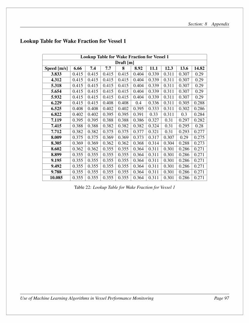
Section: 8 Appendix
Lookup Table for Wake Fraction for Vessel 1
Lookup Table for Wake Fraction for Vessel 1Draft [m]
Speed [m/s] 6.66 7.4 7.7 8 8.92 11.1 12.3 13.6 14.823.833 0.415 0.415 0.415 0.415 0.404 0.339 0.311 0.307 0.294.312 0.415 0.415 0.415 0.415 0.404 0.339 0.311 0.307 0.295.318 0.415 0.415 0.415 0.415 0.404 0.339 0.311 0.307 0.295.654 0.415 0.415 0.415 0.415 0.404 0.339 0.311 0.307 0.295.932 0.415 0.415 0.415 0.415 0.404 0.339 0.311 0.307 0.296.229 0.415 0.415 0.408 0.408 0.4 0.336 0.311 0.305 0.2886.525 0.408 0.408 0.402 0.402 0.395 0.333 0.311 0.302 0.2866.822 0.402 0.402 0.395 0.395 0.391 0.33 0.311 0.3 0.2847.119 0.395 0.395 0.388 0.388 0.386 0.327 0.31 0.297 0.2827.415 0.388 0.388 0.382 0.382 0.382 0.324 0.31 0.295 0.287.712 0.382 0.382 0.375 0.375 0.377 0.321 0.31 0.293 0.2778.009 0.375 0.375 0.369 0.369 0.373 0.317 0.307 0.29 0.2758.305 0.369 0.369 0.362 0.362 0.368 0.314 0.304 0.288 0.2738.602 0.362 0.362 0.355 0.355 0.364 0.311 0.301 0.286 0.2718.899 0.355 0.355 0.355 0.355 0.364 0.311 0.301 0.286 0.2719.195 0.355 0.355 0.355 0.355 0.364 0.311 0.301 0.286 0.2719.492 0.355 0.355 0.355 0.355 0.364 0.311 0.301 0.286 0.2719.788 0.355 0.355 0.355 0.355 0.364 0.311 0.301 0.286 0.271
10.085 0.355 0.355 0.355 0.355 0.364 0.311 0.301 0.286 0.271
Table 22: Lookup Table for Wake Fraction for Vessel 1
Use of Machine Learning Algorithms in Vessel Performance Monitoring Page 97

Section: 8 Appendix
Lookup Table for Thrust Deduction Factor for Vessel 1
Lookup Table for Thrust Deduction Factor for Vessel 1Draft [m]
Speed [m/s] 6.66 7.4 7.7 8 8.92 11.1 12.3 13.6 14.823.833 0.186 0.186 0.186 0.186 0.158 0.179 0.168 0.18 0.1994.312 0.186 0.186 0.186 0.186 0.158 0.179 0.168 0.18 0.1995.318 0.186 0.186 0.186 0.186 0.158 0.179 0.168 0.18 0.1995.654 0.186 0.186 0.186 0.186 0.158 0.179 0.168 0.18 0.1995.932 0.186 0.186 0.186 0.186 0.158 0.179 0.168 0.18 0.1996.229 0.186 0.186 0.184 0.184 0.158 0.178 0.168 0.182 0.1976.525 0.184 0.184 0.181 0.181 0.158 0.177 0.168 0.183 0.1956.822 0.181 0.181 0.178 0.178 0.158 0.175 0.168 0.185 0.1927.119 0.178 0.178 0.175 0.175 0.158 0.174 0.168 0.187 0.197.415 0.175 0.175 0.172 0.172 0.158 0.173 0.168 0.189 0.1887.712 0.172 0.172 0.17 0.17 0.158 0.172 0.172 0.19 0.1868.009 0.17 0.17 0.167 0.167 0.158 0.171 0.173 0.192 0.1848.305 0.167 0.167 0.164 0.164 0.158 0.169 0.174 0.194 0.1828.602 0.164 0.164 0.161 0.161 0.158 0.168 0.175 0.196 0.1798.899 0.161 0.161 0.161 0.161 0.158 0.168 0.175 0.196 0.1799.195 0.161 0.161 0.161 0.161 0.158 0.168 0.175 0.196 0.1799.492 0.161 0.161 0.161 0.161 0.158 0.168 0.175 0.196 0.1799.788 0.161 0.161 0.161 0.161 0.158 0.168 0.175 0.196 0.179
10.085 0.161 0.161 0.161 0.161 0.158 0.168 0.175 0.196 0.179
Table 23: Lookup Table for Thrust Deduction Factor for Vessel 1
Use of Machine Learning Algorithms in Vessel Performance Monitoring Page 98

Section: 8 Appendix
Open Water Efficiency Propeller Curve for Vessel 1
Figure 53: ηO Propeller Open Water Efficiency curve for Propeller of Vessel 1, Generated as StandardWageningen B -Series Propeller
Inputs to generate RAO to calculate the Added Resistance in Waves15
Inputs to generate RAO15
Data Used UnitLength [m]Breadth [m]Draft [deg]Block CoefficientWave Direction [deg]Ship Speed [m/s]
Table 24: Inputs to generate RAO to calculate the Added Resistance in Waves15
Use of Machine Learning Algorithms in Vessel Performance Monitoring Page 99

Section: 8 Appendix
Tabulated Values of MAE and R2 for Vessel 1 - Linear Regression
1st Model 2nd Model 3rd ModelUniversal Model MAE R2 MAE R2 MAE R2
Surface Roughness [µm] 571.64 0.58 629 0.64 628.15 0.64Fouling Resistance [kN] 49.89 0.73 43.71 0.77 44.16 0.77
Separated ModelsSurface Roughness [µm] 397.41 0.74 429.17 0.75 428.63 0.75Fouling Resistance [kN] 37.93 0.82 35.23 0.83 35.13 0.84
Chosen Data Range(From Period 1 to 2 mid)Surface Roughness [µm] 496.43 0.67 640.89 0.70 605.14 0.71Fouling Resistance [kN] 44.52 0.74 41.52 0.76 39.87 0.78
Table 25: Tabulated Values of MAE and R2 for Vessel 1 - Linear Regression
Use of Machine Learning Algorithms in Vessel Performance Monitoring Page 100

Section: 8 Appendix
Tabulated Values of MAE and R2 for Vessel 1 - LSTM
LSTM - Fit and Error - For Vessel 1 MAE R2
1st ModelUniversal Model
Surface Roughness [µm] 480.95 0.50Fouling Resistance [kN] 43.98 0.81
2nd ModelUniversal Model
Surface Roughness [µm] 421.74 0.64Fouling Resistance [kN] 39.26 0.85
From Period 2-4Surface Roughness [µm] 478.66 0.60Fouling Resistance [kN] 43.52 0.74
From Period 3-4Surface Roughness [µm] 587.15 0.32Fouling Resistance [kN] 64.31 0.47
3rd ModelUniversal Model
Surface Roughness [µm] 374.95 0.70Fouling Resistance [kN] 35.01 0.87
From Period 2-4Surface Roughness [µm] 409.53 0.65Fouling Resistance [kN] 36.34 0.82
From Period 3-4Surface Roughness [µm] 445.66 0.54Fouling Resistance [kN] 38.59 0.81
Table 26: Tabulated Values of MAE and R2 for Vessel 1 - LSTM
Use of Machine Learning Algorithms in Vessel Performance Monitoring Page 101

DTU Mechanical EngineeringSection of Fluid Mechanics, Coastal and Maritime EngineeringTechnical University of Denmark
Nils Koppels Allé, Bld. 403DK-2800 Kgs. Lyngby Denmark
Tlf.: +45 4525 1360Fax: +45 4525 1961
www.mek.dtu.dk
July 2020