us in g ord e red weight av e raging (owa) for … · 1 us in g ord e red weight av e raging (owa)...

1

USING ORDERED WEIGHT AVERAGING (OWA) FOR MULTICRITERIA SOIL

FERTILITY EVALUATION BY GIS (CASE STUDY: SOUTHEAST IRAN)

Marzieh Mokarram1*, Majid Hojati2

5 1*Department of Range and Watershed Management, College of Agriculture and Natural Resources of Darab, Shiraz

University, Iran, Email: [email protected]

2Department of GIS and RS, University of Tehran, Faculty of Geography, Dep. of RS & GIS,

Email:[email protected]

Corresponding author: Marzieh Mokarram, Tel.: +98-917-8020115; Fax: +987153546476 , Address: Darab, 10

Shiraz university, Iran, Postal Code: 71946-84471, Email: [email protected]

Abstract

The Multicriteria Decision Analysis (MCDA) and Geographical Information Systems (GIS) are used to

provide accurate information on Pedogenic processes and facilitate the work of decision makers. So,

MCDA and GIS, can provide a wide range of decision strategies or scenarios in some procedures. One 15

of the popular algorithm of multicriteria analysis is Ordered Weighted Averaging (OWA). The OWA

procedure depends on some parameters, which can be specified by means of fuzzy. The aim of this

study is to take the advantage of the incorporation of fuzzy into GIS-based soil fertility analysis by

OWA in west Shiraz, Fars province, Iran. For the determination of soil fertility maps, OWA

parameters such as potassium (K), phosphor (P), copper (Cu), iron (Fe), manganese (Mn), organic 20

carbon (OC) and zinc (Zn) were used. After generated interpolation maps with Inverse Distance

Weighted (IDW), fuzzy maps for each parameter were generated by the membership functions. Finally,

with OWA six maps for fertility with different risk level were made. The results show that with

decreasing risk (no trade-off), almost all of the parts of the study area were not suitable for soil fertility.

While increasing risk, more area was suitable in terms of soil fertility in the study area. So using OWA 25

can generate many maps with different risk levels that lead to different management due to the different

financial conditions of farmers.

Keywords: Multicriteria Decision Analysis (MCDA); Ordered weighted averaging (OWA); fuzzy; Soil fertility.

Solid Earth Discuss., doi:10.5194/se-2016-17, 2016Manuscript under review for journal Solid EarthPublished: 2 March 2016c© Author(s) 2016. CC-BY 3.0 License.

2

1. Introduction

Spatial planning involves decision-making techniques that are associated with techniques such as Multi 30

Criteria Decision Analysis (MCDA) and multicriteria Evaluation (MCE). Combining GIS with MCDA

methods creates a powerful tool for spatial planning (Malczewski, 1999; Shumilov et al., 2011; Kanokporn

& Iamaram, 2011; Belkhiri et al., 2011; Salehi et al., 2012; Feng et al., 2012; Ashrafi et al., 2012).

Multicriteria evaluation may be used to develop and evaluate alternative plans that may facilitate

compromise among interested parties (Malczewski, 1996). In general, the GIS-based soil fertility 35

analysis assumes that a given study area is subdivided into a set of basic units of observation such as

polygons or rasters. Then, the soil fertility problem involves evaluation and classification of the areal

units according to their fertility for a particular activity. There are two fundamental classes of

multicriteria evaluation methods in GIS: The Boolean overlay operations (none compensatory

combination rules) and the weighted linear combination (WLC) methods (compensatory combination 40

rules). These approaches can be generalized within the framework of the ordered weighted averaging

(OWA) (Asproth et al., 1999; Jiang and Eastman, 2000; Makropoulos et al., 2003; Malczewski et al.,

2003; Malczewski & Rinner, 2005; Malczewski .,2006). OWA is a family of multicriteria combination

procedures (Yager, 1988). Conventional OWA can utilizes the qualitative statements in the form of

fuzzy quantifiers (Yager, 1988, 1996). The main goal of this paper is to produce the land suitability 45

maps according to OWA operators for GIS-based multicriteria evaluation procedures.

OWA has been developed as a popularization of multicriteria combination by Yager (1988). The OWA

concept has been extended to the GIS applications by Eastman (1997) as a part of decision support

module in GIS-IDRISI. Subsequently, Jiang and Eastman (2000) demonstrate the utility of the GIS-

OWA for land use/suitability problems. The implementation of the OWA concept in IDRISI15.01 50

resulted in several applications of OWA to environmental a n d urban planning problems (Asprothet

al., 1999; Mendes & Motizuki, 2001).


3

Mokarram and Aminzadeh (2010) used OWA for land suitability in Shavur plain, Iran. The results

showed that OWA is a multicriteria evaluation procedure (or combination operator). The quantifier-

guided OWA procedure is illustrated using land-use suitability analysis in Shavur plain, Iran. 55

Liu and Malczewski (2013) used GIS-Based Local Ordered Weighted Averaging in London, Ontario. In

the study area, the aim was to implement local form of OWA. The local model was based on the range

sensitivity principle. The results showed that there were substantial differences between the spatial

patterns generated by the global and local OWA methods.

Accordingly, the study area is one of the most important centers of agriculture in Iran, and the aim of 60

the study is the determination of produce the soil fertility maps according to OWA operators for GIS-

based multicriteria evaluation procedures in southeast Iran using OWA. In the study, we expected

that the selected OWA method is the best method for the determination of multicriteria soil

fertility. According to OWA method the amount of soil fertility with different risk levels was

determined that is useful for farmers with different financial conditions. 65

2. Methods

In order to prepare soil fertility maps using OWA method, 45 sample soils were used that after the

creation of the interpolation maps for each parameters using Inverse Distance Weighted (IDW) and the

creation of a fuzzy parameter map for each parameter, in order to make different risk levels OWA was 70

used. The description of each method is in the following:

2.1. Inverse Distance Weighted (IDW)

IDW model was used for interpolating Effective data in determining of soil fertility such as potassium

(K), phosphor (P), copper (Cu), iron (Fe), manganese (Mn), organic carbon (OC) and zinc (Zn). IDW

interpolation explicitly implements the assumption that things that are close to one another are more 75

alike than those that are farther apart. To predict a value for any unmeasured location, IDW will use the


4

measured values surrounding the prediction location. Assumes value of an attribute z at any unsampled

point is a distance-weighted average of sampled points lying within a defined neighborhood around

that unsampled point. Essentially it is a weighted moving average (Burrough, et al., 1998):

80

10

1

( )d

ˆ( )

d

nr

i ij

i

nr

ij

i

z x

z x

(1)

Where x0 is the estimation point and xi are the data points within a chosen neighborhood. The weights

(r) are related to distance by dij.

85

2.2. Ordered Weight Average (OWA)

OWA is a multicriteria evaluation procedure. The nature of the OWA procedure depends on some

parameters, which can be specified by fuzzy quantifiers. The GIS-based multicriteria evaluation

procedures involve a set of spatially defined alternatives and a set of evaluation criteria represented as

map layers. According to the input data (criterion weights and criterion map layers), the OWA 90

combination operator associates with the i- th location (e.g., raster or point) a set of order weights v =

v1, v2, . . ., vn such that vj [0, 1], j=1, 2..., n, 1

1N

j

j

v

, and is defined as follows (see Yager, 1988;

Malczewski et al., 2003):

1

1

u v( )

u v

Nj j

t tfnj

j j

j

OWA z

(2)

where zi1 ≥ zi2 ≥ . . . ≥ zin is the sequence obtained by reordering the attribute values ai1, ai2, . . ., ain, and 95

uj is the criterion weight reordered according to the attribute value, zij. It is important to point to the

difference between the two types of weights (the criterion weights and the order weights). The criterion


5

weights are assigned to evaluation criteria to indicate their relative importance. All locations on the j-th

criterion map are assigned the same weight of wj. The order weights are associated with the criterion

values on the location-by-location basis. They are assigned to the i-th location’s attribute value in 100

decreasing order without considering from which criterion map the value comes. With different sets of

order weights, one can generate a wide range of OWA operators including the most often used GIS-

base map combination procedures: the weighted linear combination (WLC) and Boolean overlay

operations, such as intersection (AND) and union (OR) (Yager, 1988; Malczewski et al., 2003). The

AND and OR operators represent the extreme cases of OWA and they correspond to the MIN and MAX 105

operators, respectively. The order weights associated with the MIN operator are: vn = 1, and vj = 0 for

all other weights. Given the order weights, OWAi (MIN) = MINj (ai1, ai2, . . ., ain). The following

weights are associated with the MAX operator: v1 = 1, and vj = 0 for all other weights, and consequently

OWAi (MAX) = MAXj (ai1, ai2, . . ., ain). Assigning equal order weights (that is, vj = 1/n for j = 1, 2, . . .

, n) results in the conventional WLC, which is situated at the mid-point on the continuum ranging from 110

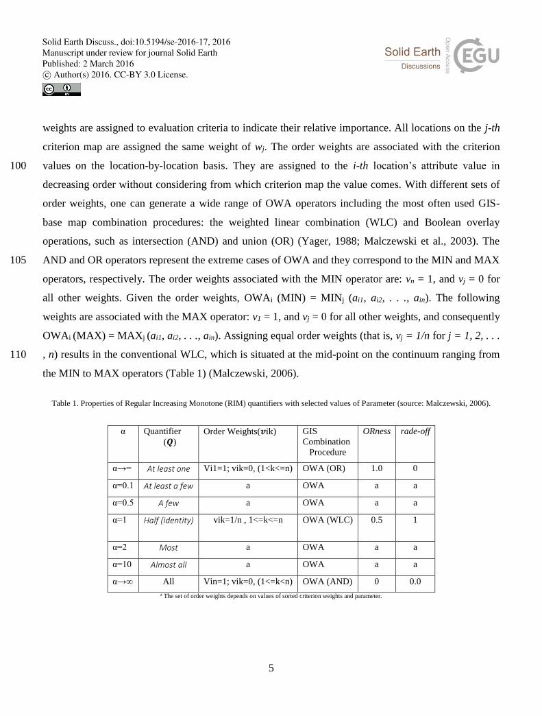
the MIN to MAX operators (Table 1) (Malczewski, 2006).

Table 1. Properties of Regular Increasing Monotone (RIM) quantifiers with selected values of Parameter (source: Malczewski, 2006).

α Quantifier

(𝑸)

Order Weights(𝒗ik) GIS

Combination

Procedure

ORness

rade-off

α→= At least one Vi1=1; vik=0, (1<k<=n) OWA (OR) 1.0 0

α=0.1 At least a few a OWA a a

α=0.5 A few a OWA a a

α=1 Half (identity)

vik=1/n , 1<=k<=n OWA (WLC) 0.5 1

α=2 Most a OWA a a

α=10 Almost all a OWA a a

α→∞ All Vin=1; vik=0, (1<=k<n) OWA (AND) 0 0.0

a The set of order weights depends on values of sorted criterion weights and parameter.


6

3. Case study 115

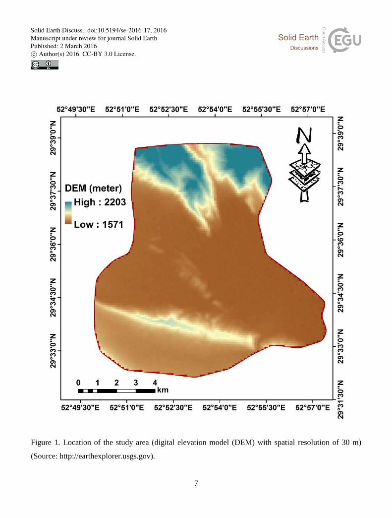
This study was carried out in west Shiraz, Fars province, Iran. It is an area of about 100.02 km2, and is

located at longitude of N 29° 31΄- 29° 38΄and latitude of E 52° 49΄ to 52° 57΄ (Figure 1). The altitude of

the study area ranges from the lowest of 1,571 m to the highest of 2,203 m. The main agricultural

produce consists of grain, fruit, and vegetables, while the partly wooded mountains are used for

pasture. 120


7

Figure 1. Location of the study area (digital elevation model (DEM) with spatial resolution of 30 m)

(Source: http://earthexplorer.usgs.gov).


8

The assessment of soil fertility for agricultural production in the region is vital, which should consider 125

environmental factors and human conditions (Soufi, 2004). In order to predict the variability of soil

fertility, P, K, Cu, Fe, Mn, OC and Zn maps were prepared (Table 2) (Organization of Agriculture

Jahad Fars province).

Table 2. Descriptive statistics of the data for soil fertility (Organization of Agriculture Jahad Fars

province) 130

Statistic

parameters

OC

(mg/kg)

P

(mg/kg)

K

(mg/kg)

Fe

(mg/kg)

Zn

(mg/kg)

Mn

(mg/kg)

Cu

(mg/kg)

maximum 1.65 30.00 666.00 15.00 3.00 52.50 2.00

minimum 0.18 2.00 137.00 1.00 0.10 2.80 0.20

average 1.01 13.94 313.73 4.54 0.65 14.77 0.97

STDEV 0.35 6.49 104.28 2.84 0.50 10.71 0.36

4. Results and Discussion

4.1. Inverse Distance Weighted (IDW)

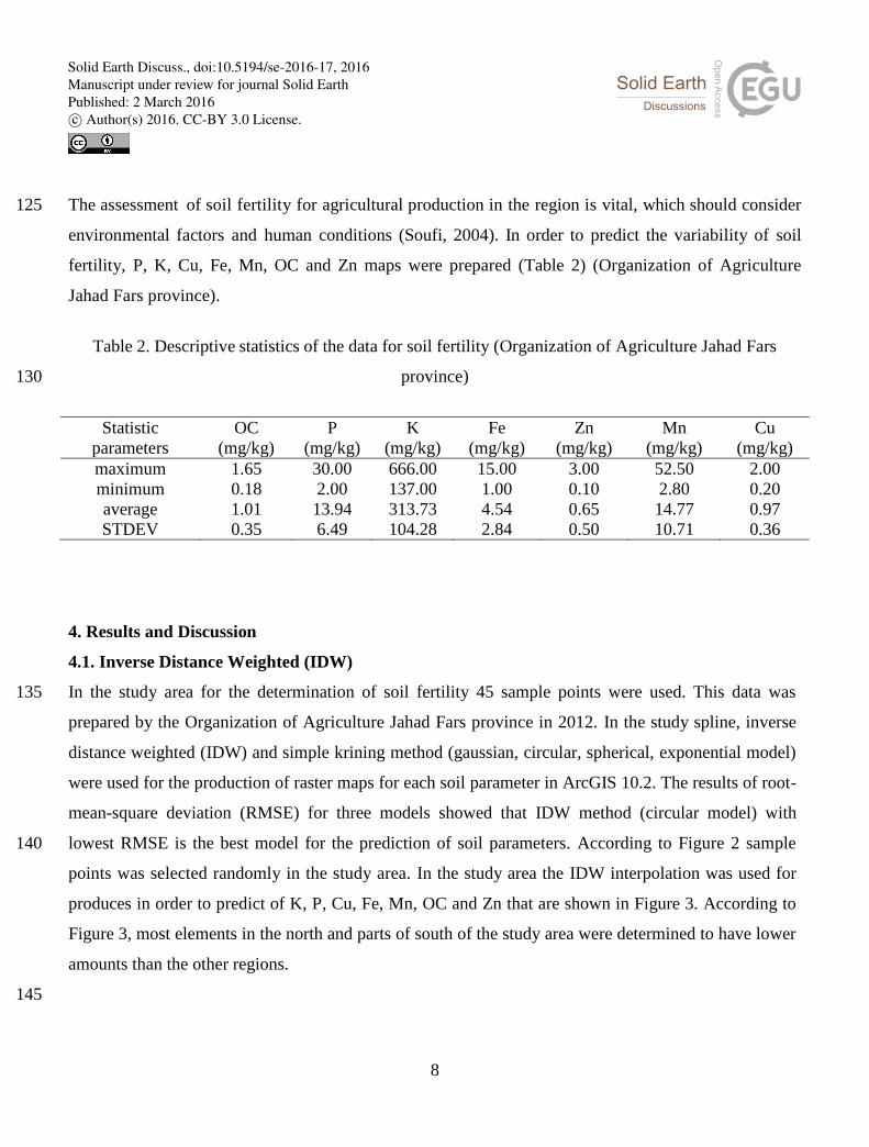
In the study area for the determination of soil fertility 45 sample points were used. This data was 135

prepared by the Organization of Agriculture Jahad Fars province in 2012. In the study spline, inverse

distance weighted (IDW) and simple krining method (gaussian, circular, spherical, exponential model)

were used for the production of raster maps for each soil parameter in ArcGIS 10.2. The results of root-

mean-square deviation (RMSE) for three models showed that IDW method (circular model) with

lowest RMSE is the best model for the prediction of soil parameters. According to Figure 2 sample 140

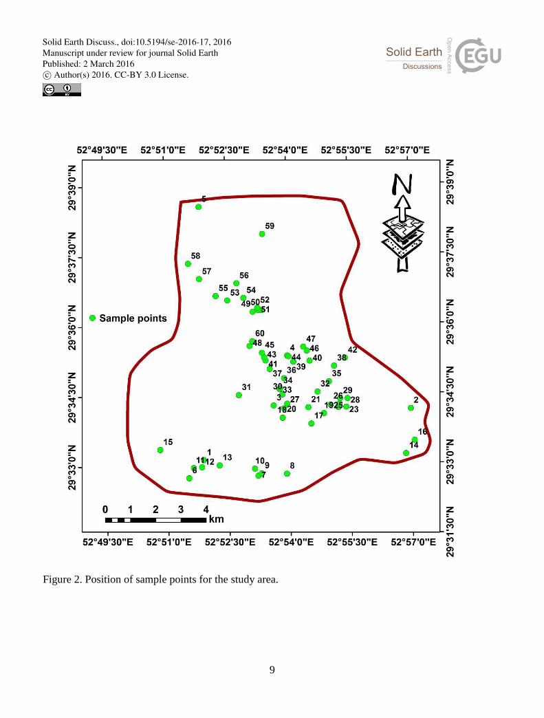
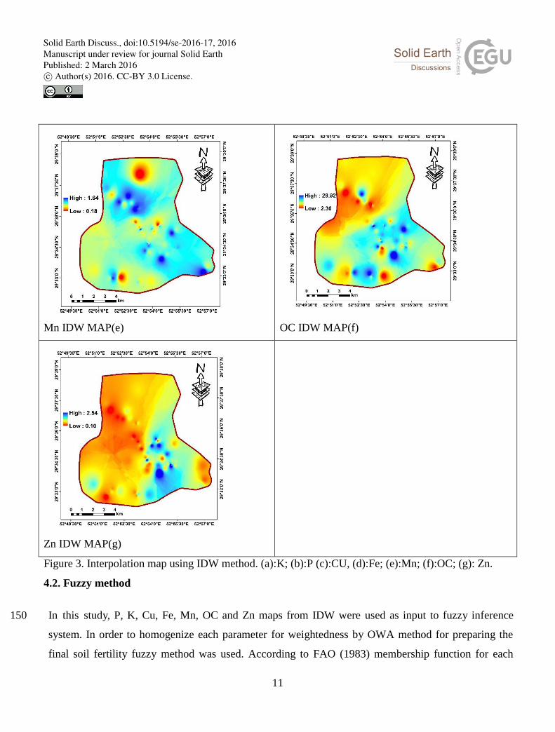
points was selected randomly in the study area. In the study area the IDW interpolation was used for

produces in order to predict of K, P, Cu, Fe, Mn, OC and Zn that are shown in Figure 3. According to

Figure 3, most elements in the north and parts of south of the study area were determined to have lower

amounts than the other regions.

145


9

Figure 2. Position of sample points for the study area.


10

Potassium (K) IDW Map(a)

Phosphor (P) IDW Map(b)

Cu IDW Map (c)

Fe IDW Map(d)


11

Mn IDW MAP(e)

OC IDW MAP(f)

Zn IDW MAP(g)

Figure 3. Interpolation map using IDW method. (a):K; (b):P (c):CU, (d):Fe; (e):Mn; (f):OC; (g): Zn.

4.2. Fuzzy method

In this study, P, K, Cu, Fe, Mn, OC and Zn maps from IDW were used as input to fuzzy inference 150

system. In order to homogenize each parameter for weightedness by OWA method for preparing the

final soil fertility fuzzy method was used. According to FAO (1983) membership function for each


12

parameter was defined (K, P, Cu, Fe, Mn, OC and Zn) and each of fuzzy map was created for each

elements between 0 to 1. The prepared fuzzy maps for the soil fertility parameters are shown in Figure

4, where MF is closer to 0 with decreasing soil fertility, while MF is closer to 1 with increasing soil 155

fertility (Soroush et al., 2011).

Potassium (K) Fuzzy Map(a)

Phosphor (P) Fuzzy Map(b)

Cu Fuzzy Map (c)

Fe Fuzzy Map(d)


13

Mn Fuzzy MAP (e)

OC Fuzzy MAP (f)

Zn Fuzzy MAP (g)

Figure 4. Fuzzy map of studied area for each soil fertility parameter. (a):K; (b):P (c):CU, (d):Fe;

(e):Mn; (f):OC; (g): Zn.

160

According to Figure 4 most of the study area did not have a suitable value for Mn parameter that in the

fuzzy map had the value close to zero (critical limit =10 (mg/kg)). While the results of fuzzy method

showed that most of the study area (the parts of east, southeast and the small parts of south west of the

study area) had suitable values for P and Zn parameters that had the value close to 1 in fuzzy map

(critical limit= and for P and Zn respectively). Parts of north, south west and south of the study area 165


14

were not suitable for fertility (critical limit=). According to the fuzzy map of K parts of north, southeast

and west were not suitable (critical limit=). Also parts of north, northwest and south of the study area

were not suitable for Cu. Finally it was determined that only parts of northeast, southeast and the small

parts of west and east were suitable for soil fertility.

170

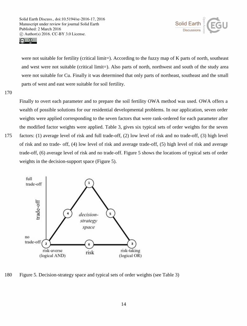
Finally to overt each parameter and to prepare the soil fertility OWA method was used. OWA offers a

wealth of possible solutions for our residential developmental problems. In our application, seven order

weights were applied corresponding to the seven factors that were rank-ordered for each parameter after

the modified factor weights were applied. Table 3, gives six typical sets of order weights for the seven

factors: (1) average level of risk and full trade-off, (2) low level of risk and no trade-off, (3) high level 175

of risk and no trade- off, (4) low level of risk and average trade-off, (5) high level of risk and average

trade-off, (6) average level of risk and no trade-off. Figure 5 shows the locations of typical sets of order

weights in the decision-support space (Figure 5).

Figure 5. Decision-strategy space and typical sets of order weights (see Table 3) 180


15

Table 3: Typical sets of order weights for seven factors.

(1) Average level of risk and full trade-off

order weight 0.1428 0.1428 0.1428 0.1428 0.1428 0.1428 0.1428

rank 1st 2nd 3rd 4th 5th 6th 7th

(2) Low level of risk and no trade-off

order weight 1 0 0 0 0 0 0


(3) High level of risk and no trade-off



(4) Low level of risk and average trade-off

order weight 0.4455 0.2772 0.1579 0.0789 0.0320 0.0085 0


(5) High level of risk and average trade-off

order weight 0 0.0085 0.032 0.0789 0.1579 0.2772 0.4455


(6) Average level of risk and no trade-off



Given the standardized criterion maps and corresponding criterion weights, we apply the OWA 185

operator using Eq. (2) for selected values of fuzzy quantifiers: at least one, at least a few, a few,

identity, most, almost all, and all are used. Each quantifier is associated with a set of order weights that

are calculated according to Eq. (2). Figure 6 shows the six alternative soil fertility patterns.


16


17

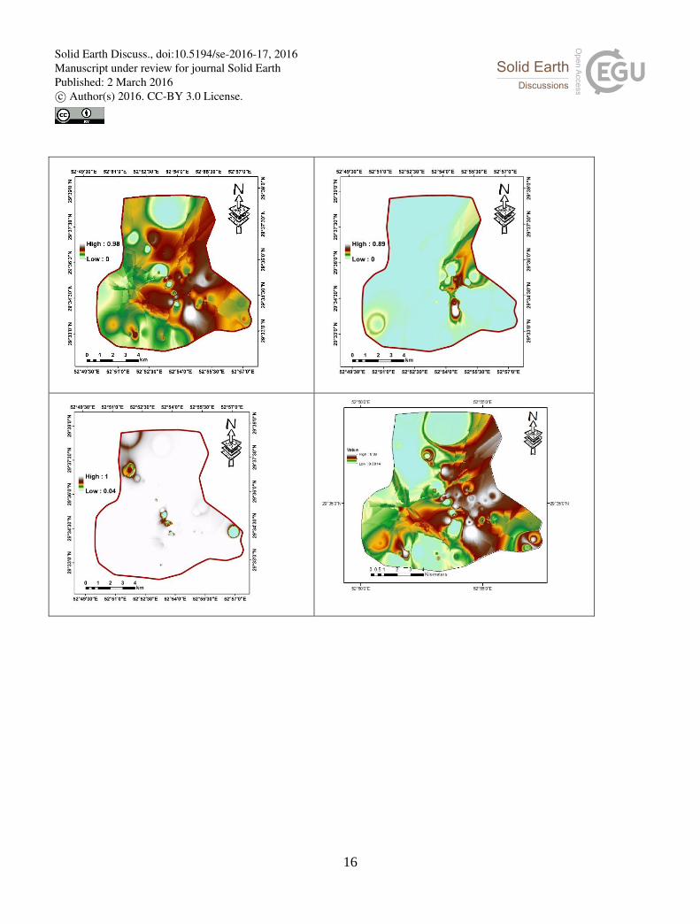
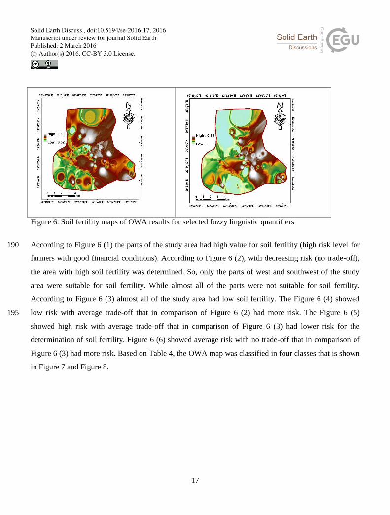
Figure 6. Soil fertility maps of OWA results for selected fuzzy linguistic quantifiers

According to Figure 6 (1) the parts of the study area had high value for soil fertility (high risk level for 190

farmers with good financial conditions). According to Figure 6 (2), with decreasing risk (no trade-off),

the area with high soil fertility was determined. So, only the parts of west and southwest of the study

area were suitable for soil fertility. While almost all of the parts were not suitable for soil fertility.

According to Figure 6 (3) almost all of the study area had low soil fertility. The Figure 6 (4) showed

low risk with average trade-off that in comparison of Figure 6 (2) had more risk. The Figure 6 (5) 195

showed high risk with average trade-off that in comparison of Figure 6 (3) had lower risk for the

determination of soil fertility. Figure 6 (6) showed average risk with no trade-off that in comparison of

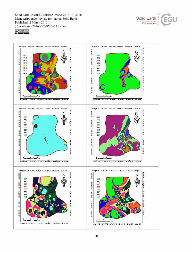
Figure 6 (3) had more risk. Based on Table 4, the OWA map was classified in four classes that is shown

in Figure 7 and Figure 8.


18


19

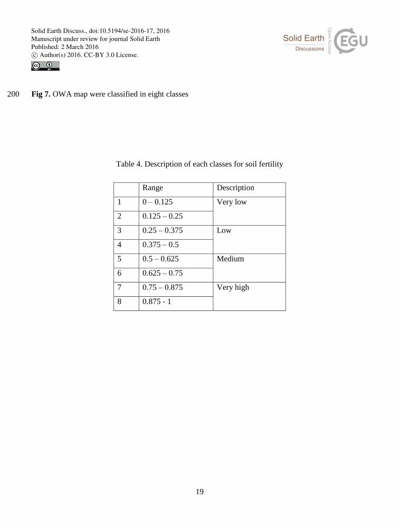
Fig 7. OWA map were classified in eight classes 200

Table 4. Description of each classes for soil fertility

Range Description

1 0 – 0.125 Very low

2 0.125 – 0.25

3 0.25 – 0.375 Low

4 0.375 – 0.5

5 0.5 – 0.625 Medium

6 0.625 – 0.75

7 0.75 – 0.875 Very high

8 0.875 - 1


20

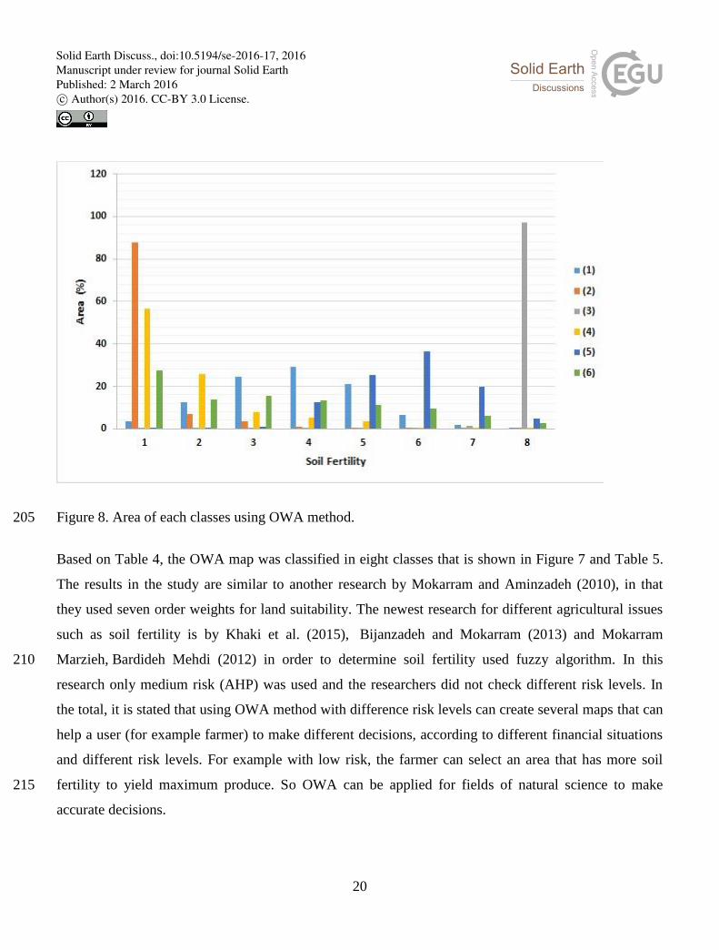
Figure 8. Area of each classes using OWA method. 205

Based on Table 4, the OWA map was classified in eight classes that is shown in Figure 7 and Table 5.

The results in the study are similar to another research by Mokarram and Aminzadeh (2010), in that

they used seven order weights for land suitability. The newest research for different agricultural issues

such as soil fertility is by Khaki et al. (2015), Bijanzadeh and Mokarram (2013) and Mokarram

Marzieh, Bardideh Mehdi (2012) in order to determine soil fertility used fuzzy algorithm. In this 210

research only medium risk (AHP) was used and the researchers did not check different risk levels. In

the total, it is stated that using OWA method with difference risk levels can create several maps that can

help a user (for example farmer) to make different decisions, according to different financial situations

and different risk levels. For example with low risk, the farmer can select an area that has more soil

fertility to yield maximum produce. So OWA can be applied for fields of natural science to make 215

accurate decisions.


21

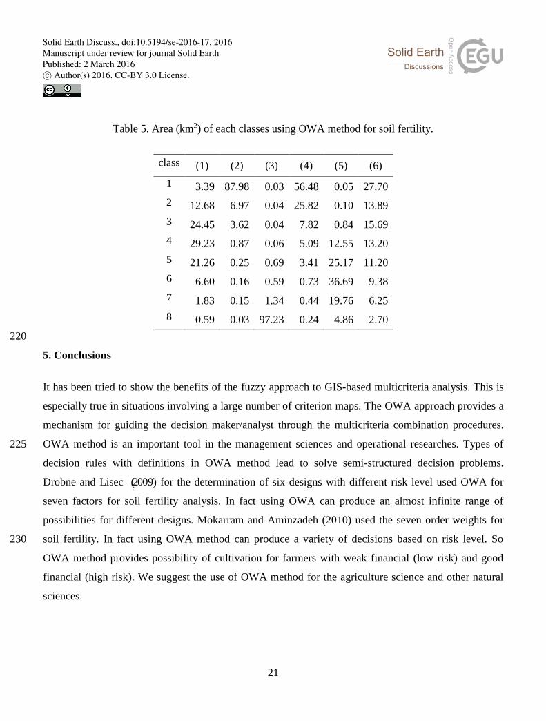
Table 5. Area (km2) of each classes using OWA method for soil fertility.

class (1) (2) (3) (4) (5) (6)

1 3.39 87.98 0.03 56.48 0.05 27.70

2 12.68 6.97 0.04 25.82 0.10 13.89

3 24.45 3.62 0.04 7.82 0.84 15.69

4 29.23 0.87 0.06 5.09 12.55 13.20

5 21.26 0.25 0.69 3.41 25.17 11.20

6 6.60 0.16 0.59 0.73 36.69 9.38

7 1.83 0.15 1.34 0.44 19.76 6.25

8 0.59 0.03 97.23 0.24 4.86 2.70

220

5. Conclusions

It has been tried to show the benefits of the fuzzy approach to GIS-based multicriteria analysis. This is

especially true in situations involving a large number of criterion maps. The OWA approach provides a

mechanism for guiding the decision maker/analyst through the multicriteria combination procedures.

OWA method is an important tool in the management sciences and operational researches. Types of 225

decision rules with definitions in OWA method lead to solve semi-structured decision problems.

Drobne and Lisec (2009) for the determination of six designs with different risk level used OWA for

seven factors for soil fertility analysis. In fact using OWA can produce an almost infinite range of

possibilities for different designs. Mokarram and Aminzadeh (2010) used the seven order weights for

soil fertility. In fact using OWA method can produce a variety of decisions based on risk level. So 230

OWA method provides possibility of cultivation for farmers with weak financial (low risk) and good

financial (high risk). We suggest the use of OWA method for the agriculture science and other natural

sciences.


22

References 235

1. Ashrafi, Kh., Shafiepour, M. Ghasemi, L. and B. NajarAraabi. 2012. Prediction of Climate

Change Induced Temperature Rise in Regional Scale Using Neural Network, International

Journal of Environmental Research 6 (3), 677-688.

2. Asproth , V. , Holm berg, S. C. a n d A. Håka nsson. 1 99 9. D e c is io n sup po rt f or s p at ia l

pla n ning and management of human settlements’, in Lasker, G.E. (Ed.): Advances in Support 240

Systems Research, Vol. 5, International Institute for Advanced Studies in Systems Research

and Cybernetics, Windsor, Ontario, Canada, pp.30–39.

3. Basso, B., De Simone, L.,Cammarano, D., Martin, E.C., Margiotta, S., Grace, P.R.,Yeh, M.L.

and T.Y. Chou. 2012. E valu ating Responses to Land D egradation Mitigation Measures in

Southern Italy, International Journal of Environmental Research 6 (2), 367-380. 245

4. Beedasy, J., and D. Whyatt. 1999. Diverting the tourists: aspatial decisionsupport system for

tourism planning on a developing island. Journal of Apply Earth Observ. Geoinformation. 3/4,

163–174.

5. Belkhiri, L., Boudoukha, A., an d L. Mouni. 2011. A multivariate Statistical Analysis of

Groundwater Chemistry Data, International Journal of Environmental Research 5 (2), 537-250

544.

6. Burrough, P.A., and R.A. McDonnell. 1998. Principles of geographical information systems.

Spatial Information System and Geostatistics. Oxford University Press, New York.

7. Eastman, J. R. 1997. IDRISI for Windows, Version 2.0: Tutorial Exercises, Graduate School

of Geography, Clark University, Worcester. 255

8. Feng, X.Y., and Luo, G.P., Li, C.F., Dai, L. and L. Lu. 2012.Dynamics of Ecosystem Service

Value Caused by Land use Changes in ManasRiver of Xinjiang, China, International Journal

of Environmental Research 6 (2), 499-508.

9. Fumagalli, N. and A. Toccolini. 2012. Relationship Between Greenways and Ecological

Network: A Case Study in Italy, International Journal of Environmental Research 6 (4), 903-260

916.


23

10. Organization of Agriculture Jahad Fars province (http://www.fajo.ir).

11. Jiang, H., and J.R. Eastman. 2000. Application of fuzzy measures in multi-criteria evaluation in

GIS. International Journal of Geography Information System 14, 173–184.

12. Kanokporn, K. and V. Iamaram. 2011. Ecological Impact Assessment; Conceptual Approach 265

for Better Outcomes, Int. J. Environ. Res., 5 (2), 435-446.

13. Kim, D.K., Jeong, K.S., McKay, R.I.B., Chon, T. S. and G. J. Joo . 2 01 2. M a chine Learning

for Predict iv e Management: Short and L on g term Prediction of Phytoplankton Biom ass u

sing Genetic Algorithm Based Recurrent Neural Networks, International Journal of

Environmental Research 6 (1), 95-108. 270

14. Liu, X., J. Malczewski. 2013. GIS-Based Local Ordered Weighted Averaging: A Case Study in

London, Ontario. Electronic Thesis and Dissertation Repository. Paper 1227.

15. Makropoulos, C., Butler, D., and C. Maksimovic. 2003. A fuzzy logic spatial decision support

system for urban water management. J. Water Resour. Plann. Manage. 129 (1),69–77.

16. Malczewski, J. 2006. Ordered weighted averaging with fuzzy quantifiers: GIS-based 275

multicriteria evaluation for land-use suitability analysis. International Journal of Applied Earth

Observation and Geoinformation. 8: 270–277.

17. Malczewski, J. 1996. A GIS-based approach to multiplecriteria group decision making.

International Journal of Geographical Information Systems 10(8), 955-971.

18. Malczewski, J. 1999. GIS and Multicriteria Decision Analysis. John Wiley & Sons Inc., New 280

York.

19. Malczewski, J. 2004. GIS-based land-use suitability analysis: a critical overview. Progr. Plann.

62 (1), 3–65.

20. Malczewski, J., Chapman, T., Flegel, C., Walters, D., Shrubsole, D., and M.A. Healy. 2003.

GIS-multicriteria evaluation with ordered weighted averaging (OWA): case study of developing 285

watershed management strategies. Environ. Plann. A 35 (10), 1769–1784.

21. Malczewski, J., and C. Rinner. 2005. Exploring multicriteria decision strategies in GIS with

linguistic quantifiers: a case study of residential quality evaluation. Journal of Geography

System 7 (2), 249–268.


24

22. Mendes, J.F.G. and W.S. Motizuki. 2001.Urban quality of life evaluation scenarios: the case 290

of sãocarlos in Brazil. CTBUH Review, 1 (2), 1–10.

23. Mokarram M., and F. Aminzadeh. 2010. GIS-based multicriteria land suitability evaluation

using ordered weight averaging with fuzzy quantifier: a case study in Shavur plain, Iran. The

International Archives of the Photogrammetry, Remote Sensing and Spatial Information

Sciences, Vol. 38, Part II. 295

24. Nejadi, A., Jafari, H.R., Makhdoum, M. F. and M. Mahmoudi. 2012.Modeling Plausible

Impacts of land use change on w ildlife h abitats, Application an d validation : Lisar

protected area, Iran, International Journal of Environmental Research 6 (4), 883-892.

25. Rasouli, S., MakhdoumFarkhondeh, M., Jafari, H .R., Suffling,R., Kiabi, B. and A. R.

Yavari. 2012. Assessment of Ecological integrity in a landscape con text using the 300

Miankalepeninsula of Northern Iran, Int. J. Environ. Res., 6 (2), 443-450.

26. Salehi, E., Zebardast, L. and A. R. Yavri. 2012. Detecting Forest Fragmentation with

Morphological Image Processing in Golestan National Park in northeast of Iran, International

Journal of Environmental Research 6 (2), 531-536.

27. Sanaee., M. FallahShamsi, S. R. and H. FerdowsiAsemanjerdi. 2010. Multi-criteria land 305

evaluation, using WLC and OWA strategies to select suitable site of forage plantation (Case

study; Zakherd, Fars). Rangeland, 4 (2), 216-227.

28. Shumilov, O.I., Kasatkina, E.A., Mielikainen, K., Timonen, M. and A.G. Kanatjev. 2011.

Palaeovolcanos, Solar activity and pine tree-rings from the Kola Peninsula (northwestern

Russia) over the last 560 years, International Journal of Environmental Research 5 (4),855-310

864.

29. Soufi M. 2004. Morpho-climatic classification of gullies in fars province, southwest of i.r. iran .

International Soil Conservation Organisation Conference – Brisbane.

30. Yager, R.R. 1988. On ordered weighted averaging aggregation operators in multi-criteria

decision making. IEEE Trans. Syst. Man Cybernet. 18 (1), 183–190. 315

31. Yager, R.R. 1996. Quantifier guided aggregation using OWA operators. Int. J. Intell. Syst. 11,

49–73.


25

32. Drobne, S., Lisec A. 2009. Multi-attribute Decision Analysis in GIS: Weighted Linear

Combination and Ordered Weighted Averaging. Informatica 33 (2009) 459–474.

33. B. Delsouz Khaki, N. Honarjoo, N. Davatgar, A.Jalalian, H. Torab. 2015. Soil Fertility Evaluation 320

Using Fuzzy Membership Function (Case Study: Southern Half of Foumanat Plain in North of

Iran). Allgemeine forst undjagdzeitung. 53-64P.

34. Mokarram M, Bardideh M. 2012. Soil fertility evaluation for wheat cultivation by fuzzy theory

approache and compared with boolean method and soil test method in gis area. Agronomy

journal (pajouhesh & sazandegi). Volume 25 , number 3 (96); page(s) 111 -123. 325

35. Bijanzadeh E, Mokarram, M. 2013. The use of fuzzy- AHP methods to assess fertility classes for

wheat and its relationship with soil salinity: east of Shiraz, Iran : A case study. AUSTORALIUN

journal of crop science. 7(11):1699-1706

330


26

Figure captions

Figure 1. Location of the study area (digital elevation model (DEM) with spatial resolution of 30 m)

(Source: http://earthexplorer.usgs.gov). 335

Figure 2. Position of sample points for the study area.

Figure 3. Interpolation map using IDW method. (a):Cu; (b):Fe; (c):K; (d):Mn; (e):OC; (f):P; (g): Zn.

Figure 4. Fuzzy map of studied area for each soil fertility parameter. (a):Cu; (b):Fe; (c):K; (d):Mn;

(e):OC; (f):P; (g): Zn.

Figure 5. Decision-strategy space and typical sets of order weights (see Table 3) 340

Figure 6. Soil fertility maps of OWA results for selected fuzzy linguistic quantifiers

Figure 7. Classification of OWA map for soil fertility.

Figure 8. Area of each classes using OWA method.

345


us in g ord e red weight av e raging (owa) for … · 1 us in g ord e red weight av e raging (owa)...

Documents