u.s. drive fuels working group engine and vehicle modeling
TRANSCRIPT
U.S. DRIVE Fuels Working Group Engine and Vehicle Modeling
Study to Support
Life-Cycle Analysis of High-Octane Fuels
C. Scott Sluder
David E. Smith
Oak Ridge National Laboratory
James E. Anderson
Thomas G. Leone
Michael H. Shelby
Ford Motor Company
Date Published:
February 2019
Prepared by
OAK RIDGE NATIONAL LABORATORY
Oak Ridge, TN 37831-6283
managed by
UT-BATTELLE, LLC for the
US DEPARTMENT OF ENERGY
under contract DE-AC05-00OR22725
ii
The U.S. DRIVE Fuels Working Group members contributed to this report in a variety of ways, ranging
from work in multiple study areas to involvement on a specific topic, as well as drafting and reviewing
proposed materials. Involvement in these activities should not be construed as endorsement or agreement
with the assumptions, analysis, statements, and findings in the report. Any views and opinions expressed
in the report are those of the authors and do not necessarily reflect those of Argonne National Laboratory,
BP America, Chevron Corporation, ExxonMobil Corporation, FCA US LLC, Ford Motor Company,
General Motors, Marathon Petroleum Corporation, the National Renewable Energy Laboratory, Oak
Ridge National Laboratory, Phillips 66 Company, Shell Oil Products US, U.S. Council for Automotive
Research LLC, or the U.S. Department of Energy.
This report was prepared as an account of work sponsored by an agency of the United States Government.
Neither the United States Government nor any agency thereof, nor any of their employees, makes any
warranty, express or implied, or assumes any legal liability or responsibility for the accuracy,
completeness, or usefulness of any information, apparatus, product, or process disclosed, or represents
that its use would not infringe privately owned rights. Reference herein to any specific commercial
product, process, or service by trade name, trademark, manufacturer, or otherwise does not necessarily
constitute or imply its endorsement, recommendation, or favoring by the United States Government or
any agency thereof. The views and opinions of authors expressed herein do not necessarily state or reflect
those of the United States Government or any agency thereof.

iii
Table of Contents
List of Acronyms ........................................................................................................................................ vi
Preface ....................................................................................................................................................... viii
Executive Summary .................................................................................................................................... 1
1 Introduction .......................................................................................................................................... 4
2 Fuel Matrix ........................................................................................................................................... 6
2.1 FWG Fuel Matrix ......................................................................................................................... 6
2.2 CRC AVFL-20 Fuels .................................................................................................................... 8
3 Engine Studies ..................................................................................................................................... 10
3.1 Engine Hardware and Laboratory Facilities ............................................................................... 10
3.2 Engine Study Results for FWG Fuel Matrix .............................................................................. 11
3.2.1 Combustion Phasing Results ......................................................................................... 11
3.2.2 Fuel Mean Effective Pressure Results ........................................................................... 13
4 Vehicle Modeling ................................................................................................................................ 15
4.1 Parameters Describing the Model Vehicles ................................................................................ 15
4.2 Vehicle Model Results ............................................................................................................... 16
4.2.1 Results for the FWG Matrix Fuels using CR11.4 Pistons ............................................. 16
4.2.2 Results for the AVFL-20 Fuels ..................................................................................... 22
5 Vehicle Characteristics to Support LCA Modeling ......................................................................... 25
5.1 Compression Ratio Increase Enabled by Each Fuel ................................................................... 25
5.2 Efficiency Gain Enabled by Increased Octane Rating ............................................................... 26
5.3 Fleet Average on-road Energy Consumption Value ................................................................... 28
5.4 Applying Fuel-Specific Efficiency Gains to the Baseline Case ................................................. 30
6 Conclusions from the Engine and Vehicle Modeling Studies ......................................................... 32
7 References ........................................................................................................................................... 34
Appendix 1 ‒ Analyses of AVFL-20 Blendstocks for Oxygenate Blending ......................................... 37
Appendix 2 ‒ Analyses of Fuels Working Group Fuels Matrix Blendstocks for Oxygenate
Blending ............................................................................................................................. 38
Appendix 3 ‒ Analyses of Fuels Working Group Finished Fuels ......................................................... 39
Appendix 4 ‒ Values from Engine/Vehicle Study Provided as Inputs to Life-Cycle Analysis ........... 41

iv
List of Figures
2-1 Graphical layout of the study fuels. ...................................................................................................... 6
2-2 Compositional analysis of bioreformate surrogate blendstock. ............................................................ 7
3-1 Photograph of the pistons used for this study. .................................................................................... 10
3-2 Engine speed and BMEP conditions included in the engine map for fuel #20 at CR11.4. ................. 12
3-3 Combustion phasing results for the 97 RON FWG matrix fuels at 2,000 RPM with the
CR11.4 pistons. ................................................................................................................................... 13
3-4 Fuel MEP for the five 97 RON fuels in the MBT region at engine speeds 1,500–2,500 RPM. ......... 14
4-1 Modeled energy consumption results for the mid-size sedan using the FWG matrix
fuels and the CR11.4 pistons. ............................................................................................................. 17
4-2 Modeled energy consumption results for the small SUV using the FWG matrix fuels
and CR11.4 pistons. ............................................................................................................................ 17
4-3 Volumetric heating value for the FWG matrix fuels studied at CR11.4. ............................................ 18
4-4 Modeled volumetric fuel economy for the mid-size sedan using the 97 RON FWG matrix
fuels and CR11.4 pistons. ................................................................................................................... 18
4-5 Modeled fuel economy for the small SUV using the 97 RON FWG matrix fuels and
CR11.4 pistons. ................................................................................................................................... 19
4-6 CO2 intensity for the 97 RON FWG matrix fuels. .............................................................................. 19
4-7 Modeled tailpipe CO2 emissions for the mid-size sedan using the FWG matrix fuels and
CR11.4 pistons. ................................................................................................................................... 20
4-8 Modeled tailpipe CO2 emissions for the small SUV using the FWG matrix fuels and
CR11.4 pistons. ................................................................................................................................... 21
5-1 Comparison of the efficiency improvements projected by the USCAR method for CR11.4
and the values determined from the engine and vehicle modeling study. .......................................... 28
v
List of Tables
2-1 RON, MON, and nominal biologically-derived compound content for the FWG matrix
fuels. ................................................................................................................................................. 8
2-2 AVFL-20 Phase 3 fuel properties. ................................................................................................... 9
4-1 Parameters used in the Autonomie model for the midsize sedan and small SUV. ........................ 15
4-2 Summary of vehicle model results for the mid-size sedan and small SUV using FWG 97
RON fuels and CR11.4. ................................................................................................................. 21
4-3 Relative changes for the FWG matrix fuels at CR11.4 compared to the AVFL-20 baseline
case (average of fuels #1 and #10 at CR10.5). ............................................................................... 22
4-4 Vehicle model results for the mid-size sedan and small SUV using the CR10.5 pistons and
fuels studied in AVFL-20. ............................................................................................................. 23
4-5 Vehicle model results for the mid-size sedan and small SUV using the CR11.4 pistons and
fuels studied in AVFL-20. ............................................................................................................. 23
4-6 Impacts of AVFL-20 fuels studied at CR11.4 relative to the baseline case (average of fuels
#1 and #10 at CR10.5). .................................................................................................................. 24
5-1 Projected compression ratios enabled by RON increase above baseline for the study fuels. ........ 26
5-2 Projected vehicle efficiency increases based on the USCAR method, both with and without
the effects of the downsizing factor of 1.1 for turbocharged engines. ........................................... 27
5-3 Weighting factors and energy consumption values used to calculate combined energy
consumption for the small SUV for AVFL-20 fuel #1. ................................................................. 29
5-4 Total energy consumption decrease, volumetric fuel economy increase, and total tailpipe
CO2 emission decrease for the study fuels relative to the baseline case. ....................................... 30

vi
List of Acronyms
AKI Anti-knock index
ANL Argonne National Laboratory
ATDC After Top Dead Center
AVFL Advanced Vehicle/Fuel/Lubricants
BMEP Brake Mean Effective Pressure
BOB Blendstock for Oxygenate Blending
BRS Bioreformate surrogate
CA50 Crank angle where 50% of fuel has burned
CAD Crank Angle Degrees
CAFE Corporate Average Fuel Economy
CFD Computational Fluid Dynamics
CR Compression Ratio
CRC Coordinating Research Council
E10 Gasoline blend containing 10% ethanol by volume
E20 Gasoline blend containing 20% ethanol by volume
E30 Gasoline blend containing 30% ethanol by volume
ECU Engine Control Unit
FWG Fuels Working Group
GHG Greenhouse Gas
HP Horsepower
HWFET Highway Fuel Economy Test
kPa Kilopascals
LCA Life Cycle Analysis
MBT Maximum Brake Torque
MEP Mean Effective Pressure
MON Motor Octane Number
MPH Miles per Hour
OEM Original Equipment Manufacturer
ORNL Oak Ridge National Laboratory
OS Octane Sensitivity
RON Research Octane Number
RPM Revolutions per Minute
SUV Sport Utility Vehicle
UDDS Urban Dynamometer Driving Schedule

vii
US06 US06 driving schedule
USCAR United States Council for Automotive Research
USDOE United States Department of Energy
WBG Wood-derived Biogasoline
viii
Preface
Fuels used in light-duty vehicle transportation have undergone a diversification in the United
States over the past few decades. These fuels include liquid and gaseous fuels and electricity, which are
derived from solid, liquid, gaseous, and renewable energy sources. The search for relevant and
appropriate transportation fuels has been driven by economic, national security, and environmental
concerns. Fuel economy improvements can lead to significant annual fuel cost savings for Americans,1
and producing fuels from domestic resources has the potential to increase U.S. jobs, support rural
economies, reduce tailpipe carbon dioxide (CO2) emissions, and, by keeping energy financial resources in
the United States, add to U.S. energy security and resiliency. The three reports U.S. DRIVE is publishing
in 2019 on behalf of its Fuels Working Group (FWG) are focused on an assessment of the potential of a
range of higher octane conventional and renewable fuels to enable increased light-duty vehicle efficiency
and reduced well-to-wheels (WTW) greenhouse gas (GHG) emissions, and their potential impact on
fueling infrastructure.
Liquid fuels continue to hold significant potential in light-duty vehicle transportation for several
reasons: (1) liquid fuels have high energy density; (2) energy companies know how to make liquid fuels
on the billion-gallon annual scale efficiently; (3) there exists a ready means to transport and dispense such
fuels; and, (4) transitioning the market of vehicles to a new or modified fuel is simplified if it is a liquid.
Auto manufacturers are interested in knowing in advance what fuels are likely to be developed and
deployed successfully because it can take from 5 to over 10 years to design, develop, and bring to market.
Additionally, considering the large current vehicle population and vehicle lifetimes of 15 to 20 years,
these factors confirm that conventional engine technologies will continue to comprise a significant
portion, if not the majority, of the nation’s light-duty vehicle fleet for the next several decades.
Varying fuel composition to increase the octane rating of fuel for spark-ignition engines
(e.g., gasoline) is widely recognized as a potential means to address economic, national security, and
environmental concerns associated with transportation energy. Such fuels can enable higher fuel economy
and achieve associated reductions in carbon emissions from vehicles. For example, blending with low-
carbon biofuels, some of which have inherently high octane ratings, can increase the finished fuel octane
ratings and reduce its environmental impact.2 Producing fuels with elevated octane ratings through the
modification of fuel composition, however, may have the unintended consequence of increasing energy
use and associated emissions from fuel production, due, for example, to both the conversion of biomass to
biofuels and/or the production of different base gasoline blend stocks.
U.S. DRIVE, a government-industry consortium that includes the U.S. Department of Energy,
energy companies (including utilities), and auto manufacturers, works in 16 technical areas collaborating
to find new solutions to pre-competitive research questions regarding new energy sources, efficiency, and
emissions. In the arena of future fuels, U.S. DRIVE Partners’ expressed an interest to learn more about
potential new high-octane liquid fuels for conventional and hybrid vehicles. Energy companies are
interested in ensuring customers have access to fuels with which to operate their vehicles, and auto
manufacturers are interested in ensuring the public can purchase vehicles that meet both government
1 Greene, D., and J. Welch. 2017. The impact of increased fuel economy for light-duty vehicles on the distribution
of income in the U.S.: A retrospective and prospective analysis. Knoxville, TN: Howard Baker Center for Public
Policy. Online at http://bakercenter.utk.edu/white-paper-onthe-impact-of-increased-fuel-economy-for-light-duty-
vehicles, accessed June 21, 2017. 2 Han, J., et al. 2015. Well-To-Wheels Greenhouse Gas Emissions Analysis of High Octane Fuels with Various
Market Shares and Ethanol Blending Levels, Report ANL/ESD-15/10. Argonne National Laboratory,
Argonne, IL.

ix
vehicle fuel economy requirements and customer desires. Therefore, U.S. DRIVE is interested in learning
whether, if a vehicle and engine were designed as a system, a more optimal fuel that addresses economic,
national security, and environmental concerns could be realized.
Toward these ends, U.S. DRIVE formed the FWG, to study fuel effects on combustion, and the
FWG evaluated several fuel and engine combinations to determine if there are more optimal fuel/engine
combinations that could be designed and deployed in the future. In the broadest perspective, the research
compares various high-octane number fuels in the context of engine performance and their relative life-
cycle carbon impacts, as well as potential impacts on fueling infrastructure and associated costs. The
FWG specifically examined three areas: (1) how these fuels might function in conventional spark-ignition
engines under a variety of operating conditions; (2) what the life-cycle impact on efficiency and
environmental metrics, including GHG emissions, for such fuels might be; and (3) how these fuels fit
within the existing U.S. fuel refinery and transport infrastructure.
With regard to the first area of research, the FWG built on an existing Coordinating Research
Council (CRC) study, AVFL-20, that explored the potential vehicle energy use, volumetric fuel economy,
and tailpipe CO2 emissions effects of different research octane ratings (research octane number (RON)),
octane sensitivity (OS), and ethanol content in gasoline.3 Because there are potential non-ethanol biofuel
pathways to increased octane that were not included in the scope of AVFL-20, the FWG set about to
address these gaps by expanding on the AVFL-20 project to include fuels with non-ethanol bio-derived
feedstocks.
In the second area of research, the FWG examined life-cycle impacts, specifically the changes in
tailpipe CO2 emissions in relation to changes in fossil CO2 emissions from fuel production (both
petroleum and renewable biofuels). The FWG understood that because production of gasoline with
increased octane ratings together with production of renewable biofuels at the national scale may require
additional energy input, it is important to consider this energy requirement in combination with potential
energy savings enabled in the light-duty vehicle engines that automakers produce. Conducting a life-cycle
analysis (LCA), or WTW assessment, for each of the potential pathways towards a high-octane fuel is an
effective means of estimating the energy consumption and GHG emissions impacts for each pathway.
Completing an LCA for each fuel blend examined in the engine studies report uses estimates of vehicle
energy efficiency for typical driving patterns and potential energy production requirements for each fuel
blend.
In the third area of research, the FWG identified other important considerations in assessing the
potential of a fuel blend to a succeed in the marketplace. Specifically, the FWG is interested in
understanding the compatibility of potential high-octane biofuel formulations with the existing refinery,
transport, and fueling infrastructure. Developing a fuel that requires an entirely new fueling and fuel
transport infrastructure is clearly an obstacle.
The following report addresses engine studies of the fuels examined, and while it stands alone for
its method, results, and conclusions and so may be viewed individually, it is best read, considered, and
understood in association with the companion reports, entitled Well-to-Wheels Energy and Greenhouse
3 Sluder, et al., Report # AVFL-20, Coordinating Research Council, November 2017.
https://crcao.org/reports/recentstudies2017/AVFL-20/AVFL20_Final%20Report_11032017.pdf.

x
Gas Emission Analysis of Bio-Blended High-Octane Fuels for High-Efficiency Engines,4 and Potential
Impacts of Increased Ethanol Blend-Level in Gasoline on Distribution and Retail Infrastructure.5 As
such, this report is part of a larger coordinated effort on the part of the U.S. DRIVE Partnership.
4 Sun, P., Elgowainy, A., Wang, M. 2019. Well-to-Wheels Energy and Greenhouse Gas Emission Analysis of Bio-
Blended High-Octane Fuels for High-Efficiency Engines. Prepared by Argonne National Laboratory, Argonne IL.
https://www.energy.gov/eere/vehicles/downloads/us-drive-fuels-working-group-high-octane-reports. 5 Monroe, R., Kass, M. and McConnell, S. 2019. Potential Impacts of Increased Ethanol Blend-Level in Gasoline
on Distribution and Retail Infrastructure. Prepared by General Motors Company, Oak Ridge National Laboratory
and Marathon Petroleum Company, https://www.energy.gov/eere/vehicles/downloads/us-drive-fuels-working-
group-high-octane-reports.

1
Executive Summary
Efforts are underway globally to reduce the energy use and greenhouse gas footprint of
transportation. In the United States, corporate average fuel economy (CAFE) standards describe the
minimum fuel economy that must be attained by each vehicle manufacturer each year based on vehicle
sales. Average tailpipe CO2 emissions standards have additionally been established. These standards will
require substantial improvements in fuel economy in the coming decade. As a result, automakers are
examining many ways to provide greater fuel efficiency and lower greenhouse gas (GHG) emissions.
Within this context, there is renewed interested in the potential benefits that may be realized through
improving the anti-knock performance of gasoline blends in the marketplace.
Since production of gasoline with increased octane rating at the national scale may require
additional energy input, it is important to consider this input in combination with potential energy savings
enabled in the end-use vehicles produced by the automakers. Conducting a life-cycle analysis (LCA) for
each of the potential pathways towards a high-octane fuel is an effective means of estimating the energy
and greenhouse gas emissions impacts that each pathway may impose. A recent Coordinating Research
Council (CRC) project, AVFL-20, explored the potential vehicle energy use, volumetric fuel economy,
and tailpipe CO2 emissions effects of different research octane number (RON) levels, octane sensitivity
(OS), and volumetric ethanol content in gasoline [1]. However, assessment of the upstream energy use to
produce these fuels was beyond the scope of the AVFL-20 project. Additionally, there are potentially
non-ethanol biofuel pathways to increased octane that were not included in the scope of that project. The
current U.S.DRIVE Fuels Working Group (FWG) study addresses these gaps by expanding on the
AVFL-20 results to include non-ethanol bio-derived feed stocks and the completion of a life-cycle
analysis (LCA) for each fuel blend. The LCA was led by Argonne National Laboratory and is reported in
a separate publication. Studies at ORNL were funded by the U.S.DOE’s Office of Vehicle Technologies,
Fuels Technology Subprogram under the leadership of Kevin Stork.
The U.S.DRIVE Fuels Working Group (FWG) fuels matrix was developed to include non-ethanol
biofuel formulations as well as ethanol at 20% volumetric blend level. Additionally, use of engine study
results from fuels studied in CRC project AVFL-20 Phase 3 are included in the LCA analysis. The
AVFL-20 project investigated the importance of RON, octane sensitivity (OS), and volumetric ethanol
content on engine efficiency, vehicle fuel economy, and tailpipe CO2 emissions. Fuels containing 10%
ethanol (E10) and 30% ethanol (E30) were assessed for vehicle efficiency, while fuels containing 20%
ethanol (E20) were only investigated at a screening level. The FWG matrix addresses additional fuel
blends not included in AVFL-20 to enable a more complete study of the potential impacts of increasing
octane ratings.
Engine studies were performed at Oak Ridge National Laboratory (ORNL) using a model year
2013 Ford EcoBoost 1.6-liter, 4-cylinder engine. This engine incorporates twin-independent cam phasing,
center-mount direct fuel injection, and a single-stage turbocharger. In addition to the production
10.5 compression ratio (CR) pistons, pistons were machined by ORNL from blanks with a reduced bowl
volume to increase the CR [1]. Pistons were produced with CRs of 11.4 and 13.2.
The nominal 97 RON fuels in the FWG fuel matrix were studied using the CR11.4 pistons.
Experiments for the present study were conducted in accordance with methods used and previously
reported for the AVFL-20 study. Engine fuel consumption maps were developed by collecting data at
engine speeds of 1,000; 1,500; 2,000; 2,500; and 5,000 revolutions per minute (RPM), capturing the full
range of engine torque output. Additionally, maximum torque points were collected at 3,000–4,500 RPM.
Although studies with the 101 RON fuels in the FWG matrix were originally planned, these studies were

2
discontinued because of performance issues with the CR13.2 pistons that were discovered during the
AVFL-20 project plus an engine failure not related to the pistons that required an engine replacement [1].
Vehicle modeling allows the engine data gathered during this project to be used to estimate the
energy consumption, volumetric fuel economy, and tailpipe CO2 emissions from vehicles that might use
engines with the different compression ratios and fuels studied in this project. This study adopted the
vehicle models used for AVFL-20 to assure compatibility of results from the two projects. The
Autonomie vehicle simulation software package was used to develop models for a mid-size sedan and a
small sport utility vehicle (SUV) [1]. Autonomie has been extensively benchmarked, and offers the
advantage of being a non-proprietary modeling tool designed to assess fuel consumption for conventional
and hybrid vehicle designs [2][3][4][5]. The drive cycles studied include the urban dynamometer driving
schedule (UDDS), the highway fuel economy test (HWFET), and the US06 cycle. Results for the US06
cycle were divided into results for both the city and highway portions of the cycle.
Vehicle energy consumption over a drive cycle is a metric that provides insight into directional
changes in engine efficiency afforded by different fuels and compression ratios. For the nominal 97 RON
fuels studied at 11.4 CR, the results show that the range of improvements in energy consumption on a
given cycle are between 0.4% to 2.3% for the sedan and 0.9% to 3.1% for the SUV, depending on the test
cycle. The similarity in results is expected, given that the fuels had very similar RON and sensitivity, and
were tested at constant CR. Volumetric fuel economy depends both on the vehicle energy consumption
for a given cycle and on the volumetric heating value of the fuel. Differences among the volumetric fuel
economy values for the non-ethanol fuels were small relative to the difference between these fuels and the
E20 fuel, consistent with their volumetric heating values. These trends were observed for both the mid-
size sedan and small SUV. Compared to the wood-derived biogasoline (WBG) fuel WBG4 (a nominal 97
RON fuel blend with 27% by volume wood-based biogasoline), the E20 fuel has about 7% poorer (lower)
fuel economy on the UDDS and HWFET drive cycle for both the sedan and SUV and 4.7%–6.7% poorer
(lower) fuel economy on the US06 drive cycles. Tailpipe CO2 emissions for a given drive cycle depend
on both the vehicle energy consumption for the cycle and the carbon intensity of the fuel. In this case, the
carbon intensity is defined as the mass of tailpipe CO2 emitted per unit fuel energy combusted (BTU) and
should not be confused with the CO2 required to produce the fuel. The E20 fuel provided the lowest
overall tailpipe CO2 emissions. The difference between maximum and minimum values of tailpipe CO2
emissions among these fuels ranged from 2.0% to 3.7% for the sedan and from 2.3% to 4.3% for the SUV
over the four cycles.
The engine and vehicle modeling study outlined previously was used in combination with other
published results to establish energy consumption metrics that represent the light-duty U.S. fleet. While
the engine used in this study may not have been fully optimized for higher compression ratio operation, a
range of ON/CR values were included when estimating the vehicle efficiency to account for further
optimization. Specifically, a value of 3.0 ON/CR was selected to represent an optimized engine. ON/CR
values of 5.6 and 3.7 from the AVFL-20 and FWG studies were also included. The three values of
ON/CR were used in combination with the measured RON values for the fuels in both the AVFL-20
Phase 3 and the FWG matrices to project the efficiency benefit of CR increase expected to be enabled by
each fuel. The methodology detailed in a U.S. Council for Automotive Research (USCAR) study was
used for this purpose [6]. The vehicle modeling conducted for both the AVFL-20 and FWG studies
focused on the UDDS cycle, the HWFET cycle, and the US06 cycle. However, two additional cycles are
used in calculation of the 5-cycle fuel economy value that is included on the window sticker of new
vehicles. For the purposes of estimating the “on-road” fuel economy effects of fuel properties and
compression ratio, the energy consumption values for the UDDS were used in place of those of the SC03
and cold CO tests in the 5-cycle weighting factor calculation. For the purpose of the LCA study, it was
deemed beneficial to identify a single energy consumption metric that could approximate energy use of
the entire light-duty fleet. The small-SUV results from the vehicle modeling study were selected to

3
represent the entire light-duty fleet as an input to the LCA for each fuel. The total energy consumption for
city and highway driving is calculated by summing the contributions of all of the cycles. An overall
weighted average energy consumption is calculated by multiplying a 0.55 weighting factor by the city
energy consumption and a 0.45 weighting factor by the highway energy consumption and adding the
results. The same procedure was used with the energy consumption values for AVFL-20 fuel #10 at
CR10.5 and the results for fuels #1 (4,068 BTU/mile) and #10 (4,110 BTU/mile) were averaged to
provide a baseline energy consumption value of 4,089 BTU/mile to represent the light-duty fleet. The
fuel-specific vehicle efficiency gains (including the downsizing factor of 1.1 for turbocharged engines)
were used in combination with the fleet-average on-road energy consumption value to calculate fuel-
specific fleet average energy use for each fuel.
All of the fuels provided a decrease in total energy consumption, ranging from 1.5%–6.0%.
Impacts to volumetric fuel economy ranged from 6.6% poorer to 10.7% better. The difference in
efficiency improvements projected for 3.0 ON/CR compared to 5.6 ON/CR ranged from 1.4%–1.8%
depending upon the fuel. Most fuels were projected to provide a volumetric fuel economy increase
(improvement) for at least one of the ON/CR values studied. Improvements (increases) in volumetric fuel
economy ranged from 0.4%–10.7%. Most of the fuels were projected to provide a decrease
(improvement) in total tailpipe CO2 emissions for at least one of the ON/CR values studied. The ethanol-
blended fuels provided the greatest reductions (improvements) in total tailpipe CO2 emissions, ranging
from 1.5%–6.9%. The ethanol-free blends were all projected to provide a decrease (improvement) in total
tailpipe CO2 emissions at the lowest ON/CR value, and all except WBG4 were projected to provide an
improvement at 3.7 ON/CR. These improvements ranged from 0.1%–1.8%.

4
1. Introduction
Efforts are underway globally to reduce the energy use and greenhouse gas footprint of
transportation. In the United States, corporate average fuel economy, or CAFE, standards describe the
minimum fuel economy that must be attained by each vehicle manufacturer each year based on vehicle
sales. Tailpipe CO2 emissions standards have additionally been established as a part of vehicle emissions
certification tests. These standards will require substantial improvements in fuel economy in the coming
decade. As a result, automakers are examining many ways to provide greater fuel efficiency and lower
greenhouse gas (GHG) emissions. Within this context, there is renewed interested in the potential benefits
that may be realized through improving the anti-knock performance of gasoline blends in the
marketplace.
Engine efficiency improves as the compression ratio (CR) of the engine increases [7]. However,
increasing CR also causes increased likelihood of knock. Knock is the autoignition of a portion of the
fuel-air mixture in the cylinder before the expanding flame front initiated by the spark plug reaches it.
This premature combustion causes the pressure in the cylinder to increase rapidly, giving rise to an
audible sound that became the name of the phenomenon: knock. The rapid rise in pressure can also cause
engine degradation and failure if left unchecked. This issue is why automakers have for many years
designed engines and engine control algorithms to prevent the occurrence of knock.
The linkage between fuel anti-knock performance and engine efficiency has been known since
the early days of automotive engineering [8] [9] [10]. Increasing the anti-knock performance of a fuel is
one of several ways to provide increases in engine efficiency. The anti-knock performance of a fuel is
characterized by measurements of the research octane number (RON) and motor octane number (MON).
In the United States, RON and MON are averaged to obtain the anti-knock index (AKI), which is posted
on fuel dispensers and is used to differentiate between regular, mid, and premium gasoline grades in the
United States. In recent years, research has shown that the mathematical difference between RON and
MON, known as octane sensitivity (OS), is also an important characteristic of gasoline blends [11] [12]
[13]. Recently, fuel heat-of-vaporization has also been investigated for its potential to impact the anti-
knock performance of fuel blends, particularly those that include ethanol (having a considerably higher
heat of vaporization than gasoline hydrocarbons) [14].
Historically, reliable high-volume production of a fuel with high anti-knock performance required
additional processing of petroleum streams at refineries, or the use of lead-alkyl antiknock additives that
have subsequently been abandoned due to toxicity and deleterious effects on emission controls. This
increased processing requirement arose as fuel specifications became more demanding and because of
variability in the makeup of crude oil from sources around the world. There are different approaches
available for increasing the RON and MON of gasoline, depending upon refinery configuration and the
crude oil sources being used by a given refinery. One pathway is blending of greater amounts of
reformate, which is high in aromatic compounds. Another pathway is increased blending of alkylate, a
blend stock that is rich in isoparaffins. Oxygenates (including ethanol, methyl tertiary butyl ether, and
ethyl tertiary butyl ether) have also been used to improve octane ratings in finished gasoline blends [15].
Generally, additional processing at the refinery to produce sufficient volumes of high-octane blend stocks
means that additional energy is invested, and additional CO2 is generated in production of petroleum
products, including gasoline.
Refinery operations and product mix are governed by the requirement to have uses for the
entirety of the products produced, to produce products that meet the required specifications, and within
those constraints, to maximize profit. During the oil crisis of the 1970s, the increased cost of production

5
of gasoline with increased octane in sufficient volume to satisfy national demand was assessed to be
greater than the savings captured by improving engine efficiency [16]. A similar analysis conducted in
Europe led to the adoption of a higher-octane requirement (95 RON) [17]. More recently, the emergence
of tight oil and gas as a significant resource in the U.S. petroleum supply has resulted in an increase in the
cost of production of octane enhancers at the refinery [18]. This impact is at first counter-intuitive and
highlights the complexity of refinery operations and the global petroleum marketplace. Incorporation of
biologically-derived feedstocks in gasoline formulations potentially provides an additional means for
improving gasoline anti-knock performance that may require less energy input (and therefore cost) and/or
may enable efficiency improvements at the refinery through rebalancing of the product slate [19][20]
[21]. Furthermore, powertrain trends since the 1970s such as engine downsizing, downspeeding, and
higher compression ratio have resulted in more frequent knock-limited operation [22].
Since production of gasoline with increased octane rating at the national scale may require
additional energy input, it is important to consider this input in combination with potential energy savings
enabled in the end-use vehicles produced by the automakers. Conducting a life-cycle analysis (LCA) for
each of the potential pathways towards a high-octane fuel is an effective means of estimating the energy
and greenhouse gas (GHG) emissions impacts that each pathway may impose. Completing the LCA for
each blend requires obtaining estimates of the vehicle energy efficiency for typical driving patterns as
well as the potential production energy requirements for each of the candidate fuel blends [19] [23].
A recent Coordinating Research Council (CRC) project, AVFL-20, explored the potential vehicle
energy use, volumetric fuel economy, and tailpipe CO2 emissions effects of different RON levels, octane
sensitivity (OS), and volumetric ethanol content in gasoline [1]. However, assessment of the upstream
energy use to produce these fuels was beyond the scope of the AVFL-20 project. Additionally, there are
potentially non-ethanol biofuel pathways to increased octane that were not included in the scope of that
project. The current U.S.DRIVE Fuels Working Group (FWG) study addresses these gaps by expanding
on the AVFL-20 results to include non-ethanol bio-derived feed stocks and the completion of an LCA for
each fuel blend.
Conducting LCAs for each fuel addresses the important energy use and GHG aspects of potential
new fuel blends, but there are also other important considerations in assessing the potential of a fuel blend
to achieve substantial success in the marketplace. Compatibility of potential high-octane biofuel
formulations with the existing infrastructure is one important consideration.

6
2. Fuel Matrix
The U.S.DRIVE FWG fuels matrix was developed to include non-ethanol biofuel formulations as
well as ethanol at 20% volumetric blend level. Additionally, use of engine study results from fuels studied
in CRC project AVFL-20 Phase 3 is planned in the LCA analysis. The AVFL-20 project investigated the
importance RON, OS, and volumetric ethanol content on engine efficiency, vehicle fuel economy, and
tailpipe CO2 emissions. E10 and E30 fuels were assessed for vehicle efficiency, while E20 fuels were
only investigated at a screening level. The FWG matrix addresses additional fuel blends not included in
AVFL-20 to enable a more complete study of the potential impacts of increasing octane ratings.
2.1 FWG Fuel Matrix
The fuels formulated for the FWG fuel matrix included two blends containing a wood-derived
biogasoline (WBG), four fuels blended using a surrogate for bioreformate, and two fuels containing 20%
ethanol (Figure 2-1). The bioreformate surrogate was produced from petroleum-based reformate that was
further processed to be similar to anticipated high-octane bioreformate compositions [24]. The
compounds present in the neat bioreformate surrogate blendstock at concentrations greater than 0.5 wt%
are shown in Figure 2-2 and consist of aromatic hydrocarbons.
Figure 2-1. Graphical layout of the study fuels. Black text
indicates an ethanol blend, orange text indicates a wood-
derived biogasoline blend, and red text indicates a
bioreformate surrogate blend. Wood-derived biogasoline
and bioreformate surrogate blends were produced at 9 and
27 volume percent, while ethanol blends were produced at
10, 20, and 30 volume percent.
SensitivityLow
(6
-8)
High
(1
0-1
2)
RO
N
Low (91-92)
High (101-102)
Mid (96-98)
18
10
20
14WBG2BRS1
16BRS3
7
1
19BRS4
15WBG4BRS2
7
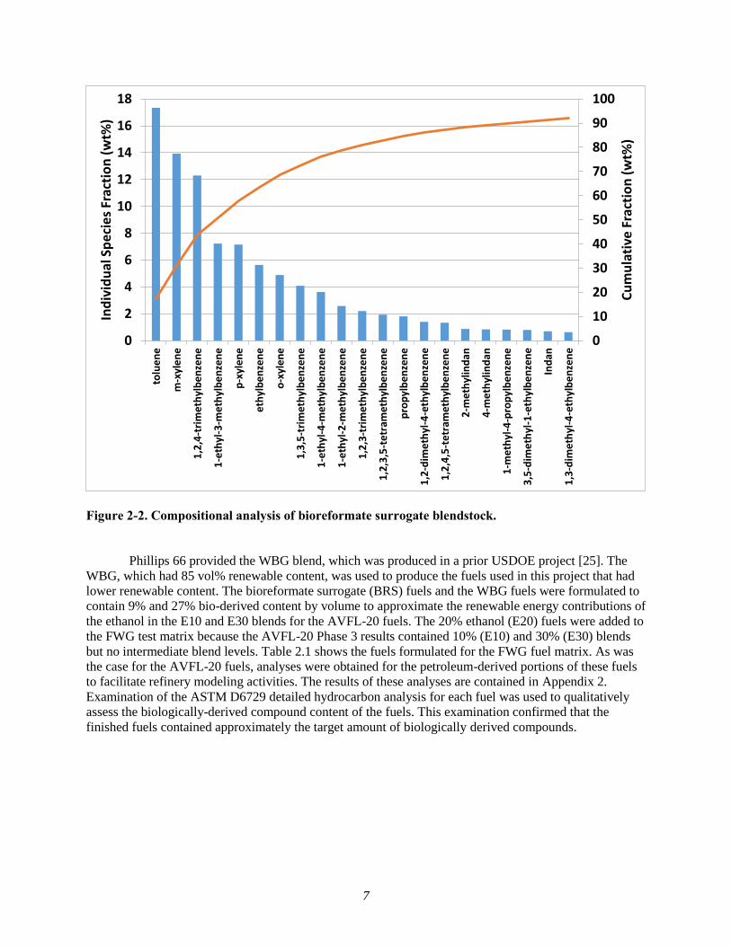
Figure 2-2. Compositional analysis of bioreformate surrogate blendstock.
Phillips 66 provided the WBG blend, which was produced in a prior USDOE project [25]. The
WBG, which had 85 vol% renewable content, was used to produce the fuels used in this project that had
lower renewable content. The bioreformate surrogate (BRS) fuels and the WBG fuels were formulated to
contain 9% and 27% bio-derived content by volume to approximate the renewable energy contributions of
the ethanol in the E10 and E30 blends for the AVFL-20 fuels. The 20% ethanol (E20) fuels were added to
the FWG test matrix because the AVFL-20 Phase 3 results contained 10% (E10) and 30% (E30) blends
but no intermediate blend levels. Table 2.1 shows the fuels formulated for the FWG fuel matrix. As was
the case for the AVFL-20 fuels, analyses were obtained for the petroleum-derived portions of these fuels
to facilitate refinery modeling activities. The results of these analyses are contained in Appendix 2.
Examination of the ASTM D6729 detailed hydrocarbon analysis for each fuel was used to qualitatively
assess the biologically-derived compound content of the fuels. This examination confirmed that the
finished fuels contained approximately the target amount of biologically derived compounds.
0
10
20
30
40
50
60
70
80
90
100
0
2
4
6
8
10
12
14
16
18
tolu
en
e
m-x
yle
ne
1,2
,4-t
rim
eth
ylb
en
zen
e
1-e
thyl
-3-m
eth
ylb
en
zen
e
p-x
yle
ne
eth
ylb
en
zen
e
o-x
yle
ne
1,3
,5-t
rim
eth
ylb
en
zen
e
1-e
thyl
-4-m
eth
ylb
en
zen
e
1-e
thyl
-2-m
eth
ylb
en
zen
e
1,2
,3-t
rim
eth
ylb
en
zen
e
1,2
,3,5
-te
tram
eth
ylb
en
zen
e
pro
pyl
be
nze
ne
1,2
-dim
eth
yl-4
-eth
ylb
en
zen
e
1,2
,4,5
-te
tram
eth
ylb
en
zen
e
2-m
eth
ylin
dan
4-m
eth
ylin
dan
1-m
eth
yl-4
-pro
pyl
be
nze
ne
3,5
-dim
eth
yl-1
-eth
ylb
en
zen
e
Ind
an
1,3
-dim
eth
yl-4
-eth
ylb
en
zen
e
Cu
mu
lati
ve F
ract
ion
(w
t%)
Ind
ivid
ual
Sp
eci
es
Frac
tio
n (
wt%
)

8
Table 2-1. RON, MON, and nominal biologically-derived compound content for the FWG
matrix fuels.
FWG Fuel RON MON Sensitivity
Biofuel Content
(Vol%)
Volumetric
Heating Value
(BTU/Gallon)
CO2 Intensity
(mg CO2/BTU)
#18 101.0 89.0 12.0 20.1 108,358 76.955
#20 97.3 86.6 10.7 20.1 108,736 77.011
BRS1 97.6 87.2 10.4 9.0 116,602 77.660
BRS2 97.3 87.0 10.3 27.0 116,652 78.118
BRS3 101.1 90.0 11.1 9.0 117,738 79.065
BRS4 101.0 90.3 10.7 27.0 118,278 78.570
WBG2 97.7 87.5 10.2 9.0 116,607 78.191
WBG4 97.3 87.1 10.2 27.0 116,663 78.470
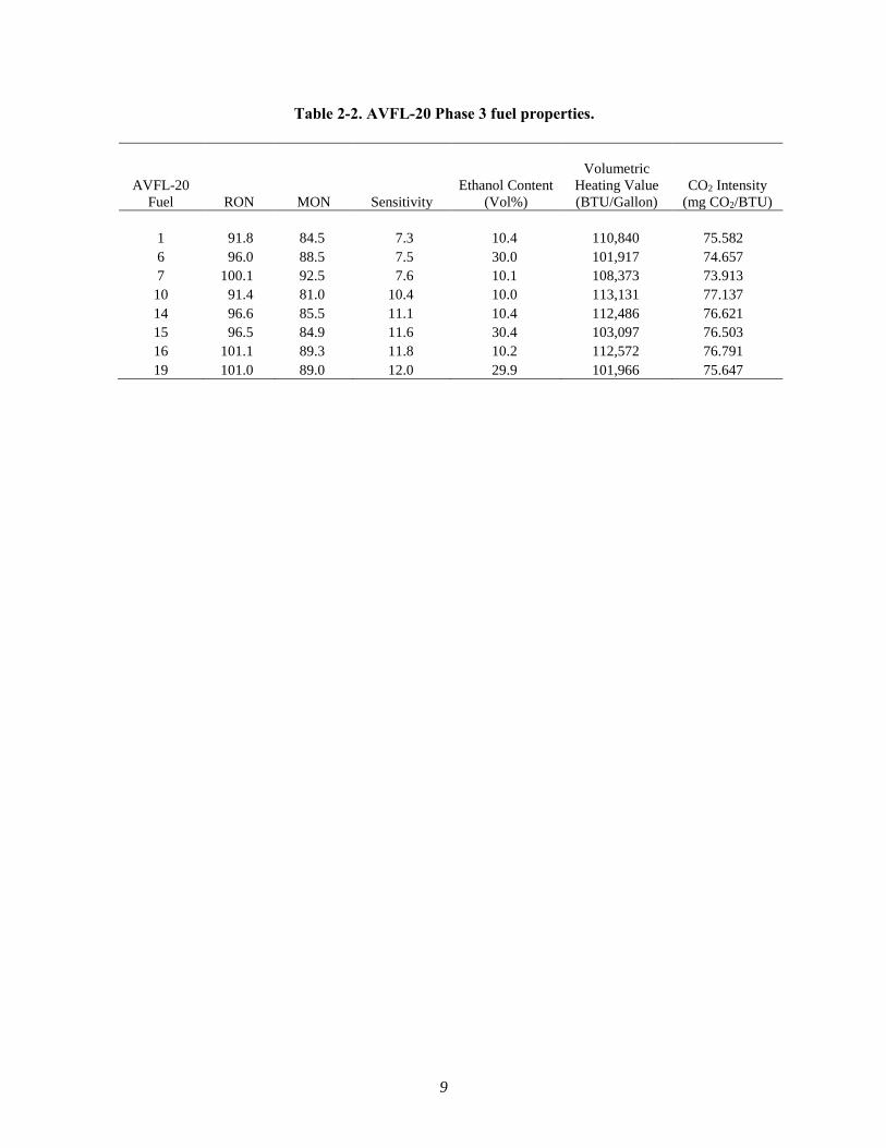
2.2 CRC AVFL-20 Fuels
The CRC AVFL-20 project produced engine fuel consumption maps using fuels with varied
RON, octane sensitivity, and ethanol content [1]. The characteristics of the AVFL-20 Phase 3 fuels are
listed in Table 2.2. Engine fuel consumption maps were produced for six fuels. Similar maps were
anticipated using fuels with ~101 RON, but the nominally CR13:1 pistons intended for use with these
fuels did not provide acceptable combustion performance. In addition, engine failure—unrelated to the
pistons—occurred during the studies with these pistons that required engine replacement. Hence, the
engine mapping and vehicle modeling activities planned for the 101 RON fuels were discontinued.
Additional details for the AVFL-20 fuels are available in the project final report [1]. The U.S.DRIVE
FWG LCA study required information about the characteristics of the petroleum portion of the fuels prior
to ethanol blending in order to support refinery modeling efforts. The petroleum portion of an ethanol-
blended fuel is often referred to as a blendstock for oxygenate blending (BOB), reflecting the fact that the
petroleum portion typically does not meet all of the required properties for a finished fuel, but is designed
to meet all of the required properties once a predetermined amount of ethanol or other oxygenate is added
to it to create the finished fuel. Small volumes of the BOBs for the AVFL-20 fuels were purchased and
analyzed to provide the information needed for refinery modeling efforts, including RON, MON,
volatility-related properties, and hydrocarbon composition. The results of these analyses are included in
Appendix 1.
9
Table 2-2. AVFL-20 Phase 3 fuel properties.
AVFL-20
Fuel RON MON Sensitivity
Ethanol Content
(Vol%)
Volumetric
Heating Value
(BTU/Gallon)
CO2 Intensity
(mg CO2/BTU)
1 91.8 84.5 7.3 10.4 110,840 75.582
6 96.0 88.5 7.5 30.0 101,917 74.657
7 100.1 92.5 7.6 10.1 108,373 73.913
10 91.4 81.0 10.4 10.0 113,131 77.137
14 96.6 85.5 11.1 10.4 112,486 76.621
15 96.5 84.9 11.6 30.4 103,097 76.503
16 101.1 89.3 11.8 10.2 112,572 76.791
19 101.0 89.0 12.0 29.9 101,966 75.647

10
3. Engine Studies
3.1 Engine Hardware and Laboratory Facilities
The hardware and laboratory facilities used to support this work have been reported in detail
previously, but are discussed here briefly [1] [26]. Engine studies were performed at Oak Ridge National
Laboratory (ORNL) using a model year 2013 Ford EcoBoost 1.6-liter, 4-cylinder engine. This engine
incorporates twin-independent cam phasing, center-mount direct fuel injection, and a single-stage
turbocharger. The production pistons nominally produce a CR of 10.1, though subsequent measurements
by ORNL of the hardware used for this project yielded a CR of 10.5. Hereafter, the OEM pistons will be
discussed as having a compression ratio of 10.5. The engine is rated to produce 178 horsepower (HP) at
5,800 revolutions per minute (RPM) and a peak torque of 184 pound-feet (lb-ft) at 2,400 RPM. Vehicles
equipped with this engine are designed to operate using regular grade (87 AKI) gasoline with an ethanol
content of up to 15% by volume. The owner’s manual for the Ford 2013 Escape states that using a
premium grade fuel with this engine will provide improved performance and is recommended for severe
duty, such as trailer tow [27].
In addition to the production pistons, pistons were machined by ORNL from blanks with a
reduced bowl volume to increase the CR [1]. Pistons were produced with CRs of 11.4 and 13.2. A
photograph of the three piston designs is shown in Figure 3-1. Initially, experiments were planned within
this study using both the CR11.4 and CR13.2 pistons. However, as mentioned in the previous section,
ongoing work during the AVFL-20 project found that the CR13.2 pistons did not provide as much
efficiency gain as expected. Computation fluid dynamics (CFD) studies found that the bowl design for
these pistons resulted in delayed and lengthened combustion [1]. In addition, there was an engine failure
in the middle of the CR13.2 studies that damaged the engine and required an engine replacement. As a
result, experiments with these pistons were discontinued for both AVFL-20 and the U.S.DRIVE studies.
Figure 3-1. Photograph of the pistons used for this study.
The engine was controlled using an engine control unit (ECU) provided by Ford Motor Company.
The ECU contained a calibration for the engine that was similar to the calibration used for serial
production, except that some features (such as anti-theft functions, transmission control, traction control)
were disabled to facilitate operation in an engine test cell. Manual adjustments to spark timing were used
OEM CR 11.4 CR 13.2

11
to avoid knock as reported previously. Limitations on CA50, exhaust temperature, and air/fuel ratio were
established based on recommendations provided by staff from Ford Motor Company [1] [26].
A DRIVVEN µDCAT combustion analysis system was used to support the project. (DRIVVEN
has subsequently been purchased by National Instruments, and newer versions of the same software
system and associated hardware modules are now sold through National Instruments Powertrain
Controls.) Combustion analysis is accomplished through high-speed measurement of the pressure in the
combustion cylinders synchronously with the rotation of the crankshaft. Cylinder pressure in each
cylinder was measured using a Kistler 6052CU20 piezoelectric pressure transducer. In combination with
the known (from engine geometric information) volume of the combustion cylinders at each crankshaft
rotation position, these data can be used to evaluate the combustion process.
For this project, the cylinder #1 pressure signal was split to both a synchronous measurement
channel (for combustion characterization) and a high-speed asynchronous channel (for knock detection).
The high-speed asynchronous channel sampled the pressure in cylinder #1 on a time basis, rather than on
a crank-angle basis, so that high-frequency oscillation in the pressure can be measured. The time-based
measurement as used to supply a signal for knock detection within the µDCAT software. The ECU anti-
knock features were disabled during this study in order to allow the operator to manually control spark
timing to avoid knock based on feedback from the µDCAT knock detection algorithms. Further details
are available in the CRC AVFL-20 project report [1].
The engine was installed in an engine research facility using an alternating current dynamometer
to absorb the output torque of the engine. Temperature and humidity-controlled air was provided to the
engine air intake. The air supply temperature was maintained at 75 °F, with a dew point of 58 °F. Fuel
consumption was measured using a Micro-motion Coriolis mass flow meter. Other standard laboratory
instrumentation for measuring pressures, temperatures, and so on were also used.
3.2 Engine Study Results for FWG Fuel Matrix
The nominal 97 RON fuels in the FWG fuel matrix were studied using the CR11.4 pistons.
Experiments for the present study were conducted in accordance with methods used and previously
reported for the AVFL-20 study. Engine fuel consumption maps were developed by collecting data at
engine speeds of 1,000; 1,500; 2,000; 2,500; and 5,000 RPM, capturing the full range of engine torque
output. Additionally, maximum torque points were collected at 3,000–4,500 RPM. Although studies with
the 101 RON fuels in the FWG matrix were originally planned, these studies were discontinued because
of performance issues with the CR13.2 pistons that were discovered during the AVFL-20 project plus an
engine failure not related to the pistons that required an engine replacement [1]. Figure 3-2 shows the
engine speed and brake mean effective pressure (BMEP) points for fuel #20 using CR11.4, and is typical
of the range of conditions used to measure the fuel consumption for all of the study fuels.
3.2.1 Combustion Phasing Results
A common metric for describing the phasing of the combustion event relative to the crankshaft
position is the crank angle position at which 50% of the fuel mass has burned, or CA50. CA50 is
measured in crank angle degrees (CAD) after top-dead-center (ATDC). BMEP is a metric that describes
the torque output of the engine per cycle per unit of displacement. BMEP is frequently measured in
kilopascals (kPa). BMEP is a useful metric because it allows results and trends from engines of differing
displacement to be compared directly with one another. Figure 3-3 shows the combustion phasing results
for the 5 FWG matrix fuels at an engine speed of 2,000 RPM. The trends for all five fuels show nearly
constant combustion phasing in the maximum brake torque (MBT) region where knock does not occur.
As the engine encounters knock, combustion phasing is retarded to avoid the knocking condition. The

12
results for the four ethanol-free fuels are similar, which is expected given their relatively tightly-
controlled RON and sensitivity values. The E20 fuel required slightly less retarded combustion phasing
for several conditions at 2,000 RPM. CA50 results at other engine speeds showed similar trends and less
difference between the E20 and ethanol-free fuels.
Figure 3-2. Engine speed and BMEP conditions included in the engine map for
fuel #20 at CR11.4.
0
500
1000
1500
2000
2500
0 1000 2000 3000 4000 5000 6000
Bra
ke M
ean
Eff
ect
ive
Pre
ssu
re (
kPa)
Engine Speed (RPM)

13
Figure 3-3. Combustion phasing results for the 97 RON FWG matrix fuels at
2,000 RPM with the CR11.4 pistons.
3.2.2 Fuel Mean Effective Pressure Results
Fuel mean effective pressure, or fuel MEP, is a metric that describes the fuel energy consumption
of the engine per cycle per unit of displacement. As with BMEP, fuel MEP is reported in units of
pressure, kPa. In the MBT region, fuel MEP is linearly proportional to BMEP and is not very sensitive to
engine speed [28] [29] [30]. Fuel MEP results in the MBT region for the five 97 RON fuels are shown in
Figure 3.3. The results for all five fuels fall onto one line, indicating low scatter or “noise” in the collected
engine data and self-consistency between the engine data and the heating value analyses for all of the
fuels. The regression results shown in Figure 3.4 were developed using data in the MBT region at engine
speeds between 1,500 and 2,500 RPM and were used to calculate the fuel consumption rates within the
MBT region for all of the fuels. This approach offers the advantage of minimizing the impact of
experimental noise in the MBT region on modeled fuel economy predictions. The measured fuel
consumption values for each fuel were used for conditions in the knock-limited region. The same
approach was used in the AVFL-20 project.
The fuel MEP correlation for the FWG fuel matrix, as shown in Figure 3.4, had a slope of 2.4685
and an intercept of 416.89. The correlation determined for the AVFL-20 fuel set at CR11.4 had a slope of
2.4314 and an intercept of 417.56 [1]. These differences result in different fuel consumption values for
the two fuel matrices, with the AVFL-20 fuels demonstrating marginally higher efficiency in the MBT
space. Fuel MEP values for the FWG matrix fuel #20 (an E20 blend) were directionally more similar to
the AVFL-20 results than the ethanol-free fuels. These observations suggest that fuel formulation may
contribute to the difference in the fuel MEP regressions in the MBT space. For example, part-load
benefits from ethanol blending that could explain the differences noted in this study have been reported
0
5
10
15
20
25
30
35
0 500 1000 1500 2000 2500
Cyl
ind
er
#1 C
A5
0 (
CA
D A
TDC
)
Brake Mean Effective Pressure (kPa)
#20BRS1BRS2WBG2WBG4
Fuel RON Sensitivity
Bio-Content
(Vol%)
#20 97.3 10.1 20
BRS1 97.3 9.9 9
BRS2 97.1 9.8 27
WBG2 97.6 9.3 9
WBG4 97.6 9.4 27
On
set
of
Kn
ock

14
previously [31]. The differences in the fuel MEP correlations result in a difference in engine brake
thermal efficiency of up to 0.4 engine efficiency points in the MBT region.
Figure 3-4. Fuel MEP for the five 97 RON fuels in the MBT region at engine
speeds 1,500–2,500 RPM.
y = 2.4685x + 416.89R² = 0.9992
0
500
1000
1500
2000
2500
3000
0 200 400 600 800 1000
Fue
l Me
an E
ffe
ctiv
e P
ress
ure
(kP
a)
Brake Mean Effective Pressure (kPa)
Fuel RON Sensitivity
Bio-Content
(Vol%)
#20 97.3 10.1 20
BRS1 97.3 9.9 9
BRS2 97.1 9.8 27
WBG2 97.6 9.3 9
WBG4 97.6 9.4 27

15
4. Vehicle Modeling
Vehicle modeling allows the engine data gathered during this project to be used to estimate the
energy consumption, volumetric fuel economy, and tailpipe CO2 emissions from vehicles that might use
engines with the different CRs and fuels studied in this project. This study adopted the vehicle models
used for AVFL-20 to assure compatibility of results from the two projects. The Autonomie vehicle
simulation software package was used to develop models for a mid-size sedan and a small SUV [1].
Autonomie has been extensively benchmarked, and offers the advantage of being a non-proprietary
modeling tool designed to assess fuel consumption for conventional and hybrid vehicle designs
[2][3][4][5]. The drive cycles studied include the urban dynamometer driving schedule (UDDS), the
highway fuel economy test (HWFET), and the US06 cycle. Results for the US06 cycle were divided into
results for both the city and highway portions of the cycle.
4.1 Parameters Describing the Model Vehicles
Several parameters are needed in vehicle simulation models to describe the aerodynamic and
inertial loads placed on the vehicle and its powertrain during operation. Aerodynamic and inertial loads at
the tire/road interface are specified by the dynamometer target coefficients and equivalent test weight that
are available in the EPA certification test database for all vehicles sold in the United States [32]. The
forces at the tire are translated to forces at the engine output shaft through the differential and
transmission. Hence, the relevant gear ratios and final drive ratio also need to be specified. The AVFL-20
report contains details of the data-mining process that was used to determine the parameters used to
describe the mid-size sedan and small SUV [1]. This study adopted the same parameters that were
selected for AVFL-20. These parameters are summarized in Table 4.1.
Table 4-1. Parameters used in the Autonomie model for the
midsize sedan and small SUV.
Parameter
Mid-Size
Sedan Small SUV
Target Coefficient A (lbf) 34.0501 31.3622
Target Coefficient B (lbf/MPH) 0.2061 0.3408
Target Coefficient C (lbf/MPH^2) 0.0178 0.0235
Engineering Test Weight (lbs) 4000 4000
1st Gear Ratio 3.73 4.584
2nd Gear Ratio 2.05 2.964
3rd Gear Ratio 1.36 1.912
4th Gear Ratio 1.03 1.446
5th Gear Ratio 0.82 1.000
6th Gear Ratio 0.69 0.746
Final Drive Ratio 4.07 3.21
Tire Rolling Radius (m) 0.32775 0.32775

16
4.2 Vehicle Model Results
The vehicle model provides a means of comparing the potential impacts of fuel and CR, but is
subject to some limitations. Specifically, steady-state engine maps are used to provide fuel consumption
information to the model. These steady-state maps do not provide a reliable means of examining the
important impacts from cold-start, for example. Furthermore, steady-state conditions in an engine
research laboratory can result in hotter conditions during the combustion process than occur in transient
excursions at high BMEP levels. These differences between the model environment and on-road
operation are significant, however, this approach remains useful for comparing the potential impacts of
fuel formulations and compression ratio, since the modeled conditions are consistent among the fuels and
compression ratios being studied.
4.2.1 Results for the FWG Matrix Fuels using CR11.4 Pistons
Vehicle energy consumption over a drive cycle is a metric that provides insight into directional
changes in engine efficiency afforded by different fuels and compression ratios. Figures 4-1 and 4-2 show
the energy consumption for the mid-size sedan and small SUV, respectively, using the CR11.4 pistons.
The results show that differences from the maximum to minimum value on a given cycle vary between
0.4% to 2.3% for the sedan and 0.9% to 3.1% for the SUV. The similarity in results is expected, given
that the fuels had very similar RON and sensitivity, and were tested at the same CR.
Volumetric fuel economy depends both on the vehicle energy consumption for a given cycle and
on the volumetric heating value of the fuel. Figure 4.3 shows the volumetric heating value for each fuel.
There is little variation in the volumetric heating value of the ethanol-free fuels, but the E20 blend has a
heating value that is 6.7% lower than the BRS1 fuel, for example. In order for the E20 fuel to achieve a
higher volumetric fuel economy than the other fuels, it would need to offset at least 6.7% energy
consumption on a given drive cycle. Thus, the volumetric fuel economy for the E20 fuel is lower relative
to the other 97 RON fuels at this CR, as shown in Figures 4.4 and 4.5, despite slightly lower energy
consumption for this fuel as noted above. Compared to WBG4, the E20 fuel has about 7% poorer (lower)
fuel economy on the UDDS and HWFET drive cycle for both the sedan and SUV and 4.7%–6.7% poorer
(lower) fuel economy on the US06 drive cycles. Differences among the volumetric fuel economy values
for the non-ethanol fuels were small relative to the difference between these fuels and the E20 fuel,
consistent with their volumetric heating values. These trends were observed for both the mid-size sedan
and small SUV.
Tailpipe CO2 emissions for a given drive cycle depend on both the vehicle energy consumption
for the cycle and the carbon intensity of the fuel. In this case, the carbon intensity is defined as the mass
of tailpipe CO2 emitted per unit fuel energy combusted (BTU) and should not be confused with the CO2
required to produce the fuel. Figure 4.6 shows the carbon intensity of the FWG matrix fuels studied at
CR11.4, as the fuels were produced for the engine study.

17
Figure 4-1. Modeled energy consumption results for the mid-size sedan using the
FWG matrix fuels and the CR11.4 pistons.
Figure 4-2. Modeled energy consumption results for the small SUV using the
FWG matrix fuels and CR11.4 pistons.
3,7
52
2,6
32
7,2
11
3,6
65
3,8
19
2,6
44
7,4
17
3,7
06
3,7
75
2,6
42
7,3
83
3,7
16
3,7
68
2,6
40
7,2
83
3,6
87
3,7
55
2,6
36
7,2
78
3,6
81
0
1000
2000
3000
4000
5000
6000
7000
8000
9000
10000
UDDS HWFET US06_CITY US06_HWY
Ene
rgy
Co
nsu
mp
tio
n (
BTU
/Mile
)
Fuel RON Sensitivity
Bio-Content
(Vol%)
#20 97.3 10.1 20
BRS1 97.3 9.9 9
BRS2 97.1 9.8 27
WBG2 97.6 9.3 9
WBG4 97.6 9.4 27
3,8
10
2,8
80
7,2
49
4,0
57
3,8
84
2,9
06
7,4
79
4,1
35
3,8
36
2,9
07
7,4
68
4,1
34
3,8
29
2,9
03
7,3
76
4,1
26
3,8
18
2,8
91
7,4
12
4,0
88
0
1000
2000
3000
4000
5000
6000
7000
8000
9000
10000
UDDS HWFET US06_CITY US06_HWY
Ene
rgy
Co
nsu
mp
tio
n (
BTU
/Mile
)
Fuel RON Sensitivity
Bio-Content
(Vol%)
#20 97.3 10.1 20
BRS1 97.3 9.9 9
BRS2 97.1 9.8 27
WBG2 97.6 9.3 9
WBG4 97.6 9.4 27

18
Figure 4-3. Volumetric heating value for the FWG matrix fuels studied at CR11.4.
Figure 4-4. Modeled volumetric fuel economy for the mid-size sedan using the 97
RON FWG matrix fuels and CR11.4 pistons.
10
8,7
36
11
6,6
02
11
6,6
52
11
6,6
07
11
6,6
63
0
20000
40000
60000
80000
100000
120000
140000
#20 BRS1 BRS2 WBG2 WBG4
Vo
lum
etr
ic H
eat
ing
Val
ue
(B
TU/g
allo
n)
29
.0
41
.3
15
.1
29
.7
30
.5
44
.1
15
.7
31
.5
30
.9
44
.2
15
.8
31
.4
31
.0
44
.2
16
.0
31
.6
31
.1
44
.3
16
.0
31
.7
0
5
10
15
20
25
30
35
40
45
50
UDDS HWFET US06_CITY US06_HWY
Vo
lum
etr
ic F
ue
l Eco
no
my
(Mile
s/G
allo
n)
Fuel RON Sensitivity
Bio-Content
(Vol%)
#20 97.3 10.1 20
BRS1 97.3 9.9 9
BRS2 97.1 9.8 27
WBG2 97.6 9.3 9
WBG4 97.6 9.4 27

19
Figure 4-5. Modeled fuel economy for the small SUV using the 97 RON FWG
matrix fuels and CR11.4 pistons.
Figure 4-6. CO2 intensity for the 97 RON FWG matrix fuels.
28
.5
37
.8
15
.0
26
.8
30
.0
40
.1
15
.6
28
.230
.4
40
.1
15
.6
28
.230
.5
40
.2
15
.8
28
.330
.6
40
.4
15
.7
28
.5
0
5
10
15
20
25
30
35
40
45
UDDS HWFET US06_CITY US06_HWY
Vo
lum
etr
ic F
ue
l Eco
no
my
(Mile
s/G
allo
n)
Fuel RON Sensitivity
Bio-Content
(Vol%)
#20 97.3 10.1 20
BRS1 97.3 9.9 9
BRS2 97.1 9.8 27
WBG2 97.6 9.3 9
WBG4 97.6 9.4 27
77
.01
1
77
.66
1
78
.11
8
78
.19
1
78
.47
0
0
10
20
30
40
50
60
70
80
90
#20 BRS1 BRS2 WBG2 WBG4
CO
2In
ten
sity
(m
g C
O2
/ B
TU)

20
Figures 4-7 and 4-8 show the modeled tailpipe CO2 emissions for the mid-size sedan and small
SUV, respectively. These values are based on the total carbon content of each fuel, and are thus the total
of both biogenic and petroleum-derived tailpipe CO2 emissions. In all cases, the largest tailpipe CO2
emissions were observed for either BRS1 or BRS2, though the marginal difference between these fuels
and the other ethanol-free fuels is probably not significant. The E20 fuel provided the lowest overall
tailpipe CO2 emissions. The difference between maximum and minimum values of tailpipe CO2 emissions
among these fuels ranged from 2.0% to 3.7% for the sedan and from 2.3% to 4.3% for the SUV over the
four cycles. Table 4-2 summarizes the modeled energy use, volumetric fuel economy, and tailpipe CO2
emissions for the FWG fuels.
Figure 4-7. Modeled tailpipe CO2 emissions for the mid-size sedan using the
FWG matrix fuels and CR11.4 pistons.
28
9
20
3
55
5
28
2
29
7
20
5
57
6
28
8
29
5
20
6
57
7
29
0
29
5
20
6
56
9
28
8
29
5
20
7
57
1
28
90
100
200
300
400
500
600
700
UDDS HWFET US06_CITY US06_HWY
Tailp
ipe
CO
2Em
issi
on
s (g
/mile
)
Fuel RON Sensitivity
Bio-Content
(Vol%)
#20 97.3 10.1 20
BRS1 97.3 9.9 9
BRS2 97.1 9.8 27
WBG2 97.6 9.3 9
WBG4 97.6 9.4 27

21
Figure 4-8. Modeled tailpipe CO2 emissions for the small SUV using the FWG
matrix fuels and CR11.4 pistons.
Table 4-2. Summary of vehicle model results for the mid-size sedan and small SUV using
FWG 97 RON fuels and CR11.4.
29
3
22
2
55
8
31
2
30
2
22
6
58
1
32
1
30
0
22
7
58
3
32
3
29
9
22
7
57
7
32
3
30
0
22
7
58
2
32
1
0
100
200
300
400
500
600
700
UDDS HWFET US06_CITY US06_HWY
Tailp
ipe
CO
2Em
issi
on
s (g
/mile
)
Fuel RON Sensitivity
Bio-Content
(Vol%)
#20 97.3 10.1 20
BRS1 97.3 9.9 9
BRS2 97.1 9.8 27
WBG2 97.6 9.3 9
WBG4 97.6 9.4 27
Drive
Cycle Sedan SUV Sedan SUV Sedan SUV Sedan SUV Sedan SUV
UDDS 3,752 3,810 3,819 3,884 3,775 3,836 3,768 3,829 3755 3818
HWFET 2,632 2,880 2,644 2,906 2,642 2,907 2,640 2,903 2636 2891
US06 City 7,211 7,249 7,417 7,479 7,383 7,468 7,283 7,376 7278 7412
US06 Hwy 3,665 4,057 3,706 4,135 3,716 4,134 3,687 4,126 3681 4088
UDDS 29.0 28.5 30.5 30.0 30.9 30.4 31.0 30.5 31.1 30.6
HWFET 41.3 37.8 44.1 40.1 44.2 40.1 44.2 40.2 44.3 40.4
US06 City 15.1 15.0 15.7 15.6 15.8 15.6 16.0 15.8 16 15.7
US06 Hwy 29.7 26.8 31.5 28.2 31.4 28.2 31.6 28.3 31.7 28.5
UDDS 289 293 297 302 295 300 295 299 295 300
HWFET 203 222 205 226 206 227 206 227 207 227
US06 City 555 558 576 581 577 583 569 577 571 582
US06 Hwy 282 312 288 321 290 323 288 323 289 321
97.6 RON, 9.3 S, 9% Bio
Energy
Consumption
(BTU/Mile)
Volumetric
Fuel Economy
(MPG)
Tailpipe CO2
Emissions
(g/mile)
Vehicle model results for the mid-size sedan and small SUV for CR11.4
WBG497.6 RON, 9.4 S, 27% Bio
Fuel #20 BRS1 BRS2 WBG2
97.3 RON, 10.1 S, E20 97.3 RON, 9.9 S, 9% Bio 97.1 RON, 9.8 S, 27% Bio
22
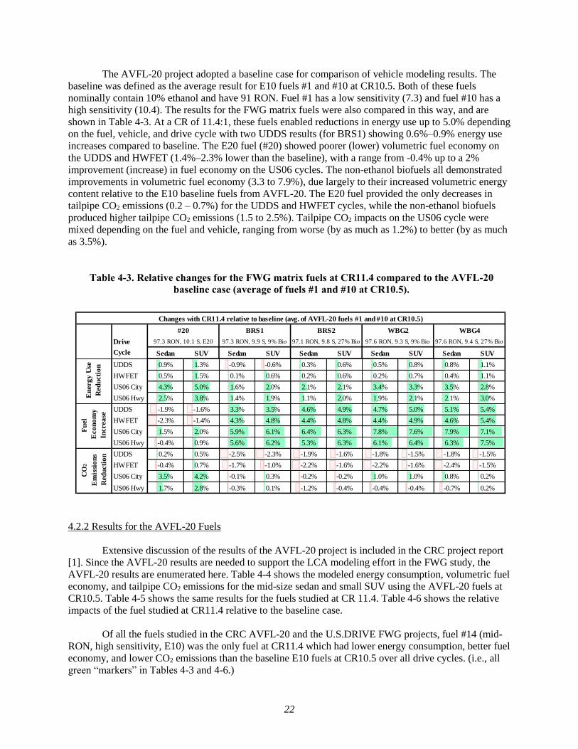
The AVFL-20 project adopted a baseline case for comparison of vehicle modeling results. The
baseline was defined as the average result for E10 fuels #1 and #10 at CR10.5. Both of these fuels
nominally contain 10% ethanol and have 91 RON. Fuel #1 has a low sensitivity (7.3) and fuel #10 has a
high sensitivity (10.4). The results for the FWG matrix fuels were also compared in this way, and are
shown in Table 4-3. At a CR of 11.4:1, these fuels enabled reductions in energy use up to 5.0% depending
on the fuel, vehicle, and drive cycle with two UDDS results (for BRS1) showing 0.6%–0.9% energy use
increases compared to baseline. The E20 fuel (#20) showed poorer (lower) volumetric fuel economy on
the UDDS and HWFET (1.4%–2.3% lower than the baseline), with a range from -0.4% up to a 2%
improvement (increase) in fuel economy on the US06 cycles. The non-ethanol biofuels all demonstrated
improvements in volumetric fuel economy (3.3 to 7.9%), due largely to their increased volumetric energy
content relative to the E10 baseline fuels from AVFL-20. The E20 fuel provided the only decreases in
tailpipe CO2 emissions (0.2 – 0.7%) for the UDDS and HWFET cycles, while the non-ethanol biofuels
produced higher tailpipe CO2 emissions (1.5 to 2.5%). Tailpipe CO2 impacts on the US06 cycle were
mixed depending on the fuel and vehicle, ranging from worse (by as much as 1.2%) to better (by as much
as 3.5%).
Table 4-3. Relative changes for the FWG matrix fuels at CR11.4 compared to the AVFL-20
baseline case (average of fuels #1 and #10 at CR10.5).
4.2.2 Results for the AVFL-20 Fuels
Extensive discussion of the results of the AVFL-20 project is included in the CRC project report
[1]. Since the AVFL-20 results are needed to support the LCA modeling effort in the FWG study, the
AVFL-20 results are enumerated here. Table 4-4 shows the modeled energy consumption, volumetric fuel
economy, and tailpipe CO2 emissions for the mid-size sedan and small SUV using the AVFL-20 fuels at
CR10.5. Table 4-5 shows the same results for the fuels studied at CR 11.4. Table 4-6 shows the relative
impacts of the fuel studied at CR11.4 relative to the baseline case.
Of all the fuels studied in the CRC AVFL-20 and the U.S.DRIVE FWG projects, fuel #14 (mid-
RON, high sensitivity, E10) was the only fuel at CR11.4 which had lower energy consumption, better fuel
economy, and lower CO2 emissions than the baseline E10 fuels at CR10.5 over all drive cycles. (i.e., all
green “markers” in Tables 4-3 and 4-6.)
Drive
Cycle Sedan SUV Sedan SUV Sedan SUV Sedan SUV Sedan SUV
UDDS 0.9% 1.3% -0.9% -0.6% 0.3% 0.6% 0.5% 0.8% 0.8% 1.1%
HWFET 0.5% 1.5% 0.1% 0.6% 0.2% 0.6% 0.2% 0.7% 0.4% 1.1%
US06 City 4.3% 5.0% 1.6% 2.0% 2.1% 2.1% 3.4% 3.3% 3.5% 2.8%
US06 Hwy 2.5% 3.8% 1.4% 1.9% 1.1% 2.0% 1.9% 2.1% 2.1% 3.0%
UDDS -1.9% -1.6% 3.3% 3.5% 4.6% 4.9% 4.7% 5.0% 5.1% 5.4%
HWFET -2.3% -1.4% 4.3% 4.8% 4.4% 4.8% 4.4% 4.9% 4.6% 5.4%
US06 City 1.5% 2.0% 5.9% 6.1% 6.4% 6.3% 7.8% 7.6% 7.9% 7.1%
US06 Hwy -0.4% 0.9% 5.6% 6.2% 5.3% 6.3% 6.1% 6.4% 6.3% 7.5%
UDDS 0.2% 0.5% -2.5% -2.3% -1.9% -1.6% -1.8% -1.5% -1.8% -1.5%
HWFET -0.4% 0.7% -1.7% -1.0% -2.2% -1.6% -2.2% -1.6% -2.4% -1.5%
US06 City 3.5% 4.2% -0.1% 0.3% -0.2% -0.2% 1.0% 1.0% 0.8% 0.2%
US06 Hwy 1.7% 2.8% -0.3% 0.1% -1.2% -0.4% -0.4% -0.4% -0.7% 0.2%
En
erg
y U
se
Red
ucti
on
Fu
el
Eco
no
my
Increa
se
CO
2
Em
issi
on
s
Red
ucti
on
WBG4
97.6 RON, 9.4 S, 27% Bio
Changes with CR11.4 relative to baseline (avg. of AVFL-20 fuels #1 and #10 at CR10.5)
#20 BRS1 BRS2 WBG2
97.3 RON, 10.1 S, E20 97.3 RON, 9.9 S, 9% Bio 97.1 RON, 9.8 S, 27% Bio 97.6 RON, 9.3 S, 9% Bio

23
Table 4-4. Vehicle model results for the mid-size sedan and small SUV using
the CR10.5 pistons and fuels studied in AVFL-20. [1]
Table 4-5. Vehicle model results for the mid-size sedan and small SUV using the CR11.4
pistons and fuels studied in AVFL-20 [1].
Drive
Cycle Sedan SUV Sedan SUV Sedan SUV
UDDS 3,765 3,838 3,808 3,884 3,729 3,799
HWFET 2,643 2,918 2,650 2,929 2,633 2,897
US06 City 7,494 7,561 7,582 7,696 6,943 7,100
US06 Hwy 3,756 4,200 3,761 4,232 3,633 4,001
UDDS 29.4 28.9 29.7 29.1 27.7 27.1
HWFET 41.9 38.0 42.7 38.6 39.2 35.6
US06 City 14.8 14.7 14.9 14.7 14.9 14.5
US06 Hwy 29.5 26.4 30.1 26.7 28.4 25.8
UDDS 285 290 294 300 285 291
HWFET 200 221 204 226 201 222
US06 City 566 571 585 594 531 543
US06 Hwy 284 317 290 326 278 306
91 RON, 10 S, E10 97 RON, 12 S, E30
Energy
Consumption
(BTU/Mile)
Volumetric Fuel
Economy (MPG)
Tailpipe CO2
Emissions
(g/mile)
Vehicle model results for the mid-size sedan and small SUV for CR10.5
Fuel #1 Fuel #10 Fuel #15
92 RON, 7 S, E10
Drive
Cycle Sedan SUV Sedan SUV Sedan SUV Sedan SUV
UDDS 3,720 3,787 3,728 3,789 3,745 3,813 3,717 3,782
HWFET 2,605 2,863 2,610 2,860 2,621 2,882 2,609 2,859
US06 City 7,254 7,322 7,225 7,259 7,309 7,381 7,086 7,230
US06 Hwy 3,644 4,060 3,634 4,042 3,664 4,092 3,616 3,988
UDDS 27.4 26.9 29.1 28.6 30.0 29.5 27.7 27.3
HWFET 39.1 35.6 41.5 37.9 42.9 39.0 39.5 36.1
US06 City 14.1 13.9 15.0 14.9 15.4 15.2 14.6 14.3
US06 Hwy 28.0 25.1 29.8 26.8 30.7 27.5 28.5 25.9
UDDS 278 283 276 280 287 292 284 289
HWFET 194 214 193 211 201 221 200 219
US06 City 542 547 534 537 560 566 542 553
US06 Hwy 272 303 269 299 281 314 277 305
Tailpipe CO2
Emissions
(g/mile)
96 RON, 8 S, E30 100 RON, 8 S, E10 97 RON, 11 S, E10 97 RON, 12 S, E30
Energy
Consumption
(BTU/Mile)
Vehicle model results for the mid-size sedan and small SUV for CR11.4
Fuel #6 Fuel #7 Fuel #14 Fuel #15
Volumetric Fuel
Economy (MPG)

24
Table 4-6. Impacts of AVFL-20 fuels studied at CR11.4 relative to the baseline case (average
of fuels #1 and #10 at CR10.5) [1].
Drive
Cycle Sedan SUV Sedan SUV Sedan SUV Sedan SUV
UDDS 1.8% 1.9% 1.5% 1.9% 1.1% 1.2% 1.8% 2.0%
HWFET 1.6% 2.1% 1.4% 2.2% 1.0% 1.4% 1.4% 2.2%
US06 City 3.8% 4.0% 4.2% 4.8% 3.0% 3.2% 6.0% 5.2%
US06 Hwy 3.1% 3.7% 3.3% 4.1% 2.5% 2.9% 3.8% 5.4%
UDDS -7.4% -7.2% -1.7% -1.4% 1.6% 1.7% -6.2% -6.0%
HWFET -7.5% -7.0% -1.9% -1.1% 1.4% 1.9% -6.6% -5.8%
US06 City -5.4% -5.2% 1.0% 1.7% 3.6% 3.8% -2.1% -2.9%
US06 Hwy -6.1% -5.5% 0.0% 0.9% 3.0% 3.5% -4.3% -2.7%
UDDS 4.0% 4.1% 4.7% 5.0% 0.8% 0.9% 1.7% 1.9%
HWFET 3.8% 4.3% 4.5% 5.3% 0.6% 1.1% 1.3% 2.0%
US06 City 5.9% 6.2% 7.2% 7.9% 2.7% 2.9% 5.8% 5.1%
US06 Hwy 5.2% 5.8% 6.4% 7.2% 2.2% 2.6% 3.6% 5.2%
CO
2
Em
issi
on
s
Red
ucti
on
Fu
el
Eco
no
my
Increa
se
En
erg
y U
se
Red
ucti
on
97 RON, 12 S, E30
Changes with CR11.4 relative to baseline (avg. of fuels #1 and #10 at CR10.5)
Fuel #15
96 RON, 8 S, E30 100 RON, 8 S, E10
Fuel #7 Fuel #14Fuel #6
97 RON, 11 S, E10

25
5. Vehicle Characteristics to Support LCA Modeling
The engine and vehicle modeling study outlined previously was used in combination with other
published results to establish energy consumption metrics that represent the light-duty U.S. fleet. This
section outlines the process used to cascade the vehicle model results into the inputs needed to support
LCA for the study fuels. Although the measured fuel properties of the study fuels in general compared
favorably with target values, small deviations are an unavoidable part of experimental studies. The actual
compression ratio enabled by each fuel therefore differs slightly from the fixed compression ratios that
were used in the engine studies. The vehicle efficiency gain for each fuel was estimated through a multi-
step process that is outlined in the following sections of the report. This process provided a consistent
means of estimating the benefits that may be enabled by both the 97 RON and 101 RON fuels.
5.1 Compression Ratio Increase Enabled by Each Fuel
The combustion phasing screening results at 2,000 RPM from the AVFL-20 and FWG engine
studies showed that the 97 RON fuels in both matrices enabled CR 11.4 and also that the 101 RON fuels
enabled CR 13.2. Results from the 97 RON fuels at CR 11.4, compared with the 91 RON fuels at the
baseline CR 10.5, show that 5.6 octane numbers (ON) are needed per unit CR increase. Similarly, the 101
RON fuels at CR 13.2 show that 3.7 ON are needed per CR increase. Two previously-published studies
also investigated the ON/CR relationship in modern engines. The first of these studies, conducted at the
University of Birmingham in the United Kingdom, summarized the CR improvements enabled by high-
octane fuels in multiple studies at multiple research organizations. The ON/CR values ranged from 2.4 to
5.0, with a mean value of 3.9 and a median of 3.5 [33]. The second study was conducted by the member
companies of USCAR. It also reported ON/CR values, ranging from 2.5 to just over 9.0 [6]. Typically,
studies that investigate benefits from increasing CR use a well-optimized production engine as a baseline
case and increase CR through piston replacement using pistons that are less optimized. Thus, it is possible
that engines developed by the automotive manufacturers using increased CR will require lower values of
ON/CR compared with existing studies. The range of values for ON/CR suggests that multiple values be
studied to capture the potential breadth of the effect of increasing octane rating on vehicle fuel efficiency.
The AVFL-20 and FWG result of 5.6 ON/CR was selected for study, as it is a reasonable representation
of the upper end of the ON/CR range (though it is not the maximum value). Similarly, the 3.7 ON/CR
result from the AVFL-20 study was also selected, as it is similar to the mean and median values of the
ON/CR results enumerated in the University of Birmingham study and USCAR studies. Finally, a value
of 3.0 ON/CR was selected to represent the ON requirements for more fully-optimized engines that could
potentially be developed by the automakers, and it represents the lower end of the reported ON/CR range
(though it is not the minimum value). Table 5-1 shows the CR levels that are projected to be enabled for
each fuel at the three ON/CR levels studied.
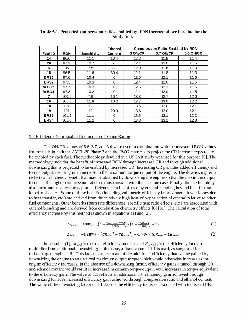
26
Table 5-1. Projected compression ratios enabled by RON increase above baseline for the
study fuels.
5.2 Efficiency Gain Enabled by Increased Octane Rating
The ON/CR values of 5.6, 3.7, and 3.0 were used in combination with the measured RON values
for the fuels in both the AVFL-20 Phase 3 and the FWG matrices to project the CR increase expected to
be enabled by each fuel. The methodology detailed in a USCAR study was used for this purpose [6]. The
methodology includes the benefit of increased RON through increased CR and through additional
downsizing that is projected to be enabled by increased CR. Increasing CR provides added efficiency and
torque output, resulting in an increase in the maximum torque output of the engine. The downsizing term
reflects an efficiency benefit that may be obtained by downsizing the engine so that the maximum output
torque at the higher compression ratio remains constant with the baseline case. Finally, the methodology
also incorporates a term to capture efficiency benefits offered by ethanol blending beyond its effect on
knock resistance. Some of these benefits (including volumetric efficiency improvement, lower losses due
to heat transfer, etc.) are derived from the relatively high heat-of-vaporization of ethanol relative to other
fuel components. Other benefits (burn rate differences, specific heat ratio effects, etc.) are associated with
ethanol blending and are derived from combustion chemistry effects [6] [31]. The calculation of total
efficiency increase by this method is shown in equations (1) and (2).
∆𝝐𝒕𝒐𝒕𝒂𝒍 = 𝟏𝟎𝟎% ∗ ((𝟏 +𝑭𝒅𝒐𝒘𝒏𝒔𝒊𝒛𝒆∗ ∆𝝐𝑪𝑹
𝟏𝟎𝟎%) ∗ (𝟏 +
∆𝝐𝒆𝒕𝒉𝒂𝒏𝒐𝒍
𝟏𝟎𝟎%) − 𝟏) (1)
∆𝝐𝑪𝑹 = −𝟎. 𝟐𝟎𝟕% ∗ (𝑪𝑹𝒏𝒆𝒘𝟐 − 𝑪𝑹𝒃𝒂𝒔𝒆
𝟐) + 𝟔. 𝟒𝟒% ∗ (𝑪𝑹𝒏𝒆𝒘 − 𝑪𝑹𝒃𝒂𝒔𝒆) (2)
In equation (1), Δεtotal is the total efficiency increase and Fdownsize is the efficiency increase
multiplier from additional downsizing; in this case, a fixed value of 1.1 is used, as suggested for
turbocharged engines [6]. This factor is an estimate of the additional efficiency that can be gained by
downsizing the engine to retain fixed maximum output torque which would otherwise increase as the
engine efficiency increases. In the absence of a downsizing factor, efficiency gains attained through CR
and ethanol content would result in increased maximum torque output, with increases in torque equivalent
to the efficiency gain. The value of 1.1 reflects an additional 1% efficiency gain achieved through
downsizing for 10% increased efficiency gain achieved through compression ratio and ethanol content.
The value of the downsizing factor of 1.1 ΔεCR is the efficiency increase associated with increased CR,
3 ON/CR 3.7 ON/CR 5.6 ON/CR
14 96.6 11.1 10.4 12.2 11.8 11.4
20 97.3 10.7 20 12.4 12.0 11.5
6 96 7.5 30 12.0 11.6 11.3
15 96.5 11.6 30.4 12.1 11.8 11.3
BRS1 97.6 10.4 0 12.5 12.1 11.5
BRS2 97.3 10.3 0 12.4 12.0 11.5
WBG2 97.7 10.2 0 12.5 12.1 11.6
WBG4 97.3 10.2 0 12.4 12.0 11.5
7 100.1 7.6 10.1 13.3 12.7 12.0
16 101.1 11.8 10.2 13.7 13.0 12.2
18 101 12 20 13.6 13.0 12.1
19 101 12 29.9 13.6 13.0 12.1
BRS3 101.5 11.1 0 13.8 13.1 12.2
BRS4 101.6 11.2 0 13.8 13.1 12.3
Fuel ID RON Sensitivity
Ethanol
Content
Compression Ratio Enabled by RON

27
and Δεethanol is the efficiency increase from ethanol content. Equation 2 calculates ΔεCR based on the new
CR (CRnew) and the baseline CR (CRbase). Table 5.2 shows the calculated efficiency benefit based on the
USCAR method for each of the study fuels and each of the three ON/CR values.
Using the USCAR model to project fuel efficiency improvements for a fixed compression ratio of
11.4 allows comparison of the model directly against the efficiency results obtained through the engine
and vehicle modeling study. This comparison is shown in Figure 5.1. If the USCAR model is used
without a term to capture efficiency gains from ethanol blending, it predicts an increase in efficiency of
1.7%, shown by the broken line. However, the results from the engine and vehicle modeling study
demonstrate a trend of increasing efficiency gain with increasing ethanol content. Including the ethanol
dependency term in the USCAR model provides a better fit to the engine and vehicle modeling results, as
shown by the solid line.
Table 5-2. Projected vehicle efficiency increases based on the USCAR method, both with and
without the effects of the downsizing factor of 1.1 for turbocharged engines.
3 ON/CR 3.7 ON/CR 5.6 ON/CR
14 96.6 11.1 10.4 3.2% (2.9%) 2.6% (2.4%) 1.8% (1.6%)
20 97.3 10.7 20.0 4.0% (3.7%) 3.4% (3.1%) 2.5% (2.3%)
6 96.0 7.5 30.0 3.9% (3.6%) 3.3% (3.1%) 2.6% (2.4%)
15 96.5 11.6 30.4 4.2% (3.9%) 3.6% (3.3%) 2.8% (2.6%)
BRS1 97.6 10.4 0 3.2% (2.8%) 2.5% (2.2%) 1.6% (1.4%)
BRS2 97.3 10.3 0 3.0% (2.7%) 2.4% (2.1%) 1.5% (1.3%)
WBG2 97.7 10.2 0 3.2% (2.9%) 2.6% (2.3%) 1.6% (1.4%)
WBG4 97.3 10.2 0 3.0% (2.7%) 2.4% (2.1%) 1.5% (1.3%)
7 100.1 7.6 10.1 4.7% (4.3%) 4.0% (3.6%) 2.9% (2.6%)
16 101.1 11.8 10.2 5.0% (4.5%) 4.3% (3.9%) 3.2% (2.9%)
18 101.0 12.0 20.0 5.5% (5.0%) 4.8% (4.4%) 3.7% (3.4%)
19 101.0 12.0 29.9 6.0% (5.5%) 5.3% (4.9%) 4.2% (3.9%)
BRS3 101.5 11.1 0 4.6% (4.1%) 3.9% (3.5%) 2.8% (2.5%)
BRS4 101.6 11.2 0 4.6% (4.1%) 4.0% (3.6%) 2.8% (2.5%)
Fuel ID RON Sensitivity
Ethanol
Content
(Vol%)
Projected Efficiency Increase
With (Without) Downsizing Factor

28
Figure 5-1. Comparison of the efficiency improvements projected by the USCAR method for
CR11.4 and the values determined from the engine and vehicle modeling study.
5.3 Fleet Average on-road Energy Consumption Value
The vehicle modeling conducted for both the AVFL-20 and FWG studies focused on the UDDS
cycle, the HWFET cycle, and the US06 cycle. However, two additional cycles are used in calculation of
the 5-cycle fuel economy value that is included on the window sticker of new vehicles. The 5-cycle fuel
economy label was developed by EPA to be more representative of on-road driving [34]. These two
additional cycles are the SC03 cycle and the cold-CO test. The SC03 cycle characterizes the impact of air
conditioning loads on vehicle fuel efficiency, and is conducted under elevated temperature conditions.
The cold-CO test is designed to characterize higher levels of CO and HC emissions that result from
vehicle startup and operation at 20 degrees Fahrenheit. The complex conditions of these two cycles make
vehicle modeling results for them unreliable. In the absence of model results for the SC03 and cold-CO
tests, a surrogate for the 5-cycle fuel economy value that is based on results from 3 cycles (UDDS,
HWFET, and US06) was developed. The drive cycles for the SC03 and cold CO tests are both similar to
the UDDS in terms of the speeds and loads experienced by the engine. The propensity for knock on the
SC03 is higher given the higher temperature, but is lower on the cold CO test. The impact of knock on
efficiency for these two cycles was assumed to be of similar magnitude but opposite in direction. For the
purposes of estimating the “on-road” fuel economy effects of fuel properties and compression ratio, the
energy consumption values for the UDDS were used in place of those of the SC03 and cold CO tests in
the 5-cycle weighting factor calculation. Weighting factors of 0.55 and 0.45, respectively, were retained
to calculate a composite energy consumption value from the city and highway drive cycles.
0%
1%
2%
3%
4%
0% 1% 2% 3% 4%
USC
AR
Mo
de
l Eff
icie
ncy
Gai
n
Engine/Vehicle Modeling Study Efficiency Gain for Small SUV
E0E10E20E30
USCAR Model for CR11.4, no EtOH term

29
The vehicle modeling study focused on two vehicle platforms: an industry-average mid-size
sedan and an industry-average small SUV. These two vehicle types make up a large part of the US light-
duty fleet, and are therefore important benchmarks in assessing potential fuel economy improvement.
However, for the purpose the LCA study, it was deemed beneficial to identify a single energy
consumption metric that could approximate energy use of the entire light-duty fleet. The EPA publishes a
report annually that summarizes the fuel economy of the light duty fleet. The latest of these “trends”
reports includes data through model year 2016, and indicates that the adjusted fuel economy of new cars
sold in 2016 was 24.7 MPG [22]. The report also includes data on the fuel economy of specific vehicle
types. The mid-size sedan included in the vehicle modeling study is typical of the car (non-SUV) category
in the trends report, and the small SUV is typical of the car SUV category. The reported fuel economy
values for model year 2016 were 29.2 MPG for the car (non-SUV) category and 26.2 MPG for the car
SUV category. The car SUV fuel economy value is closer to that of the entire light-duty fleet than that of
the car (non-SUV). Based on this information, the small-SUV results from the vehicle modeling study
were selected to represent the entire light-duty fleet as an input to the LCA for each fuel. Table 5-3 shows
the 5-cycle weighting factors and energy consumption values for the small SUV that were used to
calculate a combined energy consumption for the small SUV using AVFL-20 fuel #1 at CR10.5. Each
row calculates the contribution of a given cycle to the overall city and highway energy consumption by
multiplying the appropriate weighting factor by the energy consumption for the cycle. The total energy
consumption for city and highway driving is calculated by summing (down the column) the contributions
of all of the cycles. An overall weighted average energy consumption is calculated by multiplying the
0.55 weighting factor by the city energy consumption and the 0.45 weighting factor by the highway
energy consumption and adding the results. As discussed above, the modeled energy consumption values
for the UDDS cycle were used for all three phases of the FTP, the SC03, and the cold CO test. The same
procedure was used with the energy consumption values for AVFL-20 fuel #10 at CR10.5 and the results
for fuels #1 (4,068 BTU/mile) and #10 (4,110 BTU/mile) were averaged to provide a baseline energy
consumption value of 4,089 BTU/mile to represent the light-duty fleet.
Table 5-3. Weighting factors and energy consumption values used to calculate
combined energy consumption for the small SUV for AVFL-20 fuel #1.
Drive Cycle
City Energy
Consumption
Weighting
Factor
Highway
Energy
Consumption
Weighting
Factor
Small SUV
Energy
Consumption
Value
(BTU/mile)
Contribution
to City Energy
Consumption
(BTU/mile)
Contribution
to Highway
Energy
Consumption
(BTU/mile)
FTP Phase 1* 0.187 0.015 3838 717.7 57.6
FTP Phase 2* 0.332 -0.087 3838 1274.2 -333.9
FTP Phase 3* 0.113 -0.071 3838 433.7 -272.5
HWFET 0 0.21 2918 0.0 612.8
Cold CO Phase 1* 0.059 0.005 3838 226.4 19.2
Cold CO Phase 2* 0.076 0 3838 291.7 0.0
Cold CO Phase 3* 0.017 -0.005 3838 65.2 -19.2
SC03* 0.122 0.143 3838 468.2 548.8
US06 City 0.093 0 7561 703.2 0.0
US06 Hwy 0 0.79 4200 0.0 3318.0
4180 3931
*Use the modeled energy consumption value for the UDDS cycle.
Total Energy Consumption (BTU/mile)
Combined City and Highway Energy Consumtion (BTU/mile) 4068

30
5.4 Applying Fuel-Specific Efficiency Gains to the Baseline Case
The fuel-specific vehicle efficiency gains (including the downsizing factor of 1.1 for
turbocharged engines) were used in combination with the fleet-average on-road energy consumption
value to calculate fuel-specific fleet average energy use for each fuel. Additionally, the biofuel content
and biofuel properties of each blend were used to project the amount of energy use that was derived from
biogenic sources and the amount derived from petroleum sources. These values, provided as inputs to the
LCA conducted at Argonne are included in Appendix 4.
Calculating volumetric fuel economy and tailpipe CO2 emissions values for each fuel additionally
requires the volumetric heating value (in BTUs per gallon) and carbon intensity (in mg CO2/BTU) for
each fuel. The measured fuel property information for the AVFL-20 and FWG fuels were used for this
purpose. Biofuel content and property information was again used to establish the amount of tailpipe CO2
emissions that were biogenic and those that were derived from petroleum. These values are also included
in Appendix 4.
The relative improvements obtained in energy consumption, volumetric fuel economy, and
tailpipe CO2 emissions for “on-road” driving are shown in Table 5.4. The chart is structured so that a
positive numerical result is the desired outcome, and is indicated by a green bar. These results are
calculated from the totals of biogenic and petroleum-derived quantities for both the energy consumption
and tailpipe CO2 emissions impacts.
Table 5-4. Total energy consumption decrease, volumetric fuel economy increase, and total
tailpipe CO2 emission decrease for the study fuels relative to the baseline case.
All of the fuels provided a decrease in total energy consumption, ranging from 1.5%–6.0%.
Impacts to volumetric fuel economy ranged from 6.6% poorer to 10.7% better. The difference in
efficiency improvements projected for 3.0 ON/CR compared to 5.6 ON/CR ranged from 1.4%–1.8%
depending upon the fuel.
Most fuels were projected to provide a volumetric fuel economy increase (improvement) for at
least one of the ON/CR values studied. Improvements (increases) in volumetric fuel economy ranged
from 0.4%–10.7%. However, the 30% ethanol blends (#6, #15, and #19) did not achieve a high enough
efficiency improvement to overcome their lower volumetric heating value, and were thus projected to
experience volumetric fuel economy decreases (detriments) at all three ON/CR levels, ranging from
3.1%–6.6%. Fuel #20, a 20% ethanol blend, and fuel #7, a low-aromatic, 10% ethanol blend were
3.0 ON/CR 3.7 ON/CR 5.6 ON/CR 3.0 ON/CR 3.7 ON/CR 5.6 ON/CR 3.0 ON/CR 3.7 ON/CR 5.6 ON/CR
14 3.2% 2.6% 1.8% 3.8% 3.1% 2.3% 2.9% 2.3% 1.5%
20 4.0% 3.4% 2.5% 1.2% 0.5% -0.4% 3.2% 2.6% 1.7%
6 3.9% 3.3% 2.6% -5.3% -5.9% -6.6% 6.0% 5.5% 4.8%
15 4.2% 3.6% 2.8% -3.9% -4.5% -5.3% 4.0% 3.4% 2.6%
BRS1 3.2% 2.5% 1.6% 7.5% 6.8% 5.8% 1.5% 0.9% -0.1%
BRS2 3.0% 2.4% 1.5% 7.4% 6.7% 5.8% 0.8% 0.1% -0.8%
WBG2 3.2% 2.6% 1.6% 7.6% 6.9% 5.9% 0.9% 0.2% -0.7%
WBG4 3.0% 2.4% 1.5% 7.4% 6.7% 5.8% 0.3% -0.3% -1.2%
7 4.7% 4.0% 2.9% 1.5% 0.8% -0.3% 7.7% 7.1% 6.0%
16 5.0% 4.3% 3.2% 5.8% 5.1% 3.8% 4.5% 3.8% 2.6%
18 5.5% 4.8% 3.7% 2.4% 1.7% 0.4% 4.7% 4.1% 2.9%
19 6.0% 5.3% 4.2% -3.1% -3.8% -5.0% 6.9% 6.2% 5.1%
BRS3 4.6% 3.9% 2.8% 10.2% 9.4% 8.1% 1.2% 0.5% -0.7%
BRS4 4.6% 4.0% 2.8% 10.7% 10.0% 8.7% 1.8% 1.2% 0.0%
Total Energy Consumption Decrease Total Tailpipe CO2 Emissions DecreaseVolumetric Fuel Economy Increase
96 -
98
No
min
al R
ON
101-1
02
Fuel

31
projected to experience marginal volumetric fuel economy losses (detriments) at the highest ON/CR level
of 5.6, but at lower ON/CR levels provided up to 1.5% volumetric fuel economy increase (improvement).
Examination of the results for fuels #18 and #20 suggests that the projected energy consumption
improvements are sufficient to overcome the lower volumetric heating value of these 20% ethanol blends
at both the 96–98 and 101–102 RON levels except for the 5.6 ON/CR level for 96–98 RON fuels. As
discussed previously, all of the E30 blends failed to provide a projected volumetric fuel economy increase
at any ON/CR level studied, highlighting the fact that their volumetric heating values are too low to be
overcome by projected decreases in energy consumption, even at the 101–102 RON level. The ethanol-
free fuel blends (BRS and WBG fuels) provided the largest improvements in volumetric fuel economy,
consistent with their higher volumetric heating values.
Most of the fuels were projected to provide a decrease (improvement) in total tailpipe CO2
emissions for at least one of the ON/CR values studied. The ethanol-blended fuels provided the greatest
reductions (improvements) in total tailpipe CO2 emissions, ranging from 1.5%–6.9%. The ethanol-free
blends were all projected to provide a decrease (improvement) in total tailpipe CO2 emissions at the
lowest ON/CR value, and all except WBG4 were projected to provide an improvement at 3.7 ON/CR.
These improvements ranged from 0.1%–1.8%. BRS4 was projected to have no change in total tailpipe
CO2 emissions at 5.6 ON/CR, but all of the other ethanol-free fuels were projected to provide poorer
(increased) total tailpipe CO2 emissions, ranging from 0.1%–1.2%.

32
6. Conclusions from the Engine and Vehicle Modeling Studies
Compression Ratio 11.4:
The FWG matrix fuels had closely-matched RON and sensitivity values, hence the
combustion phasing trends of these fuels at CR11.4 were also similar to one another.
For the UDDS and HWFET cycles, the energy use for all of the fuels was similar, a range
of 1.8% or less from the maximum to the minimum for the sedan and 1.9% or less for the
SUV. The E20 fuel provided the lowest energy consumption (0–1.9% better than the
ethanol-free blends), lowest tailpipe CO2 emissions (1-3% lower), and the lowest
volumetric fuel economy (5%–7% poorer) for these cycles.
The difference in energy consumption from fuel to fuel was greater for the city portion of
the US06 cycle, with the minimum 2.8% lower than the maximum for the sedan and
3.1% lower for the SUV. The E20 fuel again provided the lowest energy use (0.4%–2.8%
better than then ethanol-free blends), lowest tailpipe CO2 emissions (2.1%–4.0% lower),
and lowest volumetric fuel economy (4.0%–6.7% poorer) for both portions of the US06
cycle.
Compared to the baseline case (Average results from AVFL-20 fuels #1 and #10 at CR10.5):
In general, the FWG matrix fuels at CR11.4 enabled reductions in energy use on the
UDDS and HWFET cycles, ranging from 0.2% to 1.5% depending upon the fuel and the
vehicle. However, fuel BRS1 produced increases in energy use on the UDDS cycle of
0.6% to 0.9%. The improvements noted for most of these fuels were directionally the
same as noted for the AVFL-20 fuels and of similar magnitude. Decreases in energy use
for the US06 cycle were larger than for the UDDS and HWFET, ranging from 1.1% to
5.0%. These impacts were also directionally the same as the AVFL-20 fuels, but of
marginally lower magnitude.
With the exception of the E20 fuel (#20), the FWG matrix fuels produced increases in
volumetric fuel economy, due both to improvement in energy use as noted previously and
because of higher volumetric energy content compared with the two E10 baseline fuels
(AVFL-20 #1 and #10). The volumetric fuel economy of the ethanol-free blends
increases (improvements) ranged from 3.3% to 7.9%, depending on the fuel, drive cycle,
and vehicle. Fuel #20 produced mixed results, with increases in volumetric fuel economy
of up to 2% noted on the US06 cycle, though the results for the UDDS and HWFET
cycles were lower (worse) by 1.4% to 2.3%. The results for the E20 fuel fall within the
range of results from AVFL-20, which studied both E10 and E30 fuels at CR11.4. The
results for the non-ethanol biofuels are directionally similar to E10 fuel #14 from AVFL-
20, and are consistent with the fuels having comparable energy use but higher volumetric
energy content than the baseline case.
On the UDDS and HWFET cycles, the non-ethanol biofuels caused modeled tailpipe CO2
emissions to increase (worsen) by 1.0% to 2.5%. The E20 fuel produced mixed results,
ranging from a 0.4% increase (detriment) to a 0.7% decrease (improvement). The E20
fuel enabled tailpipe CO2 emissions reductions (improvements) of 1.7% to 4.2% on the
US06 cycle. The non-ethanol biofuels had mixed results on the US06 cycle, ranging from

33
an increase of 1.2% (detriment) to a decrease (improvement) of 1.0% in tailpipe CO2
emissions depending on the fuel and the vehicle.
Of all the fuels studied at CR11.4 in the CRC AVFL-20 and U.S.DRIVE FWG projects,
only fuel #14 (mid-RON, high sensitivity, E10) had lower energy consumption, better
fuel economy, and lower tailpipe CO2 emissions than the baseline E10 fuels at CR10.5
across all drive cycles.
Conclusions Based on the Fleet-Average Inputs to the LCA Modelling Study:
Combining energy use from all of the drive cycles to produce an “on-road” energy
consumption estimate for the light-duty fleet enables reduction of the results to three
performance metrics for each fuel: energy use, volumetric fuel economy, and tailpipe
CO2 emissions.
Parameterizing the ON/CR ratio was identified as a useful means to examine the
sensitivity of the results to the ability for an engine use greater knock resistance to
achieve higher efficiency.
All of the fuels provided a decrease in total energy consumption, ranging from
1.5%–6.0%.
Impacts to volumetric fuel economy ranged from 6.6% poorer to 10.7% better.
The difference in efficiency improvements projected for 3.0 ON/CR compared to
5.6 ON/CR ranged from 1.4%–1.8% depending upon the fuel.
Most fuels were projected to provide a volumetric fuel economy increase (improvement)
for at least one of the ON/CR values studied. Improvements (increases) in volumetric fuel
economy ranged from 0.4%–10.7%.
Most of the fuels were projected to provide a decrease (improvement) in total tailpipe
CO2 emissions for at least one of the ON/CR values studied. These improvements ranged
from 0.1%–1.8%. BRS4 was projected to have no change in total tailpipe CO2 emissions
at 5.6 ON/CR, but all of the other ethanol-free fuels were projected to provide poorer
(increased) total tailpipe CO2 emissions, ranging from 0.1%–1.2%.

34
7. References
[1] Sluder, C.S., D.E. Smith, M. Wissink, J.E. Anderson, T.G. Leone, and M.H. Shelby. Effects of
Octane Number, Sensitivity, Ethanol Content, and Engine Compression Ratio on GTDI Engine
Efficiency, Fuel Economy, and CO2 Emissions. CRC Report No. AVFL-20. Prepared by Oak Ridge
National Laboratory for the Department of Energy. (November 2017).
https://crcao.org/reports/recentstudies2017/AVFL-20/AVFL20_Final%20Report_11032017.pdf.
[2] Kim, N., A. Rousseau, and E. Rask. Autonomie Model Validation with Test Data for 2010 Toyota
Prius. SAE Technical Paper No. 2012-01-1040. Presented at SAE 2012 World Congress &
Exhibition. (2012). https://doi.org/10.4271/2012-01-1040.
[3] Kim, N., M. Duoba, and A. Rousseau. Validating Volt PHEV Model with Dynamometer Test Data
Using Autonomie. SAE Int. J. Passeng. Cars - Mech. Syst. 6(2): 985–992. Presented at SAE 2013
World Congress & Exhibition. (2013). https://doi.org/10.4271/2013-01-1458.
[4] Lee, D., A. Rousseau, and E. Rask. Development and Validation of the Ford Focus Battery Electric
Vehicle Model. SAE Technical Paper No. 2014-01-1809. (2014). https://doi.org/10.4271/2014-01-
1809.
[5] Kim, N., A. Rousseau, and H. Lohse-Busch. Advanced Automatic Transmission Model Validation
Using Dynamometer Test Data. SAE Technical Paper No. 2014-01-1778. SAE 2014 World
Congress & Exhibition. (2014). https://doi.org/10.4271/2014-01-1778.
[6] Leone, T.G., J.E. Anderson, R.S. Davis, A. Iqbal, R.A. Reese II, M.H. Shelby, and W.M.
Studzinski. “The Effect of Compression Ratio, Fuel Octane Rating, and Ethanol Content on Spark-
Ignition Engine Efficiency.” Environ. Sci. Technol. 49, 18 (2015): 10778−10789.
https://doi.org/10.1021/acs.est.5b01420.
[7] Heywood, J. B. Internal Combustion Engine Fundamentals. McGraw-Hill Education, Inc. (1988).
[8] Horning, H. L. Effect of Compression on Detonation and Its Control. SAE Technical Paper No.
230033. (1923). https://doi.org/10.4271/230033.
[9] Young, G.A, and J.H. Holloway. Control of Detonation. SAE Technical Paper No. 240001. (1924).
https://doi.org/10.4271/240001.
[10] Hesselberg, H.E., and W.G. Lovell. The Potentialities of Fuel AntiKnock Quality. SAE Technical
Paper No. 500150. (1950). https://doi.org/10.4271/2017-01-0804.
[11] Mittal, V., and J. Heywood. The Underlying Physics and Chemistry Behind Fuel Sensitivity. SAE
Int. J. Fuels Lubr. 3(1) (2010). https://doi.org/10.4271/2010-01-0617.
[12] Kalghatgi, G.T. Fuel Anti-Knock Quality - Part II. Vehicle Studies: How Relevant is Motor Octane
Number (MON) in Modern Engines? SAE Technical Paper No. 2001-01-3585. SAE International.
(2001). https://doi.org/10.4271/2001-01-3585.
[13] Mittal, V., and J. Heywood. The Shift in Relevance of Fuel RON and MON to Knock Onset in
Modern SI Engines Over the Last 70 Years. SAE Int. J. Engines 2(2) (2010).

35
[14] Sluder, C., J. Szybist, R. McCormick, M. Ratcliff, and B. Zigler. Exploring the Relationship
Between Octane Sensitivity and Heat-of-Vaporization. SAE Int. J. Fuels Lubr. 9(1) (2016).
[15] Gibbs, L., B. Anderson, K. Barnes, G. Engeler, J. Freel, J. Horn et al. Motor Gasolines Technical
Review, Report No. FTR-1. Prepared by AFE Consulting Services for Chevron Corporation.
(2009). https://www.chevron.com/-/media/chevron/operations/documents/motor-gas-tech-
review.pdf.
[16] Brown, E.C., E.S. Corner, and R.A. Compton. New Look at Auto-Fuel Economy vs. Refining. Oil
and Gas Journal 29(9) (1975):125–128.
[17] CONCAWE. The Rational Utilization of Fuels in Private Transport (Rufit)—Extrapolation to
Unleaded Gasoline Case, Report No. 8/80. In Mobile Source Emissions Including Policyclic
Organic Species, NATO ASI Series (Series C: Mathematical and Physical Sciences). Edited by D.
Rondia, M. Cooke, and R.K. Haroz. 112, Springer, Dordrecht. (1983).
[18] Higgins, T.S., R. Favela, P. Steiner, P. Jain, M. Lappinen, and D. Rose. Global Gasoline Octane
Outlook. Hart Energy Research and Consulting. (2013).
[19] Hirshfeld, D.S., J.A. Kolb, J.E. Anderson, W. Studzinski, and J. Frust. Refining Economics of U.S.
Gasoline: Octane Ratings and Ethanol Content. Environ. Sci. Technol. 48, 19 (2014): 11064–11071.
https://doi.org/10.1021/es5021668.
[20] Kant, F.H., A.R. Cunningham, and M.H. Farmer. Effects of Changing the Proportions of
Automotive Distillate and Gasoline Produced by Petroleum Refining. Prepared for the U.S.
Environmental Protection Agency, Publication No. EPA-460/3-74-018. (1974).
https://nepis.epa.gov/Exe/ZyPDF.cgi/9101EV83.PDF?Dockey=9101EV83.PDF.
[21] Hodgson, J.W. Conservation of Crude Oil Via Refinery and End Use Efficiency Improvements.
International Energy Agency Research Memorandum, IEA (M)-75-1 (1975).
[22] U.S. Environmental Protection Agency. Light-Duty Automotive Technology, Carbon Dioxide
Emissions, and Fuel Economy Trends: 1975 Through 2017. Report No. EPA-420-R-18-001 (2018).
https://nepis.epa.gov/Exe/ZyPDF.cgi?Dockey=P100TGDW.pdf.
[23] Speth, R.L., E.W. Chow, R. Malina, S.R.H. Barrett, J.B. Heywood, and W.H. Green. “Economic
and Environmental Benefits of Higher-Octane Gasoline.” Environ. Sci. Technol. 48, 12
(2014):6561¬6568. https://pubs.acs.org/doi/abs/10.1021/es405557p.
[24] Held, A. “Production of Renewable Aromatic Chemicals using Virent's Catalytic Bioforming
Process.” Presented at Frontiers in BioRefining 2010, St. Simons Island, GA, October 19–22, 2010.
[25] Wood2Gasoline. Green Gasoline from Wood using Carbona Gasification and Topsoe TIGAS
Process. Prepared for U.S. Department of Energy under Award No. DE-EE0002874 Final Report.
(February 19, 2015). https://www.osti.gov/servlets/purl/1173129.
[26] Sluder, C.S., D.E. Smith, B. West. "An Engine and Modeling Study on Potential Fuel Efficiency
Benefits of a High-Octane E25 Gasoline Blend." Report No. ORNL/TM-2017/357. Oak Ridge, TN:
Oak Ridge National Laboratory (August 2017).
https://info.ornl.gov/sites/publications/Files/Pub100128.pdf.

36
[27] Ford Motor Company. 2013 Escape Owner's Manual. No. DJ5J 19A321 AA, Part No.
20120813161925. Ford Motor Company (2012).
[28] Wu, W., and M. Ross. "Spark Ignition Engine Fuel Consumption Modeling," SAE Technical Paper
No. 1999-01-0554 (1999). https://doi.org/10.4271/1999-01-0554.
[29] Shayler, P., J. Chick, and D. Eade. "A Method of Predicting Brake Specific Fuel Consumption
Maps." SAE Technical Paper No. 1999-01-0556. (1999). https://doi.org/10.4271/1999-01-0556.
[30] Ross, M., and F. An. "The Use of Fuel by Spark Ignition Engines," SAE Technical Paper No.
930329. (1993). https://doi.org/10.4271/930329.
[31] Jung, H., M. Shelby, C. Newman, and R. Stein. "Effect of Ethanol on Part Load Thermal Efficiency
and CO2 Emissions of SI Engines." SAE Int. J. Engines 6(1):456–469 (2013).
https://doi.org/10.4271/2013-01-1634.
[32] U.S. Environmental Protection Agency, Annual Certification Test Data for Vehicles and Engines.
"2014 Certified Vehicle Test Result Report Data." U.S. Environmental Protection Agency.
Accessed October 2017. https://19january2017snapshot.epa.gov/compliance-and-fuel-economy-
data/annual-certification-test-data-vehicles-and-engines_.html.
[33] Wang, C., S. Zeraati-Rezaei, L. Xiang, and H. Xu. "Ethanol Blends in Spark Ignition Engines:
RON, Octane-added Value, Cooling Effect, Compression Ratio, and Potential Engine Efficiency
Gain." Applied Energy 191:603–619 (2017).
[34] U.S. Environmental Protection Agency. Fuel Economy Labeling of Motor Vehicles: Revisions to
Improve Calculation of Fuel Economy Estimates, Report No. EPA420-R-06-017, Office of
Transportation and Air Quality, U. S. Environmental Protection Agency. (2006).
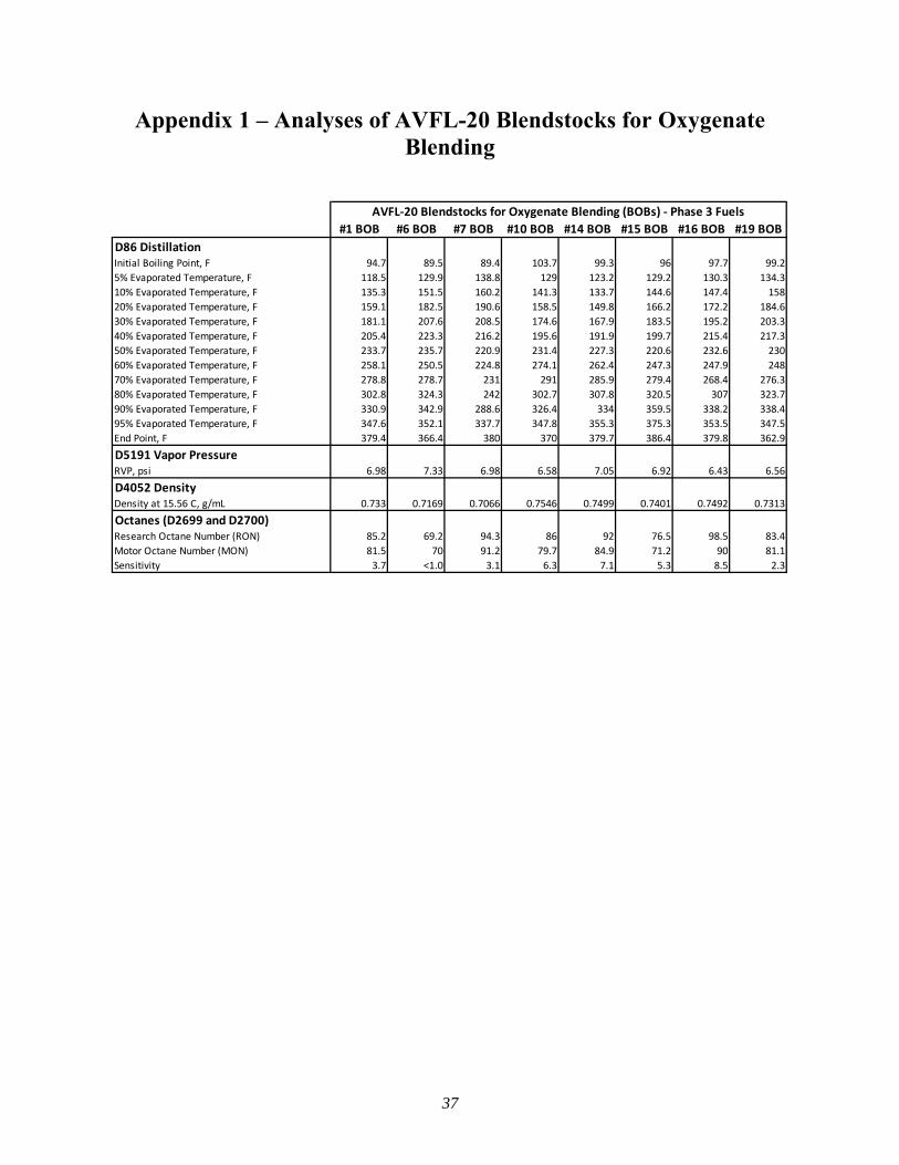
37
Appendix 1 ‒ Analyses of AVFL-20 Blendstocks for Oxygenate
Blending
#1 BOB #6 BOB #7 BOB #10 BOB #14 BOB #15 BOB #16 BOB #19 BOB
D86 DistillationInitial Boiling Point, F 94.7 89.5 89.4 103.7 99.3 96 97.7 99.2
5% Evaporated Temperature, F 118.5 129.9 138.8 129 123.2 129.2 130.3 134.3
10% Evaporated Temperature, F 135.3 151.5 160.2 141.3 133.7 144.6 147.4 158
20% Evaporated Temperature, F 159.1 182.5 190.6 158.5 149.8 166.2 172.2 184.6
30% Evaporated Temperature, F 181.1 207.6 208.5 174.6 167.9 183.5 195.2 203.3
40% Evaporated Temperature, F 205.4 223.3 216.2 195.6 191.9 199.7 215.4 217.3
50% Evaporated Temperature, F 233.7 235.7 220.9 231.4 227.3 220.6 232.6 230
60% Evaporated Temperature, F 258.1 250.5 224.8 274.1 262.4 247.3 247.9 248
70% Evaporated Temperature, F 278.8 278.7 231 291 285.9 279.4 268.4 276.3
80% Evaporated Temperature, F 302.8 324.3 242 302.7 307.8 320.5 307 323.7
90% Evaporated Temperature, F 330.9 342.9 288.6 326.4 334 359.5 338.2 338.4
95% Evaporated Temperature, F 347.6 352.1 337.7 347.8 355.3 375.3 353.5 347.5
End Point, F 379.4 366.4 380 370 379.7 386.4 379.8 362.9
D5191 Vapor PressureRVP, psi 6.98 7.33 6.98 6.58 7.05 6.92 6.43 6.56
D4052 DensityDensity at 15.56 C, g/mL 0.733 0.7169 0.7066 0.7546 0.7499 0.7401 0.7492 0.7313
Octanes (D2699 and D2700)Research Octane Number (RON) 85.2 69.2 94.3 86 92 76.5 98.5 83.4
Motor Octane Number (MON) 81.5 70 91.2 79.7 84.9 71.2 90 81.1
Sensitivity 3.7 <1.0 3.1 6.3 7.1 5.3 8.5 2.3
AVFL-20 Blendstocks for Oxygenate Blending (BOBs) - Phase 3 Fuels

38
Appendix 2 ‒ Analyses of Fuels Working Group Fuels Matrix
Blendstocks for Oxygenate Blending
The finished bioreformate surrogate and wood-derived biogasoline fuels were not blended with
oxygenates; the term BOB (blendstock for oxygenate blending) was retained for the petroleum-based
hydrocarbon portion of these fuels. No analyses of the BOBs for the wood-derived biogasoline fuels were
completed.
#18
BOB
#20
BOB
BRS1
BOB
BRS 2
BOB
BRS 3
BOB
BRS 4
BOB
D86 DistillationInitial Boiling Point, F 93 97.7 90.3 82.5 86.3 84.5
5% Evaporated Temperature, F 127.9 130.4 117.1 109.5 115.4 109.5
10% Evaporated Temperature, F 147.9 149.3 129.7 121.1 133.1 128.4
20% Evaporated Temperature, F 178.9 178.6 151.3 138.5 165.9 156.7
30% Evaporated Temperature, F 203.9 203.1 172.6 155.9 200.2 184.1
40% Evaporated Temperature, F 225 227.7 194.4 174.4 224.8 210.5
50% Evaporated Temperature, F 243.4 252 216.2 193.9 237.6 225.1
60% Evaporated Temperature, F 262.8 273.9 235.6 214.1 248.3 234.2
70% Evaporated Temperature, F 289 296.2 253 232.6 262.5 243.6
80% Evaporated Temperature, F 319.9 317.8 278.7 249.7 289.2 261
90% Evaporated Temperature, F 338.2 336.8 327.1 282.5 326.1 307.4
95% Evaporated Temperature, F 350.8 349.5 354.1 324.3 346.9 337
End Point, F 377.8 375.2 382.2 374 376.3 373.2
D5191 Vapor PressureRVP, psi 6.86 6.41 8.65 9.92 8.55 10.02
D4052 DensityDensity at 15.56 C, g/mL 0.752 0.756 0.737 0.707 0.753 0.724
Octanes (D2699 and D2700)Research Octane Number (RON) 92.3 86.4 96.1 91.3 100.4 98
Motor Octane Number (MON) 86.1 82.2 87 85.6 90.2 89.8
Sensitivity 6.2 4.2 9.1 5.7 10.2 8.1
FWG Fuels Matrix - BOBs

39
Appendix 3 ‒ Analyses of Fuels Working Group Finished Fuels
#18 #20 BRS1 BRS2 BRS3 BRS4 WBG2 WBG4
D86 DistillationInitial Boiling Point, F 102 102 91 90 87 90 83 84
5% Evaporated Temperature, F 128 126 116 118 115 118 102 106
10% Evaporated Temperature, F 140 140 131 134 135 140 118 123
20% Evaporated Temperature, F 152 152 156 161 174 183 146 151
30% Evaporated Temperature, F 159 159 180 187 211 219 177 180
40% Evaporated Temperature, F 163 163 204 213 233 237 205 206
50% Evaporated Temperature, F 166 167 227 236 244 248 225 225
60% Evaporated Temperature, F 236 245 245 254 256 261 240 239
70% Evaporated Temperature, F 268 278 264 272 273 280 254 255
80% Evaporated Temperature, F 304 306 293 299 301 306 277 277
90% Evaporated Temperature, F 335 331 329 327 330 332 310 310
95% Evaporated Temperature, F 347 346 353 348 349 349 338 334
End Point, F 369 365 375 373 374 374 382 381
D5191 Vapor PressureRVP, psi 7.76 7.60 7.86 7.59 7.91 7.49 10.43 9.75
D4052 DensityDensity at 15.56 C, g/mL 0.7596 0.763 0.7511 0.7549 0.7657 0.7672 0.7541 0.7568
Octanes (D2699 and D2700)Research Octane Number (RON) 101.3 97.3 97.3 97.1 101.5 101.6 97.6 97.6
Motor Octane Number (MON) 88.8 87.2 87.4 87.3 90.4 90.4 88.3 88.2
Sensitivity 12.5 10.1 9.9 9.8 11.1 11.2 9.3 9.4
D5291 Elemenal CompositionCarbon Content (wt%) 79.10 79.08 86.87 86.98 87.60 87.28 87.12 87.16
Hydrogen Content (wt%) 13.70 13.60 13.42 13.26 12.82 12.86 12.90 12.84
D4809 Heat of CombustionGross (kJ/kg) 42,645 42,584 46,092 45,859 45,555 45,676 45,811 45,666
Net (kJ/kg) 39,737 39,698 43,244 43,045 42,833 42,945 43,074 42,941
D5599 Oxygenate DeterminationEthanol Content (vol%) 20.08 20.12 0 0 0 0 0 0
Total Oxygen (wt%) 7.28 7.27 0 0 0 0 0 0
FWG Fuels Matrix - Finished Fuels
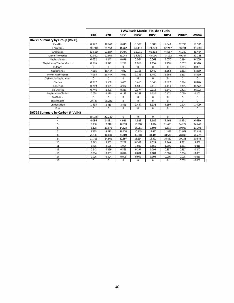
40
#18 #20 BRS1 BRS2 BRS3 BRS4 WBG2 WBG4
D6729 Summary by Group (Vol%)Paraffin 8.172 10.740 8.040 8.300 6.989 6.843 12.798 10.581
I-Paraffins 38.710 31.553 41.767 40.113 39.873 42.217 38.791 39.780
Aromatics 23.560 23.887 34.401 35.910 46.218 44.557 41.200 41.494
Mono-Aromatics 22.522 22.869 33.044 34.780 45.000 43.192 40.307 40.738
Naphthalenes 0.052 0.047 0.078 0.064 0.061 0.070 0.284 0.209
Naphtheno/Olefino-Benzs 0.986 0.971 1.278 1.066 1.157 1.295 0.607 0.546
Indenes 0 0 0 0 0 0 0.003 0.001
Naphthenes 7.065 10.447 7.932 7.755 3.440 2.664 5.363 5.860
Mono-Naphthenes 7.065 10.447 7.932 7.755 3.440 2.664 5.363 5.860
Di/Bicyclo-Naphthenes 0 0 0 0 0 0 0 0
Olefins 0.992 1.580 5.400 5.465 0.348 0.522 0.874 0.876
n-Olefins 0.219 0.189 4.902 4.833 0.110 0.111 0.305 0.272
Iso-Olefins 0.746 1.221 0.313 0.374 0.218 0.240 0.471 0.502Naphtheno-Olefins 0.028 0.170 0.185 0.258 0.020 0.172 0.099 0.102
Di-Olefins 0 0 0 0 0 0 0 0Oxygenates 20.146 20.280 0 0 0 0 0 0
Unidentified 1.355 1.513 2.461 2.457 3.131 3.197 0.974 1.409Plus 0 0 0 0 0 0 0 0
D6729 Summary by Carbon # (Vol%)2 20.146 20.280 0 0 0 0 0 0
4 4.086 3.831 4.918 4.925 5.649 5.463 8.391 6.6805 8.238 7.718 14.839 13.908 13.814 11.405 14.222 14.247
6 8.128 11.976 14.623 14.081 3.693 3.511 10.082 11.291
7 8.225 9.012 11.570 10.215 16.497 11.865 22.071 22.658
8 25.130 18.039 29.609 30.848 33.445 38.520 28.046 28.227
9 11.712 14.961 12.397 15.294 15.391 16.850 10.251 10.548
10 9.943 9.853 7.251 6.362 6.524 7.146 4.291 3.860
11 2.785 2.585 1.954 1.606 1.551 1.696 1.283 0.818
12 0.242 0.226 0.366 0.294 0.298 0.337 0.357 0.247
13 0.004 0.003 0.012 0.004 0.003 0.004 0.014 0.003
14 0.006 0.004 0.001 0.006 0.004 0.005 0.015 0.010
15 0 0 0 0 0 0 0.003 0.002
FWG Fuels Matrix - Finished Fuels

41
Appendix 4 ‒ Values from Engine/Vehicle Study Provided as Inputs
to Life-Cycle Analysis
Volumetric Fuel Economy Values
E10 equivalent volumetric fuel economy values are calculated based on the average properties of CRC
AVFL-20 fuels #1 and #10 (111,986 BTU/gallon).
3 ON/CR 3.7 ON/CR 5.6 ON/CR
14 96.6 112486 10.4 28.4 28.2 28.0
20 97.3 108736 20 27.7 27.5 27.3
6 96 101917 30 25.9 25.8 25.6
15 96.5 103097 30.4 26.3 26.1 25.9
BRS1 97.6 116602 0 29.4 29.2 29.0
BRS2 97.3 116652 0 29.4 29.2 29.0
WBG2 97.7 116607 0 29.5 29.3 29.0
WBG4 97.3 116663 0 29.4 29.2 29.0
7 100.1 108373 10.1 27.8 27.6 27.3
16 101.1 112572 10.2 29.0 28.8 28.4
18 101 108358 20 28.0 27.8 27.5
19 101 101966 29.9 26.5 26.3 26.0
BRS3 101.5 117738 0 30.2 30.0 29.6
BRS4 101.6 118278 0 30.3 30.1 29.8
Fuel ID RON
Heating Value
(BTU/gallon)
Ethanol
Content
(Vol%)
Fleet-Average On-Road Fuel Economy, MPG
3 ON/CR 3.7 ON/CR 5.6 ON/CR
14 96.6 112,486 10.4 28.3 28.1 27.9
20 97.3 108,736 20 28.5 28.4 28.1
6 96 101,917 30 28.5 28.3 28.1
15 96.5 103,097 30.4 28.6 28.4 28.2
BRS1 97.6 116,602 0 28.3 28.1 27.8
BRS2 97.3 116,652 0 28.2 28.1 27.8
WBG2 97.7 116,607 0 28.3 28.1 27.8
WBG4 97.3 116,663 0 28.2 28.1 27.8
7 100.1 108,373 10.1 28.7 28.5 28.2
16 101.1 112,572 10.2 28.8 28.6 28.3
18 101 108,358 20 29.0 28.8 28.4
19 101 101,966 29.9 29.1 28.9 28.6
BRS3 101.5 117,738 0 28.7 28.5 28.2
BRS4 101.6 118,278 0 28.7 28.5 28.2
Fuel ID RON
Heating Value
(BTU/gallon)
Ethanol
Content
(Vol%)
Fleet-Average On-Road Fuel Economy, MPGE10

42
Biogenic Energy Use and Tailpipe CO2 Emissions Values
3 ON/CR 3.7 ON/CR 5.6 ON/CR
14 96.6 11.1 10.4 277 279 281
20 97.3 10.7 20 553 557 562
6 96 7.5 30 880 886 892
15 96.5 11.6 30.4 878 883 890
BRS1 97.6 10.4 0 392 395 398
BRS2 97.3 10.3 0 1178 1186 1196
WBG2 97.7 10.2 0 206 207 209
WBG4 97.3 10.2 0 619 623 628
7 100.1 7.6 10.1 277 279 282
16 101.1 11.8 10.2 268 270 273
18 101 12 20 545 549 555
19 101 12 29.9 869 875 886
BRS3 101.5 11.1 0 382 385 390
BRS4 101.6 11.2 0 1143 1151 1165
Fuel ID RON Sensitivity
Ethanol
Content
Fleet-Average On-Road Energy Use, BTU/mile
3 ON/CR 3.7 ON/CR 5.6 ON/CR
14 96.6 76.621 10.4 21 21 21
20 97.3 77.011 20 41 42 42
6 96 74.657 30 66 66 67
15 96.5 76.503 30.4 66 66 67
BRS1 97.6 77.661 0 34 34 34
BRS2 97.3 78.118 0 101 101 102
WBG2 97.7 78.191 0 21 21 21
WBG4 97.3 78.47 0 63 63 64
7 100.1 73.913 10.1 21 21 21
16 101.1 76.791 10.2 20 20 20
18 101 76.955 20 41 41 42
19 101 75.647 29.9 65 66 67
BRS3 101.5 79.065 0 33 33 33
BRS4 101.6 78.57 0 98 98 100
Fuel ID RON
Total CO2
Intensity (mg
CO2 / BTU)
Ethanol
Content
(Vol%)
Fleet-Average On-Road Biogenic
Tailpipe CO2, g/mile

43
Petroleum-Derived Energy Use and Tailpipe CO2 Emissions Values
3 ON/CR 3.7 ON/CR 5.6 ON/CR
14 96.6 11.1 10.4 3,681 3,704 3,734
20 97.3 10.7 20 3,370 3,393 3,424
6 96 7.5 30 3,050 3,068 3,091
15 96.5 11.6 30.4 3,040 3,060 3,085
BRS1 97.6 10.4 0 3,568 3,592 3,625
BRS2 97.3 10.3 0 2,788 2,806 2,831
WBG2 97.7 10.2 0 3,752 3,777 3,813
WBG4 97.3 10.2 0 3,347 3,369 3,399
7 100.1 7.6 10.1 3,621 3,647 3,689
16 101.1 11.8 10.2 3,617 3,642 3,686
18 101 12 20 3,320 3,343 3,384
19 101 12 29.9 2,975 2,996 3,033
BRS3 101.5 11.1 0 3,520 3,544 3,586
BRS4 101.6 11.2 0 2,758 2,777 2,810
Fuel ID RON Sensitivity
Ethanol
Content
Fleet-Average On-Road Energy Use, BTU/mile
3 ON/CR 3.7 ON/CR 5.6 ON/CR
14 96.6 76.621 10.4 282 284 286
20 97.3 77.011 20 261 262 265
6 96 74.657 30 227 229 230
15 96.5 76.503 30.4 234 235 237
BRS1 97.6 77.661 0 274 276 278
BRS2 97.3 78.118 0 209 210 212
WBG2 97.7 78.191 0 289 291 293
WBG4 97.3 78.47 0 249 250 253
7 100.1 73.913 10.1 267 269 272
16 101.1 76.791 10.2 278 280 284
18 101 76.955 20 256 258 261
19 101 75.647 29.9 225 227 230
BRS3 101.5 79.065 0 276 278 281
BRS4 101.6 78.57 0 209 210 213
Fuel ID RON
Total CO2
Intensity (mg
CO2 / BTU)
Ethanol
Content
(Vol%)
Fleet-Average On-Road Petroleum-Derived
Tailpipe CO2, g/mile

44
Total Energy Use and Tailpipe CO2 Emissions Values
3 ON/CR 3.7 ON/CR 5.6 ON/CR
14 96.6 11.1 10.4 3,958 3,983 4,015
20 97.3 10.7 20 3,924 3,950 3,986
6 96 7.5 30 3,930 3,953 3,983
15 96.5 11.6 30.4 3,918 3,943 3,975
BRS1 97.6 10.4 0 3,960 3,986 4,023
BRS2 97.3 10.3 0 3,966 3,992 4,027
WBG2 97.7 10.2 0 3,958 3,985 4,022
WBG4 97.3 10.2 0 3,966 3,992 4,027
7 100.1 7.6 10.1 3,898 3,925 3,971
16 101.1 11.8 10.2 3,885 3,912 3,959
18 101 12 20 3,865 3,892 3,939
19 101 12 29.9 3,844 3,871 3,919
BRS3 101.5 11.1 0 3,902 3,929 3,976
BRS4 101.6 11.2 0 3,901 3,927 3,975
Fuel ID RON Sensitivity
Ethanol
Content
(Vol%)
Fleet-Average On-Road Total
Energy Use, BTU/mile
3 ON/CR 3.7 ON/CR 5.6 ON/CR
14 96.6 76.621 10.4 303 305 308
20 97.3 77.011 20 302 304 307
6 96 74.657 30 293 295 297
15 96.5 76.503 30.4 300 302 304
BRS1 97.6 77.661 0 308 310 312
BRS2 97.3 78.118 0 310 312 315
WBG2 97.7 78.191 0 310 312 314
WBG4 97.3 78.47 0 311 313 316
7 100.1 73.913 10.1 288 290 293
16 101.1 76.791 10.2 298 300 304
18 101 76.955 20 297 300 303
19 101 75.647 29.9 291 293 296
BRS3 101.5 79.065 0 309 311 314
BRS4 101.6 78.57 0 307 309 312
Fuel ID RON
Total CO2
Intensity (mg
CO2 / BTU)
Ethanol
Content
(Vol%)
Fleet-Average On-Road Total
Tailpipe CO2, g/mile