U.S. DEPARTMENT OF THE INTERIOR

U.S. GEOLOGICAL SURVEY

The generation of raster-format geologic maps using digital image- processing on the Macintosh computer: A tutorial guide

by Christopher D. Condit1 *2 and Alex V. Acosta1

Open File Report-93-526

Report includes 5 text files, 4 program files, 59 image files, 15 ASCII data files, and 18 CLUT files in self-extracting archives on two diskettes

This report is preliminary and has not been reviewed for conformity with U.S. Geological Survey editorial standards (or with the North American Stratigraphic Code). The following commercial programs, companies, and hardware are mentioned in this report: Aladdin, Canvas, DeskWriter C, Hewlett Packard, HyperCard, Lightsource, Microsoft Word, Microsoft Excel, Ofoto, Optronics, PaintJet XL300, Stuffit Lite, SuperCard. Any use of trade, product or firm names is for descriptive purposes only and does not imply endorsement by the U.S. Government.

Although CLUTMake and GrayMap programs have been used by the U.S. Geological Survey, no warranty, expressed or implied, is made by the USGS as to the accuracy and functioning of the programs and related program material, nor shall the fact of distribution constitute any such warranty, and no responsibility is assumed by the USGS in connection therewith.

1 Flagstaff Field Center, U.S. Geological Survey, 2555 N. Gemini Dr., Flagstaff,AZ 86001

^Department of Geology and Geography, University of Massachusetts, Amherst,MA 01003

AbstractThis report is a tutorial guide to the use of digital image processing on the

Macintosh computer as a tool for map generation. The procedures described will enable the reader to produce digital maps in raster or bit-mapped format that are stored within the computer. Included are various programs and image and data files to be used with the report.

Each section of this report takes a sequentially more detailed look into the process of map-making on the Macintosh computer. We focus first on the mechanics of program utilization, then on details of using image-processing techniques for generation of maps. We outline conventions and terminology common to image processing, and we summarize the layout of the NIH Image program, the main tool used for map generation in this tutorial, describing its main functions and the primary uses of its display windows and tools. We then concentrate on the uses of NIH Image for map production, first giving an overview of what is involved in making a digital map. We next describe these steps in more detail, and with the use of supplemental images, give step-by-step instructions on how NIH Image can be used to create a desired product. The last part of this section gives information on how we link ancillary data with a map image and illustrates how this combination can be used to make thematic maps. We then take the reader through the process of converting the image files of a single gray-scale map into three different color thematic maps. We show how one can reduce map scale, transform maps with more than 256 units to maps with fewer units, and mosaic map segments together. Finally, we describe supplemental procedures applicable to specific parts of map-making, including the use of NIH Image to generate ASCII files of measurements (for example, areas of map units), the use of a data-compression program (Stuffif), and the encoding of a BINHEX file, a process needed before files can be transmitted by electronic mails.

We include three Appendices: the first gives some background on the example data base; the second lists the computer files included with this report; and the third summarizes the main steps of map generation.

i

Table of Contents Page1. Introduction 1

1.1 Recent work 21.2 Scope and use of report 31.3 System requirements 5

2. General conventions 52.1 File formats 52.2 Image-file headers 62.3 DN values 72.4 Files and conventions used in this report 8

3. The NIH Image program: A brief introduction 83.1 Windows, Menus and Tools 83.2 Memory management 11

4. Basic Procedures 124.1 An overview of ExAIl.Pict 124.2 Working with ExAIl.Pict 13

4.2.1 Preparing the base map 134.2.2 Gray-level mapping (contrast stretching) 144.2.3 Generation of unit contacts 164.2.4 Line-thinning of contacts 184.2.5 Editing contacts and filling polygons 194.2.6 Bit-mapped layers and adding labels/symbols 21

4.2.6.1 Compositing (combining or overlaying) files 214.2.6.2 Adding text to files 224.2.6.3 Separating single DN value

layers from images 234.2.6.4 The use of Density Slicing 23

4.2.7 Creating palettes and LUTs 244.2.7.1 Creating ASCII input files for CLUTMake 244.2.7.2 Color codes for ASCII files from the

USGS Process Ink Color Chart 254.2.7.3 Using CLUTMake 264.2.7.4 Importing CLUTs into a file 27

4.2.8 Making thematic derivatives: the data base link 275. Building Thematic Maps: An Example 286. Dealing with Large Maps and

Large Numbers of Units 336.1 Introduction 336.2 Outline of procedures 336.3 Scale reduction 346.4 DN value transformations 36

ii

6.5 Mosaicking 406.6 Creating Multiple Thematic Maps 41

7. Supplemental Procedures 437.1 A note about fonts with Microsoft Word 437.2 Additional techniques and short cuts for NIH Image 43

7.2.1 How to set a map scale 437.2.1.1 Method 1 447.2.1.2 Method 2 44

7.2.2 How to obtain areal measurements and savethem in ASCII (tab delimited) files 44

7.2.3 How to obtain and save histogrammeasurements in ASCII file 45

7.2.4 How to make thick contacts/lines (3 pixels wide) 457.2.5 How to create one-pixel-wide contacts around filled polygons 45

7.3 File compression/decompression, BINHEX encode/decodeand file segmentation procedures with Stuffit 467.3.1 How to "Unstuff* files compressed on disk 467.3.2 How to "Stuff or compress files on disk 477.3.3 How to encode/decode a BINHEX file using Stuffit 477.3.4 File segmentation/joining using Stuffit 48

7.4 Additional techniques 497.4.1 How to calculate the number of lines and samples

to be created from a SCITEX scan 497.4.2 How to calculate the number of blocks of disk

space used by an image operating using the VMS PICS system 49

8. Acknowledgments 499. References Cited 49 Appendix IA. The thematic maps of the

Springerville Volcanic Field. 51Appendix IB, An explanation of ExAll.Pict 53Appendix II: Computer files included with this manuscript 54

A. Text 54B. Programs 55C. NIH Images (in Pict format, listed by order of use) 55D. DNMAP files (ASCII format) 56E. GLUTS (palettes) 56F. USGS Color Code (Image) Files 57

Appendix III: List of steps to map generation 58Figure 1 9

iii

1. INTRODUCTIONThe timely and efficient publication of geologic maps is costly and

time consuming. To help solve these and associated problems, the U.S. Geological Survey (USGS), as part of its map modernization effort, has funded a program to generate geologic maps by using digital image processing. A part of this program emphasizes on use of the desk top computer. This report focuses on the use of digital image processing on the Macintosh computer as a tool for map generation.

The need for map modernization is clear. The manual preparation methods used up to now are expensive: geologists and technical support personnel are required to spend inordinate amounts of time in such preparation. Production of most maps involves at least two generations of drafting; color maps often require several versions of peel-coat preparation. The final product is usually difficult to update, and it is cumbersome to correlate with ancillary data.

One solution to these problems is the use of digital image processing to produce maps, a technique that has been used with great success in planetary science (for example, Greeley and Batson, 1990). A major problem with this method of map generation has been the necessary use of main frame computers for image processing. Aside from the costs, this dependence on such computers restricts access for the geologist who is generating maps. Further, most image processing systems on mam frame computers are complex and difficult to use, therefore less palatable to the geologist. Recently developed image processing software for desk top computers such as the Macintosh provides intuitive, user-friendly, moderately priced, and widely available platforms for such work.

The use of digital image processing to compile maps offers the possibility of eliminating much of the time-consuming efforts of the geologists and technical support personnel and also much of the cost associated with the production of color maps. In addition, digital image processing solves several other problems. A map, once generated as a digital image, can be used both in digital form on the computer, and as a means for production of final color separates for hard-copy (paper) maps. By transferring line work directly from paper field maps to computer files (for example, to a scanned topographic image of the same area), by using a drawing tool in an image processing program, the rendering of these lines

1

is reduced to a single effort. Lines need never be drafted again, and they are accurately registered to the topographic base as input by the mapper. Once mapped exposures are filled with a distinctive identifying color or gray-scale brightness value (for example, by using a "paint" program), image processing techniques can be used to translate these fill values to final map colors selected by the geologist. The colored digital image files can then be used to generate the final color separates for hard-copy map production. In addition, the original filled image can be used as a base for production of any number of color thematic maps, and it can be updated quickly and efficiently. Other advantages accrue if the fill values of units on the digital image are associated with an ASCII file (or spread-sheet) of ancillary laboratory data (for example, geochemical or geophysical data). The use of associative programs such as SuperCard and HyperCard now make it possible to directly link ancillary data to image space. This link offers scientists who use large, geographically correlated data sets an efficient means to publish their data. Digital images and associated ASCII files can be rapidly disseminated by E-mail, or on diskettes; large files can be sent on CDs, where they can also be archived. Digital images offer additional advantages because the data can be used by Geographic Information System (GIS) programs, and they can also be easily reduced in scale, thus making large-scale summary maps much easier to produce from more detailed small-scale maps. 1.1 Recent work

To date four experimental l:100,000-scale geologic thematic maps of the Springerville volcanic field in east-central Arizona (449 units, «3000 km^) have been produced (Acosta and others, 1989; Condit and others, 1989; Condit and others, in press). These maps were initially generated by using programs of the VAX-based Planetary Imaging Cartography System (PICS) in Flagstaff. The maps represent an outgrowth of techniques developed by Acosta over the last several years on other experimental maps produced for geologists at the Flagstaff Field Center. For hard-copy, the Springerville maps were based on the software developed by Acosta and Barrett (1990) to produce directly the color separates [on a small-format (10"xlO") Optronics film writer] needed for lithographic printing, thus avoiding the traditional and time-consuming peel-coat process. These four thematic maps and others being produced by

2

Acosta in collaboration with other workers are being evaluated for conformity with USGS standards for hard-copy map quality. The goal of this research is to use the system presented in this report as a means of producing raster-format maps for the USGS. The use of raster-format in combination with vector-format is essential: most of the topographic map bases cannot be easily converted to vector form, hence most digital maps must be produced in some sort of combination raster (bit-mapped) and vector form. Because a primary goal of this project is to bring map- making capabilities into the desk top environment, our recent work has resulted in the transfer of almost all of the capabilities inherent only in main frame or micro computer environments to the Macintosh computer, and all maps produced to date have included varied amounts of processing on the Macintosh . Much of the effort has centered around the use of the public domain software package "Image" developed by Wayne Rasband at the National Institute of Health (herein referred to as NIH Image to distinguish it from NCSA Image). The most recent version of NIH Image (including the source code, and manual) is available via anonymous FTP from zippy.nimh.nih.gov [128.231.98.32], in directory /pub/image. This tutorial describes techniques using version 1.49 of NIH Image . 1.2 Scope and use of report

The rest of this report describes, in tutorial style, procedures to produce digital maps on the Macintosh. We assume that the user has at least a general level of familiarity with the Macintosh computer. Included with the report are various programs and image and data files to be used hi conjunction with it. (See Appendix II for a list of these files.) These procedures should enable the reader to produce digital maps stored within the computer. Appendix III is a check list of procedures, the experienceduser can use it to bypass any detailed steps hi the tutorial if she is already familiar with them. Additional files (double-underlined) are included thatthe user would create if stepping through the tutorial; these files can be used to compare output at any step, and that can be used hi lieu of files created in the tutorial to facilitate picking up the tutorial at any given step. Future reports will describe (1) map-quality, hard-copy production when the steps for that output are finalized, and (2) the steps involved in combining raster- and vector-format files, most of which involve the use of Computer Assisted Drafting (CAD) programs. In the interim, laser and

3

ink-jet printers (both color and black and white, for example, the Hewlett Packard Deskwriter C and PaintJet XL300) can be used for hard-copy output of the images produced by methods given herein; this hard-copy would include transparencies suitable for overhead projectors.

The rest of this report is divided into six major sections. With the exception of part 2 (GENERAL CONVENTIONS), each section takes a sequentially more detailed look into the process of map-making on the Macintosh computer. In GENERAL CONVENTIONS we outline conventions and terminology common to image processing, especially as applied to the Macintosh. In part 3 (THE NIH IMAGE PROGRAM), we briefly outline the layout of the program, describing its main functions and the primary uses of display windows and tools. Additional, more general information on options and uses of these windows and functions can be can be found in the manual entitled "About Image" by Wayne Rasband and an associated manual entitled "Inside Image" by Mark Vivino, both of which are included in the compressed NIH Image archive on the file server zippy.nimh.nih.gov. Users are encouraged to print out and examine "About Image" and "Inside Image" for a more through background in their use; the program has capabilities far beyond those described in this report. Building on this brief introduction, we then concentrate in part 4 (BASIC PROCEDURES) on the uses of NIH Image for map production. In this section we take a first look at what is involved in making a digital map. First, we briefly introduce the steps followed in making a map by referring to image "ExAll.Pict" Next we describe these steps in more detail, and with the use of supplemental images, we give step-by-step instructions on how NIH Image can be used to create the desired output. The last part of this section gives information on how we link ancillary data with a map image and how this combination can be used to make thematic maps. In section 5 (BUILDING THEMATIC MAPS: AN EXAMPLE), we take the reader through the process of converting the image files of a single gray-scale map into three different color thematic maps by applying different gray-scale-to-color Look Up Tables (LUTs); this section contains a more complete explanation of the application of LUTs to files than that found when working with ExAll.Pict. In part 6 (DEALING WITH LARGE MAPS AND LARGE NUMBERS OF UNITS), we show how one can reduce map scale, transform maps with more than

4

256 units to maps with fewer units, and mosaic map segments together. Finally, in part 7 (SUPPLEMENTAL PROCEDURES), we describe additional procedures applicable to specific parts of map-making including the use of NIH Image to generate ASCII files of measurements (for example, areas of map units), the use of a data-compression program (Stuffit), and the use of Stuffit to encode a BINHEX4 file, a process needed to transmitted the file by e-mail.

All files included with this report are stored in a compressed format as self-extracting-archives (.sea). Before reading past part 3, you should "unStuff these files, following the steps outlined in section 7.3.1 (How to "Unstuff files compressed on disk). 1.3. System requirements

To run NIH Image one needs at least 8 megabytes (MB) of random access memory (RAM); the single most important item in increasing map- making efficiency is RAM; we nominally operate with 32 MB. NIH Image will not run without an 8-bit (256) color card and monitor; 13-inch monitors are at the lower practical limit in size and 16- and 19-inch monitors provide more optimal working conditions. Hard disks are essential, given the large size image (and thus file sizes) of map-making, and removable hard drives (of the 44 or 88 MB sizes) provide a way to back up images and to prevent cluttering an internal hard drive. 2. GENERAL CONVENTIONS 2.1 File formats

File formats of digital images come in two basic forms: raster- and vector-format. An image in a raster-format file is stored as a stream of bytes in which each byte corresponds to a pixel. Each image line corresponds to a part of this byte stream, with lines arranged consecutively in row order (for example, line one is found first in the byte stream, followed by line two, etc.). In Tagged Image File Format (TIFF), files are in raster-format, and although there are several different types of TIFF files, most can be copied from computer to computer and read by most image processing programs. Within the Macintosh, there is another type of file format, called the PICT format. Loosely speaking, PICT files can include (see next paragraph) raster-file format data that have been "run- length-encoded," a scheme whereby any adjacent samples within a line of data that have the same digital number (DN) value can be compressed and

5

stored with only their line number, starting sample, ending sample and DN value. Because map images have large regions of the same DN value, and these files are often much more compact, we recommend saving in PICT format. Such PICT files can be loaded into NIH Image and then saved back to disk in the TIFF format for transfer to other computers with no loss of information. For further information on file compression (and encoding into BINHEX4 format for e-mail transmittal), see part 7 (SUPPLEMENTAL PROCEDURES).

Vector files, the other major type of format, contain their image information as mathematical formulas describing the lines and shapes in an image. Because many images have regions of similar DN values, their storage as vector files is often more compact, because only areas with data are described. Decoding vector files into interpretable images requires information as to the vector-file format (that is, what formulas are used); therefore, they are less transportable between programs and machines. The main advantage of vector files, aside from compact size, is that they are scale independent and can be enlarged or compressed without loss of image resolution. PICT files can include both raster and vector information; generally, if both are included in a given PICT file, the raster data is a run-length encoded "object." 2.2 Image-Hie headers

Most image files contain information, specific to an image- processing program and/or computer, this information precedes the image and is stored as a "header line" or "header." It contains information about the image, for example, its size [number of pixel lines (height of an image), number of pixel samples (width of an image)], and bit type (for example, 8-bit). Some headers contain only an image label with sparse information about the image; others include a label followed by much more detailed information about the image. If in raster-format, files with headers can be imported into NIH Image. The key to importing files into NIH Image lies in knowing the size of the header (that is, the number of bytes), the number of lines and samples in the image, and the length of words (either 8- or 16-bit). For example VAX-based PICS (Planetary Imaging Cartography System) files, which are in raster-format, have headers of 22016 bytes and include a PICS label and, in addition, a detailed history of the processing applied to the image.

6

2.3 DN valuesAll processing using NIH Image is done in raster (bit-mapped)

format. The image is most simply thought of as a "checker-board" of squares, each called a "pixel" or picture element. (For more detailed information see Condit and Chavez, 1979, or any text on image- processing.) Because we use 8-bit data, each pixel is assigned one of 256 shades of gray (corresponding to a DN value); the convention used here, following that of the Macintosh palette, sets a pixel with a DN value of 0 equal to white, a pixel with a DN value of 255 equal to black. In either case, a medium-gray pixel would have a DN value of 127. By using the Options-Preferences Menus and checking the "Invert Displayed Pixel Values" box, one can assign pixels with DN values of 0 to black tones; and pixels with DN values of 255 to white, with intermediate pixel values distributed to gray shades accordingly. To retain any changes in Preferences, all changes in must be recorded (use the File-Record Preferences Menus) and the program restarted. Note that the use of the "Edit-Invert" Menu command completely inverts the DN values so that all pixels with a value of 1 are reassigned to 254, pixels with DN values of 2 are reassigned to 253, etc.

We use these different DN values to separate data within images into major types, which is useful for generating maps. For the first major type of data we assign distinct DN values to different types of black-plate overlays. (For example, all geologic contacts might be drawn in with a DN=255, all labels or map symbols typed in with a DN=253, and all topography assigned DN=127.) By compiling data using different DN values, as described below, one can isolate each data set and save each as a separate file for use as a series of black-plate overlays. Subsequently, various thematic maps can be quickly generated by combining different layers (or overlays) together (either in the computer or photographically during final map production.)

The second major type of data to which we assign distinct DN values is that used to fill polygons corresponding to the outcrop areas of different geologic units. For this use, each polygon corresponding to a different unit is filled ("painted") with a unique shade of gray (DN value). This "filled polygon" file can then be manipulated to generate different colors for the polygons, depending on the attribute examined in the thematic map

7

(for instance, a unit with a DN value of 27 could be colored blue for a lithologic map, but red for a magnetic map). This type of manipulation is done by creating "Color-Look-Up Tables" that assign a specific DN value, or range of DN values to a given color, as covered below in the section 4.2.7, "Creating palettes and LUTS". 2.4 The files and conventions used in this report

All image files included with this report will be underlined for ease of recognition (for example ExAll.Pict). As noted above, double = underlined file names (for example, SVFls 16CRegistr) indicate examplesof the final files created by the user at the end of a series of steps along the way; these files can be used for comparative purposes and by the user who wishes to jump into a process without having to create products in previous procedures. All program files in this report are in italics (for example, NIH Image, CLUTMake, GRAYMap). Also, many of the tools and functions referred to in this report can be invoked by locating the cursor over its associated icon (picture or symbol) and clicking the button on the mouse or track ball. When first introduced, any icon discussed will be included within the text (for example the pencil tool, used for drawing, looks like this: ff). Many of the images used in this report were derived from a map used in a pilot study on map modernization sponsored by the National Geologic Mapping Program. The area chosen for this map is the Springerville volcanic field, located in east-central Arizona. For more information about the map used see Appendix I, and MI-1993 (Condit, 1991) and Condit and others, 1989, and in press. 3. "THE NIH Image PROGRAM: A BRIEF INTRODUCTION 3.1 Windows, Menus and Tools

If you have not done so, decompress and save all files to your hard disk following the steps outlined in section 7.3.2.

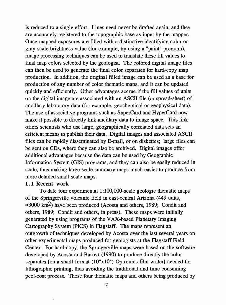
When started, NIH Image appears with five basic windows beneath the Main Menu bar at the top of the screen, each with a different function or information (Figure 1). To start the program and load an image, find the folder containing the file Active Image Window, and click on it twice. (You can also start the program by double-clicking on the icon NIH Image, which loads the program with no active image). From left to right at the top, the windows include (1) the LUT (Look Up Table) Window, (2) the Tools Window, and (3) the active Image Window (with the text "Active

8

image window" in it). On the lower left, below the LUT and Tools windows, are (4) the Map Window and (5) the Values Window (they are

File Edit Options Enhance Rnalyze Special Stacks Windows

Map

-| |

Active image window

UaluesX: 170V:60UaIue:60

Pixels: 60000 Mean: 0.16 Std Dev: 3.06 Min: 0.00 Max: 60.00 Length: 1000.00

Untitled

Inactive image window

a

Paste Control

Transfer Mode [ flddCopy [Subtract

Scale Math H {"""'P'HJ Liue PasteD I Diu'de j

Figure 1 . The five basic types of windows used by NIH Image, and the Paste Control window. (See text for explanation.)

overlapping on a 13" monitor.) The Main Menu bar at the top contains additional functions (for example, in the File Menu, Save), and for some

9

functions, Submenus. In many cases one can interchangeably activate a function from a Window (by clicking on a Tool icon, thus selecting it), from a Menu selection, or by using a keyboard short cut. To work in a window, or to select it (that is to bring it to the front if it is overlapped by another window), point and click in the desired window. If you are operating under System 7, you can activate Balloon Help as another means of familiarizing yourself with this program (on versions 1.49 and higher); it is especially helpful for attaching names to the tool icons, and, as long as the window beneath the cursor is active, it yields a summary of the use of the tool or window.

The LUT Window contains a vertically arranged gray or color bar showing the full range of gray tones or colors possible hi the active Image Window. The precise DN values relating the gray or color can be found by pointing (the pointer becomes an eye dropper icon * ) in the LUT Window to a gray tone or color; the corresponding DN value is then listed in the Values Window below.

The Tools Window contains icons that, when selected, activate a function that can then be implemented, within either the Image Window or the LUT Window. For example, clicking on the pencil V , and then selecting (clicking on) a DN value in the LUT window gives the capability to then click and drag the pencil across the image in the active Image Window and to draw a line beneath the pencil point. This line will have the DN value selected within the LUT Window.

The active Image Window contains the image being worked on or viewed. Additional images can be loaded into Image Windows, their number depending on (1) total RAM memory of the computer and that assigned to the application, in this case NIH Image, (2) the image sizes, (3) the number of images loaded, and (4) the size of the Undo and Clipboard buffers (areas of RAM memory used for storing images being edited or transformed; see section 3.2 (below). Note in Figure 1 that the active window has horizontal lines at the top; by clicking on the top bar, and dragging and releasing where you wish to relocate it, one can move the active window around the screen (try it).

The Map Window contains a square graph showing the brightness and contrast of the active image data. Beneath this graph are two scales,

10

one showing the brightness level BI mz3 ? the other the contrast level c» =3. Clicking and dragging either on the line within the graph or on the black squares within the two scales allows these levels to be dynamically changed within the active image (try it).

The Values Window contains information that is dependent on which window is active. When the LUT Window is active, the Values Window contains DN values beneath the tip of the eye dropper * (which is what the cursor transforms to when hi the LUT Window). However, when a tool is being used hi the active Image Window, the Values Window displays the sample and line coordinates and the associated DN value beneath the tool (for example, in Figure 1, the cursor can be found at sample 170 (top line - x:170), line 60 (second line - y:60); the DN value (third line Value: 60). When an area is edited or selected, its size (width and height) is shown. 3.2 Memory management

NIH Image uses Undo and Clipboard buffers, each of which are ideally equal to or larger than the size of the image in the active Image Window. These buffers limit the maximum size that an image can load to about one-third the size of RAM assigned to the program, if you wish to retain complete editing capabilities (for example, an overlay operation, wherein one entire image is superposed into another). For this reason, for general use, we recommend running NIH Image under System 7 with extensions off, unless you are fortunate enough to have more than 8 megabytes of RAM. To start with extensions off, click on the Special Menu, and drag down to Restart, something one should do anyway if other users have been working with the computer, or other applications have been running. Then hold the Shift key down until the pop-up window "Welcome to Macintosh - Extensions off appears. To determine the amount of free RAM your computer has, with no program loaded, click on the Apple w (left side, top menu bar), and drag and release on "About this Macintosh." A window appears showing the amount of free RAM and the amount of RAM the system is using. Generally, when running under system 7, the system works fine with about 1500 K bytes (for a more exact figure, see your window).

Aside from operating the Macintosh with extensions off, there are two ways to set memory in order to maximize RAM available when using

1 1

NIH Image. First, single-click on the program icon, and use the keys Command-L (Note that the "Command" keys are the ones with the ^ ^ just left and right of the space bar). A window with information about the program appears. Set the application memory size to about 500 K less than your total available RAM. (If you have an eight MB machine, try 6700 K for use with this tutorial.) Next, start NIH Image, and under the Options Menu, select the Preferences Submenu. On the pop-up window set your Undo and Clipboard buffers to about 300 K less than one-third of the size you set for your application memory . Do this by clicking in the box showing the size and editing the value found in that box (set the buffers to 1634 K for use with this tutorial). Follow the prompts to the File Menu- Record Preferences, Quit and the restart the program at this point. This should maximize the image size available when using NIH Image. 4. BASIC PROCEDURES 4.1 An overview of ExAlLPict

If you have not already done so, start NIH Image, select "Open" from the File Menu, and double click on the file ExAlLPict. This file contains nine frames encapsulating steps used in map generation. First, we'll scan through these nine frames to gain an overview of the steps to building a raster-format map, and then, with the use of supplemental images, we'll walk through each step in detail. When we compare the tutorial procedures described in this section with those displayed hi the image ExAll.Pict several discrepancies will become apparent. These result because we simulate, in a single image, the conversion of a gray­ scale image into three different color thematic maps; the differences caused by this simulation will be briefly noted in the text. A more complete explanation is in the Appendix IB, "Explanation of ExAlLPict". In section 4.2.8, Making Thematic Derivatives, many of the steps encapsulated here will be further explained while you are working on other supplemental files.

Frame 1 (upper left) of image ExAlLPict shows the first step of map generation, that of drawing contacts on a topographic image. In the next frame (center, top) we have removed the topographic base from the topography and are in the process of thinning the line work to a single pixel width. In the third frame we build on this by filling the closed contacts with the different gray values assigned to each unit. In Frame 4,

12

we have added the topography back into the filled line work and are adding labels to the units. The center frame shows the result of separating the labels we just added from the rest of the image. At this point, we can save these labels as a separate image, and if we wish, create another label overlay. This flexibility lets us change unit names, etc. to generate different thematic maps. Frame 6 illustrates the process of transforming an image from gray-scale to color. Chosen DN values are assigned to colors by creating a palette used to modify the color-look-up-table (GLUT). This palette is added to the image, modifying the original gray­ scale look-up-table. The bottom three frames illustrate how, by simply changing the GLUT assigned to a single image (by importing different palettes), three different thematic maps can be created. Three insets showing the different thematic classifications have also been created for these bottom frames (Figure 2). A more inclusive example of a lithologic map can be examined in file SVFCSWls2Lith. Close the file SVFCSWls2Lith when you have finished examining it by clicking the close button in the upper left hand corner of its image window. 4.2 Working with ExAll.Pict

Now let's examine the image ExAll.Pict in more detail. We will do this by keeping ExAll.Pict in one window and working with additional images in another Image Window; we will load and remove each additional window when we are done with it. At this stage, experimentation is encouraged; if you should make errors when trying an operation, you can simply close the image (thus removing it from RAM) by clicking on the upper left-hand box in the active Image Window (or by selecting "Close" from the File Menu, or by using the keyboard short cut "Command-W"). Then reload the image from your disk. As long as you don't save any changes when closing the window, you can try as many options as you wish without compromising the supplied data set.

4.2.1 Preparing the base mapImage files of contacts (lines separating geologic units) can be

generated in one of three ways: (a) transferring contacts from a paper copy of a field map to an image file in the computer using the Pencil Tool of NIH Image, (b) by drawing contacts on remotely sensed images that have been geometrically transformed to final map projection, or (c) by

13

scanning line work of a stable-base cronoflex (see section 4.2.4, "Line- thinning of contacts").

To generate a topographic base file for (a) above, we recommend either scanning using a flat-bed scanner and saving directly into PICT file format, or obtaining the image scan from a large-format film writer/scanner such as SCITEX. The topography in image ExAll.Pict was taken from a l:100,000-scale topographic map that had been photo-reduced to 85% and scanned on an Apple Flatbed Scanner at 300 DPI (line-art option). The file was saved in the PICT format. A comparison of this scanned data with that from a SCITEX scan shows a difference between the two files of one pixel in 1000. If you are using a flatbed scanner, software that has an "auto-straighten" option (such as Ofoto by Lightsource) is almost essential if you are planning to mosaic several scans together.

4.2.2 Gray-level mapping (contrast stretching)When using procedure (a), the next step, using NIH Image, is to

convert all topographic data to a single DN value that is different from the value used to draw contacts. For convenience, it should be easy to see but should not confuse contact placement; we have found a gray value of 127 works fine.+

To obtain a histogram of all DN values found in the active image window, select Show Histogram from the Analyze Menu (or use the shortcut Command-H on the keyboard) for the image ExAll.Pict. Running the cursor left and right within the Histogram Window causes the DN value and number of pixels at each DN value to be displayed in the Values Window. In part 7 (SUPPLEMENTAL PROCEDURES), we explain how these histogram values can be saved to an ASCII file for more quantitative analysis of the image data. Note that if a smaller area of the image is

r i

selected (by using the Rectangle Selection Tool from the Tools Window l-J ),the histogram obtained gives values only for pixels within the selected

+ Note that in image ExAll.Pict the contour lines in Frames 1 and 4 have been mapped to DN 252 instead of 127. (Place your cursor over these lines and observe the values in the Results Window.) For clarity, the DN value for contour lines in these two frames has been further assigned a blue color. In Frames 7 to 9 the contours have been remapped to DN 127, and there assigned a gray tone (YMCK=5550; see section 4.2.7 for a discussion of gray-scale-to-color mapping and YMCK nomenclature).

14

area. After noting the range of DN values in the Histogram Window, click the close box in the upper left corner.

When working within NIH Image, you can follow two procedures to convert (or change) DN values (called gray-level mapping or stretching). An additional program used in conjunction with NIH Image , called GRAYMap, described in section 6.4.6 "DN value transformations," gives the user another, more flexible, "Table Stretch" option. Within NIH Image the first option involves converting or changing all pixels with the same single DN value to another DN value; the other involves changing all pixels within a range of DN values to a single DN value. We'll demonstrate the first procedure by working with the image file ExTopo253: use Command-O and double click on this file now. Obtain a histogram of this image, check its values and then close the histogram box. To convert a single DN value (hi this instance to change DN 253 to DN 127), we must first set the foreground DN value to the DN value we wish to change (that is, 253). Go to the Tools Window, click on the Paint Brush

Si , then go to the LUT Window to the left; looking at the Values Window below it, and move the dropper in the LUT Window until GRAY VALUE=253. Then click (this sets the foreground color to DN=253). Next set the background color to DN=127 by clicking the Eraser £r on the Tools Window, and click DN=127 on the LUT. Then select Change Values from the Enhance Menu; by clicking OK, the result will send DN 253 to DN 127. Now, to remove the image ExTopo253 from RAM, click the close box (upper left box in its Image Window). Note that use of the Macro Commands (or Macros) Fl and F2 ("Set Foreground Color" and "Set Background Color" in the Special Menu) allow the user to set the foreground and background to values by typing them directly into a pop­ up window rather than by selecting them through clicking in the LUT Window. An additional Macro (F8, "Change 1 DN value) will also speed up this process. For the set of Macros included with this tutorial to work, the file "Image Macros" must reside in the same folder as the NIH Image program.

Now let's look at the option that involves changing all pixels within a range of DN values to a single DN value. If starting with a spacecraft image (b), (for example, load file 253s47.PictSm). you need to gray-map

1 5

("stretch") to 251 any DN values between 252 and 254, and gray-map to DN 0 to the DN 1 value, in order to reserve those values for line work, symbols, etc. Use Command-H to obtain a histogram; check DN values between 252 and 254 and then close the histogram window. To change all pixels with values between 254 and 252 to a DN value of 251, select "Density Slice" from the "Options Menu" (or double-click on the wand \ in the Tools Window; see section 4.2.6.4 for a more detailed description of Density Slicing). Note that a red horizontal line appears with a vertical double-headed arrow T" (the Palette or LUT Tool) when the cursor is moved to the LUT Window. Looking at the Values Window below the LUT, drag the LUT Tool down to 254 and release the mouse button. Then click on the top of the red "density slice" in the LUT, and drag the red area to a DN value of 252. Then, in the Tools Window, click on the Paint Brush, and then click on DN=251 in the LUT (this sets the foreground color to DN=251, the value to which you wish to send DN 254-252). Next, select "Apply LUT" from the Enhance Menu, and on the pop-up menu, select the top and bottom buttons, and click OK. The result will send all values in the red density slice to DN=251; you can verify this with another histogram if you wish. If there are any DN=0 values, use the procedure described above to change a single DN value from DN=0 to DN=1 (click on the Paint Brush, then click on DN=0 hi the LUT, next click on the Eraser, then click on DN=1 hi the LUT, then select Change Values in the Enhance Menu). NIH Image, following Macintosh protocol, reserves DN values of 255 for black and 0 for white, therefore, to change those values you use not the Threshold Tool, but rather the "Change Values" option. Keep the image 253s47.PictSm in an Image Window for later use. Note that the Macros F8 and F9 ("Change 1 DN value," and "Change Slice of DN," respectively, permit the operations noted above if the user types hi values to pop-up windows.

4.2.3 Generation of unit contactsNow let's copy Frame 1 of the image ExAll.Pict to the clipboard and

draw contacts directly on this copy in the clipboard. (We will look at this procedure on the Viking image next.) To bring ExAll.Pict to the active Image Window, go to the Windows Menu on the top right side of Menu Bar and drag and release on the name ExAll.Pict. (You can also switch

16

windows by using the Command-" keys.) Select the Rectangle Selection_ _ r*~~T

Tool from the Tools Window ! (click on upper right dashed box). Click on the upper left side of Frame 1 in image ExAlLPict. and drag the dashed box to enclose the entire Frame 1, and release. To copy to the clipboard use Command-C. To simulate a paper copy of your field map, let's move up the image ExAlLPict so that we can see Frame 4 by clicking on the Hand \ / in the Tool Window and then clicking and dragging on the image to move Frame 4 to the center left side of the Image Window. (Alternatively, you could depress the space bar and click and drag the image, except when using the Text Tool A .) Next, bring the clipboard into the active Image Window by selecting "Show Clipboard" from the Edit Menu. Then, drag the entire Clipboard Window to the right by clicking on the top of this window (on the horizontal ruled lines) and dragging to a position where you can see both Frame 4 and the clipboard. Next, use the mouse or track ball to drive the Pencil Tool, and, drawing with a DN value of 255 (or black, selected by clicking the pencil, then on black at the bottom of the LUT), transfer a few of the contacts from Frame 4 to the topographic base displayed in the Clipboard copy of Frame 1. To enlarge areas of the image, use the Magnifying Glass ^ from the Tools Window (click on the image to enlarge it); double click on the Magnifying Glass in the Tools Window to return to 1:1 resolution. After compiling a few more contacts (which must be solid lines at this point), these lines can then be separated from the topographic base (see Frame 2, image ExAll.Pict). This is done by contrast stretching the topographic data to DN=0, leaving only black contacts. [Proceed as above, but this time by setting the foreground or Paintbrush to DN=252 (the DN value of the contour lines in the clipboard copy of Frame 1), and background or Eraser DN=0, and then selecting "Change Values" from the Enhance Menu.] Because the contacts have been compiled on the topographic base, if the sizes of base file (number of lines and samples) and of the separate contacts file remain unchanged, the files will remain perfectly registered. If you contemplate future changes in file sizes, transfer the control points from the base file to the line work (contacts) file, using the proper DN value to retain them. When you're done with this clipboard image, discard it.

If compiling or initially mapping on spacecraft (or scanned air photo) files (switch to the Image Window with 253s47.PictSm to simulate

1 7

this option), you can draw the contacts directly on the image, again using a DN of 255. One major advantage of mapping directly on spacecraft images can be realized by contrast stretching the displayed image while drawing contacts, especially if image brightness changes from area to area. Changing the displayed contrast in no way affects the stored DN values of the image, unless you select Apply Look Up Table (or Change Values) from the Enhance Menu. Display brightness and contrast can be changed by clicking in the Map Window and clicking and dragging on the controls found in that window. To revert to the LUT values, click the left (ramp) graph H in the Map Window.

Alternatively, by selecting Rectangular Selection Tool in the Tools Window, and clicking and dragging within the image, a small area can be selected for enhancement. Remembering that we set x=0 and y=0 as the coordinates of the upper left side of the image in the Options Menu, Submenu Preferences, now click at x=90, y=195, drag a box to a size of 40 x 20 pixels, then select Enhance Contrast from the Enhance Menu. The entire image is contrast stretched, with the enhancement parameters obtained from the DN values within the selected area. The result is that details of the graben wall seen in the image are enhanced, while other areas are saturated (black); draw a few contacts here. After deselecting the area (to deselect, click anywhere outside the rectangular selected box), again revert to the LUT values by clicking the left (ramp) graph b^J in the Map Window. Contacts drawn with a DN value of 255 will be retained, and you can continue to draw contacts in other areas of the image. Another especially effective place to demonstrate this technique is at x=280, y=210, with a box of about 40 x 40 pixels; here, details of a lava flow seen in the image are enhanced. When you're done with this image, discard it; we will return to it later.

4.2.4 Line-thinning of contactsThe next step is to thin the line work to a single pixel-width, an

especially important step if starting with a scanned line work file [(c) above], and in any case with other files (see Frame 2, image ExAll.Picfl. To demonstrate this problem, copy frame 2 to the clipboard, and select the clipboard from the bottom of the Edit Menu. Then, from the Enhance Menu, click and drag to the Submenu "Binary," and release on (thus selecting) the "Skeletonize" option. This will thin lines toward the middle,

1 8

leaving only 1 pixel wide lines. Note that the "Skeletonize" option works only on black lines; that is, lines with a DN value of 255. Use Command-. (Command-period) once the lines are thinned enough. (To watch this, zoom in on a complex area before starting the process and watch each pass until you see no changes). When compiling your own maps, the contact file should be examined and edited hi areas where sharp contacts leave isolated pixels that must be integrated into a polygon, and the file should then be saved. Discard the clipboard file at this point by clicking the box at the top left side of its image window.

4.2.5 Editing contacts and Oiling polygonsOnce you have a thinned-line (or contacts) file, the next step is that

of editing and filling the polygons of each unit with a unique DN value. When compiling your own map, we recommend first making a list of all units and associated data in a table or spread-sheet (for example Microsoft Excel), then assigning each unit a number ranging from 1 to 252. These numbers will be assigned to DN values, used in filling polygons corresponding to each unit. [In Frames 3 and 4 of image ExAll.Pict compare DN values within polygons (as displayed in Values Window) with those on left side of Frame 6]. Now let's fill the unfilled polygon just below the red line hi Frame 3. To fill, use the Macro Fl (Set Foreground Color) to set the foreground fill (the color selected is shown hi the Paint- bucket) to DN value 38, and then select the Paint-bucket sS Tool to do the actual filling. [Alternatively, you could select the Paint-bucket vJ from the Tools Window and then, looking left to the LUT Window, run the eye dropper & up and down the LUT display and find the DN value 38 in the Values Window below. When the correct value is reached, click on that value; note that the Paint Brush hi the Tools Window changes its fill (to a tan color) to correspond to that selected on the LUT]. Next, go to the corresponding polygon of that unit (below the red outline in Frame 3), and click the Paint bucket in that polygon. Note that the precise fill point is from the tip of the paint pouring out of the can. A shortcut can be used to select a fill value if that fill value already exists on the image. To use this shortcut, select the eye dropper tool and click on the area of the image with the desired DN value (this sets the foreground to that DN value), then select the Paint bucket and fill.

19

The display of gray values on an image can be transformed to color by loading into NIH Image a filled line work file, and selecting the choice "Spectrum" from the Options-Color Tables Menu, thus providing easier viewing of filled polygons (don't do it yet!). To simulate this, load file ExFilling into an Image Window and select Spectrum. This transformation to the (256 Color) Spectrum in no way affects the DN value filled. (You can revert to gray values by selecting Gray Scale from the Options Menu; do so and then switch back to 256 colors.) For a map of relatively few units, separation of these DN values by skipping several DN between values chosen will provide a greater contrast in shades of gray (or in colors if using the 256 Color Spectrum Palette). NOTE: Be extremely cautious in saving a filled file if you change the palette. Unless the palette is either the (256 Color) Spectrum or grayscale palette, you run the risk of merging adjacent DN values if they have been assigned by that palette to the same color. To illustrate this, load the file Grays256.Pict. Next, use the Magnifying Glass to enlarge the upper right side of the image to 3:1. The use the Profile Plot Tool l±d, and run a profile in the gray fill strip above the numbers from about 56 to 62. As you run the cursor across the plot generated, note that above each number the gray fill corresponds 1:1 (that is above 58, the fill value is 58, etc.). Now select the Option-Color Tables-Rainbow palette, which is assigned only 128 colors. Save the file, calling it "Rainbow"; close the file and then open it again. Run the same Plot Profile from above 56 to 62. Notice that from above 56 to past 62, only three different fill values are found, corresponding to 57, 58, and 61. Discard this file when you are done with it.

When filling, any unclosed polygons can be detected by noting that the paint spills over into additional polygons. Fill the polygon labeled 77 with that DN value, and note that it spills over into the polygon labeled 178. By selecting "Undo" (or Command-Z ) from the Edit Menu, you can empty the polygon, check and close the contacts (the unclosed contact is at the top of the polygon labeled 178), and refill. Alternatively, after closing the offending contact, fill the polygon spilled into with its correct DN value. Discard this file when you're done experimenting. When making your own map, after you have completed filling the polygons with their respective DN values, we recommend saving this image as a separate file.

20

4.2.6 Bit-mapped layers and adding labels/symbolsThe next step in compiling the map is to combine (overlay) the files

for filled polygons, topography (if used) and contacts, and to add labels, unit designations, and symbols. The added text, symbols, etc., are bit­ mapped and thus suffer from the "jaggies." An alternative to adding bit­ mapped text and symbols involves loading raster-format maps into CAD programs such as Canvas and using a separate layer to overlay PostScript symbols on top of this file, thus enhancing letter quality. The file needed for this approach should be a combination of filled polygon, topographic and contacts files; the making such a composite is outlined in section 4.2.6.1. After bit-mapped letters and symbols are added to a composite file, these letters and symbols should be saved as separate files. To do this, one must have first drawn or typed the letters as discrete DN values, so that pixels with these values can be preserved by contrast stretching all other DN values to 0 DN, as described hi section 4.2.6.3.

4.2.6.1 Compositing (combining or overlaying) filesThe steps involved in making a composite involve loading files into

active image windows, copying them to the clipboard, and then pasting the clipboard file into another image hi an image window. If you are dealing with very large files, it may be essential to unload files already copied to clipboard before loading the file that will be the target for the clipboard file paste. First load the filled polygon file (file ExFilD first if it is not already in a window; then load into another window the topographic file (file ExTopo254). Select the entire topographic file by double-clicking on the upper right dashed-line box in the Tools Window (or use Command- A). To copy this image to the clipboard for transfer, select "Copy" from the Edit Menu (or use "Command-C" from the keyboard), and erase from RAM (core) memory the topographic file by clicking the upper left box of its Image Window (or use Command-W). This leaves you in the window with filled polygons , where you will add the topographic lines on top of the filled polygons. To do this, select the "Show Paste Control" from the Edit Menu (or use Command-Y), and then select Paste from the Edit Menu (or use Command-V). Going down to the Paste Control Window in the lower right side of the screen, select "Replace"; the resulting image

2 1

overlays the topography on the filled polygons. Next, following the same procedure, load the contacts file (ExCont) on top of the topography.

4.2.6.2 Adding text to filesTo add text to the existing file, choose the Font (Helvetica), Size

(10), and Style (Plain) you want from the Options Menu. Then from the Tools Menu, click on the letter "A", and then on the LUT, select a distinct (previously unused) DN value for lettering (we recommend using DN=253; we reserve 254 for the final DN value of topographic lines, as discussed below). Locate the text insert cursor I where you wish to add text, and type in letters; until a "Return" or another area is lettered, you can backspace (the delete key) to change letters (see Frame 4, image ExAll.Pict). To attach pointers or lines from text to an area (for example, a small unit), click on the Ruler in the Tools Menu, and click and drag from text to area; using "Undo" or Command-Z will erase ruler lines. When you're through experimenting with this file, discard it and load the file ExFillTopoContLabels.

4.2.6.3 Separating single DN value layers from images If you were compiling a map for your own use, after you have

drawn letters and any symbols (using the pencil), you would probably wish to save this file with a name describing its contents. The first step in this process is to separate the symbols from the rest of the file so that they can be saved for future use on thematic maps. To do this we need to change all DN values within the image, except those values that the labels were assigned, to a value of zero. For a more detailed explanation of this, see section 4.2.2 "Gray-level mapping" above: we recommend using the Macro "Change Slice of DN" for this operation. If you use the Macro, after you're done skip to the next paragraph. Specific steps without using the Macro are (1) select "Density Slice" from the Options Menu (or double-click on the Wand in the Tools Window), (2) drag the LUT Tool down to 252 (look in the Values Window, and move the LUT Tool until Upper=252), (3) click on the top of the red "density slice" in the LUT, drag its red area until Lower in the Values Window equals a DN value of 1, (4) click on the Paint Brush, and then click on DN=0 in the LUT, (5) from the Enhance Menu, select "Apply LUT," and select the top and bottom buttons from the pop-up menu, and click OK (sends all DN values between and including 252 and 0 to DN value of 0). Finally, if 254 has

22

been used, (6) select the Paint Brush, (7) click on 254 in the LUT, (8) click the Eraser, (9) click 0 on the LUT, (10) from the Enhance Menu, select Change Values, and (11) click OK. The result will send DN 254 to DN 0, leaving you with just unit labels/symbols with a DN value of 253,

At this point you would save the letters/symbols file if making your own map; you may also wish to change the letters/symbols to DN 255. If additional thematic maps will be compiled (e.g. for the Springerville volcanic field, a geochemical and paleomagnetic map were created), another separate file containing just the sample locations peculiar to that data set might be wanted. This could be made by loading the FillTopoContLabel file, adding the sample locations into it (again using a unique DN value), following the same procedure outlined above to subtract all but that DN value from the image, and saving the sample locations as a separate file. When you're done experimenting, discard the file ExFillTopoContLabels.

The technique of separating letters/symbols from a map image can be applied to separating contacts drawn on spacecraft images. Load the image 253s47&LineWk. This file contains some line work (contacts and faults) drawn directly on part of a Viking image. Contacts were drawn using DN=255; faults using DN=254. To separate these from the image, follow the first five steps listed in the paragraph above; the result is an image with only line work preserved. Note that this line work can be added back into your image at any time, and is registered to the image just as you drew it. Use Command-Z to undo your transformation.

4.2.6.4 The use of Density SlicingWith the image 253s47&LineWk still loaded, (see the paragraph

above for description of this file), double-click on the Wand in the Tools Window, and drag the top of your red density slice down to where Upper: 254 appears in the Values Window. What remain highlighted in red are only the faults. This same technique can be used to find quickly one unit from among many on a complex geologic map; the only thing you need to know is the DN value filling the unit. Likewise, the technique can be extended to find several units with consecutive DN values. Two Macros (F3 and F4) entitled "Density Slice one DN value" and "Density Slice Min- Max DN values" have been written to help hi this effort. Discard this image when you're done with it.

23

4.2.7 Creating palettes and LUTsThe final step in creating a map is that of selecting the colors used to

display each unit. Because NIH Image has the capability to import palettes containing different LUTs, we can assign colors to gray values of our choice by creating a customized palette and associated LUT. This is applied to the map file hi a manner analogous to selecting the (256 Color) Spectrum in the Options Menu, which changes corresponding (gray) DN values to color values of the spectrum (see Frame 6, image ExAlLPict compare DN values and the filled boxes on the right side of the frame to those of units in Frame 7). Alex Acosta has written a program (included with this report) called CLUTMake that can be used to (1) generate U.S. Geological Survey reference colors in a palette, and (2) select which DN values will be assigned to a chosen color by the LUT. The advantage of this procedure, aside from that of creating a color map within the Macintosh, is that the image created can be used to generate color separates for final lithographic printing on film writer devices, as noted above. In addition, files can also be used with color laser and ink jet printers to create color hard-copy (including overhead film transparencies), with good color reproduction.

4.2.7.1 Creating ASCII input files for CLUTMakeCLUTMake is used by first creating an ASCII (text) file containing

lines of values. The first values on each line are a list of the DN values filling each map unit; the last value on a line contains the information needed to create the color selected for the preceding DN values. All entries must be separated by commas; DN values are expressed as integer numbers. The final value on each line contains four symbols that correspond to the four components of the YMCK color scheme: Y=yellow, M=magenta, C=cyan, and K=black [see Frames 6 (right side) and 7, image ExAll.Picti. For an example of the DN values and associated YMCK values used as input to CLUTMake, see the left side of Frame 6 of image ExAlLPict. There are no spaces, in actual ASCII code lines, and all data are separated by commas. The examples below are two ASCII input files (one in the left column, the other in the right) that will create a different CLUT than that used in ExAlLPict. The files shown in the two columns below will each return the same results when used with CLUTMake, the only difference being that all DN values to be mapped to a

24

given YMCK color are combined on a single line in the example file on the right, making a more compact file.

0030 0030252,0x00 252,0x00253,4440 253,4440254,5550 254,5550255>xxxO 255,xxxO001,7000 001,006,002,003,7000006,7000 030,056,208,30x0002,7000 032,108,216,41aO003,7000 017,067003030x0 127,211,219,6600056,30x0 217^030208,30x0 212,xOxO032,41aO 215,220^x00108,41aO216,41aO017,0670127,6600211,6600219,6600217^030212,xOxO215^x00220^x00

Note that with the exception of the first line of code, which contains only the four-symbol color code for the background color, all lines contain DN values and terminate with a four-symbol color code. The background color is a default color that will be assigned to all unlisted DN values. Note also that you cannot have any blank lines in this file (a common mistake is to leave a line with a hanging paragraph symbol and no associated data as the last line of ASCII code).

4.2.7.2 Color codes for ASCII files fromthe USGS Process Ink Color Chart

The USGS Process Ink Color Chart contains 1200 colors, defined by the percentage of the first three (YMC) colors (K, or black is always set to 0%). The symbols used to set the percent of each component are a=8%, 1=13%, 2=20%, 3=30%, 4=40%, 5=50%, 6=60%, 7=70%, x=100%. Thus a light yellow (used for the alluvium symbol, Qal) could be defined as 4000 (that is, 40% yellow, 0% magenta, 0% cyan, 0% black), a green by XOXO, (100% yellow, 0%magenta, 100% cyan, 0% black). A line in the ASCII file, for example, assigning units Qcc6 (DN=26), and Qjc3 (DN=22) to a light blue could look like this: 026,022,0040 (or this: 22,26,0040).

25

Twelve files that include all the 1200 colors used by the USGS for map generation (with the file names USGSCC-****.Pict) have been included with this package (where **** is some combination of the letters YM and %C) of these files). On each of nine of these charts, the cyan component is held constant, with the other two color components varying. For example on USGSCC-YMaC.Pict cyan is always held at 8%, expressed with the symbol "a"; on USGSCC-13%C.Pict cyan is held to 13%, again with the other two components varying. The remaining three charts exclude one of the three color components (that is, it is set to 0%). You can use these files to select an appropriate color; below each color is the associated YMCK color code for use with CLUTMake. For an example of one page of the USGS Process Ink Color Chart, open the file USGSCC- YC.Pict. The colors for the units Qal (4000) and Qcc6 and Qjc3 (0040) can be found on this chart. Close this file when you're done examining it.

4.2.7.3 Using CLUTMakeLet's now run CLUTMake, create a palette/CLUT and import this

CLUT into ExAlLPict. First, use Command-Q to quit NIH Image. We will use as input to CLUTMake the text file "ExMasterV3a.DNMAP," which we made using Microsoft Word, and which we saved as Text Only (that means hi ASCII format). We saved this file from Word by selecting the Save File As option, clicking on the File Format option, and then selecting Text Only. Feel free to examine this file. The next step is to invoke CLUTMake and respond to its two prompts. To the question "Enter the DN color map filename," either select the name of the ASCII file (ExMasterV3a.DNMAP) from the first pop-up menu or enter this name. When the second pop-up menu is displayed, enter the output filename for the CLUT created by this palette; use the name "ExMasterV3a.CLUT". As explained above, because three thematic maps and a gray-level map are composited into a single image, the ASCII file "ExMasterV3a.DNMAP" file is a bit more complex than those one would use in creating a single thematic map. In part 5 (BUILDING THEMATIC MAPS: AN EXAMPLE) a more straightforward example of ASCII file input with the CLUT created is discussed, along with additional images showing the correlation between ASCII files, CLUTs and the map units.

26

4.2.7.4 Importing CLUTs into a fileThe final step in creating the map is that of loading your final image

file, including filled polygons, topography, contacts and symbols into NIH Image (do this by opening the file ExAllGray.Pict) and then selecting the File-Import option. In the pop-up window, select the radio button "Look Up Table," and then select and open the GLUT "ExMasterV3a.CLUT." (Note that file ExAllMasterV3a.clut has been included for those who havenot stepped through its creation in section 4.2.7.3 above). When a file with a modified GLUT is saved, it is saved with the newly defined GLUT.

Note that if you have a customized GLUT associated with a file, and if you select any of the Color Tables available in the Options-Color Tables Menu ,you will have changed the image's CLUT. The only way to regain your customized colors is to re-import the customized CLUT.

4.2.8 Making thematic derivatives: the data base linkA variety of thematic maps, which display the same map units, but

examine a different attribute of the associated data (for example, lithology vs. geochemistry), can be made by simply redefining the palette to new colors, and reassigning which DN values (units) need be associated with which colors. For this reason we recommend the use of a spread-sheet (such as Microsoft Excel), which allows sorting by lines on values in different columns (for example, columns containing the attributes for lithologic and geochemical data). Alternatively, Microsoft Word will sort by lines on data in a column if that column is highlighted (use option-click- drag to outline or highlight a column in Microsoft Word). An example of part of a spread-sheet for a small portion of the Springerville volcanic field is shown below.DN#s Unit Sam# E.Age115 Qffh7 708WK 0.76157 Qjc3 BB169 1.1493 Qffbl 709WK 0.91107 Qgdl BB163 1.2025 Q c c 6 WK9 7 1.30

To create the lithologic map, where units are colored according to general lithologic types (column "Lith," letters a-1), sorting on the Lith column produces the resulting spread-sheet:

hcbdc

HAWTRAOBMUGAOB

» ATA^» ^

N--

RR

.044.704.295.874.42

h^ «b W " **

49.96 249.11 246.07 151.89 147.17 2

^ w

0608958116

27

DN#s Unit Sam# E.Age Lith Chem PMag Alk Si02 TiO2 93 Qgbl 709WK 0 91 b AOB - 4.29 46.07 1.9525 Qcc6 WK97 1157 Qjc3 BB169 1107 Qgdl BB163 1115 Qgh7 708WK 0

30 c AOB R 4.42 47.17 2.1614 c TR - 4.70 49.11 2. 0820 d MUG R 5.87 51.89 1.8176 h HAW N 6.04 49.96 2.06

An ASCII file to color this portion of the lithologic thematic map can be created by selecting from the DN#s column all DN numbers that are assigned to each lithologic type (for example, "b-type" lithologies, 93,0240; for c-types, 25,157,0040, etc.). Close image ExAlLPict. 5. BUILDING THEMATIC MAPS: AN EXAMPLE

The scheme outlined in the previous sections on the generation of raster-format geologic maps takes advantage of two primary capabilities of image processing. The first is the ability to combine two (or more) perfectly registered images . Using this technique, one might superimpose an image containing contacts on top of one containing topography. The second capability is that of assigning all pixels corresponding to a specific attribute to a specific gray level (or DN value). By selecting a large number of DN values corresponding to numerous geologic units, and by mapping them to specific colors, one can create thematic maps. The major advantage of this technique is that once a single gray-fill map is completed, a variety of thematic maps can be produced from this base by simply changing the associated CLUT. An example of this technique can be examined by loading the file ThemelmageA. When first loaded, the CLUT is set to a gray scale. Use the File-Import Menu options (see section 4.2.7.4 above for details) and import the CLUT ThemeLith.CLUT. The colors are converted to those reflecting lithologies; the mapping of DN values to colors can be seen on the right side of the image. Next, import the CLUT ThemePMag.CLUT. Associating this new CLUT with the file changes the coloring scheme to reflect the magnetic character of the units in the image. The mapping of DN values to colors now appears below the image. When done, close the file ThemelmageA.

The following is a brief tutorial that steps through the process of superimposing various bit-mapped layers to build a map image, much as was done using parts of the image ExAlLPict in the process described above. This gray-scale map image provides a digital data base (or base- level gray-map) for subsequent generation of color thematic maps. The

28

second part of this section takes you through the steps needed to transform this base-level-gray-scale map to color, and it results hi the generation of three thematic derivative maps. Three accompanying NIH Image files have been included to help clarify the steps used to create the CLUTs that transform the gray-map image to color. To complete the steps described below, we assume that you have decompressed all images and data in the archive "BuildMap.sea" and placed them in a folder entitled "BuildMap". The file SVFC-E-BLG has been provided if you wish to skip steps 1-9,which build this composite image.1) Select the folder "BuildMap."2) Open the file SVFC-A-Fill. This file contains the gray-filled

polygons for each geologic unit and provides the base DN values for making subsequent gray-fill to color thematic maps. The displayed file has no topography, so our next step is to add topography on top of the gray-filled polygons. (Before altering this or any data file, a good practice when building a file is to change the name of the file hi the active window by using the option from the File Menu "Save As," and by giving the file saved a different name. This practice avoids the possibility of altering an original image that may be useful for future work).

3) Open the file SVFC-B-Topo.4) With the new Image Window (SVFC-B-Topo) active, use the keys

Command-A to select the entire image. Use the keys Command-C to copy this image into the clipboard (hi preparation for pasting it into image SVFC-A-Fill in the other window. After copying to the clipboard, close SVFC-B-Topo by using the keys Command-W.

5) In preparation for inserting the image now in the clipboard into SVFC-A-Fill (the image in the active window), use the keys Command-Y to display the Paste Control Window. To paste the clipboard image into SVFC-A-Fill. use the keys Command-V, and then, in the Paste Control Window, click on the Transfer Mode button (a square button containing the word "Copy"). From the pull­ down menu, select "Replace." At this point the active window should contain filled polygons with superposed topography.

6) The displayed file has no contacts surrounding the filled areas, so our next step is to replace pixels on polygon borders with a solid contact

29

line contained in the file SVFC-C-Contacts. Open the file SVF-C- Contacts, copy it to clipboard and close it.

7) Use the keys Command-V and click the button "Replace" in the Paste Control Window to paste SVFC-C-Contacts into the active Image Window.

8) The last step in superimposing registered images involves adding the labels in the file SVFC-D-LabelsAll to the image in the active Image Window. Open file SVFC-D-LabelsAll and use the keys Command- A, Command-C and Command-W and Command-V and select "Replace" in the Paste Control Window to select this image, copy it to clipboard, close the image and then paste it into the currently active window. At this point your base-level-gray-fill map is ready to receive its first inset, which contains the color codes for a thematic map.

9) Load the file InsetLith into an active Image Window and useCommand-A, Command-C, and Command-W, to copy to clipboard and close the image.

10) Use the keys Command-V to insert the clipboard image into the active Image Window. To move this pasted inset, first, without clicking the mouse, move the cursor inside the inset boundary, then click and drag the inset into the blank area labeled "thematic insets" and release the mouse button. Until you click on another command, or click on the image outside the inset, the inset can still be moved; by using the arrow keys on your extended keyboard, the inset can be moved a pixel at a time for "fine-tuning" your inset placement. The entire base-gray fill map is now ready to have its first palette imported, which will map the gray-fill DN values to colors, creating a lithologic map.

11) File SVFC-E-BGL, which has the above four layers superimposed,can be loaded to check your work; this file (or the one you generated) can be used to attach CLUTs as the next step in this process. Three palettes have been included in the "BuildMap" folder for separate thematic maps, each designed to emphasize a different attribute of the data set (for example, the file "CLUT-BldMapLith" sends units of similar lithologies to a common color; the file "CLUT- BldMapChem" sends units of similar chemistry to a common color).

30

To load the first GLUT, select "Import" from the File Menu. From the pop-up window, click on the button labeled "Look Up Table"; from the files listed, open "CLUT-BldMapLith". This GLUT (or more properly palette), maps each of the 74 different DN values to one of 27 colors, and is now associated with the active image. Until this file is saved, the original DN values of the image are retained. However, when the image is saved, the CLUT defined by the new palette, which is associated with the image, is saved along with the image, and all DN values in the saved image (on disk) which are associated with a given color are changed to the lowest DN value assigned to that color. This change of an image's DN values, when saved with a palette, is a feature of the Macintosh system, and results from a software pointer that points only to the lowest DN value in each color. To save a file while retaining all original DN values, you can revert to the original DN values by selecting the "Grayscale" option from the Options Menu before saving the file. Reverting to the original DN values works only if the file has not been saved with a color palette; that is, you cannot save a file with a color palette and then bring it back in from disk and use this "Grayscale" selection technique to regain the original base-level grayscale DN values.

12) To view the ASCII file used to map the DN values to colors (the ASCII file is used to create the palette, which in turn alters the CLUT), open the image DN-CLUTBldMapLITH.Pict. Initially this image is a gray-scale image; to convert to color, import the palette file "CLUT-BldMapLith." The correlations between DN value, color and the thematic image can be seen in this file. Compare the DN values (in the Values window) of various map units hi the newly created lithologic thematic map image while switching between the two Image Windows. When done comparing images, close DN- CLUTBldMapLITH.Pict.

13) To change the base-gray fill-map (now colored for lithology) to a geochemical thematic map, first insert a different explanation for the new map. To remove the lithologic inset, set your background to DN 0 (use F2 if you have loaded the Macros). Then click on the dashed box hi the upper right of the Tools Window, and outline the area of the thematic inset for lithology, and press the delete key. You're now

3 1

ready to change the base-gray fill-map to a geochemical thematic map.

14) Next bring in and paste the file InsetChem in the area of the image set aside for thematic insets (see steps 9 and 10 for specific commands on this procedure).

15) Next, import the palette designed to map the 73 DN values of the geologic units to one of 10 geochemical classes (and a single DN value for topography, which has a DN value of 254) by importing the palette "CLUT-BldMapChem." The file DN-CLUTBldMapChem.Pict can be loaded into another Image Window to examine the relations between image DN values, the GLUT table and the LUT.

16) The final step changes this thematic map into one designed to show the paleomagnetic polarity attributes for each of the units. Close the image DN-CLUTBldMapChem.Pict Then, erase the InsetChem from the geochemical thematic map (see steps 13 and 14 for details). Next, insert the file InsetPMag into the thematic inset area. Finally, import the palette "CLUT-BldMapPMag." This palette maps each of the 74 DN values to one of 6 colors, 5 of which were designed to display polarity data for the units of the image. The file DN- CLUTBldMapPMag.Pict can be loaded into another Image Window to examine the relations between image DN values, the CLUT table, and the LUT. When done, close this image. As a review of the techniques of mapping DN values to color, let's

return to a slightly different version of the file ThemelmageA: this time load the file ThemelmageB instead. As you did at the start of this section, alternate between associating the CLUTs ThemeLith.CLUT and ThemePMag.CLUT with this image, and examine in more detail which DN values are mapped to which colors, depending on which CLUT is imported with the file. Hold your cursor over different parts of the image to see which DN values are mapped to which color. You might in addition gain some insights by using the magnifying glass on the CLUT Window found in the far right side of the image. When done, close the file ThemelmageB. The DNMap files for these CLUTs (ThemeLith.DNMap and ThemePMag.DNMap) are included for your examination.

32

6. DEALING WITH LARGE MAPS AND LARGE NUMBERS OF UNITS

(or Scale reduction, DN value transformations, and mosaicking)

6.1 IntroductionA major problem when dealing with map generation is image size;

too large an image is difficult to manage in any computer, and even on main frame computers, disk space for image manipulation is always at a premium. The largest image we have been able to work with using NIH Image is 9.4 MB. The application size in this case was set to 29 MB, working with a machine having 32 megabytes of RAM, and without the use of virtual memory (which is extremely slow). Note that larger images can be loaded and many functions performed on these larger images, but mosaicking and other transformations are impossible because of the clipboard and undo buffer sizes. (The CAD program Canvas, set to an application size of 29 MB, allows one to load a 17 MB file and is extremely useful when one wishes to add PostScript labels, symbols, etc. to a raster map base). Staying within 8-bit (256 values) data range (which NIH Image is limited to) helps to limit the image size (16-bit images are twice as large as 8-bit images).

This 8-bit data range, however, limits the total number of distinct units in any one map to, in the case of NIH Image, 254 units [the maximum number of values in 8-bit data ranges, less the two values (0 and 255) reserved by the Macintosh for white and black, respectively]. To retain a unique identity for each unit, geologic maps with more than 254 units must be broken into areas, each with no more than 254 units (DN values). Any final map must then be mosaicked together from these pieces, after first reassigning DN values of units within each segment to a more limited range of common values that correspond to the total number of colors in the final map.6.2 Outline of procedures

The tutorial procedure described below, which uses NIH Image, involves first reducing the size of three parts of a map by one-half. This is accomplished by reducing the pixel resolution by sampling every other line and sample of the input image. This section then describes the use of the program GRAYMap, written by Alex Acosta, when used in conjunction

33

with NIH Image, the program enables the "mapping" of a selection of input DN values to selected output DN values (also know as "Table Stretching"). By using this technique, thematic maps can be created that group the DN values of units, thereby restricting the number of DN values and hence colors. We outline here the steps required to produce a thematic map with 28 colors from three data sets that together contain over 455 distinct units. Using this process, we produce a lithologic map, that classifies each of the 412 lava flows into one of 12 lithologic categories, assigning each to one of 12 colors. Additional colors are assigned to pyroclastic deposits (43 units, one color), surficial and sedimentary units (12 units, 12 colors); and more three colors are black and white for text, and red for map coordinates, boundaries, etc. The starting data sets are three areas, the western, central and eastern parts of the Springerville Volcanic Field; each contains somewhat less than 200 units and encompasses about 1000 km2. Because of the large areas, we first need to reduce the resolution by producing one- sixteenth resolution files (Is 16 files) from the starting one-eighth resolution (Is8 files); otherwise the final "master-mosaic" file will be too big for an 8-MB machine. The final step described is that of mosaicking these three pieces together. In this section we assume that you have, by this time, become familiar with selecting functions and menus, and so we abbreviate some of the prompts for finding or calling functions except where we make a new call. We include ancillary data files to create two additional summary thematic maps, described in more detail at the end of this section. 6.3 Scale reduction

Our starting point will be the file SVFElsSFill with 545 lines x 1239 samples (738 kilobytes or KB). This file contains filled polygons (geologic units) only (no contacts) of the eastern third of the Springerville Volcanic Field. Our first step is to make a file containing contacts only (by using the "tracing edges" function), then to thin those lines (using the function "skeletonize") and reduce the output file in scale in order to generate the cleanest single-pixel-width contacts. We next (in step 2 below) go back to the filled polygon file and reduce that in scale. Finally (in step 3 below), we superimpose the reduced-scale contacts file on the reduced scale filled polygon file to complete scale reduction of the eastern third of the map. These steps are then repeated for the central and western thirds of the map.

34

1) To generate reduced-scale contacts,a. Load the file SVFElsSFill (a file with filled polygons only).b. With option key depressed, select "Trace Edges" from the Enhance

Menu.c. Thin the lines to one-pixel widths, an operation that works only on

DN value 255 (black). To send all colors to black,1 use the threshold function to select all DN values2 set the foreground to 255 (black)3 select "Apply LUT" from the Enhance Menu4 from the pop-up window, select the top and bottom buttons,

then click OKd. Select Skeletonize from the Enhance-Binary Menus, e. Use Command-A to select the entire image.

1 select the Scale and Rotate option from the Edit Menu2 set the Horizontal Scale factor to 0.53 the Vertical Scale factor should by default be set to 0.54 click OK

f. Select "Save Selection As" from the File Menu; save this untitledfile as SVFElsl6Contacts. Be sure to save hi Pict format to savedisk space,

g. Repeat steps (la) to (If) for the other two areas, using filesSVFClsSFill and SVFWlsSFill as input and changing the names ofthe output files accordingly.

2) Starting with the SVFElsSFill run a scale reduction (use 0.5 horizontal and vertical factors) and save as SVFElsl6Fill. Then repeat this step on the SVFClsSFill and SVFWlsSFill files, saving the output as ****ls!6Fill, where **** is the first four letters of these two input files, respectively.

3) Add the contacts into the fill data for each third of the volcanic field, a. Load ****is i6Contacts file into an Image Window (or load the file

****ls!6CONT if you are picking up the tutorial at this point).b. Select entire ****ls!6Contacts file.c. Copy the selection to the clipboard; discard ****ls!6Contact file.d. Load ****isl6Fill file into another Image Window (or load the file

****ls!6FILL if you are picking up the tutorial at this point).e. Invoke the Paste Control Window (Command-Y).

35

f. From the clipboard, paste the ****is!6Contacts into the****lsl6Fill file,

g. From the Paste Control Window, click in Transfer Mode block on"Copy" and select the "Replace" option,

h. Save as ****lsl6FillCont file.4) Repeat steps 3a to 3h for the other two segments of the map. 6.4 DN value transformations (dealing with >254-unit data sets) [Note that three files, SVFC-lsl6FILLCONT, SVFE-lsl6FILLCONT, and

SVFW-Cls 16FILLCONT, are included that represent the products you should have created at the end of step 4 (section 6.3) above. These files can be used in lieu of files created by the user picking up the tutorial at this step,]

5) To stay in 8-bit space (that is, to use no more that 254 DN values), we next need to reduce the number of DN values in each third of the map to a smaller number of identical DN values for all three parts. The number of identical DN values corresponds to the final number of colors for a given thematic map. We do this using the ancillary program GRAYMap in conjunction with NIHImage.

a) GRAYMap requires an ASCII (text) file for input, which we created using Microsoft Word. We must first decide on the final DN values to which we will change the input base-gray-level map DN values. In the case of surfical and sedimentary units, each one- third of the base gray-level maps has constant values, so, as shown in the table below, we will retain those values without changing them. GRAYMap will not change a DN value hi the output image unless the value is contained in the ASCII input table, so these values (listed under "constant gray-fill values" in the table below) will not appear in the ASCII input file. In the case of volcanic units, within each third of the map, each unit has a distinct DN value that must be changed to one of 13 output DN values, depending on which lithologic classification it falls within. In the table below these final fill values are listed under "changing gray fill values."

Final DN-(fill) values for lithologic thematic map (left) and corresponding unit or lithology (right)

36

OUTPUT GRAY VALUES UNIT OR LITHOLOGY

Constant gray- fill values Unit001 Qal - Quaternary alluvium002 QTc - Quaternary-Tertiary colluvium003 QTI - Quaternary-Tertiary landslide material004 QTg - Quaternary-Tertiary gravels005 Tg - Tertiary (Rim) gravels006 QTt - Quaternary-Tertiary007 Ku - Cretaceous undivided008 Trm - Triassic Moenkopi Formation009 Trc .Triassic Chinle Formation010 Pk - Permian Kaibab Limestone011 PC - Permian Coconino Sandstone012 Ts - Tertiary sandstone Changing gray- fill values Litholoqic type013 Flows with a-type lithologies014 Flows with b-type lithologies015 Flows with c-type lithologies016 Flows with d-type lithologies017 Flows with e-type lithologies018 Flows with f-type lithologies019 Flows with g-type lithologies020 Flows with h-type lithologies021 Flows with i-type lithologies022 Flows with j-type lithologies023 Flows with k-type lithologies024 Flows with I-type lithologies025 Pyroclastic deposits

At this point we can generate our final mosaic GLUT, using these selections for DN values, by simply adding the color code to the end of each line and running CLUTMake, to be used after we complete our GRAYMap changes. This has already been done; the input file for CLUTMake was SVFAllLith.DNMAP, the CLUT is named SVFAllLith.CLUT. An abbreviated version of the ASCII input file is shown below

0000001,4000002,7000003,3100004,4200

023,0400 024,4400 025,xOaO 254,5550

37

b) After having decided on final output DN values, we must next construct the ASCII input file for GRAYMap. This file is a simple table, with each line containing two values separated by a comma. The first value in a line is a DN value on the input image; the second is the output value to which you wish to transform all pixels of the given input DN value. In the case of volcanic units, each input DN value must be followed by one of the output values listed under "Changing gray-fill values" above. The input data for volcanic units came from a spread-sheet, each line of which contains the lithologic classification of a given unit and the corresponding DN- (or fill) value for that unit. As discussed in the section "Making thematic derivatives" (where part of the spread-sheet can be seen), we used Microsoft Word to sort and format these data. An example of selected values for an input file to GRAYMap (from the file "SVFCLith.GrayDNMAP") is shown below, where dots indicate values deleted from this example. In this table we show the data hi two columns instead of the original single-column ASCII file:

084,13 213,19138,13 058,20

198,13 239,20086,14 174,21

175,21199,14 102,22088,15

219,22231,15 103,23052,16 048,23

236,16 220,23040,17 104,24

179,24211,17 053,25054,19

242,25

Feel free to examine the file "SVFCLith.GrayDNMAP" from which this table has been extracted. An ASCII (*.GrayDNMAP) file has been made for each third of the field; the other two files are "SVFWLith.GrayDNMAP" and "SVFELith.GrayDNMAP".

38

c) Next we need to start GRAYMap and run the program on each of the three *.GrayDNMAP ASCII input files. Execution of this program is identical with that for CLUTMake:

1. Invoke GRAYMap.2. In response to the first pop-up window, select your input

file (for example SVFCLith.GrayDNMAP). Alternatively, you could enter a file name in the window of the pop-up menu.

3. When the second pop-up menu is displayed, enter the output file name for the LUT created by this palette. Use the name SVFCLith.GrayLUT for the first; for the other two files, change the name to reflect the proper input file, using SVFELith.GrayLUT and SVFWLith.GrayLUT. Note that three SVF*Lith.GrayLUT, three SVF*Chem.GrayLUT, and three SVF*PMag.GrayLUT files are also supplied (where * = C, E and W) so that the user can pick up this process up at step (d) below.

d) To change the DN values on each section of the map, load each segment into NIH Image and import the respective section's *.GrayLUT. To do this,

1. Load the file SVFClsl6FillCont into NIH Image.2. Import the palette SVFCLith.GrayLUT.3. Select Apply LUT from the Enhance Menu.4. Select the Invert option from the Edit Menu.5. Now import the GLUT file SVFAllLith.CLUT.6. Save the file as SVFClsl6Lith. and unload this image.7. Repeat steps 1-6 for the other two files, being sure to

import the correct *.GrayLUT for each and to apply the final GLUT to both files.

39

6.5 Mosaicking6) The final step is to mosaic together the three areas. [A shortcut Macro

(F10, "Paste clipboard at x,y") that requires you to know your clipboard tile dimensions (that is, the number of samples, or x, and lines, or y) and the x,y coordinates hi the target file is included, but it is not used hi this tutorial.]

a. If you were making your own mosaic, you would need to decide on the final size (width and height) needed for all three pieces and to set that size in Option-Preferences Menu. You would then use Command-N to open this new window (be sure your background or eraser is set to DN=0), and you would import your final GLUT to that image. For simplicity hi this tutorial, we include a template file, SVFlsl6Template: load it now and import your final GLUT (SVFAllLith.CLUT).

b. We'll start with the central part of the map. Load your SVFClsl6Lith file into another Image Window.

c. Click on the zoom box (upper right) of the SVFClsl6Lith image, and select the area which includes only the units and contacts (in the Values Window start with x=7, y=4, and include 288 samples and 610 lines), and Copy to the clipboard. Discard SVFClsl6Lith.

d. Drag the template file SVFlsl6Template to the left, so that the central part of the field is in view. Use Command-Y to bring up the Paste Control Window. Use Command-V to paste SVFSlsl6Lith (from the clipboard) into SVFlsl6Cont. Drag the pasted image to locate it approximately, then click on Replace in the Paste Control Window. Use the arrow keys on the keyboard (not the keypad) to match contact lines.

e. Next we'll paste the eastern part of the file into the template. Load your SVFElsl6Lith file into NIH Image, and click on the zoom box to see the entire image. Starting at x=l, y=0, (to avoid the solid vertical line at x=0) select the entire image, copy it to clipboard, and discard SVFElsl6Lith. Drag the template so you can see the eastern part of the field. Paste the clipboard into the "master- mosaic" Image Window, orient it approximately, and then select Replace from the Paste Control Window. Use your arrow keys for

40

an exact orientation. Click and drag the pasted image to orient it as desired.

f. The next step is to paste the western area into the mosaic. Load your SVFWlsl6Lith file into an Image Window. Select the area of this image with map data, starting at x=428, y=0 (to avoid the vertical line at x=429) and expanding the selection outline southwest to encompass all map data. Copy to the clipboard, and discard SVFWlsl6Lith. Then drag the master mosaic so you can see the western part of the field, and paste your clipboard. Again, orient your pasted portion approximately, select Replace, and fine-tone your pasted portion with the arrow keys.

7) The final Springcrville lithologic map has had latitude, longitude, roads, political boundaries, vent locations and an inset key added to it (file SVFlsl6LithQverlay). Because the template and overlay file dimensions are identical, you can add this by loading the SVFls 16LithOverlay file, select the entire file, paste it into the template file, and invoke the Replace function from the Paste Control Window.

8) To obtain scaled measurements (distances and areas), you could go to the section 7.2.1 entitled "How set a map scale" and work through those procedures. Once you have scaled an image, this information stays with the image when saved.

6.6 Creating Multiple Thematic MapsAdditional thematic maps can be constructed by simply making new

GrayDNMAP ASCII files from your spread-sheet data base. These ASCII files were made by sorting on different attributes (in this case geochemistry and paleomagnetic polarity) and then used to create new GrayLUTs with GRAYMap. By then importing these gray-scale LUTs to the base-level gray-map images already produced (your files SVFClsl6FillCont SVFElsl6FillCont. and SVFWlsl6FillCont). pasting these files into the file SVFlsl6Template. and applying a final GLUT and overlay file, we have two new thematic derivative maps. Below we summarize the steps needed to do this, preceded by a list of the files needed:

a) for the geochemical map, SVFCChem.GrayDNMAP SVFEChem.GrayDNMAP

4 1

SVFWChem.GrayDNMAP SVFAllChem.DNMAP SVFlsl6ChcmQvcrlav

b) for the paleomagnetic Polarity map, SVFCPMag.GrayDNMAP SVFEPMag.GrayDNMAP SVFWPMag.GrayDNMAP SVFAllPMag.DNMAP SVFlsl6PMagQverlay

1) First we use the *.GrayDNMAP ASCII files with GRAYMap to create the six needed *.GrayLUT palettes (three for each of the thematic derivatives). (Note: these have been created should you choose not to make them yourself, and they exist as the files SVF****.GrayLUT).Then we use the files SVFAllChem.DNMAP and SVFAllPMag.DNMAP with CLUTMake to make two final CLUTs for each of the final mosaics.

2) A short-cut can be taken at this point in mosaicking, which well do before applying the *.GrayLUTs to any of the three areas.

a) First load the file SVFlsl6Template into an Image Window. Then we load the file SVFCls 16FillCont into another Image Window and paste this into the template. We save the resulting file (calling it BGL-Cls 16Registered) for base-gray level data, which is registered in to a final mosaic map. Then we unload the file.

b) We reload the file SVFls 16Template and repeat the process for the other two areas (east, pasting SVFElsl6FillCont and west, pasting SVFWlsl6FillConfl. saving these files as BGL-Elsl6Registered and BGL-Wls 16Registered. respectively. Note that the files BLG- Clsl6REGISTR, BLG-Elsl6REGISTR, and BLG-Wlsl6REGISTR, which are the equivalent of the above files, have been created, should you choose not to make them yourself).

We will apply our *.GrayLUTs to these files, and then, because the image sizes are identical, we simply combine the three images (one for each third of the final mosaic) together, using the Replace option from the Paste Control Window.

3) Now we'll concentrate on the geochemical map. First we load the file BGL-Clsl6Registered. (or file BLG-Clsl6REGISTR, if you chose not tomake the former file yourself) and we import the SVFCChem.GrayLUT

42

you created. We then select Apply LUT from the Enhance Menu and select Invert from the Edit Menu. We keep this image.

4) Next, we repeat step (3) but this time we use file BGL-Elsl6Registered and import the SVFEChem. Gray LUT.

5) We select the entire transformed BGL-Els 16Registered file, copy it to clipboard, and paste it into the BGL-Clsl6Registered file, using the Replace option. Then we discard the B GL-Els 16Registered file and save the composite file, renaming it SVFChemAll.

6) Next, we repeat step (3) but this time we use file BGL-Wlsl6Registered. and import the SVFWChem*.GrayLUT.

7) We repeat step (5) above, but this time we paste the transformed BGL- Wlsl6Registered file into the SVFChemAll file.

8) Now we import your SVFAllChem.CLUT into the SVFChemAll file.9) Finally we load and paste the SVFlsl6ChemQverlay file into your

SVFChemAll file.10) To create the paleomagnetic polarity derivative map, we repeat steps

(3) to (9), substituting the *PMag* files as appropriate.

7. SUPPLEMENTAL PROCEDURES7.1 A note about fonts with Microsoft Word

Have you ever noticed that tables that were perfectly spaced on character-oriented screens become chaotically rearranged on the Macintosh? The reason is that all fonts used with Word except Monaco and Courier are proportionally spaced; thus a space or an "i" will take up a smaller part of a line than an "o," for example. To correct this problem, select the whole file [Command-Option-M keys (for Word 4.0) or Command-A (if using Word 5.0 or higher)] and select either of the above two fonts.

7.2 Additional techniques and short cuts for N1H Image 7.2.1 How to set a map scale

7.2.1.1 Method 1 a. With a file loaded, select the Line Selection Tool *\.. b. With the shift key depressed, click and drag a known

distance. c. Select Set Scale from the Analyze Menu

43

d. From the pop-up menu, first set the appropriate units, e. On the upper right side of the same pop-up menu, check

the actual distance.f. The Values window will now reflect measurements in both

the units you selected and the number of samples (x) and lines (y) in pixels.

g. Any areal measurements will be computed in square units. 7.2.1.2 Method 2

a. Invoke the "Set Scale" pop-up window by double clicking in

the Line Selection tool \, or through the Analyze-Set ScaleMenus.

b. From the pop-up menu, first set the appropriate units, c. On the upper right side of the same pop-up menu, check the

actual distance.7.2.2 How to obtain areal measurements and save them in

ASCII (tab delimited) files a. Follow the steps above to set your map scale, b. Use the threshold function (double click on the wand hi the

Tools Window); alternatively, use the Macro F4 "Density SliceMin-Max Values 11 and skip to step d.

c. Drag the density slice up or down to highlight only the DNvalues of the unit(s) you wish to measure,

d. Use the keys Command-1 (or select the Measure command fromthe Analyze Menu),

e. To see your results, select Show Results from the Analyze Menu(or use keys Command-2). (If you are interested hi only a singlemeasurement, see the standard Values Window),

f. To save in a tab-delimited text file, after selecting Show Resultsfrom the Analyze Window, select Export from the File Menu,

g. Select the folder and enter the name of the file to be saved,and click on Save.

7.2.3 How to obtain and save histogram measurements inASCII file:

This technique, if run on a "filled" image with no line work (or only contacts), will enable you to obtain areal measurements for

44

all units with distinct DN values, if you know the dimensions ofyour pixels.

a. Use Command-H to obtain a histogram b. While the histogram is the active Image Window, select

"Export" from the File Menu, c. Make sure the Histogram button is selected, and enter the name

of the file to be saved, d. This will save the file in ASCII format, as a column of numbers,

with the number of pixels at DN=0 at the top and progressing tothe number at DN=255 at the bottom,

e. To insert a column with the respective DN value before thesenumbers, using MS Word, open the file NumbersO-255.

f. With the cursor at the top left side of the number 0, depress theoption-shift keys, and, keeping them depressed use the scroll barto go to the end of the file, and click just to the right of the tab at255.

g. Copy this block and switch windows to your histogram values, h. Go to the top left of the histogram values, set your cursor and

insert.7.2.4 How to make thick contacts/lines (3 pixels wide):

a. Load a line-thinned (skeletonized) fileb. Trace edgesc. To fill in central pixel of the 3-pixel wide line, add original line-

thinned file back in on top of the file produced by the trace edges function.

7.2.5 How to create one-pixel-wide contacts around filled polygons

a. Load the file (usually a "filled" file, which has had different units painted with given DN values, then had the contacts removed by a combination of use of the dilation and reduce-noise functions from the Enhance Menu).

b. With the option key (on the keyboard) depressed, select Trace Edges from the Enhance Menu.

c. Double click on the Wand Tool, select all DN values, and then set the foreground (Paintbrush) to DN 255; then from the Enhance Menu, select Apply LUT (or Macro F9, Change Slice of DN).

45

d. From the Enhance Menu and on to the Binary Submenu, selectSkeletonize,

e. Edit the sharp bends in lines to open pixels that have beenisolated by this procedure,

f. Save this file; it can then be added back in on top of the originalfilled-polygon file.

g. Sharper contacts can be obtained by first expanding the scale of the file (for example by 2 times) before running Trace Edges, and then by reducing the scale by the same factor after you run Skeletonize.

7.3 File compression/decompression, BINHEX encode/decode and file segmentation procedures with Stuffit

The need to compress files (for storage) and to encode/decode them (for E-mail transmission) is such an integral part of this work that we include here a quick introduction to these procedures, although they are not actually a part of image processing. The shareware program Stuffit by Raymond Lau, available from Aladdin, has all the capabilities (when starting Stuffit, see introductory window for details). We have used it extensively and never had a problem with any type of file format, be it compiled, executable code, text, or images.

7.3.1 How to "Unstuff" files compressed on disk Files compressed with Stuffit, if ending with the extension ".sea" are

so-called "self extracting archives"; to decompress these files, simply double click on the file icon and follow the prompts in the pop-up window, which allow you to select where to place the decompressed file.

If, on the other hand, the file ends with the extension ".sit," it must be decompressed by using one of the Stuffit programs. The following describes how to use Stuffit Lite version 3.0.5.

a. Start Stuffit.b. Click on "File" and drag down to "Open." c. Select (double click or Open) the archive (*.sit) file to be

unstuffed.d. On the list of compressed files in this archive, click on the file to

be "unstuffed."

46

e. Click on "Unstuff' icon (just right of the "Stuff1 icon) in the pop­ up window.

f. Click "Save" on the right-hand menu. (If you wish to save thedecompressed file by another name, first enter the new name.)

g. Repeat until all files are decompressed.i. To quit, click and drag on "File-Quit."

7.3.2 How to "Stuff" or compress files on diska. Start Stuffit.b. Click on "File" and drag down to "New."c. Enter the name of the new archive; navigate to the folder where

you wish to place the archive.d. Click "New."e. If you wish to make "self-extracting-archives" (.sea; files that

decompress without additional programs), select the check box on the lower left side of the pop-up window.

f. Click on the "Stuff1 icon in the pop-up window.g. By clicking on the title at the top of the file list on the left hand

side of the pop-up window, select folder where the file(s) to be compressed are located

h. From list of files in that folder (left-hand window), select the file to be compressed.

i. When you're done selecting files (which are listed in the right- hand window), click on the button "Stuff1 in the lower right side of the pop-up window.

j. To quit, click and drag on "File-Quit."7.3.3 How to encode/decode a BINHEX file using Stuffit

Many e-mail systems transmit standardized ASCII code only (that is, codes below ASCII 126); because many files have codes beyond the standardized ASCII character set, these extended codes must be translated into standard ASCII characters. BINHEX conversion does this; for use after transmittal, the encoded BINHEX file must be decoded. Encoding lengthens a file by about one-third, so to cut transmission time a common procedure is to Stuff the files prior to encoding them. To encode a BINHEX file,

a. First Stuff the file you wish to transmit (see section 7.3.2). b. Select "Encode" from the menu "Translate-Binhex."

47

c. Select the file you wish to encode.d. Double click the file you wish to encode (or select "Open").e. Using the pop-up window, name the file and select where you

wish to place it. f. Select "Open." As the files is being encoded, a window appears

showing progress. When done, the window is erased, the fileis encoded, and the extension ".hqx" is added to the end of theoutput file.

In decoding a file, you follow the same procedure, except that in step (b),you select "Decode " from the menu "Translate-Binhex."

7.3.4 File segmentation/joining using StuffitImage processing often generates images too large, even hi

compressed format, to store on a single diskette. Any file, however, can be broken into smaller files (segmented) and stored on several diskettes. Both "stuffed" and "unstuffed" files can be segmented. To segment a file,

a. Start Stuffit. b. Select "Segmenting" from the Menu "Translate" and drag and

release on "Segment." c. At this point, using the buttons hi the pop-up window, you can set

an appropriate segment size and choose to make the segmentsself-extracting,

d. From the pop-up menu, select the file to be segmented, and enterthe name of the first segment.

e. Follow the prompts given for naming additional segments. To "desegment" or join segments to recombine a file,

a. Start Stuffit. b. Select "Segmenting" from the Menu "Translate" and drag and

release on "Join." On the pop-up menu, select the firstsegment of the file,

c. Give the final (combined) output file a name (if different fromthat suggested, which is the original file name), and click onSave,

d. On the prompts (if any), select additional segments to be joined.If all segments are not hi same folder, Stuffit may ask you tofind the other segments; likewise if a segment name has been

48

changed, Stuffit may need help in finding the appropriate file to join.

7.4 Additional techniques7.4.1 How to calculate the number of lines and samples to be

created from a SCITEX scan,a. Measure the length and width of the scanned area hi inches, b. Multiply width (in inches) times 25,400 (25,400 microns=l inch), c. Divide by the scan size (for example, 50 microns), d. The result is the number of samples (the width, hi pixels, of an

image).e. To calculate the number of lines, repeat steps b through d, this time

using the length in inches, instead of the width.7.4.2 How to calculate the number of blocks of disk space used

by an image when using the VMS PICS system, a. Add 511 to the number of samples per image line (number of

samples in the width of the image)b. Divide than number by 512, and truncate to the nearest integer, c. The result is the number of blocks per image line, d. Multiply the number of blocks per line times the number of lines.

8. ACKNOWLEDGMENTSFor their encouragement hi this work Condit would like to thank the

following people: George Ulrich, Mitchell Reynolds, and Laurie Brown. The efforts of Janet Bairett, especially in preparation of the original VAX maps for the IAVCEI field trip of 1989 were greatly appreciated, as was the help of Roger Carroll and Joel Russell. The help of George F. Drake of the Biology Department at the University of Massachusetts is also much appreciated.

9. REFERENCES CITEDAcosta, A.V., and Barrett, J.M., 1990, Generating color separations of

geologic maps on the computer, U.S. Geological Survey Bulletin 1908, p. C1-C20.

Acosta, A.V., Barrett, J.M., and Condit, C.D., 1989, Digitizing geologic maps - A means for rapid derivation and publication: Geological Society of America Abstracts with Programs, v. 21, no. 6, p. 108.

49

Castro, J., 1989, Paleomagnetism of young basaltic lava flows: Someunexpected results: Ph. D. dissertation, University of Massachusetts, Amherst, 84 p.

Castro, J., Brown, L.L., and Condit, C.D., 1983, Paleomagnetic results from the Springerville-Show Low volcanic field, east-central Arizona: EOS, Transactions American Geophysical Union, v. 64, p. 689.

Castro, J., Brown, L.L., and Condit, C.D., 1985, Secular variation in southwestern United States: Data from the Springerville volcanic field, Arizona: EOS, Transactions American Geophysical Union, v. 66, p. 879.

Condit, C.D., 1984, The geology of the western part of the Springerville volcanic field, east-central Arizona: Ph.D. dissertation, University of New Mexico, Albuquerque, 453 p.

Condit, C.D., and Chavez, P.S., 1979, Basic concepts of computerized digital image processing for geologists: U.S. Geological Survey Bulletin 1462, 16 p.

Condit, C.D., Crumpler, L.S., and Aubele, J.C., 1989, The correlativegeologic framework used for digital color maps of the Springerville Volcanic Field, east-central Arizona, Geological Society of America Abstracts with Programs, v. 21, no. 6, p. 108-109.

Condit, C.D., Crumpler, L.S., and Aubele, J.C., in press, Lithologic, age, geochemical and paleomagnetic maps of the Springerville Volcanic Field, east-central Arizona, U.S. Geological Survey Miscellaneous Investigation^Series Mapfl-2431, 4 sheets.

Condit, C.D., 1991, Lithologic map of the western part of theSpringerville volcanic field, east-central Arizona (1:50,000): U.S. Geological Survey Miscellaneous Investigation*Series Maptl-1993, 2 sheets. ^

Greeley, R., and Batson, R., 1990, editors, Planetary mapping: Cambridge University Press, New York, 296 p.

Le Bas, M.J., Le Maitre, R.W., Streckeisen, A., and Zanettin, B., 1986, A chemical classification of volcanic rocks based on the total alkali- silica diagram: Journal of Petrology, v. 27, p. 745-750.

50

APPENDIX IA: The thematic maps of the Springerviiie Volcanic Field.

These maps of the Springerviiie Volcanic Field, Arizona, are based on mapping by the author (western part), Larry S. Grumpier (central part) and Jayne C. Aubele (eastern part). The original files were produced from l:100,000-scale line work scanned on a SCITEX film writer/scanner and further modified on the VAX-based Planetary Imaging Cartography System (PICS) in Flagstaff, using programs of that system. Additional PICS software for this effort was designed by Alex Acosta, who was assisted by Janet Barrett (U. S. Geological Survey, Flagstaff, AZ). Barrett also helped Condit in the application of this software leading to the production of the VAX-based maps. These maps were further processed on the Macintosh II and Ilfx, by using NIH Image and several programs by Alex Acosta. The maps are in press to be produced by digital image processing techniques at a l:100,000-scale as part of the U. S. Geological Survey Miscellaneous Investigations Series (Condit and others, in press).

These thematic maps of the Springerviiie Volcanic Field differ from conventional geologic maps in that they portray separately the areal distribution of lithologic, chronologic, magnetopolarity, and geochemical data. The volcanic units are presented on the lithologic map in a format designed to facilitate interpretation of the magmatic evolution of the volcanic field. We attempted to map each lava flow as a discrete unit based on lithology and age and to correlate each flow with the volcanic vent (commonly a cinder cone) from which it was extruded. Where cinder cones could be identified as vent(s) for a unit, the tephra of the cinder cone(s) was outlined (not included on the present images) and it and its related flows identified by numbers. Isolated cinder cones that could not be related to any surrounding flow are identified as discrete pyroclastic units. Contacts are drawn between flows of similar age and lithology that are interpreted to represent separate eruptions, a distinction important in understanding the petrogenesis of each flow and of the field as a whole. In addition, flow-by-flow mapping is critical to establishing a temporal correlation of units within polarity-stratigraphic sequences.

A total of 412 individual flow units are recognized in the Springerviiie Volcanic Field. Flow units are further distinguished by the

5 1

proportion of minerals and the size of phenocrysts. Each flow unit is interpreted as a single batch of magma extruded in a single eruption from a single vent. Where individual units could not be separated (possibly because the flows were products of more than one magma batch extruded at different times and/or from different vents), they are mapped as a composite flow unit. Composite flow units are also defined as a volcanic unit that issued from more than one vent. Fifty composite flow units are recognized in the map area. Six composite flow units in the western part of the field contain mixed lithologies; these units are designated on the lithologic map by the dominant lithologic type. Some mixed lithologies may represent a magma of variable phenocryst content emplaced during a single eruptive episode. An additional 43 units (mostly cinder cones of indeterminate lithology) and pyroclastic material were separated as distinct units and grouped under the classification as pyroclastic materials, with each outcrop defined as a distinct unit.

Flows of twelve lithologic types of basalt (in the broadest sense) are identified and mapped in the Springerville Volcanic Field, based on the type and abundance of phenocrysts greater than 0.33 mm, a size identifiable by hand lens. The lithologic types are defined in the insets of the "Lith" files.

Chemically, the volcanic rocks of the Springerville field consist of basanite, tholeiite, transitional basalts (between tholeiite and alkali olivine basalt), alkali olivine basalt, hawaiite, mugearite, and benmoreite, according to the classification of Le Bas and others (1986), as modified in the insets on the "InsetChem" files.

The magnetic polarity map of lava flows was compiled from magnetic polarity from 90 units (for data see Castro and others, 1983, 1985; Castro, 1989; Condit, 1984a, and Condit and others, in press) Polarity classifications (normal, reversed, transitional, volcanic unit with no data and non-volcanic unit) are defined in the insets to the "InsetPMag" files.

The files with "Is2" in their name represent the southwestern part («100 km2) of the central part of the volcanic field, mapped by L.S. Crumpler. The data are shown at half the resolution of that originally produced on the SCFTEX large-format scanner/writer, as converted on the VAX-based PICS. The files with "IsS" in their names encompass the entire

52

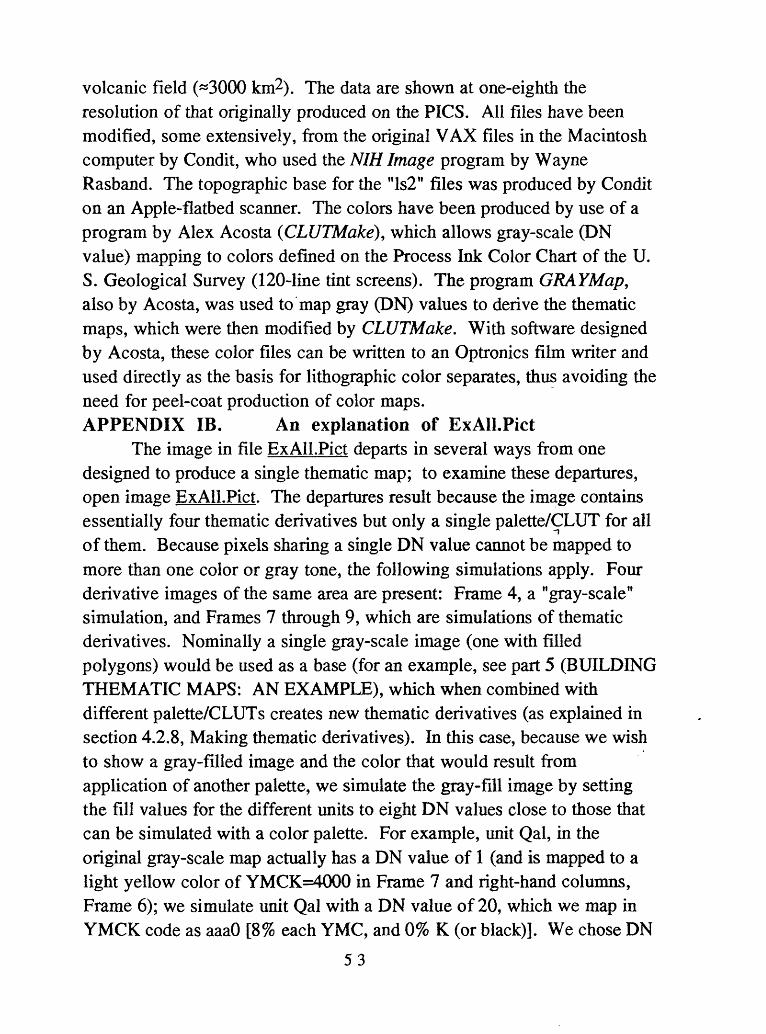
volcanic field («3000 km2). The data are shown at one-eighth the resolution of that originally produced on the PICS. All files have been modified, some extensively, from the original VAX files in the Macintosh computer by Condit, who used the NIH Image program by Wayne Rasband. The topographic base for the "Is2" files was produced by Condit on an Apple-flatbed scanner. The colors have been produced by use of a program by Alex Acosta (CLUTMake), which allows gray-scale (DN value) mapping to colors defined on the Process Ink Color Chart of the U. S. Geological Survey (120-line tint screens). The program GRAYMap, also by Acosta, was used to map gray (DN) values to derive the thematic maps, which were then modified by CLUTMake. With software designed by Acosta, these color files can be written to an Optronics film writer and used directly as the basis for lithographic color separates, thus avoiding the need for peel-coat production of color maps. APPENDIX IB. An explanation of ExAILPict

The image in file ExAILPict departs in several ways from one designed to produce a single thematic map; to examine these departures, open image ExAILPict. The departures result because the image contains essentially four thematic derivatives but only a single palette/CLUT for all of them. Because pixels sharing a single DN value cannot be mapped to more than one color or gray tone, the following simulations apply. Four derivative images of the same area are present: Frame 4, a "gray-scale" simulation, and Frames 7 through 9, which are simulations of thematic derivatives. Nominally a single gray-scale image (one with filled polygons) would be used as a base (for an example, see part 5 (BUILDING THEMATIC MAPS: AN EXAMPLE), which when combined with different palette/CLUTs creates new thematic derivatives (as explained in section 4,2.8, Making thematic derivatives). In this case, because we wish to show a gray-filled image and the color that would result from application of another palette, we simulate the gray-fill image by setting the fill values for the different units to eight DN values close to those that can be simulated with a color palette. For example, unit Qal, in the original gray-scale map actually has a DN value of 1 (and is mapped to a light yellow color of YMCK=4000 in Frame 7 and right-hand columns, Frame 6); we simulate unit Qal with a DN value of 20, which we map hi YMCK code as aaaO [8% each YMC, and 0% K (or black)]. We chose DN

53

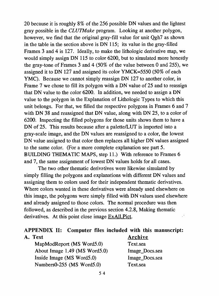
20 because it is roughly 8% of the 256 possible DN values and the lightest gray possible in the CLUTMake program. Looking at another polygon, however, we find that the original gray-fill value for unit Qgh7 as shown in the table in the section above is DN 115; its value in the gray-filled Frames 3 and 4 is 127. Ideally, to make the lithologic derivative map, we would simply assign DN 115 to color 6200, but to simulated more honestly the gray-tone of Frames 3 and 4 (50% of the value between 0 and 255), we assigned it to DN 127 and assigned its color YMCK=5550 (50% of each YMC). Because we cannot simply reassign DN 127 to another color, in Frame 7 we chose to fill its polygon with a DN value of 25 and to reassign that DN value to the color 6200. In addition, we needed to assign a DN value to the polygon in the Explanation of Lithologic Types to which this unit belongs. For that, we filled the respective polygons in Frames 6 and 7 with DN 38 and reassigned that DN value, along with DN 25, to a color of 6200. Inspecting the filled polygons for those units shows them to have a DN of 25. This results because after a palette/LUT is imported into a gray-scale image, and the DN values are reassigned to a color, the lowest DN value assigned to that color then replaces all higher DN values assigned to the same color. (For a more complete explanation see part 5. BUILDING THEMATIC MAPS, step 11.) With reference to Frames 6 and 7, the same assignment of lowest DN values holds for all cases.

The two other thematic derivatives were likewise simulated by simply filling the polygons and explanations with different DN values and assigning them to colors used for their independent thematic derivatives. Where colors wanted in these derivatives were already used elsewhere on this image, the polygons were simply filled with DN values used elsewhere and already assigned to those colors. The normal procedure was then followed, as described in the previous section 4.2.8, Making thematic derivatives. At this point close image ExAll.Pict.

APPENDIX II: Computer files included with this manuscript: A. Text Archive

MapModReport (MS Word5.0) Text.sea About Image 1.49 (MS Word5.0) Image_Docs.sea Inside Image (MS Word5.0) Image_Docs.sea NumbersO-255 (MS Word5.0) Textsea

54

Image Macros B. Programs

NIHImage CLUTMake GRAYMap

C. NIH Images (in Pict format,Active Image Window Figurel-5/30/93 ExAll.Pict SVFCSWls2Lith 253s47.PictSm ExTopo253 ExFilling Grays256,Pict ExFill ExTopo254 ExContExFillTopoContLabels 253s47&LineWk USGSCC-***.Pict (see below) ExAllGray.Pict SVFC-A-Fill SVFC-B-Topo SVFC-C-Contacts SVFC-D-LabelsAll Lithlnset SVFC-E-BGL

DN-CLUTBldMapLITH.PictInsetChemDN-CLUTBldMapChem.PictInsetPMagDN-CLUTBldMapPMag.PictThemelmageAThemelmageBSVFElsSFill SVFClsSFill

Text, sea

Imagel.49.sea ClutMake_GrayMap.sea ClutMake_GrayMap.sea

listed by order of use)NIHImageFiles.seaNIHImageFiles.seaNIHImageFiles.seaNIHImageFiles.seaNIHImageFiles.seaNIHImageFiles.seaNIHImageFiles.seaNIHImageFiles. seaNIHImageFiles.seaNIHImageFiles.seaNIHImageFiles.seaNIHImageFiles. seaNIHImageFiles.seaSee F. belowNIHImageFiles.seaBuildMap.seaBuildMap.seaBuildMap.seaBuildMap.seaBuildMap.seaBuildMap.seaBuildMap.sea BuildMap.sea BuildMap.sea BuildMap.seaBuildMap.seaNIHImageFiles.seaNIHImageFiles.seaNIHImageFiles.sea NIHImageFiles.sea

55

SVFWlsSFill SVFClsl6CQNTSVFClsl6FILLSVFClsl6FILLCQNTSVFElsl6CONTSVFElsl6FILLSVFElsl6FILLCONTSVFWlsl6CONTSVFWlsl6FILLSVFWsl6FILLCONTSVFlsl6TemplateSVFlsl6LithOverlaySVFlsl6ChemOverlaySVFlsl6PMagOverlayBLG-Clsl6REGISTRBLG-EM6REGISTRBLG-Wlsl6REGISTR

D.DNMAP files (ASCII format)ExMasterV3a.DNMAP SVFCLith.GrayDNMAP SVFELith.GrayDNMAP SVFWLith.GrayDNMAP SVFAllLithuDNMAP SVFAllChem.DNMAP SVFAllPMag.DNMAP SVFCChem.GrayDNMAP SVFEChem.GrayDNMAP SVFWChem.GrayDNMAP SVFCPMag.GrayDNMAP SVFEPMag.GrayDNMAP SVFWPMag.GrayDNMAP ThemeLith.DNMap ThemePMag.DNMap

E. GLUTS (palettes)SVFWPMag.GrayLUT ExMasterV3a.CLUT

NIHImageFiles.sea NIHImageFiles.sea NIHImageFiles.sea NIHImageFiles.sea NIHImageFiles.sea NIHImageFiles.sea NIHImageFiles.sea NIHImageFiles.sea NIHImageFiles.sea NIHImageFiles.sea NIHImageFiles.sea NIHImageFiles.sea NIHImageFiles.sea NIHImageFiles.sea NIHImageFiles.sea NIHImageFiles.sea NIHImageFiles.sea

DNMapFiles.sea DNMapFiles.sea DNMapFiles.sea DNMapFiles.sea DNMapFiles.sea DNMapFiles.sea DNMapFiles.sea DNMapFiles.sea DNMapFiles.sea DNMapFiles.sea DNMapFiles.sea DNMapFiles.sea DNMapFiles.sea DNMapFiles.sea DNMapFiles.sea

CLUTFiles.sea

56

CLUT-BldMapLith CLUT-BldMapChem CLUT-BldMapPMag ThemeLith.CLUT ThemePMag.CLUT SVFAllLithuCLUT SVFAllChem.CLUT SVFAllPMag.CLUT SVFCChemGrayLUT SVFCLith.GrayLUT SVFCPMag.GrayLUT SVFEChem.GrayLUT SVFELith.GrayLUT SVFEPMag.GrayLUT SVFWChem.GrayLUT SVFWLith.GrayLUT

F. USGS Color Code (Image) Files USGSCC-YMa%C.Pict USGSCC-YM13%C.Pict USGSCC-YM20%C.Pict USGSCC-YM30%C.Pict USGSCC-YM40%C.Pict USGSCC-YM50%C.Pict USGSCC-YM60%C.Pict USGSCC-YM70%C.Pict USGSCC-YMx%C.Pict USGSCC-YM.Pict USGSCC-YC.Pict USGSCC-MC.Pict

BuildMap.seaBuildMap.seaBuildMap.seaCLUTFiles.seaCLUTFiles.seaCLUTFiles.seaCLUTFiles.seaCLUTFiles.seaGrayLUTs.seaGrayLUTs.seaGrayLUTs.seaGrayLUTs.seaGrayLUTs.seaGrayLUTs.seaGrayLUTs.seaGrayLUTs.sea

USGSColoiCodes.sea USGSColoiCodes.sea USGSColorCodes.sea USGSColoiCodes.sea USGSColoiCodes.sea USGSColoiCodes.sea USGSColoiCodes.sea USGSColoiCodes.sea USGSColoiCodes.sea USGSColorCodes.sea USGSColorCodes.sea USGSColorCodes.sea

57

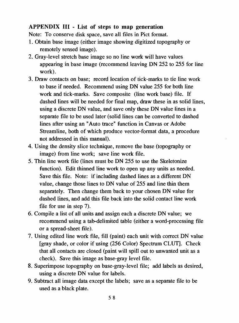
APPENDIX III - List of steps to map generationNote: To conserve disk space, save all files in Pict format.1. Obtain base image (either image showing digitized topography or

remotely sensed image).2. Gray-level stretch base image so no line work will have values

appearing in base image (recommend leaving DN 252 to 255 for line work).

3. Draw contacts on base; record location of tick-marks to tie line work to base if needed. Recommend using DN value 255 for both line work and tick-marks. Save composite (line work base) file. If dashed lines will be needed for final map, draw these in as solid lines, using a discrete DN value, and save only these DN value lines in a separate file to be used later (solid lines can be converted to dashed lines after using an "Auto trace" function in Canvas or Adobe Streamline, both of which produce vector-format data, a procedure not addressed in this manual).

4. Using the density slice technique, remove the base (topography or image) from line work; save line work file.

5. Thin line work file (lines must be DN 255 to use the Skeletonize function). Edit thinned line work to open up any units as needed. Save this file. Note: if including dashed lines as a different DN value, change those lines to DN value of 255 and line thin them separately. Then change them back to your chosen DN value for dashed lines, and add this file back into the solid contact line work file for use in step 7).

6. Compile a list of all units and assign each a discrete DN value; werecommend using a tab-delimited table (either a word-processing file or a spread-sheet file).

7. Using edited line work file, fill (paint) each unit with correct DN value [gray shade, or color if using (256 Color) Spectrum CLUTj. Check that all contacts are closed (paint will spill out to unwanted unit as a check). Save this image as base-gray level file.

8. Superimpose topography on base-gray-level file; add labels as desired, using a discrete DN value for labels.

9. Subtract all image data except the labels; save as a separate file to be used as a black plate.

58

10. Choose YMCK code for colors from USGSCC* files. Note: if using dashed contacts, reserve a color for those lines!

11. Using your table of DN values assigned to units, group the DN values you wish to send to common colors. Sorting on a column which has the attribute for that thematic map, using, for example, MS Word, facilitates this.

12. Make ASCII data-input file for CLUTMake and run CLUTMake using ASCII input file to create palette to import into your final map file.

13. In the following order combine (using the Replace option from the Paste Control Window) files together: a) Base-level gray file, b) topographic base file, c) line work file, and d) label file(s).

14. Import CLUT into this composite file.15. Create insets for map, and add in where desired.16. Set scale if needed.

59