URBP 204A QUANTITATIVE METHODS IStatistical Analysis Lecture I

Gregory NewmarkSan Jose State University

(This lecture accords with Chapters 2 & 3 of Neil Salkind’sStatistics for People who (Think They) Hate Statistics)

Descriptive Statistics• Statistics that describe a data set• Measures of Central Tendency – Mean (Average)– Median (Midpoint)– Mode (Most Prevalent)

• Measures of Variability– Range (Highest Value – Lowest Value)– Standard Deviation (Average Distance from Mean)– Variance (Average Distance from Mean Squared)

Central Tendency• What is the central tendency?– Single number that best describes data set– Representative score in a set of scores– Possible measures: Mean, Median, Mode

Mean (Average)• Mean – Average value– Sum of all values divided by the number of values

• What is the average housing value here?– Ms. Johnson’s House $600,000– Mr. Wood’s House $400,000– Ms. Brown’s House $500,000

Mean (Average)• Mean = ($600,000 + $400,000 +$500,000)/3

= $1,500,000/3= $500,000

• The average house value here is $500,000

• Problem: Mean is sensitive to extreme values• “If Bill Gates walked into this classroom, on

average, we would all be billionaires”

Mean (Average)• What is the average housing value here?– Ms. Johnson’s House + Addition $2,400,000– Mr. Wood’s House $400,000– Ms. Brown’s House $500,000

• Mean = ($2,400,000 + $400,000 +$500,000)/3 = $3,300,000/3

= $1,100,000• The average house value here is $1,100,000• Mean may no longer be a useful statistic

Median (Midpoint)• Median– Midpoint value (half above, half below)

• What is the median housing value here?– Ms. Johnson’s Mansion $2,400,000– Mr. Wood’s House $400,000– Ms. Brown’s House $500,000

Median (Midpoint)• To find the median:– Order the values [2,400,000; 500,000; 400,000]– Select the midpoint value [500,000]

• (If there are an even number of values, average the two middle values)

• Ms. Johnson’s addition is destroyed by a meteor and her house is worth $600,000 again.– What would the new median housing value be?

Median (Midpoint)• What does this map tell us?

Median vs. Mean

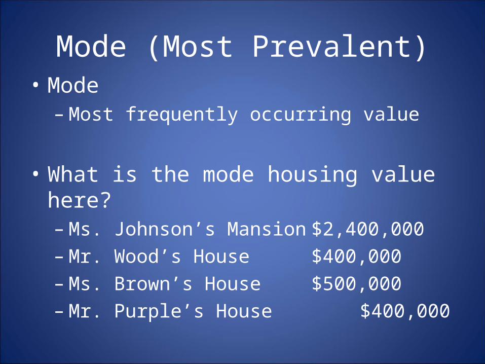
Mode (Most Prevalent)• Mode– Most frequently occurring value

• What is the mode housing value here?– Ms. Johnson’s Mansion $2,400,000– Mr. Wood’s House $400,000– Ms. Brown’s House $500,000– Mr. Purple’s House $400,000

Mode (Most Prevalent)• To find the mode– Count the frequencies of each value• 2,400,000 Once• 500,000 Once• 400,000 Twice

– Select the value with the highest frequency [400,000]

Mode (Most Prevalent)• The mode is very important with nominal data– Most voted for candidate– Most purchased beverage– Most common birth month– Favorite sports team– Most occurring M&M type

• Multimodalism? – If I ate all the red M&Ms, then what would the

new mode be?

When do I use which Measure?• Use the Mean when:– Values are interval or ratio measures– No values are extreme

• Use the Median when:– Values are interval or ratio measures– Some values are extreme

• Use the Mode when:– Values are nominal or ordinal measures

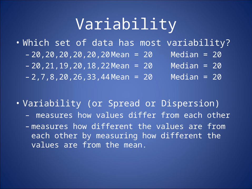
Variability• Which set of data has most variability?– 20,20,20,20,20,20 Mean = 20 Median = 20– 20,21,19,20,18,22 Mean = 20 Median = 20– 2,7,8,20,26,33,44 Mean = 20 Median = 20

• Variability (or Spread or Dispersion)– measures how values differ from each other– measures how different the values are from each

other by measuring how different the values are from the mean.

Range• Range = Highest Value – Lowest Value• What are the ranges for the following sets?– 20,20,20,20,20,20 Range = 20 - 20 = 0– 20,21,19,20,18,22 Range = 22 – 18 = 4– 2,7,8,20,26,33,44 Range = 44 – 2 = 42

Standard Deviation• Standard Deviation– Average distance from the mean– Sometimes called “mean error”– Like the mean, the SD is sensitive to extreme

values– Expressed in the same units as the underlying

values (the following examples are made up)• Mean Male Height: 5’10” with an SD of 3”• Mean TV Winnings: $4,760 with an SD of $3,400• Mean Runs per Game: 7.8 runs with an SD of 3.2 runs

– An SD of zero implies no variability

Standard Deviation• Standard Deviation (σ) – Average distance from the mean– Example• Mean = 50• SD = 20

Standard Deviation

Standard Deviation• Formula

Where s is the standard deviationΣ is sigma, which sums what followsX is each individual scoreXbar is the mean of all the scoresn is the sample size

Standard Deviation• Formula

“This formula finds the difference between each individual score and the mean (X – Xbar), squares each difference, and sums them all together. Then, it divides the sum by the size of the sample (minus 1) and takes the square root of the result.” (Salkind 2004)

Standard Deviation• Formula

• Why do we square the differences?• Why do we take the square root of everything?• Why do we minus 1 from n?

Standard Deviation• Why ‘n – 1’ and not just ‘n’:– This makes the resulting SD slightly larger– This is a conservative approach to apply the SD

from a sample to an entire population– Unbiased Estimate (versus the Biased Estimate)– As n grows, the unbiased estimated approaches

the biased estimate

Standard Deviation• Example– Runs scored by A’s in last nine games:• Runs: 3,3,4,5,5,7,8,9,10

– Formula

SD of A’s Runs ExampleGames Runs Average (X – Xbar) (X – Xbar)2 Last Steps

1 3 6 -3 9

2 3 6 -3 9

3 4 6 -2 4

4 5 6 -1 1

5 5 6 -1 1

6 7 6 1 1

7 8 6 2 4

8 9 6 3 9

9 10 6 4 16

Sum 54 0 54 54/(n-1) = 54/8 = 6.75

Square Root of 6.75 = 2.6

SD 2.6 Runs

Standard Deviation• Example:– Two curves with same μ but different σ– What does this say about the dispersion?

Variance• Variance = (Standard Deviation)2

– Not in same unit as original scores– Will become very relevant later in the class

• Formula