1

Urbanization without Growth:

A not so uncommon Phenomenon

Marianne Fay* and Charlotte Opal**

* World Bank (MFAY@Worldbank.org); ** Oxford University.This paper was written while Charlotte Opal was a summer intern at the World Bank

We are grateful to Vernon Henderson for the use of his data base and for his suggestions; to Bill Easterlyand the participants of the macro brownbag lunch seminar at the World Bank for their comments; and toChristine Kessides for her support and interest. All remaining errors are ours. This research was supportedby the Transport, Water, and Urban Division of the World Bank.

2

Introduction

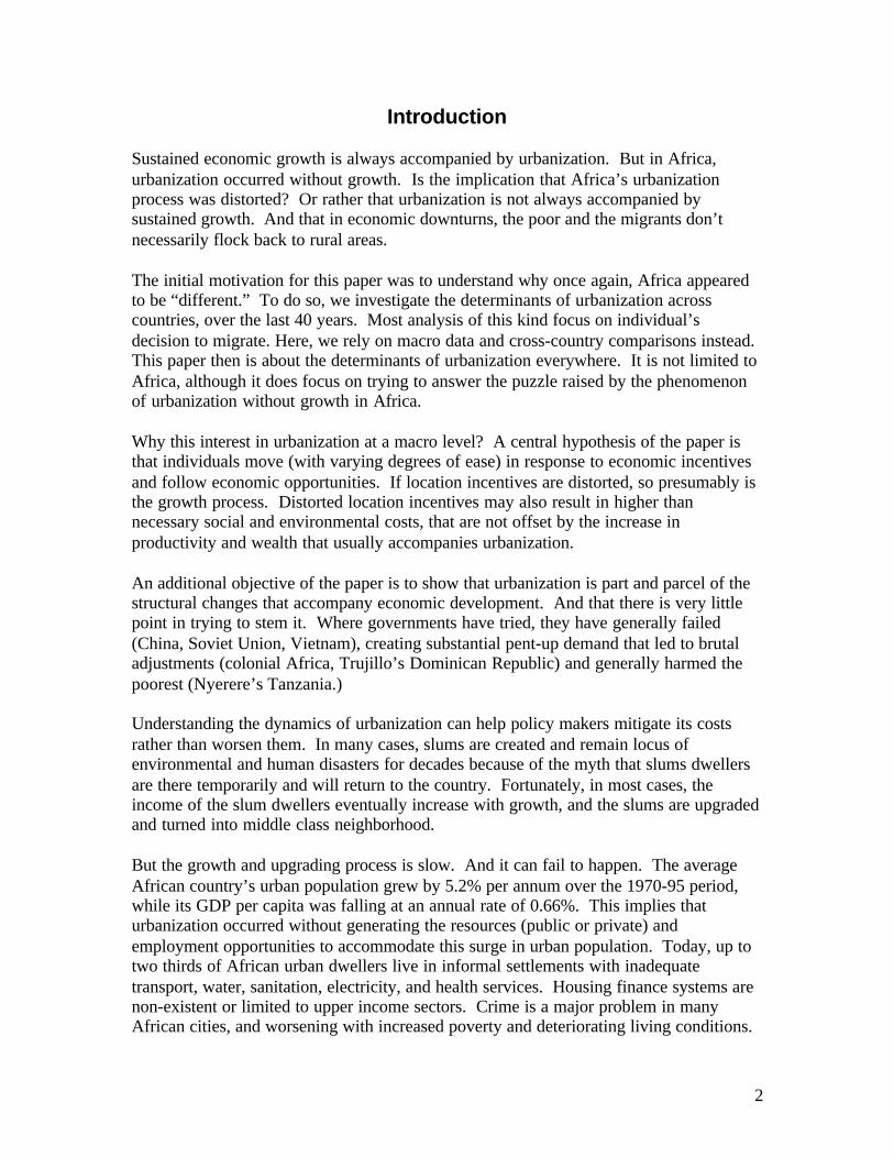
Sustained economic growth is always accompanied by urbanization. But in Africa,urbanization occurred without growth. Is the implication that Africa’s urbanizationprocess was distorted? Or rather that urbanization is not always accompanied bysustained growth. And that in economic downturns, the poor and the migrants don’tnecessarily flock back to rural areas.

The initial motivation for this paper was to understand why once again, Africa appearedto be “different.” To do so, we investigate the determinants of urbanization acrosscountries, over the last 40 years. Most analysis of this kind focus on individual’sdecision to migrate. Here, we rely on macro data and cross-country comparisons instead.This paper then is about the determinants of urbanization everywhere. It is not limited toAfrica, although it does focus on trying to answer the puzzle raised by the phenomenonof urbanization without growth in Africa.

Why this interest in urbanization at a macro level? A central hypothesis of the paper isthat individuals move (with varying degrees of ease) in response to economic incentivesand follow economic opportunities. If location incentives are distorted, so presumably isthe growth process. Distorted location incentives may also result in higher thannecessary social and environmental costs, that are not offset by the increase inproductivity and wealth that usually accompanies urbanization.

An additional objective of the paper is to show that urbanization is part and parcel of thestructural changes that accompany economic development. And that there is very littlepoint in trying to stem it. Where governments have tried, they have generally failed(China, Soviet Union, Vietnam), creating substantial pent-up demand that led to brutaladjustments (colonial Africa, Trujillo’s Dominican Republic) and generally harmed thepoorest (Nyerere’s Tanzania.)

Understanding the dynamics of urbanization can help policy makers mitigate its costsrather than worsen them. In many cases, slums are created and remain locus ofenvironmental and human disasters for decades because of the myth that slums dwellersare there temporarily and will return to the country. Fortunately, in most cases, theincome of the slum dwellers eventually increase with growth, and the slums are upgradedand turned into middle class neighborhood.

But the growth and upgrading process is slow. And it can fail to happen. The averageAfrican country’s urban population grew by 5.2% per annum over the 1970-95 period,while its GDP per capita was falling at an annual rate of 0.66%. This implies thaturbanization occurred without generating the resources (public or private) andemployment opportunities to accommodate this surge in urban population. Today, up totwo thirds of African urban dwellers live in informal settlements with inadequatetransport, water, sanitation, electricity, and health services. Housing finance systems arenon-existent or limited to upper income sectors. Crime is a major problem in manyAfrican cities, and worsening with increased poverty and deteriorating living conditions.

3

Unless economic growth accelerates substantially, there will be insufficient resources tofund the backlog of investments, let alone future requirements. Overstretched centralgovernments budgets are unlikely to suffice to fund the needed investments. Yetaccelerated growth is hampered by dysfunctional cities, which cannot service privatesector needs or provide markets for agricultural products.

The paper is organized as follows. The next section briefly looks at regional differencesin urbanization patterns, focussing on Africa. Part III offers a rapid review of theliterature on the determinants of urbanization. Part IV reports the results of testing thesehypothesis at the macro level and attempts to explain differences in levels of urbanizationacross countries while Part V looks at differences in the rate of growth of urbanizationacross countries. The last part concludes.

Throughout this paper, the expressions “overurbanized” or “underurbanized” are used.These expressions do not refer to deviation from an ideal level of urbanization. Rather,they are relative concepts, denoting differences from expected levels of urbanization,given sample norms. The level of urbanization is defined as the share of nationalpopulation residing in urban areas, Pu/P, where the definition of urban areas may varyacross countries. The rate of urbanization is the change in this level:

PPu

&&

where dots denote percentage change.

Africa’s urbanization in comparative perspective

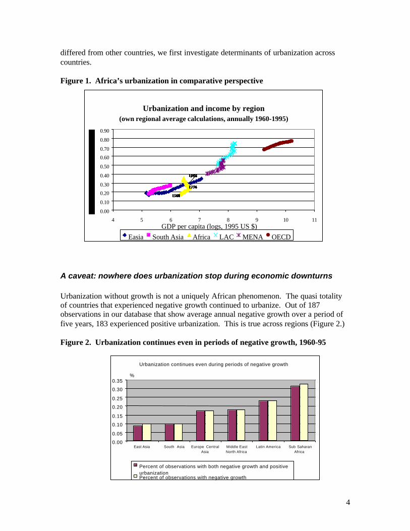
Africa emerged from the colonial period very underurbanized relative to its level ofincome. This was due, at least in part, to colonial regimes’ repression of rural-urbanmigration (Tarver, 1994). Africa in the early 1960s had about the same level ofurbanization as East and South Asia, although it was much wealthier (Figure 1.) Itsurbanization then proceeded along with income growth until the mid-70s. Africa thenentered a prolonged recession, while its population continued to flock to cities. Theresult is that today, Africa is relatively overurbanized given its income and economicstructure.1

Africa’s urbanization process was rapid, but appeared to follow a “normal” urbanizationpath until the mid-1970s. After about 1974, Africa diverged significantly from the worldtrend as it continued to urbanize more rapidly than other regions, even as its economieswere collapsing, or at least stagnating (Figure 1.) The question, then, is what caused thisphenomenon. Urban bias and distorted location policies? Civil war and agriculturalshocks which sent people to cities where aid was concentrated? Was it a cause or asymptom of what Easterly and Levine described as Africa’s growth tragedy (Easterly andLevine, 1997.) To determine whether -- or how -- Africa’s urbanization experience has

1 In 1995, 31% of Africa’s population was urban, but agriculture still employed 70% of its labor force. Incontrast, in South Asia 23% of the population resides in urban areas, but agriculture occupies only 62% ofthe labor force. Agriculture accounts for about 30% of GDP in both regions.

4

differed from other countries, we first investigate determinants of urbanization acrosscountries.

Figure 1. Africa’s urbanization in comparative perspective

A caveat: nowhere does urbanization stop during economic downturns

Urbanization without growth is not a uniquely African phenomenon. The quasi totalityof countries that experienced negative growth continued to urbanize. Out of 187observations in our database that show average annual negative growth over a period offive years, 183 experienced positive urbanization. This is true across regions (Figure 2.)

Figure 2. Urbanization continues even in periods of negative growth, 1960-95

Urbanization and income by region(own regional average calculations, annually 1960-1995)

0.00

0.10

0.20

0.30

0.40

0.50

0.60

0.70

0.80

0.90

4 5 6 7 8 9 10 11GDP per capita (logs, 1995 US $)

Easia South Asia Africa LAC MENA OECD

Urbanization continues even during periods of negative growth

0.00

0.05

0.10

0.15

0.20

0.25

0.30

0.35

East Asia South Asia Europe CentralAsia

Middle EastNorth Africa

Latin America Sub SaharanAfrica

%

Percent of observations with both negative growth and positiveurbanizationPercent of observations with negative growth

5

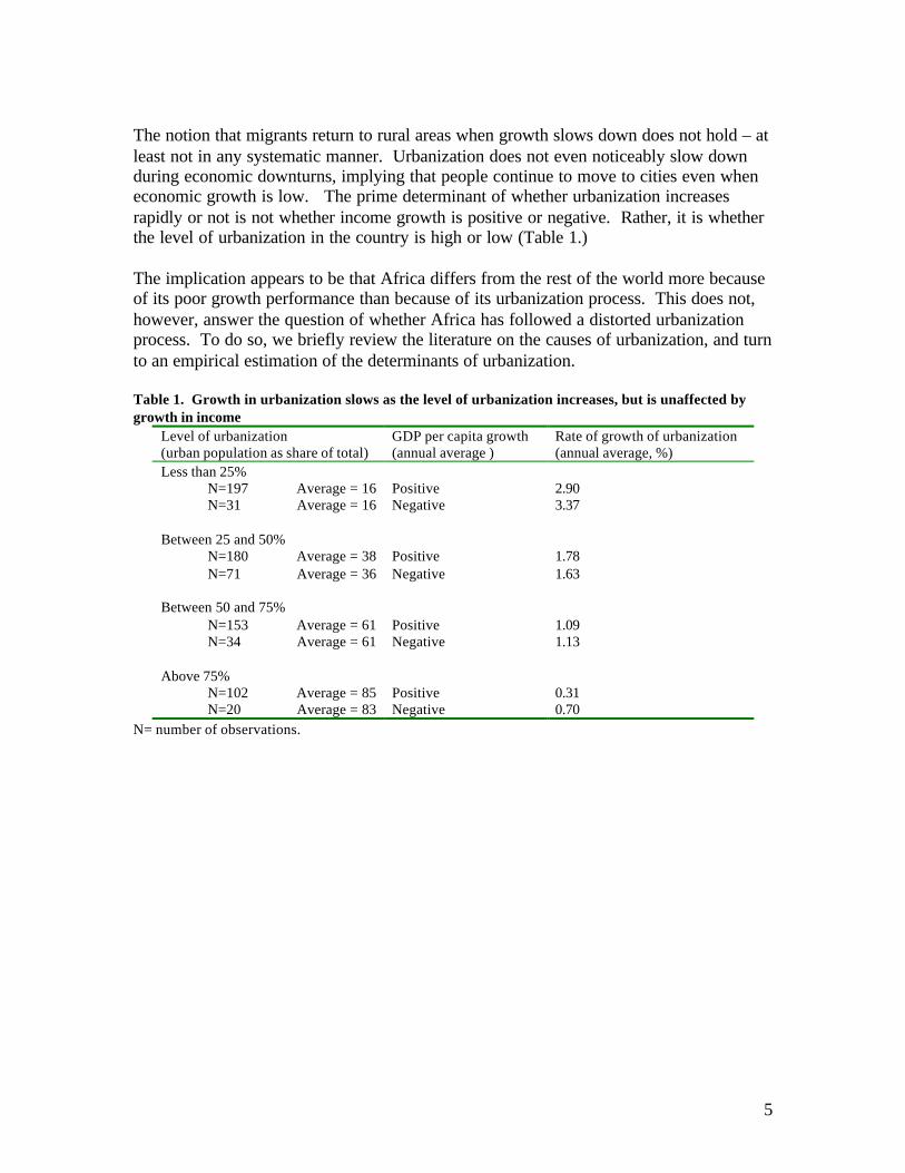
The notion that migrants return to rural areas when growth slows down does not hold – atleast not in any systematic manner. Urbanization does not even noticeably slow downduring economic downturns, implying that people continue to move to cities even wheneconomic growth is low. The prime determinant of whether urbanization increasesrapidly or not is not whether income growth is positive or negative. Rather, it is whetherthe level of urbanization in the country is high or low (Table 1.)

The implication appears to be that Africa differs from the rest of the world more becauseof its poor growth performance than because of its urbanization process. This does not,however, answer the question of whether Africa has followed a distorted urbanizationprocess. To do so, we briefly review the literature on the causes of urbanization, and turnto an empirical estimation of the determinants of urbanization.

Table 1. Growth in urbanization slows as the level of urbanization increases, but is unaffected bygrowth in income

Level of urbanization(urban population as share of total)

GDP per capita growth(annual average )

Rate of growth of urbanization(annual average, %)

Less than 25%N=197 Average = 16 Positive 2.90N=31 Average = 16 Negative 3.37

Between 25 and 50%N=180 Average = 38 Positive 1.78N=71 Average = 36 Negative 1.63

Between 50 and 75%N=153 Average = 61 Positive 1.09N=34 Average = 61 Negative 1.13

Above 75%N=102 Average = 85 Positive 0.31N=20 Average = 83 Negative 0.70

N= number of observations.

6

Causes of Rural-Urban Migration

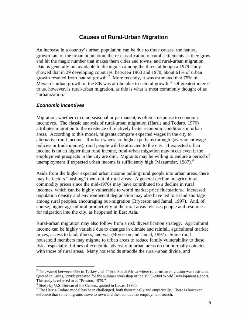
An increase in a country’s urban population can be due to three causes: the naturalgrowth rate of the urban population, the re-classification of rural settlements as they growand hit the magic number that makes them cities and towns, and rural-urban migration.Data is generally not available to distinguish among the three, although a 1979 studyshowed that in 29 developing countries, between 1960 and 1970, about 61% of urbangrowth resulted from natural growth. 2 More recently, it was estimated that 75% ofMexico’s urban growth in the 80s was attributable to natural growth. 3 Of greatest interestto us, however, is rural-urban migration, as this is what is most commonly thought of as“urbanization.”

Economic incentives

Migration, whether circular, seasonal or permanent, is often a response to economicincentives. The classic analysis of rural-urban migration (Harris and Todaro, 1970)attributes migration to the existence of relatively better economic conditions in urbanareas. According to this model, migrants compare expected wages in the city toalternative rural income. If urban wages are higher (perhaps through government wagepolicies or trade unions), rural people will be attracted to the city. If expected urbanincome is much higher than rural income, rural-urban migration may occur even if theemployment prospects in the city are dim. Migrants may be willing to endure a period ofunemployment if expected urban income is sufficiently high (Mazumdar, 1987).4

Aside from the higher expected urban income pulling rural people into urban areas, theremay be factors “pushing” them out of rural areas. A general decline in agriculturalcommodity prices since the mid-1970s may have contributed to a decline in ruralincomes, which can be highly vulnerable to world market price fluctuations. Increasedpopulation density and environmental degradation may also have led to a land shortageamong rural peoples, encouraging out-migration (Bryceson and Jamal, 1997). And, ofcourse, higher agricultural productivity in the rural areas releases people and resourcesfor migration into the city, as happened in East Asia.

Rural-urban migration may also follow from a risk diversification strategy. Agriculturalincome can be highly variable due to changes in climate and rainfall, agricultural marketprices, access to land, illness, and war (Bryceson and Jamal, 1997). Some ruralhousehold members may migrate to urban areas to reduce family vulnerability to theserisks, especially if times of economic adversity in urban areas do not normally coincidewith those of rural areas. Many households straddle the rural-urban divide, and

2 This varied between 38% in Turkey and 74% inSouth Africa where rural-urban migration was restricted.Quoted in Lucas, 1998b prepared for the summer workshop of the 1999-2000 World Development Report.The study is referred to as “Preston, 1979.”3 Study by U.S. Bureau of the Census, quoted in Lucas, 1998b4 The Harris-Todaro model has been challenged, both theoretically and empirically. There is howeverevidence that some migrants move to town and then conduct an employment search.

7

remittances between the rural household and migrants enable income smoothing (Lucas,1998b.)5

There is no systematic evidence showing that better services in urban areas(infrastructure, health clinics and schools) stimulates migration, although there isevidence that improved rural education triggers out-migration. As to better transport, itis unclear whether it stimulates migration, or encourages commuting and rural off-farmemployment (Lucas, 1998a)

Non-economic factors

Social and political conditions also play an important role in drawing people out of thecountryside into cities (Gugler and Flanagan, 1978). Migration to urban areas canprovide an escape from family and cultural constraints, such as restricted land access or alow level of female independence (Tacoli, 1998). Migration to an urban area may alsooccur because of an expected increase in social status and standing – the perception thatthe “high life” can be found among the “bright lights” of the city. 6 One study of northernGhanaian migrants to Accra revealed this powerful “bright lights” myth – migrants hadbeen lured to the city by exaggerated tales of high income and technologically advancedliving, especially by returned migrants who “wished to convey to others a positive imageof themselves and their experiences.” Migrants may also seek to acquire cash income tocontribute to bridewealth as the money economy increasingly penetrates marriage rituals(Gugler and Flanagan, 1978).

Wars and ethnic conflicts may also lead to an increase in rural-urban migration. Asidefrom the impact of war on agricultural income through effects on transport andmarketing, war may also push people out of rural areas for sheer safety reasons. Ethnicconflicts in particular increase the danger of living in an area dominated by a persecutedethnic group, as the potential for ethnic cleansing is high in these areas. Urban areasgenerally have a higher level of ethnic diversity and thus may be safe-havens forpersecuted groups. Police protection may also be higher in urban areas, encouragingmigration from war-torn rural areas where order may be more difficult to maintain.

Distorted location incentives: the infamous urban bias

Rural-urban wage differentials in the Harris-Todaro model reflect differences inproductivity that eventually disappear as a result of rural outmigration and themechanization of agriculture. But policy distortions may result in wage differentials inexcess of what is warranted by productivity. Alternatively, they may depress ruralproductivity or artificially inflate urban productivity for example through skewedinvestment allocations.

5 Note that resources can flow in both directions, and many migrant family will retain a foot in the ruralareas.6 According to Way, the process of urbanization has contributed to the HIV/AIDS pandemic in Africathrough this “bright lights” mechanism – populations which abandon their roots and head for the city havefrequently adopted “a lifestyle and behaviors that have placed them at increased risk for HIV infection”(435-6).

8

Jamal and Weeks (1998) attribute relatively higher urban wages in Africa to its colonialheritage. During the colonial era, higher urban wages represented a dichotomy between arich (European) governing class and a poor (African) agricultural class. Whencolonialism ended and an “Africanization” of urban jobs occurred, this wage gap wasmaintained. These relatively higher wages were often maintained by powerful tradeunions, which had been an important force in the achievement of independence and thuswere well organized and politically powerful. Wage laborers were often rewardedthrough favorable labor laws guaranteeing minimum wages and working conditions forgovernment workers, industrial employees, mineworkers, and other employees of theformal sector.

Developing country government investment may have been skewed towards urban-basedindustries during the 1960s and 1970s. The import-substitution strategies adopted bymany developing countries involved large-scale public works such as dams and roads,often financed by agricultural taxes (Jamal and Weeks, 1998). Michael Lipton’s 1977account of the flow of surplus from rural to urban areas in developing countries madefamous the notion of “urban bias.” This concept emphasized the price distortions presentin many developing countries that kept the price of rural agricultural products belowworld levels and the price of urban industrial products above world levels. Robert Batesin 1981 expanded the argument to attribute skewed investment in urban areas to therelative political power of urban dwellers, who could organize more easily and hadgreater access to government decision-makers. By influencing policy to increaseinvestment in urban infrastructure and industry, the urban elite could increase its incomeat the expense of rural agriculture (Tacoli, 1998). More recent evidence, however,suggests that cities –particularly large cities—subsidize the rest of the economy, at leastin terms of public expenditures and tax revenues (Prud’homme, 1998)

Private investment may also be skewed toward cities, through the existence of “financialurban bias.” Evidence from developing countries shows that urban areas tend to be netusers of credit, whereas rural areas tend to be net depositors – money is saved by peoplein rural areas but then borrowed by firms or individuals in urban areas (Chandavarkar,1985). This “financial urban bias” may exist because of a relatively higher degree ofcredit rationing in rural areas: transaction costs are high, monitoring is difficult, andaverage balances are small. The result may be a skewing of investment towards cities, ifmoney is saved in rural banks but lent through urban banks to be invested in urban firmsfor rates of return that are no higher than those that could be obtained in rural areas.

One important goal of the structural adjustment policies undertaken by developingcountries during the past two decades has been the reduction of these elements of “urbanbias,” by liberalizing agricultural commodity prices, realigning exchange rates, andreducing import barriers to force industrial products to compete internationally. Whetherbecause of general economic decline triggering falls in formal employment, or simplystructural adjustment reducing rents to an urban elite, Jamal and Weeks (1998) maintainthat, in Africa, “the income gap between urban wage earners and the rural population hasnarrowed considerably” since the mid-1970s. In fact, their study of four Africancountries found that “the primary dynamic distributional relationship in Africa has been

9

between rich and poor within both the urban and rural sectors,” rather than simplybetween rural and urban areas.

The phenomenon of “urban bias” may be better seen as a skewing of resource provisionto the rich and the elite, especially if the urban poor have limited access to theseresources. To equate people with their place of living denies the diversity in incomegroups among urban areas, and assumes that all urban dwellers benefit from policiesbiased towards urban groups. Thus it may be more appropriate to discuss “elite bias”rather than “urban bias” to take into account the economic differentiation among urbanpopulations.

Even if investment, credit, and fiscal and monetary policy primarily favor urban areas, itdoes not necessarily constitute an “urban bias.” It may reflect differentials in rates ofreturn. Furthermore, there may exists an optimal level of investment in which urbanareas receive relatively more infrastructure funding. If agglomeration economies exist ina certain industry, urbanization may increase productivity in that industry. Moregenerally, if urban credit and investment earn higher rates of return, it is more efficientfor credit to be concentrated in urban areas (Chandavarkar, 1985). The very process ofeconomic development implies disequilibria among rural and urban sectors, regions, andpopulations. Unequal resource allocation per capita is omnipresent in efficienteconomies, and may even be an impetus for economic development (Becker et al., 1994).

10

Explaining levels of urbanization across countries

Many economists and demographers have used the factors mentioned above to modelrural-urban migration. These models are usually probit-type models which attempt todetermine the probability of an individual agent deciding to move to an urban area from arural area. These models, therefore, look not only at the characteristics of the individual(culture, education, wealth, family support, etc), but also the individual’s environmentalfactors, both economic (rural-urban wage differential, returns to education, landavailability, etc) and social (the presence of violence in the rural areas, a lack of civilfreedoms).

Our study, however, focuses not on the individual, micro-economic level, but rather usesnational macroeconomic and social conditions to determine a country’s urbanizationprocess. We look at national urbanization levels and at changes in these urbanizationlevels, which to a large extent are the aggregate or the result of these individual migrationdecisions. Our focus remains Africa, but to be able to identify whether Africa isdifferent, we look across the world to see what has been the general experience withurbanization and economic development.

Figure 3. Urbanization and income,1960-857

U r b a n i s a t i o n a n d i n c o m e , 1 9 6 0 - 8 5 a l l c o u n t r i e s

0

10

20

30

40

50

60

70

80

90

100

0 2000 4 0 0 0 6 0 0 0 8000 10000 1 2 0 0 0 14000 16000 18000

Gdp per capita

% U

rban

Pop

ulat

ion

7 Data: Summers & Heston GDP; Urbanization: World Development Indicators. Based on Ingram, 1998.

11

The role of income

The share of a country’s population that resides in urban areas – that is, its level ofurbanization – is highly correlated with its level of per capita income. The share of urbanpopulation increases rapidly at low levels of income (and of urbanization) to converge toan urbanization level of about 80% (Figure 3). This transformation is due to thestructural changes that accompany development. The share of GDP derived fromagriculture falls from 32% among low income countries to less than 3% among rich ones,and the share of employment accounted for by agriculture falls by even more: from about66% to less than 6%.

Our basic model, therefore, is that urbanization is a function of income and incomesquared (to capture the non-linearity of the relationship),8 and of the structure of theeconomy:

U = E Ya + b ln Y (YA/Y) (YM/Y)which in logs yields:

u= e + a y + b y2 + c (yA-y) +d (yM-y)

In addition, we test the hypotheses mentioned above concerning rural-urban wagedifferentials, urban bias, rural “push” factors, civil disturbances and wars, and civil andpolitical rights. Our data is organized as an unbalanced panel data set, with observationsevery five years from 1965 to 1995, for up to 100 developed and developing countries.9

Regression 1 in Table 2 shows that income per capita, the share of GDP derived fromagriculture and manufacturing, and a time trend (“year”) explain 80% of cross countryvariations in levels of urbanization. 10 Because the variables are in logs, their coefficientsare elasticities. Thus a 10% increase in the share of GDP derived from manufacturingoccurs along with a 1.3% increase in the level of urbanization, while a 10% increase inthe share derived from agriculture coincides with a –1.3% decrease in the level ofurbanization.

Rural-urban differences in earnings

The literature on rural-urban migration discussed in the preceding sectionemphasizes the importance of rural-urban income differentials in explaining decisions tomigrate. No good measure of rural and urban wages was available, so we constructed onebased on average returns to labor. As a proxy for rural wages we used the averageproduct in agriculture, calculated simply as agricultural GDP (YA) divided by labor force

8 Since urbanization rates are bounded at 100%, the log-linear function is inadequate. We therefore use apolynomial to approximate the unknown function.9 Our database includes 1960, but because sectoral shares of GDP were not available for 1960, mostregressions omit that year.10 Manufacturing was used rather than industry because industry includes mining – an activity that wouldnot necessarily be correlated with the kinds of structural changes relevant to explaining urbanization.

12

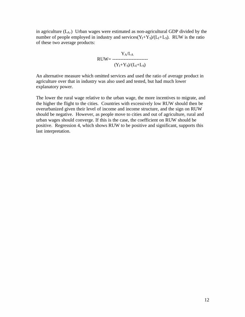
in agriculture (LA.) Urban wages were estimated as non-agricultural GDP divided by thenumber of people employed in industry and services(YI+YS)/(LI+LS). RUW is the ratioof these two average products:

YA/LARUW= ----------------------

(YI+YS)/(LI+LS)

An alternative measure which omitted services and used the ratio of average product inagriculture over that in industry was also used and tested, but had much lowerexplanatory power.

The lower the rural wage relative to the urban wage, the more incentives to migrate, andthe higher the flight to the cities. Countries with excessively low RUW should then beoverurbanized given their level of income and income structure, and the sign on RUWshould be negative. However, as people move to cities and out of agriculture, rural andurban wages should converge. If this is the case, the coefficient on RUW should bepositive. Regression 4, which shows RUW to be positive and significant, supports thislast interpretation.

13

Table 2: Explaining levels of urbanization

Regression 1 2 3 4 5 6 7 8 9 10 11Dates available 1965-95 1965-95 1965-95 1965-90 1965-90 1970-95 1965-95 1965-95 1965-90 1980-95 1965-90

Ln(Y) 1.46** 1.46** 1.73** 1.78** 1.91** 1.73** 1.79** 1.71** 1.80** 1.66** 2.06**(Ln (Y))2 -0.080** -0.080** -0.095** -0.10** -0.11** -0.096** -0.10** -0.095** -0.10** -0.090** -0.12**Ln (Yag/Y) -0.13** -0.13** -0.13** -0.22** -0.12** -0.14** -0.16** -0.15** -0.22** -0.10** -0.18**Ln(Ymanuf/Y) 0.13** 0.10** 0.11** 0.12** 0.15** 0.099** 0.12** 0.12** 0.11** 0.0084 0.19**Year 0.013** 0.013** 0.013** 0.0048 0Africa -0.028Africa*pre80 -0.19** 0.27 0.14 1.30** 0.44 0.28 0.21 0.22 0.677 1.29**Africa*post80 0.12** 1.66** 1.54** 2.01** 1.61** 1.95** 1.74** 1.61** 1.46** 2.28**Africa*pre80*ln(Y) -0.067 -0.031 -0.20** -0.091* -0.069 -0.062 -0.041 -0.12* -0.19**Africa*pre80*ln(Y) -0.24** -0.21** -0.29** -0.23** -0.28** -0.25** -0.22** -0.21** -0.32**post80 -0.031 -0.12** -0.12** -0.061Ln(Ruw) 0.18** 0.17** 0.15**Ln(Noeduc) -0.14** -0.17**(Ln(Noeduc))2 0.046** 0.055**Ln(secondary) 0.18** 0.14**Cereal 0.033**BMP 0.00016**Poscropsh 0.0049Negcropsh -0.0022Sivard 0.076** 0.076* 0.057*Ln(foodaidc) -0.031*Ln(foodaidnc) 0.084**

Adj. R2 .801 .813 .826 .855 .875 .822 .822 .816 .856 .802 .879N 494 494 494 398 352 437 450 494 398 331 346

The dependant variable is the log of the level of urbanization defined as (urban population/total population). Note: * (**) indicate significance at the 5% (10%) level.The sample is an unbalanced panel consisting of up to 100 countries every 5 years between 1965 and 1995. Results are robust to heteroscedasticity using White’smethod.

14

Education

We also expect education to be positively correlated with higher urbanization, as returnsto education tend to be higher in urban areas. Education itself may have an aspect of“urban bias”: rural students do not necessarily learn agricultural skills, and may even beeducated in such a way as to be averse to farming (Gugler and Flanagan, 1978). Usingeducation data from the Barro and Lee data set (Barro and Lee, 1996), we find inregression 5 that the higher the proportion of the population with no education, the lowerthe level of urbanization. This effect is non-linear however, as evidenced by the fact thatthe square of NOEDUC is positive and significant. The interpretation is simply thatamong countries with many uneducated people, a very small improvement in education isassociated with much higher urbanization. Conversely, among countries with relativelyfew uneducated people, improvements in education will basically not affect urbanization.

Other education variables are available from Barro and Lee, enabling us to distinguishamong different levels of educational achievements. However, they tend to be verycollinear. We therefore used only secondary education (SECONDARY), which yieldedthe best fit. It is positive and significant, suggesting that a typical country can expect tobe 12% more urbanized given its level of income and income structure than a countrywhose adult population has half the average years of secondary education.

Urban bias

No good measure of urban bias is readily available. In particular, it is impossible tomeasure whether public investment and spending is biased towards urban areas, due to alack of data and the difficulty of assessing which populations benefit from which publicinvestments. Two alternative measures can be used as proxies. One is the differencebetween the domestic producer price of agricultural products and their internationalmarket prices. These are available through the Food and Agriculture Organization of theUN for a number of basic products, notably cereals. If this functions as a measure ofurban bias, we expect a negative coefficient. But regression 6 shows CEREAL to besignificantly positive, implying that it is capturing a process of convergence, whereby themore urbanized a country, the closer to international prices is its domestic producer priceof agricultural commodities. CEREAL’s explanatory power, however, is low relative toincome or income structure.

Another measure of distortion which could presumably disproportionately affect ruralareas, or proxy for import substitution policies, is the overvaluation of the exchange rate.A common measure of this overvaluation is the ratio of the black market exchange rate tothe official rate, or the “black market premium” (BMP). We expect that, all elseconstant, countries with a higher black market premium should be more urbanized. Thisis indeed the case, as is shown in regression 7. To make sure that we were not simplycapturing a Latin American effect (Latin American countries are highly urbanized andmany had high black market premia in the eighties and early nineties), we ran regression7 with a Latin America dummy. The variable remained significantly positive. Its

15

explanatory power is trivial, however, and it is not significant when other explanatoryvariables, such as CEREAL, are introduced.

Shocks to agriculture

Another important factor which could “push” people out of rural areas is a shock toagricultural production. Agricultural shocks can include not only weather shocks such asdroughts – during one drought year in Mauritania, for instance, population in the capitalcity of Nouakchott doubled (Potts, 1995) – but also collapses in prices, disruptions in thedistribution system, or unavailability of fertilizers.

Rather than trying to create separate measures of these possible disruptions, weconstructed a variable that measures the difference between actual and expected cropoutput. POSCROPSH captures positive deviations (one or two standard deviations) fromexpected crop yield, while NEGCROPSH does the same for negative shocks to cropyield.11 We expect the sign on POSCROPSH to be positive (indicating that a better-than-expected crop yield over the previous 5 years will reduce the likelihood of a rural farmermoving to the city) and the sign on NEGCROPSH to be positive, as a bad yield wouldpush people into the city.

Neither NEGCROPSH nor POSCROPSH are significant (regression 8). However, wedid get expected results using annual shock measures (rather than the sum over thepreceding 5 years). This variable is highly sensitive to sample changes, however, and theresults were not always robust, so we did not include it in any of our summaryregressions. The Barro-Lee measure of terms of trade shocks (growth rate of exportprices minus growth rate of import prices averaged over the preceding 5-year period) wasnot significant in any of our regressions.

Civil disturbances, wars, and famines

As mentioned above, in times of civil strife, armed conflicts and large-scale atrocitiestend to occur away from the center of power ( battlefields are usually in the countryside.Mozambique and many other war-torn countries saw refugees flock to cities, usually themain city, which is also where relief efforts tend to be concentrated. Morrison’s 1993study of politically motivated violence and migration in Guatemala showed that evenwhen the number of deaths is relatively small, the “climate of fear” that these deathsinstill – particularly in rural residents – appears to have caused many individuals tomigrate.

11 These were calculated on an annual basis, with the variable given a value of 2 if the negative shock wasat least 2 standard deviations below expected, 1 if the shock was between 1 and 2 standard deviationsbelow expected, and 0 otherwise. NEGCROPSH is the sum of these over five years. It can therefore take avalue between 0, indicating no shocks in the previous five years, and 10 which would imply the countryexperienced severe negative shocks to crop yields every year in the past five years. POSCROPSH wascalculated using the same methodology. Expected yield was calculated using OLS estimates from aregression of actual yield on time.

16

We used two different measures of civil disturbance. One, which is used in Easterly andLevine (1997), is from Sivard (1996), who collects annual information on the numbers ofpeople killed because of civil conflict or war fought on the national territory. The other,food aid, more generally proxies for overall disturbances — economic or other.

The information collected in Sivard allowed us to test not only whether civil strife andurbanization were related, but also whether the impact on urbanization varied with theseverity of the domestic disturbances. We constructed three measures based on theinformation collected in Sivard: SIVARD, which indicates that the country wasmentioned in Sivard as having some form of civil strife; SIV1000, indicating that thecountry had more than 1000 deaths; and SIV5000, which were countries with more than5000 war-related deaths in the 5 preceding years.

Regression 9 shows that countries that experienced civil strife tend to be more urbanized,holding all other variables equal. The severity of the conflict does not appear to matter,as SIVARD yielded a better fit than SIV1000 or SIV5000.

The positive correlation between urbanization and civil strife is very sensitive to samplechanges, and is mostly driven by East Asian countries. Contrary to common perception,over the 1960-95 period, it is not in Africa that most civil strife occurred. Mentioned inSivard for some form of civil strife are 34% of the observations for East Asia, 24% forMiddle East and North Africa, and 20% each for Africa and Latin America. Theprolonged nature of civil unrest in countries such as Cambodia, Myanmar, and thePhilippines seems to have contributed to their urbanization.

Clearly, however, whether people seek refuge in cities may depend on the nature andstructure of the conflict. In Burundi, for example, people did move to Bujumbura toescape the risk of slaughter. In Rwanda, on the other hand, one group dominated Kigali,so that when refugees came back from Zaire, they tended to remain in the rural areas.Both these countries have experienced civil strife and war over prolonged periods oftime, yet remain among the two least urbanized countries in the world.

Our alternative measure of domestic hardships, food aid, is collected by the FAO. Itmeasures tons of cereal and non-cereal food aid received by a country. We expected bothmeasures (deflated by population) to be positively correlated with levels of urbanization,given that aid is probably more readily available in urban centers and that it is probablyreceived in times of famine (which would most likely be pushing people out of thecountryside). However, we find in regression 10 that cereal food aid (FOODAIDC) has anegative sign and that non-cereal food aid (FOODAIDNC) is positive. Both these resultsare very vulnerable to the introduction of other variables.

Ease of access to urban center

A basic elements in standard migration models is the ability of rural dwellers to move tourban areas, which is affected by the availability of transportation and the distance to thecity. To proxy ease of transportation we used road density, and for distance to urbancenters we used population density.

17

Road density was generally not significant, which may be due to the fact that while abetter road network does help people move to cities, it also means that the countryside isbetter integrated into the national economy so that rural dwellers can benefit from accessto urban markets without having to move to urban areas.

As to population density, its partial correlation coefficient is generally significantlynegative, which we cannot explain.12 Finally, work by Henderson suggests that ascountries start urbanizing, their urban systems tend to be very “primate” – that is,dominated by one main city. This is supported by our data, and we find higher primacy(defined as the percentage of urban dwellers who reside in the main city) is negativelycorrelated with urbanization. However, since this variable significantly reduces oursample, we did not include it in Table 2.

Democracy and urbanization

Non-democratic regimes with a large amount of cronyism and rent-seeking would beexpected to be relatively more urbanized, as people who wish to gain access to politicalfavors and rents concentrate their activities in the city (Ades and Glaeser, 1995). Also,dictatorships are vulnerable to riots and uprising – which are urban phenomena – andtherefore probably rely on public spending to keep the urban masses reasonably content.It should follow that non-democracies should be more urbanized given their level ofincome or other explanatory variables.

To test these hypotheses, we ran regression 11 on two separate samples, distinguishingbetween “democracies” and “non-democracies.” Non-democracies are countriesclassified as not free or only partially free by Freedom House, and democracies are thoseclassified as free. Regressions 12 and 13 in Table 3 show the results. The coefficients onincome, on the share of GDP derived from manufacturing, and on the education variablesare much higher in non-democratic countries. However, none of these differences isstatistically significant (that is, an interactive term between the democracy dummy andthese variables is never significant in regressions on the whole sample.) Nor did we findthe democracy variable to be significant when entered directly in a regression run on thewhole sample.

Barkley and McMillan (1994) argue that a lack of political and civil liberties can limitindividuals’ ability to respond to economic incentives. The government may restrain themovement of people and resources, or affect market information concerning relativereturns to resources, reducing reliance on the accuracy of economic indicators andmigration incentives.

12 Note that the simple correlation between urbanization and density is positive.

18

Table 3: Democracy and levels of urbanization

Regression 12 13 14non-democracies democracies Interaction

dates available 1975-95 1975-95 1975-95Ln(Y) 2.49** 1.62** 1.68**(Ln(Y))2 -0.15** -0.093** -.096**Ln (Yag/Y) -0.22** -0.20** -0.19**Ln(Ymanuf/Y) 0.34** -0.058 0.050Africa*pre80 1.65** -- droppeda -- 0.39Africa*post80 2.12** 2.93** 1.20**Africa*pre80*ln(Y) -0.23** -0.039** -0.073*Africa*pre80*ln(Y) -0.28** -0.44** -0.17**Ln(Noeduc) -1.51** -0.096**(Ln(Noeduc))2 0.27** 0.033**Ln(secondary) 0.17** 0.015Ln(RUW) 0.16** 0.32** 0.28**CivilRight*ln(RUW) -0.021**Sivard 0.018 0.093

Adj. R2 .875 .820 .851N 166 99 303

a. There were no countries classified as “Free” in Africa before 1980.Dependant variable is log of the level of urbanization. Notes: See Table 2.

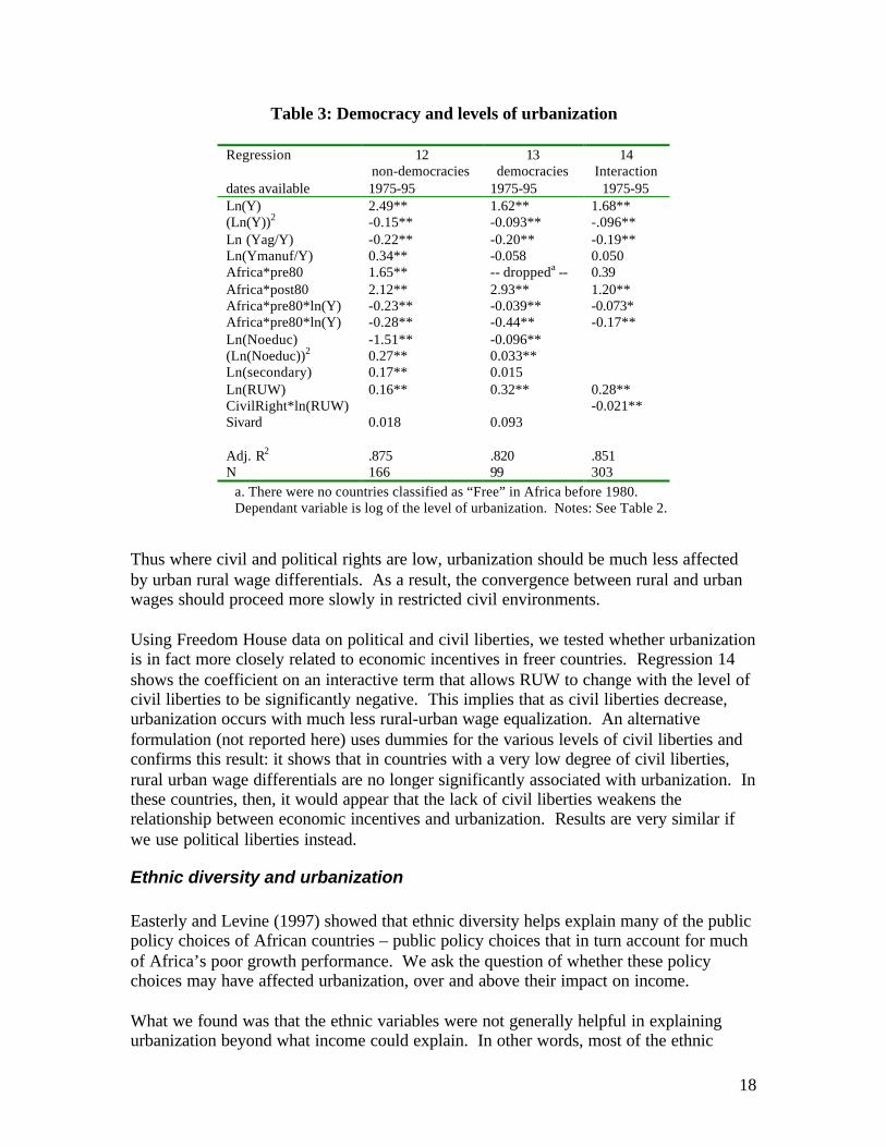
Thus where civil and political rights are low, urbanization should be much less affectedby urban rural wage differentials. As a result, the convergence between rural and urbanwages should proceed more slowly in restricted civil environments.

Using Freedom House data on political and civil liberties, we tested whether urbanizationis in fact more closely related to economic incentives in freer countries. Regression 14shows the coefficient on an interactive term that allows RUW to change with the level ofcivil liberties to be significantly negative. This implies that as civil liberties decrease,urbanization occurs with much less rural-urban wage equalization. An alternativeformulation (not reported here) uses dummies for the various levels of civil liberties andconfirms this result: it shows that in countries with a very low degree of civil liberties,rural urban wage differentials are no longer significantly associated with urbanization. Inthese countries, then, it would appear that the lack of civil liberties weakens therelationship between economic incentives and urbanization. Results are very similar ifwe use political liberties instead.

Ethnic diversity and urbanization

Easterly and Levine (1997) showed that ethnic diversity helps explain many of the publicpolicy choices of African countries – public policy choices that in turn account for muchof Africa’s poor growth performance. We ask the question of whether these policychoices may have affected urbanization, over and above their impact on income.

What we found was that the ethnic variables were not generally helpful in explainingurbanization beyond what income could explain. In other words, most of the ethnic

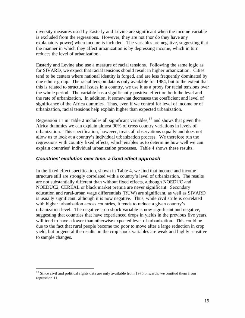
19

diversity measures used by Easterly and Levine are significant when the income variableis excluded from the regressions. However, they are not (nor do they have anyexplanatory power) when income is included. The variables are negative, suggesting thatthe manner in which they affect urbanization is by depressing income, which in turnreduces the level of urbanization.

Easterly and Levine also use a measure of racial tensions. Following the same logic asfor SIVARD, we expect that racial tensions should result in higher urbanization. Citiestend to be centers where national identity is forged, and are less frequently dominated byone ethnic group. The racial tension data is only available for 1984, but to the extent thatthis is related to structural issues in a country, we use it as a proxy for racial tensions overthe whole period. The variable has a significantly positive effect on both the level andthe rate of urbanization. In addition, it somewhat decreases the coefficient and level ofsignificance of the Africa dummies. Thus, even if we control for level of income or ofurbanization, racial tensions help explain higher than expected urbanization.

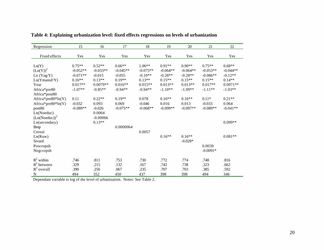
Regression 11 in Table 2 includes all significant variables,13 and shows that given theAfrica dummies we can explain almost 90% of cross country variations in levels ofurbanization. This specification, however, treats all observations equally and does notallow us to look at a country’s individual urbanization process. We therefore run theregressions with country fixed effects, which enables us to determine how well we canexplain countries’ individual urbanization processes. Table 4 shows these results.

Countries’ evolution over time: a fixed effect approach

In the fixed effect specification, shown in Table 4, we find that income and incomestructure still are strongly correlated with a country’s level of urbanization. The resultsare not substantially different than without fixed effects, although NOEDUC andNOEDUC2, CEREAL or black market premia are never significant. Secondaryeducation and rural-urban wage differentials (RUW) are significant, as well as SIVARDis usually significant, although it is now negative. Thus, while civil strife is correlatedwith higher urbanization across countries, it tends to reduce a given country’surbanization level. The negative crop shock variable is now significant and negative,suggesting that countries that have experienced drops in yields in the previous five years,will tend to have a lower than otherwise expected level of urbanization. This could bedue to the fact that rural people become too poor to move after a large reduction in cropyield, but in general the results on the crop shock variables are weak and highly sensitiveto sample changes.

13 Since civil and political rights data are only available from 1975 onwards, we omitted them fromregression 11.

20

Table 4: Explaining urbanization level: fixed effects regressions on levels of urbanization

Regression 15 16 17 18 19 20 21 22

Fixed effects Yes Yes Yes Yes Yes Yes Yes Yes

Ln(Y) 0.75** 0.52** 0.66** 1.06** 0.91** 0.90** 0.75** 0.68**(Ln(Y))2 -0.052** -0.033** -0.045** -0.075** -0.064** -0.064** -0.053** -0.044**Ln (Yag/Y) -0.071** -0.015 -0.055 -0.10** -0.28** -0.28** -0.086** -0.12**Ln(Ymanuf/Y) 0.16** 0.13** 0.19** 0.13** 0.15** 0.15** 0.15** 0.14**Year 0.017** 0.0079** 0.016** 0.015** 0.013** 0.013** 0.017** 0.0071**Africa*pre80 -1.07** -0.85** -0.94** -0.94** -1.10** -1.09** -1.11** -1.03**Africa*post80Africa*pre80*ln(Y) 0.11 0.22** 0.19** 0.078 0.16** 0.16** 0.11* 0.21**Africa*pre80*ln(Y) -0.032 0.093 0.069 -0.046 0.016 0.013 -0.033 0.064post80 -0.089** -0.026 -0.075** -0.068** -0.099** -0.097** -0.089** -0.041**Ln(Noeduc) 0.0064(Ln(Noeduc))2 -0.00066Ln(secondary) 0.13** 0.099**Bmp 0.0000064Cereal 0.0057Ln(Ruw) 0.16** 0.16** 0.081**Sivard -0.028*Poscropsh 0.0039Negcropsh -0.0091*

R2 within .746 .811 .753 .730 .772 .774 .748 .816R2 between .329 .215 .132 .167 .742 .738 .323 .662R2 overall .390 .256 .067 .235 .707 .703 .385 .592N 494 352 450 437 398 398 494 346Dependant variable is log of the level of urbanization. Notes: See Table 2.

21

So is Africa different?

The dummy for sub-Saharan Africa, in regression 1 (Table 2), is not significant, implying thatoverall, in the period 1965-1995, Africa’s level of urbanization was not significantly differentfrom that of other countries given its level of income and economic structure.14 We also testedour more specific hypothesis that Africa was relatively underurbanized prior to 1980, andoverurbanized thereafter. This theory supported by the data in regression 2: the coefficient onAfrica*pre80 is significantly negative and that on Africa*post80 significantly positive.

An interactive dummy was used (Africa*post80*ln(Y) and Africa*pre80*ln(Y)) to determinewhether the relationship between levels of income and urbanization was different in Africarelative to the rest of the world. Regression 3, which allows Africa to differ from the rest of theworld both in intercept and in slope, suggests that Africa was not in fact particularly uniqueprior to 1980. However, after 1980 this changed. Not only was urbanization relatively highamong African countries given their income and education levels (positive sign on theAfrica*post80 dummy), but differences in income began to explain less of the differences inurbanization.

Since we are in fact interested in African countries’ individual urbanization processes over time,the fixed effect specification is of greater interest. However, we cannot use the pre- and post-1980 Africa dummy with fixed effects, because we do not have a balanced panel. Table 4 istherefore of moderate use in helping us answer the question of whether Africa’s urbanizationwas different. Instead, we run a fixed-effect regression without the Africa dummy, and regressits residuals on the fixed-effects regression.

Table 5: Regression of Fixed Effect ResidualsRegression: 24 25Fixed effects Yes NoDependant variable Log of urbanization Residuals of regression 24ln(Y) 0.63** …(ln(Y))2 -0.04** ..Ln(Yag/Y) -0.02 ..Ln(Ymanuf/Y) 0.15** ..Year 0.018** ..Ln(noeduc) -0.002 ..(Ln(noeduc))2 0.017 ..Ln (secondary) 0.14** ..Post80 -0.01 ..Ln(RUW) 0.02 ..Africa*pre80 .. -0.29**Africa*post80 .. 0.33**Africa*pre80*ln(Y) .. 0.04**Africa*post80*ln(Y) .. -0.05**

R2 within 0.76 ..R2 between 0.72 ..R2 overall 0.65 0.12N 346 346Notes: See Table 2.

14 Note however that the Africa dummy is significant in the absence of variables on the structure of the economy.

22

Table 5 shows the results, leading us to conclude that Africa’s urbanization process was indeeddifferent from the world’s both before and after 1980. African countries were generallyunderurbanized prior to 1980, and urbanized faster than expected during the 1965-80 periodgiven their income level and structure, their levels of human capital, and their rural-urban wagedifferentials. This resulted in higher-than-expected levels of urbanization in the post 80 period.Following 1980, any change in income was associated with smaller changes in urbanizationlevel. None of the other explanatory variables help decrease the value or significance of theseAfrica dummies. The conclusion then does hold that Africa is different, but we cannot, withtraditional causes such as rural-urban income differentials or urban bias, explain why this is so.

Explaining changes in urbanization

The puzzle raised by Figure 1 is that Africa urbanized rapidly despite protracted negativegrowth. In fact, we find that in general the relationship between changes in urbanization andchanges in income is much weaker than the relationship between levels of income and levels ofurbanization. Variations in income and income squared alone explain 72% of the variation inurbanization levels, but growth in income explains only 5% of growth in urbanization, even ifwe disaggregate income growth into its rural and urban components.

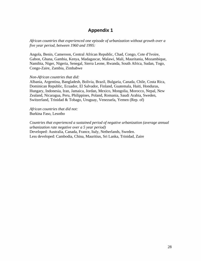
The generally weak relation between changes in income and in urbanization is due in part to thefact that rates of increase in urbanization are much more stable than rates of increase in income.Our sample means for the growth rate of income and urbanization are both 1.6% per annum, butthe minimum for urbanization is -0.9% while for income it is –11%.15 Negative urbanization isextremely rare. As shown in the Appendix, only 12 countries ever experienced decreases intheir levels of urbanization16. Finally, urbanization converges to 100% while income is (intheory at least) unbounded by any upper limit.

Nevertheless, we can “explain” a good part of the change in a country’s urbanization level. Firstand foremost, changes in urbanization are related to a country’s level of urbanization. This isshown in Table 6: U60, the level of urbanization in 1960, together with a time trend (year),explain about 55% of variations in the rate of urbanization across countries. ZY, the growth ratein income per capita, has no explanatory power whatsoever.

The Africa dummy shows that African countries did urbanize more rapidly than expected priorto 1980, and less rapidly after 1980. The fact that the AFRICA*PRE80 dummy is significant inregression 2 despite the fact that we correct for initial urbanization level, suggests that Africancountries where not simply “catching up”. Other policies or conditions were in place thatresulted in remarkably rapid urbanization during this period.

15 The maximum is about 12% for both. These numbers are for the larger sample of 630 countries. For the smallersample of 443 countries used in table 5 , the sample means are 1.5% for growth in urbanization (with a minimum of–0.8% and a maximum of 8.3%) and 1.2% for growth in income (varying between –7.5% and 7.8%.)16 Negative urbanization may have occurred in recent years in Eastern Europe and the former Soviet Union.

23

Table 6: Regressions in Changes in UrbanizationRegression 1 2 3 4dates available 1965-95 1965-95 1970-95 1970-95

ln(u60) -0.012** -0.012** -0.013** -0.012**year -0.00028** -0.00019** -0.00015** -0.00014**zy 0.016 00.015Africa 0.0011Africa*pre80 0.0043** 0.0036* 0.0035Africa*post80 -0.0026* -0.0052** -0.0051**zYags -0.023* -0.023*zYinds 0.016** 0.016**lagruw -0.0014*

Adj. R2 .549 .562 .603 .585N 630 630 443 437

Dependent variable is change in % urban population. Notes: see Table 2.

Since urbanization is thought to be associated with structural changes in the economy, weinclude terms for the share of growth derived from agriculture and from industry: ZYAGS andZYINDS.17 The share of growth in services was never significant, so we omitted it because itintroduced collinearity problems. As expected, we find that growth in agricultural value addedis associated with slower urbanization rates, while increases in industrial value added arepositively correlated with urbanization. The explanatory power of structural change variables issmall, however, as they only increase the R2 by about 1 percentage point. However, theirexplanatory power increases substantially when we exclude Africa from the sample (then theyadd about 4 percentage points to the R2.) Neither ZYAGS nor ZYINDS is significant in theAfrican sample.

We also test whether differences in rural and urban wages affect the speed of the urbanizationprocess. Since we want to establish the direction of causality, we used lagged values of RUW.The negative coefficient on LAGRUW confirms what most micro studies have found, namelythat low rural (relative to urban) wages contribute to rural-urban migration. In addition, theAFRICA*PRE80 dummy is generally not significant once LAGRUW is included in theregression. In other words, the speed of Africa’s urbanization prior to 1980 is no longer extra-ordinary if we take into account the very large disparities between urban and rural wages. InAfrica in 1970, the average product of labor in agriculture was only 15% of that in industry andservices. In South Asia and East Asia it was about 26%.

17 These are calculated as annual average growth in value added in agriculture and in industry, weighted by theirshares of GDP. They are not deflated by growth in population.

24

Table 7: Regressions in Changes

Regression 1 2 3 4 5 6 7 8dates available 1970-90 1975-95 1970-95 1970-95 1970-95 1975-95 1970-95 1975-95

ln(u60) -0.011** -0.012** -0.012** -0.012** -0.11** -0.011** -0.012** -0.012**year -0.00010 -0.00013** -0.00015** -0.00013** -0.00047 -0.00011* -0.00014** -0.00012*Africa*pre80 0.00077 0.0048** 0.0054** 0.0036 0.0023 0.0025 0.0031 0.0019Africa*post80 -0.0062** -0.0043** -0.0062** -0.0050** -0.0037** -0.0050** -0.0052** -0.0052**zYags -0.0085 -0.020 -0.023 -0.021 -0.0057 -0.011 -0.023* -0.012zYinds 0.012* 0.014** 0.20** 0.16** 0.012* 0.010 0.015** 0.0092lagruw -0.0011 -0.0018** -0.001 -0.0013 -0.0013* -0.0011 -0.0013* -0.0010cereal -0.000064bmp 0.0000006lag[ln(noeduc)] -0.00031lag[ln((noeduc)2)] 0.00011lag[ln(secondary)] -0.00083Poscropsh -0.00052Negcropsh 0.00022Sivard -0.0020* -0.0021*Democracy -0.0016* -0.0020**ln(foodaidc) -0.00043ln(foodaidnc) 0.00050

Adj. R2 .593 .603 .588 .589 .554 .580 .588 395N 368 412 382 432 329 395 437 .583

Dependent variable is change in % urban population. Notes: see Table 2..

25

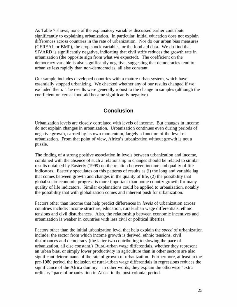
As Table 7 shows, none of the explanatory variables discussed earlier contributesignificantly to explaining urbanization. In particular, initial education does not explaindifferences across countries in the rate of urbanization. Nor do our urban bias measures(CEREAL or BMP), the crop shock variables, or the food aid data. We do find thatSIVARD is significantly negative, indicating that civil strife reduces the growth rate inurbanization (the opposite sign from what we expected). The coefficient on thedemocracy variable is also significantly negative, suggesting that democracies tend tourbanize less rapidly than non-democracies, all else constant.

Our sample includes developed countries with a mature urban system, which haveessentially stopped urbanizing. We checked whether any of our results changed if weexcluded them. The results were generally robust to the change in samples (although thecoefficient on cereal food-aid became significantly negative).

Conclusion

Urbanization levels are closely correlated with levels of income. But changes in incomedo not explain changes in urbanization. Urbanization continues even during periods ofnegative growth, carried by its own momentum, largely a function of the level ofurbanization. From that point of view, Africa’s urbanization without growth is not apuzzle.

The finding of a strong positive association in levels between urbanization and income,combined with the absence of such a relationship in changes should be related to similarresults obtained by Easterly (1999) on the relation between income and quality of lifeindicators. Easterly speculates on this patterns of results as (i) the long and variable lagthat comes between growth and changes in the quality of life, (2) the possibility thatglobal socio-economic progress is more important than home country growth for manyquality of life indicators. Similar explanations could be applied to urbanization, notablythe possibility that with globalization comes and inherent push for urbanization.

Factors other than income that help predict differences in levels of urbanization acrosscountries include: income structure, education, rural-urban wage differentials, ethnictensions and civil disturbances. Also, the relationship between economic incentives andurbanization is weaker in countries with less civil or political liberties.

Factors other than the initial urbanization level that help explain the speed of urbanizationinclude: the sector from which income growth is derived, ethnic tensions, civildisturbances and democracy (the latter two contributing to slowing the pace ofurbanization, all else constant.) Rural-urban wage differentials, whether they representan urban bias, or simply lower productivity in agriculture than in other sectors are alsosignificant determinants of the rate of growth of urbanization. Furthermore, at least in thepre-1980 period, the inclusion of rural-urban wage differentials in regressions reduces thesignificance of the Africa dummy – in other words, they explain the otherwise “extra-ordinary” pace of urbanization in Africa in the post-colonial period.

26

Our measures of urban bias (ratio of domestic to world price of cereals; black marketpremium) or of shocks to agriculture are never significant determinants of either the levelor the pace of urbanization. At any rate, they do not help explain why Africa is different.

One can question whether the particularly high rural-urban wage differentials in Africa inthe post-colonial period is a symptom of urban bias. It is possible, but by no meanscertain. They may have reflected differences in productivity – the fact that they graduallydecreased over time at about the same rhythm as in East and South Asia supports thishypothesis. Anyway, they are surely best understood as a symptom of elite – rather thanurban-- bias.

So does Africa’s urbanization process remain a puzzle? Africa, at the end of the colonialperiod, was underurbanized given its income and income structure due to the policies ofthe colonial powers. The 1960-80 period was characterized by very rapid urbanization,even more rapid than can be explained by a catch-up hypothesis, traditional urban-biasmeasures, agricultural shocks, or civil disturbances. It is largely explained, however, byrural-urban wage differentials. The slowdown in the pace of urbanization after 1980 issignificantly greater than can be explained by our explanatory variables. However, giventhat Africa had urbanized “exceedingly rapidly” in the 1960-80 period, the slowdown thatfollowed is not unexpected. In fact, if we let initial urbanization level take 1975 valuesfor the 1980-90 observations (instead of 1960), the post-80 Africa dummy is no longersignificant.

Alternative explanations could, of course, be poor data. One argument is thaturbanization data in Africa are simple projections based on old census data and thereforethe results presented here have limited meaning and interest. But if this were the case, weshould find that Africa in the post-80 period continued to urbanize exceedingly rapidly.The bias would be in the other direction. Another point frequently made is that we mayseverely underestimate income and income growth in Africa, as much of the economyhas gone underground to escape predatory governments. This point, while surelyaccurate,18 is moot because income growth explains so little of the pace of urbanization.

A more interesting criticism is that the distinctions between urban/rural andformal/informal may be misplaced in developing countries, especially in Africa. Manyworkers straddle these divisions, whether by seasonal or circular migration between townand country, or moonlighting in the informal sector while holding a formal sector jobduring the day (Jamal and Weeks, 1998). Even the economic activities we use todistinguish between rural and urban sectors may not be appropriate. The growth of urbanagriculture in response to rising food prices and shortages and general urban poverty is agood example of how strict rural vs. urban dichotomies may not be applicable to themodern developing world (Tacoli, 1998). This, however, is far from being a uniquelyAfrican phenomenon. In Nicaragua, 40% of the urban poor are employed in

18 The inclusion in Zaire’s national accounts of its “non-registered economy” raises “effective” GDP tothree times the current official measures of GDP (Cour, 1991.)

27

agriculture.19 Nevertheless, the very fact that our results show a weak relationshipbetween urbanization and traditionally accepted migration factors may indicate that, inAfrica at least, we are omitting part of the urbanization story. The fact that the informalsector provides a significant source of income to urban migrants, coupled with theapparent overlap of rural and urban activities, may shed light on the nature ofurbanization in Africa.

19 Nicaragua draft PRSP (http://www.mipres.gob.ni/grupoconsultivo)

28

Appendix 1

African countries that experienced one episode of urbanization without growth over afive year period, between 1960 and 1995:

Angola, Benin, Cameroon, Central African Republic, Chad, Congo, Cote d’Ivoire,Gabon, Ghana, Gambia, Kenya, Madagascar, Malawi, Mali, Mauritania, Mozambique,Namibia, Niger, Nigeria, Senegal, Sierra Leone, Rwanda, South Africa, Sudan, Togo,Congo-Zaire, Zambia, Zimbabwe

Non-African countries that did:Albania, Argentina, Bangladesh, Bolivia, Brazil, Bulgaria, Canada, Chile, Costa Rica,Dominican Republic, Ecuador, El Salvador, Finland, Guatemala, Haiti, Honduras,Hungary, Indonesia, Iran, Jamaica, Jordan, Mexico, Mongolia, Morocco, Nepal, NewZealand, Nicaragua, Peru, Philippines, Poland, Romania, Saudi Arabia, Sweden,Switzerland, Trinidad & Tobago, Uruguay, Venezuela, Yemen (Rep. of)

African countries that did not:Burkina Faso, Lesotho

Countries that experienced a sustained period of negative urbanization (average annualurbanization rate negative over a 5 year period)Developed: Australia, Canada, France, Italy, Netherlands, Sweden.Less developed: Cambodia, China, Mauritius, Sri Lanka, Trinidad, Zaire

29

Appendix 2Contrasting the experience of the world’s poor countries with that of Africa, 1960-

8520

Urbanisation and incomeNon African Poor countries, 1960-85

0

10

20

30

40

50

60

70

80

90

100

0 500 1000 1500 2000 2500 3000 3500 4000

GDP per capita

% U

rban

Pop

ulat

ion

Urbanisation and incomeAll African Countries, 1960-85

0

10

20

30

40

50

60

70

80

90

100

0 500 1000 1500 2000 2500 3000 3500 4000

GDP per capita

% U

rban

Pop

ulat

ion

Sth Africa

Gabon

20 Data: Summers & Heston GDP; Urbanization: World Development Indicators. Based on Ingram, 1998.

30

Bibliography

Ades, Alberto and Edward Glaeser. “Trade and Circuses: Explaining Urban Giants.”Quarterly Journal of Economics 110(1):195-258.

Barkley, Andrew P and John McMillan. “Political freedom and the response to economicincentives: Labor migration in Africa, 1972-1987.” Journal of Development Economics,Vol. 45 (1994), pages 393-406.

Becker, Charles M., Andrew M. Hamer, and Andrew R. Morrison. Beyond urban bias inAfrica. London: James Currey, 1994.

Bryceson, Deborah Faye and Vali Jamal. Farewell to Farms: De-agrarianisation andEmployment in Africa. Ashgate: 1997.

Chandavarkar, Anand G. “The Financial Pull of Urban Areas in LDCs.” Finance andDevelopment. June 1985, pages 24-27.

Cour, Jean-Marie. ____________. Villes en développement, Number 13, September,1991, Paris: Institut des Sciences et des Techniques de L’Equipement et del’Environnement pour le Développement.

Easterly, William. “Life during Growth.” Mimeo. The World bank. March 1999.

Easterly, William and Ross Levine. “Africa’s Growth Tragedy: Policies and EthnicDivisions.” Quarterly Journal of Economics, November 1997, pages 1205-1250.

Gugler, Josef and William G. Flanagan. Urbanization and social change in West Africa.Cambridge University Press, 1978.

Ingram, Gregory K. “Patterns of Metropolitan Developments: What Have We Learned?”Urban studies 35(7). 1998.

Jamal, Vali and John Weeks. “The vanishing rural-urban gap in sub-Saharan Africa.”International Labour Review. Vol. 127, No. 3, 1998, pages 271-292.

Lucas, Robert E.B. “Note on Internal Migration” prepared for the Summer Workshop ofthe 1999-2000 World Development Report, 1998a.

Lucas, Robert E.B. “Internal migration and urbanization: Recent contributions and newevidence.” Background Paper for the World Development Report 1999-2000, November1998b.

31

Mazumdar, Dipak. “Rural-urban migration in developing countries.” In Edwin S. Mills,ed. Handbook of regional and urban economics, Volume 2. Amsterdam: ElsevierScience Publishers, 1987.

Morrison, Andrew. “Violence or economics: What drives internal migration inGuatemala?” Economic Development and Cultural Change, Vol. 41, July 1993, pages817-831.

Potts, Deborah. “Shall we go home? Increasing poverty in African cities and migrationprocesses.” The Geographic Journal. Vol. 161, Part 3, November 1995, pages 245-264.

Prud’homme, Remy. “Note on urbanization” prepared for the Summer Workshop of the1999-2000 World Development Report, 1998.

Sivard, Ruth. World Military and Social Expenditures 1996. Washington, DC: WorldPriorities.

Tacoli, Cecilia. “Rural-urban interactions: A guide to the literature.” Environment andUrbanization. Vol. 10, No. 1, April 1998, pages 147-166.

Tarver, James D., Ed. “Urbanization in Africa: a Handbook.” London: Greenwood Press,1994.

Way, Peter O. “African HIV/AIDS and urbanization.” In James D. Tarver, ed.Urbanization in Africa. London: Greenwood Press, 1994, pages 423-438.

Weeks, John. “Economic aspects of rural-urban migration.” In James D. Tarver, ed.Urbanization in Africa. London: Greenwood Press, 1994, pages 388-407.

World Bank UserK:\Personal\urban paper\urbpprmay00 Vtables.doc05/09/00 9:22 PM