Urbanisation, Growth, and Development: Evidence

from India

Jonathan Colmer1

London School of Economics

Abstract

How does the spatial distribution of economic activity evolve as countries grow and de-velop, and what role does urbanisation play in this process? This paper examines thesequestions in the context of India, a country which, in spite of substantial economicgrowth, has experienced slow rates of urbanisation. We explore how India’s urban hi-erarchy and the spatial allocation of economic activity and resources have evolved overtime (1901–2011), and consider the consequences and importance of this process forgrowth and development. In addition, we examine and summarise the evidence on howgovernment policies, institutions, and public investments have influenced the spatial al-location of resources, how these factors affect welfare, growth, and development and,where questions remain, propose a research agenda for the future.

1 Introduction

Urbanisation is central to the development process; however, the welfare implications ofurbanisation, and its impact on growth and development are little understood. What de-termines the allocation of resources, people, and economic activity across space? Is thisallocation efficient? What role do institutions and public policy play in shaping this alloca-tion?

Between 1950 and 2010, the world’s urbanisation rate increased from just under 30% toover 50%. For the most part, this has been driven by developing countries such as Chinaand Korea, where urbanisation has accompanied substantial increases in income growth.However, we also observe substantial increases in the urbanisation rate in other countriesdespite persistent poverty and limited state capacity. This relationship is commonly observedin developing economies, where changes in income correlate only weakly with changes in therate of urbanisation. This suggests that policy and institutions may be an important driverin influencing the urbanisation process.

1The Centre for Economic Performance and the Grantham Research Institute, London School of Eco-nomics, Houghton Street, London WC2A 2AE, UK. E-mail: j.m.colmer@lse.ac.uk. I thank JeremiahDittmar, Vernon Henderson, and Guy Michaels for their thoughts, comments, and suggestions. I am grate-ful to Sam Asher, Somik Lall, and Hyoung Gun Wang for their assistance and advice with the data. Thisproject was supported by the Oxford University/LSE/World Bank Urbanisation in Developing EconomiesProgramme. All errors and omissions are my own.

1

This paper aims to understand the relationship between urbanisation, growth and devel-opment in the context of India, with a focus on presenting a series of stylised facts and, wherequestions remain, a research agenda for the future. India is a country where this relationshipis somewhat different: despite rapid economic growth, and substantial reductions in poverty,it has experienced languid rates of urbanisation. Urbanisation in India is currently less that30% of the population, having increased from 10% since independence.2 What explains thisslow demographic transition and what are the consequences for welfare and its continuingeconomic development?

India will soon have 20% of the world’s working-age population – a significant economicopportunity. At present, agriculture provides employment to around 220 million of India’s500 million workforce (Census, 2001). With an expected influx of an additional 250 millionworkers by 2030 it seems inevitable that growth in industry and services is a necessarycondition for future development (McKinsey, 2010). What are the constraints to furtherurbanisation and industrialisation in India, and how can these be relaxed to foster growthand take advantage of economic opportunities? Is industrialisation a necessary condition forurbanisation, or has the role of structural transformation from agriculture into manufacturingchanged? How does urbanisation affect spatial growth patterns across different sectors?

Unlike most developing countries, India’s urbanisation has been characterised by an un-usually large number of highly-populated cities. In 2001, 27.9% of the urban populationresided in 31 cities with a population of 1 million or more, compared with 9.5% of the urbanpopulation in 1911 (2 cities).3 Once all major cities (> 100,000 population) have been ac-counted for, 62% of the urban population reside in 441 towns and cities – 8% of total urbanareas. This results in a highly skewed composition of the urban population.

Are these mega-cities too large? Should policy makers focus resources on encouragingsmaller cities to grow, or invest in infrastructure to allow larger cities to better support urban-isation? In asking such questions one must consider why people live in cities to begin with.While there are many explanations, two stand out as being particularly relevant: economicagents live in cities because they enjoy it, and/or they can be more productive. Conse-quently, a combination of amenities and productivity levels determine city size; however, ascities grow, these benefits are offset by the costs and frictions associated with increased con-gestion. How fast the benefits of urban amenities and productivity deteriorate as cities growwill depend on institutional capacity and the quality of governance, as well as the degreeto which amenities and productivity effects are amplified by the presence of agglomeration

2The BRICS economies had urbanisation rates at 50% by the 1960s, the exceptions being China andIndia, where rates were between 10 and 20%. However, urbanisation increased rapidly following the CulturalRevolution in China, reaching nearly 50% of the population in 2010.

3These 31 cities account for less than 1% of the total number of urban towns and cities (5,176).

2

externalities.An additional characteristic of urbanisation in India is the degree of urban sprawl that is

observed. What are the welfare implications of urban sprawl? How does this decentralisa-tion affect economic activity? What are the costs of remoteness? It has been suggested thaturban sprawl in India is linked to a number of potentially distortive land use regulations,most notably vertical limits in the form of Floor Area Ratios (Bertaud, 2002; Bertaud andBrueckner, 2005; Brueckner and Sridhar, 2012; Glaeser, 2011; Sridhar, 2010; World Bank,2013) and the Urban Land Ceiling and Regulation Act of 1976, which is claimed to hin-der intra-urban land consolidation and restrict the supply of land available for developmentwithin cities (Srindhar, 2010). Urban sprawl is argued to increase the cost of intra-urbancommuting, affecting the range of jobs and services that are accessible within a city, as wellas the extent to which agglomeration externalities can be realised (Bertaud, 2004; Cervaro,2013; Harari, 2014). To the degree that this is true, the results from these studies indi-cate that policies to improve urban mobility, such as direct interventions in transportationinfrastructure, as well as the promotion of more compact development through land useregulations, could substantially improve welfare.

However, while reducing the costs of commuting, such interventions, may increase sprawl.Investments in transportation infrastructure within and around cities will cause them tospread out, reflecting an increase in the demand for space, cheaper labour and cheaperland on the urban fringe (See Redding and Turner (2015) for a review of the literature.)Furthermore, it is unclear a priori whether the premise that commuting costs are a first-order concern, is true. In the classical monocentric city model the city is made up of asingle central business district (CBD) surrounded by residential suburbs, where city dwellersmust commute to the CBD to earn income; however, while this model may be relevantfor certain sectors and may have been an accurate description of economic activity in thepast, the spatial concentration of economic activity has evolved in response to a number offactors: explicit policies, such as environmental regulation prohibiting polluting industrieswithin cities (Henderson, 1996; Greenstone, 2002); the life cycle of production (youngerindustries gain more from knowledge spillovers, which are enhanced by a greater geographicconcentration of economic activity (Desmet and Rossi-Hansberg, 2009)); and technologicalchange (improved access to transportation and information technology have substantiallyreduced communication costs, lowering the costs of decentralisation (Glaeser and Kahn, 2005;Duranton and Turner, 2012; Baum-Snow et al., 2014; Ghani et al., forthcoming; Khanna,2014;)). In this respect, urban sprawl may be, in part, a standard market response. Moreevidence is needed to understand the economic consequences of urban sprawl and its effectson, and relevance for, the spatial distribution of economic activity, growth, and development.

3

In considering all of these factors, it is important to bear in mind the general equilibriumnature of urbanisation. Investments or policy interventions to attenuate scale diseconomiesor amplify scale economies in one location may attract firms, workers and consumers fromother locations. Similarly, the economic consequences of negative shocks in one location maybe mitigated if agents are able to move away. In considering the policies that may affectthe spatial allocation of resources, the larger system needs to be taken into account, i.e.,one must understand how changes in one region will affect other regions within the system.Whether discussing the size or geometry of cities, or the spatial allocation of economicactivity, more evidence is needed to understand the welfare consequences of urbanisationand its implications for growth and development.

The remainder of the paper is organised as follows. Section 2 briefly discusses how ur-banisation is defined in India and the consequences of this on measurement and on empiricalanalysis more broadly. Section 3 documents the evolution of India’s urbanisation between1901 and 2011 and considers the consequences and importance of this process for growthand development. Section 4 considers the intersection between India’s urbanisation andeconomic activity, focussing on industrial production, with a view to better understandingthe relationship between urbanisation on productivity as well as the spatial distribution ofproduction. Section 5 explores some of the drivers underlying the process of urbanisation,considering the relationship between urbanisation and migration, infrastructure, and rural-urban differences in the provision of public goods and amenities, the supply and quality ofhousing, and poverty. Each of these sections considers directions for future research, with afocus on improving the availability and quality of data for conducting meaningful empiricalanalysis on urbanisation, growth and development. Section 6 concludes.

2 Measuring Urbanisation in India

Before we examine recent trends in India’s urbanisation, it is important to set out how Indiadefines urban areas and the consequences of this for empirical analysis. India has a stringentdefinition of “urban”, which was first set out during the 1961 census. Three measures areused to define an urban area: (1) a population of 5,000 or more; (2) a density of at least1,000 persons per square mile; and (3) at least 75% of workers engaged in nonagriculturalemployment. Criticism of this demanding criterion gravitates around the oversimplificationof this classification, with a particular focus on the complexity associated with suburban orperi-urban areas. A second criticism relates to the bureaucratic procedures associated withredrawing municipal boundaries as cities and towns expand. Local officials have to reportsuch changes through the office of the deputy commissioner or district magistrate and then

4

open up the proposed changes to a period of public consideration that invariably results indelays and can even halt adjustments. Local politicians may be averse to the prospect ofurban classification if they face reductions in intergovernmental transfers and public transfers.These delays can be observed during the expansion of urban status between the 2001 and2011 census. According to a recent world bank report, while 2,774 settlements exhibitedurban characteristics between the two census rounds, only 147 were granted official urbanstatus (World Bank, 2013). The remaining settlements are urban in character only. Together,these rigidities are likely to downward bias India’s urban statistics and result in a number ofmeasurement challenges. This is especially problematic given that peri-urbanisation – theexpansion of India’s metropolitan areas – stands out as one of the most striking featuresassociated with India’s spatial development.

One way in which we can address rural-urban classifications is to construct a continuousmeasure of “urbanisation” based on population density. Gollin, Kirchberger and Lagakos(2014) construct such a measure to look at rural-urban differences in well-being using sub-national data from the DHS. Another approach is to consider the use of night lights data,which can be used to reclassify and track the development of urban areas, thereby addressingthe rigidities associated with urban classification, in India and around the world. Harari(2014) combines night lights with historical city maps to examine the geometry of cities andthe consequences of city shape for commuting costs. Additionally, one could use remote-sensing data to directly map urban areas. This approach would likely provide a more precisemeasure of urbanisation but compared to the use of night lights, seems more rigid in thetracking of urban development over time. The optimal measure (in the face of present dataconstraints) is likely the combination of these measures, which is similar to the approachtaken by Harari (2014).

3 The Evolution of Urbanisation in India

The transition from an agrarian society to a modern economy is typically described asinvolving three structural transformations. First, workers move from the agricultural sectorinto industrial production and services. Second, there is a gradual shift from the informalto the formal sector. Finally, there is an increase in urbanisation in response to the shifttowards formal-sector manufacturing and services, which are likely, though not necessarily,located in urban areas. Even in cases where industry locates in or around rural areas, thisresults in urbanisation through the expansion, rather than the intensification, of urban areas.

Despite a significant decline in the agricultural share of GDP, the employment share ofagriculture has remained very high in India. Furthermore, while there has been an expansion

5

in the output and employment share of industrial production and services, this is drivenfor the most part by the informal sector. Consequently, it is reasonable to conceive thaturbanisation would have also proceeded slowly. Drawing on data from the official populationcensus, we can track the expansion of the urban populace since the colonial era, throughIndia’s independence in 1947 and the economic reforms of the early 1990s, until the presentday. Figure 1 provides a graphical representation of India’s demographic trends since 1901.4

Between 1901 and 1951 the urban population of India nearly doubled, growing by 88%. Bycontrast, it took the rural population until 1991 to double in size. Interestingly, we observethat the growth rate of the rural population is slowing, having peaked during the 1960s ataround 20% per decade before falling to its present rate of 11% per decade. Meanwhile, theurban population growth rate peaked in the 1970s at 38% per decade before slowing to 27%per decade in 1991.

Between 2001 and 2011 the urban population growth rate increased slightly to 28%. Anextrapolation based on the population growth rates observed between 2001 and 2011 forurban and rural areas indicates that the number of people living in urban-classified areaswill exceed the number of people living in rural-classified areas sometime between 2040 and2050. In reality, this demographic transition may be reached much sooner as rural areasurbanise and change in classification.

Figure 1: Population Growth in India (1901 - 2011)

Despite the significant growth observed in the urban population, the urban population’s4This is presented in log-scale to provide growth rates based on differences.

6

share of the total population has grown very slowly when compared to other developing andemerging economies at similar income levels. Table 1 presents the evolution of India’s urbanpopulation share. Between 1901 and 2011, the urban share of India’s population tripledfrom 10.84% to 31.15%. In the last 40 years India’s urbanised population share increasedby less than 30%, with over one third of this change happening in the last decade. Thisindicates that India’s pace of urbanisation is picking up as a reflection of the economic anddemographic changes that have been observed in recent decades; however, relative to othercountries at similar stages of economic development, India lags behind.

Table 1: The Urban Population Share

1901 1951 1991 2001 2011

Total Population (Millions) 238 361 846 1,028 1,211

Urban Share (%) 10.84% 17.30% 25.72% 27.71% 31.15%

When considering the drivers of urbanisation in India, there are three main channelsthrough which urbanisation can arise. The first is the natural increase in population size.The natural increase is defined as the difference between the crude birth rate and the crudedeath rate. If the birth rate is greater than the death rate then the population is growing;if the death rate exceeds the birth rate then the population is shrinking. Figure 2 shows thedecline in the natural increase for both rural and urban areas since the early 1970s. Thismight help to understand the falling growth rate in the urban population before the 21stcentury; however, it fails explain the expansion in the growth rate of the urban populationbetween 2001 and 2011.

7

Figure 2: Natural Increase in the Rural and Urban Population (1971–2010)

This leaves two alternative explanations for the renewed urban expansion observed be-tween 2001 and 2011. The first explanation is that the urban population growth rate in-creased due to a reclassification of rural areas to urban areas – a geographic change. Thiscould be the result of increasing urban sprawl or the emergence of new urban areas. Thesecond explanation is that there has been a shift in the rural population towards urban ar-eas through migration, intensifying urban density – a demographic change. It is impossibleto understand which of these drivers explains the recent increase in the urban growth ratewith the available data and, in all likelihood, both factors complement each other, i.e., anexpansion of urban areas reduces migration costs through reduced transport costs or housingcosts, and consequently increases rural-urban migration on the margin. The remainder ofthis section analyses the demographic changes that have characterised urbanisation in India.An examination of migration and urban investments will be conducted in section 5.

Demographic Change and Urbanisation in India

In the last decade the number of towns has increased by over 50%, driven by a substantialincrease in the number of census towns classified according to the conditions set out in the1961 census, as described in the previous section. In addition, there was a 25% increasein urban agglomerations, defined as a continuous urban spread comprising a town and itsadjoining outgrowths, or two or more physically contiguous towns together, with or with-out outgrowths of such towns. This significant increase in towns and agglomerations hasresulted in a 14.3% reduction in the average population size of towns (including cities), with

8

rural settlements increasing in size by around 12%. Together, these observations are indica-tive of substantial urban expansion in the last decade, well above the trend observed sinceindependence.

Table 2: The Urban Population Share

2001 2011 Percentage Change (%)

Number of Administrative Units

Towns 5,161 7,935 53.70%

Statutory Towns 3,799 4,014 6.40%

Census Towns 1,362 3,894 185.90%

Urban Agglomerations 384 475 23.70%

Villages 638,588 640,867 0.40%

Population

Urban (Millions) 286 377 31.80%

Rural (Millions) 743 833 12.20%

Average Settlement SizeUrban (Population per town) 55,439 47,524 -14.30%

Rural (Population per town) 1,163 1,300 11.80%

Population Change on the Intensive and Extensive Margin: Ideally we would like to decom-pose the population changes during this period into extensive margin changes – arising froman increase in the number of administrative units – and intensive margin changes – arisingfrom an increase in the number of people living within an administrative unit; however, thisis not possible until the town registry data from the 2011 census has been released.

Evidence of the expansion of urban areas is also shown in figure 3, which maps satelliteimagery of India’s night lights in 2001 and 2011. It is clear from the substantial increasein intensity, compared to 2001, that there has been an increase in urban activity. It alsoappears as though there has been an expansion in economic activity during this decade. Thisis more evident in figure 4, which maps satellite imagery of Delhi’s night lights in 2001 and2011.

However, it is important to note the following caveat: as the intensity of night lightsincreases, there will be an increase in light pollution, resulting in the misattribution ofurban activity to neighbouring areas. As a consequence of this, the night light images need

9

to be adjusted to account for overglow bias (Abrahams, Lozano-Gracia, and Oram, 2014).In the absence of this adjustment, we can consider the differences as an upper bound for theclassification and reclassification of urban areas over time.

Figure 3: The Night Lights of India in 2001 and 2011

Figure 4: The Night Lights of Delhi in 2001 and 2011

Unlike most developing countries it is argued that India’s urbanisation has been char-acterised by an unusually large number of highly-populated cities. Table 3 decomposes theurban population into different population class sizes for the period 1901–2001.

We observe that there has been an shift in the population density of class sizes since 1901,with a shift in the urban population from smaller to larger cities. In 1901, nearly 44% of theurban population were living in towns with fewer than 20,000 people. This share has fallenover time and, as of 2001, accounted for just below 11% of the urban population. This sharehas fallen, despite a doubling of the number of towns in this category during this period.

As the population has shifted away from smaller towns into larger cities, we have seena significant rise in the population living in the right tail of the distribution. In 2001,

10

cities with a population between 100,000 and 1 million contained the largest share of thepopulation (35%). Furthermore, this share has remained relatively constant over time, risingfrom 25% in 1901 (the second largest class size at this time). However, the share of the urbanpopulation living in mega cities with over 1 million people accounts for close to 37% of theurban population. In all population classes above 100,000 we have seen substantial growthin the share of the urban population since 1901, offset by a decrease in the population sharefor all class sizes below 100,000, most notably the share of the population living in locationswith fewer than 20,000 people, where we observe a decrease in the population share by 33.29percentage point between 1901 and 2001.

Consistent with this pattern, we observe a convergence of populations between megacities (defined as cities with a population over 1 million people) and towns (urban areas withfewer than 1 million people) between 1901 and 2011 (Figure 5). Between 1901 and 2011 wehave seen a 200% increase in the population of towns. However, this pales in significancewhen compared to the 500% increase in the population of mega cities.

Figure 5: Population Growth in Towns and Cities (1901–2011)

11

Table 3: The Urban Population Share – The Extensive Margin

More than 4 million 1–4 Million 100,000–1 Million 50,000–100,000 20,000–50,000 < 20,000 Total

Total Urban Population (2001) 35.09 43.04 100.04 34.45 42.11 30.50 285.2

Share (%) 12.30% 15.08% 35.07% 12.07% 14.76% 10.69% 100%

Number of Cities 5 26 410 496 1,388 2,604 4,929

Average City Size (millions) 7.02 1.65 0.24 0.07 0.03 0.01 0.06

Total Urban Population (1951) 0.00 7.29 14.64 7.27 10.74 13.41 53.38

Share (%) 0.00% 13.66% 27.43% 13.62% 20.13% 25.13% 100%

Number of Cities 0 3 66 107 363 1,308 1,847

Average City Size (millions) 0.00 2.43 0.22 0.07 0.03 0.01 0.02

Total Urban Population (1901) 0.00 0.00 5.57 2.81 4.04 9.76 22.20

Share (%) 0.00% 0.00% 25.12% 12.66% 18.23% 43.98% 100%

Number of Cities 0 0 24 42 131 1,101 1,208

Average City Size (millions) 0.00 0.00 0.23 0.066 0.030 0.01 0.02

Share Change (1901–2001) 12.30 15.08 9.95 -0.59 -3.47 -33.29 –(Percentage Points)

City Count Change (1901–2001) 5 26 386 454 1,257 1,503 3,721

Notes: These numbers are based on census micro data for each city. Any discrepancies between the numbers presented here and elsewhere in the paper arises fromdifferences between the city-level data and the aggregate census data, most likely as a result of missing data points in the micro data.

12

There are two explanations for why city sizes have increased over time, given that size isdetermined by a trade-off between scale economies and diseconomies. First is the hypothesisthat scale economies are increasing relative to diseconomies. Second is the hypothesis thatscale diseconomies have dissipated with technological progress.

It is interesting to note that the rise in the population of towns and cities has beentempered by an increase in the number of towns and cities. Between 1901 and 2011 therehas been a 75% increase in the average town size and a 70% increase in the average mega citysize (Figure 6). In the case of mega cities, most of this growth occurred prior to independence,and since the 1980s the average population size of mega cities has been falling by an averageof 4% per decade. For towns, growth in the average population increased more gradually overthe century, peaking in 2001. However, between 2001 and 2011 we observe a 23% reductionin the average population size of towns, most likely driven by the 53% increase in the numberof towns during this decade.

Figure 6: Average Town and City Size Growth (1901–2011)

This is consistent with the evidence presented in Black and Henderson (2003), whichshowed that the relative city size distribution remains remarkably stable over time in theUS between and 1910–2000. Henderson and Wang (2007) further support this empiricalregularity, demonstrating that we rarely see massive shifts in relative urban size structureover time, even in response to changes in economic structure.

13

The Relative City Size Distribution Following the approach taken in Black and Hen-derson (2003) and Henderson and Wang (2007), we more formally explore the relative sizedistribution of cities in India between 1901 and 2001. We begin by normalising the datain two ways: (1) city sizes for each year are divided by the average city size in the decade,capturing the fact that the sizes of all cities are growing in absolute terms over time; (2) weadjust the relevant sample in each period, raising the minimum size absolute cut-off pointto keep the same relative size of cities. We take the ratio between the minimum city size(5,007) and the mean city size (18,382) in 1901 and apply that ratio (0.2723) to the data in2001. Consequently, the cut-off point is defined as the first s cities (ordered by size) suchthat s+ 1 cities would fall below the threshold, i.e., we choose s such that in time t,

min

[s(t);

(s+ 1)Ns+1(t)∑s+1i=1 Ni(t)

≤ 0.2723

]where Ni(t) is the population of city i at time t. For the year 2001, out of a possible

4,929 cities in India with over 5,000 people, we have a sample of 2,889 cities with an averagesize of 91,641 and a minimum absolute size of 15,766. Figure 7 plots the densities of therelative city sizes for 1901 and 2001.

Figure 7: Relative City Size Distributions (1901–2001) – All Cities

We observe that for the full distribution of urban areas in India there is considerableoverlap in the relative city size distribution between 1901 and 2001. That being said, there

14

is a noticeable shift in the distribution from smaller to larger cities, and a difference-in-means test between the two decades is statistically significant at the 1% level. In figure 8we recalculate the thresholds to examine the relative size distribution for cities with 100,000people or more between 1961 and 2001 – the sample period and absolute cut-off studied byHenderson and Wang (2007). We take the minimum city size (100,097) and the mean citysize (335,143) in 1961 and apply that ratio (0.2986) to the data in 2001. For the year 2001,this provides a sample of 359 cities in 2001, with an average size of 471,510 and a minimumabsolute size of 120,676.

Figure 8: Relative City Size Distributions (1961–2001) – Class 1 Cities

Again, we observe substantial overlap in the relative city size distributions between 1961and 2001 for cities with populations greater than 100,000. However, unlike the differences inthe full urban hierarchy between 1901 and 2001, any differences are less noticeable; indeed, adifference-in-means test between the two decades is statistically insignificant (p-value 0.302).This indicates that at least in recent years and for the right tail of the distribution, therehas been almost no change in the relative size distributions of cities in India. This indicatesthat cities are not converging to a common size over time, and that the spread of relativecity sizes, at least in the decades since independence, has remained constant, although therehas been a shift in the tail of the distribution with an increase in the relative-size of megacities.

15

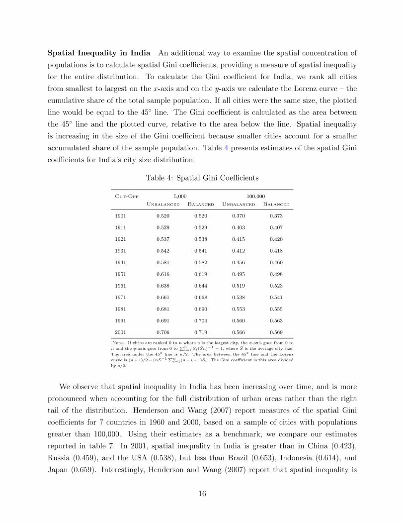
Spatial Inequality in India An additional way to examine the spatial concentration ofpopulations is to calculate spatial Gini coefficients, providing a measure of spatial inequalityfor the entire distribution. To calculate the Gini coefficient for India, we rank all citiesfrom smallest to largest on the x-axis and on the y-axis we calculate the Lorenz curve – thecumulative share of the total sample population. If all cities were the same size, the plottedline would be equal to the 45◦ line. The Gini coefficient is calculated as the area betweenthe 45◦ line and the plotted curve, relative to the area below the line. Spatial inequalityis increasing in the size of the Gini coefficient because smaller cities account for a smalleraccumulated share of the sample population. Table 4 presents estimates of the spatial Ginicoefficients for India’s city size distribution.

Table 4: Spatial Gini Coefficients

Cut-Off 5,000 100,000Unbalanced Balanced Unbalanced Balanced

1901 0.520 0.520 0.370 0.373

1911 0.529 0.529 0.403 0.407

1921 0.537 0.538 0.415 0.420

1931 0.542 0.541 0.412 0.418

1941 0.581 0.582 0.456 0.460

1951 0.616 0.619 0.495 0.498

1961 0.638 0.644 0.519 0.523

1971 0.661 0.668 0.538 0.541

1981 0.681 0.690 0.553 0.555

1991 0.691 0.704 0.560 0.563

2001 0.706 0.719 0.566 0.569

Notes: If cities are ranked 0 to n where n is the largest city, the x-axis goes from 0 ton and the y-axis goes from 0 to

∑ni=1 Si(S̄n)−1 = 1, where S̄ is the average city size.

The area under the 45◦ line is n/2. The area between the 45◦ line and the Lorenzcurve is (n+ 1)/2− (nS̄−1 ∑n

i=1(n− i+ 1)Si. The Gini coefficient is this area dividedby s/2.

We observe that spatial inequality in India has been increasing over time, and is morepronounced when accounting for the full distribution of urban areas rather than the righttail of the distribution. Henderson and Wang (2007) report measures of the spatial Ginicoefficients for 7 countries in 1960 and 2000, based on a sample of cities with populationsgreater than 100,000. Using their estimates as a benchmark, we compare our estimatesreported in table 7. In 2001, spatial inequality in India is greater than in China (0.423),Russia (0.459), and the USA (0.538), but less than Brazil (0.653), Indonesia (0.614), andJapan (0.659). Interestingly, Henderson and Wang (2007) report that spatial inequality is

16

declining over time globally, and in both developed and developing countries. However,spatial inequality has increased over this time in India.

Zipf’s Law and Primate Cities in India The stability of the city size distributionsacross countries and over time have led some to argue that they are either globally (Gabaix,1999) or locally (Eeckhout, 2004; Duranton, 2007) approximated by a Pareto distributionand thus obey Zipf’s law (Zipf, 1949). Zipf’s law states that the number of cities of sizegreater than S is proportional to 1/S. More formally, city sizes are said to satisfy Zipf’s lawif, for large sizes S, we have,

P (Size > S) =α

Sζ

where α is a positive constant and ζ = 1. This relationship has been explored and shownto hold consistently – and persistently – in many countries and over long periods of time(Rosen and Resnick, 1980; Gabaix, 1999; Soo, 2005; Dobkins and Ioannides, 2000; Black andHenderson, 2003; Ioannides and Overman, 2003; Gabaix and Ioannides, 2004; Rozenfeld etal., 2011).

Following the approach in Gabaix and Ibragimov (2011), I estimate the bias-correctedZipf regression, fitting an ordinary least squares (OLS) regression of the log rank i on thelog size S(i) for each decade,

log(ni − 1/2) = α− ζn logSi

For a sufficiently large n, the coefficient ζn tends with probability 1 to the true ζ. Underthe assumption that Zipf’s law holds, ζn should tend towards 1. Following Gabaix and Ibrag-imov (2011), asymptotically standard errors are estimated following the equation, (2/n)1/2ζ,because OLS standard errors considerably underestimate the true standard deviation of theOLS coefficient ζn. Consequently, taking the OLS estimates of standard errors at face valuewill lead one to reject the true numerical value of ζn too often.5 Before evaluating the em-pirical evidence, it is important to keep in mind the following, discussed by Gabaix andIoannides (2004). They argue that the focus of empirical work on Zipf’s law should be onhow well the theory fits, rather than whether or not it fits perfectly, i.e., the debate of Zipf’slaw should be cast in terms of how well, or poorly, it fits, rather than whether it can berejected or not.

Table 5 presents the results of this exercise for various cut-offs in city size.Columns 1 and 2 present estimates of ζn at the national level. We observe that the

5Results are robust to the standard OLS procedure discussed in Gabaix and Ionnides (2004).

17

Table 5: Statistics on the OLS coefficient ζn

All India All India Within Zone Within Zone

(1) (2) (3) (4)Cut-Off 5,000 100,000 5,000 100,000

ζn # cities ζn # cities ζZn # cities ζZn # cities

1901 -1.350 1,208 -1.541 24 -1.316 1,208 -1.137 24(0.055) (0.444) (0.053) (0.328)

1911 -1.340 1,180 -1.410 23 -1.293 1,180 -1.070 23(0.055) (0.415) (0.053) (0.315)

1921 -1.324 1,237 -1.435 28 -1.289 1,236 -1.136 28(0.053) (0.383) (0.051) (0.303)

1931 -1.295 1,400 -1.445 31 -1.272 1,400 -1.220 31(0.049) (0.367) (0.048) (0.309)

1941 -1.223 1,604 -1.404 47 -1.214 1,604 -1.203 47(0.043) (0.289) (0.042) (0.248)

1951 -1.143 1,847 -1.326 69 -1.138 1,847 -1.199 69(0.038) (0.225) (0.037) (0.204)

1961 -1.095 2,066 -1.284 103 -1.049 2,066 -1.108 103(0.034) (0.178) (0.032) (0.154)

1971 -1.044 2,415 -1.249 149 -0.995 2,413 -1.152 149(0.030) (0.144) (0.029) (0.133)

1981 -1.004 3,117 -1.218 220 -0.989 3,117 -1.113 220(0.025) (0.116) (0.025) (0.106)

1991 -0.979 3,787 -1.206 319 -0.961 3,787 -1.119 319(0.022) (0.095) (0.022) (0.088)

2001 -0.957 4,929 -1.203 441 -0.934 4,929 -1.138 441(0.019) (0.081) (0.018) (0.076)

Notes: Asymptotic standard errors are estimated following Gabaix and Ibragimov (2011).

coefficient on ζn is substantially larger than 1 for most cut-offs. These values are substantiallylarger than the values recorded in the US. For example, in the United States, Gabaix (1999)shows that the ζn coefficient is 1.005 for the 135 largest Metropolitan areas. By contrast, thecoefficient in India for the 135 largest urban areas is 1.29 in 2001 and 1.49 in 1901. From theresults in table 5, we see that the coefficient estimates decrease in size over time, presumablydriven, at least in part, by an increase in the sample size. However, when looking at theright tail of the city size distribution, we observe that none of the coefficient estimates fallwithin even generous bounds – as reported in Gabaix and Ionnides (2004), [0.8, 1.2] – of trueζ.

Surprisingly, zip’s law can better explain the data when accounting for all urban areas,i.e., towns and cities with over 5,000 people. However, even when an upper bound of 1.2 is

18

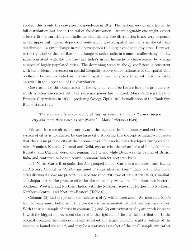
applied, this is only the case after independence in 1947. The performance of zip’s law in thefull distribution but not in the tail of the distribution – where arguably one might expecta better fit – is surprising and indicates that the city size distribution is not very dispersedin the upper tail. Lower slope coefficients imply greater spatial inequality in the city sizedistribution – a given change in rank corresponds to a larger change in city sizes. However,in the right tail of the distribution, a change in rank results in a much smaller change in citysizes, consistent with the premise that India’s urban hierarchy is characterised by a largenumber of highly populated cities. The decreasing trend in the ζn coefficient is consistentwith the evidence presented on spatial inequality above where estimates of the spatial Ginicoefficient by year indicated an increase in spatial inequality over time, with less inequalityobserved in the upper tail of the distribution.

One reason for this compression in the right tail could be India’s lack of a primate city,which is often associated with the rank-size power law. Indeed, Mark Jefferson’s Law ofPrimate City written in 1939 – predating George Zipf’s 1949 formalisation of the Rank SizeRule – states that,

“The primate city is commonly at least as twice as large as the next largestcity and more than twice as significant.” – Mark Jefferson (1939)

Primate cities are often, but not always, the capital cities in a country and exist when asystem of cities is dominated by one large city. Applying this concept to India, we observethat there is no primate city at the national level. Four nodal cities developed during colonialrule - Mumbai, Kolkata, Chennai and Delhi, characterise the urban hubs of India. Mumbai,Kolkata, and Chennai were, and remain, port cities, while Delhi was the capital of BritishIndia and continues to be the central economic hub for northern India.

In 1956 the States Reorganisation Act grouped Indian States into six zones, each havingan Advisory Council to “develop the habit of cooperative working.” Each of the four nodalcities discussed above are present in a separate zone, with two other historic cities, Guwahatiand Jaipur, set as the primate cities for the remaining two zones. The zones are Eastern,Southern, Western, and Northern India, with the Northern zone split further into Northern,Northern-Central, and Northern-Eastern (Table 6).

Columns (3) and (4) present the estimates of ζn within each zone. We note that Zipf’slaw performs much better in fitting the data when estimated within these historical zones.With the same sample of cities in columns (1) and (2) our estimates of ζn are much closer to1, with the biggest improvement observed in the right tail of the city size distribution. In thecolonial decades, the coefficient is still substantially larger but only slightly outside of themaximum bound set at 1.2, and may be a statistical artefact of the small sample size rather

19

Table 6: The Zones of India

Northern Northern-Central Northern-Eastern

Haryana Bihar Assam

Himachal Pradesh Madhya Pradesh Arunachal Pradesh

Jammu & Kashmir Uttar Pradesh Manipur

Punjab Uttaranchal Meghalaya

Rajasthan Delhi Mizoram

Chandigarh Nagaland

Tripura

Eastern Southern Western

Chhatisgarh Goa Andhra Pradesh

Jharkhand Gujara Karnataka

Orissa Maharashtra Kerala

Sikkim Dadra & Nagar Haveli Tamil Nadu

West Bengal Daman & Diu Lakshadweep

Andaman & Nicobar Islands Pondicherry

than anything fundamentally associated with the urban hierarchy in colonial times. Thatbeing said, the coefficient converges to 1 very quickly in the decades following independencefor the full city size distribution and falls well within the maximum bound for the upper tailof the distribution. In addition, the coefficient remains very stable in the decades followingindependence.

Gibrat’s Law and Big(ger) City Bias Given the instability of Zipf’s law at the nationallevel, it is interesting to explore the validity of Gibrat’s law (from which Zipf’s law emerges)which states that city growth rates are orthogonal to city size. We estimate a simple modelof city size growth,

∆ln(Sit) = βlnSit−1 + αi + αt + εit

where we are testing the hypothesis that β = 0. Table 7 presents the results from thisanalysis.

20

Table 7: An Empirical test of Gibrat’s Law

(1) (2) (3) (4) (5) (6)

Cut-Off 5,000 100,000 5,000 100,000 5,000 100,000

logS(i) 0.051*** 0.016 0.113*** 0.0264 0.232*** 0.401***(0.002) (0.009) (0.004) (0.025) (0.018) (0.132)

Year Fixed Effects Yes Yes No No Yes Yes

City Fixed Effects No No Yes Yes Yes Yes

Observations 19,284 1,403 19,284 1,403 19,284 1,403# Cities 3,806 435 3,806 435 3,806 435Adjusted R2 0.197 0.032 0.277 0.405 0.384 0.542

Notes: Robust standard errors are clustered at the city level.

The data rejects Gibrat’s law when looking at the entire distribution of urban locations,consistent with the evidence presented in Holmes and Lee (2010). We are unable to rejectthe null hypothesis in columns (2) and (4) when focussing upon the right tail of the citysize distribution, consistent with Eeckhout (2004); however, once we control for both cityfixed effects and a country-level time trend, we reject the null hypothesis for both the entiredistribution and the right tail of the city size distribution. These results are interesting inso far as they imply that, on average, larger cities grow faster than smaller cities in theurbanisation process. This result is in direct contrast to the results presented in Hendersonand Wang (2007), who estimate significant negative coefficients consistent with a theory ofmean reversion, using the same model for 2,684 cities with more than 100,000 people in 137countries, between 1960 and 2000. However, it is consistent with Michaels et al. (2012) andDesmet and Rappaport (2013), who find positive growth effects for medium-sized locations,relating their observations to either the declining share of land in production as agriculturalareas transition into industry, or to increasing agglomeration economies arising from theintroduction of new technologies.

Why might larger cities grow more quickly than smaller cities? As discussed above,larger cities might grow faster than smaller cities if the ratio of scale economies to scalediseconomies is increasing at a faster rate in larger cities than in smaller cities. This mayoccur if scale economies are increasing relative to diseconomies, or if scale diseconomies havedissipated with technological progress. The speed at which cities grow is likely to dependon their stage in the development process. Henderson and Venables (2009) present a theoryof dynamic city formation in which cities form and grow sequentially, with the largest citiesbeing the first to grow until they reach a critical size, resulting in the next city growing, andso continues the sequence. Cuberes (2011) provides an empirical analysis of the evolution of

21

city growth between 1800–2000, asking which part of the city size distribution the fastest-growing cities fall in each decade. We replicate this analysis for India, asking, for a givendecade, whether large or small cities grow the fastest, and whether this pattern changes overtime.

We begin by ranking each city in terms of population for each decade, with the largestcity ranked 1st. Next, we calculate the 75th percentile of cities’ growth rates and restrictthe sample of cities to those whose growth rate is greater than or equal to this threshold.Finally, we calculate the average rank for those cities to answer whether larger or smallercities grow faster and whether, on average, this pattern changes over time. Earlier in thedevelopment process we should expect that larger cities grow faster, due to the benefits ofeconomies of scale; however, as these cities grow larger, diseconomies of scale become moreimportant for these larger cities, creating an advantage for smaller cities.

Figure 9 presents the results of this exercise for both the entire distribution of cities, aswell as the right tail of the distribution between 1901 and 2001. We observe that in theearly stages of urbanisation, larger Indian cities grow the fastest (the average rank is 585for the entire distribution and 10 for the right tail of the distribution); however, eventuallythe medium and small cities are the ones that attract greater growth, as the average rankincreases.

Figure 9: The Evolution of the Average Rank of the Fastest-Growing Cities in India

However, a concern with this approach is that the average rank will increase over timemechanically, distorting our interpretation of the facts. As the number of cities increases,the interpretation of the rank changes, e.g., an average rank of 10 has a completely differentinterpretation when there are 20 cities, compared to when there are 2,000 cities. Conse-quently, we normalise the average rank by dividing by the number of cities. This providesan interpretation of the average rank in terms of city size percentiles. Figure 10 presents the

22

outcome of this adjustment.

Figure 10: The Evolution of the Average Rank of the Fastest-Growing Cities in India

By adjusting the average rank to account for the number of cities we observe an entirelydifferent picture to the empirical support for sequential growth presented by Cuberes (2011).When looking at the entire distribution of cities, we observe that while there is an increasingtrend over time, the dispersion is very limited, with all adjustment within 10 percentagepoints of the city size distribution, and a difference of 6 percentage points between 1911and 2001. Moreover, the average rank in terms of city size percentiles across this period isthe 54th percentile, far removed from the largest or smallest cities. When we restrict ourattention to cities with 100,000 people or more – the right tail of the city size distribution – wesee a substantially different pattern. There appears to be a cyclicality of growth, with higherranked cities growing faster, followed by lower ranked cities, and so on. In the beginning ofthis time period, this dispersion in average rank is greater than that observed in the entiredistribution, ranging 20 percentage points between the 40th and 60th percentile; however, asurbanisation progresses, this dispersion falls such that between during the last cycle 1971–2001 the range is 5 percentage points. In fact, the dispersion appears to have a half-lifeof 30–40 years. As with the entire city size distribution, the average rank in terms of citysize percentiles between 1911 and 2001 is around the median of the city size distribution,the 48th percentile – far removed from the smallest or largest cities. This is consistentwith the findings of Michaels, Redding and Rauch (2012), who in analyzing populationdensity and growth in the US between 1880–2000 observe a U-shaped relationship thatbecomes flat for high-density locations. They estimate that low-density locations exhibit anegative relationship between 1880 density and growth over the 1880–2000 period, and thathigh-density locations have an orthogonal relationship between 1880 density and populationgrowth. It is in the medium-density locations that the relationship between initial density

23

and growth is positive, consistent with our findings. Michaels et al. (2012) relate this findingto structural transformation, arguing that divergent growth is most prominent in areas thatare transitioning from agriculture into manufacturing. By contrast, Desmet and Rappaport(2013), who observe a similar pattern of positive growth in medium-sized US locations, arguein favour of an explanation associated with increasing agglomoration economies due to theintroduction of new technologies, as in Desmet and Rossi-Hansberg (2009).

The historical record of urbanisation in India, as portrayed by the data presented here,suggests slow yet steady progress over the last century; however, there is increasing evidencethat the pace of urbanisation has been increasing more recently, driven by India’s changingdemographic and geographic landscape. The following sections explore how recent urban-isation has tied into the spatial distribution of economic activity, alongside a discussion ofthe evidence on population mobility and migration, and investments in urban amenities andinfrastructure.

Too Big, Too Small, Or Just Right? The evidence presented in this section indicatesthat, while slow, urbanisation is starting to take off in India. This process of urbanisationhas been characterised by: substantial growth in the size of large cities (the right tail of thecity size distribution), resulting in an increase in spatial inequality over time; substantialgrowth in the number of large cities, resulting in the absence of a national primate cityand the rejection of Zipf’s law at the national level; and the expansion of large cities intosuburban and peri-urban areas. Furthermore, we observe that cities in the middle of thedistribution are growing faster than larger or smaller cities, which indicates an increase inthe number of large cities in the future.A number of questions remain. First, what are the drivers, and consequences, of these factorsin shaping the spatial allocation of resources, people, and economic activity? Is a focus onlarger cities efficient? What are the welfare consequences of having an urban system that isskewed towards larger cities? Should policy makers focus resources on encouraging smallercities to grow, or invest in infrastructure to allow larger cities to better support urbanisation?Future research should aim to better understand these questions; however, the absence ofcity-level data in India creates a number of difficulties. Unlike China, Brazil, and the UnitedStates, India does not collect data systematically at the city level. Without data on economicoutput, prices and wages it is very difficult to understand the economic consequences ofurbanisation in India. Furthermore, economic activity is mainly identified at the districtlevel, limiting the degree to which we can understand the spatial distribution of industryand its relationship to urbanisation.

24

One source of data that may provide an avenue for future research on urbanisation in Indiais the economic census, collected every 8-10 years (1977, 1980, 1990, 1998, 2005, 2013). Theeconomic census is a complete enumeration of all establishments except those engaged in cropproduction and plantation; there is no minimum firm size, and both formal and informalestablishments are included. However, the most interesting characteristic of the data is thedetail provided on spatial location and industrial sector, available at the village level for ruralareas and ward-block level for urban areas – subdivisions of a town or city (see Asher andNovosad (2013) for more detail). The combination of this data with data on price indices andwages at the district level from the National Sample Survey (hereafter, NSS) would providea rich dataset to better understand what determines the spatial allocation of resources,people and economic activity, and the impacts of urbanisation on growth and development.Combined with data on night lights, alternative measures of urban classification can bedeveloped to explore the effects of urbanisation within and between rural and urban areas.

4 Urbanisation and the Spatial Distribution of Economic

Activity

While India’s urban development has followed a gradual yet unabated rise since indepen-dence, economic development has taken much longer to get started. Post independence in1947, India set out on a period of centrally planned industrialisation. The theoretical argu-ment was that massive state investment would help kick-start development and that statecoordination of economic activities would ensure the rapid and sustained growth of domesticindustries (Rosenstein-Rodan, 1943; 1961; Rostow, 1952).

The focal point of the planning regime was the Industries Act of 1951, which introduceda system of industrial licensing that regulated and restricted the entry of new firms as well asthe expansion of existing ones. This system of industrial regulation that controlled the paceand pattern of industrial development became commonly known as the “license raj”. Theemphasis on central planning is most clearly demonstrated by the Industries Act of 1951,which states that ‘it is expedient and in the public interest that the Union should take underits control the industries in First Schedule.’ 6

While the intention of such policies was to kick-start development, in practice this periodof central planning stifled innovation and reduced production and investment. It also reducedefficiency, due to the elimination of competition, both internationally and through barriers to

6Union refers to the central government. The First Schedule lists all key manufacturing industries in1951 and is subsequently revised to encompass new products. The central planning act effectively brings allkey industries under central government control via licensing (Malik, 1997).

25

entry for new firms. Furthermore, the bureaucratic nature of the licensing process imposeda substantial administrative burden on firms, with paper work expected every 6 months andadditional applications required for additional changes in production.

In addition, there was considerable uncertainty as to whether license applications wouldeven be approved and, if they were, when the approval would be granted. Hazari (1966)notes that 35% of license applications were rejected in 1959 and 1960, with the rejectedapplications accounting for nearly 50% of the total investment value among the applicantpool. This, of course, does not even take into account the investments that did not reachthe license application stage.

The result of this inward-oriented, centrally planned industrialisation was three decades oflow and stagnant growth (3.5% per year between 1950 and 1980). By contrast, the East Asianeconomies of Hong Kong, Singapore, South Korea, and Taiwan experienced extraordinarilyhigh growth rates of around 10% per year over the same period. The fundamental differencein these economies is that the investments made were productive and that production wasoutward-oriented, resulting in imports of equipment that resulted in technological changeand further productivity increases.

To the degree that the model of urbanisation discussed in the previous section is reason-able – i.e., that the transition from an agrarian society to a modern economy begins withthe movement of workers from the agricultural sector into industrial production and services–, it is unsurprising that the pace of urbanisation during this period could be described asslow compared to other developing countries at similar stages of development.

Recognition of the issues associated with the centrally planned industrialisation strategy– namely, the persistent stagnation of the Indian economy – prompted the government toundertake a set of liberalisation reforms in the 1980s and more forcefully in the early 1990s.In 1980, Indira Gandhi made the 1980 Statement on Industrial Policy, signalling a renewedemphasis on economic growth (Government of India, 1980). However, it was not until RajivGandhi unexpectedly came to power, following his mother’s assassination in 1984, thatlarge-scale reform entered the political agenda. About a third of three-digit industries wereexempted from industrial licensing or de-licensed in 1985 (with few extensions in 1986 and1987). However, on the 21st of May 1991, Rajiv Gandhi was assassinated in the midst of anelection campaign. Narasimha Rao was appointed as his successor, who in turn appointedManmohan Singh as finance minister. Alongside this political turmoil, rising external debt,exacerbated by a spike in oil prices as a result of the Gulf War, led to a macroeconomic crisisfor India, resulting in external support from the International Monetary Fund (IMF) thatwas conditional on the implementation of a structural adjustment program.

This tipping point resulted in the large-scale liberalisation of the Indian economy and the

26

end of the “license raj”. Industrial license was abolished, additional industries were removedfrom the First Schedule, and both tariff and non-tariff barriers were slashed, reducing barriersto trade.

Given the relative increase in urbanisation during the post-liberalisation period, it isof interest to examine the rural-urban differences in industrial production at this time tounderstand the degree to which industrialisation and urbanisation go hand in hand. It iscommon for the biggest cities in developing countries to start off as manufacturing centres.The main economic consideration for such observations is the presence of agglomerationeconomies or increasing returns to scale. Public services, capital markets, the allocationof licenses, knowledge and ideas may all be biased towards these urban centres, creatingattractive environments for production.

However, as development proceeds, industrial production decentralises. This decen-tralisation arises in two stages, first towards peri-urban or suburban areas, then towardsmetropolitan regions, small cities, and rural areas. Henderson (2012) presents this processfor the Republic of Korea and Japan. The World Bank (2013) also examines the case ofKorea, linking decentralisation to the widespread transport and communications infrastruc-ture investments made in the early 1980s. Such investments increase access to agglomerationexternalities associated with urban centres, reducing the need for urban intensification, andconsequently reducing the magnitude of negative externalities such as congestion, crime, andpollution.

This process of decentralisation is also one that is observed in India, although questionsremain as to whether the process of centralisation really began. Two recent studies explorerecent patterns of production in India and how the patterns of production differ between ruraland urban areas. Desmet et al. (forthcoming) study manufacturing employment growth indistricts where manufacturing is already concentrated and in districts where it is not. Theyconduct the same exercise for the services sector. Figure 11 presents the key results fromtheir study.

27

Figure 11: Annual Manufacturing and Services Employment Growth as a function of ini-tial employment density (logs). Manufacturing results based on NSS and ASI, 2000–2005.Services Results based on NSS, 2001–2006

Between 2000 and 2005, districts with higher concentrations of manufacturing employ-ment grow much more slowly than districts with lower concentrations. In fact, on average,high-concentration districts have negative growth rates and actually lose employment. Bycontrast, the services sector shows increasing growth in districts with higher concentrations.This is suggestive of decentralisation in the manufacturing sector, with the services sectorconcentrating even more in high-intensity districts. Ghani et al. (2012) look more specificallyat manufacturing and document its movement away from cities to rural areas, comparingthe formal and informal sectors. The authors argue that the organised sector is becomingmore rural. However, in practice, a lot of this movement may be suburbanisation – the firststage of decentralisation, in which firms move to the outskirts of major cities, with vastlycheaper land and somewhat cheaper labor. They observe that, while the urban share ofemployment in the formal sector declined, the urban share of employment in the informalsector rose. This may indicate that the scale economies are of greater importance for smallerfirms, while larger firms can break off from centralised locations. For example, a firm withmultiple plants can benefit from scale economies if its headquarters are based in urban areaswith additional production plants exploiting cost reductions in suburban areas.

One of the attractive features of the Annual Survey of Industries is that it distinguishesbetween establishments in rural and urban areas. This is a feature that has not been ex-ploited in the exploration of decentralisation in formal sector manufacturing. Arguably, acomparison between formal sector firms and informal sector firms does not provides a suitablecounterfactual; by contrast, a comparison between formal sector firms in rural and urbanareas may provide more insight into the decentralisation of formal sector manufacturing. Wefollow Desmet et al. (forthcoming) and run nonlinear kernel regressions of the form,

28

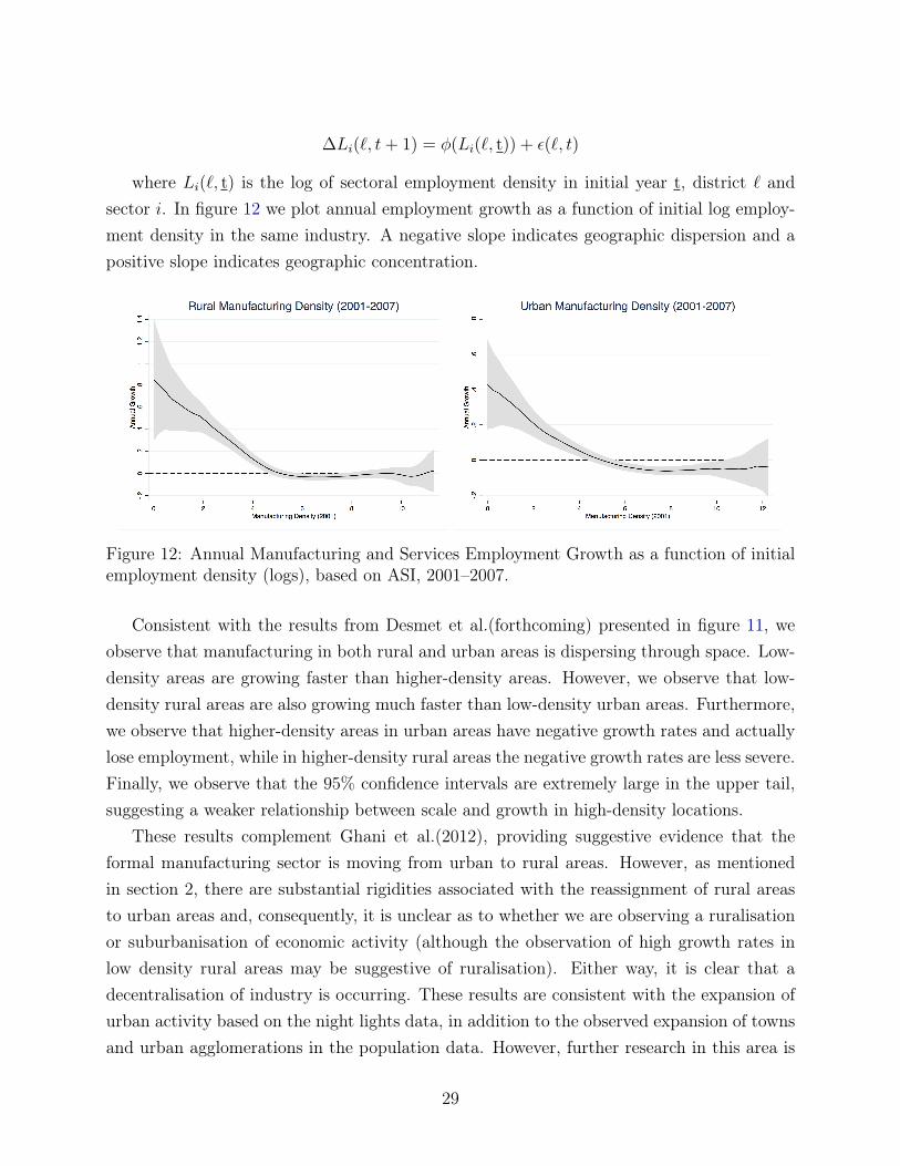
∆Li(`, t+ 1) = φ(Li(`, t)) + ε(`, t)

where Li(`, t) is the log of sectoral employment density in initial year t, district ` andsector i. In figure 12 we plot annual employment growth as a function of initial log employ-ment density in the same industry. A negative slope indicates geographic dispersion and apositive slope indicates geographic concentration.

Figure 12: Annual Manufacturing and Services Employment Growth as a function of initialemployment density (logs), based on ASI, 2001–2007.

Consistent with the results from Desmet et al.(forthcoming) presented in figure 11, weobserve that manufacturing in both rural and urban areas is dispersing through space. Low-density areas are growing faster than higher-density areas. However, we observe that low-density rural areas are also growing much faster than low-density urban areas. Furthermore,we observe that higher-density areas in urban areas have negative growth rates and actuallylose employment, while in higher-density rural areas the negative growth rates are less severe.Finally, we observe that the 95% confidence intervals are extremely large in the upper tail,suggesting a weaker relationship between scale and growth in high-density locations.

These results complement Ghani et al.(2012), providing suggestive evidence that theformal manufacturing sector is moving from urban to rural areas. However, as mentionedin section 2, there are substantial rigidities associated with the reassignment of rural areasto urban areas and, consequently, it is unclear as to whether we are observing a ruralisationor suburbanisation of economic activity (although the observation of high growth rates inlow density rural areas may be suggestive of ruralisation). Either way, it is clear that adecentralisation of industry is occurring. These results are consistent with the expansion ofurban activity based on the night lights data, in addition to the observed expansion of townsand urban agglomerations in the population data. However, further research in this area is

29

needed to understand the consequences of this on welfare and manufacturing productivity.With the decentralisation of industry from urban to rural areas, one might conjecture

whether, as the development process continues, we will see a shift towards consumer cities asdiscussed by Glaeser et al. (2001) and Glaeser and Gottlieb (2006). That is, an exploitationof scale economies by consumers. If so, this may offset concerns that the decentralisationof economic activity in developing countries, particularly in India, is premature. The fol-lowing section explores the returns to urban living, particularly looking at trends in publicinvestments, urban amenities, and poverty in recent times.

5 Urbanisation, Migration, and Amenities

Ultimately, the degree to which scale economies can be exploited depends on the way in whichurbanisation is managed. From an economic efficiency perspective, we want to maximise theproductivity and utility benefits of scale economies; however, policy distortions may offsetthese benefits, reducing scale economies relative to diseconomies. For example, Bertaud andBrueckner (2005) argue that land market regulations limiting floor-area ratios in Mumbaihave exacerbated urban sprawl, resulting in inefficiently low densities near the city centre.Such policies may constrict the social benefits associated with urbanisation. Furthermore, itis of interest from an equity perspective to understand whether the benefits of urbanisationare spread geographically.

To better understand these questions, we explore the degree to which urbanisation hasaffected local standards of living and the provision of public goods and urban amenities.While urbanisation can enhance productivity, it can have deleterious consequences if poorlymanaged. In densely populated areas, the inability to provide local public goods such asclean water and proper sanitation can result in a public health disaster. Limited transportnetworks can increase commuting costs substantially, forcing workers to live in substandardhousing and slums in order to be close to jobs. Finally, we want to understand whether theeconomic gains associated with agglomeration externalities result in poverty reduction andincreased standards of living. An important issue is whether spatial misallocation results inan increase in spatial income inequality.

30

The Network Structure of Cities A major limitation of previous work in this literaturehas been the focus on individual cities as case studies. An important consideration is thegeneral equilibrium nature of urbanisation, which has largely been missed in the empirical lit-erature, despite the theoretical focus on cities as systems. Investments or policy interventionsto attenuate scale diseconomies or amplify scale economies in one location may attract firms,workers and consumers from other location. Similarly, the economic consequences of nega-tive shocks in one location may be mitigated if agents are able to move away (Notowidigdo,2013; Colmer, 2015). In considering the policies that may affect the spatial allocation ofresources, the wider system needs to be taken into account, i.e., one must understand howchanges to one region will affect other regions within the system. Whether discussing the sizeor geometry of cities, or the spatial allocation of economic activity, more evidence is neededto understand the welfare consequences of urbanisation and its implications for growth anddevelopment.Future work aims to examine the degree to which localised productivity shocks or policy in-terventions propagate through the “system of cities” in order to explore how the spatial struc-ture of the economy affects aggregate, rather than local, welfare, growth, and productivity.By explicitly estimating the network structure of cities through, for example, transportationinfrastructure, migration flows, inter-sectoral linkages, or intra-national trade networks, wecan understand whether shocks to individual cities or locations wash out on aggregate, orwhether idiosyncratic shocks affect other locations as well as amplifying, or attenuating, thelocalised effect.

Migration and Transportation Infrastructure

Migration To begin, we examine the patterns of rural-urban migration in recent years toget a clearer idea of the demand for urban living. Migration is a complex phenomenon, yetit has long been thought to play a central role in the efficient allocation of resources. Asarbitrage opportunities arise, marginal migrants move, encouraging equilibrium. However,our understanding of this process has long been constrained by a lack of reliable micro-leveldata on migration. The data we do have indicates that population mobility in India is low.However, in recent decades, internal migration has been on the rise. In the 2001 census, 98million (9.5% of the population) were reported to have migrated in the last decade, basedon the change in residence concept, an average of 0.9% per year.7 This is an increase of 20%compared to the decadal migration rate reported in the 1991 census (82 million, or 9.7% ofthe population). To provide some context, roughly 10% of the households are reported to

7Unfortunately, data on migration from the 2011 census has not yet been released.

31

migrate internally within the United States every year, highlighting the incredibly low levelsof internal migration observed in India over the course of a decade.

In the 2001 census, 82% migrated within the same state, and 60% migrated within thesame district, highlighting the limited mobility of migrants across space in India. Morerecently, round 64 of the NSS (2007–2008) reported that 2.67% of the sample migrated inthe last year, of which 77% was within-state, and 50.13% was within-district.

Of relevance for the process of urbanisation is the degree to which employment acts asa driver of migration for work. In the 2001 census, 14.7% of migrants reported employmentas the reason for migration; however, this number was driven by men, who reported workas the reason 37.6% of the time. In the NSS, employment is reported as the primary reasonfor migration 80% of the time.

Of more explicit relevance for urbanisation is the share of migration between rural andurban areas. 21.1% of census migrants moved from rural to urban areas between 1991and 2001, the largest category after rural-rural migration, which comprised 54% of totalmigration.

The difficulty with analysing migration patterns is that so much of migration in de-veloping countries is seasonal and therefore very difficult to measure, as the likelihood ofsurveying a seasonal migrant depends on the time of year the survey is conducted. Thisalso highlights one of the difficulties associated with the classification of employment in de-veloping countries. Given the seasonality of work, the composition of employment in theeconomy will vary substantially. Consequently, within-year variation in employment likelyvaries considerably in developing countries, although we have little understanding of thenumbers or consequences of this. Colmer (2015) estimates that year-to-year changes in agri-cultural productivity, driven by weather variation, results in substantial labour reallocationbetween agriculture and the manufacturing sector, highlighting this churn in employmentacross sectors.

Round 64 of the NSS has a special schedule on seasonal migration, in which seasonalmigrants are defined as members of the household that are away from the home for morethan 1 month but less than 6 months at a time. In 2007, 14% of households reportedly sentout a member of the family as a seasonal migrant – more than 5 times than the proportionof households that migrated non-seasonally in the previous year. Of these households, 83%were from rural areas, 60% migrated within State, 23% migrated within District; and 87%migrated for work.

This data, while insightful, only provides a snapshot of migration in India. It says nothingabout the subtleties associated with temporary and repeat migration necessary to understandthe consequences of internal migration. Joshua Blumenstock has made considerable progress

32

along this dimension by applying methods in computational statistics to high-resolutiondigital trace data. Through the use of mobile phones, Blumenstock (2012) collects data onthe phone records of 1.5 million Rwandans over four years. For each phone-based transactionrouted through a mobile phone tower, we know the closest tower to the subscriber at thetime of the transaction, allowing us to approximately infer the location and trajectory of1.5 million phone users over time and space. While there are limits to this approach, suchas when users go long periods of time without using their phone, and the selection biasassociated with using a mobile phone (Blumenstock and Eagle, 2012), the use of ICTs toinfer internal migration has the potential to play a major role in future research on migration.

Why is population mobility so low in India? One hypothesis is that local risk-sharingnetworks restrict mobility (Munshi and Rosenzweig, 2009; Morten, 2013). Munshi andRosenzweig (2009) find evidence that caste-based insurance networks, which have helpedhouseholds smooth consumption for centuries, limits out-migration. Morten (2013) exploresthe joint determination of migration and informal risk sharing to understand the welfareeffects of migration on income and the endogenous structure of insurance. She then exploreshow risk sharing alters the returns to migration. She finds that risk sharing reduces migrationby 60%, migration reduces risk sharing by 23%, and that when contrasting endogenous risksharing with exogenous risk share, the consumption equivalent-gain from migration is 7%lower.

Other factors may include low investments in transportation infrastructure (discussed be-low), uncertainty about the likelihood of gaining employment in destination markets (Bryanet al., 2014), or other direct costs. More work is needed to better understand the adjust-ment costs that migrants face, and the consequent misallocation that arises, and whetherthe decision to not migrate is rational and the result of sorting.

Using the available data, we have shown that population mobility in India is low andmainly restricted within-district (23–60%) or within-state (60%–82%). Furthermore, themajority of migration is between rural areas, with only 21% of migration occurring betweenrural and urban areas. However, as previously discussed, the classification of rural andurban areas makes it difficult to interpret these shares. If the destination areas of rural–ruralmigration are suburban or peri-urban areas where we observe decentralised manufacturing isdecentralising towards this will understate the contribution of migration to the urbanisationprocess. Irrespective of classification, it is clear that population mobility is low. This hasimplications for the general equilibrium considerations of urbanisation, since investments orpolicy interventions implemented to attenuate scale diseconomies or amplify scale economiesin one location may have little impact on attracting firms, workers and consumers from otherlocations. More importantly, the economic consequences of negative shocks in one location

33

are likely to be greater if agents are unable to move away (Notowidigdo, 2013; Colmer, 2015).If labour is inelastic, the economic consequences of negative shocks may be amplified if localwages fall further in response to the oversupply of workers (Jayachandran, 2006).

Transportation Infrastructure As discussed, transportation infrastructure may be oneof the factors that explains the limited population mobility observed in India; however,transportation plays a much broader role in the process of urbanisation. Indeed, the trans-portation of goods and people plays a vital role in the spatial organisation of economicactivity (see Turner and Redding (2015) for a recent review of this literature). Historically,transportation technologies have played a major role in the development process, reshap-ing the economic activity connected to them as they themselves have undergone significantchanges over time.

Donaldson (forthcoming) considers some of the earliest investments in Indian transporta-tion infrastructure, examining the effect of railroads on economic activity in colonial-era In-dia. Exploiting the evolution of India’s railroad network between 1860 and 1930 (see figurefigure:raj), he finds that districts with access to railroads report 17% higher real agriculturalincome than districts without railroads. This is a substantial effect considering that, overthe course of the 1870–1930 study period, real agricultural incomes rose by only around 22%.Consequently, a rail connection was equivalent to more than 40 years of economic growth.

Figure 13: The Evolution of India’s Railroad Network: 1860–1930

More recently, Ghani et al. (forthcoming) estimate the effect of the Golden Quadrilateralproject, which upgraded the quality and width of 5,866km of highways in India, presented infigure 14. They find that the project resulted in a significant increase in economic activity andproductivity in non-nodal districts within 10km of the Golden Quadrilateral, but no effectsbeyond this distance. Khanna (2014) also explores the effects of the Golden Quadrilateral

34

upgrades, examining changes in night-time luminosity around the project. He finds evidencefor a spreading-out of economic development, consistent with our discussion surroundingurban sprawl and decentralisation in India.

Figure 14: The Golden Quadrilateral and North-South East-West Highway Systems

There has been a strong focus on the effects of large-scale highway and railroads projectson urbanisation and economic activity in recent years across many countries (Banerjee etal., 2012; Baum-Snow et al.,2014; Donaldson and Hornbeck, 2013; Duration and Turner,2012; Faber, forthcoming; Garcia-Lopez et al., 2013; Hsu and Zhang, 2012; Storeygard,2012). However, there has been very little work on the effects of smaller scale transportationinvestments, such as those in rural areas where the returns may be greater. Asher andNovosad (2014) are an exception. They examine the effects of the Pradhan Mantri GramSadak Yojana (hereafter, PMGSY) project – a nationwide plan to provide good all-weatherroad connectivity to unnconnected villages in rural India–, finding that the provision of anew paved village approach road produces significantly faster employment growth and acorresponding reduction in unemployment. Understanding the effects of rural connectionson rural–urban migration may help to understand part of the reason behind the low levelsof population mobility if transportation costs are reduced, e.g., all-weather roads don’t washaway during the monsoon. In addition, it would be interesting to examine the spillovereffects of rural road connections on agricultural markets, wages, and prices.

An obvious caveat relates to the interpretation of the results across this literature. Itis difficult to know whether the observed effects are the results of growth, or from the

35

reorganisation of economic activity. As discussed in the box above, by estimating the networkstructure of cities, we can estimate the aggregate welfare effects of local investments, ratherthan simply estimating the localised effects.

Housing: Quality and Constraints

A key consideration in any discussion on urbanisation is the supply of housing. As developingcountries grow and develop and urbanisation increases, will the stock of housing be able tokeep pace, or will it deteriorate, reducing the gains from urban living, and ultimately slowingprogress?

We begin by exploring changes in housing quality in the last decade, a period in whichwe have observed an increase in the pace of urbanisation and migration. A concern might bethat investments in urban infrastructure have been insufficient to maintain living conditions;however, during this period we observe that housing conditions in urban areas improvedsubstantially. We observe a 4.2 percentage point increase in the share of good housing,corresponding to a 3.6 percentage point reduction in the share of liveable housing and a0.6 percentage point reduction in the share of dilapidated housing. By contrast, rural areassaw a 1.1 percentage point increase in the share of good housing, but also a 0.2 percentagepoint increase in the share of dilapidated housing, corresponding to a 1.3 percentage pointreduction in the share of liveable housing. These changes are summarised in table 8.

Table 8: Changes in the Quality of the Rural and Urban Housing Stock (2001-2011)

2001 (%) 2011 (%) Difference % Change

Condition Rural Urban Rural Urban Rural Urban Rural Urban

Good 44.8% 64.2% 45.9% 68.4% 1.1 4.2 2.46% 6.54%

Liveable 48.9% 32.3% 47.6% 28.7% -1.3 -3.6 -2.66% -11.15%

Dilapidated 6.3% 3.5% 6.5% 2.9% 0.2 -0.6 3.17% -17.14%

Total 100% 100% 100% 100% 0 0 – –

While, on the face of it, this seems like good news, this data is unlikely to capture livingstandards when there are constraints in access to housing. Urban planning systems in Indiamake it hard to expand and redevelop urban areas (see World Bank, 2013 for an overviewof India’s urban planning system). Mumbai, for example, has stringent land regulations.Indeed, two key features of the land regulation environment in Mumbai stand out. First, ithas an FSI ratio – the ratio of the gross floor area of a building divided by the area of thatlot – of around 1.0-1.5, increasing the incentive for urban sprawl as developers are unable to

36

make efficient use of the lot space if they want to build several stories. For example, with anFSI ratio of 1:1, this means that the total lot space can be used for a one-story building or50% of the lot space can be used for a two-story building. Such restrictions generate sprawlas development is forced to the periphery, consistent with the expansion of urban night lightsin figures 3 and 4.

Such stringent land regulations reduce the housing supply and make it less affordable.In light of this, housing shortages may be a more appropriate measure of living standards.The World Bank (2013) reports that housing shortages in urban India shot up from 3.0million units in 1971 to 24.7 million in 2007, and that urban areas require an additional 1.8million units annually to accommodate new households. The Report of the Working Groupfor the 11th Five-Year plan estimated that there were 66.3 million urban households andan urban housing stock of 58.83 million, a shortage of 7.47 million units. Furthermore, theworking group found that more than 19% of urban households lived in congested conditionsand estimated that 4.6 million units (8%) were either obsolescent or needed to be upgradedfrom a dilapidated to a liveable condition. While there has been considerable progress inestimating the welfare effects of land use regulation in developed economies (Turner et al.,2014) more work is needed to evaluate the welfare consequences in developing economies.

This is indicative that the housing market in India is not keeping pace with the formationof urban households. This will result in inflated housing costs, which will ultimately harmlow-income groups the most, where housing costs form a larger share of total expenses. Thedevelopment of informal settlements – slums – has been a natural consequence of the limitedhousing stock.

Slums Between 2001 and 2011, the population census of India reported an increase in theslum population from 52.371 million people to 65.494 million people, an increase of 13.123million. However, the slum population’s share of urban population decreased over this periodfrom 18.3% to 17.4%. Measurement error is a major concern here as the number of townsreporting slums increased by 870. This is likely to have been driven by a reduction in thenumber of states and union territories not reporting slums. This may explain why othersources report a reduction in India’s slum population. Marx, Stoker and Suri (2013) reporta 10% reduction in the slum population between 1990 and 2007. While these periods arenot comparable, it is important to note that using the same data between 1990 and 2001 weobserve a 20% increase in the slum population, implying that between 2001 and 2007 therewas a 25% reduction in the slum population to result in a slum population that was 10%below 1990 levels.

Some economists (Frankenhoff, 1967; Turner, 1969; Glaeser, 2011) have suggested that

37

slums are a transitory phenomenon in fast-growing economies that will progressively evolveinto formal housing as societies approach the later stages of development. Marx, Stoker andSuri (2013) argue that, even if slum populations are stable in the short or medium run, thisargument still holds, as slum living only represents a transitory phase in the life cycle of ruralmigrants – slum dwellers or their children eventually move into formal housing within thecity. In this respect, slum populations may remain constant but with substantial turnoverin the households that reside in these areas. Indeed, rural–urban migration is prominentin India, so urban productivity must be rising relative to rural productivity, due to eithercapital accumulation and technological progress (Asher and Novosad, 2012; Bustos et al.,2014;Marden, 2014) or declines in rural productivity (Colmer, 2015; Henderson et al. 2014).Furthermore, Bryan et al. (2014) show that seasonal urban migration in Bangladesh cangenerate welfare improvements for families of migrants. Ultimately, it could be argued, basedon revealed preference, that urban poverty is preferable to rural poverty (Glaeser, 2011).

However, this says nothing about the nature of poverty in slums and whether it can beescaped. An expanding literature explores the degree to which slums may arise as the resultof government policy. Cai (2006) explores the provision of local services for urban villages inChina, finding that these “slums” do not receive central water or sewerage services, nor thecollection of rubbish from the city. Furthermore, children living in these areas are excludedfrom state schools. This raises the cost and lowers the quality of access to such services forrural–urban migrants living in slums, increasing the cost of migration to urban areas. Felerand Henderson (2011) estimate the effects of service denial on the population growth forlow-skilled workers in Brazil. In the 1980s, Brazilian localities were not required to serviceareas that were not part of the formal sector. The results of this analysis indicate that insome contexts the emergence of slum populations may reflect, at least in part, the strategicdecisions of local governments to restrict in-migration, especially in favoured cities.

Empirical research in this area is limited due to data collection constraints, such assafety issues and difficulties in the ability to track respondents over time – if the members oftargeted households can be found in the first place. However, there have been a number ofmore recent studies exploring economic behaviour in, and the characteristics of, Indian slums(Banerjee et al., 2011; Banerjee, Duflo, Glennerster and Kinnan, 2014; Marx, Stoker andSuri, 2013). Understanding the welfare consequences of slums is a topic that warrants greaterattention. Indeed, the greatest returns are likely to arise from the systematic collection ofdata – the most binding constraint to research in this area. In addition, the development ofmethods to track individuals and households as they enter and exit slums will provide muchinsight into the micro-dynamics of urbanisation and the welfare consequences thereof.

38

Measuring Mobility with Mobiles A question of economic and policy importance is thedegree to which slum living represents a transitory phase in the life cycle of its dwellers.However, given data constraints, it is impossible to explore whether this claim is true orwhether slum living is persistent. One opportunity for future research that is of particularinterest builds on the recent work by Blumenstock (2012) and Blumenstock et al. (2014),who exploit large-scale digital trace data to study the mobility and migration patterns ofindividuals in developing countries. As access to mobile technologies increase in developingcountries, and methods in computational statistics further develop, opportunities to trackand explore the mobility patterns of slum dwellers at a higher geographic resolution willbecome available. Access to such data will help us to understand more about the nature ofpoverty in slums and whether it can be escaped.

Amenities and Public Services

Another factor under consideration is the difference in access to public services and basicamenities between rural and urban areas. Greater access to public goods and basic ameni-ties may well be sufficient to offset the adverse conditions in urban areas associated withcongestion. Scale economies increase the social benefit of public investment, especially thosewith network characteristics such as access to electricity.

Table 9: Access to Public Goods and Basic Amenities in Rural and Urban Areas(1991-2011)

Improved Sanitation Improved Water Source Access to Electricity

Rural Urban Rural Urban Rural Urban

1991 6.6% 50.1% 65.2% 89.1% – –

2001 15.3% 54.9% 77.3% 92.7% 45.53% 87.58%

2011 23.9% 59.7% 89.5% 96.3 % 55.30% 92.70%

Energy In table 9 we observe that there has been a steady increase in access to electricityin both rural and urban areas between 2001 and 2011; however, there is a stark differencein access between the two. Access to electricity in urban areas is almost complete, whereasin rural areas only 55% of households have access to electricity. On the other hand, beingconnected to the grid tells us very little about the quality of access to electricity. On the30th of July 2012, India’s electricity grid faltered, meaning that an area with more than halfof the country’s population went dark – the largest power failure in history. However, in

39

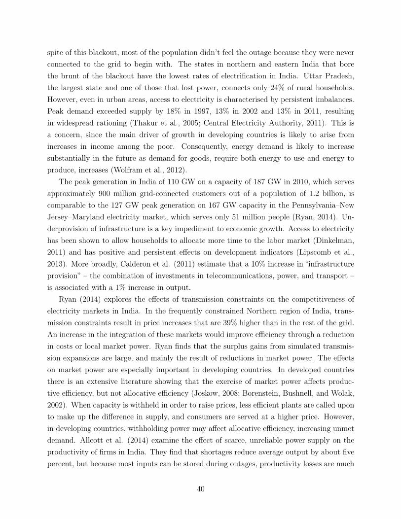
spite of this blackout, most of the population didn’t feel the outage because they were neverconnected to the grid to begin with. The states in northern and eastern India that borethe brunt of the blackout have the lowest rates of electrification in India. Uttar Pradesh,the largest state and one of those that lost power, connects only 24% of rural households.However, even in urban areas, access to electricity is characterised by persistent imbalances.Peak demand exceeded supply by 18% in 1997, 13% in 2002 and 13% in 2011, resultingin widespread rationing (Thakur et al., 2005; Central Electricity Authority, 2011). This isa concern, since the main driver of growth in developing countries is likely to arise fromincreases in income among the poor. Consequently, energy demand is likely to increasesubstantially in the future as demand for goods, require both energy to use and energy toproduce, increases (Wolfram et al., 2012).

The peak generation in India of 110 GW on a capacity of 187 GW in 2010, which servesapproximately 900 million grid-connected customers out of a population of 1.2 billion, iscomparable to the 127 GW peak generation on 167 GW capacity in the Pennsylvania–NewJersey–Maryland electricity market, which serves only 51 million people (Ryan, 2014). Un-derprovision of infrastructure is a key impediment to economic growth. Access to electricityhas been shown to allow households to allocate more time to the labor market (Dinkelman,2011) and has positive and persistent effects on development indicators (Lipscomb et al.,2013). More broadly, Calderon et al. (2011) estimate that a 10% increase in “infrastructureprovision” – the combination of investments in telecommunications, power, and transport –is associated with a 1% increase in output.

Ryan (2014) explores the effects of transmission constraints on the competitiveness ofelectricity markets in India. In the frequently constrained Northern region of India, trans-mission constraints result in price increases that are 39% higher than in the rest of the grid.An increase in the integration of these markets would improve efficiency through a reductionin costs or local market power. Ryan finds that the surplus gains from simulated transmis-sion expansions are large, and mainly the result of reductions in market power. The effectson market power are especially important in developing countries. In developed countriesthere is an extensive literature showing that the exercise of market power affects produc-tive efficiency, but not allocative efficiency (Joskow, 2008; Borenstein, Bushnell, and Wolak,2002). When capacity is withheld in order to raise prices, less efficient plants are called uponto make up the difference in supply, and consumers are served at a higher price. However,in developing countries, withholding power may affect allocative efficiency, increasing unmetdemand. Allcott et al. (2014) examine the effect of scarce, unreliable power supply on theproductivity of firms in India. They find that shortages reduce average output by about fivepercent, but because most inputs can be stored during outages, productivity losses are much

40

smaller. Consistent with the hypothesis of unmet demand, plants without generators havemuch larger losses; however, because of economies of scale in generator capacity, shortagesare more costly to small plants. Together, these papers highlight the welfare costs of poorenergy infrastructure in India.

Sanitation and Health Other public goods relate to health capital. A wide literature hasdocumented the importance of health for income and of early-life investments in health forlater-life outcomes (see Lopez-Casasnovas et al. 2005; Bleakley, 2010; and Currie and Vogl,2013 for good reviews of the literature). There are large returns to health improvementsas well as strong complementarities between child health and child education (Miguel andKremer, 2004). As a consequence, differences in human capital and limited infrastructureavailable to make investments may lead to reduced social mobility across generations. Accessto improved sanitation and improved water sources are associated with combating a broadrange of public health issues, such as exposure to bacterial agents and contaminated drinkingwater. Drawing on data from the world development indicators, we observe that there havebeen improving trends in both rural and urban areas over time. The greatest progress hasbeen seen in access to improved water sources. Since 1991, access in rural areas has increasedby around 25 percentage points from 65% to nearly 90%. Urban areas have shown modestimprovements as well, but have started from an already high level, improving from 90% in1991 to 96% in 2011. A major concern in both rural and urban India relates to access toimproved sanitation infrastructure. Access is very low in rural areas, reaching only 24% ofthe population in 2011. However, even in urban areas, only 60% of the urban populationhas access to improved sanitation infrastructure. While this is a substantial improvementon rural outcomes, it is still low by international standards.

Based on data from the 2005–2006 National Family Health Survey, the percentage of slumhouseholds with access to private latrines, open defecation and private water sources paint asimilar urban picture, outperforming rural areas. 75% of households have access to a privatewater source, 32% have access to a private latrine, and 51% engage in open defecation or usea pit toilet. While the measures are not comparable with the WDI indicators, a consistentpattern emerges, namely that access to improved water sources is much more prevalent thanaccess to improved sanitation infrastructure. However, even based on the more restrictivedefinition of improved sanitation in the slum population, sanitation investments are superiorto rural sanitation.

Historically, open defecation has been a major public health issue in India and little haschanged since Mahatma Gandhi famously asserted in 1925, ‘Sanitation is more importantthan independence.’ This is an issue especially for urban areas, since the health externalities

41

associated with public defecation are disastrous when practiced by groups in close contactwith each other. There are also public safety concerns, highlighted by a recent story in May2014, when two teenage girls were raped and murdered after leaving their homes after darkto relieve themselves. Similar attacks are distressingly common. However, there are concernsthat reducing open defecation cannot simply be solved by the construction of toilets. It iswidely believed that open defecation in India is in part the result of cultural practices. Hindutradition, seen in the “Laws of Manu”, encourages open defecation to avoid ritual impurity.Caste structures are another factor, since only the lowliest in society are expected to clearhuman waste.

Pollution and Environmental Regulation A common concern associated with urban-isation and industrialisation in developing countries is the associated increase in pollutionand environmental degradation. It is estimated that every day 1,000 additional vehicles areadded to an already constrained transportation infrastructure, increasing congestion and airpollution. Water pollution is a major source of pollution as well, driven in part by pressureson the sanitation and energy infrastructure needed to process sewage, as well as the diversionof river water for industry and agriculture and the associated flow of industrial and agricul-tural effluents. The Ganges, the 3rd largest river in the world by discharge (38,129 m3/s),provides a clear example of the water pollution problems that India faces. The Ganges is themost sacred river to Hindus, with thousands of devotees performing ablutions in the rivereach day. Water containing more than 500 faecal coliform bacteria per 100 ml is consideredunsafe for bathing. Upstream, the Ganges contains 60,000 bacteria per 100ml. Downstream,where streams of raw sewage empty into the Ganges – and where daily ablutions are per-formed – this figure rises to 1.5 million. These figures provide a clear indication of thepotential health consequences associated with environmental pollution.

However, in spite of these environmental concerns, India has a relatively extensive set ofenvironmental regulations to improve air and water quality. Environmental policy related toair and water pollution is rooted in the Air Act of 1981 and the Water Act of 1974. Theseacts resulted in the creation of the Central Pollution Control Board (CPCB) and the StatePollution Control Boards (SPCBs).

Greenstone and Hanna (2014) provide a more structured analysis of environmental regu-lation in India, examining the effects of the key environmental regulations on air and waterpollution. They estimate that environmental regulations to address air pollution have beenreasonably successful in reducing ambient concentrations of air pollution, particularly the in-troduction of catalytic convertor policies. However, regulation to address water pollution hashad little effect. Consistent with this evidence, we observe a decreasing trend in particulate

42

Figure 15: Air Pollution Trends In India (1985–2007)

Figure 16: Water Pollution Trends In India (1986–2005)

matter and sulfur dioxide emissions, but very little change in nitrogen dioxide emissions. Inaddition, we see little change in water pollution over the last couple of decades. If anythingwe observe small increases in biochemical oxygen demand, and reductions in dissolved oxy-gen, indicating greater pollution as water-borne pollution hinders the mixing of water withthe surrounding air, and hampers oxygen production from aquatic plant photosynthesis.

A remaining question of interest is whether environmental regulation shapes the patternof urbanisation and industrialisation. Particularly, whether environmental regulation withincities encourages decentralisation.

Poverty In addition to examining impacts on the housing supply and on the provisionof public goods and basic amenities, we also want to understand how urbanisation dur-ing the last few decades may have affected living standard more broadly, namely throughpoverty rates. The effects of urbanisation on poverty are ambiguous. On the one hand,scale economies should reduce poverty through increased access to markets and employmentopportunities, as well as improvements in access to public services. However, if urbanisationis managed poorly, then scale diseconomies could increase poverty, offsetting the benefitsassociated with urban living.

Using data from 1983 from the NSS, Panagariya and Mukim (2013) and Panagariyaand More (2014) provide a comprehensive overview of poverty in India. The focus of thisresearch is to compare poverty rates between social groups and examine how poverty rates

43

have changed since the introduction of the Tendulkar poverty lines in 2004; however, thedata also includes differences in rural and urban poverty trends.

In the early 1970s, the Lakdawala committee defined all-India poverty lines for rural andurban areas based on per-capita total consumption expenditures in 1973-74 market prices.The poverty-line consumption baskets were anchored in per-capita calorie norms of 2400 and2100 in rural and urban areas, and provided for the consumption of basic goods and services.The Lakdawala lines served as the official poverty lines until 2004.

In 2004, the Lakdawala poverty lines were adapted to account for three deficiencies, notedby the Tendulkar committee (Planning Commission, 2009). First, the Lakdawala line bas-kets had remained tied to consumption patterns in 1973-74, while consumption baskets haveshifted substantially since then, even for the poor. Secondly, the consumer price index foragricultural workers understated the true price increase. This meant that, over time, theestimated poverty ratios understated rural poverty. Finally, the assumption that health andeducation would be largely provided by the government no longer holds. Private expendi-tures on these services has risen substantially, even for the poor. These critiques saw thedawn of the newly revised Tendulkar poverty lines. The urban poverty line changed to the25.7 percentile of the national distribution of per capita expenditures. The consumptionbasket associated with the national urban poverty line is the same as the rural poverty lineconsumption basket. This entailed the translation of the new urban poverty line using theappropriate price index to obtain the nationwide rural poverty lines. Using this approach,rural and urban poverty lines became fully aligned. The new rural poverty line yielded a ruralpoverty ratio of 41.8% in 2004 compared with 28.3% under the Lakdawala methodology.

Table 10 presents the rural, urban and combined poverty ratios for each social group inIndia between 1993 and 2011, reported in Panagariya and Mukim (2013) and Panagariya andMore (2014). We observe that, over this time, poverty in both rural and urban areas has fallensubstantially. Most surprisingly, it has fallen for the scheduled tribe and scheduled castegroups, though unsurprisingly by less than for non-scheduled groups. This is a significantbreak with past trends, since it indicates that socially disadvantaged groups have caughtup substantially with the better-off groups. Poverty rates have fallen by noticeably more inurban areas than in rural areas across all social groups, to the degree that urban povertyratios are half that of rural poverty ratios.

This indicates that the increasing trends in urbanisation observed during this periodhave corresponded with increases in living standards across the board, relative to ruralareas. However, it is clear that there is still much to be gained from better management ofurbanisation in India to encourage further growth and maximise the returns to agglomerationexternalities and mitigate costs.

44

Table 10: Tendulkar Poverty Rates in India (1993–2011)

Rural

Social Group 1993–94 2004–05 2009–10 2011–12

Scheduled Tribe 65.9% 62.3% 47.4% 45.3%

Scheduled Caste 62.4% 53.5% 42.3% 31.5%

Non-Scheduled Caste 44.0% 35.1% 28.0% 20.3 %

All Groups 50.3% 41.8% 33.3% 25.4%

Urban

Social Group 1993–94 2004–05 2009–10 2011–12

Scheduled Tribe 41.1% 35.5% 30.4% 24.1%

Scheduled Caste 51.7% 40.6% 34.1% 21.7%

Non-Scheduled Caste 28.2% 22.6% 18.0% 11.8 %

All Groups 31.9% 25.7% 20.9% 13.7%

6 Discussion and Policy Implications

Urbanisation in India has been steadily increasing since independence; however, the rate ofurbanisation has been far slower than other countries at similar stages of development. Mostof the growth in urbanisation has occurred recently in the post-liberalisation period duringthe early 1990’s and the high-growth periods that have followed. In characterising India’surbanisation we observe three stylised facts: first, there has been substantive growth in thenumber of urban areas in a demographic sense, yet the relative city size distribution hasremained relatively stable (at least in the tail of the distribution) consistent with evidenceacross countries (Black and Henderson, 2003; Henderson and Wang, 2007).

Second, India’s urbanisation has been characterised by an unusually large number ofhighly-populated cities, with spatial inequality increasing over time. This is supported bythe violation of Zipf’s law and Gibrat’s law at the national level, which we argue arises fromthe absence of a primate city. This is supported by the observance of Zipf’s law within the6 zones of India, each recognised by its own primate city. Questions remain about whatthis implies for growth and development in India. Should policy makers focus resources onencouraging smaller cities to grow, or should they invest in infrastructure to allow larger citiesto better support urbanisation? Future research must focus on understanding the drivers,and consequences, of city growth in shaping the spatial allocation of resources, people, andeconomic activity.

45

Finally, India’s urbanisation has been characterised in a geographic sense by an increasein urban sprawl, with an expansion of peri-urban areas. This is supported by evidence ofdecentralisation in the manufacturing sector, with higher growth rates in low-density areasof “rural” areas. The implications of decentralisation on welfare are ambiguous. On theone hand decentralisation reduces the magnitude of agglomeration externalities. On theother hand, decentralisation also reduces costs and increases rural–urban migration due toreductions in transport costs. In addition, we do not have a clear understanding about thedegree to which firms can exploit agglomeration externalities. If the headquarters of firmsare based in centralised areas, do the fringe plants benefit? Research to better understandthe intersection between production and urban hierarchies should shed light on this question.

In recent years, urbanisation appears to have improved the standard of living in urbanareas, with improvements in housing quality (non-slum) and significant improvements inaccess to public services. However, there are questions as to whether such improvements arehomogenous across income and social groups, as access and quality reflect different outcomes.That being said, significant reductions in poverty have also been observed in urban areas,even for the most socially disadvantaged groups.

What are the implications for policy? Urbanisation is complex and, given its spatialnature, invites discussion on regional policies. However, we simply do not know enoughabout what is efficient and how costly market inefficiency is compared with the costs ofpolicy mistakes.

In the absence of credible evidence, India, as well as other developing countries, shouldfocus on leveling the playing field. This means that policy should focus on eliminatingspatial biases and, where possible, avoid targeting specific cities with favourable economicconditions. This will allow new cities to form and industries to decline and emerge in away that reflects underlying market forces, and will more likely approximate a reasonablyefficient outcome, relative to an outcome that is the result of “picking winners”.

References

Abrahams, Lozano-Gracia, and Oram (2014): “Correcting Overglow in NighttimeLights Data,” mimeo.

Allcott, H., A. Collard-Wexler, and S. O’Connel (2014): “How do ElectricityShortages Affect Productivity? Evidence from India,” NBER Working Paper No. 19977.

Asher, S. and P. Novosad (2012): “Factory Farming: The Impact of Agricultural Outputon Local Economic Activity in India,” Mimeo.

46

——— (2013): “Politics and Local Economic Growth: Evidence from India,” Mimeo.

——— (2014): “The Employment Effects of Road Construction in Rural India,” Mimeo.

Authority, C. E. (2011): “Growth fo Electricity Sector in India from 1947–2011,” CentralElectricity Authority, Ministry of Power.

Banerjee, A., E. Duflo, R. Glennerster, and C. Kinnan (2014): “The Miracle ofMicrofinance? Evidence from a Randomized Evaluation,” Mimeo.

Banerjee, A., R. Pande, Y. Vaidya, M. Walton, and J. Weaver (2011): “Delhi’sSlum-Dwellers: Deprivation, Preferences and Political Engagement among the UrbanPoor,” IGC Conference Proceedings (Growth Week 2011).

Baum-Snow, N., L. Brandt, J. Henderson, M. Turner, and Q. Zhang (2014):“Roads, Railroads, and Decentralization of Chinese Cities,” Mimeo.

Bertaud, A. (2002): “The Economic Impact of Land and Urban Planning Regulations inIndia,” Mimeo.

——— (2004): “The Spatial Organization of Cities: Deliberate Outcome or UnforeseenConsequence?” Mimeo.

Bertaud, A. and J. Brueckner (2005): “Analyzing Building-Height Restrictions: Pre-dicted Impacts and Welfare Costs,” Regional Science and Urban Economics, 35, 109–125.

Black, D. and J. Henderson (2003): “Urban Evolution in the USA,” Journal of Eco-nomic Geography.

Bleakley, H. (2010): “Health, Human Capital and Development,” Annual Review of Eco-nomics, 2, 283–310.

Blumenstock, J. (2012): “Inferring Patterns of Internal Migration from Mobile PhoneCall Records,” Information Technology for Development, 18, 107–125.

Blumenstock, J., R. Chokkalingham, V. Gaikwad, and S. Kondepudi (2014):“Probablistic Inference of Unknown Locations: Exploiting Collective Behaviour when In-dividual Data is Scarce,” ACM Computing for Development (DEV 2014).

Blumenstock, J. and N. Eagle (2012): “Divided We Call: Disparities in Access and Useof Mobile Phones in Rwanda,” Information Technology and International Development.

47

Borenstein, S., J. Bushnell, and F. Wolak (2002): “Measuring Market Inefficienciesin California’s Restructured Wholesale Electricity Market,” American Economic Review,92, 1376–1405.

Brueckner, J. and K. Sridhar (2012): “Measuring Welfare Gains from Relaxation ofLand-Use Restrictons: The Case of India’s Building-Height Limits,” Regional Science andUrban Economics, 42, 1061–67.

Bryan, G., S. Chowdhury, and A. Mobarak (2014): “Underinvestment in a ProfitableTechnology: The Case of Seasonal Migration in Bangladesh,” Econometrica, 82, 1671–1748.

Bustos, P., B. Caprettini, and J. Ponticelli (2014): “Agricultural Productivity andStructural Transformation: Evidence from Brazil,” Mimeo.

Cai, F. (2006): “Floating Populations: Urbanization with Chinese Characteristics,” Mimeo.

Calderon, C., M.-B. E. and L. Serven (2011): “Is Infrastructur Capital Productive? ADynamic Heterogeneous Approach,” World Bank Policy Research Working Paper 5682.

Colmer, J. (2015): “Agricultural Productivity, Labour Reallocation, and Industrial Pro-duction in the Short Run: Evidence from India,” Mimeo.

Cuberes, D. (2009): “Sequential City Growth: Empirical Evidence,” Journal of UrbanEconomics, 69.

Currie, J. and T. Vogl (2013): “Early-Life Health and Adult Circumstance in DevelopingCountries,” Annual Review of Economics, 5, 1–36.

Desmet, K., E. Ghani, S. O’Connel, and E. Rossi-Hansberg (forthcoming): “TheSpatial Development of India,” Journal of Regional Science.

Desmet, K. and J. Rappaport (2013): “The Settlement of the United States, 1800–200:The Long Transition to Gibrat’s Law,” CEPR Discussion Paper 9353.

Dinkelman, T. (2011): “The Effects of Rural Electrification on Employment: New Evidencefrom South Africa,” American Economic Review, 101, 3078–3108.

Dobkins, L. and Y. Ioannides (2000): Dynamic Evolution of the U.S. City Size Distri-bution, Cambridge University Press, Cambridge, 217–260.

Donaldson, D. (forthcoming): “Railroads and the Raj: Estimating the Impact of Trans-portation Infrastructure,” American Economic Review.

48

Donaldson, D. and R. Hornbeck (2013): “Railroads and American Economic Growth:A “Market Access” Approach,” NBER Working Paper No. 19213.

Duranton, G. (2007): “Urban Evolutions: The Fast, the Slow, and the Still,” AmericanEconomic Review, 97.

Duranton, G. and M. Turner (2012): “Urban Growth and Transportation,” Review ofEconomic Studies, 79, 1407–1440.

Eeckhout, J. (2004): “Gibrat’s Law for (All) Cities,” American Economic Review, 94.

Feler, L. and J. Henderson (2011): “Exclusionary Policies in Urban Development,”Journal of Urban Economics, 69, 253–272.

Frankenhoff, C. (1967): “Elements of an Economic Model for Slums in a DevelopingEconomy,” Economic Development and Cultural Change, 16, 27–36.

Gabaix, X. (1999): “Zipf’s Law for Cities: An Explanation,” Quarterly Journal of Eco-nomics, 114, 739–767.

Gabaix, X. and Y. Ioannides (2004): The Evolution of City Size Distributions, North-Holland, vol. 4 of Handbook of Regional and Urban Economics, chap. 53, 2341–2378.

Ghani, E., A. Goswami, and W. Kerr (2012): “Is India’s Manufacturing Sector MovingAway from Cities?” NBER Working Paper No, W17992.

——— (forthcoming): “Highway to Success: The Impact of the Golden Quadrilateral Projectfor the Location and Performance of Indian Manufacturing,” Economic Journal.

Glaeser, E. (2011): Triumph of the city: how our greatest invention makes us richer,smarter, greener, healthier, and happier, New York: Penguin Press.

Glaeser, E. and J. Gottlieb (2006): “Urban Resurgence and the Consumer City,” UrbanStudies, 43, 1275–1299.

Glaeser, E. and M. Kahn (2005): Sprawl and Urban Growth, Handbook of Regional &Urban Economics – Volume 4.

Glaeser, E., J. Kolko, and A. Saiz (2001): “Consumer City,” Journal of EconomicGeography, 1, 27–50.

Gollin, D., M. Kirchberger, and D. Lagakos (2014): “Measuring Living Standardsacross Space in the Developing World,” Mimeo.

49

Greenstone, M. (2002): “The Impacts of Environmental Regulations on Industry Activ-ity: Evidence from the 1970 and 1977 Clean Air Act Amendments and the Census ofManufactures,” Journal of Political Economy, 110, 1175–1219.

Harari, M. (2014): “Cities in Bad Shape: Urban Geometry in India,” Mimeo.

Hazari, R. (1966): “Industrial Planning and Licensing Policy,” Interim report to the Plan-ning Commission, Bombay.

Henderson, J. (1996): “Effects of Air Quality Regulation,” American Economic Review,86, 789–813.

——— (2012): “Cities and Development,” Journal of Regional Science, 50, 515–40.

Henderson, J., A. Storeygard, and U. Diechmann (2014): “Is Climate ChangeDriving Urbanization in Africa?” Mimeo.

Henderson, J. and A. Venables (2009): “The Dynamics of City Formation,” Review ofEconomic Dynamics, 12.

Henderson, J. and H. Wang (2007): “Urbanization and City Growth: the Role of Insti-tutions,” Regional Science and Urban Economics, 37, 283–313.

Holmes, T. and S. Lee (2010): “Cities as Six-by-Six-Mile Squares: Zipf’s Law?” inAgglomeration Economics, ed. by E. Glaeser, National Bureau of Economic Research.

Ioannides, Y. and H. Overman (2003): “Zipf’s Law for Cities: An Empirical Examina-tion,” Regional Science and Urban Economics, 33, 127–137.

Jayachandran, S. (2006): “Selling Labor Low: Wage Responses to Productivity Shocksin Developing Countries,” Journal of Political Economy, 114, 538–575.

Jefferson, M. (1939): “The Law of Primate City,” Geographical Review, 29.

Joskow, P. (2008): “Lessons learned from Electricity Market Liberalization,” The EnergyJournal, 29, 9–42.

Khanna, G. (2014): “The Road Oft Taken: Highways to Spatial Development,” Mimeo.

Lipscomb, M., A. Mobarak, and T. Barham (2013): “Development Effects of Elec-trification: Evidence from the Topographic Placement of Hydropower Plants in Brazil,”American Economic Journal: Applied Economics, 5, 200–231.

50

Lopez-Casasnovas, G., B. Rivera, and L. Currais (2005): Health and EconomicGrowth: Findings and Policy Implications, MIT Press.

Malik, P. (1997): Industrial Law, Lucknow: Eastern Book Company.

Marden, S. (2014): “The Agricultural Roots of Industrial Development: ‘Forward Linkages’in Reform Era China,” Mimeo.

Marx, B., T. Stoker, and T. Suri (2013): “The Economics of Slums in the DevelopingWorld,” Journal of Economic Perspectives, 4, 187–210.

McKinsey Global Institute (2010): “Globalization and Urban Growth in the Develop-ing World with Special Reference to Asian Countries,” .

Michaels, G., F. Rauch, and S. Redding (2012): “Urbanization and Structural Trans-formation,” The Quarterly Journal of Economics, 127, 535–586.

Miguel, E. and M. Kremer (2004): “Worms: Identifying Impacts on Education andHealth in the Presence of Treatment Externalities,” Econometrica, 72, 159–217.

Ministry of Home Affairs (2001): “Census of India: Census Data 2001.” .

Morten, M. (2013): “Temporary Migration and Endogenous Risk Sharing in Village India,”Mimeo.

Munshi, K. and M. Rosenzweig (2009): “Why is Mobility in India so Low? SocialInsurance, Inequality, and Growth,” NBER Working Paper No. 14850.

Notowidigdo, M. (2013): “The Incidence of Local Labor Demand Shocks,” Mimeo.

Panagariya, A. and V. More (2014): “Poverty by Social, Religious, and EconomicGroups in India and its Largest States: 1993–1994 to 2011–2012,” Indian Growth andDevelopment Review, 7, 202–230.

Panagariya, A. and M. Mukim (2013): “A Comprehensive Analysis of Poverty in India,”World Bank Policy Research Working Paper 6714.

Redding, S. and M. Turner (2015): Transportation Costs and the Spatial Organizationof Economic Activity, Handbook of Regional & Urban Economics – Volume 5.

Rosen, K. and M. Resnick (1980): “The Size Distribution of Cities: An Examination ofthe Pareto Law and Primacy,” Journal of Urban Economics, 8, 165–186.

51

Rosenstein-Rodan, P. (1943): “Problems of Industrialisation of Eastern and South-Eastern Europe,” Economic Journal, 53, 202–211.

——— (1961): Economic Development for Latin America, St Martin’s, chap. Notes on theTheory of the “Big Push”.

Rostow, W. (1952): The Process of Economic Growth, W.W. Norton and Co.

Ryan, N. (2014): “The Competitive Effects of Transmission Infrastructure in the IndianElectricity Market,” Mimeo.

Sirdhar, K. (2010): “Impact of Land Use Regulations: Evidence from India’s Cities,” UrbanStudies, 47, 1541–1569.

Soo., K. T. (2006): “Zipf’s Law for Cities: A Cross Country Investigation,” Regional Scienceand Urban Economics, 35, 239–263.

Thakur, T., S. Deshmukh, S. Kaushik, and M. Kulshreshtha (2005): “ImpactAssessment of the Electricity Act 2003 on the Indian Power Sector,” Energy Policy, 33,1187–1198.

Turner, J. (1969): The City in Newly Developing Countries: Readings in Urbanism andUrbanization, Prentice Hall, NJ., chap. Uncontrolled Urban Settlement: Problems andPolicies, 507–534.

Turner, M., A. Haughwout, and W. Van Der Klaauw (2014): “Land Use Regulationand Welfare,” Econometrica, 82, 1341–1403.

Wolfram, C., O. Shelef, and P. Gertler (2012): “How Will Energy Demand Developin the Developing World?” Journal of Economic Perspectives, 26, 119–138.

World Bank (2013): “Urbanization beyond Municipal Boundaries: Nurturing Metropoli-tan Economies and Connecting Peri-Urban Areas in India,” Directions in Development.

Zipf, G. (1949): Human Behavior and the Principle of Least Effort, Addison-Wesley Press.

52