urban air pollution and sick leaves: evidence from social

URBAN AIR POLLUTION AND SICK LEAVES:

EVIDENCE FROM SOCIAL SECURITY DATA2020

Felix Holub, Laura Hospido and Ulrich J. Wagner

Documentos de Trabajo

N.º 2041

URBAN AIR POLLUTION AND SICK LEAVES: EVIDENCE FROM SOCIAL

SECURITY DATA

Documentos de Trabajo. N.º 2041

2020

(*) We would like to thank staff at the Social Security Administration for their generous help with matching the sick leave data. Julia Baarck, Lucas Cruz Fernández, Melanie Römmele, Jonatan Salinas, Adrián Santonja, and Sven Werner provided excellent research assistance. We thank conference participants at AERE 2016, EALE 2017, ESEM 2017, ESPE 2016, IZA 2016, SAEe 2016, SOLE 2017, ASSA 2017, EAERE 2017, ESWC 2020, seminar audiences at the Bank of Spain, Basel University, UB Barcelona, CEE-M Montpellier, CEMFI, Heidelberg University, Imperial College London, London School of Economics, University of Mannheim, Mercator Institute for Climate Change, NIPE University of Minho, Sciences Po, Toulouse School of Economics, and Universidad de Santiago de Compostela, and one anonymous referee for their feedback. All remaining errors are our own. Funding by the German Research Foundation (DFG) through CRC TR 224 (Project B7) is gratefully acknowledged. Wagner received financial support from the Spanish Government reference number RYC-2013-12492, and from the European Research Council (ERC) under the European Union’s Horizon 2020 research and innovation programme(Grant agreement No. 865181).(**) Department of Economics, University of Mannheim, D-68131 Mannheim, Germany. Email: [email protected].(***) Microeconomic Studies Division, Banco de España, C/ Alcalá 48, E-28014 Madrid, Spain. Email: [email protected]. (****) Department of Economics, University of Mannheim, D-68131 Mannheim, Germany. Email: [email protected].

Felix Holub (**)

UNIVERSITY OF MANNHEIM

Laura Hospido (***)

BANCO DE ESPAÑA

Ulrich J. Wagner (****)

UNIVERSITY OF MANNHEIM

URBAN AIR POLLUTION AND SICK LEAVES: EVIDENCE

FROM SOCIAL SECURITY DATA (*)

The Working Paper Series seeks to disseminate original research in economics and fi nance. All papers have been anonymously refereed. By publishing these papers, the Banco de España aims to contribute to economic analysis and, in particular, to knowledge of the Spanish economy and its international environment.

The opinions and analyses in the Working Paper Series are the responsibility of the authors and, therefore, do not necessarily coincide with those of the Banco de España or the Eurosystem.

The Banco de España disseminates its main reports and most of its publications via the Internet at the following website: http://www.bde.es.

Reproduction for educational and non-commercial purposes is permitted provided that the source is acknowledged.

© BANCO DE ESPAÑA, Madrid, 2020

ISSN: 1579-8666 (on line)

Abstract

We estimate the causal impact of air pollution on the incidence of sick leaves in a

representative panel of employees affi liated to the Spanish social security system. Using

over 100 million worker-by-week observations from the period 2005-2014, we estimate

the relationship between the share of days an individual is on sick leave in a given week

and exposure to particulate matter (PM10) at the place of residence, controlling for

weather, individual effects, and a wide range of time-by-location controls. We exploit

quasi-experimental variation in PM10 that is due to Sahara dust advection in order to

instrument for local PM10 concentrations. We estimate that the causal effect of PM10

on sick leaves is positive and varies with respect to worker and job characteristics.

The effect is stronger for workers with pre-existing medical conditions, and weaker

for workers with low job security. Our estimates are instrumental for quantifying air

pollution damages due to changes in labor supply. We estimate that improved ambient

air quality in urban Spain between 2005 and 2014 saved at least €503 million in foregone

production by reducing worker absence by more than 5.55 million days.

Keywords: air pollution, health, sickness insurance, labor supply.

JEL classifi cation: I12, I13, Q51, Q53.

Resumen

En este estudio estimamos el efecto causal de la contaminación atmosférica sobre

la incidencia de bajas laborales por enfermedad en un panel representativo de

asalariados afi liados a la Seguridad Social en España. Usando más de 100 millones

de observaciones semanales de individuos en el período 2005-2014, estimamos la

relación entre la proporción de días que un trabajador está de baja en una semana

dada y su exposición a partículas en suspensión (PM10) en su lugar de residencia,

controlando por clima, efectos individuales, y un amplio conjunto de variables de tiempo

y localización. Explotamos la variación cuasiexperimental en PM10 debida a la entrada

de polvo del Sáhara para instrumentar las concentraciones locales de PM10. Estimamos

que el efecto causal de las partículas en suspensión en las bajas por enfermedad es

positivo y varía con respecto a características de los trabajadores y del puesto de trabajo.

El efecto es más fuerte para los trabajadores con afecciones médicas preexistentes y

más débil para los trabajadores con menor estabilidad laboral. Nuestras estimaciones

son fundamentales para cuantifi car los daños por contaminación del aire que operan

a través de la oferta de trabajo. Estimamos que la mejora de la calidad del aire en las

zonas urbanas de España entre 2005 y 2014 ahorró al menos 503 millones de euros, al

reducir las bajas laborales en más de 5,55 millones de días.

Palabras clave: contaminación atmosférica, salud, prestación de incapacidad temporal,

oferta laboral.

Códigos JEL: I12, I13, Q51, Q53.

BANCO DE ESPAÑA 7 DOCUMENTO DE TRABAJO N.º 2041

1 Introduction

Air pollution poses a major threat to public health by shortening lives (Deryugina

et al., 2019) and increasing acute morbidity (Schlenker & Walker, 2016). As a

negative externality of many economic activities, air pollution causes additional

damage by reducing productivity on the job (Graff Zivin & Neidell, 2012) and by

hindering human capital accumulation (Currie et al., 2009a; Ebenstein et al., 2016).

The hypothesis that air pollution damages the economy also via reductions in labor

supply was first examined by Ostro (1983) and Hausman et al. (1984). Recent

research has provided credible evidence in support of this hypothesis in the context

of emerging economies (Hanna & Oliva, 2015; Aragon et al., 2017), but little is

known so far about this relationship in post-industrial societies where pollution

levels are low and productivity is high.

In the G7 countries, the mean population exposure to fine particulate matter

(PM2.5) fell by 25% between 1990 and 2017, driven in no small part by costly en-

vironmental regulations. Over the same period, GDP per hour worked increased

by 50% (OECD, 2019). These trends have important implications for cost-benefit

analysis of air quality regulations. First, with air quality improving, sub-clinical

health impacts such as sick leaves taken gain relative importance compared to se-

vere health impacts which have been the main focus of the health literature so far.

Second, higher labor productivity means that work days lost due to air pollution

account for larger economic damages. Taken together, this calls for a better under-

standing of the labor-supply impacts of air pollution.

To shed light on this important issue, this paper provides the first causal es-

timates of how many work days are lost due to air pollution concentrations typ-

ically observed in post-industrial economies. Our empirical analysis is based on

a novel administrative dataset that links rich information on personal and occupa-

tional characteristics of Spanish workers to the frequency, length, and diagnosis, of

sick leaves taken. We estimate the impact of air pollution on workers’ propensity

to call in sick, based on weekly variation in ambient concentrations of particulate

matter (PM10) across 99 cities in Spain. Our baseline model is a linear regression

of the share of sick-leave days on the share of high-pollution days and weather

variables. To control for non-random assignment of pollution across workers, we

include city-by-year, year-by-quarter, and worker fixed-effects. Possible remain-

ing endogeneity is addressed in an instrumental-variables regression that exploits

exogenous variation in PM10 driven by dust storms in Northern Africa.

Our estimates imply that a 10%-reduction in high-pollution events reduces the

absence rate by 0.8% of the mean (2.79%). This effect is robust across a variety

of specifications and economically significant when scaled up to the entire work

force. The estimates imply that the improvement in ambient air quality in urban


Spain between 2005 and 2014 saved at least C503 million in foregone production

by reducing worker absence by more than 5.55 million days. In further analysis,

we uncover two important sources of treatment heterogeneity. One relates to pre-

existing medical conditions that we infer from a worker’s sick leave record. We

estimate that the health response of vulnerable workers (defined as those belonging

to the top-five percentile of the distribution of sick leaves taken during the pre-

estimation period) is more than three times stronger than the response of healthy

workers. Furthermore, our analysis of treatment heterogeneity across workers and

occupations reveals that job security is an important moderating factor in workers’

decisions to take a sick leave in response to a pollution shock. Specifically, we

estimate that workers with a high predicted risk of losing their job respond less

strongly than those with high job security. Using counterfactual analysis, we show

that such interactions of behavior and labor market institutions have a large impact

on estimates of the external costs of air pollution that arise from changes in labor

supply.

This paper makes several substantive contributions to the literature. First and

foremost, we provide a comprehensive assessment of the impacts of air pollution

on labor supply, an understudied outcome thus far in an otherwise quite extensive

empirical literature on the health effects of air pollution.1 Early research on this

relationship uncovered negative correlations between air pollution and labor sup-

ply in cross-sectional data (Ostro, 1983), repeated cross sections (Hausman et al.,

1984), and case studies (Hansen & Selte, 2000). More recent evidence shows that

air pollution reduces hours worked among households in Mexico City, Lima, and

Santiago de Chile (Hanna & Oliva, 2015; Aragon et al., 2017; Montt, 2018). Yet

there is a lack of causal evidence for developed countries where exposure to ambi-

1Previous research has provided credible evidence that air pollution adversely affects health in

infants (Chay & Greenstone, 2003; Currie & Neidell, 2005; Currie et al., 2009b, 2014; Arceo et al.,

2016; Knittel et al., 2016) as well as in adults, based primarily on hospital records of births, deaths

and emergency-room admissions (Neidell, 2009; Moretti & Neidell, 2011; Graff Zivin & Neidell,

2013; Schlenker & Walker, 2016; Deryugina et al., 2019; Currie et al., 2009b). Another strand of

the literature investigates how air pollution affects the productivity of workers and students, and

finds negative and statistically significant impacts in a variety of settings (Currie et al., 2009a; Graff

Zivin & Neidell, 2012; Chang et al., 2016, 2019; Ebenstein et al., 2016; Roth, 2016; Lichter et al.,

2017; He et al., 2019).

ent air pollution is much lower. Another fundamental difference is that employment

contracts in developed economies are shaped by rigid labor market institutions and

a comprehensive social security system. In such a setting, the typical channel of ad-

justing labor supply in response to a high-pollution event is by taking a (paid) sick

leave. By studying this outcome for workers in Spain, a post-industrial economy

with universal sickness insurance, our paper fills an important gap in the literature.

Second, our analysis substantially broadens the range of health impacts consid-

ered. While the literature has mostly focused on severe health outcomes such as


mortality and hospital admissions, our analysis additionally captures all health im-

pairments that workers find troublesome enough to go and seek a sick leave from

their general practitioner. Moreover, thanks to having information on the diagnosis,

we shed light on the pathology behind the estimated treatment effect by identifying

the medical conditions most affected when pollution levels spike, an aspect that

is not yet well understood in the literature. We thus contribute new evidence that

helps drawing a more complete picture of the pollution-health gradient.

Third, our paper contributes first evidence on how the estimated pollution-sick-

leave gradient interacts with features of the labor market. This aspect is new to

the literature on air pollution because our outcome variable is much more driven

by individual choices than severe health outcomes. Empirical evidence on this is

needed because it is not evident how behavior interferes with sick leaves as a health

outcome. A sick leave can be regarded as both, a health impact and an investment

for improving future health. In the labor market studied by us, sick leaves might

also be affected by workers pretending to be sick (moral hazard) or pretending

to be healthy (presenteeism). We provide first evidence on this by showing that

treatment effects systematically vary with idiosyncratic job security. We discuss

the implications of this finding for cost-benefit analysis in the short and long run.

Finally, the strong segregation between employment contracts with high and

low job security makes the Spanish labor market a prime example of a dual la-

bor market. Previous research has shown that this duality lowers productivity and

reduce welfare (Dolado et al., 2002; Cabrales et al., 2014; Bentolila et al., 2019).

Our paper contributes to this strand of research by identifying an additional channel

of inefficiency in dual labor markets: Since workers at risk of losing their jobs are

found to be less likely to take a sick leave during high-pollution events, exacerbated

presenteeism could adversely affect future health outcomes and lower productivity

in this tier of the labor market.

2 Policy background

This section sets the stage for the analysis by explaining the institutional back-

ground relating to sickness insurance in Spain and air quality standards in Europe.

2.1 Temporary disability benefits in Spain

The vast majority of workers in formal employment relationships are entitled to

temporary disability benefits. In particular, all affiliates of the social security sys-

tem are entitled to sick leave benefits provided that they see a doctor affiliated with

the public health care system for treatment and that they have contributed to social

security during a minimum contribution period of 180 days in the five years imme-


diately preceding the illness.2 The benefit consists of a daily subsidy, the amount

of which is given by the product of a regulatory base and a replacement rate. The

regulatory base is the amount that is used to determine the benefits paid by the so-

cial security system (Instituto Nacional de la Seguridad Social) in an insured event

such as a sick leave, a permanent disability caused by a work accident, unemploy-

ment, or retirement. For each of those events, the law stipulates which and how

many contribution bases must be taken into account to determine the regulatory

base of the pertaining benefit.

The contribution base is calculated according to the total monthly remuneration

received by the employee. To this end, all wage components including extra pay-

ments are prorated to the monthly level such that every worker has exactly twelve

contribution bases per year. The replacement rate changes over the course of the

sick leave. In case of common illness, no benefit is paid until the fourth day of the

leave. The replacement rate corresponds to 60% from day four until day 20 of the

sickness spell, and rises to 75% from day 21 onward. The maximum duration of

the benefit is twelve months, renewable for another six.3 The benefits are always

paid by the employer. However, from the sixteenth day of a leave, the employer

can claim reimbursement of the benefits paid by the social security administration.

In addition to social security benefits, many employers have schemes in place

that complement sick pay to provide more complete coverage, especially during

the first three days of an illness. Moreover, some collective labor agreements grant

2No minimum contribution period is required in the case of an accident.3In the case of an accident or occupational disease, the employer pays the first day of the leave

in full. After that, social security pays a replacement rate of 75%.

matching funds that add to the replacement rate during a temporary disability. As

a result, the difference between the regular salary and the amount of the disability

payment may be small or even nil.4

4As an example, consider a worker who earns a monthly base salary of C1,340.54 (before

taxes) which amounts to C44.68 per day. He has been sick at home for 22 days and his collective

agreement does not complement the temporary disability benefit. During days one to three of the

sick leave, the worker earns C0. During days four through 15, the company pays a benefit of

60% of the base salary, i.e., C44.68×60%×12 = C321.73. During days 16 through 20, the social

security administration pays a benefit of 60%, i.e. C44.68 × 60% × 5 = C134.05. Finally, the

benefit paid by the social security administration rises to 75% during days 21 and 22 (2 days), i.e.

C44.68×75%×2.

Over the past two decades, the European Parliament and the Council have passed

a series of directives aimed at harmonizing standards for ambient air quality across

EU member states. The directives have established legally binding limits on am-

2.2 Air quality standards in Europe


bient concentrations for a variety of air pollutants.5 The most recent “Directive on

Ambient Air Quality and Cleaner Air for Europe” (2008/50/EC)6 establishes limit

values that apply to pollutant concentrations measured over different time intervals

(hour, day, year). These standards are chosen in accordance to a pollutant’s po-

tential to cause health damages in the short and long run. Table 1 summarizes the

standards that apply to air pollutants such as particulate matter smaller than 10 mi-

crometers (PM10), nitrogen dioxide (NO2), sulfur dioxide (SO2), carbon monoxide

(CO), and ozone (O3).7 The pollutant of main interest in this paper, PM10, is subject

to two standards. The annual mean concentration must not exceed 40 micrograms

per cubic meter (μg/m3). In addition, the occurrence of daily mean concentrations

5Directive 1999/30/EC of the European Council of 22 April 1999 relating to limit values for

sulphur dioxide, nitrogen dioxide and oxides of nitrogen, particulate matter and lead in ambient air.

OJ L 163, 29.6.1999, p. 41-60.

Directive 2000/69/EC of the European Parliament and of the Council of 16 November 2000

relating to limit values for benzene and carbon monoxide in ambient air. OJ L 313, 13.12.2000, p.

12-21.

Directive 2002/3/EC of the European Parliament and of the Council of 12 February 2002 relating

to ozone in ambient air. OJ L 67, 9.3.2002, p.14-30

Directive 2004/107/EC of the European Parliament and of the Council . Directive 2004/107/EC

of the European Parliament and of the Council of 15 December 2004 relating to arsenic, cadmium,

mercury, nickel and polycyclic aromatic hydrocarbons in ambient air. OJ L 23, 26.1.2005, p.3-16.6Directive 2008/50/EC of the European Parliament and of the Council of 21 May 2008 on am-

bient air quality and cleaner air for Europe. OJ L 152, 11.6.2008, p. 1-44.7The directive also regulates particulate matter smaller than 2.5 micrometers (PM2.5). This

pollutant is not considered in the subsequent analysis due to insufficient coverage of PM2.5 mea-

surements in the dataset.

Table 1: Ambient air quality standards for selected pollutants

Pollutant Concentration Averaging Legal Exceedances

(per m3) period nature each year

Particulate matter 50 μg 24 hours Limit 35

(PM10) 40 μg 1 year Limit -

Sulphur dioxide 125 μg 24 hours Limit 3

(SO2) 350 μg 1 hour Limit 24

Nitrogen dioxide 200 μg 1 hour Limit 18

(NO2) 40 μg 1 year Limit -

Carbon monoxide 10 mg Max. daily Limit -

(CO) 8-hour mean

Ozone 120 μg Max. daily Target 25 days averaged

(O3) 8-hour mean over 3 years

Notes: Abridged from European Environment Agency,

http://ec.europa.eu/environment/air/quality/standards.htm

of 50 μg/m3 or higher must remain below 36 days per year. Since our econometric

identification strategy is based on short-run fluctuations in air pollution concentra-

tions, the analysis below will focus on the 24-hour standard of 50 μg/m3.


atic way. This paper provides the first, nation-wide study of the impact of urban

air pollution on work absenteeism. Specifically, we study paid sick leaves taken

by workers within the context of a publicly-provided sickness insurance scheme.

Given the novelty of this outcome variable in the context of environmental valua-

tion, it is important to emphasize two peculiarities of this outcome variable which

bear relevance for the interpretation of the results.

First, a sick leave indicates, at the same time, a negative health shock and an

investment in future health. Taking a sick leave may help to prevent a hospital-

ization during the pollution spell, and may contribute to better health outcomes in

the future. This effect is reinforced if exposure to pollution occurs mainly at the

workplace as the sick leave reduces exposure.

The second peculiarity relates to the fact that, like other insurance schemes,

sickness insurance is vulnerable to moral hazard. That is, workers might pretend to

be sick and take a paid leave. How to reign in moral hazard in sickness insurance

is a question of great policy interest in itself, which has been the subject of a bur-

geoning empirical literature (e.g. Johansson & Palme, 1996, 2005; Henrekson &

Persson, 2004). In our econometric analysis below, we assume that moral hazard

gets absorbed into worker and time fixed-effects and hence cannot confound the

impact of air pollution on sick leaves. However, moral hazard might play a role

in explaining heterogeneous impact estimates. Because employers cannot observe

the true health status of a worker, they may take the frequency and length of sick

leaves taken as a signal about the worker’s health. All else equal, employers prefer

to award permanent job contracts to workers with good health. Therefore, workers

with a low level of job protection have a stronger incentive to signal good health —

e.g. by reducing moral hazard — than workers with strong levels of job protection.

We shall test this hypothesis in Section 6.2 below.

3 Research design

3.1 Sick leaves as a health outcome

Previous research into the effects of air pollution on human health has focused on

polar cases. On the one hand, an extensive literature has linked air pollution to se-

vere health outcomes such as morbidity and mortality in adults and infants. On the

other hand, a recent strand of the literature has established that air pollution affects

humans even under seemingly normal conditions by reducing their productivity at

work and in school. Sick leaves can be regarded as an ‘intermediate’ health conse-

quence that is severe enough to prevent people from following their daily routines

while not necessarily leading to dramatic consequences such as hospitalization or

death.

Although sick leaves cause substantial economic costs beyond the physical

health impact, the literature has not yet investigated this outcome in a system-


where pmt is a measure of ambient pollution concentrations in city m and week

t, wmt is a vector of weather variables in city m and week t, and hmt is a vector

containing further city-level controls for school vacations, bank holidays and flu

prevalence in week t. Furthermore, the equation includes quarter-by-year effects λand city-by-year effects μ to control for business-cycle effects and for unobserved

local shocks, respectively. As worker-level controls, we include a full set of age

dummies and individual fixed effects ηi.

The identifying variation in this regression comes from week-to-week changes

in local pollution concentrations and sick leaves within a city and year, after netting

out worker-specific effects and correcting for weather as well as other reasons for

absence such as business-cycle fluctuations. Inference on the parameters in equa-

tion (1) is based on robust standard errors with two-way clustering at the week and

city levels.

It is widely held that air pollution is not randomly assigned across space and

individuals (Graff Zivin & Neidell, 2013). In equation (1), endogeneity of air pol-

lution might arise for a variety of reasons. First, economic fluctuations that affect

both employment and pollution might confound the estimates. For example, an

unobserved shock to labor demand might induce both an increase in local pollution

while also increasing labor supply (Hanna & Oliva, 2015). Second, to the extent

that sick workers cause fewer emissions than they do at work (or on their way to

the workplace), the causality might go from sick leaves to air quality. Third, indi-

viduals that are more susceptible to adverse health impacts of air pollution might

choose to live in less polluted areas. Fourth, pollution exposure is likely measured

with error because we use average concentrations rather than individual exposure.

All of the above sources of endogeneity would bias the estimated health impact of

pollution towards zero. Finally, the estimated pollution impact might also be biased

3.2 Empirical model

Our econometric approach focuses on modeling how short-run variation in ambient

pollution affects an individual’s propensity to take a sick leave.8 We specify a

linear probability model (LPM) for the share of sick days that worker i living in

8This is in line with the literature on the impact of pollution on health outcomes, in that it relates

ambient pollution concentrations to a binary health outcome.

city (municipio) m takes in week t,

SICKimt = α pmt +w′mt [β1 +β2 �wmt ]+h′mtγ +

+ μm,year(t) +λquarter(t),year(t) +

+65

∑a=16

θa · I{AGEimt = a}+ηi + εimt (1)


away from zero if it picks up the effect of omitted pollutants that are correlated with

the pollutant of interest. The direction of the overall bias is thus ambiguous.

Our research design mitigates concerns about endogeneity in the following

ways. First, our focus on sick leaves discards variation from extensive-margin

adjustments to labor supply which are not related to a temporary disability. Sec-

ond, the high-frequency nature of the data allows us to control for a variety of time

effects that mitigate simultaneity bias. Third, thanks to the longitudinal structure

of the data, we are able to purge the estimates from the effects of locational sorting

by individuals or firms. These features help to mitigate some causes of endogene-

ity, but not necessarily all of them. In particular, if pollution is subject to classical

measurement error, an instrumental variable is needed to consistently estimate its

causal impact on sick leaves. In the next section, we propose such an approach to

instrument for PM10, the pollutant of interest in this study.

We focus on PM10 because no other pollutant exhibited more frequent and more

severe violations of the 24-hour limits set by the EU during our study period (cf.

Table 3 below). Consequently, PM10 is a primary target for air quality manage-

ment in urban Spain. Estimating dose-response functions for PM10 is necessary for

designing efficient pollution control regulations, and it is feasible thanks to long-

range atmospheric transport of PM10 which shifts ambient concentrations in ways

that are conditionally independent of local pollution sources.

3.3 Instrumental variable estimation

We address the issue of endogenous pollution in equation (1) within a two-stage

least squares (2SLS) estimation framework that exploits quasi-experimental varia-

tion in PM10 originating from Sahara dust advection. Under certain meteorological

conditions, storms in the Sahara desert stir up dust into high altitudes. These dust

clouds can travel very long distances and reach European territory several times

a year. The arrival of Sahara dust occurs throughout all of Spain, and it is most

frequently observed on the Canary Islands, due to their geographical proximity to

the Sahara, where the phenomenon is popularly known as ‘Calima’. For the sake of

brevity, we shall use this term henceforth when referring to episodes of increased

PM10 concentrations due to long-range transport of African dust. A Calima episode

typically lasts several days and is accompanied by regional weather patterns that

facilitate atmospheric dust transport. For this reason, the distribution of Calima

episodes is not uniformly distributed over the year but peaks during the summer

months as depicted in Figure 1.

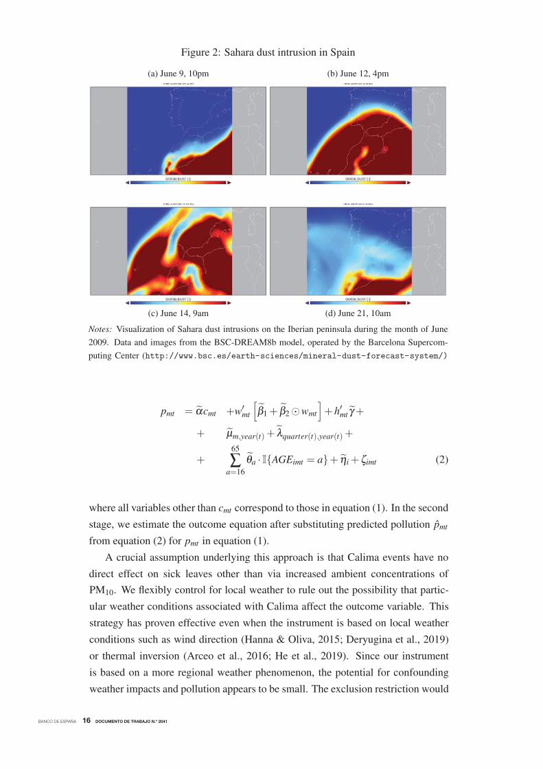
Figure 2 illustrates how Sahara dust traveled across different regions in Spain

during a Calima episode in June 2009. On June 9, the dust plume was building up


Figure 1: Average percentage share of Calima days per month

0

5

10

15

20

25

Cal

ima

days

[%]

1 2 3 4 5 6 7 8 9 10 11 12

Notes: Each bar represents the average percentage share of days in a given month classified as a

Calima episode, based on data from the Spanish Ministry for the Ecological Transition (2018).

over North Africa (Figure 2a). Three days later, the plume had extended to cover

the Canary Islands and Southern Spain, but not the Balearic Islands (Figure 2b). On

June 14, all of Spain was exposed to Sahara dust, though the intensity varied across

regions (Figure 2c). Figure 2d depicts the withdrawal of the dust cloud which was

completed at the end of June.

The influence of Sahara dust on ambient PM10 concentrations cannot be mea-

sured by regular air quality monitors. Therefore, the possible link between ambient

pollution and Calima is evaluated ex post using data from rural background mon-

itors and meteorological back-tracking models such as the one that generated the

data underlying Figure 2. The scientific procedure (Escudero et al., 2007; Querol

et al., 2013) behind this attribution is standardized across EU member states and

designed to ensure a level playing field across European cities when determining

whether they are in compliance with the EU standard for PM10 concentrations.

Because Calima events substantially increase non-anthropogenic PM10 concentra-

tions, the cities affected by this phenomenon are allowed to discount the measured

24-hour-mean concentration for this effect (see Appendix C for more details). Off-

ical PM10 discounts constitute a valid instrument for pollution because they shift

local PM10 concentrations in ways that are plausibly orthogonal to local conditions

that drive sick leaves, after conditioning on weather.

Specifically, denote by cmt the weekly share of days for which the city m’s

applicable PM10 discount is strictly positive (Calima days). The first-stage equation

for pollution is given by


where all variables other than cmt correspond to those in equation (1). In the second

stage, we estimate the outcome equation after substituting predicted pollution pmt

from equation (2) for pmt in equation (1).

A crucial assumption underlying this approach is that Calima events have no

direct effect on sick leaves other than via increased ambient concentrations of

PM10. We flexibly control for local weather to rule out the possibility that partic-

ular weather conditions associated with Calima affect the outcome variable. This

strategy has proven effective even when the instrument is based on local weather

conditions such as wind direction (Hanna & Oliva, 2015; Deryugina et al., 2019)

or thermal inversion (Arceo et al., 2016; He et al., 2019). Since our instrument

is based on a more regional weather phenomenon, the potential for confounding

weather impacts and pollution appears to be small. The exclusion restriction would

Figure 2: Sahara dust intrusion in Spain

(a) June 9, 10pm (b) June 12, 4pm

(c) June 14, 9am (d) June 21, 10am

Notes: Visualization of Sahara dust intrusions on the Iberian peninsula during the month of June

2009. Data and images from the BSC-DREAM8b model, operated by the Barcelona Supercom-

puting Center (http://www.bsc.es/earth-sciences/mineral-dust-forecast-system/)

pmt = αcmt +w′mt

[β1 + β2 �wmt

]+h′mt γ +

+ μm,year(t) + λquarter(t),year(t) +

+65

∑a=16

θa · I{AGEimt = a}+ ηi +ζimt (2)


also be violated if Calima changed behavior. A precondition for this is that workers

are aware of Calima while it lasts. On the Canary Islands, located 1,300 kilometers

to the south-west of the Iberian peninsula and just 115 kilometers off the Moroc-

can Atlantic coast, Sahara dust advection is frequent and sometimes visible, hence

awareness must be taken for granted. Although we cannot rule out behavioral

responses to Calima there a priori, robustness checks discussed in Section 5.2.3

below show that our results are not driven by workers from the Canary Islands. In

the rest of Spain, Sahara dust events are less frequent and less intense. We found

no evidence of the public being alerted to such events during our study period.

Finally, the exclusion restriction would be violated if PM10 originating from

the Sahara has a substantially different effect on human health than PM10 from

local sources. Specifically, if the chemical composition of PM10 from the Sahara

differed substantially from that of non-desert PM10, we should suspect that their

health impacts differ, too. Perez et al. (2008, Fig. 3) compare mass-adjusted con-

centrations of the four group elements in PM10 and find that crustal elements are

more frequent during Saharan dust days whereas carbon, secondary aerosols, and

marine aerosols show no difference. From a study of Madrid, Barcelona and eleven

other southern European cities, Stafoggia et al. (2016, p. 418) conclude that “the

health effects of dust-derived PM10 are of the same (or similar) magnitude as those

reported for anthropogenic sources of air pollution”. This lends support to our as-

sumption that the instrumental variable has no direct effect on human health except

through raising overall ambient PM10 concentrations.

4 Data

For the analysis in this paper, we merge several large datasets that are described in

more detail in this section.

4.1 Data sources

4.1.1 Employment histories

Our primary data come from the National Institute of Social Security which admin-

istrates both health insurance and pension benefits for more than 93% of the work-

force in Spain. Since 2004, the administration maintains a research dataset, the

Muestra Continua de Vidas Laborales, henceforth referred to as the MCVL (Span-

ish Ministry of Employment, Migration and Social Security, 2018). The MCVL

is a non-stratified random sample of anonymized individual work histories, cover-

ing approximately 4% of all individuals who were affiliated with social security at

some point during the reporting year. An individual record contains information


9Alba (2009) and Malo et al. (2012) have used linked MCVL and sick leave data before, but

only for a single year.

4.1.3 Air pollution

Data on air pollution were obtained from the Spanish Ministry for the Ecological

Transition (2016). These data are updated on a yearly basis and are also used within

the EU framework for reciprocal interchange of information and reporting on am-

bient air quality (2011/850/EU). The database is comprised of time series data on

ambient concentrations of a variety of air pollutants with up to hourly resolution as

well as meta-data on monitoring stations. For our analysis, we use readings taken

by 784 air quality measurement stations across Spain between January 2005 and

December 2014. Apart from location, these stations differ in terms of the set of

air pollutants they monitor and the time window of measurement. The vast major-

ity of stations remain active throughout the sample period. The meta-data report

the municipality where the measurement station is located. This allows us to link

them to construct a dataset of air quality across Spanish cities. When more than

one air quality station is located in a municipality, the readings are averaged across

stations.

on both current-year and historical employment relations, dating back to the time

when the administration began to keep computerized records.

4.1.2 Sick leaves

Information on sick leaves taken by social security affiliates is first gathered and

processed by the employer’s mutual indemnity association which relegates the

information back to the social security administration when reimbursements are

claimed. While sick leaves are not contained in the MCVL, the social security

administration has provided us with a customized dataset that merges individual

records of sick leaves to the MCVL during the years from 2005 to 2014. As a

result, we have a panel dataset containing daily observations of sick leaves taken

by 1.6 million individuals, the diagnosis code based on the International Statistical

Classification of Diseases and Related Health Problems (ICD), as well as informa-

tion on their employment status, wage, age, occupation, and many other character-

istics. To the best of our knowledge, we are the first team of researchers to analyze

this extraordinary dataset.9 A caveat is that the dataset is not well-suited to analyze

sick leaves taken by unemployed workers. This implies that the analysis to follow

has little to say about the impact of air pollution on the unemployed, and on severe

health consequences such as permanent disability or death.


4.1.4 Weather

Meteorological data were provided by the Royal Netherlands Meteorological In-

stitute (2019) as part of the European Climate Assessment & Dataset (ECA&D)

project. Within the ECA&D project, national meteorological institutes and re-

search institutions from 31 European countries collect daily data on twelve es-

sential climate variables. For Spain, historical information is available from 1896

onward. The number of variables and geographical coverage has been increasing

steadily until today. Based on a total of 193 geocoded weather stations, we assign

to each municipality the weather conditions at the station that is closest to the mu-

nicipality’s centroid and has non-missing data. Hence, the assigned weather station

is not necessarily located within the boundaries of the municipality.

4.1.5 Calima variables

We downloaded data on PM10 discounts from the website of the Spanish Ministry

for the Ecological Transition (2018). The data report daily PM10 discounts for 29

locations in Spain. We follow the official procedure and assign to each municipality

the closest station with available data (see Appendix C for more details).

4.1.6 Other controls

Factors such as epidemics, bank holidays, and school vacations likely affect an

individual’s propensity to call in sick. To the extent that these factors are correlated

with pollution, omitting them from the analysis might result in biased estimates.

We thus collected data to control for such factors.

Flu outbreaks are monitored and recorded by the Spanish center for disease

control (Instituto de Salud Carlos III) under the auspices of its flu surveillance

system (Sistema centinela de Vigilancia de la Gripe en Espana). Weekly data

for the flu incidence (number of cases per 100,000 inhabitants) are published for

each autonomous community,10 except Galicia and Murcia (Spanish Center for

Disease Control, Instituto de Salud Carlos III, 2016).11 We merge the flu data

to our estimation sample at the level of the Autonomous Community. In case of

missing observations, data were imputed using the national average.

The dates of school vacations and bank holidays vary at the levels of the au-

tonomous community, province, and even municipality. We gather this informa-

tion from the various regional “official bulletins” and numerous other sources. The

linking is done at the pertinent geographic level.

10Spain is not a federation, but a decentralized unitary state comprised of 17 autonomous com-

munities and two autonomous cities.11In a normal year, the monitoring is in place during the flu season, i.e. from week 40 until week

20 of the following year. In 2009, year-round surveillance was in place because of the swine flu.


4.2 Data cleaning

Our dataset contains daily records of individual sick leaves between January 1,

2005 and December 31, 2014. The raw sample is comprised of approximately four

billion worker-by-day observations over the full sample period. However, some

cleaning steps are necessary in order to use the sample for our purposes. This

subsection describes and justifies those steps.

First, we drop all workers living in municipalities with less than 40,000 inhab-

itants. For these workers, the place of residence is reported only at the level of the

province, which is too coarse for accurate spatial matching to pollution and weather

data. For all remaining workers, we know the place of residence at the five-digit

municipality code level which is required for matching. Since these muncipalities

have 40,000 inhabitants or more, we shall henceforth refer to them as cities. We

retain just over half of the workers in the raw sample after performing this step.

Second, we impose the following sample restrictions. We only keep worker-by-

day observations of individuals aged 16 to 65 who are actively employed and for

which we have information on employers and wages. Individuals who are reported

to have taken any sick leave of more than 550 days are dropped, as this number

exceeds the legal maximum duration. We also remove individuals with reported

employment relations after death, negative-length employment durations, as well

as duplicate or negative wages. Worker-by-day observations with inflation-adjusted

wages in the 99.5th percentile are also excluded.

Third, we drop observations with missing pollution data. In cities where pol-

lution measurements are derived from more than one air quality monitor, failure

to account for entry and exit of monitors would lead to incoherent time series. In

such cases, we drop all data from monitors reporting less than 120 days of PM10 in

any reporting year. If this leaves two or more monitors in the data, we require that

all monitors report in all years. Finally, we drop all observations on December 31

and January 1 because of the unusually high contamination levels that result from

fireworks during the new year’s festivities.

Following these cleaning steps, our sample contains between 231 thousand and

263 thousand workers per year who live in 99 cities spread across the Spanish

peninsula and the islands. Figure 3a displays a map with all cities included in the

estimation sample, and Figure 3b marks the location of each air quality monitor in

the sample. The 99 cities included in our sample are home to 55% of the Spanish

population and to 51% of all workers affiliated with the general regime of the social

security system.


4.3 Descriptive statistics

Our sample contains more than half-a-billion daily observations for 466,174 work-

ers aged between 16 and 65 years. To improve computational tractability, we ag-

gregate the data to the weekly level. The first panel of Table 2 provides summary

statistics at the worker level. The average propensity to take a sick leave in a given

week is 2.79%. The share of female workers is 46%. Figures B.1 and B.2 in Ap-

pendix B plot the duration of sick leaves and the frequencies of the main diagnosis

codes, respectively.

The remaining panels of Table 2 report descriptive statistics on pollution vari-

ables and other covariates, gathered at the city-by-week level. The second panel

summarizes the data on particulate matter. The average concentration of PM10 is

27 μg/m3, which is well below the EU annual standard of 40 μg/m3, but higher than

20 μg/m3, the limit value recommended by the World Health Organization (WHO,

2006). Non-anthropogenic PM10 contributes just 2.1 μg/m3 to this average value.

However, the maximum values show that the non-anthropogenic contribution to

PM10 is very important on high-pollution days. The share of days exceeding the

24-hour standard is 7%, and the share of Calima days is 15%. This means that not

every Calima day is a high-pollution day.

The third panel of Table 2 provides descriptive statistics for other air pollutants

(CO, SO2, NO2, and O3), and the fourth panel summarizes the weather variables.

Daily average temperature is measured in degrees Celsius, wind speed in 0.1 meters

per second, precipitation in 0.1 millimeters, and cloud cover in integer-valued oktas

ranging from 0 (sky completely clear) to 8 (sky completely cloudy). Sunshine is

measured in hours per day, humidity in percent and pressure in hectopascals. The

last panel of the table reports the flu rate, in cases per 100,000 inhabitants.

In some of the regressions below, we examine a possible nonlinear relationship

between health and air quality. Following Currie et al. (e.g. 2009a), we partition

the support of the distribution of pollution measurements at quartiles of the EU-

mandated daily limit value: zero to 50% of the limit, 50% to 75%, 75% to 100%,

100% to 125% of the limit, and above 125% of the limit. Table 3 reports the

percentage share of days in each partition. EU air quality standards were exceeded

for PM10 (with a frequency of 7.4%) and for O3 (with a frequency of 4.5%). The

concentrations for CO and SO2 hardly ever exceeded half of the respective daily

limit values.12 Since there is no daily EU limit for NO2, we construct bins for this

pollutant using the EU limit for annual average concentrations (40 μg/m3), which

12This is not to say that the ambient concentrations of carbon monoxide and sulfur dioxide are

innocuous. In fact, the World Health Organization has recommended much stricter air quality

standards than those prevalent in the EU in order to avoid health problems. Municipalities also

violated EU standards other than the ones listed here, such as the annual limit value for NO2.


Figure 3: Geographic coverage

(a) Cities in the sample

(b) Location of air quality monitors

Source: Own representation based on data from Database of Global Administrative Areas (GADM)

https://gadm.org/


Table 2: Descriptive statistics, 2005-14

Variable mean sd min max observations

1. Social security data (workers)Age 37.7 11.5 16 65 466,174

Female share [%] 46 49.8 0 100 466,174

Absence rate [%] 2.79 15.9 0 100 � 100 million

2. Particulate matter PM10 (city-by-week)Ambient concentration [μg per m3] 26.8 13.0 0.0 188.0 38,613

Concentration due to Calima event [μg per m3] 2.1 5.5 0.0 140.6 38,613

Days PM10 exceeds 24-hour standard [%] 7 19 0 100 38,613

Calima days [%] 15 25 0 100 38,613

3. Other air pollutants (city-by-week)CO [mg per m3] 0.5 0.3 0.0 5.2 25,279

SO2 [μg per m3] 5.5 4.9 0.0 121.6 29,529

NO2 [μg per m3] 25.7 14.7 0.0 140.8 33,421

O3 [μg per m3] 73.1 25.8 1.0 176.6 31,305

4. Weather data (city-by-week)Temperature [◦C] 15.9 6.4 -6.7 36.8 38,613

Wind speed [0.1 m/s] 29.4 15.2 0.0 142.9 38,613

Precipitation [0.1mm] 15.5 32.0 0.0 972.0 38,613

Cloud cover [okta] 3.9 1.8 0.0 8.0 38,613

Sunshine [h] 7.3 3.2 0.0 14.5 38,613

Humidity [%] 66.7 13.5 20.0 100.0 38,613

Pressure [hPa] 1,016.7 5.8 978.3 1,041.2 38,613

5. Flu prevalence (region-by-week)Flu rate per 100,000 inhabitants 47.1 86.9 0.0 1016.5 11,587

Table 3: Distribution of days per week by pollutant and percent of limit value

PM10 CO SO2 NO2 O3

[50;75) 26.2 0.0 0.1 22.9 41.0

[75;100) 11.5 0.0 0.0 14.9 23.3

[100;125) 4.3 0.0 0.0 8.8 4.2

[125,∞) 3.1 0.0 0.0 9.0 0.3

Notes: Each column reports the percentage share of days

per week with ambient concentrations for different quar-

tiles of the daily limit value stipulated by the EU. Limit

values refer to either 24-hour averages (for PM10 and

SO2) or maximum 8-hour averages (for CO and O3). For

NO2, the bins refer to daily averages evaluated against the

annual limit value, as the EU has not defined a daily limit

value. All limit values are reported in Table 1.


is exceeded on 17.8% of days. This number is reported for completeness and has

no immediate interpretation in the context of existing air quality regulations.

5 Results

5.1 Baseline estimates

Figure 4 plots weekly absence rates against ambient levels of PM10. Both the raw

data and the residualized data from an OLS estimation of equation (1) at the city-

level suggest that the relationship is positive and increasing. This is also born out

by the estimation results for regression equation (1). Table 4 reports OLS esti-

mates (in columns 1 and 4), IV estimates (columns 2 and 5), and respective first

stages (columns 3 and 6) for two alternative measures of air pollution.13 In the first

three columns, PM10 is measured as the share of days per week on which the daily

limit concentration of 50 μg/m3 is exceeded (PM10 exceedance). This identifies

the treatment effect of pollution using only high-pollution events. In columns 4

to 6, pollution is measured as average concentrations in μg/m3. If it was known

with certainty that the sick leave response is directly proportional to pollution con-

centrations, estimating a specification linear in PM10 would be more efficient as it

exploits variation in pollution over the entire support.

The IV regression is implemented as a two-stage-least-squares (2SLS) proce-

dure where local PM10 is first regressed on the Calima variable and controls. This

regression is reported in columns 3 and 6 of Table 4 for PM10 exceedance and

PM10, respectively, and shows that Calima is a strong predictor of ambient PM10

concentrations (R2 = 0.41 and R2 = 0.65, respectively). In the second stage, the

absence rate is regressed on the predicted PM10 variable and controls.

The association between pollution and sick leaves is positive and statistically

significant across all specifications, suggesting that higher levels of pollution lead

to more sick leaves. The IV estimates exceed the OLS estimates by a factor of 3.

This points to attenuation bias that could arise from measurement error in PM10 but

also due to other sources of bias that were discussed in Section 3.3 above. In the

analysis to follow, we thus focus on the IV estimator which allows for a causal inter-

pretation of the estimated relationship. The IV estimates of our baseline regressions

imply that, on average, a 10-percentage point reduction in the share of exceedances

of the limit value reduces the absence rate by 0.0213 percentage points, i.e. by

0.8% of the mean absence rate (0.0279). Furthermore, a reduction in average PM10

concentrations by 10 μg/m3 reduces the absence rate by 0.03 percentage points.

13The estimation of OLS and IV regressions with high-dimensional fixed effects is implemented

with the Julia programming language package FixedEffectModels.


Table 4: Baseline estimates for PM10

Weekly absence rate PM10 exceedance Weekly absence rate PM10

(1) (2) (3) (4) (5) (6)

PM10 exceedance 0.073*** 0.213***

(0.016) (0.067)

PM10 0.001*** 0.003***

(0.0004) (0.001)

Calima 0.194*** 15.5***

(0.022) (1.06)

Estimator OLS IV First-stage OLS IV First-stage

Observations 100,739,754 100,739,754 100,739,754 100,739,754 100,739,754 100,739,754

Mean outcome 2.79 2.79 0.08 2.79 2.79 28.04

R2 0.165 0.165 0.413 0.165 0.165 0.648

First-stage F statistic 80.6 216

Notes: Coefficients scaled by a factor of 100 for better readability. All regressions control for individual fixed effects, age fixed effects, city-

year fixed effects, year-quarter fixed effects, flu prevalence and include linear and squared terms of eight weather variables. Robust standard

errors in parentheses are clustered by city and by week. ∗p < 0.10, ∗∗p < 0.05, ∗∗∗p < 0.01.


5.2 Robustness checks

Notes: The figures show binned scatter plots after grouping all observations into 20 bins of equal

size based on the variable depicted on the x-axis. The dots represent the mean value for each

bin. The dashed line shows the predicted relationship based on an OLS estimation for the un-

derlying data. Subfigure (a) plots the relationship between PM10 and weekly absence rates at the

city-level. Subfigure (b) plots the relationship of the same variables, after controlling for city-year

fixed-effects, year-by-month fixed-effects, weather conditions, school holidays, other public holi-

days, and flu rates.

5.2.1 Dynamics

Our main regression equation relates sick leaves to contemporaneous pollution and

weather. Previous research has documented that air pollution can have dynamic

effects on worker productivity (He et al., 2019). To investigate this, we estimate

alternative specifications of equation (1) which include weekly lags of PM10 ex-

ceedance and use the respective lags of Calima as instrumental variables. The re-

sults, reported in Appendix Table A.2, show that the impact of air pollution on sick

leaves can last for up to two weeks. Compared to the specification without lags,

the contemporary effect of PM10 decreases in magnitude by about 15% but the

coefficient on the first lag is almost as large. Further lags do not matter empirically.

The lag distribution is open to more than one interpretation, however. When

interpreted as a dynamic treatment effect, it implies that a one-off shock to pollu-

tion affects health in the current and in the next week. The total effect would then

be given by the sum of both point estimates which amounts to twice the contempo-

raneous effect. Yet this could be confounded by high-pollution episodes that last

multiple days. For example, a four-day event can fall either into a single week or

extend over two subsequent weeks. In the former case, the event contributes only to

Figure 4: Sample correlation between sick leaves and PM10

(a) Binned scatter plot

2.7

2.8

2.9

3

3.1Ab

senc

e R

ate

10 20 30 40 50 60PM10

(b) Binned scatter plot residuals

−.04

−.02

0

.02

.04

Abse

nce

Rat

e R

esid

ual

−20 −10 0 10 20PM10 Residual


5.2.2 Non-linear effects of pollution

We shed light on the functional form of the pollution-health relationship by re-

estimating equation (1) using alternative thresholds to define a high-pollution event.

Appendix Table A.3 presents results for OLS and IV regressions where we use the

share of week days with pollution exceeding 50%, 75%, 100% (as in the baseline),

or 125% of the legal limit of 50 μg/m3 on a given day. The IV point estimates show

a clear pattern in that (i) higher threshold values for pollution lead to stronger in-

creases in the propensity to take a sick leave, and (ii) the increment in the sick leave

impact increases for constant increments in the pollution threshold. The implica-

tion is that a linear functional form, which has often been used in the literature,

would misrepresent the underlying pollution-health gradient in our application and

would lead us to underestimate the health hazard for the right tail of the pollution

distribution. The threshold-based approach we use throughout the remainder of

this paper circumvents this problem, though it averages over the impacts of high

and extremely-high pollution days.

To investigate whether pollution levels below the EU 24-hour standard have a

significant impact on sick leaves taken, we estimate a non-parametric version of

equation (1) where individual-by-week pollution exposures are sorted into 50 bins

of equal size.14 The share of days in the lowest quantile is omitted. The OLS

estimates for the different pollution bins are plotted in Figure 5. The grey area

represents the 95% confidence intervals of each indicator. For visual clarity, the

49 estimates and confidence intervals are connected by straight lines. The point

14We classify daily city-level PM10 into 50 quantiles after weighing each city-day by the number

of workers observed in the MCVL to account for different exposure profiles across cities. To avoid

a disproportionately large bin at the top, we drop PM10 readings in the 99.9th percentile. The 50

indicators for each bin are then averaged at the weekly level. Hence, the resulting variable indicates

the share of days in a given city and week in a particular bin. After matching the indicators to the

worker-level data, we estimate equation (1), replacing pmt by 49 indicators.

estimates are positive and increasing for values of 35 μg/m3 and higher, and they

become statistically significant at 46 μg/m3 just below the limit value.

identification of the coefficient on contemporaneous PM10, but in the latter case the

event also helps to identify the coefficient on lagged PM10. Our regression model

cannot disentangle the dynamic effects of two-day pollution event in the previous

week from the contemporaneous effects of four-day event that extends over both

the previous and current week. In the analysis to follow, we thus focus on the con-

temporaneous effect only. We acknowledge that this might underestimate the full

health impact.


Figure 5: Non-linear impacts of PM10 on sick leaves

Notes: The graph depicts point estimates for different bins of PM10 concentrations from an OLS

regression of sick leave on indicators for each bin and controls. The red line indicates the location

of the EU 24-hour standard for PM10. The grey areas indicate 95%-confidence intervals.

5.2.3 Exclusion of Canary Islands

The IV estimation rests upon variation in particulate matter due to Sahara dust

advection and transport. Because of their geographic proximity to the Sahara, the

Canary Islands are subject to this phenomenon more frequently and with greater

intensity than the rest of Spain. This could lead to a violation of the exclusion

restriction, e.g., if the local population change their behavior in response to Calima.

We therefore estimate the main specification after dropping all cities located on the

Canary Islands from the sample. Results reported in Appendix Table A.4 show that

the Canary Islands have no particular influence on the estimation results.

5.2.4 Non-linear regression model

Our baseline specification (1) fits a linear probability model to an outcome variable

that ranges only between zero and one. The model is thus necessarily mis-specified,

but it has the enormous benefit of allowing us to implement high-dimensional fixed-

effects and IV estimators in straight-forward ways. Since the realizations of the

outcome variable – the share of sick leaves at the city-by-week-level – takes val-

ues between 0.38% and 7.02%, we reckon that the bias due to misspecification

is not large enough to give up the simplicity and computational tractability of the

linear model. We investigate this by estimating a logit model with fractions and

worker fixed effects as a non-linear alternative model. This alternative has its own

drawbacks as it does not accommodate instrumental variables and, in general, the

inclusion of individual fixed effects gives rise to an incidental parameters prob-


lem.15 Results reported in Appendix Table A.5 show that the average marginal

effect for the PM10 exceedance of 0.063 is smaller than but very close to the OLS

baseline estimate of 0.073, while for the PM10 in levels, the average marginal effect

of 0.001 is almost equivalent to the OLS baseline estimate.

5.3 Estimates by ICD-9 diagnosis group

For a subset of absence spells we observe diagnoses, coded according to the Ninth

Revision of the International Statistical Classification of Diseases (ICD-9). This

classification scheme subdivides diseases and health-related problems into 17 main

categories, referred to as chapters. The three most commonly diagnosed ICD-9

chapters in our sample are “VI: diseases of the musculoskeletal system”, “V: mental

disorders”, and “XVII: injury and poisoning”, as reported in Appendix Table B.3.

Table 5 reports estimates of 17 IV regressions, using as the dependent variable in

equation (1) the chapter-specific absence rate. In those regressions, we drop (i) all

spells for which the ICD-9 code is not reported and (ii) all spells with a diagnosis

different from the diagnosis group used in the definition of the respective dependent

variable, which accounts for the fact that diagnoses are mutually exclusive.16

The strongest effect of PM10 on sick leaves is found for the diagnosis chapters

XVI and V. The former stands for “symptoms, signs and ill-defined conditions” and

includes headaches, tachycardia (elevated heart rate), apnea (cessation of breath-

ing), or nausea, among others. The latter (mental disorders) includes, among oth-

ers, symptoms related to dementia and depression, which have been linked to air

pollution in recent research (Bishop et al., 2018; Braithwaite et al., 2019; Fan et al.,

2020). A positive effect also emerges for chapter VI (diseases of the nervous and

15When the panel is short (T small), noisy estimates of the fixed effects contaminate the esti-

mates of the common parameters and the marginal effects due to the nonlinearity of the model. In

particular, the magnitude of the bias of the maximum likelihood estimator would be on the order of

1/T . However, given that we use weekly data, the average number of observations per worker in

our sample is 217.7, suggesting that the incidental-parameter bias will be very small. Simulations

by Fernandez-Val (2009) show that the size of the bias is already small when T = 16.16Appendix Table A.6 reports the results from an alternative regression where chapter-specific

absences are set to zero whenever (i) no diagnosis is reported or (ii) an ICD-9 code does not belong

to the diagnosis chapter defining the dependent variable. The results are almost identical to the ones

reported in Table 5.

sense organs) which includes Alzheimer’s disease, migraine, and eye disorders. In

addition, we find a small but statistically significant negative effect for the chapter

“diseases of the blood and blood-forming organs”. We refrain from a causal inter-

pretation of this point estimate because it is based on very few observations: Less

than 0.3% of all sick leaves are classified in this chapter (vs. 11.6%, 13.5%, and

4.2%, respectively, for the above-mentioned diagnosis chapters; cf. Table B.3). In-

terestingly, we do not find statistically significant effects when looking at diagnosis


chapters for respiratory diseases (which includes asthma, bronchitis, and chronic

obstructive pulmonary disease) or cardiovascular diseases.17

6 Heterogeneity of treatment effects

The richness of our data allows us to investigate the heterogeneity of treatment

effects with respect to a wide variety of characteristics of workers and jobs. To

do so, we define for each characteristic a categorical variable and split the sample

accordingly. In this way, we accommodate heterogeneous reactions not only to

air pollution but also to any other variable specified in regression equation (1).

First, we analyze heterogeneity with respect to worker characteristics. Next, we

study how workers in different occupations react to air quality. We conclude the

examination of heterogeneous treatment effects comparing workers with different

initial health stocks.

6.1 Heterogeneity across workers

Gender

When splitting the sample by gender, the point estimates are larger for female

workers than for male workers (cf. Appendix Table A.7). A 10-percentage point

reduction in the share of PM10 exceedances reduces the absence rate by 0.026 per-

centage points for women and 0.017 percentage points for men. However, taking

into account the mean absence rates for each group (3.41% for females, and 2.25%

for males), the relative effect is 0.8% in both cases.

17We can only speculate about the reasons for this. It could be that patients with asthma or

respiratory symptoms are more likely to self-medicate in response to a pollution shock, in particular

when they know that they have the disease. Bias could also arise due to the fact that ICD codes are

not available for all sick leaves, or due to systematic differences in the reporting quality, depending

on whether patients were treated in the emergency room or by their general practicioner.

Age

Appendix Table A.8 reports the regression results after subdividing workers into

three age groups of approximately equal size. The point estimates increase with

age among young and middle-aged workers. For workers older than 45 years,

the increment in the OLS point estimate is less pronounced and the higher mean

absence rate in this group implies that the relative impact of high-pollution events

is as low as in the group of young workers. When interacting PM10 exceedances

with worker age we estimate that an additional year increases the pollution impact

on absences by 2.8% of the main effect (cf. Appendix Table A.9)


Table 5: Effects of PM10 on ICD-9 Diagnosis Groups

PM10 exceedance Mean N

I: Infectious and Parasitic Diseases 0.002 0.067 97,528,520

(0.007)

II: Neoplasms 0.004 0.097 97,511,232

(0.005)

III: Endocrine, Nutritional andMetabolic Diseases, and Immunity Disorders

0.001 0.019 97,432,211

(0.001)

IV: Diseases of the Bloodand Blood-forming Organs

-0.001*** 0.007 97,417,805

(0.000)

V: Mental Disorders 0.038*** 0.302 97,730,323

(0.009)

VI: Diseases of the Nervous Systemand Sense Organs

0.015** 0.096 97,523,735

(0.007)

VII: Diseases of the Circulatory System 0.001 0.091 97,507,524

(0.002)

VIII: Diseases of the Respiratory System 0.008 0.137 97,624,631

(0.012)

IX: Diseases of the Digestive System 0.010 0.101 97,535,500

(0.007)

X: Diseases of the Genitourinary System -0.004 0.054 97,474,571

(0.004)

XI: Complications of Pregnancy, Childbirth,and the Puerperium

0.003 0.080 97,498,058

(0.003)

XII: Diseases of the Skinand Subcutaneous Tissue

-0.001 0.026 97,441,348

(0.003)

XIII: Diseases of the Musculoskeletal Systemand Connective Tissue

0.020 0.596 98,073,192

(0.019)

XIV: Congenital Anomalies -0.000 0.006 97,416,810

(0.001)

XV: Certain Conditions originatingin the Perinatal Period

0.001 0.001 97,412,186

(0.000)

XVI: Symptoms, Signsand Ill-defined Conditions

0.042*** 0.282 97,745,795

(0.011)

XVII: Injury and Poisoning 0.017 0.289 97,733,701

(0.012)

Notes: Rows report the IV point estimates for PM10 exceedance in separate regressions where (i)

the dependent variable is defined on sick leaves with a diagnosis from the ICD-9 chapter indicated

in column 1 and (ii) all sick leaves with a diagnosis from another chapter are dropped. Coefficients

scaled by a factor of 100 for better readability. All regressions control for individual fixed effects,

age fixed effects, city-year fixed effects, year-quarter fixed effects, flu prevalence and include linear

and squared terms of eight weather variables. Robust standard errors in parentheses are clustered by

city and by week. ∗p < 0.10, ∗∗p < 0.05, ∗∗∗p < 0.01.

Presence of dependent children

Differences in sick-leave taking across workers could be related to the presence

of dependent children in the household. We explore this in Appendix Table A.10


which reports the treatment effects estimated separately for workers with and with-

out children under age twelve in the household.18 We find that the point estimates

are very similar in both groups. The differences are well within the margin of error

and, relative to the mean absence rates, the treatment effect is around 0.8% in both

groups.

This contrasts with the evidence provided by Aragon et al. (2017) that Peruvian

workers with dependent children are more likely to reduce their labor supply during

high-pollution episodes in order to take care of their children when air pollution

makes them sick. While it is plausible that caregivers in our sample stay at home

when their child is sick, such leaves are unlikely to be registered as a sick leave

taken by the parent. This is because Spanish labor regulations grant parents at least

two days of paid leave per year when a minor child is sick. Unfortunately, we

cannot investigate this further as we do not have information on such leaves.

Income and skills

Differences in income might induce heterogeneity in the treatment effects for a va-

riety of reasons. Workers with higher income may attach a higher value to health,

they might have access to better health care and more expensive medication, better

options to avoid air pollution, or benefit from a collective agreement that comple-

18Age twelve is the threshold used in Spanish labor regulations for granting work-hour reductions

or leaves for child rearing.

ments sick pay from the social security system. The overall effect of these and

other income-related factors on the estimated impact is ambiguous from an ex ante

perspective.

The reporting of income is not very precise in our dataset because contribution

bases are bottom and top coded. Therefore, we explore the treatment heterogeneity

with respect to skill groups that are highly correlated with the salaries that workers

received. The Spanish social security system classifies occupations into ten groups,

three of which can be considered as high-skilled (Bonhomme & Hospido, 2017).

When estimating the treatment effects separately for high-skilled and low-skilled

workers, the point estimates, reported in Appendix Table A.11, barely differ.

6.2 Heterogeneity across occupations

Sector affiliation

We begin our investigation of treatment heterogeneity across jobs with a compar-

ison across sectors. To this end, we split up the sample into nine sectors and esti-

mate equation (1) for each sub-sample. Figure 6 displays the mean absence rates

along with the point estimates for PM10 exceedance (see Appendix Table A.12 for

detailed sector definitions and estimation results).


Three findings emerge from this exercise. First, the estimated impact of high-

pollution events on sick leaves is positive in all sectors, and the relationship is

statistically significant in all sectors but agriculture. Second, there is meaning-

ful variation in the magnitude of these effects across sectors, with OLS estimates

ranging from 0.03 to 0.11 (compared to 0.07 in the full sample) and IV estimates

from 0.14 to 0.36 (compared to 0.21 in the full sample). Third, the mean per-

centage absence rate across sectors is quite heterogeneous and ranges from 1.83 in

the information and communication technologies (ICT) sector to 3.71 in the public

sector.

Such differences in mean absence rates could arise exclusively because of dif-

ferences in job characteristics, but in reality they are likely driven also by selec-

tion. All else equal, a worker with frail health prefers a job that doesn’t expose

her to high levels of air pollution or that comes with generous sick leave benefits.

Sorting on those characteristics is likely to induce bias in previous, cross-sectional

estimates of the impact of air pollution on work days lost (Ostro, 1983; Hausman

et al., 1984; Hansen & Selte, 2000). Since we have worker fixed-effects, our esti-

Figure 6: Heterogeneous pollution impacts across sectors

0 1 2 3 4

Public sector

Manufacturing

Professional services

Trade

Other services

Construction

Agriculture

Finance

ICTAbsence rateIV estimateOLS estimate

Notes: The chart displays mean absence rates, OLS estimates and IV estimates separately for the following sectors: Informa-

tion and communication technology (ICT), financial services, agriculture, construction, other services, trade, professional

services, manufacturing, and the public sector. All coefficients and absence rates have been multiplied by 100 for better

readability. The full results are reported in Appendix Table A.12.

mates are purged of selection bias. Nonetheless, the heterogeneity in the sectoral

estimates reflects the joint influence of these and other factors on the decision to

take a sick leave. For an illustration, consider the results for the ICT and the public


sector. The IV point estimates for these two sectors – 0.355 and 0.301, respectively

– are at the top of the range of estimated treatment effects. However, workers

in ICT exhibit the lowest average absence rate whereas public sector employees

have the highest. This suggests that selection on health cannot alone explain all

of the heterogeneity in treatment effects. While the cross-sector comparison of

treatment heterogeneities provides clues for the mechanisms driving them, pinning

down such mechanisms requires further analysis.

In the remainder of this section, we undertake such an analysis focusing on the

role of job security. This is motivated by the fact that both mean absence rates

and treatment effects are particularly high in the public sector, where employees

enjoy very high levels of employment protection – in particular, civil servants.

Compared to workers with low levels of job security, public sectors workers might

be more willing to take a sick leave when experiencing a negative health shock

because they do not have to fear any consequences for the continuation of their

tenure.19 In contrast, in sectors where precarious employment conditions are more

prevalent, such as agriculture and services, workers might take fewer leaves in

order to avoid repercussions on the likelihood of remaining employed. Since we

cannot rule out that confounding factors other than employment security drive the

cross-sector comparison, the subsequent analyses cut the data in different ways to

shed more light on this mechanism.

Employment protection in a dual labor market

The Spanish labor market features stark differences in employment protection be-

tween temporary and permanent employment contracts. Previous work has shown

that this dual labor market affects unemployment, job flows, productivity and wel-

fare (Dolado et al., 2002, 2005; Cabrales et al., 2014; Bentolila et al., 2019). It is

conceivable that differences in employment protection could affect the generosity

of sick leave benefits (e.g., at the level of collective bargaining) or the worker’s

willingness to take advantage of those benefits.

We investigate this by splitting the sample into three groups with increasing

degree of employment protection: temporary contracts, permanent contracts, and

civil servants. The results for each group are reported in Table 6. The IV point

estimates imply that, on average, a 10-percentage point reduction in the share of

exceedances of the limit value reduces the absence rate by 0.0155 percentage points

for workers with a temporary position, and 0.0202 percentage points for workers

with a permanent contract. Given the mean absence rates for each group (2.2%

for temporary, and 2.9% for permanent), the reaction is similar for both groups

(0.7%). However, the implied reaction for civil servants is larger both in absolute

19In addition, until July 2012, the replacement rates for the daily subsidy were substantially more

generous for workers in the public sector than in other sectors.


terms (0.0497 percentage points) and relative to the mean (1.2%), corroborating

the view that the propensity to take a sick leave in this group is not only higher on

average but also in response to pollution shocks.

Unemployment risk

Next, we use rich data on individual-level attributes in order to tease apart the po-

tential effect of unemployment risk from other factors driving a worker’s decision

to take advantage of sick leave benefits when pollution spikes. Unemployment risk

might matter for the following reason. If a worker fears that the frequency of her

sick leaves will be taken into account when her employer decides on whether or

not to retain her in the event of a mass layoff, it may be rational for her to not take

a sick leave even when sick. This is a testable prediction because we can estimate

individual unemployment risk from our data and relate this to the propensity to take

a sick leave.

In order to predict individual unemployment risk we fit a logit model for the

probability of losing a job in a given month for each of the nine sectors above.

All regressions control for gender, year, age, age squared, tenure, tenure squared,

experience, experience squared, nationality, and province of residence.20 Using

fitted regressions for each sector, we predict the individual unemployment risk for

20This approach is inspired by the labor literature. For example, Card (1996) uses predicted

wages as a proxy for skills in order to study the impact of unions on workers with different skill

levels. As the MCVL contains only limited information on unemployment status, we use missing

employment entries in the dataset as proxies for job loss. Since some workers exit the MCVL

sample at the end of the year, we include a dummy for the month of December which allows us to

control for this effect when predicting job loss. See Appendix D for details.

the first week in which a worker is observed. We then assign workers to one of

two groups, depending on whether this prediction lies above or below the sector’s

median risk. The assignment is made once for the worker’s entire time series. In so

doing, we capture time-invariant heterogeneity in a worker’s risk of job loss while

avoiding possible feedbacks of air quality on employment risk. We derive two

insights from this classification (summarized in results reported in Appendix Table

A.13). First, the average propensity to take a sick leave is lower among those facing

a higher risk of losing their job. Second, the increase in this propensity in response

to a high-pollution event is higher in the low-risk group than in the high-risk group,

an effect that holds in both relative and absolute terms.

We further analyze this using continuous variation in predicted unemployment

risk. Table 7 reports regression results from a variant of equation (1) that includes

the interaction of PM10 exceedance with the individual unemployment risk, stan-

dardized relative to other workers in the same sector. The IV coefficient implies

that a one-standard deviation decrease in individual unemployment risk is associ-

ated with an impact of pollution on sick leaves that is 43% higher.


Table 6: Treatment effects by contract type

Temporary contract Permanent contract Civil servants

(1) (2) (3) (4) (5) (6)

PM10 exceedance 0.069*** 0.155*** 0.066*** 0.202*** 0.137** 0.497***

(0.026) (0.059) (0.018) (0.074) (0.058) (0.189)

Estimator OLS IV OLS IV OLS IV

Mean outcome 2.238 2.238 2.850 2.850 4.321 4.321

Observations 25,786,038 25,786,038 67,323,069 67,323,069 7,055,193 7,055,193

R2 0.191 0.191 0.181 0.181 0.180 0.180

First-stage F statistic 86.511 79.280 67.395

Notes: Coefficients scaled by a factor of 100 for better readability. All regressions control for individual fixed effects,

age fixed effects, city-year fixed effects, year-quarter fixed effects, flu prevalence and include linear and squared terms of

eight weather variables. Robust standard errors in parentheses are clustered by city and by week. ∗p < 0.10, ∗∗p < 0.05,∗∗∗p < 0.01.

Table 7: Treatment effects by unemployment risk - interaction

Weekly absence rate

(1) (2)

PM10 exceedance 0.072*** 0.212***

(0.016) (0.066)

PM10 exceedance × unemployment risk -0.019* -0.092***

(0.010) (0.032)

Estimator OLS IV

Mean outcome 2.798 2.798

Observations 100,199,483 100,199,483

R2 0.165 0.165

First-stage F statistic 34.901

Notes: Coefficients scaled by a factor of 100 for better readability. All regressions con-

trol for individual fixed effects, age fixed effects, city-year fixed effects, year-quarter

fixed effects, flu prevalence and include linear and squared terms of eight weather vari-

ables. Standardized within-sector unemployment risk is also interacted with weather

variables, city-year dummies and year-quarter dummies. Robust standard errors in

parentheses are clustered by city and by week. ∗p < 0.10, ∗∗p < 0.05, ∗∗∗p < 0.01.

Our findings imply that estimates of the health damages of air pollution derived

from sick leave data may be underestimating the true health effects if workers in

jobs with low job security go to work despite being sick. In Section 7 we estimate

the magnitude of this divergence for all of Spain.


6.3 Heterogeneity with respect to health status

A long-standing interest in research on the pollution-health gradient has been with

the impact on particularly vulnerable individuals. In fact, much of the literature

approaches the topic with a focus on vulnerable populations such as infants (Currie

et al., 2014) or the elderly (Deryugina et al., 2019).

Thanks to having rich data on workers’ health records, we can go beyond the

current state of the literature and identify vulnerable individuals in a representative

sample of workers aged 16 to 65. To this end, we first construct a straightforward

indicator of health as the share of days missed due to the sick leaves taken during

the first twelve months that a worker is observed in the sample. We then estimate

a variant of equation (1) where PM10 exceedances are interacted with this health

measure.21

Table 8: Treatment effects by health status

Weekly absence rate

(1) (2)

PM10 exceedance 0.082*** 0.157*

(0.018) (0.087)

× absence share 0.578 2.578***

(0.354) (0.698)

Estimator OLS IV


Observations 74,706,090 74,706,090

R2 0.176 0.176


Notes: Coefficients scaled by a factor of 100 for better read-

ability. All regressions control for individual fixed effects,

age fixed effects, city-year fixed effects, year-quarter fixed ef-

fects, flu prevalence and include linear and squared terms of

eight weather variables. Robust standard errors in parenthe-

ses are clustered by city and by week. ∗p < 0.10, ∗∗p < 0.05,∗∗∗p < 0.01.

21In this estimation, we drop the first 18 months of a worker’s record to ensure that the spells

used to define vulnerability do not extend into the estimation period (a sick leave can last up to six

Table 8 reports the results. We find that the interaction term is positive and

statistically significant in the IV estimation but not for OLS. Two statistics from

the distribution of the absence share are helpful to further interpret these results.

First, the healthiest 76.5 percent of workers have an absence share of zero. Hence

months) and thereby have a direct effect on the estimation results.


this group responds to high-pollution events according to the main effect. Since the

main effect is positive and significant in the OLS regression, but not the interaction

effect, attenuation bias due to measurement error seems to be particularly severe

for workers with poor health.

Second, we define as vulnerable workers the ones in the top five percent of

the absence share distribution who missed at least 12.3% of work days due to ill-

ness. The IV estimates imply that the impact of high-pollution events on vulnerable

workers is more than 3 times higher than the effect on healthy workers. Therefore,

the mean effect masks large effects for particularly vulnerable individuals, a result

that has been established thus far only for populations either younger or older than

the working-age subjects we consider in our analysis. In further results reported in

Appendix Table A.14, we find that the discrepancy between healthy and vulnera-

ble workers is weaker when defining vulnerability based on the length of previous

sick leaves.22 This is consistent with the interpretation that especially workers with

chronic conditions but not excessively long sickness spells are harmed by air pol-

lution.

Our results complement the available evidence to support the claim that air

pollution imposes a disproportionately large health burden on vulnerable groups

of society. Our focus on sick leaves and workers also highlights the perhaps less

appreciated fact that universal sickness insurance with a benefit scheme for tempo-

rary disability helps to alleviate unequal distributional impacts of air pollution by

granting affected workers both access to treatment and time to heal.

7 Aggregate benefits of air quality improvements

The estimation results allow us to compute a lower bound on the benefits of im-

proving urban air quality in Spain. We proceed in two steps. First, we calculate the

reduction in sick days caused by a specific improvement in air quality. To translate

22In particular, the effect size ratio between lower 75 percent and top 5 percent of the distribution

is 2.5 when the health indicator is based on the maximum length and 1.2 when it is based on the

mean length.

this into a monetary benefit, we then multiply this number by the average daily

producer wage across workers. Under the assumption that workers are paid their

marginal product, this approximates the value of incremental production enabled

by the reduction in sick days. While improving air quality yields sizable additional

benefits by reducing mortality, human suffering, and medical treatment costs, we

focus on foregone production because this component of the social costs of air pol-

lution is directly linked to our outcome variable and has not yet been quantified in

previous research.


We start by considering a counterfactual intervention that enforces strict com-

pliance with the 24-hour standard for PM10 throughout the sample period. The

average share of worker days on which PM10 exceeded the EU limit value was

8.11% between 2005 and 2014. The IV point estimate implies that reducing this

share to zero would lower the absence rate by 0.017 percentage points (0.624% of

the mean). Specifically, we calculate the increase in work attendance as

Δ = 0.0811 ·7 ·0.00213 ·6,867,199 = 8,304 worker days per week

where the product of the first two terms yields the expected reduction in high-

pollution days per week, the third term is the IV coefficient and the last term is

Table 9: Productivity benefits of reducing PM10 exposure in urban Spain

I. Enforcement of 24-hour standards at II. Reduced exposure

50μgm3 37.5

μgm3 to > 50

μgm3 since 2005

Weekly Annual Weekly Annual Cumulative

absence production absence production absence production

[days] [AC million] [days] [AC million] [days] [AC million]

Baseline -8,304 39.31 -12,955 61.32 -5.55m 503

± 5,107 ± 24.18 ± 8,570 ± 40.57 ± 3.42m ± 309

Adjusted for -11,657 55.18 -18,536 87.74 -7.80m 706

job security ± 6,433 ± 30.45 ± 11,161 ± 52.83 ± 4.30m ± 389

Notes: Panel I reports counterfactual productivity benefits of strictly enforcing 24-hour standards for PM10 in

terms of reductions in (i) work days lost per week and (ii) incremental production. Counterfactual air quality

improvements are calculated relative to the observed PM10 concentrations in each city contained in the sample,

weighted by the number of social security affiliates in that city. Enforcing a limit of 50 μg/m3 is binding on

8.11% of worker days in the sample whereas a limit of 37.5 μg/m3 is binding on 20.73% of days. Panel II

reports the cumulative benefits of reductions in worker exposure to daily PM10 concentrations of 50 μg/m3 or

more that have actually occurred in urban Spain since 2005.

the average number of social security affiliates in our sample of 99 cities over the

period. We multiply this number with the daily producer wage in constant 2018

Euros, averaged across workers and years23 to obtain annualized benefits of

Ω = 52 · Δ · C 91.0 = C 39.31m.

To account for sampling error we include 95% confidence bands for all counterfac-

tual calculations reported in Panel I of Table 9.

Our IV estimate is based on a binary indicator for high-pollution events. In

the above exercise, this implies an assumption that PM10 concentrations below

23Averaging wages and employment across years is intended to dampen the impact of economic

fluctuations on the benefit estimates. As shown by Figure 7 below, such fluctuations were substantial

during the ten-year sample period.


50 μg/m3 are not harmful to human health. Yet the non-parametric OLS estimates

displayed in Figure 5 suggest that pollution increases absence rates even at lower

PM10 concentrations of less than 40 μg/m3. We thus repeat the calculations for a

scenario that enforces strict compliance with 75% of the PM10 limit value through-

out the sample period. This new standard would be binding for 20.73% of worker-

days. Using the IV estimate for exceedances above 37.5 μg/m3 (reported in Table

A.3), we compute a reduction in the absence rate of 0.027 percentage points and

an increase in work attendance by 12,955 days per week. The annual benefits in

terms of foregone production amount to C61.32 million, which is a 56% increase

compared to merely enforcing the EU limit value. Hence, the additional benefits of

improving air quality beyond the current EU standard for PM10 would be econom-

ically significant.

According to our results, high-pollution events cause an increase in sick leaves,

but this effect is significantly lower among workers facing a high risk of job loss

relative to the sector average. If those workers go to work despite being sick we

underestimate the burden of air pollution. To gauge how sensitive our benefit esti-

mates are to such presenteeism, we repeat the above calculations after eliminating

idiosyncratic unemployment risk. That is, we replace each worker’s estimated un-

employment risk by the smallest risk observed in the sector and predict the sick-

leave response based on the IV estimates reported in Table 7 which allow for dif-

ferential responses to pollution depending on unemployment risk. The results for

the two counterfactual scenarios are reported in the bottom row of Table 9. This

exercise shows that correcting for presenteeism leads to benefit estimates that are

more than 40% higher than in the baseline.

With these concepts in mind, we turn to evaluating the benefits of actual air

quality improvements that have taken place in urban Spain between 2005 and 2014.

Figure 7a shows a strong decline in worker exposure to PM10 concentrations ex-

ceeding the EU 24-hour limit (or 75% of that limit). In our sample of 99 cities, the

share of worker-weighted days with PM10 concentrations in excess of 50 μg/m3

declined from 18.8% in 2005 to just under 2% in 2014.24 The cumulative bene-

fit of this development is a reduction in work days lost by 5.55 (± 3.42) million

which would have resulted in foregone production worth C503 million (± C309

million). We calculate these numbers by computing for each year from 2006 on-

wards the reduction in PM10 exposure relative to 2005 and summing the associated

benefits across years in the sample. It is important to note that this calculation

is affected quite strongly by major economic fluctuations that occurred during the

sample period, depicted in Figure 7b. The years 2005 to 2007 were the final years

of a massive construction boom in Spain, with strong growth in both employment

24This improvement is in line with a broader pattern observed in the G7 countries, where the

mean population exposure to PM2.5 fell by 25% between 1990 and 2017 (OECD, 2019).


and producer wages. The financial shock and grand recession of 2008 triggered a

prolonged economic crisis in Spain which caused dramatic declines in those vari-

ables from 2009 onward. If we used 10-year averages of employment and wages

to compute benefits as in the counterfactual simulations above, we would likely

Figure 7: Trends in Pollution, Employment, and Wages 2005-2014

(a) Share of high-pollution days

0.1

.2.3

.4

2006 2008 2010 2012 2014Year

PM10 > 50 μg/m³PM10 > 37.5 μg/m³

(b) Employment and producer wages

8590

9510

0E

uros

of 2

018

66.

57

7.5

Milli

on w

orke

rs

2006 2008 2010 2012 2014Year

Affiliated workers (cities in the sample)Real daily producer wage

Notes: Figure a) displays the share of worker days with PM10 concentrations exceeding the EU 24-hour limit of 50 μg/m³

(solid line) and the share of worker days with concentrations in excess of 75% of the limit value (dashed line). The figure is

based on our sample of 99 Spanish cities with at least 40,000 inhabitants. PM10 concentrations are weighted by the number

of social security affiliates in each city and year. Figure b) displays the number of workers affiliated with the General Social

Security Regime on our sample of 99 Spanish cities with at least 40,000 inhabitants (solid line) and the daily producer wage,

expressed in constant 2018 Euros (dashed line).

overestimate the value of foregone production because air quality improvements

were largest during the crisis years. We account for this by using annual values.

As above, one can adjust the estimated benefits of air quality improvements to

account for presenteeism in the impact estimates. This yields a reduction in work

days lost by 7.80 (± 4.30) million and a corresponding increase in production worth

C706 million (± C389 million). Irrespective of which number one prefers, this ex-

ercise shows that the productivity-related benefits of air quality improvements that

occurred in Spain between 2005 and 2014 were both economically and statistically

significant.

8 Discussion and conclusions

We have conducted the first nation-wide study of the impact of air pollution on

work absenteeism. Our application is based on a representative panel of urban

workers affiliated with the Spanish social security system. Using naturally occur-

ring variation in Sahara dust advection to instrument for ambient concentrations of

PM10 we have estimated causal relationships that give rise to a number of policy

implications.

First, higher PM10 concentrations lead to more work absences, in particular for

levels of pollution that exceed the EU-mandated 24-hour limit value of 50 μg/m3.


This effect is economically significant even when sick leaves are valued only with

the foregone production during work days lost, a lower bound on the full social

costs which also include cost components related to loss of life, human suffering,

and medical treatment. The implication is that policies aimed at reducing particu-

late matter have non-negligible health benefits that are not accounted for in a sizable

literature focusing on severe morbidity and mortality outcomes. Our findings also

underline that air pollution damages human health for a broad range of symptoms

and diagnosis chapters.

Second, our findings corroborate that air pollution control is needed in partic-

ular to protect vulnerable members of society, a policy implication first derived

in previous research on infants and the elderly. Our analysis has contributed new

evidence for the working population by showing that workers in bad health suffer

disproportionately from air pollution. From a public policy perspective, protecting

the vulnerable is imperative on the grounds that there are no good substitutes for

health. In such a setting, monetary compensation is a blunt instrument for mitigat-

ing unequal welfare effects of environmental externalities.

Third, we establish that workers who suffer an adverse health shock due to air

pollution are less likely to take a sick leave the higher their individual risk of job

loss. As a consequence, such workers might fail to seek adequate treatment for

their diseases. This would likely decrease their productivity in the short run and

might also have detrimental health consequences in the long run.

We note several caveats. Our study is based on data from the social security

system which covers most but not all workers in Spain. Our results may thus not be

representative of self-employed, unemployed and permanently disabled workers.

Further data limitations imply that our results may not be representative for workers

in rural parts of the country.

A cautionary note is due in regards to the use of OLS vs. IV estimates when

deriving policy implications. Although our use of high-dimensional fixed effects

is well-suited to control for non-random assignment of air pollution in an OLS

regression, mismeasured pollution exposure likely causes attenuation bias in our

application. Our discussion of the results has predominantly relied on the IV esti-

mates because they mitigate this bias. However, their validity requires that PM10

originating from Sahara dust advection affects sick leaves only by shifting local

PM10 concentrations, conditional on weather and other controls. Based on the ev-

idence available to us, we have argued that violations of the exclusion restriction

are unlikely to drive our results. We note, however, that our interpretation of the IV

coefficient as a dose-response relationship for urban PM10 concentrations is based

on the premise that the pathological effects of PM10 blown in from the Sahara are

identical to those of urban PM10. Previous research on this topic documents small

but measurable differences in the chemical and mineralogical composition of those


variables (Perez et al., 2008), but also suggests there are no differential health im-

pacts (Stafoggia et al., 2016). We are aware that this does not constitute ultimate

proof of identical health effects. Nonetheless, it lends empirical support to an as-

sumption that allows us to derive valuable, additional insights from our empirical

results. In making this assumption, we trade-off the remaining scientific uncer-

tainty against the benefits of having point estimates that are not only purged of

attenuation bias but also interpretable as dose-response relationships for PM10.25

Should future research produce new evidence that makes the exclusion restriction

25The latter benefit would not arise if we used alternative IVs suggested in the literature which

shift several air pollutants at a time.

untenable, this would call for a reassessment of this trade-off and might suggest the

adoption of an alternative IV strategy. Even in such a scenario, however, our empir-

ical framework still provides intent-to-treat estimates suitable for evaluating work

days lost due to long-range transport of desert dust, which might become more

relevant as the problems of global climate change and desertification worsen.26

A final caveat to be addressed here concerns the measurement of foregone pro-

duction due to sick leaves. We have proposed two alternative measures. The first

measure only counts sick leaves that were actually taken. This conservative ap-

proach likely underestimates the true value of foregone production because it fails

to account for the detrimental effects of presenteeism on productivity in the short

run (sick workers perform worse on the job; Neidell, 2017), in the medium run

(through delayed convalescence), and in the long run (not treating minor conditions

can lead to more severe health conditions, as is the case with asthma). Our second

measure additionally counts sick leaves that would have been taken if all workers

had the maximum level of job protection. This addresses the issue of presenteeism,

but it might entail overestimation of work days lost if workers with high job pro-

tection are more prone to moral hazard (e.g., because high job security lowers the

cost of shirking). Whether or not this matters empirically depends on the margin of

shirking. If moral hazard affects the extensive margin, i.e., through more false sick

leaves, this should not affect the treatment effect we estimate because the higher

baseline absence would be absorbed by worker fixed-effects. In contrast, if workers

are able to shirk by taking more sick days for each sick leave, this would provide a

competing explanation for observing stronger sick-leave responses to air pollution

in jobs with low employment risk. Disentangling moral hazard and presenteeism

is beyond the scope of this paper and left as a topic for future research.

Overall, our study has shown that administrative data on sick leaves is very use-

ful for closing an important gap in the empirical valuation of the health impacts of

air pollution. We expect that researchers will continue to use this valuable data re-

source in future work, and find effective ways of dealing with the above-mentioned

issues that arise with this new outcome variable.

26We report intent-to-treat estimates for the main specifications in Appendix Table A.15.


References

Alba, A. (2009). La incapacidad temporal para el trabajo: analisis economico de

su incidencia y su duracion. Technical report, Universidad Carlos III de Madrid.

Aragon, F., Miranda, J. J., & Oliva, P. (2017). Particulate matter and labor supply:

The role of caregiving and non-linearities. Journal of Environmental Economics

and Management, 86, 295–309.

Arceo, E., Hanna, R., & Oliva, P. (2016). Does the effect of pollution on infant

mortality differ between developing and developed countries? Evidence from

Mexico City. Economic Journal, 126, 257–280.

Bentolila, S., Dolado, J. J., & Jimeno, J. (2019). Dual Labor Markets Revisited.

Technical report, Centro de Estudios Monetarios y Financieros.

Bishop, K. C., Ketcham, J. D., & Kuminoff, N. V. (2018). Hazed and Confused:

The Effect of Air Pollution on Dementia. NBER Working Papers 24970.

Bonhomme, S. & Hospido, L. (2017). The Cycle of Earnings Inequality: Evidence

from Spanish Social Security Data. Economic Journal, 127(603), 1244–1278.

Braithwaite, I., Zhang, S., Kirkbride, J. B., Osborn, D. P. J., & Hayes, J. F.

(2019). Air pollution (particulate matter) exposure and associations with de-

pression, anxiety, bipolar, psychosis and suicide risk: A systematic review and

meta-analysis. Environmental Health Perspectives, 127(12), 126002.

Cabrales, A., Dolado, J. J., & Mora, R. (2014). Dual Labour Markets and (Lack

of) On-the-Job Training: PIAAC Evidence from Spain and Other EU Countries.

IZA Discussion Papers 8649, Institute for the Study of Labor (IZA).

Card, D. (1996). The effect of unions on the structure of wages: A longitudinal

analysis. Econometrica, 64(4), 957–979.

Chang, T., Zivin, J. G., Gross, T., & Neidell, M. (2016). Particulate pollution and

the productivity of pear packers. American Economic Journal: Economic Policy,

8(3), 141–169.

Chang, T. Y., Graff Zivin, J., Gross, T., & Neidell, M. (2019). The effect of pollu-

tion on worker productivity: Evidence from call center workers in china. Amer-

ican Economic Journal: Applied Economics, 11(1), 151–72.

Chay, K. Y. & Greenstone, M. (2003). The impact of air pollution on infant mor-

tality: Evidence from geographic variation in pollution shocks induced by a re-

cession. Quarterly Journal of Economics, 118(3), 1121–1167.


Currie, J., Hanushek, E. A., Kahn, E. M., Neidell, M., & Rivkin, S. G. (2009a).

Does pollution increase school absences? Review of Economics and Statistics,

91(4), 682–694.

Currie, J. & Neidell, M. (2005). Air pollution and infant health: What can we learn

from California’s recent experience? Quarterly Journal of Economics, 120(3),

1003–1030.

Currie, J., Neidell, M., & Schmieder, J. F. (2009b). Air pollution and infant health:

Lessons from New Jersey. Journal of Health Economics, 28(3), 688 – 703.

Currie, J., Zivin, J. G., Mullins, J., & Neidell, M. (2014). What do we know about

short- and long-term effects of early-life exposure to pollution? Annual Review

of Resource Economics, 6(1), 217–247.

Deryugina, T., Heutel, G., Miller, N. H., Molitor, D., & Reif, J. (2019). The mortal-

ity and medical costs of air pollution: Evidence from changes in wind direction.

American Economic Review, 109(12), 4178–4219.

Dolado, J. J., Garcıa-Serrano, C., & Jimeno, J. F. (2002). Drawing lessons from

the boom of temporary jobs in spain. Economic Journal, 112(480), F270–F295.

Dolado, J. J., Jansen, M., & Jimeno, J. F. (2005). Dual Employment Protection

Legislation: A Framework for Analysis. CEPR Discussion Papers 5033, C.E.P.R.

Discussion Papers.

Ebenstein, A., Lavy, V., & Roth, S. (2016). The long-run economic consequences

of high-stakes examinations: Evidence from transitory variation in pollution.

American Economic Journal: Applied Economics, 8(4), 36–65.

Escudero, M., Querol, X., Avila, A., & Cuevas, E. (2007). Origin of the ex-

ceedances of the European daily PM limit value in regional background areas

of Spain. Atmospheric Environment, 41(4), 730 – 744.

Fan, S.-J., Heinrich, J., Bloom, M. S., Zhao, T.-Y., Shi, T.-X., Feng, W.-R., Sun,

Y., Shen, J.-C., Yang, Z.-C., Yang, B.-Y., & Dong, G.-H. (2020). Ambient air

pollution and depression: A systematic review with meta-analysis up to 2019.

Science of The Total Environment, 701, 134721.

Fernandez-Val, I. (2009). Fixed effects estimation of structural parameters and

marginal effects in panel probit models. Journal of Econometrics, 150(1), 71–

85.

Graff Zivin, J. & Neidell, M. (2012). The impact of pollution on worker produc-

tivity. American Economic Review, 102(7), 3652–3673.


Hanna, R. & Oliva, P. (2015). The effect of pollution on labor supply: Evidence

from a natural experiment in Mexico City. Journal of Public Economics, 122,

68–79.

Hansen, A. C. & Selte, H. K. (2000). Air pollution and sick-leaves. Environmental

and Resource Economics, 16(1), 31–50.

Hausman, J. A., Ostro, B. D., & Wise, D. A. (1984). Air Pollution and Lost Work.

NBER Working Papers 1263.

He, J., Liu, H., & Salvo, A. (2019). Severe air pollution and labor productivity:

Evidence from industrial towns in china. American Economic Journal: Applied

Economics, 11(1), 173–201.

Henrekson, M. & Persson, M. (2004). The effects on sick leave of changes in the

sickness insurance system. Journal of Labor Economics, 22(1), 87–113.

Johansson, P. & Palme, M. (1996). Do economic incentives affect work absence?

Empirical evidence using Swedish micro data. Journal of Public Economics,

59(2), 195–218.

Johansson, P. & Palme, M. (2005). Moral hazard and sickness insurance. Journal

of Public Economics, 89(9), 1879–1890.

Knittel, C. R., Miller, D. L., & Sanders, N. J. (2016). Caution, drivers! Children

present: Traffic, pollution, and infant health. The Review of Economics and

Statistics, 98(2), 350–366.

Lichter, A., Pestel, N., & Sommer, E. (2017). Productivity effects of air pollution:

Evidence from professional soccer. Labour Economics, 48, 54 – 66.

Malo, M. A., Cueto, B., Garcıa Serrano, C., & Perez Infante, J. I. (2012). La

medicion del absentismo: Estimaciones desde la perspectiva de las empresas

y de las vidas laborales. Technical report, Ministerio de Empleo y Seguridad

Social.

Montt, G. (2018). Too polluted to work? The gendered correlates of air pollution

on hours worked. IZA Journal of Labor Economics, 7.

Moretti, E. & Neidell, M. (2011). Pollution, Health, and Avoidance Behavior:

Evidence from the Ports of Los Angeles. Journal of Human Resources, 46(1),

154–175.

Neidell, M. (2009). Information, avoidance behavior, and health: The effect of

ozone on asthma hospitalizations. The Journal of Human Resources, 44(2), 450–

478.


Neidell, M. (2017). Air pollution and worker productivity. IZA World of Labor,

363.

OECD (2019). National accounts and environment statistics. Available online at

https://stats.oecd.org/ (accessed on January 28, 2019).

Ostro, B. D. (1983). The effects of air pollution on work loss and morbidity. Jour-

nal of Environmental Economics and Management, 10(4), 371 – 382.

Perez, L., Tobıas, A., Querol, X., Kunzli, N., Pey, J., Alastuey, A., Viana, M.,

Valero, N., Gonzalez-Cabre, M., & Sunyer, J. (2008). Coarse particles from

Saharan dust and daily mortality. Epidemiology, 19(6), 800–807.

Querol, X., Alastuey, A., Pey, J., Escudero, M., Castillo, S., Orıo, A., Pallares,

M., Jimenez, S., Ferreira, F., Marques, F., Monjardino, J., Cuevas, E., Alonso,

S., nano, B. A., Salvador, P., & de la Rosa, J. (2013). Procedimiento para la

identificacion de episodios naturales de PM10 y PM2.5 y la demostracion de

de causa en lo referente a las superaciones del valor lımite diario de PM10.

Technical report, Ministerio de Medio Ambiente, y Medio Rural y Mariona -

Espana.

Roth, S. (2016). The Contemporaneous Effect of Indoor Air Pollution on Cognitive

Performance: Evidence from the UK. Mimeograph, LSE, London, UK.

Royal Netherlands Meteorological Institute (2019). European climate assessment

and dataset. https://www.ecad.eu/ (accessed July 2, 2019).

Schlenker, W. & Walker, W. R. (2016). Airports, air pollution, and contemporane-

ous health. Review of Economic Studies, 83(2), 768–809.

Spanish Center for Disease Control, Instituto de Salud Carlos III (2016). Sistema

Centinela de Vigilancia de la Gripe en Espana.

Spanish Ministry for the Ecological Transition (2016). Air quality data 2001-2016.

https://www.miteco.gob.es/es/calidad-y-evaluacion-ambiental/temas/atmosfera-

y-calidad-del-aire/calidad-del-aire/evaluacion-datos/datos/ (accessed July 2,

2019).

Spanish Ministry for the Ecological Transition (2018). Datos suministra-

dos en el marco del encargo del ministerio para la transicion ecologica al

consejo superior de investigaciones cientıficas (CSIC) para la deteccion

de episodios naturales de aportes transfronterizos de partıculas y otras

fuentes de contaminacion de material particulado, y de formacion de

ozono troposferico. https://www.miteco.gob.es/es/calidad-y-evaluacion-

ambiental/temas/atmosfera-y-calidad-del-aire/calidad-del-aire/evaluacion-

datos/fuentes-naturales/anuales.aspx (accessed July 2, 2019).


Spanish Ministry of Employment, Migration and Social Security

(2018). Muestra continua de vidas laborales. http://www.seg-

social.es/wps/portal/wss/internet/EstadisticasPresupuestosEstudios/Estadisticas/EST211.

Stafoggia, M., Zauli-Sajani, S., Pey, J., Samoli, E., Alessandrini, E., Basagana,

X., Cernigliaro, A., Chiusolo, M., Demaria, M., Dıaz, J., Faustini, A., Kat-

souyanni, K., Kelessis, A., Linares, C., Marchesi, S., Medina, S., Pandolfi, P.,

Perez, N., Querol, X., Randi, G., Ranzi, A., Tobias, A., Forastiere, F., & MED-

PARTICLES Study Group (2016). Desert dust outbreaks in Southern Europe:

contribution to daily PM10 concentrations and short-term associations with mor-

tality and hospital admissions. Environmental Health Perspectives, 124(4), 413–

419.

WHO (2006). WHO Air quality guidelines for particulate matter, ozone, nitrogen

dioxide and sulfur dioxide. Geneva, Switzerland: World Health Organization.


Table A.2: Estimates for PM10 with lags

Weekly absence rate

(1) (2) (3)

PM10 exceedance 0.205*** 0.170*** 0.177***

(0.064) (0.061) (0.064)

Lag: PM10 exceedance 0.167** 0.158**

(0.066) (0.064)

Lag 2: PM10 exceedance 0.038

(0.069)

Estimator IV IV IV

Observations 95,732,772 95,732,772 95,732,772

Mean outcome 2.78 2.78 2.78

R2 0.166 0.166 0.166


Notes: Coefficients scaled by a factor of 100 for better readability. All regressions

control for individual fixed effects, age fixed effects, city-year fixed effects, year-

quarter fixed effects, flu prevalence and include linear and squared terms of eight

weather variables. Robust standard errors in parentheses are clustered by city and

by week. ∗p < 0.10, ∗∗p < 0.05, ∗∗∗p < 0.01.

Online Appendices (not for publication)

A Additional Tables

Table A.1: Correlation of pollution measures

PM10 SO2 CO O3 NO2

PM10 1

SO2 0.212 1

CO 0.383 0.283 1

O3 -0.119 -0.201 -0.353 1

NO2 0.439 0.191 0.503 -0.479 1


Table A.3: Non-linear effects of PM10

Weekly absence rate

(1) (2) (3) (4) (5) (6) (7) (8)

PM10 >50% 0.027*** 0.111**

(0.010) (0.043)

PM10 >75% 0.060*** 0.130***

(0.013) (0.044)

PM10 >100% 0.073*** 0.212***

(0.016) (0.066)

PM10 >125% 0.061*** 0.368***

(0.022) (0.111)

Estimator OLS IV OLS IV OLS IV OLS IV

Mean outcome 2.791 2.791 2.791 2.791 2.791 2.791 2.791 2.791

Observations 100,739,754 100,739,754 100,739,754 100,739,754 100,739,754 100,739,754 100,739,754 100,739,754

R2 0.165 0.165 0.165 0.165 0.165 0.165 0.165 0.165

First-stage F statistic 130.461 252.285 80.556 38.747

Notes: Coefficients scaled by a factor of 100 for better readability. All regressions control for individual fixed effects, age fixed effects, city-year fixed effects, year-quarter

fixed effects, flu prevalence and include linear and squared terms of eight weather variables. Robust standard errors in parentheses are clustered by city and by week.∗p < 0.10, ∗∗p < 0.05, ∗∗∗p < 0.01.


Table A.4: IV estimates for PM10 excluding Canary Islands

Weekly absence rate

(1) (2) (3) (4)

PM10 exceedance 0.076*** 0.205***

(0.016) (0.07)

PM10 0.001*** 0.003***

(0.000) (0.001)

Estimator OLS IV OLS IV

Observations 98,057,059 98,057,059 98,057,059 98,057,059

Mean outcome 2.769 2.769 2.769 2.769

R2 0.165 0.165 0.165 0.165

First-stage F statistic 72.4 197

Notes: Coefficients scaled by a factor of 100 for better readability. All regressions control for

individual fixed effects, age fixed effects, city-year fixed effects, year-quarter fixed effects, flu

prevalence and include linear and squared terms of eight weather variables. Robust standard

errors in parentheses are clustered by municipality and by week. ∗p < 0.10, ∗∗p < 0.05, ∗∗∗p <

0.01.

Table A.5: Logit estimates for PM10

Weekly absence rate

(1) (4)

PM10 exceedance 0.028***

(0.007)

[0.063]

PM10 0.0004**

(0.0002)

[0.0010]

Estimator Logit Logit


Observations 100,739,754 100,739,754

Efron’s R2 0.169 0.169

Notes: Coefficients scaled by a factor of 100 for better

readability. Mean marginal effects evaluated at the mean in

brackets, multiplied by 100 to be comparable to the linear

regressions. All regressions control for individual fixed ef-

fects, age fixed effects, city-year fixed effects, year-quarter

fixed effects, flu prevalence and include linear and squared

terms of eight weather variables. Robust standard errors for

the coefficients in parentheses are clustered by city and by

week. ∗p < 0.10, ∗∗p < 0.05, ∗∗∗p < 0.01.


Table A.6: Effects of PM10 on ICD-9 Diagnosis Groups

PM10 exceedance Outcome

I: Infectious and Parasitic Diseases 0.002 0.065

(0.007)

II: Neoplasms 0.004 0.094

(0.004)

III: Endocrine, Nutritional andMetabolic Diseases, and Immunity Disorders

0.001 0.019

(0.001)

IV: Diseases of the Bloodand Blood-forming Organs

-0.001*** 0.007

(0.000)

V: Mental Disorders 0.038*** 0.294

(0.009)VI: Diseases of the Nervous Systemand Sense Organs

0.015** 0.093

(0.006)

VII: Diseases of the Circulatory System 0.000 0.88

(0.002)

VIII: Diseases of the Respiratory System 0.006 0.134

(0.012)

IX: Diseases of the Digestive System 0.009 0.98

(0.006)

X: Diseases of the Genitourinary System -0.004 0.53

(0.004)XI: Complications of Pregnancy, Childbirth,and the Puerperium

0.003 0.77

(0.003)

XII: Diseases of the Skinand Subcutaneous Tissue

-0.001 0.025

(0.003)XIII: Diseases of the Musculoskeletal Systemand Connective Tissue

0.016 0.581

(0.018)

XIV: Congenital Anomalies 0.000 0.006

(0.001)XV: Certain Conditions originatingin the Perinatal Period

0.001 0.001

(0.000)XVI: Symptoms, Signsand Ill-defined Conditions

0.039*** 0.274

(0.011)

XVII: Injury and Poisoning 0.015 0.281

(0.011)

Observations 100,739,754

Notes: Each row comes from a separate regression. Coefficients scaled by a factor of 100 for

better readability. All regressions control for individual fixed effects, age fixed effects, city-year

fixed effects, year-quarter fixed effects, flu prevalence and include linear and squared terms of

eight weather variables. Robust standard errors in parentheses are clustered by municipality and

by week. ∗p < 0.10, ∗∗p < 0.05, ∗∗∗p < 0.01.


Table A.7: Treatment effects by gender

Female Male

(1) (2) (3) (4)

PM10 exceedance 0.082*** 0.259*** 0.064*** 0.171***

(0.027) (0.092) (0.016) (0.056)


Observations 46,995,784 46,995,784 53,743,967 53,743,967

Mean outcome 3.41 3.41 2.25 2.25

R2 0.165 0.165 0.163 0.163

First-stage F statistic 77 83.5





Table A.8: Treatment effects by age

≤ 34 > 34 & ≤ 45 > 45

(1) (2) (3) (4) (5) (6)

PM10 exceedance 0.055*** 0.145*** 0.081*** 0.221*** 0.083** 0.268**

(0.018) (0.053) (0.020) (0.071) (0.034) (0.108)


Observations 35,276,558 35,276,558 32,718,271 32,718,271 32,744,309 32,744,309

Mean outcome 2.05 2.05 2.49 2.49 3.90 3.90

R2 0.141 0.141 0.179 0.179 0.209 0.209


Notes: Coefficients scaled by a factor of 100 for better readability. All regressions control for individual fixed effects, age fixed

effects, city-year fixed effects, year-quarter fixed effects, flu prevalence and include linear and squared terms of eight weather

variables. Robust standard errors in parentheses are clustered by city and by week. ∗p < 0.10, ∗∗p < 0.05, ∗∗∗p < 0.01.


Table A.10: Treatment effects by household type

No kids younger than 12 Kids younger than 12

(1) (2) (3) (4)

PM10 exceedance 0.072*** 0.225*** 0.090*** 0.183**

(0.017) (0.069) (0.024) (0.078)


Mean outcome 2.866 2.866 2.561 2.561

Observations 75,836,283 75,836,283 24,902,425 24,902,425

R2 0.184 0.184 0.182 0.182

First-stage F statistic 78.066 86.966





Table A.9: Treatment effects interacted with age

Weekly absence rate

(1) (2)

PM10 exceedance 0.073*** 0.211***

(0.016) (0.068)

PM10 exceedance × Age 0.002 0.006*

(0.001) (0.003)

Estimator OLS IV


Observations 100,739,754 100,739,754

R2 0.165 0.165


Notes: Coefficients scaled by a factor of 100 for better readability.

All regressions control for individual fixed effects, age fixed effects,

city-year fixed effects, year-quarter fixed effects, flu prevalence and

include linear and squared terms of eight weather variables. Robust

standard errors in parentheses are clustered by city and by week. ∗p<0.10, ∗∗p < 0.05, ∗∗∗p < 0.01.


Table A.11: Treatment effects by skill level

High skilled Low skilled

(1) (2) (3) (4)

PM10 exceedance 0.079*** 0.215** 0.069*** 0.207***

(0.021) (0.087) (0.018) (0.067)


Observations 24,822,994 24,822,994 75,916,027 75,916,027

Mean outcome 2.02 2.02 3.04 3.04

R2 0.15 0.15 0.171 0.171







Table A.12: Treatment effects by sector

Agricultural Manufacturing Construction Trade ICT Finance Professional serv. Public Other services

(1) (2) (3) (4) (5) (6) (7) (8) (9)

PM10 exceedance (OLS) 0.063 0.112*** 0.019 0.042** 0.11*** 0.025 0.098*** 0.103*** 0.025

(0.111) (0.029) (0.028) (0.021) (0.04) (0.034) (0.031) (0.038) (0.029)

PM10 exceedance (IV) 0.145 0.282** 0.169** 0.142* 0.355*** 0.204** 0.144** 0.301** 0.137***

(0.132) (0.12) (0.08) (0.081) (0.061) (0.099) (0.073) (0.117) (0.05)

Observations 786,455 13,151,585 7,833,216 28,884,828 4,099,741 4,329,242 15,294,028 21,820,250 4,530,216

Mean outcome 2.06 2.98 2.07 2.55 1.83 1.92 2.78 3.71 2.46

R2 0.272 0.186 0.194 0.173 0.176 0.175 0.214 0.178 0.199

First-stage F statistic 54.2 78.5 94.7 80.8 79.3 73 81 72.4 71.2

Notes: Coefficients scaled by a factor of 100 for better readability. All regressions control for individual fixed effects, age fixed effects, city-year fixed effects, year-quarter fixed effects, flu

prevalence and include linear and squared terms of eight weather variables. Robust standard errors in parentheses are clustered by city and by week. ∗p < 0.10, ∗∗p < 0.05, ∗∗∗p < 0.01. The MCVL

reports NACE industry classifications based on the Statistical Classification of Economic Activities in the European Community. We form nine sectors based on the NACE level 1 codes as follows:

Agriculture refers to A: agriculture, forestry and fishing. Manufacturing refers to B: mining and quarrying, C: manufacturing, D: electricity, gas, steam and air conditioning supply, and E: water

supply; sewerage, waste management and remediation activities. Construction refers to F: construction. Trade refers to G: wholesale and retail trade; repair of motor vehicles and motorcycles, H:

transportation and storage, and I: accommodation and food service activities. ICT refers to J: information and communication. Finance refers to K: financial and insurance activities and L: real estate

activities. Professional services refers to M: professional, scientific and technical activities and N: administrative and support service activities. Public refers to O: public administration and defence;

compulsory social security, P: education, and Q: human health and social work activities. Other services refers to R: arts, entertainment and recreation, S: other service activities, T: activities of

households as employers, and U: activities of extraterritorial organisations and bodies.


Table A.13: Treatment effects by unemployment risk - split sample

Low risk High risk

(1) (2) (3) (4)

PM10 exceedance 0.098*** 0.281*** 0.046*** 0.146**

(0.019) (0.085) (0.018) (0.057)


Observations 50,853,937 50,853,937 49,345,546 49,345,546

Mean outcome 3.13 3.13 2.46 2.46

R2 0.172 0.172 0.154 0.154






Table A.14: Treatment effects by health status

Weekly absence rate

(1) (2) (3) (4) (5) (6)

PM10 exceedance 0.082*** 0.157* 0.084*** 0.164* 0.093*** 0.192**

(0.018) (0.087) (0.019) (0.091) (0.019) (0.093)

× absence share 0.578 2.578***

(0.354) (0.698)

× absence max length 0.409 1.878***

(0.283) (0.597)

× absence mean length 0.463 2.891***

(0.478) (0.738)


Mean outcome 2.915 2.915 2.915 2.915 2.915 2.915

Observations 74,706,090 74,706,090 74,706,090 74,706,090 74,706,090 74,706,090

R2 0.176 0.176 0.177 0.177 0.176 0.176


Notes: Coefficients scaled by a factor of 100 for better readability. All regressions control for individual fixed effects, age fixed effects,

city-year fixed effects, year-quarter fixed effects, flu prevalence and include linear and squared terms of eight weather variables. Robust

standard errors in parentheses are clustered by city and by week. ∗p < 0.10, ∗∗p < 0.05, ∗∗∗p < 0.01.


Table A.15: Reduced-form regression for main specifications

Weekly absence rate

(1) (2) (3) (4) (5)

Calima 0.0412*** 0.042*** 0.026* 0.028* 0.033**

(0.0142) (0.014) (0.015) (0.016) (0.016)

× unemployment risk -0.018**

(0.0006)

× absence share 0.454***

(0.130)

× absence max length 0.445***

(0.143)

× absence mean length 0.647***

(0.168)

Mean outcome 2.79 2.80 2.92 2.92 2.92

Worker-by-week observations 100,739,754 100,199,483 74,706,090 74,706,090 74,706,090

R2 0.165 0.165 0.176 0.177 0.176

Notes: Coefficients scaled by a factor of 100 for better readability. All regressions are estimated by OLS and control for

individual fixed effects, age fixed effects, city-year fixed effects, year-quarter fixed effects, flu prevalence and include linear

and squared terms of eight weather variables. Robust standard errors in parentheses are clustered by city and by week.∗p < 0.10, ∗∗p < 0.05, ∗∗∗p < 0.01.

B Additional Figures

Figure B.1: Duration of sick leaves in days

0

.05

.1

.15

Frac

tion

0 5 10 15 20length

Excludes spells longer than 20 days.

Notes: The figure shows a histogram of the duration of sick leaves in days. Spells longer than 20

days are not depicted. Source: Own representation based on data from the Spanish Ministry of

Employment, Migration and Social Security (2018).


Figure B.2: Most frequent diagnosis codes

1.01

1.02

1.03

1.04

1.36

1.46

1.47

2.08

2.59

2.63

2.89

3.25

4.43

8.06

10.3

0 2 4 6 8 10Share of sick days [%]

Other disorders of soft tissues

Internal derangement knee

Influenza

Ill−defined intestial infections

Intervertebral disc disorder

Sprains and strains of ankle and foot

Hemorrhage in early pregnancy

Depressive disorder

Peripheral enthesopathies

Joint disorder

Other cervical spine disorder

General symptoms

Other ill−defined and unknown causes of morbidity

Neurotic disorders

Back disorder

Notes: The figure shows the shares of the 15 most common ICD-9 diagnosis codes for absence

spells with a reported diagnosis. Source: Own representation based on data from the Spanish

Ministry of Employment, Migration and Social Security (2018).

Figure B.3: Distribution of ICD-9 diagnosis chapters

.0774

.232

.289

.938

1.18

2.4

2.74

3.63

3.94

4.09

4.2

4.53

6.22

11.6

13.1

13.5

26.8

0 10 20 30Share of sick days [%]

XV: Certain Conditions originating in the Perinatal PeriodXIV: Congenital Anomalies

IV: Diseases of the Blood and Blood−forming OrgansIII: Endocrine, Nutritional and Metabolic Diseases, and Immunity Disorders

XII: Diseases of the Skin and Subcutaneous TissueX: Diseases of the Genitourinary System

I: Infectious and Parasitic DiseasesXI: Complications of Pregnancy, Childbirth, and the Puerperium

II: NeoplasmsVII: Diseases of the Circulatory System

VI: Diseases of the Nervous System and Sense OrgansIX: Diseases of the Digestive System

VIII: Diseases of the Respiratory SystemXVI: Symptoms, Signs and Ill−defined Conditions

XVII: Injury and PoisoningV: Mental Disorders

XIII: Diseases of the Musculoskeletal System and Connective Tissue

Notes: The figure shows the shares of all ICD-9 diagnosis chapters for absence spells with a reported

diagnosis. Source: Own representation based on data from the Spanish Ministry of Employment,

Migration and Social Security (2018).


C Calima Monitoring

Non-anthropogenic sources, for example wildfires, can influence air quality nega-

tively. Therefore, when determining whether current PM10 levels violate EU limit

values, observed air pollution may be adjusted downward to account for such ef-

fects. In Spain and Portugal, the most important natural factor augmenting PM10

is Saharan sand dust advection, known as “Calima”. The magnitude of a Calima

event, the PM10 discount, may be subtracted from actual PM10 readings before

determining whether an EU limit value has been exceeded.

A consortium of research institutions (including the Spanish National Research

Council’s Institute of Environmental Assessment and Water Research, the Spanish

State Meteorological Agency, the Spanish Research Center in Energy, Environ-

ment and Technology as well as the Nova University Lisbon and the University

of Huelva) generates annual reports which identify exceedances of the daily limit

value of PM10 caused by Calima events and quantify the PM10 discounts. The mag-

nitude of Calima events is quantified using 29 rural background air quality monitors

which are located in nine different geographic regions covering Spain and Portugal

and measure PM10 on a daily level.

The researchers of the consortium identify Calima episodes in each of the nine

regions and on each day based on sources like the European Center for Medium-

Range Weather Forecasts (ECMWF) or the dust forecast of the Barcelona Super-

computing Center (DREAM). If a day and region is deemed to be affected by a

Calima event, PM10 discounts are determined using measures from the rural back-

ground air quality stations.

The discount can be interpreted as the deviation of PM10 on a given Calima

day from concentrations observed on days unaffected by Calima. The exact PM10

discount at the rural background station is calculated as follows. Based on daily

measurements of ambient PM10, one determines the 40th percentile of PM10 in a

moving time window of 30 days, where the current day lies in the center of the

window and all days affected by Calima events are dropped27. The PM10 discount

is the difference between the current day’s observation and the 40th percentile. In

the case that the difference is negative, the PM10 discount is set to zero. A city then

can reduce its compliance-relevant PM10 reading by the PM10 discount reported

by the closest rural background station, but only on days which were deemed to be

27The 40th percentile is used because it was found to be the best predictor of local PM10 condi-

tional on the day not being affected by sand dust.

affected by Calima events. In addition, we define a daily Calima indicator which

takes value one if on a given day a city’s applicable PM10 discount is strictly posi-

tive, and zero otherwise.


D Estimation of Unemployment Risk

We obtain estimates for individual unemployment risk by relating a worker’s ob-

served characteristics to the estimated impact of these characteristics on job loss.

This approach is inspired by the labor literature. For example, Card (1996) uses

predicted wages as a proxy for skills in order to study the impact of unions on

workers with different skill levels. In contrast, we aim to quantify an individual’s

probability of becoming unemployed.

To do so, we first need to define a measure of job loss. As the MCVL contains

only limited information on unemployment status, we proxy for job loss by missing

employment entries in the dataset. That is, we define job loss by the absence of

employment information in the following month. Other than unemployment, there

are two principal reasons for why workers may have a missing employment entry in

the dataset. First, workers who retire will by definition have no employment entry.

Therefore, the estimation excludes all workers aged 65. Second, some workers exit

the MCVL sample at the end of the year. To control for this, we include a dummy

for the month of December in the estimation of job loss probability.

We define unemployment risk in two steps. In the first step, we regress ob-

served job loss on worker characteristics. In the second step, we use the estimated

coefficients to quantify the probability of job loss for each worker.

For step 1, we estimate a logistic regression model of the probability of job loss

of worker i living in city (municipio) m at the end of year-month t:

LOSSimt = f (x′itβs +θ s · I{month(t) = December} (D.1)

+μsyear(t) +ψs

province(m) + εimt).

Since we expect that unemployment risk varies widely across sectors, we estimate

this equation separately for each one of nine sectors s (agriculture, manufactur-

ing, construction, trade, information and communication, finance, professional ser-

vices, public, and other services; see Figure A.12 for more detailed definitions).

Workers who switch sectors will therefore also switch the estimation subset. The

vector xit contains dummies for a temporary contract, being female, and for hav-

ing Spanish nationality. It further includes quadratic polynomials in the worker’s

age, tenure in the current firm, and total labor market experience. The coefficient

θ captures the effect that workers might leave the MCVL at the end of the year

for reasons unrelated to job loss. Furthermore, the equation includes year effects μand province effects ψ .

We quantify each worker’s individual unemployment risk by predicting her

probability of job loss based on the sector-specific coefficient estimates in equa-

tion (D.1). The prediction is evaluated using the first week of data available for


the worker, and plugging the respective values of xit , year, and province, into the

fitted model for the sector s in which the worker is working. We constrain θ to

be zero to obtain a measure of unemployment risk also for observations drawn

from the month of December. This results in a single measure of unemployment

risk for each worker. We do not re-estimate this measure for all the other weeks,

but treat unemployment risk as a fixed worker-specific measure. Hence, even if a

worker changes sector, she will keep her initial unemployment risk. Before using

this variable for further analysis, we drop all observations that were used to predict

worker-level unemployment risk from the sample.

Estimation results for this model are available upon request.

BANCO DE ESPAÑA PUBLICATIONS

WORKING PAPERS

1940 MYROSLAV PIDKUYKO: Heterogeneous spillovers of housing credit policy.

1941 LAURA ÁLVAREZ ROMÁN and MIGUEL GARCÍA-POSADA GÓMEZ: Modelling regional housing prices in Spain.

1942 STÉPHANE DÉES and ALESSANDRO GALESI: The Global Financial Cycle and US monetary policy

in an interconnected world.

1943 ANDRÉS EROSA and BEATRIZ GONZÁLEZ: Taxation and the life cycle of fi rms.

1944 MARIO ALLOZA, JESÚS GONZALO and CARLOS SANZ: Dynamic effects of persistent shocks.

1945 PABLO DE ANDRÉS, RICARDO GIMENO and RUTH MATEOS DE CABO: The gender gap in bank credit access.

1946 IRMA ALONSO and LUIS MOLINA: The SHERLOC: an EWS-based index of vulnerability for emerging economies.

1947 GERGELY GANICS, BARBARA ROSSI and TATEVIK SEKHPOSYAN: From Fixed-event to Fixed-horizon Density

Forecasts: Obtaining Measures of Multi-horizon Uncertainty from Survey Density Forecasts.

1948 GERGELY GANICS and FLORENS ODENDAHL: Bayesian VAR Forecasts, Survey Information and Structural Change in

the Euro Area.

2001 JAVIER ANDRÉS, PABLO BURRIEL and WENYI SHEN: Debt sustainability and fi scal space in a heterogeneous

Monetary Union: normal times vs the zero lower bound.

2002 JUAN S. MORA-SANGUINETTI and RICARDO PÉREZ-VALLS: ¿Cómo afecta la complejidad de la regulación a la

demografía empresarial? Evidencia para España.

2003 ALEJANDRO BUESA, FRANCISCO JAVIER POBLACIÓN GARCÍA and JAVIER TARANCÓN: Measuring the

procyclicality of impairment accounting regimes: a comparison between IFRS 9 and US GAAP.

2004 HENRIQUE S. BASSO and JUAN F. JIMENO: From secular stagnation to robocalypse? Implications of demographic

and technological changes.

2005 LEONARDO GAMBACORTA, SERGIO MAYORDOMO and JOSÉ MARÍA SERENA: Dollar borrowing, fi rm-characteristics,

and FX-hedged funding opportunities.

2006 IRMA ALONSO ÁLVAREZ, VIRGINIA DI NINO and FABRIZIO VENDITTI: Strategic interactions and price dynamics

in the global oil market.

2007 JORGE E. GALÁN: The benefi ts are at the tail: uncovering the impact of macroprudential policy on growth-at-risk.

2008 SVEN BLANK, MATHIAS HOFFMANN and MORITZ A. ROTH: Foreign direct investment and the equity home

bias puzzle.

2009 AYMAN EL DAHRAWY SÁNCHEZ-ALBORNOZ and JACOPO TIMINI: Trade agreements and Latin American trade

(creation and diversion) and welfare.

2010 ALFREDO GARCÍA-HIERNAUX, MARÍA T. GONZÁLEZ-PÉREZ and DAVID E. GUERRERO: Eurozone prices: a tale of

convergence and divergence.

2011 ÁNGEL IVÁN MORENO BERNAL and CARLOS GONZÁLEZ PEDRAZ: Sentiment analysis of the Spanish Financial

Stability Report. (There is a Spanish version of this edition with the same number).

2012 MARIAM CAMARERO, MARÍA DOLORES GADEA-RIVAS, ANA GÓMEZ-LOSCOS and CECILIO TAMARIT: External

imbalances and recoveries.

2013 JESÚS FERNÁNDEZ-VILLAVERDE, SAMUEL HURTADO and GALO NUÑO: Financial frictions and the wealth distribution.

2014 RODRIGO BARBONE GONZALEZ, DMITRY KHAMETSHIN, JOSÉ-LUIS PEYDRÓ and ANDREA POLO: Hedger of last

resort: evidence from Brazilian FX interventions, local credit, and global fi nancial cycles.

2015 DANILO LEIVA-LEON, GABRIEL PEREZ-QUIROS and EYNO ROTS: Real-time weakness of the global economy: a fi rst

assessment of the coronavirus crisis.

2016 JAVIER ANDRÉS, ÓSCAR ARCE, JESÚS FERNÁNDEZ-VILLAVERDE and SAMUEL HURTADO: Deciphering the

macroeconomic effects of internal devaluations in a monetary union.

2017 FERNANDO LÓPEZ-VICENTE, JACOPO TIMINI and NICOLA CORTINOVIS: Do trade agreements with labor provisions

matter for emerging and developing economies’ exports?

2018 EDDIE GERBA and DANILO LEIVA-LEON: Macro-fi nancial interactions in a changing world.

2019 JAIME MARTÍNEZ-MARTÍN and ELENA RUSTICELLI: Keeping track of global trade in real time.

2020 VICTORIA IVASHINA, LUC LAEVEN and ENRIQUE MORAL-BENITO: Loan types and the bank lending channel.

2021 SERGIO MAYORDOMO, NICOLA PAVANINI and EMANUELE TARANTINO: The impact of alternative forms of bank

consolidation on credit supply and fi nancial stability.

2022 ALEX ARMAND, PEDRO CARNEIRO, FEDERICO TAGLIATI and YIMING XIA: Can subsidized employment tackle

long-term unemployment? Experimental evidence from North Macedonia.

2023 JACOPO TIMINI and FRANCESCA VIANI: A highway across the Atlantic? Trade and welfare effects of the

EU-Mercosur agreement.

2024 CORINNA GHIRELLI, JAVIER J. PÉREZ and ALBERTO URTASUN: Economic policy uncertainty in Latin America:

measurement using Spanish newspapers and economic spillovers.

2025 MAR DELGADO-TÉLLEZ, ESTHER GORDO, IVÁN KATARYNIUK and JAVIER J. PÉREZ: The decline in public

investment: “social dominance” or too-rigid fi scal rules?

2026 ELVIRA PRADES-ILLANES and PATROCINIO TELLO-CASAS: Spanish regions in Global Value Chains: How important?

How different?

2027 PABLO AGUILAR, CORINNA GHIRELLI, MATÍAS PACCE and ALBERTO URTASUN: Can news help measure economic

sentiment? An application in COVID-19 times.

2028 EDUARDO GUTIÉRREZ, ENRIQUE MORAL-BENITO, DANIEL OTO-PERALÍAS and ROBERTO RAMOS: The spatial

distribution of population in Spain: an anomaly in European perspective.

2029 PABLO BURRIEL, CRISTINA CHECHERITA-WESTPHAL, PASCAL JACQUINOT, MATTHIAS SCHÖN and NIKOLAI

STÄHLER: Economic consequences of high public debt: evidence from three large scale DSGE models.

2030 BEATRIZ GONZÁLEZ: Macroeconomics, Firm Dynamics and IPOs.

2031 BRINDUSA ANGHEL, NÚRIA RODRÍGUEZ-PLANAS and ANNA SANZ-DE-GALDEANO: Gender Equality and the Math

Gender Gap.

2032 ANDRÉS ALONSO and JOSÉ MANUEL CARBÓ: Machine learning in credit risk: measuring the dilemma between

prediction and supervisory cost.

2033 PILAR GARCÍA-PEREA, AITOR LACUESTA and PAU ROLDAN-BLANCO: Raising Markups to Survive: Small Spanish

Firms during the Great Recession.

2034 MÁXIMO CAMACHO, MATÍAS PACCE and GABRIEL PÉREZ-QUIRÓS: Spillover Effects in International Business

Cycles.

2035 ÁNGEL IVÁN MORENO and TERESA CAMINERO: Application of text mining to the analysis of climate-related disclosures.

2036 EFFROSYNI ADAMOPOULOU and ERNESTO VILLANUEVA: Wage determination and the bite of collective contracts in

Italy and Spain: evidence from the metal working industry.

2037 MIKEL BEDAYO, GABRIEL JIMÉNEZ, JOSÉ-LUIS PEYDRÓ and RAQUEL VEGAS: Screening and Loan Origination Time:

Lending Standards, Loan Defaults and Bank Failures.

2038 BRINDUSA ANGHEL, PILAR CUADRADO and FEDERICO TAGLIATI: Why cognitive test scores of Spanish adults are so

low? The role of schooling and socioeconomic background

2039 CHRISTOPH ALBERT, ANDREA CAGGESE and BEATRIZ GONZÁLEZ: The Short- and Long-run Employment Impact of

COVID-19 through the Effects of Real and Financial Shocks on New Firms.

2040 GABRIEL JIMÉNEZ, DAVID MARTÍNEZ-MIERA and JOSÉ-LUIS PEYDRÓ: Who Truly Bears (Bank) Taxes? Evidence from

Only Shifting Statutory Incidence.

2041 FELIX HOLUB, LAURA HOSPIDO and ULRICH J. WAGNER: Urban air pollution and sick leaves: evidence from social

security data.

Unidad de Servicios Generales IAlcalá, 48 - 28014 Madrid

E-mail: [email protected]

urban air pollution and sick leaves: evidence from social

Documents