upper bound analysis of bearing and overturning a …
TRANSCRIPT

UPPER BOUND ANALYSIS OF BEARING AND OVERTURNING
CAPACITIES OF SHALLOW FOUNDATIONS IN SOFT CLAY
A Thesis
by
RANDAL JAMES HARTSFIELD
Submitted to the Office of Graduate and Professional Studies of
Texas A&M University
in partial fulfillment of the requirements for the degree of
MASTER OF SCIENCE
Chair of Committee, Charles Aubeny
Committee Members, Giovanna Biscontin
Jerome Schubert
Head of Department, Yunlong Zhang
December 2013
Major Subject: Civil Engineering
Copyright 2013 Randal James Hartsfield

ii
ABSTRACT
This thesis presents a method to calculate the bearing and overturning capacity of
a shallow foundation installed in soft clay using the upper bound method of plasticity.
Mudmats are commonly used shallow foundations in offshore projects and are often
eccentrically loaded. As economics and project requirements change, mudmats have
evolved from simple circles and rectangles to more complex geometries. Computing the
bearing and overturning capacities of such complex geometries using existing methods
outlined in API procedures becomes difficult, as these procedures have been established
for simple shapes. FEM is an alternative and established method for analysis, but these
programs can be costly.
In this thesis, the procedures for analysis using the upper bound method of
plasticity are outlined and used to compute the bearing and overturning interaction for
several foundations of varying shapes and undrained shear strength profiles. These
results are compared to output of the FEM analysis program ABAQUS for validation.
The conclusions of this case study are that the upper bound method of plasticity
provides a reasonable prediction of the bearing and overturning capacity of an
eccentrically loaded mudmat foundation, though considerations should be made when
significant torsion or overturning moments in multiple directions are expected.

iii
NOMENCLATURE
Area of foundation
Effective area of foundation
Width of foundation
Effective width of foundation
Undrained shear strength
Depth of embedment
Dissipation rate
Eccentricity along axis-1
Eccentricity along axis-2
Work rate due to eccentric load
Footing correction factor as a function of
Vertical force applied to foundation
( ) Interaction surface
Subscript representing element number
Footing correction factor accounting for load inclination, footing
shape, depth of embedment, inclination of base, and inclination of
seafloor surface
Effective length of foundation
Planar dimension of foundation along axis-1

iv
Effective planar dimension of foundation along axis-1
Planar dimension of foundation along axis-2
Effective planar dimension of foundation along axis-2
Planar dimension of foundation along axis-x
Moment applied to foundation
Moment applied to foundation about axis-1
Moment applied to foundation about axis-2
Total number of elements in foundation
Bearing capacity constant equal to
Overturning capacity constant equal to
Bearing capacity of foundation, or foundation element
Bearing capacity of foundation, or foundation element, as calculated
from one of the prescribed methods
Undrained shear strength
Undrained shear strength at the foundation base level
Location of centroid of foundation element along axis-x
Location of axis of rotation along axis-x
Location of applied eccentric load along axis-x
Virtual rate of rotation
Total unit weight of the soil, unit weight
Virtual rate of displacement

v
Virtual rate of rotation
Rate of linearly increasing undrained shear strength with depth

vi
TABLE OF CONTENTS
ABSTRACT .......................................................................................................................ii
NOMENCLATURE ......................................................................................................... iii
TABLE OF CONTENTS .................................................................................................. vi
LIST OF FIGURES ........................................................................................................ viii
LIST OF TABLES ............................................................................................................. x
INTRODUCTION .............................................................................................................. 1
Loading Conditions ........................................................................................................ 3 Issues in Design – Complex Geometries ........................................................................ 4
Objectives ....................................................................................................................... 6
BACKGROUND ................................................................................................................ 8
API RP 2A: Constant Undrained Shear Strength Profiles .............................................. 8
API RP 2GEO: Linearly Increasing Undrained Shear Strength Profiles ....................... 9 Effects of Shape on the Bearing Capacity Factor ......................................................... 11
Effects of Overturning on the Bearing Factor .............................................................. 13 Effects of Eccentric Loading ........................................................................................ 14
Plastic Limit Analysis ................................................................................................... 17 Background ............................................................................................................... 17
Rigid, Perfect Plasticity ............................................................................................ 18 Yield Criterion .......................................................................................................... 19
Associated Flow and Normality ............................................................................... 21 Bound Theorems of Plasticity ................................................................................... 22 Upper Bound Method ............................................................................................... 23 Generalized Stresses and Strains .............................................................................. 26 Application of Upper Bound Method to Geotechnical Design ................................. 27
Upper Bound Approach to Bearing and Overturning Capacity ................................ 28
Comparison to Existing Methods ............................................................................. 36
PROPOSED ANALYSIS ................................................................................................. 39
Method of Analysis Using Upper Bound Approach ..................................................... 39 Input of Geometry and Loading Conditions ................................................................. 43 Calculation of Soil Reactions for Discretized Footings ............................................... 45

vii
Calculation of Bearing and Overturning Capacity for Entire Foundation .................... 47 Interaction Diagram ...................................................................................................... 48 Frame Example ............................................................................................................. 50
VALIDATION THROUGH FEM ................................................................................... 54
Finite Element Methods ................................................................................................ 54 Background ............................................................................................................... 55 ABAQUS .................................................................................................................. 56
Defining the Problem .................................................................................................... 56 Interpreting the Results ................................................................................................. 60
COMPARISON OF PROPOSED METHOD TO ABAQUS RESULTS ........................ 69
Comparison to Raw ABAQUS Results ........................................................................ 69 Comparison with Calibrated ABAQUS Results ........................................................... 71
Potential Shortcomings of Proposed Analysis .............................................................. 73
CONCLUSIONS AND DISCUSSION ............................................................................ 76
REFERENCES ................................................................................................................. 79

viii
LIST OF FIGURES
Figure 1. Mudmat foundation before installation (courtesy of confidential client) ........... 1
Figure 2. Mudamt foundation with two footings (Randolph et al, 2010) ......................... 2
Figure 3. Example mudmat geometries .............................................................................. 5
Figure 4. Complex footing pads at each corner of structure (fibregate.co.uk)................... 6
Figure 5. Undrained strength parameters for Davis and Booker (1973) analysis ............ 11
Figure 6. Bearing capacity factor adjusted for shape ....................................................... 12
Figure 7. Variation of the bearing factor with distance from axis of rotation .................. 14
Figure 8. Effective mudmat dimensions .......................................................................... 16
Figure 9. Stress-strain for elasto-plastic and perfectly plastic soils ................................. 18
Figure 10. Tresca and von Mises yield surfaces .............................................................. 21
Figure 11. Associated flow rule and normality condition (Murff, 2008) ......................... 22
Figure 12. Idealized deformation in a slip surface (Murff, 2008) .................................... 25
Figure 13. Plan view schematic of mudmat for upper bound method analysis ............... 30
Figure 14. Side view of schematic of mudmat for upper bound approach analysis ........ 31
Figure 15. Virtual rotations and displacements for upper bound approach analysis ....... 32
Figure 16. Free body diagram of mudmat for upper bound approach analysis ............... 36
Figure 17. Example interaction diagrams (assume no shear demand) ............................. 38
Figure 18. Discretization of a complex sled-shaped foundation ...................................... 40
Figure 19. Free body diagram of eccentrically loaded sled foundation ........................... 42
Figure 20. Discretized sled-shaped foundation with eccentric load and axis of rotation . 43

ix
Figure 21. Virtual velocity field for example sled foundation ......................................... 44
Figure 22. Soil reactions for example mudmat foundation .............................................. 47
Figure 23. Interaction diagram for example sled foundation ........................................... 49
Figure 24. Discretized frame-shaped mudmat foundation with center cut-out ................ 51
Figure 25. Interaction diagram for frame-shaped mudmat with center cut-out ............... 52
Figure 26. Original mesh, prior to displacements and rotations ...................................... 59
Figure 27. Original mesh, with applied boundary conditions .......................................... 59
Figure 28. Interaction diagram for mudmat analyzed with ABAQUS............................. 61
Figure 29. Deformed mesh for pure bearing with constant undrained strength ............... 62
Figure 30. Strain and Mises stress for pure bearing (constant ) .................................. 63
Figure 31. Strain and Mises stress for combined bearing/overturning (constant ) ...... 64
Figure 32. Strain and Mises stress for pure overturning (constant ) ............................ 65
Figure 33. Strain and Mises stress for pure bearing (increasing ) ............................... 66
Figure 34. Strain and Mises stress for combined bearing/overturning (increasing ) ... 67
Figure 35. Strain and Mises stress for pure overturning (increasing ) ......................... 68
Figure 36. Comparison of results for constant (raw ABAQUS results) ..................... 70
Figure 37. Comparison of results for linearly increasing (raw ABAQUS results) ..... 70
Figure 38. Comparison of results with calibrated ABAQUS results ............................... 72
Figure 39. Eccentricity versus bearing capacity for UBM and ABAQUS results ........... 73
Figure 40. Interaction diagram for complex geometry with assumed end (shape) effect 75

x
LIST OF TABLES
Table 1. Adjusted bearing factors based on distance from axis of rotation ..................... 46
Table 2. Bearing and overturning capacity of example sled foundation .......................... 48
Table 3. Points for the bearing-overturning interaction of the example sled foundation . 50
Table 4. Points for the interaction for frame-shaped mudmat with center cut-out .......... 53
Table 5. Calibration reductions for ABAQUS results ...................................................... 71

1
INTRODUCTION
Mudmat foundations are popular shallow foundations used in offshore projects.
An example mudmat foundation is shown in Figure 1, which is awaiting install.
Figure 1. Mudmat foundation before installation (courtesy of confidential client)

2
Mudmats range in size and complexity of the bearing surface to adequately resist
design loading conditions. Figure 2 shows a mudmat foundation with two footings
which are connected by the supported structure in order to resist overturning moments in
one direction.
Figure 2. Mudmat foundation with two footings (Randolph et al, 2010)
There is extensive literature discussing methodologies for assessing the bearing
capacity of mudmat foundations for the offshore environment. These methodologies
attempt to address design challenges such as:

3
Eccentric loading due to overturning moments
Variability in soil shear strength profile with depth
Effects of shape of the foundation, depth of embedment, and ground slope
The American Petroleum Institute (API) has established methods for bearing and
overturning capacity analysis that address these design challenges after previously
published methods (such as Vesic, 1975 or Davis and Booker, 1973). These are
included in:
API RP 2A (American Petroleum Institute, 2005)
API RP 2GEO (American Petroleum Institute, 2011)
Finite element methods (programs such as ABAQUS, PLAXIS, etc.) are also
used for geotechnical mudmat analyses.
In the United States, the current state of the practice for designing mudmat
foundations in undrained soils is to use the methods outlined in API Recommended
Practices for constant and linearly increasing undrained shear strength profiles. When
design constraints restrict the use of these methods, finite element methods (FEM) or
other alternative methods are recommended (American Petroleum Institute, 2011).
LOADING CONDITIONS
Mudmat foundations are typically subject to loads in six degrees of freedom.
This includes vertical and lateral forces, and torsion and overturning moments. We refer
to overturning moments as “eccentric loads,” as they can be modeled as a vertical force

4
applied at a distance from the centroid equal to the applied moment divided by the
applied vertical force. These eccentric loads reduce the bearing capacity of the
foundation, and are addressed in methods outlined in API codes.
ISSUES IN DESIGN – COMPLEX GEOMETRIES
The shape of a mudmat foundation may vary considerably to adapt to the needs
of different offshore projects. Simple square and rectangular shapes are the most
popular, although A-frames, H-frames, and rectangular shapes with center cut-outs are
not uncommon. Sample mudmat geometries are shown in Figure 3 and Figure 4. It
becomes increasingly difficult to analyze mudmat foundations of these complex
geometries using design codes from API.
Finite element methods are typically employed to predict the bearing capacity for
irregular shapes, as previously described. FEM may also model variations in shear
strength with depth and eccentric loading to the foundation.

5
Figure 3. Example mudmat geometries

6
Figure 4. Complex footing pads at each corner of structure (fibregate.co.uk)
The bearing capacity of a mudmat foundation under eccentric loading can also be
predicted using 2-D upper bound plasticity solutions, which will be the focus of this
thesis. This procedure is not widely used in design, especially for simple rectangular
and square foundation shapes. However, upper bound plasticity solutions can be a
useful tool when analyzing the bearing capacity of irregular shapes.
OBJECTIVES
The objectives of this thesis are to:

7
Present a new method for calculating the bearing capacity of a mudmat
foundation that addresses the challenge of complex geometries
Validate this method through FEM
The following sections describe the limitations of established bearing and
overturning capacity methods and present a new method based on the upper bound
plasticity approach. This thesis considers a mudmat foundation on two different
undrained shear strength profiles. The bearing capacity for each soil profile is calculated
using upper bound plasticity solutions and shows proof of concept through comparison
with FEM analyses using ABAQUS.

8
BACKGROUND
There are several methods for calculating the bearing capacity of the shallow
foundation depending on soil type, soil strength profile, and foundation shape. The
following sections describe recommended practices from API (after methods proposed
by Vesic (1975) and Davis and Booker (1973)) that have been widely accepted in the
United States and used for offshore mudmat design in undrained soils.
API RP 2A: CONSTANT UNDRAINED SHEAR STRENGTH PROFILES
API RP 2A (American Petroleum Institute, 2010) gives general guidelines for the
analysis of offshore structures. Specific guidance is given for the undrained bearing
capacity of shallow foundations for a constant undrained shear strength profile.
In API RP 2A, the undrained bearing capacity is defined as:
( ) Equation (1)
Equation (1) is the extended form of the bearing capacity equation presented by
Hansen (1970) and Vesic (1975). The dimensionless correction factor, , representing
the product of individual factors accounting for load inclination, shape, depth of
embedment, base inclination, and ground inclination (Vesic, 1975). This equation
agrees well with failure conditions observed in large scale studies conducted by
Meyerhof (1963).

9
This method of analysis is strictly applicable to a constant undrained shear
strength profile, although reasonable assessments of equivalent uniform properties is
allowed (American Petroleum Institute, 2010).
API (2010) acknowledges limitations and special considerations should be made
when:
Undrained shear strength is highly variable over the depth of influence, or is
highly anisotropic
Loading conditions deviate from simplified assumptions, such as the presence of
a high torsional moment
Loading rates do not clearly define drained or undrained soil response
Foundation shapes are highly irregular
Among several alternative approaches, API suggests the use of limit equilibrium
methods (Murff and Miller, 1977-1) and numerical analyses (such as FEM).
API RP 2GEO: LINEARLY INCREASING UNDRAINED SHEAR STRENGTH
PROFILES
API RP 2GEO (American Petroleum Institute, 2011) outlines geotechnical
design considerations for offshore structures. Specific guidance is given for the
undrained bearing capacity of shallow foundations for two undrained shear strength
profiles: constant shear strength with depth and idealized linearly increasing shear
strength with depth. This section focuses on an undrained shear strength profile that
linearly increases with depth (a common profile at offshore sites).

10
Davis and Booker (1973) studied the effects of increasing undrained shear
strength on the bearing capacity of shallow foundations. They discovered that the rate of
increasing shear strength with depth plays the same role as density in the bearing
capacity of homogeneous, cohesive-frictional soils (Davis and Booker, 1973).
For a linearly increasing undrained shear strength profile, API RP 2GEO
recommends the undrained bearing capacity be calculated after the method proposed by
Davis and Booker (1973):
(
)
Equation (2)
The dimensionless correction factor, , for this equation is the sum of individual
factors accounting for load inclination, shape, depth of embedment, base inclination, and
ground inclination.
For this method, the value of is taken to be the undrained shear strength at
the base of the foundation and the value of is taken to be the linear rate of strength
increase with depth from the base of the foundation. This is illustrated in Figure 5.

11
Figure 5. Undrained strength parameters for Davis and Booker (1973) analysis
It should be noted that Davis and Booker (1973) derived Equation (2) through the
application of plasticity theory, which is described in the following section of this thesis.
This method is also limited to simple foundation geometries and loading
conditions. As with API RP 2A, API RP 2GEO suggests using alternative methods
and/or design approaches to verify the results as appropriate (American Petroleum
Institute, 2011).
EFFECTS OF SHAPE ON THE BEARING CAPACITY FACTOR
In undrained soils, the bearing capacity factor, , is multiplied by the undrained
strength to model the bearing failure mechanism and is a function of the shape of the
foundation. is equal to (5.14) for a strip footing and will increase up to 6.14
for a square or circular footing when multiplied by a correction factor for the shape of
the footing, . The variation of with foundation shape is shown in Figure 6.

12
Figure 6. Bearing capacity factor adjusted for shape
In the two previously described bearing capacity calculation methods, the value
of is equal to 5.14 regardless of shape. The effects of shape are considered in the
correction factor, . As the ratio of the length to the width of the foundation decreases
(i.e. the foundation behaves less like an infinite strip footing and more like a square or
circular footing) the value of will generally increase to modify the bearing capacity
factor. However, the correction factor is also a function of other foundation conditions,
such as load inclination, base and ground inclination, and depth of embedment.
Therefore, the correction factor may still be less than 1.0 if high load inclinations or base
and ground inclinations are expected.

13
EFFECTS OF OVERTURNING ON THE BEARING FACTOR
For the condition of pure bearing, the bearing capacity factor, , for a strip
footing on soil with a constant undrained shear strength profile can be estimated from
rearranging the classical bearing capacity equation for undrained soils:
Equation (3)
The pure overturning capacity can be estimated from rearranging the moment
equilibrium equation, assuming a semi-circular slip surface, and calculating the shear
resistance along the failure plane:
(
)
Equation (4)
We compute the moment capacity factor, , through rearranging Equation (4):
Equation (5)
The bearing capacity factor for a foundation element in pure overturning is equal
to .
Eccentric loading is common for offshore shallow foundations. The failure
mechanism for such loading includes vertical displacements and rotations. This affects
the bearing pressure beneath the foundation, as foundation elements near the axis of
rotation will tend to be in pure rotation and the elements away from the axis of rotation
will be nearer to pure bearing.

14
We will consider an element to be in pure bearing when it is at a distance of
from the axis of rotation, and approximate the bearing factor for intermediate elements
as a linear relationship between and (Figure 7).
Figure 7. Variation of the bearing factor with distance from axis of rotation
EFFECTS OF ECCENTRIC LOADING
Model tests conducted by Meyerhof (1963) and Hansen (1970) indicate that the
foundation bearing area under eccentric loading is reduced to an “effective” bearing
area. This reduction in bearing area in turn decreases the ultimate bearing capacity of
the structure.

15
API (2010, 2011) has adopted the effective bearing area approach when
analyzing the bearing capacity with respect to eccentric loads. This method reduces the
planar dimensions of the foundation due to eccentricities in both planar directions from
overturning moments. The effective dimensions are defined as (American Petroleum
Institute, 2010 and American Petroleum Institute, 2011):
Equation (6)
Equation (7)
The shortest of the two dimensions, and
, is considered the effective width,
, and the longer of the two dimensions is considered the effective length, . The
product of these effective dimensions is the effective area, (Figure 8).
Oftentimes, resultant eccentric loads applied to mudmat foundations are due to
lateral forces applied to the foundation. These lateral forces will decrease the bearing
and overturning capacity of the foundation (American Petroleum Institute, 2010, 2011).
Therefore, adjustments should be made to the bearing factor based on the shear demand
due to sliding. For this calculation, we can relate the bearing factor to the shear demand
due to sliding through Equation (8).
(
)
(
)
(
)
(
)
Equation (8)
Equation (8) is a simplification of existing methods of reducing the bearing and
overturning capacity due to lateral loading, often termed “inclined loading.” API has

16
similar reductions in API RP 2A (American Petroleum Institute, 2010) and
API RP 2GEO (American Petroleum Institute, 2011).
Figure 8. Effective mudmat dimensions

17
PLASTIC LIMIT ANALYSIS
Plastic limit analysis is used to predict the load carrying capacity of structures
composed of rate-independent, ductile materials. This method ignores elastic
deformation and instead focuses on the strength of the system, assuming small plastic
deformation (Murff, 2008).
This section gives some background on plastic limit analysis in geotechnical
engineering and describes the application of the upper bound approach in predicting the
bearing capacity of an eccentrically loaded shallow foundation.
Background
The theory of plasticity makes the following assumptions (Chen and Liu, 1991):
The material is rigidly perfectly plastic (no strain hardening or work softening,
and deformation beyond the yield point is insignificant)
Tresca or von Mises yield criterion
The material follows the associated flow rule (the strain increment direction is
normal to the yield surface)
We can apply the theory of plasticity through the principle of virtual work (Chen
and Liu, 1991). This principle assumes a virtual rotation rate and/or virtual displacement
rate in order to calculate the work rate of the system. Calculating the virtual work done
by each force in a body and setting this equal to zero is akin to writing the equilibrium
equations in the direction of movement (Calladine, 1969).

18
Rigid, Perfect Plasticity
Soft, undrained soils display nonlinear behavior during loading. When these
soils undergo very small strains, the stress-strain curve is very nearly linear. For
simplicity, we choose to model the initial part of the stress-strain curve as linear. As the
soil deforms to and beyond the undrained strength, the shear stress decreases to a
residual strength by a process known as work softening. This portion of the curve
represents the plastic behavior of the soil, since the shear stress will remain relatively
constant with continued deformation. Figure 9 shows this relationship (plotted in blue).
Figure 9. Stress-strain for elasto-plastic and perfectly plastic soils
We can idealize soil as perfectly plastic by neglecting work softening because we
are interested in capacity, not displacement. Figure 9 shows an idealized perfectly

19
plastic stress-strain relationship, along with an elastic modulus representing the elastic
behavior of the soil during initial deformation (plotted in green).
Plasticity theory assumes a perfectly plastic model that is rigid, meaning the soil
does not experience elastic deformation. Thus, deformation will only occur when the
shear stress in the soil reaches its peak value, similarly to the way a mass at rest on the
ground may only translate when the frictional resistance is overcome. An idealized
rigid, perfectly plastic relationship is included in Figure 9 (plotted in red).
Yield Criterion
The yield surface represents the boundary between the possible and impossible
states of stress in a body. All possible states of stress (in combinations of major and
minor principal stresses) are located inside the yield surface. For a rigid, perfectly
plastic material, there is no deformation within the yield surface. The impossible states
of stress (or where deformation occurs in a rigid, perfectly plastic material) are located
outside the yield surface.
The most common yield criterion in undrained soils is the Tresca criterion
(Murff, 2008), which can be expressed in terms of the major and minor principal stresses
as:
Equation (9)
Other stresses are assumed to have no effect on yielding.

20
The von Mises criterion assumes all terms causing shear stress will affect
yielding (Murff, 2008), and is expressed as:
[
[( )
( )
( )
]
]
Equation (10)
We can compare the two yield surfaces by considering a simple unconfined,
undrained (UU) triaxial compression test ( ). In this case, Equation (10) reduces
to:
√ Equation (11)
Thus, is about 15.5 % greater for von Mises criterion than for Tresca
criterion for UU triaxial compression tests.
Which criterion is used is often based on mathematical convenience, since the
scatter in strength measurements may obscure small differences in for both criteria
(Murff, 2008). The Tresca yield criterion is typically used to model undrained behavior
in 2-D plasticity analyses, while the von Mises criterion is simpler to use for 3-D
analyses (Murff and Miller, 1977-2 and Murff, 2008). Plots of the Tresca and von Mises
criteria are shown in Figure 10.

21
Figure 10. Tresca and von Mises yield surfaces
Associated Flow and Normality
The stresses required to bring the soil to the yield surface will also dictate the
strain direction once the stress state reaches yield. If we consider rigid, perfectly plastic
soil response, the potential function (a vector which defines the magnitudes and
directions of the strains for a given stress state) will be equal to the yield function.
When the potential function is equal to the yield function, it is described as “associated
flow.” This means that the strain direction will be a vector that is normal to the yield
surface, as shown in Figure 11 (Murff, 2008 and Kim, 2005).

22
Figure 11. Associated flow rule and normality condition (Murff, 2008)
Bound Theorems of Plasticity
The theory of plasticity can be expressed in terms of the “bound theorems,”
which refer to the upper bound and lower bound methods of plasticity (Murff, 2008). In
the lower bound method, we assume a stress field that satisfies equilibrium and is below
the yield point everywhere in the structure. In the upper bound theorem, we assume a
failure mechanism at which the stress field is at the yield point (Calladine, 1969). This
thesis focuses on using the upper bound method of plasticity and its use in analyzing the
response of eccentrically loaded shallow foundations.
23
Upper Bound Method
Calladine (1969) describes the upper bound theorem this way: “If an estimate of
the plastic collapse load of a body is made by equating internal rate of dissipation of
energy to the rate at which external forces do work in any postulated mechanism of
deformation of the body, the estimate will be either high or correct.”
In the upper bound method of plasticity, the work rate from applied loads is set
equal to the internal energy dissipation rate along an assumed failure surface (Drucker
and Prager, 1952). The unknown forces are evaluated and minimized to give an exact
solution.
Murff (2008) gives the internal energy dissipation rate for a plastic material as:
Equation (12)
The strain rate is equal to the partial derivative of the yield surface with respect
to the applied stress multiplied by a scaling factor.
The upper bound method gives a solution through the virtual work method in the
following steps (Murff and Miller, 1977-1):
Define a kinematically admissible failure mechanism (with velocity field)
Solve for the dissipation rate as a function of strain rate (preferably in terms of
the strain rate in a single direction for 2-D problems)
Equate the internal energy dissipation rate in the system to the work rate applied
to the system by an unknown force

24
Minimize the unknown force with respect to the length of the failure mechanism
To find the internal energy dissipation rate in the system, we need to define the
strain rates in each direction. The equation for the yield function is the same regardless
of Tresca or von Mises yield criterion (Murff, 2008 and Kim, 2005):
( ) [(
)
]
⁄
Equation (13)
We can apply the associated flow rule and take the partial derivative of the yield
function with respect to each stress to obtain the strain rates in each direction, which are
(in reduced form):
( )
Equation (14)
( )
Equation (15)
( )
Equation (16)
In undrained conditions soil is incompressible, therefore the volumetric strain is
subject to the constraint:
Equation (17)
We commonly assume deformation occurs along a slip surface, which can be
idealized as two rigid blocks (of unit dimensions) with a deformation zone of thickness
between them (Figure 12, after Murff 2008). In this model, one block is considered to
be stationary and the other moves with relative velocity, .

25
Figure 12. Idealized deformation in a slip surface (Murff, 2008)
The velocity components of the deformation zone in each direction due to the
relative velocity are (Murff, 2008):
Equation (18)
Equation (19)
Thus, the only non-zero strain rate terms are and (Murff, 2008):
(
)
Equation (20)
The dissipation rate per unit volume can be written in terms of Tresca yield
criterion as (Murff, 2008):

26
(
)
⁄
Equation (21)
Integrating over the entire volume gives the total dissipation (Murff, 2008):
∫ ∫
Equation (22)
Therefore the total dissipation along a slip surface only depends on and and
not on the thickness of the deformation zone (Murff, 2008).
Generalized Stresses and Strains
Upper bound analysis of shallow foundations in this thesis is performed using
generalized stresses and strains, as described by Prager (1959). This generalization
considers the following for characterizing the yield of a rigid, perfectly plastic soil
model (Han, 2002):
Forces and moments are treated as generalized stresses
Interactions between forces and moments are treated as generalized yield
surfaces
Displacements and rotations are treated as generalized strains
The generalized strains are the work conjugates of the generalized stresses
(Prager, 1959)
As previously discussed, stresses and strains in plastic limit analysis can be
related through the associated flow rule. This also holds true for generalized stresses and
strains. This allows the calculation of dissipation rates, which can be shown to be a

27
function of the soil resistances (generalized stresses) and kinematically admissible
velocity fields (generalized strains) (Han, 2002). This is further discussed in the
Proposed Analysis chapter of this thesis.
Application of Upper Bound Method to Geotechnical Design
The upper bound method of plasticity has been applied to offshore geotechnical
engineering designs in undrained soil, including:
Retaining walls (Heyman, 1973)
Bearing capacity of shallow foundations (Davis and Booker, 1973, and others)
Shallow foundations subjected to torsional loads (Murff and Aubeny, 2011)
Slope stability (Drucker and Prager, 1953 and Gibson and Morgenstern, 1962)
Laterally loaded piles (Aubeny and Murff, 2001, Randolph and Houlsby, 1984,
and Murff and Hamilton, 1993)
Pipeline penetration (Murff, Wagner, and Randolph, 1989)
Use of the upper bound method of plasticity as an analysis tool for complex
bearing capacity problems has been validated through checks with empirical solutions
and few known exact solutions available, as well as providing insight into the failure
mechanism (Murff and Miller, 1977-1).
The method by Davis and Booker (1973), which was previously discussed in this
thesis, uses the upper bound method of plasticity to compute the bearing and overturning
capacity of shallow foundations installed in clay soil with a linearly increasing undrained
shear strength profile.
28
Others have applied the upper bound method to compute the bearing capacity of
shallow foundations including:
Determining the bearing capacity in nonhomogeneous soils (Murff and
Miller, 1977-1, Murff and Miller, 1977-2, and Gourvenec and
Randolph, 2003)
Analyzing the effect of the embedment on bearing capacity and the
failure envelope (Gourvenec, 2008, Yun and Bransby, 2007-1, and Yun
and Bransby, 2007-2)
Determining the shape of the failure envelopes based on footing geometry
(Gourvenec, 2007-1 and Gourvenec, 2007-2)
The works referenced here apply the upper bound method to embedded shallow
foundations of simple geometries (strip, circular, square, and rectangular footings).
Bearing and overturning behaviors predicted by the upper bound method have been
shown to compare favorably to those computed by FEM when investigating the effects
of embedment of shallow foundations (Yun and Bransby, 2007-2).
Upper Bound Approach to Bearing and Overturning Capacity
If we consider a shallow foundation with some external vertical load applied, we
can assume a failure mechanism through the soil and a virtual velocity in the direction of
failure. In a 2-D analysis, the length of the failure mechanism will be a function of the
location of an assumed axis of rotation, about which the foundation rotates due to the
external load.

29
The internal dissipation rate of this system will be the product of the strength
integrated over the failure surface, the length of the failure surface, and the virtual
velocity. The work rate from the applied loads is the product of the applied stresses, the
areas to which the stresses are applied, and the virtual velocity.
Let us consider a rectangular mudmat foundation with a vertical load, , applied
at an eccentricity, (Figure 13 and Figure 14).

30
Figure 13. Plan view schematic of mudmat for upper bound method analysis

31
Figure 14. Side view of schematic of mudmat for upper bound approach analysis
The ultimate bearing capacity for the foundation can be calculated through an
appropriate method (such as the previously discussed methods from API) based on the
soil conditions. When we introduce an eccentric load, we can use the upper bound
approach to compute the reduced bearing capacity and corresponding overturning
capacity
The external work rate due to the eccentric load can be expressed as:
( ) Equation (23)
A proposed equation for the interaction surface is as follows (Murff, 2008):
( ) (
) Equation (24)

32
The upper bound method of plasticity assumes a virtual rotation rate and
displacement rate for each footing according to the applied load. The virtual rotation
rate, , and virtual displacement rate, , are shown in Figure 15.
Figure 15. Virtual rotations and displacements for upper bound approach analysis
The virtual rotation rate at the axis of rotation can be related to the virtual
displacement rates of each footing through the expressions:
( )
Equation (25)

33
( )
( ) Equation (26)
Using Equation (25) and (26) above, we can use the ratio of the virtual
displacement rate to the virtual rotation rate to solve for the bearing capacity of the
footing due to an eccentric load:
(
) √
Equation (27)
Equation (27) reduces the ultimate bearing capacity of the footing by the shear
demand to resist lateral loads and the location of the axis of rotation. As seen in Figure
15, the part of the footing that is on the “left” side of the axis of rotation (opposite the
applied eccentric load) does not contribute to the calculated bearing capacity, although it
will contribute to the corresponding overturning capacity.
We limit the bearing capacity of the footing to the ultimate bearing capacity, ,
for no applied eccentric load. Therefore, Equation (27) is subject to the following
constraints:
if (does not contribute to bearing capacity)
if
if
We can now substitute into Equation (24) and solve for the moment capacity
of the footing, :

34
[
] Equation (28)
The total internal energy dissipation rate for the footing can be expressed as:
[ ( ) ] Equation (29)
Finally, we can equate the internal energy dissipation rate to the external work
rate by the applied eccentric load in Equation (23). By canceling the virtual rotations, ,
we solve for the vertical load at a specified eccentricity for the mudmat foundation:
( )
Equation (30)
When Equation (30) is minimized with respect to the location of the axis of
rotation, , the resultant force is the bearing capacity of the mudmat foundation for a
given eccentricity.
The corresponding overturning capacity can be calculated as:
( )
Equation (31)
Equation (31) is the sum of two components:
Bearing capacity of the foundation multiplied by the assumed eccentricity
Adhesion of the soil to the foundation base during uplift, assuming a
semicircular slip surface (after Equation (4))
The value of the adhesion factor should vary from 0 to 1. A value of
should be used for conservative estimates of bearing and overturning capacity when little

35
to no tension between the mat and soil surface is expected. Higher values of adhesion
( ) should be used when rapid loading or pull-out is expected.
Like Equation (27), which is limited to the ultimate bearing capacity of the
footing, Equation (31) is limited to the maximum overturning capacity of the footing,
which is calculated previously in Equation (4).
The free body diagram with the soil reactions can be seen in Figure 16. This
figure shows the location of the axis of rotation, along with the bearing and uplift
portions of the footing about this axis. The bearing pressure beneath the mat is constant,
and the adhesion on the uplift portion of the mat applies a resisting moment to the
eccentric load, , applied at point .

36
Figure 16. Free body diagram of mudmat for upper bound approach analysis
We can plot a complete interaction diagram by moving the location of the
eccentric load from the centroid of the mudmat to the edge of the mudmat
(i.e., =
to ). When the vertical resultant load is applied at the centroid of the
footing, there is no eccentricity and the foundation is in pure bearing. When the
resultant load is applied at the edge of the footing, the load is purely eccentric and there
is zero bearing capacity of the foundation.
Comparison to Existing Methods
When we analyze a simple rectangular footing using the upper bound approach
and assuming no adhesion during uplift, we will calculate the exact bearing and
37
overturning interaction as we would using existing methods. This is because the
optimized location of the axis of rotation in the upper bound approach is equal to ,
from the effective area method (Equation (6) and Equation (7)). Thus, the effective
bearing areas of the foundation calculated by both methods are the same.
Figure 17 shows a comparison of a 15 ft by 30 ft rectangular footing assuming a
constant undrained shear strength profile (100 psf) calculated after:
API RP 2A (2010)
The upper bound approach (no adhesion or shear demand)
The upper bound approach (full adhesion, no shear demand)
As seen in Figure 17, the overturning capacity of the mudmat foundation
increases when adhesion is assumed between the footing base and the soil. This
“tension” between the soil and footing applies a resisting overturning moment which
allows the foundation to reach its maximum overturning capacity.

38
Figure 17. Example interaction diagrams (assume no shear demand)

39
PROPOSED ANALYSIS
The upper bound approach can be applied to shallow foundations with complex
shapes that make bearing and overturning computations difficult with existing methods
without the use of FEM.
METHOD OF ANALYSIS USING UPPER BOUND APPROACH
This approach employs the following steps, which are further explained in the
following sections:
1. Divide the foundation into a series of rectangular areas with appropriate
dimensions based on the geometry of the mudmat ( , , ) as shown for the
“sled” foundation in Figure 18.

40
Figure 18. Discretization of a complex sled-shaped foundation
2. Assume a location of the applied eccentric load ( ), a location for the virtual
axis of rotation ( ), an adhesion factor for mudmat uplift ( ), and the shear
demand due to sliding (
)
3. Calculate an operative bearing pressure under the foundation based on the
undrained shear strength profile. (
). Equations (1) or (2) may be used for this
purpose, with adjustments to the bearing factor based on the shear demand due to
sliding and the eccentric load. They are reasonable estimates in the sense that
they will provide exact values of bearing pressure for the case of pure vertical
loading of a strip footing. While there is no guarantee that they are appropriate
for arbitrary mudmat shapes, subsequent comparisons to finite element
41
calculations show that the operative bearing pressure estimated in this manner is
not unreasonable.
4. Calculate the equivalent bearing capacity of each rectangular footing with respect
to the virtual axis of rotation ( , using Equation (27)), subject to the constraints
that the equivalent bearing capacity cannot be greater than the bearing capacity in
Step 3 and any capacity computed to be less than 0 does not contribute to bearing
capacity. For footings that are discontinuous across the foundation width
(footings 1 and 2 in Figure 18), the bearing capacities calculated by Equation
(27) should be further adjusted for their manner of displacement (i.e. pure
displacement to pure rotation). This should be a function of the distance of the
centroid of these elements to the virtual axis of rotation (from Figure 18). The
equation for this reduction is shown below, where is the capacity calculated
from Equation (27).
Equation (32)
The resulting free body diagram for the example sled foundation is shown in
Figure 19. As shown, the bearing capacity of the footing closest to the axis of
rotation (Footing 1) is lower than Footing 2, since the bearing factor is for pure
rotation is lower than that for translation. The resistance to uplift due to the
adhesion of the soil to the foundation base creates a moment that resists
overturning due to the applied eccentric load.

42
Figure 19. Free body diagram of eccentrically loaded sled foundation
5. Calculate the internal moment for each footing with respect to virtual axis of
rotation ( , using Equation (28))
6. Sum the total internal energy dissipation rates for all footings ( , using
Equation (29))
7. Divide the total internal energy dissipation rate by the distance of the location of
the eccentric load to the virtual center of rotation and minimize with respect to
to get the bearing capacity of the mudmat ( , using Equation (30))
8. Calculate the corresponding moment capacity ( , using Equation (31))
9. Select a new location of and repeat Step 2 through Step 9 until a full
interaction diagram can be plotted

43
The following sections give a detailed explanation of each step, show supporting
plots, and work through a sample calculation for the sled foundation installed in soil with
a constant undrained shear strength profile (100 psf).
INPUT OF GEOMETRY AND LOADING CONDITIONS
For Step 1 of this analysis, we discretize the sled-shaped mudmat foundation of
into a series of rectangular footings of width , length , and a centroid in the -
direction of , shown in Figure 20.
Figure 20. Discretized sled-shaped foundation with eccentric load and axis of rotation

44
For Step 2 of this analysis, we will assume an eccentric load applied at
from the edge of the mat. As shown in Figure 20, we will assume full
adhesion of the soil to the base of the footing and a shear demand of
due to
resist lateral loads.
We will also assume some location of the axis of rotation for this foundation,
. The velocity field about this axis is shown in Figure 21.
Figure 21. Virtual velocity field for example sled foundation

45
CALCULATION OF SOIL REACTIONS FOR DISCRETIZED FOOTINGS
Per Step 3 of this analysis, we can calculate the ultimate bearing capacity of each
rectangular footing with no eccentric load, , through one of the previously described
methods from API, depending on the undrained shear strength profile. As previously
noted, the operative bearing pressure beneath the mat due to the eccentric load is
uniform.
Since both footings are of the same dimensions, the ultimate bearing capacities
will be equivalent. Using Equation (1) for a constant undrained shear strength profile,
we calculate the bearing capacity of each footing to be:
[( )( )( )]( )( )
For Step 4 of this analysis, we will calculate the effective bearing capacity of
each footing, including applying a reduction based on the location of each footing from
the axis of rotation since the bearing surface is not continuous.
From Equation (27), we calculate the effective bearing capacity of each footing
to be:
( ) (
) √
( ) (
) √

46
The effective bearing capacity of Footing 2, , was calculated to be higher than
the ultimate bearing capacity of the footing, therefore we took the value of to be the
minimum of these two values (according to the constraints in Equation (27)).
From Figure 7, we can find the value of for each footing based on its
distance from the axis of rotation. These are listed in Table 1.
Table 1. Adjusted bearing factors based on distance from axis of rotation
Footing
1 0.0
2 1.8
The further reduction of the effective bearing capacity of each footing based on
the location of the axis of rotation is calculated according to Equation (32):
( )
( )
The adhesion of the soil only acts on the base of Footing 1, therefore the resisting
force due to this adhesion is:
( ) ( ) ( ) ( ) ( )
Figure 22 shows the resulting free body diagram due to the eccentric load and the
soil reactions.

47
Figure 22. Soil reactions for example mudmat foundation
CALCULATION OF BEARING AND OVERTURNING CAPACITY FOR ENTIRE
FOUNDATION
Following Step 7, we can calculate the energy dissipation rate of each footing
and sum them for the total energy dissipation for the entire foundation using Equation
(29). This dissipation is divided by distance from the location of the eccentric load to
the virtual center of rotation (Step 8) and minimized with respect to to calculate the
bearing capacity of the mudmat foundation through Equation (30). The corresponding
overturning capacity is calculated in Step 9 by Equation (31).
For this example, the total dissipation rate of each footing and the total for the
foundation are calculated assuming the location of the virtual axis of rotation is at

48
in Table 2. The total dissipation is minimized by and the optimized value
of is given along with the corresponding bearing capacity and overturning capacity.
Table 2. Bearing and overturning capacity of example sled foundation
For
Element ( ) (k-ft) (k-ft) (k-ft )
1 0 100 100
2 1850 0 1850
Total Dissipation, (k-ft ) 1950
Optimized (ft) 6.69
Bearing Capacity (k) 129.3
Overturning Capacity (k-ft) 845.9
INTERACTION DIAGRAM
Following Step 10, we can vary the location of the eccentric load from the
centroid of the mudmat (pure bearing) to the trailing edge of the mudmat (pure
overturning) and calculate the corresponding bearing and overturning capacities to form
an interaction diagram.
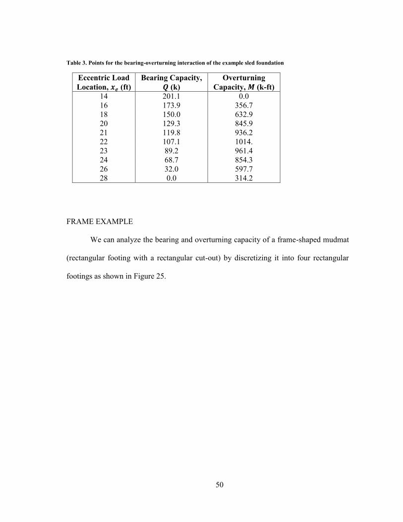
The interaction diagram for the example sled is shown in Figure 23 and the points are
listed in Table 3, along with the location of the eccentric load.Also plotted is the bearing
and overturning interaction assuming no adhesion to the base of the footing for
comparison.

49
Figure 23. Interaction diagram for example sled foundation
50
Table 3. Points for the bearing-overturning interaction of the example sled foundation
Eccentric Load
Location, (ft)
Bearing Capacity,
(k)
Overturning
Capacity, (k-ft)
14 201.1 0.0
16 173.9 356.7
18 150.0 632.9
20 129.3 845.9
21 119.8 936.2
22 107.1 1014.
23 89.2 961.4
24 68.7 854.3
26 32.0 597.7
28 0.0 314.2
FRAME EXAMPLE
We can analyze the bearing and overturning capacity of a frame-shaped mudmat
(rectangular footing with a rectangular cut-out) by discretizing it into four rectangular
footings as shown in Figure 25.

51
Figure 24. Discretized frame-shaped mudmat foundation with center cut-out
As shown in Figure 24, it is important to discretize a complex geometry in a way
that keeps continuous, rectangular bearing areas across the foundation together (Footing
1 and Footing 4). This eliminates any potential interference of the bearing failure
mechanisms that may otherwise be an artifact of the proposed analysis.

52
Assuming the foundation is installed in undrained soil with a constant undrained
shear strength profile, , we can calculate the bearing and overturning
interaction, as shown in Figure 25 (points shown in Table 4). Also plotted in this figure
is the bearing and overturning interaction assuming no adhesion of the soil to the base of
the footing.
Figure 25. Interaction diagram for frame-shaped mudmat with center cut-out

53
Table 4. Points for the interaction for frame-shaped mudmat with center cut-out
Eccentric Load
Location, (ft)
Bearing Capacity,
(k)
Overturning
Capacity, (k-ft)
10 100.8 0
12 81.27 182.9
14 64.83 322.7
15 55.76 387.8
16 46.51 406.1
17 37.67 433.6
18 24.88 445.7
19 12.00 415.9
20 0.0 392.7

54
VALIDATION THROUGH FEM
The force-moment interaction was calculated using the upper bound method of
plasticity as previously described for a 10-ft-wide by 20-ft-long mudmat foundation on
two undrained shear strength profiles:
Constant undrained shear strength,
Undrained shear strength of , at the seafloor, linearly increasing at
a rate of .
The force-moment interaction of a mudmat foundation was analyzed on two
undrained shear strength profiles using ABAQUS. This was done by evaluating the soil
response to pure bearing displacement, pure overturning rotation, and a combination of
displacements and rotations to generate an interaction diagram.
FINITE ELEMENT METHODS
The finite element method is a numerical way of solving for the stresses and
deformations in a body by breaking that body into much smaller sub-regions (identified
by nodes) that compose a mesh.
Finite element methods are used for analyzing complex geotechnical engineering
problems. Several popular programs exist for finite element analysis of foundations,
including ABAQUS and PLAXIS, among others. Finite element methods are described
in the following sections, and ABAQUS is addressed specifically.

55
Background
Finite element methods have been used to analyze soil-structure interaction for
many years. Many attribute the early development of FEM to the numerical analyses
done by Courant and later by Argyris, Turner, Clough, and others (Gupta and Meek,
1996). Courant modeled St Venant’s torsion of a square, hollow box using mesh
subdivisions of up to nine triangular nodes (Courant, 1942).
As the computational power of computers improved, meshes were expanded to
contain thousands of nodes. As the sub-regions in a mesh become smaller, the solutions
given by FEM approaches should converge towards the analytical solution (Gupta and
Meek, 1996).
FEM for structural analysis (in geotechnical engineering, the structure is the soil
mass) generally involve the following steps (Sture, 2004):
Establish stiffness relationships for the material (i.e. the elastic modulus and
shear strength of the soil)
Apply boundary conditions
Divide the material into sub-regions represented by nodes, and enforce
compatibility (all sub-regions are connected to form a continuous mesh)
Enforce equilibrium conditions at each node
Develop system of equations for all nodes in the mesh (called “assembling”)
Solve and system for all nodes

56
FEM has been used geotechnical engineering to predict the soil response during
staged construction, excavations, and more. In shallow foundation analysis, FEM is
used when the soil conditions and geometry becomes too complex to apply the simpler
methods previously described.
FEM software for geotechnical analysis is used commercially, with the most
popular programs being ABAQUS and PLAXIS in the offshore industry. Both of these
programs allow for 2-D and 3-D analyses.
ABAQUS
ABAQUS was originally released in 1978 and is a popular FEM program for
solving complex geotechnical engineering designs. In simple foundation design
applications, ABAQUS allows users to define and assign properties to a soil mass and
model the response to displacements and rotations.
DEFINING THE PROBLEM
ABAQUS allows the user to define the materials and boundary conditions for a
FEM analysis. When analyzing a shallow foundation in 2-D, we need to define:
The assembly of the soil mass (the location of the nodes in the mesh)
The assembly of the foundation (the width location of the foundation on the soil
mass)
The sub-regions (elements) and the nodes that compose them
The material properties for the soil (elastic modulus and plastic yield point)
The material properties for the foundation (rigid, no deformation)

57
The boundary conditions (the displacement and rotation of the foundation from
its original location)
One can model a constant undrained shear strength profile by defining the soil
mass to have the same material properties everywhere in the mesh. Alternatively, we
can model a linearly increasing undrained shear strength profile by appropriately
increasing the elastic modulus and plastic yield point with depth.
Since we are interested in the bearing and overturning capacity of a shallow
foundation, we can model a range of eccentric loads by specifying rotations and
displacements of the foundation. Ideally we want to view the interaction between an
applied overturning moment and the bearing capacity of the foundation.
The user can model pure bearing by inputting a vertical displacement large
enough to completely fail the soil and no rotation. Likewise, pure overturning is
modeled by inputting a rotation large enough to completely fail the soil with zero
average vertical displacement. These represent the maximum bearing and overturning
capacities of the foundation. Finally, we can represent the interactions between vertical
force and overturning moment by inputting combinations of vertical displacements and
rotations.
The ABAQUS model used in this thesis included:
The finite element mesh comprised 3,441 square elements with a total of
10,322 nodes (Figure 26).

58
An elastic modulus, , was used in the analyses. ABAQUS
requires uniaxial compression strength to characterize yield. Uniaxial
compression relates to undrained strength in simple shear according to the
relationship √
A Poisson’s ratio of 0.35 was assigned to the soil to approximate
undrained loading conditions.
An elastic-perfectly plastic material with a von Mises yield criterion was
assumed. Plastic deformations obey an associated flow law.
Four-node linear interpolation elements were utilized with full
integration.
Loading was applied in a displacement control mode to a maximum
vertical displacement of 1 ft for the case of pure translation and to a
maximum rotation of 0.35 radians for the case of pure rotation.
Imposed boundary constraints are shown in Figure 27.
Collapse loads were taken as the magnitude of the ultimate reaction
forces or moments associated with the imposed displacements.

59
Figure 26. Original mesh, prior to displacements and rotations
Figure 27. Original mesh, with applied boundary conditions

60
INTERPRETING THE RESULTS
An ABAQUS analysis produces several outputs, including a data file that can be
read with a word processor and an output file that must be viewed in the ABAQUS CAE
(Complete ABAQUS Environment).
The data file gives a detailed report of the analysis and reports requested
information for user-specified nodes. When analyzing the force-moment interaction of a
shallow foundation analysis, we view the vertical force and moment reaction applied to
the foundation during the corresponding displacement and rotation. In a 2-D analysis
this gives us the bearing capacity (in force per unit length) and corresponding
overturning capacity (in force times length per unit length) for the specified
displacement and rotation.
We can compute the total bearing capacity and overturning capacity by
multiplying these values by the length of the foundation. An example of the force-
moment interaction based on ABAQUS results is shown in Figure 28.

61
Figure 28. Interaction diagram for mudmat analyzed with ABAQUS
Note that the interaction diagram for the ABAQUS results does not decrease
between zero overturning capacity and the maximum moment capacity, as seen in the
interaction diagrams computed by the upper bound method. This is because ABAQUS
calculates the soil reactions for given displacements and rotations, and was used to
verify the maximum overturning and bearing capacities and their interaction from the
maximum overturning to the maximum bearing capacity.
The output file viewed in CAE allows the user to view stress fields, strain, the
final displaced mesh, and much more. Viewing these results allows us to see the failure

62
mechanism due to the applied displacements and rotations as well as the stress field
imparted onto the soil mass. The deformed mesh is shown below in Figure 29.
Figure 29. Deformed mesh for pure bearing with constant undrained strength
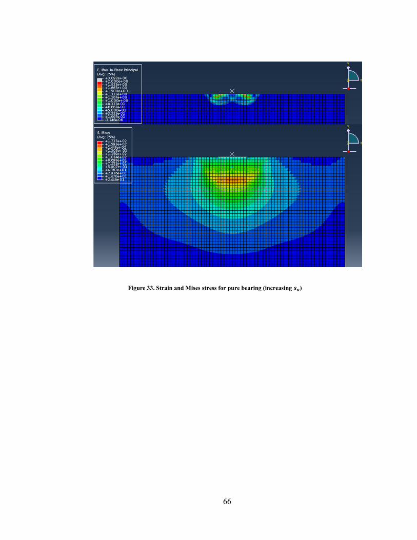
Figure 30 through Figure 35 show plots of the strain and Mises stress for pure
bearing, a combination of bearing and overturning, and pure overturning for both soil
profiles. From these plots, we can see the change in failure mechanism in the soil as a
rotation is applied to the system, as would be the case with an overturning moment.

63
Figure 30. Strain and Mises stress for pure bearing (constant )

64
Figure 31. Strain and Mises stress for combined bearing/overturning (constant )

65
Figure 32. Strain and Mises stress for pure overturning (constant )
66
Figure 33. Strain and Mises stress for pure bearing (increasing )

67
Figure 34. Strain and Mises stress for combined bearing/overturning (increasing )

68
Figure 35. Strain and Mises stress for pure overturning (increasing )

69
COMPARISON OF PROPOSED METHOD TO ABAQUS RESULTS
The results of the proposed analysis were compared to those of the ABAQUS
analysis.
COMPARISON TO RAW ABAQUS RESULTS
The results of the analyses are plotted two ways:
The magnitudes of the force-moment interaction
The magnitudes of the force-moment interaction normalized by their
corresponding maxima
Figure 36 and Figure 37 show force-moment interaction for both undrained shear
strength profiles. As evident in the plots of the magnitudes, ABAQUS predicts higher
bearing capacities and overturning capacities than the upper bound method of plasticity
for both undrained shear strength profiles.
The normalized force-moment interaction plots show the ABAQUS and upper
bound method results to closely match for the constant undrained shear strength profile.
The normalized results for the linearly increasing undrained shear strength profile show
greater normalized moment values to corresponding normalized force values.

70
Figure 36. Comparison of results for constant (raw ABAQUS results)
Figure 37. Comparison of results for linearly increasing (raw ABAQUS results)

71
COMPARISON WITH CALIBRATED ABAQUS RESULTS
The ABAQUS results were adjusted based on known bearing and overturning
capacity factors that would be expected for this type of analysis.
The bearing capacity factors were calculated from the pure bearing capacities
predicted by ABAQUS for both undrained shear strength profiles. For both profiles, the
bearing capacity factors derived from the ABAQUS results are higher than . Table
5 presents the results of this check.
The overturning capacity factors were calculated from the pure overturning
capacities predicted by ABAQUS for both undrained shear strength profiles. For both
profiles, the overturning capacity factors derived from the ABAQUS results are higher
than
. Table 5 presents the results of this check.
This check was used to calibrate the ABAQUS results by reducing the force and
moment values by the percentage indicated by the calculated factors. This reduction is
shown in Table 5 for both undrained shear strength profiles.
Table 5. Calibration reductions for ABAQUS results
Strength Profile ,
ABAQUS
Percent
Reduction
,
ABAQUS
Percent
Reduction
5.14 5.512 6.75 %
0.840 6.53 %
5.14 5.983 14.08 %
0.889 11.65 %

72
Figure 38 plots the magnitudes of the calibrated ABAQUS predictions with those
of the upper bound approach. The plots show close agreement between the upper bound
approach and the ABAQUS results for both profiles.
Figure 38. Comparison of results with calibrated ABAQUS results
Figure 39 plots the ultimate bearing capacity computed for each eccentric load
applied to the foundation as calculated by:
Upper bound plasticity analysis
Calibrated ABAQUS results

73
Figure 39. Eccentricity versus bearing capacity for UBM and ABAQUS results
It is shown in Figure 39 that for a given eccentricity, the calculated bearing
capacities are similar in magnitude for the upper bound and ABAQUS analyses.
POTENTIAL SHORTCOMINGS OF PROPOSED ANALYSIS
Careful consideration should be made when using the proposed analysis
presented in this thesis for mudmat design.
The bearing and overturning capacities calculated by this method assume that
eccentric loading acts predominately in one direction (2-D analysis). This method would
need modification to be used for mudmats with dominant eccentric loads in both planar
directions.

74
The bearing and overturning capacities calculated by the method also neglect the
effects of torsion. Significant torsion (or rotation about the vertical axis of the mudmat)
will decrease the bearing and overturning capacity of a mudmat foundation.
This analysis neglects end effects caused by the shape of the foundation and
assumes the bearing capacity factor, , is to be equal to . Thus, if the actual
shape of the mudmat foundation is closer to a rectangle or square, the bearing and
overturning capacity may be slightly underestimated. This is shown in Figure 40, where
the interaction diagram for the mudmat foundation with two footings is shown calculated
using the bearing pressure assuming a strip footing and assuming a rectangular footing
of the actual dimensions shown in Figure 6.

75
Figure 40. Interaction diagram for complex geometry with assumed end (shape) effect

76
CONCLUSIONS AND DISCUSSION
This thesis presents a simplified method for calculating the force-moment
interaction relationship of a shallow foundation subject to eccentric loading. The
method is particularly applicable to irregularly shaped foundations and composite
foundations comprising multiple pods. The solution presented here applies an upper
bound plasticity approach to the analysis of bearing and overturning capacity of shallow
foundations. Validation is provided through FEM. This method is applied to challenges
in offshore mudmat foundation design, although the principles are applicable to many
other geotechnical analyses.
Key features of the method include:
1. The foundation is subdivided into one or more sub-elements according to
the geometry of the footing. It is not necessary or desirable to subdivide a
single rectangular section into sub-divisions.
2. A rotational failure mechanism entire is presumed, with the composite
foundation assumed to act as a rigid body. The center of rotation can vary
from zero (pure rotation) to infinity (pure vertical translation). The center
of rotation is an optimization variable which will be varied to obtain a
least upper bound.

77
3. The center of rotation for each sub-element is computed from kinematic
considerations.
4. Equivalent bearing pressures acting on each component of the foundation
are computed as a function of the center of rotation for that component.
These equivalent pressures were established by matching to well-
established solutions for pure vertical translation and pure rotation of a
strip footing.
5. In cases of combined vertical-horizontal-moment (VHM) loading, a
reduction in capacity due to the horizontal load is computed assuming a
parabolic horizontal-vertical interaction function. Strictly speaking, the
analysis does not adhere to an associated flow rule, since that would
require that the work performed by the horizontal force be included in the
energy balance. Future refinements to the analysis can strictly enforce an
associated flow law.
6. Collapse load for a given center of rotation is computed by equating the
external virtual performed by the applied load to the internal virtual work
performed by the resisting soil.
7. The governing collapse load is taken as the lowest computed collapse
load computed over a range of centers of rotation from zero to infinity.
78
We can conclude that the upper bound method provides a reasonable prediction
of the bearing and overturning capacity of a mudmat foundation under eccentric loading.
This conclusion is supported by the comparison of the magnitudes of the calibrated
ABAQUS results with those from the upper bound method.
The results show that the force-moment interactions predicted by the upper
bound method match well with the calibrated ABAQUS results, although the maximum
overturning moments predicted by ABAQUS are slightly greater in magnitude. For
design purposes, the lower magnitudes calculated by the upper bound method means
more conservatism in the design than with FEM analysis.
The method presented here provides a simplified tool for routine calculations. In
its present form, it is restricted to loads that are aligned with the major axes of the
foundation. It presumes relatively simple soil strength profiles, uniform or linearly
increasing with depth. More complex situations require more rigorous analyses, such as
finite element or finite difference studies.

79
REFERENCES
American Petroleum Institute. (2010). Recommended Practice for Planning, Designing,
and Constructing Fixed Offshore Platforms. API RP 2A-WSD.
American Petroleum Institute. (2011). Geotechnical and Foundation Design
Considerations. API RP 2GEO.
Aubeny, C. P., & Murff, J. D. (2001). Lateral Undrained Resistance of Suction Caisson
Anchors. International Journal of Offshore and Polar Engineering, 11, 211-219.
Calladine, C. R. (1969). Engineering Plasticity. Oxford: Pergamon Press.
Chen, W. F., & Liu, X. L. (1991). Limit Analysis in Soil Mechanics. New York: Elsevier
Science Ltd.
Courant, R. (1942). Variational Methods for the Solution of Problems of Equilibrium
and Vibrations. Trans. American Mathematics Society, 1, 1-23.
Davis, E. H., & Booker, J. R. (1973). The Effect of Increasing Strength with Depth on
the Bearing Capacity of Clays. Geotechnique, 23, 551-563.
Drucker, D. C., & Prager, W. (1952). Soil Mechanics and Plastic Analysis for Limit
Design. Quarterly of Applied Mathematics, 7, 157-165.
Gibson, R. E., & Morgenstern, N. R. (1962). A Note on the Stability of Cuttings in
Normally Consolidated Clays. Geotechnique, 12, 212-216.

80
Gourvenec, S. (2007-1). Shape Effects on the Capacity of Rectangular Footings Under
General Loading. Geotechnique, 57, 637-646.
Gourvenec, S. (2007-2). Failure Envelopes for Offshore Shallow Foundations under
General Loadign. Geotechnique, 57, 715-728.
Gourvenec, S. (2008). Effect of Embedment on the Undrained Capacity of Shallow
Foundations under General Loading. Geotechnique, 58, 177-185.
Gourvenec, S., & Randolph, M. (2003). Effect of Strength Non-Homogeneity on the
Sahpe of Failure Envelopes for Combined Loading of Strip and Circular
Foundations on Clay. Geotechnique, 53, 575-586.
Gupta, K. K., & Meek, J. L. (1996). A Brief Histroy of the Beginning of the Finite
Element Method. International Journal for Numerical Methods in Engineering,
36, 3761-3774.
Han, S.-W. (2002). The Capacity of Suction Caissons in Isotropic and Anisotropic
Cohesive Soils Under General Loading. Doctoral Dissertation. College Station:
Texas A&M University.
Hansen, J. B. (1970). A Revised and Extended Formula for Bearing Capacity.
Copenhagen: The Danish Geotechnical Institute.
Heyman, J. (1973). Simple Plasticity Theory Applied to Soil Mechanics. Proceedings,
Symposium on the Role of Plasticity Theory in Soil Mechanics, (pp. 161-172).
Cambridge.

81
Kim, B. M. (2005). Upper Bound Analysis for Drag Anchors in Soft Clay. Doctoral
Dissertation. College Station: Texas A&M University.
Meyerhof, G. G. (1963). Some Recent Research on the Bearing Capacity of
Foundations. Canadian Geotechnical Institute.
Murff, J. D. (2008). Notes for a Technical Short Course in Plastic Limit Analysis with
Applications for Undrained Analysis of Foundations. Houston, TX.
Murff, J. D., & Aubeny, C. P. (2011). The effect of Torsion on the Sliding Resistance of
Rectangular Foundations. Proceedings, Frontiers in Offshore Geotechnics II,
(pp. 439-443). Perth, Australia.
Murff, J. D., & Hamilton, J. M. (1993). P-Ultimate for Undrained Analysis of Laterally
Loaded Piles. Journal of Geotechnical Engineering, 119, 91-107.
Murff, J. D., & Miller, T. W. (1977-1). Foundation Stability on Nonhomogeneous Clays.
Journal of the Geotechnical Engineering Division, 103, 1083-1095.
Murff, J. D., & Miller, T. W. (1977-2). Stability of Offshore Gravity Structure
Foundations Using the Upper Bound Method. Proceedings, Offshore Technology
Conference. Houston.
Murff, J. D., Wagner, D. A., & Randolph, M. F. (1989). Pipe Penetration in Cohesive
Soil. Geotechnique, 39, 213-229.

82
Randolph, M. F., & Houlsby, G. T. (1984). The Limiting Pressure on a Circular Pile
Loaded Laterally in Cohesive Soils. Geotechnique, 34, 613-623.
Randolph, M., Gaudin, C., Gourvenec, S., White, D., Boylan, N., & Cassidy, M. (2010).
Recent Advances in Offshore Geotechnics for Deep Water Oil and Gas
Developments. Ocean Engineering, 10, 818-834.
Sture, S. (2004). Finite Element Method in Geotechnical Engineering. Boulder, CO.
Vesic, A. S. (1975). Chapter 3 - Bearing Capcity of Shallow Foundations. In H. F.
Winterkorn, & H. Y. Fang, Foundation Engineering Handbook (pp. 121-147).
New York: Von Nostrand Reinhold Company.
Yun, G., & Bransby, F. (2007). The Horizontal-Moment Capacity of Embedded
Foundations in Undrained Soil. Canadian Geotechnical Journal, 44, 409-424.
Yun, G., & Bransby, F. (2007). The Undrained Vertical Bearing Capacity of Skirted
Foundations. Soils and Foundations, 47, 493-505.