Updated Ozone CART Analysis, 2000-2014

AQAST MeetingSt. Louis, MO

June 3-4, 2015

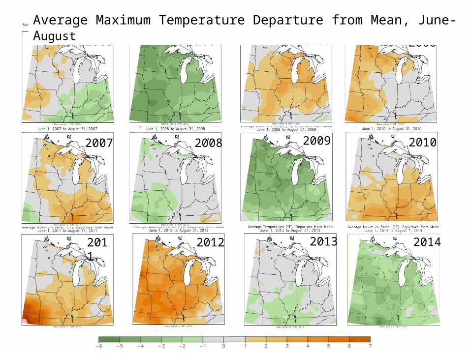
Unadjusted ozone trends

Fourth-High Values 3-year Design Values

2003 2004 2005 2006

2007 2008 2010

2011

2012

2009

Average Maximum Temperature Departure from Mean, June-August

2013 2014

Ozone CART Model

• Incorporates 30+ meteorological variables• CART is used to categorize each day by ozone

concentration and associated met conditions• Results in a decision tree with 10-15 branches, each

describing the meteorological conditions associated with a particular ozone concentration

• Trends are then developed for meteorologically similar days to minimize the effects of meteorological variability on ozone trends

What is CART analysis? – a quick review

• Classification and Regression Tree, aka binary recursive partitioning, decision tree

• Classifies data by yes/no questions -- is temp. < 75, is RH < 80; easy to interpret

• Nonparametric, so insensitive to distributions of variables

• Insensitive to transformations of variables• Insensitive to outliers and missing data• Frequently more accurate than parametric models

MEAN_W_WN <= -0.00

TerminalNode 1

STD = 0.011Avg = 0.034W = 4561.00

N = 4561

MEAN_W_WN > -0.00

TerminalNode 2

STD = 0.011Avg = 0.027W = 3887.00

N = 3887

MAXTEMP <= 69.40

Node 3MEAN_W_WN <= -0.00

STD = 0.011Avg = 0.031

W = 8448

MAXTEMP > 69.40

TerminalNode 3

STD = 0.011Avg = 0.038W = 5873.00

N = 5873

MAXTEMP <= 77.80

Node 2MAXTEMP <= 69.40

STD = 0.012Avg = 0.034W = 14321

MAXTEMP <= 85.50

TerminalNode 4

STD = 0.011Avg = 0.047W = 6839.00

N = 6839

WS3DAY <= 6.38

TerminalNode 5

STD = 0.015Avg = 0.067W = 924.00

N = 924

WS3DAY > 6.38

TerminalNode 6

STD = 0.013Avg = 0.055W = 2806.00

N = 2806

MAXTEMP > 85.50

Node 5WS3DAY <= 6.38

STD = 0.014Avg = 0.058W = 3730

MAXTEMP > 77.80

Node 4MAXTEMP <= 85.50

STD = 0.014Avg = 0.051W = 10569

Node 1MAXTEMP <= 77.80

STD = 0.015Avg = 0.041W = 24890

Sample Tree

Nodes define a set of days with similar meteorological conditions; looking at trends by node eliminates the effect of changes in meteorology on concentration trends

Meteorological variables• These variables were selected from previous model runs that had many

more variables included; these are just those that had any influence in previous models:– Daily precipitation– Cloud cover– 850 and 700 mb temperatures at 6 am – Maximum daily temperature, dew point, relative humidity, pressure– Average daily wind speed– Average daily, morning, and afternoon wind direction as N/S and E/W vectors– Morning, afternoon and evening dewpoint and pressure– Day of week– Previous day’s average temperature, pressure, wind speed, wind direction– Change in temperature and pressure from previous day– 2- and 3-day average wind speed and temperature

• Met data comes from National Weather Service data collected at airports; processing done by LADCO, with thanks to EPA and STI

Example Trend Plot – East St. Louis sites

Portion of East St. Louis CART Tree

20

40

60

80

100

OZ

PP

B

Terminal Nodes Sorted By Target Variable Prediction

Distribution of ozone among nodes

0.00

0.02

0.04

0.06

0.08

0.10

MA

XC

ON

Terminal Nodes Sorted By Target Variable Prediction

0.02

0.04

0.06

0.08

MA

XC

ON

Terminal Nodes Sorted By Target Variable Prediction

Example Model Performance

Full data set, 2000-2014

How well does2014 data fit the 00-13 model?Lower concentrationsin all nodes, but general trend is similar. Performanceis poorer for low-concentration days.

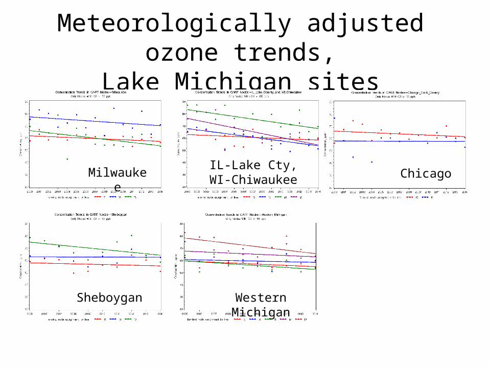
Meteorologically adjusted ozone trends,Lake Michigan sites

Chicago

Cleveland

Cincinnati

IL-Lake Cty, WI-Chiwaukee

Sheboygan

Milwaukee

Western Michigan

Chicago

Meteorologically adjusted ozone trends

Cleveland Detroit East St Louis

Cincinnati Indianapolis

Findings

• Significant predictors are daily maximum surface temperature, temperature aloft, 2- and 3-day temperature, relative humidity, and 2- and 3-day wind speeds, transport distance

• 2014 data fit well into the 2000-2013 model, especially the high-concentration days

• Trends are slightly to moderately downward in the high concentration nodes (those with average 8-hr concentrations greater than 0.055 ppm)

• Trends are consistent in all 10 areas examined

Meteorological Dataset

• Hourly surface observations from 693 sites around the US collected from National Climatic Data Center’s Integrated Surface Database (mostly airports)

• Upper air observations from 85 sites collected from NCDC’s Integrated Global Radiosonde Archive

• Each surface site is paired with closest upper air site (upper air data can be less spatially representative than surface obs)

• Hysplit back trajectories calculated for each site at noon every day to provide transport distance and u,v,w vectors

Meteorological Dataset (cont’d)

• Data for each year/site is acquired from NCDC, processed to calculated derived values (daily max/min, mixing heights, e.g.)

• QA flags assigned based on completeness, upper air site proximity.

• Lags and deviation from long term means are calculated

• Data are combined and formatted into ASCII and SAS datasets

• Available on request from LADCO