Quantifying and Communicating Uncertainty in Human PK and Dose Prediction

Douglas FergusonMay 2017

Introduction

2

• In drug discovery, prospective prediction of human pharmacokinetics facilitates the differentiation of possible clinical candidates and is a key step in the prediction of efficacious clinical dose, optimal dosing regimen and therapeutic index.

• Of similar importance to the prediction of point estimates for each human PK parameter, is the accurate quantitation and communication of the uncertainty in the point estimates.

• This presentation describes a ‘Monte-Carlo’ based approach to estimating prediction intervals for both primary PK parameters (such as Cl and Vss) and key secondary parameters such as Cmax, half-life & clinical dose.

Presentation Overview

3

• Introduction to sources of uncertainty (as applied to prediction of human PK and ‘efficacious’ clinical dose)

• Overview of reference datasets and process used to characterize the uncertainty associated with our standard PK parameter prediction tools/approaches

• ‘Monte-Carlo’ process used to combine the uncertainty in the individual predicted PK parameters to compute uncertainty in dose

• Example: drug discovery project used to illustrate the process of quantifying and communicating the uncertainty in PK and dose prediction

4

..I hate all this uncertainty!

5

Key sources of uncertainty in PK & dose prediction.

• Model uncertainty reflects the predictive accuracy of a particular model.

• Parameter uncertainty reflects uncertainty in the ‘true’ values of the mathematical model input parameters.

• Translation uncertainty reflects uncertainty in the translation from animal to man, or from one patient group to another.

• Scenario uncertainty may reflects uncertainty in how the compound is to be administered or the efficacious target exposure.

• Population uncertainty reflects uncertainty around the target population or the prevalence of a particular mutation.

Parameter

Model

Scenario

Population

Translation

The challenge is to recognise, quantify and communicate the implications of these sources of uncertainty in predictions

Examples of PK parameter prediction models - Clearance

This method predicts clearance from the equation below:

Human Cl = 33.35*(/ Rfup)0.77

(Where Rfup is the ratio of fup in rat to fup in man.)

fup Corrected intercept method (FCIM)

0

0.5

1

1.5

2

2.5

-1 -0.5 0 0.5 1 1.5

Log(

Cl)

Log(body weight)

Starts with a simple allometricplot….

Cl = *BodyWeightbRat

CynoDog

Log()

Hepatocyte Clint based IVIVe

Clint estimates from human hepatocyte incubations are scaled to a liver (metabolic) Clint according to:

Scaled liver Clint = Clint,hep *SF*fublood/fuinc

Where SF represents the product of hepatocellularity (106

cells/gliver) and liver weight (gliver/kgbody weight).

Scaled liver Clint is then converted to a ‘Predicted hepatic metabolic Clint, in vivo’ using established regression line (to correct for the general systematic under-prediction of direct IVIVe).

Input parameters are therefore plasma Cl in preclinical species & fup in rat and man.

Input parameters are therefore human hepatocyte Clint, fup, blood:plasma ratio & fuinc

Tang H, Mayersohn M. A novel model for prediction of human drug clearance by allometric scaling. Drug Metab Dispos 2005:33: 1297-1303Sohlenius-Sternbeck, A; Jones, C; Ferguson, D; Middleton, BJ; Projean, D; Floby, E;

Bylund, J; Afzelius, A. Practical use of the regression offset approach for the prediction of in-vivo intrinsic clearance from hepatocytes. Xenobiotica 42(9): 841-843 (2012)

Example of PK parameter prediction models - Vss

7

‘McGinnity 2007’ Vss prediction

-1 -0.5 0 0.5 1 1.5

-1

-0.5

0

0.5

1

1.5 dog

rat

mouse

log(Vssanimal*fup,man/fup,animal + 0.1*(1-fup,man/fup,animal))

log(

Vss m

an)

Slope = 0.954Intercept = -0.0565

Assumes tissue binding (fut) is equivalent in animals and humans and that the lower limit of Vss = distribution volume of albumin = 0.1 l/kg

animalp

manp

animalss

animalp

manp

manssfu

fuV

fu

fuV

,

,

,

,

,

, 11.0

Input parameters are therefore plasma Vss in preclinical species & fup in preclinical species and man.

Small regression correction is applied to the prediction from each species and the geometric mean of the prediction from each species in obtained.

McGinnity, DF; Collington, J; Austin, RP; Riley, RJ. Evaluation of Human Pharmacokinetics, Therapeutic Dose and Exposure Predictions Using Marketed Oral Drugs. Current Drug Metabolism 8(5): 463-479 (2007)

Typical ‘Dose Nomogram’….

8

Cl (ml/min/kg) PD target

Low(83)

Mean(139)

High(245)

1.4 500 900 16002.0 700 1250 22502.6 950 1600 2900

Range of human Clearance predictions reflecting estimated uncertainty

Target exposure uncertainty: low, average and high (in this example numbers refer to AUCu/potency)

Doses necessary to achieve the target AUC based on the variability of CL and PD targets.

Color coded to reflect a specific risk. (In this case the risk shown is formulation feasibility and risk of exceeding MAD)

• Main weakness of this approach is that it doesn’t usually express the likelihood of the various scenarios described.

• Only deals with 2 dimensions of uncertainty…which may not be sufficient.

Datasets used to assess the uncertainty associated with individual PK parameter estimation methods

9

• Lombardo et al. 2013 dataset1 (~400 compounds; human, rat, dog and monkey PK; Cl, Vss, fup)– Øie-tozer Vss (rat only, dog only, rat & dog average fut)– McGinnity Vss (rat only, dog only, rat & dog geomean Vss prediction)– FCIM Cl* (rat only fixed exponent; rat and dog)

• Astrazeneca internal Vss dataset (~110 compounds; human, rat & dog Vss & fup)– McGinnity Vss (rat only, dog only, rat & dog geomean Vss prediction)

• Paine 2011 renal clearance database2 (35 compounds)– Renal Cl* correlation method (rat correlation, dog correlation)

• Astrazeneca internal Human heps & human Mics test set compounds– IVIVe derived hepatic Cl* from human heps and human Mics

2. Paine, SW et al. Prediction of human renal clearance from preclinical species for a diverse set of drugs that exhibit both active secretion and net reabsorption. Drug Metab. Dispos. 39(6):1008-13 (2011)

1. Lombardo F. et al. Comprehensive assessment of human pharmacokinetic prediction based on in vivo animal pharmacokinetic data, part 2: clearance. J. Clin. Pharmacol. 53(2):178-191 (2013)

-1.5

-1

-0.5

0

0.5

1

1.5

-1.5 -0.5 0.5 1.5

Dat

a q

uan

tile

s

Theoretical quantiles

T-dist, 5 df

0

0.1

0.2

0.3

0.4

0.5

0.6

0.7

0.8

0.9

1

-3 -1 1 3

LOG(Clint/Clint predicted) : FCIM method

Compound data from W&L

T Distribution (5 df)

Assessing uncertainty distributions...

10

• The distribution of LOG(measured parameter/predicted parameter) was used to assess the predictive accuracy for each method when applied to the relevant test set(s)

• Example shown is the result of applying the FCIM to the W&L dataset. Green triangles derived from a histogram of the data (using 0.5σ bin width). Red line is the equation for T-distribution (5 df; Std dev = 0.48)

• The uncertainty distributions for each PK prediction method are generally best described by either a Normal or T-distribution (example QQ plot shown)

• Each distribution is characterized by type (Normal or T), number of df (if required), bias & standard deviation and used as an estimate of the prediction error distribution associated with that method.

-2

-1

0

1

2

3

-2 -1 0 1 2 3

Log(

Clin

t m

eas

ure

d)

Log(Clint predicted)

Y-axis shows ‘frequency’AUC = 1

Log(Clint/Clint predicted)

Histogram of Log(Clint/Clint pred.) values

Q-Q plot

0

0.2

0.4

0.6

0.8

1

1.2

1.4

-3 -1 1 3

LOG(renal Clint/renal Clint predicted

Renal Cl data from Paine 2011

T Distribution (3 df; SD = 0.38)

Renal Cl correlation method – use of Renal ‘Clint’

11

Normally this method is based upon the assumption that renal Cl in man can be predicted from renal Cl in animals by correcting for interspecies differences in fup and KBF.

Assessing predictive accuracy in terms of Clint prevents the prediction of possible ‘true’ values of Clrenal that exceed KBF.

However, for the purposes of uncertainty assessment, it is simpler to convert to a ‘renal Clint’ [ KBF*Clrenal/(KBF-Clrenal) ].

0

0.2

0.4

0.6

0.8

1

1.2

1.4

-3 -1 1 3LOG(renal Clint/renal Clint predicted)

Renal Cl data from Paine 2011

Normal Distribution (SD=0.35)

Renal Clhuman = Renal Cldog * (fup,human/fup,dog) * (KBFhuman/KBFdog)

Dog correlation method

Rat correlation method

Underpredicted anions

Overall uncertainty in PK parameter prediction results from combination of input parameter and model uncertainty

12

• The distribution of LOG(Vss/Vss predicted) appears to vary depending upon which reference set is used. The apparent larger uncertainty with the W&L dataset probably arises from incorporation of poorly defined PK datasets and inter-lab differences in determination of fup for different species.

• Realistic assessment of the overall uncertainty associated with a particular method requires that the reference data set, used to probe the accuracy of method, is of similar ‘quality’ to that available for the test compound.

Parameter uncertainty

Model uncertainty

Overalluncertainty

Example McGinnity Vss Method

0

0.5

1

1.5

2

2.5

3

-3 -2 -1 0 1 2 3

LOG(Vss/Vss predicted) : McGinnity Vss method (rat only)

Compound data from Astrazeneca

T Distribution (SD=0.15)

Compound data from Lombardo 2013

T-Distribution (SD=0.3)

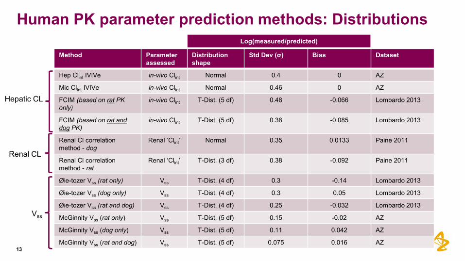
Human PK parameter prediction methods: Distributions

13

Method Parameter assessed

Distributionshape

Std Dev (σ) Bias Dataset

Hep Clint IVIVe in-vivo Clint Normal 0.4 0 AZ

Mic Clint IVIVe in-vivo Clint Normal 0.46 0 AZ

FCIM (based on rat PK only)

in-vivo Clint T-Dist. (5 df) 0.48 -0.066 Lombardo 2013

FCIM (based on rat and dog PK)

in-vivo Clint T-Dist. (5 df) 0.38 -0.085 Lombardo 2013

Renal Cl correlation method - dog

Renal ‘Clint’ Normal 0.35 0.0133 Paine 2011

Renal Cl correlation method - rat

Renal ‘Clint’ T-Dist. (3 df) 0.38 -0.092 Paine 2011

Øie-tozer Vss (rat only) Vss T-Dist. (4 df) 0.3 -0.14 Lombardo 2013

Øie-tozer Vss (dog only) Vss T-Dist. (4 df) 0.3 0.05 Lombardo 2013

Øie-tozer Vss (rat and dog) Vss T-Dist. (4 df) 0.25 -0.032 Lombardo 2013

McGinnity Vss (rat only) Vss T-Dist. (5 df) 0.15 -0.02 AZ

McGinnity Vss (dog only) Vss T-Dist. (5 df) 0.11 0.042 AZ

McGinnity Vss (rat and dog) Vss T-Dist. (5 df) 0.075 0.016 AZ

Hepatic CL

Renal CL

Vss

Log(measured/predicted)

Correlation of residual distribution with compound properties..

14

• Standard deviation of residual distribution appears to be correlated to fold-difference in free Vss between dog and rat (i.e. greater uncertainty in human Vss prediction when rat and dog free Vss don’t ‘agree’)

• May be appropriate to take these sort of observations into account when estimating the uncertainty distribution for a new compound.

-2

-1.5

-1

-0.5

0

0.5

1

1.5

2

-2 -1 0 1 2

Log(Dog free Vss/Rat free Vss)

LOG(Vss/OT Rat and Dog Pred)

LOG(Vss/OT Rat pred)

LOG(Vss/OT dog pred)

Log(

V ss

hum

an /V

sspr

ed.)

Example:

Dealing with PBPK models?

15

• More challenging to establish uncertainty distributions for PBPK models as there are multiple tissue Kp values that contribute to Vss and the overall ‘shape’ of the concentration time profile

– Requires analysis of full concentration vs time profiles in each test sets…….and how to quantify accuracy of ‘shape’ prediction?

• However, because PBPK models are based on similar assumptions (equivalent tissue binding across species) and input data as other Vss prediction methods (e.g. McGinnity & Øie-Tozer) the distribution of Log(Vss/Vss pred) should be similar

– This is supported by a PhRMA assessment that demonstrated similar predictive accuracy when comparing Arundel PBPK with other Vss prediction methods*

• Application of PBPK models requires point estimates of human tissue:bloodpartition coefficients. Simplest approach is to assume equal predictive error (log(Kp/Kppredicted) for all tissues when dealing with Vss prediction.

• Dealing with uncertainty at the Kp level (rather than Vss) prevents the generation of non-physiologically possible ‘true’ values of Vss for low Vss compounds.

Qadip

Qrapid

Clint

Arte

rial b

lood

Lung, KpLung

Adipose, KpAdip

Slow, Kpslow

Rapid, Kprapid

Liver, KpLiver

Gut, KpGut

Qgut

Qliver

Qslow

Qc

Veno

us b

lood

IV infusion

*Jones, RD et al. PhRMA CPCDC initiative on predictive models of human pharmacokinetics, part 2: Comparative assessment of prediction methods of human volume of distribution. J. Pharm. Sci. 100(10): 4074-89 (2011)

Correlation

16

• The correlation between ‘residuals’ [i.e. Log(measured/predicted)] for different methods was also assessed (for the range of PK parameter prediction models)

• In the example shown both FCIM Clint and McGinnity Vss rely upon the ratio of fup, human / fup, rat . Results is a slight correlation between method residuals.

Generally there was low correlation between the residuals for Vss and Cl prediction methods

R² = 0.154

-2

-1

0

1

2

-2 -1 0 1 2

Log(

Vss

/Vss

pre

d.)

: O

ie T

oze

r

LOG(Clint/Clint predicted) : FCIM

Lombardo data

Combining uncertainty distributions in a Monte-carloapproach...

17

• Key assumption: for a new test compound, the distribution of possible ‘true’ values (for a given human parameter) relative to the point estimate prediction, will be equivalent to the corresponding distribution of (known) true values relative to the single point ‘predictions’ for the established set of reference compounds. [Note: there will be only one actual true population mean value..]

• Step 1: Derive the point estimate prediction for each relevant PK parameter

• Step 2: Generating lists of possible ‘true’ values distrubuted around the point estimate predictions.

• Step 3: Randomly sample a single possible true value for each primary parameter (e.g. hepatic Cl, Vss, renal Cl..) from the respective distributions and then calculate/estimate a single value for each secondary parameter (such as T1/2, Cmax, Dose..) .

• Step 3 is repeated a large number of times (say 1000…) to give a distribution of possible true values for each secondary parameter of interest.

18

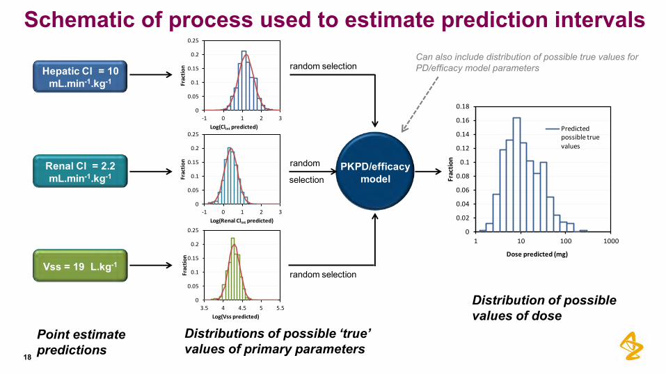
Schematic of process used to estimate prediction intervals

Point estimate predictions

Distributions of possible ‘true’ values of primary parameters

Distribution of possible values of dose

0

0.02

0.04

0.06

0.08

0.1

0.12

0.14

0.16

0.18

1 10 100 1000

Frac

tio

n

Dose predicted (mg)

Predicted possible true values

0

0.05

0.1

0.15

0.2

0.25

-1 0 1 2 3

Frac

tio

n

Log(Clint predicted)

0

0.05

0.1

0.15

0.2

0.25

3.5 4 4.5 5 5.5

Frac

tio

n

Log(Vss predicted)

0

0.05

0.1

0.15

0.2

0.25

-1 0 1 2 3

Frac

tio

n

Log(Renal Clint predicted)

PKPD/efficacy model

Hepatic Cl = 10 mL.min-1.kg-1

Renal Cl = 2.2 mL.min-1.kg-1

Vss = 19 L.kg-1

random selection

random selection

random

selection

Can also include distribution of possible true values for PD/efficacy model parameters

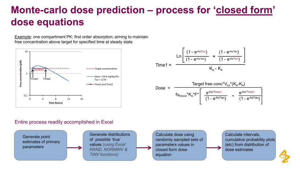
Monte-carlo dose prediction – process for ‘closed form’ dose equations

Example: one compartment PK; first order absorption; aiming to maintain free concentration above target for specified time at steady state

0.1

1

10

0 4 8 12 16

Fre

e c

on

cen

trat

ion

(µM

)

Time (hours)

Target concentration

Dose = 29.6 mg/kg PO; Tau = 12 hr

Time1 and Time2

Time1 Time2

Duration

Generate point estimates of primary parameters

Generate distributions of possible ‘true’ values (using Excel RAND, NORMINV & TINV functions)

Calculate dose using randomly sampled sets of parameters values in closed form dose equation

Calculate intervals, cumulative probability plots (etc) from distribution of dose estimates

Entire process readily accomplished in Excel

(1 - e-Ka*Dur)(1 - e-Ka*tau)

(1 - e-Ke*tau)(1 - e-Ke*Dur)*Ln

Ka - KeTime1 =

Dose = Target free conc*Vss*(Ke-Ka)

fublood*Ka*F* e-Ka*Time1

(1 - e-Ka*tau)e-Ke*Time1

(1 - e-Ke*tau)-

Monte-carlo dose prediction – process for differential equation based dose prediction

20

Use modelling software to estimate dose required to meet specified efficacy requirements for each randomly sampled set of primary parameters

or

Requires the use of model fitting software….but is the same as point estimate dose prediction (just repeated ~1000 times)

Generate point estimates of primary parameters

Generate distributions of possible ‘true’ human PK parameter values in Excel

Calculate intervals, cumulative probability plots (etc) from distribution of dose estimates

Use modelling software code to generate Normal or T-distributed sets of values (easy if NLME model enabled)

The ‘difficult’ part of the process is making qualified prior estimates of uncertainty distributions

Example: AZ Drug discovery project

21

• Oral delivery (once a day)

• Multi-exponential plasma kinetics with both hepatic and renal Cl.

• Aiming to achieve free plasma concentration that equals the free ‘IC50’ at 12 hours.

Note: this is simple example to illustrate concepts

PK parameter prediction methods employed

22

• Hepatic Clearance – estimated from Clint in hepatocytes using standard IVIVe approach. Predicted in-vivo hepatic clearance (10 ml/min/kg) was converted to in-vivo hepatic Clint by application of reverse WSM

• Renal Clearance – estimated from dog renal clearance using the ‘Dog renal Clint correlation method’. Predicted renal Cl = 2.2 ml/min/kg.

• Distribution - Arundel PBPK* approach applied using rat as primary species to derive tissue Kpvalues. Predicted Vss = 19.3 l/kg.

• fabs assumed to be 1 (based on high permeability and high fabs in all pre-clinical species)

• Ka assumed to be 3.5 hr-1 (GI prediction software)

*Arundel, PA (AstraZeneca UK). A multi-compartment model generally applicable to physiologically-based pharmacokinetics. Poster session presented at: 3rd IFAC Symposium on Modeling and Control in Biomedical Systems; 1997 March 23-26; University of Warwick

Hepatic Clint

Distributions of possible ‘true’ values for primary PK parameters..

23

• Model was written in Phoenix WinNonlin® to generate 500 sets of values for hepatic Clint, renal Clint & tissue Kps distributed around the point estimates. (Note: Vss values were then derived as a function of Kp values)

• For each parameter the generated distribution of possible ‘true’ values was assessed to ensure that it was consistent with the expected shape (based on the assumed distribution of prediction errors).

• Monte Carlo approach was used to randomly sample possible ‘true’ values from each parameter distribution - to create sets of possible primary parameter values….

Renal ClintVss

0

0.05

0.1

0.15

0.2

0.25

-1 0 1 2 3

Frac

tio

n

Log(Clint predicted)

0

0.05

0.1

0.15

0.2

0.25

3.5 4 4.5 5 5.5

Frac

tio

n

Log(Vss predicted)

0

0.05

0.1

0.15

0.2

0.25

-1 0 1 2 3

Frac

tio

n

Log(Renal Clint predicted)

Monte Carlo analysis –using Arundel PBPK model

24

Qadip

Qrapid

Clint

Arte

rial b

lood

Lung, KpLung

Adipose, KpAdip

Slow, Kpslow

Rapid, Kprapid

Liver, KpLiver

Gut, KpGut

Qgut

Qliver

Qslow

Qc

Veno

us b

lood

Oral dose

• PBPK model was written in Phoenix WinNonlin®

• Target (free) plasma concentration was set at 2 nM at 12 hours post dose on Day5. (Note: uncertainty in target concentration was not considered)

• 500 sets of possible ‘true’ PK parameter values were randomly sampled from the assumed distributions

• For each randomly sampled set of possible ‘true’ PK parameter values the oral dose was optimized such that the target free plasma concentration was attained

1

10

100

0 6 12 18 24

Fre

e p

lasm

a co

nce

ntr

atio

n (n

M)

Time (hours on Day 5)

20th percentile

80th percentile

Monte Carlo – Cumulative probability curves

25

• These plots allow the impact of uncertainty in predicted PK to be quantified in terms of ‘risk’ to the project…..

• Example – quantify the probability that the required dose will exceed the estimated maximum absorbable dose

• Example – quantify the probability that the free Cmax will exceed a threshold associated with secondary pharmacology or safety signals.

20% probability 17 hour50% probability 25 hours80% probability 35 hours

20% probability 5 mg50% probability 10 mg80% probability 27 mg

20% probability 5.1 nM50% probability 8.2 nM80% probability 13.9 nM

0

0.2

0.4

0.6

0.8

1

1 10 100 1000

Cu

mu

lati

ve P

rob

abili

ty

Human Dose (mg)

Monte Carlo dose prediction

0

0.2

0.4

0.6

0.8

1

0.001 0.01 0.1 1

Cu

mu

lati

ve P

rob

abili

ty

Free Cmax (µM)

Monte Carlo free Cmax prediction

0

0.2

0.4

0.6

0.8

1

1 10 100

Cu

mu

lati

ve P

rob

abili

ty

Terminal T1/2 (hours)

Monte Carlo T1/2 prediction

Conclusions/Comments

26

• Process described is a relatively simple approach for combining uncertainty in multiple predicted primary parameters to estimate uncertainty in key secondary parameters.

• Assessing the impact of uncertainty in PK prediction on key project ‘risks’ provides clarity for decision making.

• Work remains to be done to further refine our understanding of how certain observations impact the likely ‘uncertainty’ in PK prediction’. E.g.

– If rat & dog have the same unbound Vss how much does that reduce the uncertainty in human Vss prediction?

– To what extent does the accuracy of rat and dog Cl prediction by hepatocyte Clint IVIVe impact the uncertainty in human Cl predictions by hepatocyte Clint IVIVe?

• Need to continually track the accuracy of human PK prediction as clinical data on new candidate drugs becomes available. Ensure the predictive performance is in line with expectations.

Acknowledgements

27

• Robin McDougall• James Yates• Middleton, Brian J• Peter Webborn• Peter Gennemark

Confidentiality Notice This file is private and may contain confidential and proprietary information. If you have received this file in error, please notify us and remove it from your system and note that you must not copy, distribute or take any action in reliance on it. Any unauthorized use or disclosure of the contents of this file is not permitted and may be unlawful. AstraZeneca PLC, 1 Francis Crick Avenue, Cambridge Biomedical Campus, Cambridge, CB2 0AA, UK, T: +44(0)203 749 5000, www.astrazeneca.com

28