unstructured direct elicitation of decision rules paper...
TRANSCRIPT

Unstructured Direct Elicitation of Decision Rules
Paper 270 Min Ding John Hauser Songting Dong Daria Dzyabura Zhilin Yang Chenting Su Steven Gaskin
April 2010
A research and education initiative at the MIT Sloan School of Management
For more information,
[email protected] or 617-253-7054 please visit our website at http://digital.mit.edu
or contact the Center directly at

Unstructured Direct Elicitation of Decision Rules
Min Ding
John Hauser
Songting Dong
Daria Dzyabura
Zhilin Yang
Chenting Su
Steven Gaskin*
Forthcoming Journal of Marketing Research, 2010
* Min Ding is Smeal Research Fellow in Marketing and Associate Professor of Marketing, Smeal College of Business, Pennsylvania State University, University Park, PA 16802-3007; phone: (814) 865-0622; fax: (814) 865-3015; [email protected]. John R. Hauser is the Kirin Professor of Marketing, MIT Sloan School of Management, Massa-chusetts Institute of Technology, E40-179, One Amherst Street, Cambridge, MA 02142, (617) 253-2929, fax (617) 253-7597, [email protected]. Songting Dong is a Lecturer in Marketing, Research School of Business, the Australian National University, Canberra, ACT 0200, Australia, [email protected]. Daria Dzyabura is a doctoral student at the MIT Sloan School of Management, Massachusetts Institute of Technology, E40-170, One Amherst Street, Cambridge, MA 02142, (617) 253-2268, [email protected]. Zhilin Yang and Chenting Su are both Associate Professor of Marketing, City University of Hong Kong, Tat Chee Avenue, Kowloon, Hong Kong; phone: (852) 3442-4644; fax (852) 3442-0346; [email protected], [email protected]. Steven P. Gaskin is a Principal at Applied Marketing Science, Inc., 303 Wyman Street, Waltham, MA 02451, (781) 250-6311, [email protected]. The authors acknowledge financial support from the Research Grant Council of the Hong Kong Special Administrative Region, China (Project 9041182, CityU 1454/06H; Project 9041414, CityU 148608), Smeal Small Research Grant from Pennsylvania State University, and construc-tive comments Michael Braun, Ely Dahan, John Liechty, Young-Hoon Park, Vithala Rao, Kayande Ujwal, and from participants in a seminar given at University of Houston and a presen-tation given at the 2009 Marketing Science Conference in Ann Arbor Michigan.

Unstructured Direct Elicitation of Decision Rules
Abstract
We investigate the feasibility of unstructured direct-elicitation (UDE) of decision rules
consumers use to form consideration sets. With incentives to think hard and answer truthfully,
tested formats ask respondents to state non-compensatory, compensatory, or mixed rules for
agents who will select a product for the respondents. In a mobile-phone study two validation
tasks (one delayed 3 weeks) ask respondents to indicate which of 32 mobile phones they would
consider from a fractional 45x22 design of features and levels. UDE predicts consideration sets
better, across profiles and across respondents, than a structured direct-elicitation method (SDE).
It predicts comparably to established incentive-aligned compensatory, non-compensatory, and
mixed decompositional methods. In a more-complex (20x7x52x4x34x22) automobile study, non-
compensatory decomposition is not feasible and additive-utility decomposition is strained, but
UDE scales well. Incentives are aligned for all methods using prize indemnity insurance to
award a chance at $40,000 for an automobile plus cash. UDE predicts consideration sets better
than either additive decomposition or an established SDE method (Casemap). We discuss the
strengths and weaknesses of UDE relative to established methods.
Keywords: Decision rules, conjoint analysis, conjunctive rules, consideration sets, direct eli-
citation, incentive alignment, non-compensatory rules, product development.
1

INTRODUCTION AND PROBLEM STATEMENT
We explore direct-elicitation of decision rules that have the potential to scale to domains
that challenge decompositional approaches. These incentive-aligned approaches encourage con-
sumers to self-state both compensatory and non-compensatory rules and recognize that consum-
ers often use a consider-then-choose process, especially in complex product categories. (Our
primary focus is on the consideration decision.) We study an unstructured mechanism by which
a consumer composes an e-mail that “teaches an agent” to make decisions for the consumer.
Following current best practices we align incentives for both the consumer and the agent so that
the consumer is motivated to think hard and provide accurate answers.
Two complementary experiments compare unstructured direct elicitation (UDE) to de-
compositional and self-explication approaches that have proven successful in other empirical
comparisons. The first experiment is in a category (mobile phones, 45x22 design) in which most
decompositional approaches are feasible. The teach-an-agent task predicts consideration as well
as a standard hierarchical Bayes additive logit model and as well as established non-
compensatory decompositional decision models, but better than a pure compensatory decomposi-
tional model. We also learn that an unstructured teach-an-agent task does better than one in
which we force structure. The second experiment is in a category (automobiles, 20x7x52x4x34x22
design) in which non-compensatory decomposition is not feasible and standard decomposition
methods are challenged. UDE scales well to this application and predicts better than hierarchical
Bayes logit analysis. It also predicts better than an established structured direct-elicitation (SDE)
approach (Casemap, e.g., Srinivasan 1988). To maintain consistency all tested approaches were
incentive-aligned, even for automobiles where respondents had a reasonable chance of getting a
task-defined $40,000 automobile (plus cash if the automobile was priced less than $40,000).
2

Our research goals are “proof of concept” and “initial test.” We seek to demonstrate that
a UDE method can be designed to be incentive aligned and that, in some circumstances, UDE
will predict consideration as well or better than most commonly-used decompositional and com-
positional methods. We choose benchmarks that use a variety of methods and which have done
well in previous comparative testing.
MOTIVATION
Our research is motivated by five advances in behavioral theory and managerial practice.
First, applications such as automobiles and high-tech gadgets have become rich in features re-
quiring large numbers of profiles for even orthogonal experimental designs. For example, Dzya-
bura and Hauser (2010) describe a study used by a US auto maker that would have required a
minimal orthogonal design of 13,320 profiles. We seek methods that scale well to such complex
applications.
Second, in web-based purchasing, catalogs, and superstores consumers often select from
among 20 to 100+ products. When faced with so many alternatives, behavioral research suggests
that consumers use a two-stage consider-then-choose process rather than a one-stage compensa-
tory evaluation (e.g., Hauser and Wernerfelt 1990; Payne 1973; Roberts and Lattin 1991; Swait
and Erdem 2007). Consumers often consider only a small fraction (<10%) of the brands that are
available. We seek methods that capture the consider-then-choose decision process. (In this pa-
per, we focus primarily on the consideration stage relegating the choice stage to exploratory re-
sults in an online appendix and to future research.)
Third, particularly when faced with many feature-rich products, behavioral research and
decompositional methods suggest that some consumers use decision heuristics, such as lexico-
graphic, conjunctive, or disjunctive rules, to balance cognitive costs and decision benefits (Gil-
3
bride and Allenby 2004, 2006; Jedidi and Kohli 2005; Kohli and Jedidi 2007; Payne, Bettman
and Johnson 1988, 1993; Yee, et al. 2007). We seek methods that measure both compensatory
and non-compensatory decision rules.
Fourth, recent research suggests that incentive-alignment, through natural tasks that con-
sumers do in their daily life with real consequences, leads to greater respondent involvement,
less boredom, and higher data quality (Ding 2007; Ding, Grewal and Liechty 2005; Ding, Park
and Bradlow 2009; Kugelberg 2004; Park, Ding and Rao 2008; Prelec 2004; Smith 1976; Tou-
bia, Hauser and Garcia 2007; Toubia, et al. 2003). In theory incentive alignment gives consum-
ers sufficient motivation to describe their decision rules accurately. For a fair comparison with
established methods we accept incentive alignment as state-of-the-art and induce incentives for
the proposed methods and for established methods. We leave comparisons when incentives are
not aligned to future research.
Fifth, the diffusion of “voice-of-the-customer (VOC)” methods has created practical ex-
pertise within many market research firms in the cost-effective quantitative coding of qualitative
data (e.g., Griffin and Hauser 1993; Perreault and Leigh 1989). Although the labor cost for such
coding is linear in the number of respondents, voice-of-the-customer experience suggests that for
typical sample sizes the costs of lower-wage coders roughly balance the fixed cost of the higher-
wage analysts who are necessary for the analysis of decompositional data. (This is not surpris-
ing. Market forces have led to efficiencies so that both VOC and decomposition can compete in
the market.) Coding costs grow linearly with sample size but not with the complexity of the
product category because, empirically, consumers often strive for simplicity in their heuristic de-
cision rules (Gigerenzer and Goldstein 1996; Payne, Bettman and Johnson 1988; 1993).
4

PREVIOUS LITERATURE
Direct elicitation (sometimes called self explication or composition) has been used to
measure consumer preferences and/or attitudes for over forty years either alone or in combina-
tion with decompositional methods (Fishbein and Ajzen 1975; Green 1984; Sawtooth 1996;
Hoepfl and Huber 1975; Wilkie and Pessemier 1973). The accuracy of direct elicitation of com-
pensatory rules has varied considerably relative to decompositional methods (e.g., Akaah and
Korgaonkar 1983; Bateson, Reibstein and Boulding 1987; Green 1984; Green and Helsen 1989;
Hauser and Wisniewski 1982; Huber, et al. 1993; Leigh, MacKay and Summers 1984, Moore
and Semenik 1988; Srinivasan and Park 1997). Attempts at the structured direct elicitation of
non-compensatory rules have met with less success partly because respondents often choose pro-
files with levels they say are “unacceptable” (Green, Krieger and Banal 1988; Klein 1986; Srini-
vasan and Wyner 1988; Sawtooth 1996).
Decompositional methods have been proposed for conjunctive, disjunctive, subset con-
junctive, lexicographic, and disjunctions of conjunctions (Gilbride and Allenby 2004, 2006;
Hauser, et al. 2010; Jedidi and Kohli 2005; Kohli and Jedidi 2007; Moore and Karniouchina
2006; Yee, et al. 2007).1 Results to date suggest that non-compensatory methods predict compa-
rably to, but sometimes less well than, compensatory methods in product categories with which
respondents are familiar (batteries, computers). Non-compensatory methods are slightly better in
unfamiliar categories (smartphones, GPSs). Research suggests that approximately one-half to
two-thirds of the respondents are fit better with non-compensatory rather than compensatory me-
1 A conjunctive rule eliminates profiles with features that are not above minimum levels. A disjunctive rule accepts a profile if at least one feature is above a defined level. Subset conjunctive rules require that S features be above a minimum level. Disjunction of conjunctions rules generalize these rules further. A profile is acceptable if its features are above minimum levels on one or more defined subsets of features. Lexicographic rules order features. The fea-ture ordering implies a profile ordering based on the highest ranked feature on which the profiles vary. For consid-eration decisions, a lexicographic rule degenerates to a conjunctive model with an externally-defined cutoff.
5

thods and that the percentage is higher when respondents are asked to evaluate more profiles.
The vast majority of identified heuristics tend to be conjunctive rules (Hauser, et al. 2010). The
results are comparable whether the decision is consideration, consider-then-choose, or choice.
We are unaware of any comparisons to non-compensatory direct-elicitation methods.
THE MOBILE PHONE STUDY
It is easier to describe the direct-elicitation and decompositional tasks through examples
so we begin with a brief description of the product category that was used in the first study. In
Hong Kong, mobile phone shops line every street with “an untold selection of manufacturers and
models (German 2007).” “The entire [mobile] phone culture is far advanced” with consumers
able to buy unlocked mobile phones that can be used with any carrier (ibid.). Using local infor-
mants, observation of mobile phone stores, and discussions with potential respondents we se-
lected a set of features and feature-levels that represent the choices faced by Hong Kong respon-
dents. Pretests indicated the following feature-levels were face valid:
• Brand: Motorola, Lenovo, Nokia, Sony-Ericsson
• Color: black, blue, silver, pink
• Screen size: small (1.8 inch), large (3.0 inch)
• Thickness: slim (9 mm), normal (17 mm)
• Camera resolution: 0.5 Mp, 1.0 Mp, 2.0 Mp, 3.0 Mp
• Style: bar, flip, slide, rotational
• Base price level: $HK1080, $HK1280, $HK1480, $HK1680 [$1 ≈ $HK8]
This 4522 design is typical of compensatory decompositional analysis and at the upper
limit of non-compensatory decompositional methods which require computations that are expo-
nential in the number of feature levels.
Direct-Elicitation Tasks for the Mobile Phone Study
There were two direct-elicitation tasks in the mobile phone study. A structured direct-
6

elicitation (SDE) task asked respondents to provide rules for a friend who would act as their
agent in considering and/or purchasing a product for them. Respondents were asked to state in-
structions unambiguously and to state as many instructions as necessary. The task format had
open boxes for five rules, but respondents were not required to state five rules and they could add
rules if desired. A UDE task asked respondents to state their instructions to the agent in the form
of an e-mail to a friend. Other than a requirement to start the e-mail with “Dear friend,” respon-
dents could use any format to describe their decision rules.
Each direct-elicitation task is coded independently by two independent judges who were
blind to any hypotheses. After coding independently, the two judges meet to reconcile differenc-
es. Such coding is common in market research for both commercial use and for litigation (e.g.,
Hughes and Garrett 1990; Perreault and Leigh 1989; Wright 1973). The coding guide, the tran-
scripts, and all coded responses are available from the authors.
Explicit elimination rules are coded as such (-1 in the database) and used to eliminate
profiles in any predictions of consideration. Acceptance rules, such as “only buy Nokia,” imply
that all brands but Nokia are eliminated. Compensatory preferences are assigned an ordinal
scale. For example, if the respondent says he or she prefers Nokia, Motorola, Lenovo, and Sony-
Ericsson in that order (and does not eliminate any brand), then Nokia would be assigned a “1,”
Motorola a “2,” Lenovo a “3,” and Sony-Ericsson a “4.” In predictions these ratings are treated
as ordinal ratings. In this initial test we do not attempt to code the relative preferences among
different features. This results in weak orders of profiles (ties allowed) and is thus conservative.
We chose this conservative coding strategy so that predictions were not overly dependent on our
judges’ subjective judgments and so that their judgments would be more readily reproduced.
To illustrate the coding we provide example statements from respondents’ e-mails (re-
7

taining original language and grammar).
(Mostly non-compensatory). Dear friend, Please help me to buy a mobile phone. And there
are some requirements for you to select it for me: 1. Camera better with 3.0mp, but at least
2.0 2. Only silver or black 3. Only select Sony Ericsson or Nokia. Thank you for your help.
[Coding: -1 for 1.0 Mp, 0.5 Mp, Motorola, Lenovo, blue, and pink. 1 for 3.0 Mp.]
(Mixed non-compensatory/compensatory). Dear friend, I want to buy a mobile phone re-
cently …. The following are some requirement of my preferences. Firstly, my budget is about
$2000, the price should not more than it. The brand of mobile phone is better Nokia, Sony-
Ericsson, Motorola, because I don't like much about Lenovo. I don't like any mobile phone in
pink color. Also, the mobile phone should be large in screen size, but the thickness is not very
important for me. Also, the camera resolution is not important too, because i don't always
take photo, but it should be at least 1.0Mp. Furthermore, I prefer slide and rotational phone
design. It is hoped that you can help me to choose a mobile phone suitable for me. [Coding:
-1 for 0.5 Mp, pink, small screen, 1 for slide and rotational, and 4 for Lenovo. Our coding
is conservative. For this respondent, neither the subjective statements of relative importances
of features nor the target price were judged sufficiently unambiguous to be coded.]
(Mostly compensatory). Dear friend, I would like you to help me buy a mobile phone. Nokia
is the most favorite brand I like, but Sony Ericsson is also okay for me. Bar phones give me a
feeling of easy-to-use, so I prefer to have a new bar phone. The main features which I hope to
be included in the new mobile phone are as follows: A: 2Mp camera resolution B: Black or
Blue color C: Slimness in medium-level D: Pretty large screen Hopefully my requirements
for the purchase of this mobile phone are not too demanding, thank you for you in advance.
[Coding: 1 for Nokia, bar, 2.0 Mp, black, blue, small size, large screen, and 2 for Sony Erics-
son. The respondent’s statement ranks 2.0 Mp above 3.0 Mp, which is consistent with the
market and our design because 3.0 Mp is priced higher.]
Decompositional Task
The decompositional benchmark models were based on a three-panel format developed
by Hauser, et al. (2010). The left panel showed icons representing the 32 mobile phones. Profiles
8
were chosen from an orthogonal fractional factorial of the 4522 design. When the respondent
clicked on an icon, the mobile phone appeared in the center panel (features were described by
pictures and text). The respondent indicated whether or not he or she would consider that mobile
phone. Considered phones appeared in the right panel. The respondent could reverse the panel to
see not-considered phones and could move phones among considered, not-considered, and to-be-
evaluated until the respondent was satisfied with his/her consideration set. The data to estimate
the decompositional models are 0-vs.-1 indicators of whether each profile is included in the con-
sideration set or not.
To make the respondent’s task realistic and to avoid dominated profiles (e.g., Elrod, Lou-
viere and Davey 1992; Johnson, Meyer and Ghose 1989), the price levels for each profile were
the sum of an experimentally-varied base price level plus an increment for relevant feature-levels
(e.g., if a profile has a large screen we add $HK200 to the price). The resulting profile prices
ranged from $HK1080 to $HK2480. Prior research suggests that such Pareto designs do not af-
fect predictability substantially nor inhibit the non-compensatory use of price (Green, Helsen,
and Shandler 1988; Hauser, et. al. 2009; Toubia, et al. 2003; Toubia, et al. 2004).
Benchmark Compensatory, Non-compensatory, and Mixed Models
We chose as benchmarks commonly used compensatory and non-compensatory decom-
positional methods. Our first benchmark is the standard hierarchical Bayes logit model applied
to consideration sets using the 32 consider-vs.-not-consider observations per respondent (Hauser,
et al. 2010; Lenk, et al. 1996; Rossi and Allenby 2003, Sawtooth 2004; Swait and Erdem 2007).
The specification is an additive partworth model. Many researchers have argued that compensa-
tory models, lexicographic models, subset conjunctive, and conjunctive models can be
represented by such an additive partworth model (e.g., Jedidi and Kohli 2005; Kohli and Jedidi
9
2007; Olshavsky and Acito 1980; Yee, et al. 2007).2 Following Bröder (2000) and Yee, et al.
(2007) we also specify a q-compensatory model by constraining the additive model so that no
feature’s importance is more than q times as large as another feature’s importance. (A feature’s
importance is the difference between the maximum and minimum partworths for that feature.)
The q-compensatory model limits decision rules so that they are compensatory; the uncon-
strained additive-partworth model is consistent with both compensatory and non-compensatory
decision rules.
There are a variety of non-compensatory decompositional models/estimation methods we
can choose as benchmarks. We select two that have done well in previous research. The first is
the greedoid dynamic program which estimates a lexicographic consideration-set model (Yee, et
al. 2007). The second is logical analysis of data which estimates disjunctions of conjunctive
rules (Boros, et al. 1997). Disjunctions of conjunctive rules are generalizations of disjunctive,
conjunctive, subset conjunctive, and in the case of consideration data, lexicographic rules. Logi-
cal analysis of data has matched or outperformed other non-compensatory decompositional me-
thods, including hierarchical Bayes specifications of conjunctive, disjunctive, and subset con-
junctive models, in at least one study (Gilbride and Allenby 2004, 2006; Jedidi and Kohli 2005;
Hauser, et al. 2010). We hope that together the two methods provide reasonable initial bench-
marks to represent a broader set of non-compensatory decompositional methods. (An online ap-
pendix summarizes the benchmark methods.)
Subjects and Study Design
The subjects were students at a major university in Hong Kong who were screened to be
2Examples: If there are F feature levels and if the partworths are, in order of largest to smallest, 2F-1, 2F-2, …, 2, 1, then the additive model will act as if it were lexicographic by aspects. If S partworths have a value of β, the remain-ing partworths a value of 0, and if the utility cutoff is Sβ, then the model will act as if it were conjunctive. The ana-lytic proofs assume no measurement error.
10
18 years or older and interested in purchasing a mobile phone. After a pretest with 56 respon-
dents indicated that the questions were clear and the task not onerous, we invited subjects to
come to a computer laboratory on campus to complete the web-based survey. They also com-
pleted a delayed validation task on any internet-connected computer three weeks later. Those
who completed both tasks received $HK100 and were eligible to receive an incentive-aligned
prize (as described below). In total 143 respondents completed the entire study and provided da-
ta with which to estimate the decision rules. This represents a completion rate of 88.3%.
We focus on the consideration task rather than the choice task because (1) of growing
managerial and scientific interest in consideration decisions, (2) direct elicitation of considera-
tion rules is relatively novel in the literature, and (3) the consideration task was more likely to
provide a test of compensatory, non-compensatory, and mixed decision rules. Fortunately, initial
tests, available in an online appendix, suggest that the predictive ability for the choice task for
mobile phones (rank order within the consideration set) mimics the basic results we obtain for
the consideration task.
To obtain greater statistical power we used a within-subjects design in which subjects
complete both a direct-elicitation and a decompositional task. We use two validation tasks. One
task occurs toward the end of the web-based survey after a memory-cleansing task; the second
task is delayed by three weeks. The validation tasks use an interface identical to the decomposi-
tional task so that common-methods effects likely favor decompositional relative to direct-
elicitation. For ease of exposition, we call the first decompositional task the Calibration Task,
the first validation task the Initial Validation Task, and the second validation task the Delayed
Validation Task. Specifically, the survey proceeded as follows:
• Initial screens assured privacy and described the basic study.
• Mobile-phone features were introduced one feature at a time through text and pictures.
11
• Incentives were described for both the decompositional and direct-elicitation tasks.
• The order of the following two tasks was randomized.
• Respondents indicated which of 32 mobile phones they would consider (Calibration
Task). Considered profiles were ranked.
• Respondents described decision rules to be used by an agent to select a mobile phone
for the respondent (Structured Direct-Elicitation Task, SDE).
• “Brain-teaser” distraction questions cleared short-term memory (Frederick 2005).
• Respondents saw a new orthogonal set of 32 mobile phones (same for all respondents)
and indicated those they would consider (Initial Validation Task). Profiles were ranked.
• Respondents were asked to write an e-mail as an alternative way to instruct an agent to
select a mobile phone (E-mail-based Unstructured Direct-Elicitation Task, UDE).
• Short questions measured respondents’ comprehension of the incentives and tasks.
• (Three weeks later). Respondents saw a third orthogonal set of 32 mobile phones (same
for all respondents) and indicated those they would consider (Delayed Validation Task).
Profiles were ranked.
Caveats. This design focuses on methods comparison. At minimum, we believe the
study design has internal validity. We chose features to represent the Hong Kong market and we
chose the consideration task to represent the typical Hong Kong store. However, the most diffi-
cult induction for consideration decisions is the cognitive evaluation cost. If the evaluation cost
in the survey varies from the market, the consideration-set size in a real store might differ from
the consideration-set size in a survey. Nonetheless, the evaluation cost is constant between me-
thods because the comparison between decompositional and direct-elicitation methods is based
on the same validation data (initial and delayed). We hope that the incentives also enhance ex-
ternal validity. At minimum, pretest comments and post-survey debriefs suggest respondents be-
lieved they would behave in the market as they did in the survey. (Respondents who received
mobile phones as part of the incentives were satisfied with the mobile phones that were chosen
for them.)
12
A second concern is that either the decompositional estimation task or the direct-
elicitation task trains respondents, perhaps affecting how respondents construct decision rules
(e.g., Payne, Bettman and Johnson 1993). This would enhance internal consistency. The de-
layed task is one attempt to minimize that effect. However, internal consistency would enhance
both decompositional and direct-elicitation methods, perhaps favoring decomposition more be-
cause we use the same type of task for validation.
A third concern is an order effect for the UDE task (the e-mail task) which occurs after
the initial validation task. Potential order effects are, potentially, mitigated for the delayed vali-
dation task, but this caveat remains for the mobile phone study. Our second study randomizes
the order of the tasks and provides insight on the value of training effects (order effects).
Incentives
Designing aligned incentives for the consideration task is challenging because considera-
tion is an intermediate stage in the decision process. Other researchers have used purposefully
vague statements that were pretested to encourage respondents to trust that agents would act in
the respondents’ best interests (e.g., Kugelberg 2000). For example, if we told respondents they
would get every mobile phone considered, the best response is a large consideration set. If we
told respondents they would receive their most-preferred mobile phone, the best response is a
consideration set of exactly one mobile phone. Instead, based on pretests, we chose the follow-
ing two-stage mechanism. Because this mechanism is an heuristic, we call it “incentive aligned”
rather than the more-formal term, “incentive compatible.” Our goals with incentive alignment
are: (1) the respondents believe it is in their interests to think hard and tell the truth, (2) it is, as
much as feasible, in their interests to do so, and (3) there is no way, that is obvious to the respon-
dents, by which they improve their welfare by “cheating.”
13
Specifically, respondents were told they had a 1-in-30 chance of receiving a mobile
phone plus cash representing the difference between the price of the phone and $HK2500.3 Be-
cause we wanted both the direct-elicitation and decompositional tasks to be incentive-aligned,
respondents were told that one of the tasks would be selected by “coin flips” to determine their
prize. In addition, respondents were reminded: “It is in your best interest to think carefully when
you respond to these tasks. Otherwise you might end up with something you prefer less, should
you be selected as the winner.”
For the decompositional task respondents were told we would first randomly select one
of the three tasks (2 in the main study and 1 in the delayed study), and then select a random sub-
set of the 32 phones in that task. Respondents’ consideration decisions in the chosen task would
determine which phone they received. If there was more than one phone that matched their con-
sideration set, the rank data would distinguish the phones. The unknown random subset is impor-
tant here. This design reflects a real life scenario where a consumer constructs his/her considera-
tion set knowing that random events, such as decreased product availability, will occur prior to
purchase. If respondents “consider” too many or too few profiles they may not receive an ac-
ceptable mobile phone should they win the lottery. The incentives are aligned for both consider-
ation (our focus) and choice within the consideration set (online appendix).
For the direct-elicitation tasks respondents were told that two agents would use the res-
pondents’ decision rules to select a phone from a secret list of mobile phones. If the two agents
disagreed, a third agent would settle the disagreement. To encourage respondents to trust the
agents, respondents were told the agents would be audited and not paid unless the respondents’
3 The prize of $HK2500, approximately $US300+, might induce a wealth-endowment effect making the respondent more likely to choose more features. While the wealth-endowment effect is an interesting research opportunity, a priori it should not favor decomposition over direct elicitation or vice versa. In one example with decompositional methods, Toubia, et al. (2003) endowed all respondents with $100. They report good external validity when fore-casting market shares after the product was launched to the market.
14

instructions were followed accurately (e.g., Toubia 2006).
At the conclusion of the study, five respondents were selected randomly. Each received a
specific mobile phone (and cash) based on the mechanism described above. All respondents re-
ceived the fixed participation fee (HK$100) as promised.
To examine the face validity of the incentive alignment, we asked respondents whether
they understood the tasks and understood that it was “in their best interests to tell us their true
preferences.” There were no significant differences between the two tasks. Basically, on aver-
age, respondents found the tasks and incentive alignment easy to understand. Qualitative state-
ments also suggested that respondents believed that their answers should be truthful and reflect
their true consideration decisions. (Details in an online appendix.)
Caveat. We compare direct elicitation and decomposition when both are incentive-
aligned and leave as future research comparative tests when incentives are not aligned. Interac-
tions between task and incentives would be scientifically interesting. For example, Kramer
(2007) suggests that respondents trust researchers more when the task is more transparent.
RESULTS FROM THE MOBILE PHONE STUDY
Descriptive Statistics
The average size of the consideration set was 9.3 in the (decompositional) Calibration
Task. Consideration-set sizes were comparable for the Initial Validation Task (9.4) and the De-
layed Validation Task (9.3). All are statistically equivalent, consistent with an hypothesis that
respondents thought carefully about the tasks.
Based on the judges’ classifications of directly-elicited statements, over three-fourths of
the respondents (78.3%) asked their agents to use a mixture of compensatory and non-
compensatory rules for consideration and/or choice. Most of the remainder were compensatory
(21.0%) and only one was purely non-compensatory (0.7%).
15
Predictive Performance in the Validation Tasks
Comparative statistics. Hit rate is an intuitive measure with which to compare predic-
tive ability. However, hit rate must be interpreted with caution for consideration data because
respondents consider a relatively small set of profiles. With average consideration sets around
9.3 out of 32 (29.1%), a null model that predicts that no mobile phones will be considered will
achieve a hit rate of 70.9%. Furthermore, hit rates merge false positives and false negatives. To
distinguish results from an all-reject null model, we might examine whether we predict the size
of the consideration set correctly. But an (alternative) null model of random prediction (propor-
tional to consideration-set size) gets the consideration-set size correct.
Instead we use a version of the Kullback-Leibler divergence (KL, also known as relative
entropy) which measures the expected divergence in Shannon’s information measure between
the validation data and a model’s predictions (Chaloner and Verdinelli 1995; Kullback and Leib-
ler 1951). KL divergence rewards models that predict the consideration-set size correctly and
favors a mix of false positives and false negatives that reflect true consideration sets over those
that do not. It discriminates among models even when the hit rates might otherwise be equal.
Because it is hard to interpret the units (bits) of KL divergence, we rescale the measure relative
to the KL divergence between the validation data and a random model. (On this relative measure
larger is better. A random model has a relative KL of 0% and perfect prediction has a relative
KL of 100%.) This rescaling does not affect either the relative comparisons or the results of the
statistical tests in this paper.
In an online appendix we derive a KL formula which is comparable for both 0-vs.-1 and
probabilistic predictions. The formula, which is applied to each respondent’s data, aggregates to
false positives, true positives, false negatives, and true negatives. Specifically, let V = the num-
16
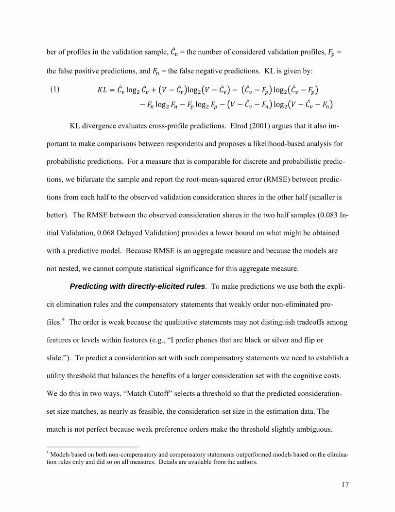
ber of profiles in the validation sample, = the number of considered validation profiles, =
the false positive e io a d pr dict ns, n = the false negative predictions. KL is given by:
log (1) log log
log log log
KL divergence evaluates cross-profile predictions. Elrod (2001) argues that it also im-
portant to make comparisons between respondents and proposes a likelihood-based analysis for
probabilistic predictions. For a measure that is comparable for discrete and probabilistic predic-
tions, we bifurcate the sample and report the root-mean-squared error (RMSE) between predic-
tions from each half to the observed validation consideration shares in the other half (smaller is
better). The RMSE between the observed consideration shares in the two half samples (0.083 In-
itial Validation, 0.068 Delayed Validation) provides a lower bound on what might be obtained
with a predictive model. Because RMSE is an aggregate measure and because the models are
not nested, we cannot compute statistical significance for this aggregate measure.
Predicting with directly-elicited rules. To make predictions we use both the expli-
cit elimination rules and the compensatory statements that weakly order non-eliminated pro-
files.4 The order is weak because the qualitative statements may not distinguish tradeoffs among
features or levels within features (e.g., “I prefer phones that are black or silver and flip or
slide.”). To predict a consideration set with such compensatory statements we need to establish a
utility threshold that balances the benefits of a larger consideration set with the cognitive costs.
We do this in two ways. “Match Cutoff” selects a threshold so that the predicted consideration-
set size matches, as nearly as feasible, the consideration-set size in the estimation data. The
match is not perfect because weak preference orders make the threshold slightly ambiguous.
4 Models based on both non-compensatory and compensatory statements outperformed models based on the elimina-tion rules only and did so on all measures. Details are available from the authors.
17
Using calibration consideration-set sizes favors neither decompositional nor direct-
elicitation methods because the threshold is also implicit in all of the decompositional estimation
methods. However, to be conservative, we also test a mixed model which estimates the consid-
eration-set-size threshold using a binary logit model with the following explanatory variables:
the stated price range, the number of non-price elimination rules, and the number of non-price
preference rules. We label this model “Estimated Cutoff.”
Because our goal is proof of concept, we feel justified in using consideration-set sizes
from the decompositional data to calibrate the binary logit model. For UDE-only applications
we suggest that the threshold model be calibrated with a pretest decompositional task or that a
more-efficient task be developed to elicit consideration-set sizes. Until such pretest tasks are
developed and tested, the reduced-data advantage of UDE for modest experimental designs is
somewhat mitigated. We return to this issue in our second study where respondents cannot eva-
luate all 25,600 orthogonal profiles severely straining additive decomposition. (Non-
compensatory decomposition is not feasible in that complex design.)
[Table 1 about here.]
Comparisons. Table 1 summarizes the predictive tests. The UDE task does significant-
ly better than the SDE task on all comparisons. It appears that the e-mail task is a more natural
task that makes it easier for respondents to articulate their decision rules.
The best decompositional method is the “HB Logit with Additive Utility.” It does sub-
stantially better on RMSE compared to other decompositional methods and better, but not signif-
icantly so, on KL. Based on the qualitative observation that most directly-elicited statements
contain both compensatory and non-compensatory instructions, it is not surprising that the mixed
(additive) decomposition model does well.
18

Comparing decompositional methods to direct-elicitation methods we see that the direct
elicitation models are best on KL, but not significantly so. The two best models on RMSE appear
to be the mixed (additive) decompositional model and the estimated-cutoff UDE model with the
former doing slightly better on the initial validation and the latter doing slightly better on the de-
layed validation. Interestingly, the RMSE for these models is only slightly larger than the lower
bound on RMSE. Decomposition and direct-elicitation are statistically (KL) and substantially
(RMSE) better than the null models. Respondents appear to use at least some non-compensatory
decision rules. Only the q-compensatory model is significantly worse on KL.
Based on Table 1 we tentatively conclude that for consideration decisions:
• the UDE task provides better data than the SDE task
• UDE predicts comparably to the best decompositional method (of those tested) on cross-profile and cross-sample validation
• in cross-sample validation the best UDE model and the best decompositional model come close to the lower bound as indicated by split-half sample agreement
• our mobile phone respondents mix elimination and compensatory decision rules.
We believe these are important findings, especially if UDE scales better than decomposi-
tion for applications with large numbers of features and feature-levels. Because incentive-
aligned direct-elicitation methods for consideration-set decisions are comparatively new relative
to incentive-aligned decomposition, we expect them to improve with further application.
Other comments. The decompositional non-compensatory models are comparable to
the additive model, superior to the q-compensatory model, and superior to analyses that use only
the directly-elicited elimination statements. (The latter are not shown in Table 1. They achieve
KL percentages of 14.9% and 14.5% for the initial and delayed validations, respectively.) This
predictive performance is consistent with results in Yee, et al. 2007.
19

ILLUSTRATIVE MANAGERIAL OUTPUTS: MOBILE PHONES
The managerial presentation of decompositional additive partworths has been developed
through decades of application. The last two columns of Table 2 provide a commonly-used for-
mat – the posterior means and standard deviations (across respondents). For example, the pink
color has, on average, a large negative partworth, but not all respondents agree: heterogeneity
among respondents is large. The “HB Logit, Additive Utility” model suggests that our respon-
dents vary considerably in their preferences for most mobile-phone features.
Academics and practitioners are still evolving the best way to summarize non-
compensatory decision rules for managerial insight. Table 2 provides one potential summary.
The third column reports the percent of respondents whose directly-elicited decision rules in-
clude a feature level as an elimination criterion. For example, 12.6% of the respondents mention
that they would eliminate any Motorola mobile phone whereas only 1.4% would eliminate any
Nokia mobile phone. The highest non-compensatory feature levels are low camera resolutions
(31.5%) and the pink color (29.4%). Price is treated slightly differently from other features in
our design because the prices that respondents saw were a combination of the base price manipu-
lation and feature-based increments. Nonetheless, 18.9% of the respondents stated they would
only accept mobile phones within specific price ranges.
[Table 2 about here.]
We attempt to summarize respondents’ directly-elicited compensatory statements in the
fourth column of Table 2 by displaying the percent of respondents who mentioned each of the
feature levels in a compensatory rule. (Respondents might mention one feature level, multiple
feature levels, or none at all.) For example, more than half (60.1%) of our respondents men-
tioned Nokia. High camera resolutions were also mentioned by large percentages of respon-
20
dents. Interesting, the percent of compensatory mentions from direct elicitation is significantly
correlated with the “HB Logit, Additive Utility” posterior mean partworths (ρ = 0.72, p < 0.001).
The posterior means of the partworths are also significantly negatively correlated with the direct-
ly-elicited feature-elimination percentages (ρ = – 0.49, p < 0.02). In our application the directly-
elicited compensatory percentages are significantly negatively correlated with directly-elicited
elimination percentages (ρ = – 0.71, p < 0.001).
We might also summarize the output of UDE by addressing a specific managerial ques-
tion. For example, if Lenovo were considering launching a $HK2500, pink, small-screen, thick,
rotational phone with a 0.5 Mp camera resolution, the majority of respondents (67.8%) would
not even consider it. On the other hand, almost everyone (all but 7.7%) would consider a Nokia,
$HK2000, silver, large-screen, slim, slide phone with 3.0 Mp camera resolution. Alternatively,
we might use respondent-level direct-elicitation data to identify market segments (an analogy to
what is now done with respondent-level partworth posterior means).
SCALABILITY: THE AUTOMOTIVE STUDY
To test scalability we select a product category and set of features that strains (or makes
infeasible) decomposition. For the non-compensatory decomposition approaches in Table 1,
running time grows exponentially with the number of feature levels (53 feature levels in autos vs.
24 in mobile phones) requiring a computational factor on the order of 500 million. An hierar-
chical Bayes additive logit model is feasible, but strained. Limits on respondent attention sug-
gest we can measure consideration for, at best, far fewer profiles than would be required by a D-
efficient orthogonal design (25,600 profiles in the automotive study). Automotive industry expe-
rience suggests that approximately 30 profiles can be evaluated in a comparative study.
The mobile-phone study suggested that a UDE task might be better than an SDE task.
21
But this may be the result of the particular structured task tested. Thus, we include an alterna-
tive, widely-applied, structured task, Casemap, that collects self-explicated data on both elimina-
tion and compensatory decision rules. Casemap has the additional advantage of not requiring the
qualitative data to be coded. We expect both the UDE e-mail task and the SDE Casemap to scale
to a realistic automotive experimental design.
We draw on an experimental design used by a major US automaker to develop strategies
to increase consideration of their vehicles (Dzyabura and Hauser 2010). We used pretests to
modify the feature levels for a student sample (vs. a national panel of auto intenders). In total
204 students at a US university completed the study. The 20x7x52x4x34x22 design was:
• Brand: Audi, BMW, Buick, Cadillac, Chevrolet, Chrysler, Dodge, Ford, Honda, Hyundai, Jeep, Kia, Lexus, Mazda, Mini, Nissan, Scion, Subaru, Toyota, Volkswagen
• Body type: compact sedan, compact SUV, crossover, hatchback, mid-size SUV, sports car, standard sedan
• EPA mileage: 15, 20, 25, 30, and 35 miles per gallon
• Glass package: none, defogger, sunroof, both
• Transmission: standard, automatic, shiftable automatic
• Trim level: base, upgrade, premium
• Quality of workmanship rating: Q3, Q4, Q5
• Crash test rating: C3, C4, C5
• Power seat: yes, no
• Engine: hybrid, internal-combustion
• Price: Profile prices, which varied from $16,000 to $40,000 were based on five manipu-lated levels plus feature-based prices.
All features were explained to respondents in opening screens using both text and pic-
tures. As training in the features, respondents evaluated a small number of warm-up profiles.
Icon/short-text descriptions of the features were used throughout the online survey and respon-
dents could return to explanation screens at any time with a single click. Pretests indicated that
22
respondents understood the feature descriptions well.
Respondent Tasks for the Automotive Study
We modified the e-mail UDE task and the three-panel decomposition task to address au-
tomobiles rather than mobile phones. For decomposition, thirty automobile profiles were chosen
randomly from the orthogonal design, eliminating unrealistic profiles such as a Mini-Cooper
SUV. (Profiles were redrawn for every respondent with a resulting D-efficiency of 0.98.) We
programmed the Casemap task to mimic as closely as possible the descriptions in Srinivasan
(1988) and Srinivasan and Wyner (1988). Respondents indicated unacceptable feature levels,
indicated their most- and least-preferred level for each feature, identified the most-important crit-
ical feature, rated the importance of every other feature relative to the critical feature, and scaled
preferences for levels within each feature. (Importance is defined as the relative value of moving
from the least-preferred level to the most-preferred level.)
After general instructions, an introduction to the features and levels, a description of the
incentives, and warm-up questions, respondents completed each of the three tasks. The order of
the tasks was randomized to mitigate the impact of order effects, if any, on relative comparisons
among methods. Screenshots are available in an online appendix. Due to the length of the au-
tomotive survey and based on the results of the mobile phone study, we did not include an initial
validation task. We relied on the delayed task. The delayed validation task used the same for-
mat as the decompositional task drawing 30 profiles per respondent randomly from a second or-
thogonal design (D-efficiency = 0.98).
All instructions, tasks, feature levels, and incentives were pretested with 34 respondents.
At the end of the pretests, respondents indicated that they understood all tasks, feature levels, and
incentives. Respondents were blind to the hypotheses of the study.
23
Incentives
With one key exception, the incentives in the automobile study were structured in the
same way as in the mobile phone study. The key exception was that it was not feasible to guar-
antee $40,000 for an automobile plus cash to one of every 30 respondents. To address this prob-
lem we bought prize indemnity insurance. For a fixed fee we were able to offer to a chosen res-
pondent a reasonable chance that he or she would get $40,000 toward an automobile (plus cash).
The features and price (≤ $40,000) would be determined by the respondent’s answers to one of
the four sections of the survey (three calibration tasks, one validation task). Specifically, respon-
dents were told that one randomly-selected respondent would draw two of twenty envelopes. If
both envelopes contained a winning card the respondent won the $40,000 prize.5 This is a stan-
dard procedure in drawings of this type. Such drawings are common for radio or automotive
promotions. Pretests indicated that these incentives were sufficient to motivate respondents to
think hard and provide truthful answers. In addition, all respondents received a fixed incentive
of $15 when they completed both the initial and the delayed questionnaires.
To examine the face validity of the incentive alignment, we asked respondents whether
they understood the tasks and understood that it was “in their best interests to tell us their true
preferences.” Although the task and the incentives were easiest to understand for Casemap (p <
0.05), they appear to be easy to understand for all three methods. We also asked the participants
whether the tasks “enable them to accurately express their preferences.” Respondents believed
the UDE and Casemap tasks enabled them to express their preferences more accurately than the
decompositional task (p < 0.01) with no significant difference between UDE and Casemap.
Generally, respondents enjoyed the three tasks, found them easy to do, put more effort into the
5 In the actual drawing the first, but not the second, envelope was a winning envelope. Because the $40,000 prize required that both envelopes be winning envelopes, the respondent received the $200 consolation prize.
24

tasks because of the incentives, and found the pictures helpful, but they did feel the tasks took a
fair amount of time. More details are available in an online appendix.
Results of the Automobile Study
Table 3 reports the rescaled KL divergence for the three rotated methods and for the null
models. RMSE relies on consideration shares among profiles in the validation data and could
not be calculated for the automotive data in which the 25,600 orthogonal profiles are spread
sparsely among the 204 respondents.
[Table 3 about here.]
Table 3 suggests that all three methods predict better than either null model. UDE pre-
dicts consideration sets better than decompositional HB-logit models reflecting the difficulty in
obtaining data for decompositional methods in complex product categories. Of the two direct-
elicitation methods, the UDE task (e-mail) appears to predict consideration better than the SDE
task (Casemap). This is consistent with the mobile phone study (unstructured structured). It is
also consistent with an hypothesis that respondents’ heuristic rules for consideration are cogni-
tively simple and that SDE encourages respondents to overstate elimination rules. For example,
Casemap-based rules miss considered profiles significantly more than UDE (p < 0.001) or de-
composition (p < 0.001).
Training Effects
In the automotive data task order was randomized. “Training” occurs if the a task fol-
lowed at least one other task. (There were no significant effects between second and third.)
UDE benefits from training, but remains best whether or not there was training. In particular:
• With training, UDE is significantly better than both Casemap and decomposition.
(p < 0.001, KL = 16.1% vs. 8.2% and 6.5%, respectively).
25

• Without training UDE is better than both Casemap and decomposition, but not signifi-
cantly so (p > 0.05, 8.4% vs. 6.8% and 6.9%, respectively).
• Training benefits UDE significantly (p < 0.002, KL = 16.1% vs. 8.4%).
• Training does not benefit either decomposition or Casemap significantly (p > 0.05, KL =
8.2% vs. 6.8% and KL = 6.5% vs. 6.8%, respectively).
Training appears to effect a significant improvement in UDE – almost doubling the KL
percentage. We see the training effect for challenging initial tasks that cause respondents to
think deeply about their decision process (Casemap or a 30-profile evaluation). This training is
substantial despite the fact that the questionnaire began with a few-profile warm-up exercise.
Perhaps future research will be able to untangle why the training effect is much stronger for UDE
than for the other methods. (A larger sample might or might not identify a significant training
effect for the other methods.)
In summary, the automotive data suggest that UDE scales to complex product categories
better than SDE or decompositional methods, that it is feasible to provide realistic incentives
even for expensive durable goods, and that there is a substantial training effect for UDE.
PROMISE AND CHALLENGES
Together the mobile-phone and automotive studies suggest that UDE holds promise for
future development. Discussions with market research managers with expertise in both quantita-
tive and qualitative methods suggest that for typical sample sizes the cost of UDE is comparable
to that for decompositional methods or structured self-explication. While UDE requires inde-
pendent coders, such coders are often billed at lower rates than experienced quantitative analysts.
Many market research firms have experienced, trained coders for qualitative data, but lack the
same depth of experience for advanced statistics (although widely-available Sawtooth Software
26
helps). If the results in this paper generalize, it appears that the choice of decomposition or UDE
for modest experimental designs should be made on grounds other than predictive ability or cost.
For complex experimental designs UDE may be more feasible than decomposition. (Of course,
for extremely large sample sizes, UDE may become too expensive.)
One concern might be that the e-mail format could prove cumbersome if there were even
more features than in the automobile study. While this is yet to be tested, behavioral theory sug-
gests that when faced with complex decisions involving many features, levels, or profiles, con-
sumers often choose cognitively-simple rules and focus on a few key features (Martignon and
Hoffrage 2002; Payne, Bettman, Johnson 1993; Shugan 1980). It is reasonable to hypothesize
that such heuristic decision processes can be captured in an e-mail/narrative format. In UDE
respondents need only describe rules for the feature levels they use to evaluate profiles. If the
decision rules are simple, the number of elicited features or feature-levels will be small.
One final advantage of UDE is the serendipitous insights that come naturally with qualit-
ative data. By comparison decompositional methods require additional qualitative questions and
the requisite coding. For example, some mobile-phone respondents gave reasons for their deci-
sion rules such as “rotational phones tend to break down” or “Lenovo has a younger image.”
Challenges
The mobile phone and automotive studies are “proof of concept,” but many challenges
remain. Among the challenges are:
1. Training. UDE benefits from training more than Casemap and decomposition even
though the validation occurred a week after the tasks. Fortunately, the automotive study
suggests that respondents can complete both a training task and a 30-profile UDE task
with reasonable incentives. More research might untangle whether respondents are learn-
27
ing the task or learning their own decision rules (Payne, Bettman and Johnson 1988;
1993). Initial results suggest that UDE applications include a substantial training task
prior to asking respondents to compose the e-mail. Casemap or 30-profile evaluation was
sufficient, but there might be other tasks that are more efficient.
2. Consideration-set size. UDE predictions benefit from a calibrated model of considera-
tion-set size. In our applications we used data from profile evaluations, but other tasks
might be more efficient. Until more efficient tasks are tested, the need for a considera-
tion-set-size model partially mitigates the value of UDE for modest-sized designs. (But
its value remains for complex designs.) Efficient tasks might serve the dual role of cali-
bration and training even if the decomposition data are not otherwise analyzed.
3. Big-ticket B2B products. We have not yet tested whether incentive alignment can be
extended to big-ticket business-to-business (B2B) products. Prize indemnity insurance
might be tried for B2B products if the firm has already solved the agency problem so that
its employees act in the best interests of the firm.
4. Incentives for consideration decisions. There are proven mechanisms for willingness
to pay such as the BDM procedure (Becker, DeGroot and Marschak 1964), but the inter-
mediate decision to consider a product is a new challenge. Even the definition of consid-
eration is an open debate (Brown and Wildt 1992). Our incentives appear to have internal
validity, motivate respondents to think hard and accurately, and are easy to understand,
but they can be improved with further experimentation and experience. We would retain
the prize, the dispute resolution among agents, and the agent-auditing process, but would
experiment with different wordings and/or award procedures.
5. Improved coding procedures. As a conservative test we sought to minimize subjectivi-
28

ty in the coding. This is both a disadvantage and a potential opportunity UDE. It is a
disadvantage because we rely on human judgment. It is a potential opportunity if more-
aggressive coding procedures can be developed to further mine the compensatory state-
ments in the qualitative data.
6. Alternative benchmarks. Although we attempted to choose a reasonably complete set
of benchmarks for the consider-vs.-not-consider task, testing versus other benchmarks
might yield further insights. We might also improve direct elicitation with adaptive self-
explication (e.g., Netzer and Srinivasan 2009). We might obtain more efficient profile
evaluations with methods based on adaptive learning and belief propagation (Dzyabura
and Hauser 2010.) HB methods might replace machine-learning non-compensatory esti-
mation.
7. Managerial summaries. There are challenges in finding efficient ways to summarize
the managerial outputs of non-compensatory decision rules, whether they be from direct
elicitation or decomposition.
Many other open questions remain such as degrees of external validity (can we predict
the share of a completely new product launched to the market), scalability (to other feature-rich
products and services), and really new product categories (where respondents may be more likely
to use non-compensatory heuristics).
29

REFERENCES
Akaah, Ishmael P. and Pradeep K. Korgaonkar (1983), “An Empirical Comparison of the Predic-
tive Validity of Self-explicated, Huber-hybrid, Traditional Conjoint, and Hybrid Conjoint
Models,” Journal of Marketing Research, 20, (May), 187-197.
Becker, Gordon M., Morris H. DeGroot, and Jacob Marschak (1964), “Measuring Utility by a
Single-Response Sequential Method,” Behavioral Science, 9 (July), 226-232.
Bateson, John E. G., David Reibstein, and William Boulding (1987), “Conjoint Analysis Relia-
bility and Validity: A Framework for Future Research,” Review of Marketing, Michael
Houston, Ed., pp. 451-481.
Boros, Endre, Peter L. Hammer, Toshihide Ibaraki, and Alexander Kogan (1997), “Logical
Analysis of Numerical Data,” Mathematical Programming, 79:163--190, August 1997
Bröder, Arndt (2000), “Assessing the Empirical Validity of the `Take the Best` Heuristic as a
Model of Human Probabilistic Inference,” Journal of Experimental Psychology: Learn-
ing, Memory, and Cognition, 26, 5, 1332-1346.
Brown, Juanita J. and Albert R. Wildt (1992), “Consideration Set Measurement,” Journal of the
Academy of Marketing Science, 20, (3), 235-263.
Chaloner, Kathryn and Isabella Verdinelli (1995), “Bayesian Experimental Design: A Review,”
Statistical Science, 10, 3, 273-304. (1995)
Ding, Min (2007), “An Incentive-Aligned Mechanism for Conjoint Analysis,” Journal of Mar-
keting Research, 54, (May), 214-223.
-----, Park, Young-Hoon, and Eric T. Bradlow (2009) “Barter Markets for Conjoint Analysis”
Management Science, 55 (6), 1003-1017.
-----, Rajdeep Grewal, and John Liechty (2005), “Incentive-Aligned Conjoint Analysis,” Journal
of Marketing Research, 42, (February), 67–82.
Dzyabura, Daria and John R. Hauser (2010), “Active Learning for Consideration Heuristics,”
Working Paper, MIT Sloan School, Cambridge MA 02139
Elrod, Terry (2001), “Recommendations for Validation of Choice Models,” 2001 Sawtooth Con-
ference Proceedings, Sequim, WA.
-----, Jordan Louviere, and Krishnakumar S. Davey (1992), “An Empirical Comparison of Rat-
ings-Based and Choice-based Conjoint Models,” Journal of Marketing Research 29, 3,
(August), 368-377.
30

Fishbein, Martin and Icek Ajzen (1975), Belief, Attitude, Intention, and Behavior, (Reading, MA:
Addison-Wesley).
Frederick, Shane (2005), “Cognitive Reflection and Decision Making.” Journal of Economic
Perspectives. 19(4). 25-42.
German, Kent (2007), “Cell phone lessons from Hong Kong,” CNET News (Crave), January 19,
http://news.cnet.com/8301-17938_105-9679298-1.html.
Gilbride, Timothy J. and Greg M. Allenby (2004), “A Choice Model with Conjunctive, Disjunc-
tive, and Compensatory Screening Rules,” Marketing Science, 23(3), 391-406.
----- and ----- (2006), “Estimating Heterogeneous EBA and Economic Screening Rule Choice
Models,” Marketing Science, 25, 5, (September-October), 494-509.
Gigerenzer, Gerd and Daniel G. Goldstein (1996), “Reasoning the Fast and Frugal Way: Models
of Bounded Rationality,” Psychological Review, 103(4), 650-669.
Green, Paul E., (1984), “Hybrid Models for Conjoint Analysis: An Expository Review,” Journal
of Marketing Research, pp. 155-169.
----- and Kristiaan Helsen (1989), “Cross-Validation Assessment of Alternatives to Individual-
Level Conjoint Analysis: A Case Study,” Journal of Marketing Research, pp. 346-350.
-----, -----, and Bruce Shandler (1988), “Conjoint Internal Validity Under Alternative Profile
Presentations,” Journal of Consumer Research, 15, (December), 392-397.
-----, Abba M. Krieger, and Pradeep Bansal (1988), “Completely Unacceptable Levels in Con-
joint Analysis: A Cautionary Note,” Journal of Marketing Research, 25, (Aug), 293-300.
Griffin, Abbie and John R. Hauser (1993), "The Voice of the Customer," Marketing Science, vol.
12, No. 1, (Winter), 1-27.
Hauser, John R. (1978), "Testing the Accuracy, Usefulness and Significance of Probabilistic
Models: An Information Theoretic Approach," Operations Research, 26, 3, (May-June),
406-421
-----, Olivier Toubia, Theodoros Evgeniou, Daria Dzyabura, and Rene Befurt (2010), “Cognitive
Simplicity and Consideration Sets,” forthcoming Journal of Marketing Research.
----- and Birger Wernerfelt (1990), “An Evaluation Cost Model of Consideration Sets,” Journal
of Consumer Research, 16 (March), 393-408.
----- and Kenneth J. Wisniewski (1982), "Dynamic Analysis of Consumer Response to Market-
ing Strategies," Management Science, 28, 5, (May), 455-486.
31

Hoepfl, Robert T. and George P. Huber (1970), “A Study of Self-Explicated Utility Models,”
Behavioral Science, 15, 408-414.
Hogarth, Robin M. and Natalia Karelaia (2005), “Simple Models for Multiattribute Choice with
Many Alternatives: When It Does and Does Not Pay to Face Trade-offs with Binary At-
tributes,” Management Science, 51, 12, (December), 1860-1872.
Huber, Joel, Dick R. Wittink, John A. Fiedler, and Richard Miller (1993), “The Effectiveness of
Alternative Preference Elicitation Procedures in Predicting Choice,” Journal of Market-
ing Research, pp. 105-114.
Hughes, Marie Adele and Dennis E. Garrett (1990), “Intercoder Reliability Estimation Ap-
proaches in Marketing: A Generalizability Theory Framework for Quantitative Data,”
Journal of Marketing Research, 27, (May), 185-195.
Jedidi, Kamel and Rajeev Kohli (2005), “Probabilistic Subset-Conjunctive Models for Heteroge-
neous Consumers,” Journal of Marketing Research, 42 (4), 483-494.
Klein, Noreen M. (1986), “Assessing Unacceptable Attribute Levels in Conjoint Analysis,” Ad-
vances in Consumer Research vol. XIV, pp. 154-158.
Kohli, Rajeev, and Kamel Jedidi (2007), “Representation and Inference of Lexicographic Prefe-
rence Models and Their Variants,” Marketing Science, 26(3), 380-399.
Kramer, Thomas (2007), “The Effect of Measurement Task Transparency on Preference Con-
struction and Evaluations of Personalized Recommendations,” Journal of Marketing Re-
search, 44, 2, (May), 224-233.
Kugelberg, Ellen (2004), “Information Scoring and Conjoint Analysis,” Department of Industrial
Economics and Management, Royal Institute of Technology, Stockholm, Sweden.
Kullback, Solomon, and Leibler, Richard A. (1951), “On Information and Sufficiency,” Annals
of Mathematical Statistics, 22, 79-86.
Leigh, Thomas W., David B. MacKay, and John O. Summers (1984), “Reliability and Validity
of Conjoint Analysis and Self-Explicated Weights: A Comparison,” Journal of Marketing
Research, pp. 456-462.
Lenk, Peter J., Wayne S. DeSarbo, Paul E. Green, Martin R. Young (1996), “Hierarchical Bayes
Conjoint Analysis: Recovery of Partworth Heterogeneity from Reduced Experimental
Designs,” Marketing Science, 15(2), p. 173--91.
Martignon, Laura and Ulrich Hoffrage (2002), “Fast, Frugal, and Fit: Simple Heuristics for
32

Paired Comparisons,” Theory and Decision, 52, 29-71.
Moore, William L. and Ekaterina Karniouchina (2006), “Screening Rules and Consumer Choice:
A Comparison of Compensatory vs. Non-Compensatory Models,” Working Paper, Uni-
versity of Utah, Salt Lake City Utah.
----- and Richard J. Semenik (1988), “Measuring Preferences with Hybrid Conjoint Analysis:
The Impact of a Different Number of Attributes in the Master Design,” Journal of Busi-
ness Research, pp. 261-274.
Netzer, Oded and V. Srinivasan (2009), “Adaptive Self-Explication of Multi-Attribute Prefe-
rences,” forthcoming Journal of Marketing Research.
Olshavsky, Richard W. and Franklin Acito (1980), “An Information Processing Probe into Con-
joint Analysis,” Decision Sciences, 11, (July), 451-470.
Park, Young-Hoon, Min Ding, Vithala R. Rao (2008) “Eliciting Preference for Complex Prod-
ucts: Web-Based Upgrading Method”, Journal of Marketing Research, 45 (5), p. 562-574
Payne, John W. (1976), “Task Complexity and Contingent Processing in Decision Making: An
Information Search,” Organizational Behavior and Human Performance, 16, 366-387.
-----, James R. Bettman and Eric J. Johnson (1988), “Adaptive Strategy Selection in Decision
Making,” Journal of Experimental Psychology: Learning, Memory, and Cognition, 14(3),
534-552.
-----, ----- and ----- (1993), The Adaptive Decision Maker, (Cambridge UK: Cambridge Universi-
ty Press).
Perreault, William D., Jr. and Laurence E. Leigh (1989), “Reliability of Nominal Data Based on
Qualitative Judgments,” Journal of Marketing Research, 26, (May), 135-148.
Prelec, Dražen (2004), “A Bayesian Truth Serum for Subjective Data,” Science, 306, (October
15), 462-466.
Roberts, John H., and James M. Lattin (1991),” Development and Testing of a Model of Consid-
eration Set Composition,” Journal of Marketing Research, 28 (November), 42940.
Rossi, Peter E., Greg M. Allenby (2003), “Bayesian Statistics and Marketing,” Marketing
Science, 22(3), p. 304-328.
Sawtooth Software, Inc. (1996), “ACA System: Adaptive Conjoint Analysis,” ACA Manual,
(Sequim, WA: Sawtooth Software, Inc.)
----- (2004), “The CBC Hierarchical Bayes Technical Paper,” (Sequim, WA: Sawtooth Soft-
33

ware, Inc.)
Shugan, Steven (1980), “The Cost of Thinking,” Journal of Consumer Research, 27(2), 99-111.
Dzyabura, Daria and John R. Hauser (2009), “Active Learning for Consideration Heuristics,”
MIT Sloan Working Paper, Cambridge, MA. October.
Smith, Vernon L. (1976), “Experimental Economics: Induced Value Theory,” American Eco-
nomic Review, 66 (May), 274-79.
Srinivasan, V. (1988), “A Conjunctive-Compensatory Approach to The Self-Explication of Mul-
tiattributed Preferences,” Decision Sciences, pp. 295-305.
----- and Chan Su Park (1997), “Surprising Robustness of the Self-Explicated Approach to Cus-
tomer Preference Structure Measurement,” Journal of Marketing Research, 34, (May),
286-291.
----- and Gordon A. Wyner (1988), “Casemap: Computer-Assisted Self-Explication of Multiat-
tributed Preferences,” in W. Henry, M. Menasco, and K. Takada, Eds, Handbook on New
Product Development and Testing, (Lexington, MA: D. C. Heath), 91-112.
Swait, Joffre and Tülin Erdem (2007), “Brand Effects on Choice and Choice Set Formation Un-
der Uncertainty,” Marketing Science 26, 5, (September-October), 679-697.
Toubia, Olivier (2006), “Idea Generation, Creativity, and Incentives,” Marketing Science, 25, 5,
(September-October), 411-425.
-----, John R. Hauser and Rosanna Garcia (2007), “Probabilistic Polyhedral Methods for Adaptive
Choice-Based Conjoint Analysis: Theory and Application,” Marketing Science, 26, 5, (Sep-
tember-October), 596-610.
-----, -----, and Duncan Simester (2004), “Polyhedral Methods for Adaptive Choice-based Conjoint
Analysis,” Journal of Marketing Research, 41, 1, (February), 116-131.
-----, Duncan I. Simester, John R. Hauser, and Ely Dahan (2003), “Fast Polyhedral Adaptive
Conjoint Estimation,” Marketing Science, 22(3), 273-303.
Wilkie, William L. and Edgar A. Pessemier (1973), “Issues in Marketing’s Use of Multi-attribute
Attitude Models,” Journal of Marketing Research, 10, (November), 428-441.
Wright, Peter (1973), “The Cognitive Processes Mediating Acceptance of Advertising,” Journal
of Marketing Research, 10, (February), 53-62.
Yee, Michael, Ely Dahan, John R. Hauser and James Orlin (2007) “Greedoid-Based Noncom-
pensatory Inference,” Marketing Science, 26, 4, (July-August), 532-549.
34

35
TABLE 1. PREDICTIVE ABILITY MOBILE PHONE STUDY
Initial Validation Delayed Validation
Relative KL Divergence1
Cross Valida-tion RMSE2
Relative KL Divergence
Cross Valida-tion RMSE
Decompositional Methods
HB Logit, Additive Utility 25.3%* 0.088 23.7%* 0.089
HB Logit, q-Compensatory 19.3% 0.144 17.6% 0.127
Greedoid Dynamic Program3 24.5%* 0.136 23.0%* 0.118
Logical Analysis of Data4 23.2%* 0.140 22.4%* 0.133
Structured Direct-Elicitation Methods (SDE)
Match Cutoff 19.5% 0.125 19.7 0.110
Estimated Cutoff 20.0% 0.118 19.2 0.110
Unstructured Direct-Elicitation Methods (UDE)
Match Cutoff 27.6%* 0.103 25.4%* 0.100
Estimated Cutoff 27.1%* 0.094 24.8%* 0.088
Null Models
Reject All 0.0% 0.370 0.0% 0.364
Random Proportional to Considera-tion Share in Calibration Data 0.0% 0.228 0.0% 0.219
Split-half Predicted vs. Observed Profile Share Cross Validation -- 0.083 -- 0.068
1Rescaled Kullback-Leibler Divergence. Larger numbers are better. 2Bi-fold cross validation compares predictions of profile shares from each half of the sample to profile shares in the remaining half. Smaller numbers are better. 3Estimates a lexicographic model. 4Estimates disjunctive, conjunctive, subset conjunctive, and/or disjunctions of conjunctions models.
* Best in column or not significantly different than best in column at the 0.05 level.

36
TABLE 2: RULES AND PARTWORTHS BY FEATURE LEVEL, MOBILE PHONES
Feature Level Direct Elicitation
Percent Elimination
Direct Elicitation Percent
Compensatory
Decomposition HB Mean
Partworths1
HB Partworth Heterogeneity
(Std Dev)2
Brand Motorola 12.6% 14.7% –– ––
Lenovo 15.4% 13.3% -0.233 0.500
Nokia 1.4% 60.1% 1.135 0.354
Sony-E 3.5% 48.3% 0.833 0.406
Color Black 2.8% 53.8% –– ––
Blue 8.4% 24.9% -0.423 0.393
Silver 0.7% 46.2% 0.068 0.751
Pink 29.4% 21.7% -2.073 2.354
Screen Size Small 16.8% 0.0% –– ––
Large 0.0% 79.0% 2.380 1.618
Thickness Slim 0.0% 51.0% –– ––
Normal 7.0% 4.9% -0.629 0.413
Resolution 0.5 Mp 31.5% 14.0% –– ––
1.0 Mp 23.8% 25.2% 1.021 0.422
2.0 Mp 3.5% 69.2% 3.348 1.738
3.0 Mp 0.0% 81.1% 3.731 2.122
Style Bar 5.6% 43.4% –– ––
Flip 8.4% 34.3% -0.127 0.411
Slide 4.9% 42.0% 0.076 0.391
Rotational 16.8% 28.7% -0.581 0.960
Price 18.9% 2.8% –– ––
Base Price $HK1080 –– –– –– ––
$HK1280 –– –– -0.095 0.136
$HK1480 –– –– -0.031 0.401
$HK1680 –– –– -0.167 0.307
1 Posterior mean of the partworths from the decompositional “HB Logit, Additive Utility” model. 2 Posterior partworth standard deviation (across respondents) from the “HB Logit, Additive Utility” model.

37
TABLE 3. PREDICTIVE ABILITY AUTOMOBILE STUDY
Delayed Validation
Relative KL Divergence1
Decompositional Methods2
HB Logit, Additive Utility 6.6%
HB Logit, q-Compensatory 3.7%
Casemap (a version of SDE)
Match Cutoff 7.8%
Estimated Cutoff3 7.4%
Unstructured Direct-Elicitation Methods (UDE)
Match Cutoff 13.6%*
Estimated Cutoff4 13.2%*
Null Models
Reject All 0.0%
Random Proportional to Consideration Share in Cali-bration Data 0.0%
1Rescaled Kullback-Leibler Divergence. Larger is better. 2Greedoid dynamic program and logical analysis of data are not feasible computationally for the automotive study. 3”Utility” cutoff determined in calibration data and then applied to validation data. 4Logit-based estimation of consideration-set size as in the mobile-phone study.
* Best in column or not significantly different than best at the 0.05 level.
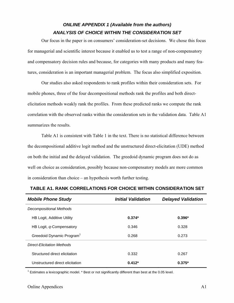
Online Appendices A1
ONLINE APPENDIX 1 (Available from the authors)
ANALYSIS OF CHOICE WITHIN THE CONSIDERATION SET Our focus in the paper is on consumers’ consideration-set decisions. We chose this focus
for managerial and scientific interest because it enabled us to test a range of non-compensatory
and compensatory decision rules and because, for categories with many products and many fea-
tures, consideration is an important managerial problem. The focus also simplified exposition.
Our studies also asked respondents to rank profiles within their consideration sets. For
mobile phones, three of the four decompositional methods rank the profiles and both direct-
elicitation methods weakly rank the profiles. From these predicted ranks we compute the rank
correlation with the observed ranks within the consideration sets in the validation data. Table A1
summarizes the results.
Table A1 is consistent with Table 1 in the text. There is no statistical difference between
the decompositional additive logit method and the unstructured direct-elicitation (UDE) method
on both the initial and the delayed validation. The greedoid dynamic program does not do as
well on choice as consideration, possibly because non-compensatory models are more common
in consideration than choice – an hypothesis worth further testing.
TABLE A1. RANK CORRELATIONS FOR CHOICE WITHIN CONSIDERATION SET
Mobile Phone Study Initial Validation Delayed Validation
Decompositional Methods
HB Logit, Additive Utility 0.374* 0.396*
HB Logit, q-Compensatory 0.346 0.328
Greedoid Dynamic Program1 0.268 0.273
Direct-Elicitation Methods
Structured direct elicitation 0.332 0.267
Unstructured direct elicitation 0.412* 0.375*
1 Estimates a lexicographic model. * Best or not significantly different than best at the 0.05 level.

Online Appendices A2
For the automotive study, UDE is best or not significantly different than best. However,
unlike for consideration decisions, UDE is not significantly better in predicting ranks within the
consideration set than the decompositional methods. We are hesitant to read too much into this
result because the variation across respondents in rank correlations is large compared to variation
across methods. The ratio of the standard deviation to the mean is between 2.0 and 2.7 for the
four methods (although the results in Table A2 are paired t-tests with greater power).
The lack of statistical power for ranks in the automotive study is explained, in part, be-
cause we focused that study on consideration-set decisions. In the current managerial climate,
understanding automotive consideration is extremely important. The large number of potential
features and levels (53) relative to the sizes of the consideration sets (~ 10 profiles) challenged
all methods. Nonetheless there remains the scientific challenge of improving and testing UDE
for automotive ranks within the consideration set. For example, more-aggressive coding might
resolve ties in weak orderings to improve the predictive ability of UDE for ranks.
An alternative hypothesis is that UDE is best for heuristic consideration decisions while
additive decomposition is best if compensatory rules are used to rank profiles within a considera-
tion set. (See also the greedoid dynamic program results in Table A1.) We cannot resolve this
hypothesis with our focused studies, but it is an interesting topic for future research.
TABLE A2. RANK CORRELATIONS FOR CHOICE WITHIN CONSIDERATION SET
Automotive Study Delayed Validation
Decompositional Methods
HB Logit, Additive Utility 0.204*
HB Logit, q-Compensatory 0.151*
Direct-Elicitation Methods
Structured direct-elicitation (Casemap) 0.108
Unstructured direct-elicitation (e-mail) 0.150*
* Best or not significantly different than best at the 0.05 level.
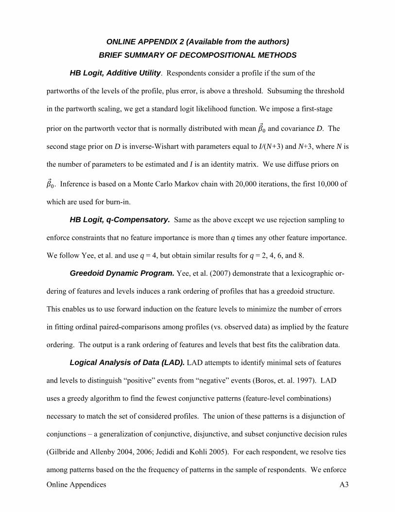
Online Appendices A3
ONLINE APPENDIX 2 (Available from the authors)
BRIEF SUMMARY OF DECOMPOSITIONAL METHODS
HB Logit, Additive Utility. Respondents consider a profile if the sum of the
partworths of the levels of the profile, plus error, is above a threshold. Subsuming the threshold
in the partworth scaling, we get a standard logit likelihood function. We impose a first-stage
prior on the partworth vector that is normally distributed with mean and covariance D. The
second stage prior on D is inverse-Wishart with parameters equal to I/(N+3) and N+3, where N is
the number of parameters to be estimated and I is an identity matrix. We use diffuse priors on
. Inference is based on a Monte Carlo Markov chain with 20,000 iterations, the first 10,000 of
which are used for burn-in.
HB Logit, q-Compensatory. Same as the above except we use rejection sampling to
enforce constraints that no feature importance is more than q times any other feature importance.
We follow Yee, et al. and use q = 4, but obtain similar results for q = 2, 4, 6, and 8.
Greedoid Dynamic Program. Yee, et al. (2007) demonstrate that a lexicographic or-
dering of features and levels induces a rank ordering of profiles that has a greedoid structure.
This enables us to use forward induction on the feature levels to minimize the number of errors
in fitting ordinal paired-comparisons among profiles (vs. observed data) as implied by the feature
ordering. The output is a rank ordering of features and levels that best fits the calibration data.
Logical Analysis of Data (LAD). LAD attempts to identify minimal sets of features
and levels to distinguish “positive” events from “negative” events (Boros, et. al. 1997). LAD
uses a greedy algorithm to find the fewest conjunctive patterns (feature-level combinations)
necessary to match the set of considered profiles. The union of these patterns is a disjunction of
conjunctions – a generalization of conjunctive, disjunctive, and subset conjunctive decision rules
(Gilbride and Allenby 2004, 2006; Jedidi and Kohli 2005). For each respondent, we resolve ties
among patterns based on the the frequency of patterns in the sample of respondents. We enforce

Online Appendices A4
cognitive simplicity by limiting the number of feature-levels in a pattern (Hauser, et al. 2010).
ONLINE APPENDIX 3 (Available from the authors)
DETAILS OF KULLBACK-LEIBLER DIVERGENCE FOR OUR DATA
The Kullback-Leibler divergence (KL) is an information-theory-based measure of the di-
vergence from one probability distribution to another. Because it is calculated for each respon-
dent, we suppress the respondent subscript. We seek the divergence from the predicted consid-
eration probabilities to those that are observed in the validation data , recognizing the discrete na-
ture of the data ( such that 1 if the respondent considers profile k, 0 otherwise). We pre-
dict whether the respondent considers profile k. Call this prediction . Let be the vector of
the ’s. If the ’s were always probabilities (and the number of profiles is not too large), the
divergence from the data ( ) to the model being tested ( ) ould be: w
|| log(A1) 1 log11
Equation A1 is poorly defined for discrete predictions ( = 0 or 1) and very sensitive to
false predictions when approaches 0 or 1. For a fair comparison of both discrete and probabil-
istic predictions we focus on false positives, true positives, false negatives, and true negatives to
separate the summation into four components.1 Let V = the number of profiles in the validation
sample, = the number of considered validation profiles, = the false positive predictions,
and = the false negative predictions. Then the KL divergence is given by the following equa-
tion where Sc,c is the set of profiles that are considered in the calibration data and considered in
the validation data. The sets Sc,nc, Snc,c, and S c are defined sim nc → not considered). nc,n ilarly (
log log log log,,,,
1 As per information theory, some information is lost in aggregation. If future researchers develop UDE methods that produce probabilistic predictions, and if the number of profiles is not too large, then comparisons might be made with Equation 1. When comparing discrete and probabilistic predictions we chose to use Equation A2.
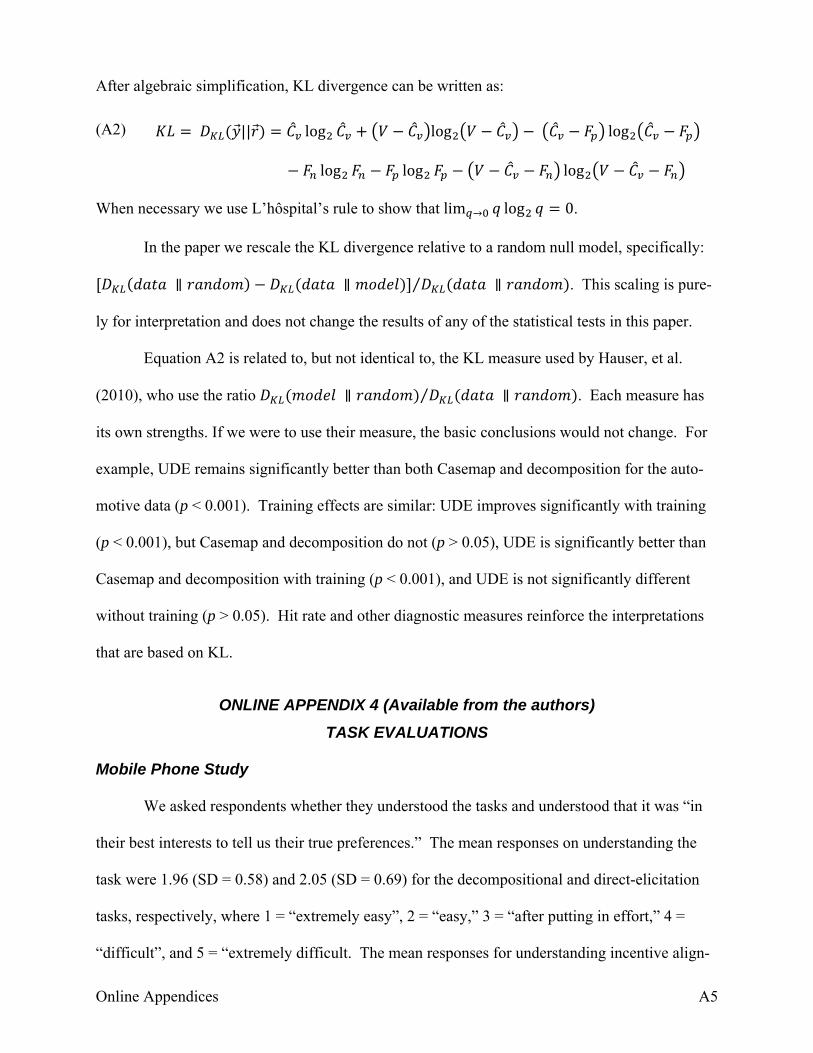
Online Appendices A5
After algebraic simplification, KL divergence can be written as :
||(A2) log log og
log log
l
log
When necessary we use L’hôspital’s rule to show that lim log 0.
In the paper we rescale the KL divergence relative to a random null model, specifically:
⁄ . This scaling is pure-
ly for interpretation and does not change the results of any of the statistical tests in this paper.
Equation A2 is related to, but not identical to, the KL measure used by Hauser, et al.
(2010), who use the ratio ⁄ . Each measure has
its own strengths. If we were to use their measure, the basic conclusions would not change. For
example, UDE remains significantly better than both Casemap and decomposition for the auto-
motive data (p < 0.001). Training effects are similar: UDE improves significantly with training
(p < 0.001), but Casemap and decomposition do not (p > 0.05), UDE is significantly better than
Casemap and decomposition with training (p < 0.001), and UDE is not significantly different
without training (p > 0.05). Hit rate and other diagnostic measures reinforce the interpretations
that are based on KL.
ONLINE APPENDIX 4 (Available from the authors)
TASK EVALUATIONS
Mobile Phone Study
We asked respondents whether they understood the tasks and understood that it was “in
their best interests to tell us their true preferences.” The mean responses on understanding the
task were 1.96 (SD = 0.58) and 2.05 (SD = 0.69) for the decompositional and direct-elicitation
tasks, respectively, where 1 = “extremely easy”, 2 = “easy,” 3 = “after putting in effort,” 4 =
“difficult”, and 5 = “extremely difficult. The mean responses for understanding incentive align-
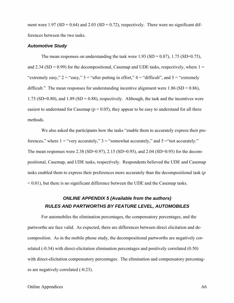
Online Appendices A6
ment were 1.97 (SD = 0.64) and 2.03 (SD = 0.72), respectively. There were no significant dif-
ferences between the two tasks.
Automotive Study
The mean responses on understanding the task were 1.93 (SD = 0.87), 1.75 (SD=0.75),
and 2.34 (SD = 0.99) for the decompositional, Casemap and UDE tasks, respectively, where 1 =
“extremely easy,” 2 = “easy,” 3 = “after putting in effort,” 4 = “difficult”, and 5 = “extremely
difficult.” The mean responses for understanding incentive alignment were 1.86 (SD = 0.86),
1.73 (SD=0.80), and 1.89 (SD = 0.88), respectively. Although, the task and the incentives were
easiest to understand for Casemap (p < 0.05), they appear to be easy to understand for all three
methods.
We also asked the participants how the tasks “enable them to accurately express their pre-
ferences,” where 1 = “very accurately,” 3 = “somewhat accurately,” and 5 =“not accurately.”
The mean responses were 2.38 (SD=0.97), 2.15 (SD=0.95), and 2.04 (SD=0.95) for the decom-
positional, Casemap, and UDE tasks, respectively. Respondents believed the UDE and Casemap
tasks enabled them to express their preferences more accurately than the decompositional task (p
< 0.01), but there is no significant difference between the UDE and the Casemap tasks.
ONLINE APPENDIX 5 (Available from the authors)
RULES AND PARTWORTHS BY FEATURE LEVEL, AUTOMOBILES
For automobiles the elimination percentages, the compensatory percentages, and the
partworths are face valid. As expected, there are differences between direct elicitation and de-
composition. As in the mobile phone study, the decompositional partworths are negatively cor-
related (-0.34) with direct-elicitation elimination percentages and positively correlated (0.50)
with direct-elicitation compensatory percentages. The elimination and compensatory percentag-
es are negatively correlated (-0.23).

Online Appendices A7
ONLINE APPENDIX 6 (Available from the authors)
SCREENSHOTS OF THE STUDIES
Screenshots from both studies will be made available in an online appendix. They are not
included in this document because they would cause the document to be an extremely large file
challenging electronic transmission, storage, and printing.