unsteady aerodynamic and dynamic analysis of the meridian
TRANSCRIPT
Unsteady Aerodynamic and Dynamic Analysis of the
Meridian UAS in a Rolling-Yawing Motion
By
Ryan Lykins
Submitted to the graduate degree program in Aerospace Engineering and the Graduate Faculty of
the University of Kansas in partial fulfillment of the requirements for the degree of Master of
Science.
________________________________
Chairperson, Dr. Shawn S. Keshmiri
________________________________
Dr. C. Edward Lan
________________________________
Dr. Richard Hale
Date Defended: November 27th
, 2013

ii
The Thesis Committee for Ryan Lykins
certifies that this is the approved version of the following thesis:
Unsteady Aerodynamic and Dynamic Analysis of the
Meridian UAS in a Rolling-Yawing Motion
________________________________
Chairperson, Dr. Shawn S. Keshmiri
Date approved: November 27th
, 2013
iii
Abstract
The nonlinear and unsteady aerodynamic effects of operating the Meridian unmanned
aerial system (UAS) in crosswinds and at high angular rates is investigated in this work. The
Meridian UAS is a large autonomous aircraft, with a V-tail configuration, operated in Polar
Regions for the purpose of remotely measuring ice sheet thickness. The inherent nonlinear
coupling produced by the V-tail, along with the strong atmospheric disturbances, has made
classical model identification methods inadequate for proper model development. As such, a
powerful tool known as Fuzzy Logic Modeling (FLM) was implemented to generate time-
dependent, nonlinear, and unsteady aerodynamic models using flight test data collected in
Greenland in 2011.
Prior to performing FLM, compatibility analysis is performed on the data, for the purpose
of systematic bias removal and airflow angle estimation. As one of the advantages of FLM is the
ability to model unsteady aerodynamics, the reduced frequency for both longitudinal and lateral-
directional motions is determined from the unbiased data, using Theodorsen’s theory of
unsteadiness, which serves as an input parameter in modeling. These models have been used in
this work to identify pilot induced oscillations, unsteady coupling motions, unsteady motion due
to the slipstream and cross wind interaction, and destabilizing motions and orientations. This
work also assesses the accuracy of preliminary aircraft dynamic models developed using
engineering level software, and addresses the autopilot Extended Kalman Filter state estimations.

iv
Acknowledgements
Firstly I would like thank Dr. Shawn S. Keshmiri for his continuing support, friendship,
and mentorship over the past four and a half years. Without his genuine care, depth of
knowledge, strong worth ethic and passion to continuously learn I would not have acquired the
skills I have developed nor accomplished as much as I have. I will never forget this time, and I
hope we have the chance to work together again in the future.
This work would not have been possible without Dr. C. Edward Lan, as he developed the
Fuzzy Logic Modeling methods and software used in this research. I would like to thank Dr.
Lan for making the trip to Kansas in 2011 as I began my research to instruct me on using his
software, as well as continually and patiently responding to the numerous questions I have had
over the past two years.
Without Dr. Hale I would not have had the opportunity to be involved with this exciting
project over the past three years. Apart from this great experience, I would like to thank Dr. Hale
for always having my best interest in mind. Most importantly Dr. Hale taught me how to truly
think critically, going beyond the limited focus of my work to see the big picture in all problems,
whether or not I liked what I saw.
I also must thank Bill Donovan and all other KUAE graduates before me that set the UAS
program in motion. Thank you to Andy Pritchard for his friendship and for sharing his years of
experience with me through his words of wisdom and jokes. My only regret is not learning the
difference between barbequing and grilling.
Finally I would like to thank my parents and wonderful girlfriend for all of their love and
support throughout the years. I would not have been able to finish this research if it were not for
their patience and understanding. There are many more people to thank, but unfortunately not
enough space exists to do it in, though I truly am grateful of them.
v
Table of Contents
Abstract .......................................................................................................................................... iii
Acknowledgements ........................................................................................................................ iv
Table of Contents ............................................................................................................................ v
List of Figures ............................................................................................................................... vii
List of Tables ............................................................................................................................... viii
List of Symbols .............................................................................................................................. ix
1 Introduction ........................................................................................................................... 17
2 Theoretical Development ...................................................................................................... 24
2.1 Rigid Body Equations of Motion ................................................................................... 25
2.2 Compatibility Analysis ................................................................................................... 28
2.3 Equivalent Reduced Frequency ...................................................................................... 31
2.4 Fuzzy Logic Modeling ................................................................................................... 33
2.5 Advanced Aircraft Analysis ........................................................................................... 36
2.6 Unsteady Aerodynamic and Vortex Theory................................................................... 41
2.7 Phase Angle Determination for Control-Induced Oscillation ........................................ 47
2.8 Ruddervator Airflow Angles .......................................................................................... 50
3 Rudder Doublet Analysis ...................................................................................................... 56
3.1 Aileron Commanded Trim Manuever ............................................................................ 56
3.2 Rudder Doublet Excitation ............................................................................................. 58
3.3 Comparison to Linearized Model ................................................................................... 69
vi
3.4 Rudder Doublet Conclusions ......................................................................................... 72
4 Elevator Doublet Analysis .................................................................................................... 74
4.1 Elevator Deflection and Throttle Reduction .................................................................. 74
4.2 Aileron Motion ............................................................................................................... 80
4.3 Comparison to Linearized Model ................................................................................... 82
4.4 Conclusions .................................................................................................................... 84
5 Unpowered Flight and Mode Transition Analysis ................................................................ 86
5.1 Commanded Autonomous Transitions ........................................................................... 88
5.2 Uncommanded Manual Mode Transitions and Unpowered Flight ................................ 95
5.3 Mode Transition and Unpowered Flight Conclusions ................................................. 100
6 Conclusions and Recommendations ................................................................................... 102
vii
List of Figures
Figure 1.1: Meridian UAS (Photo by Dr. Shawn Keshmiri) ................................................... 20
Figure 2.1: Meridian UAS Rudder Deflection (Photo by Dr. Shawn Keshmiri) .................. 52
Figure 3.1: Aileron Commanded Unsteady Rolling Motion ................................................... 57
Figure 3.2: Identification of PIO During Unsteady Rolling Motion ...................................... 58
Figure 3.3: Pitch Insensitivity and Loss of Lift at Neutral Control Position......................... 59
Figure 3.4: Aerodynamic Lag in Yaw Rate Response to Rudder Deflection ........................ 60
Figure 3.5: Cross Coupled Response to Rudder Motion ......................................................... 61
Figure 3.6: Commanded Yaw Rate Retardation Due to Ineffective Sideforce ..................... 65
Figure 3.7: Differential Dynamic Pressure Induced Rolling Motion ..................................... 66
Figure 3.8: Dihedral Effect Difference in Angle of Attack Ineffective Damping .................. 67
Figure 3.9: Unsteady Loss of Lift During Uncommanded Yaw Damping............................. 68
Figure 3.10:Slipstream Destabilizing Effect ............................................................................. 68
Figure 3.11: Rudder Doublet Flight Condition ........................................................................ 69
Figure 3.12: Excited Dutch Roll Motion ................................................................................... 70
Figure 3.13: Dutch Roll Simulation Comparison .................................................................... 71
Figure 4.1: Untrimmed Loss of Lift .......................................................................................... 75
Figure 4.2: Longitudinal Gain and Dissipation of Energy During Response to Control
Commands ................................................................................................................................... 76
Figure 4.3: State Estimation Discrepancies Between Autopilot and IMU ............................. 77
Figure 4.4: IMU Correction to Angle of Attack ....................................................................... 79
Figure 4.5: Verification of Longitudinal Control .................................................................... 79
Figure 4.6: Uncoordinated Roll Command .............................................................................. 80
Figure 4.7: Lateral-Directional Nonlinearities Due to Uncoordinated Roll Maneuver ....... 81
Figure 4.8: Excited Short Period Mode and Flight Condition................................................ 82
Figure 4.9: Short Period Simulation and Validation ............................................................... 83
Figure 5.1: Inertial Measurement Based EKF Compared with Autopilot EKF ................... 88
Figure 5.2: Large Cyclical Autonomous Commands............................................................... 90
Figure 5.3: Autopilot Induced Unsteady Three-Axis Motion ................................................. 90
Figure 5.4: Nonlinear Increase in Directional and Longitudinal Energy .............................. 91
Figure 5.5: High Angle of Attack Roll Motion Destabilization .............................................. 91
Figure 5.6: Aggressive Lateral-Directional Autonomous Maneuvers in a Cross Wind ....... 93
Figure 5.7: Lateral Directional Oscillatory Derivatives (Home Mode) ................................. 94
Figure 5.8: Yaw Rate Inverse Correlation to Aileron Frequency .......................................... 95
Figure 5.9: Aileron Saturation Unsteady Roll .......................................................................... 96
Figure 5.10: Aileron Induced Dutch Roll in Presence of Cross Wind ................................... 97
Figure 5.11: Slipstream Flow Across Aircraft During Sideslip .............................................. 98
Figure 5.12: Increase in Drag During Unpowered Flight ....................................................... 99
Figure 5.13: Unpowered Aircraft Stability ............................................................................... 99

viii
List of Tables
Table 1: AVL and AAA Error ................................................................................................... 39
Table 2: Oscillatory Mode Criteria ........................................................................................... 49
Table 3: Linearized Approximations of Dutch Roll Stability ................................................. 72
Table 4: Linear Approximations of Short Period Stability .................................................... 84
ix
List of Symbols
Symbol ............................................................. Description ..............................................................Units
.................................................... Body Acceleration in x-direction .............................................
.................................................... Body Acceleration in y-direction .............................................
..................................................... Body Acceleration in z-direction .............................................
.................................................. Fuzzy Logic Membership Function ...........................................----
b......................................................................... Wingspan ...............................................................ft
.......................................................... Bias for Respective State x ..................................................Varies
...............................................................Mean Geometric Chord.....................................................ft
................................................................. Drag Coefficient ..........................................................----
............................................ Drag Coefficient at Zero Angle of Attack ......................................----
........................................................ Zero Lift Drag Coefficient ..................................................----
........................................................ Trimmed Drag Coefficient ..................................................----
.......................... Variation in Drag Coefficient Due to Change in Angle of Attack ....................
..................... Variation in Drag Coefficient Due to Change in Angle of Attack Rate ................
................. Variation in Drag Coefficient Due to Change in Ruddervator Deflection ..............
.............................. Variation in Drag Coefficient Due to Change in Pitch Rate .........................
............................... Variation in Drag Coefficient Due to Change in Airspeed ..........................----
......................................................... Rolling Moment Coefficient .................................................----
....................... Variation in Rolling Moment Coefficient Due to Change in Sideslip .................
................... Variation in Rolling Moment Coefficient Due to Change in Sideslip Rate .............
.............. Variation in Rolling Moment Coefficient Due to Change in Aileron Deflection.........
......... Variation in Rolling Moment Coefficient Due to Change in Ruddervator Deflection .....
............................... Variation in Rolling Moment Coefficient Due to Roll Rate .........................
....................... Variation in Rolling Moment Coefficient Due to Change in Yaw Rate ................
................................................................... Lift Coefficient ...........................................................----
............................................. Lift Coefficient at Zero Angle of Attack .......................................----
......................................................... Trimmed Lift Coefficient ...................................................----
x
........................... Variation in Lift Coefficient Due to Change in Angle of Attack .....................
....................... Variation in Lift Coefficient Due to Change in Angle of Attack Rate .................
.................. Variation in Lift Coefficient Due to Change in Ruddervator Deflection ...............
............................... Variation in Lift Coefficient Due to Change in Pitch Rate ..........................
................................ Variation in Lift Coefficient Due to Change in Airspeed ...........................----
....................................................... Pitching Moment Coefficient ................................................----
................................. Pitching Moment Coefficient at Zero Angle of Attack ............................----
............................................. Trimmed Pitching Moment Coefficient ........................................----
............... Variation in Pitching Moment Coefficient Due to Change in Angle of Attack ..........
........... Variation in Pitching Moment Coefficient Due to Change in Angle of Attack Rate ......
...... Variation in Pitching Moment Coefficient Due to Change in Ruddervator Deflection ....
................... Variation in Pitching Moment Coefficient Due to Change in Pitch Rate ...............
.................... Variation in Pitching Moment Coefficient Due to Change in Airspeed ................----
....................................................... Yawing Moment Coefficient ................................................----
....................... Variation in Yawing Moment Coefficient Due to Change in Sideslip .................
................... Variation in Yawing Moment Coefficient Due to Change in Sideslip Rate .............
............ Variation in Yawing Moment Coefficient Due to Change in Aileron Deflection ........
....... Variation in Yawing Moment Coefficient Due to Change in Ruddervator Deflection ....
.............................. Variation in Yawing Moment Coefficient Due to Roll Rate ........................
..................... Variation in Yawing Moment Coefficient Due to Change in Yaw Rate ...............
............................................................. Sideforce Coefficient ......................................................----
............................. Variation in Sideforce Coefficient Due to Change in Sideslip .......................
......................... Variation in Sideforce Coefficient Due to Change in Sideslip Rate ...................
.................. Variation in Sideforce Coefficient Due to Change in Aileron Deflection ..............
............. Variation in Sideforce Coefficient Due to Change in Ruddervator Deflection ..........
.................................... Variation in Sideforce Coefficient Due to Roll Rate ..............................
........................... Variation in Sideforce Coefficient Due to Change in Yaw Rate .....................
f .......................................................... Body Forces (Vortex Theory) ................................................lbf
F ....................................................... Viscous Forces (Vortex Theory) ..............................................lbf
xi
F ........................................................................... Forces ..................................................................lbf
g............................................................ Gravitational Acceleration ..................................................
h................................................................. Angular Momentum .......................................................lbf·ft·sec
h........................................................................... Altitude .................................................................ft
................................................ Moment per Unit of Moment of Inertia ........................................
i .................................................................... Incidence Angle ..........................................................rad
I .................................................. Mass Moment of Inertia Tensor Matrix ........................................slug·
......................................... Mass Moment of Inertia about Principal x-axis ..................................slug·
, ................................. Mass Moment Product of Inertia of x and y axes .................................slug·
, ................................. Mass Moment Product of Inertia of x and z axes .................................slug·
........................................ Mass Moment of Inertia about Principal y-axis ..................................slug·
, ................................. Mass Moment Product of Inertia of y and z axes .................................slug·
......................................... Mass Moment of Inertia about Principal z-axis ..................................slug·
J ...................................................................... Cost Function ............................................................----
...................................................... Longitudinal Reduce Frequency ..............................................----
................................................. Lateral-Directional Reduce Frequency .........................................----
L .............................................................. Body Rolling Moment .....................................................ft·lbf
m ........................................................................... Mass ...................................................................slug
M ........................................................................ Moments ................................................................ft·lbf
M ............................................................. Body Pitching Moment .....................................................ft·lbf
........................................ Pitch Angular Acceleration per Unit Pitch Rate ..................................
................................... Pitch Angular Acceleration per Unit Angle of Attack .............................
.................... Pitch Angular Acceleration per Unit Rate of Change of Angle of Attack ..............
n................................................................. Normal Unit Vector .......................................................----
N .............................................................. Body Yawing Moment .....................................................ft·lbf
......................................... Yaw Angular Acceleration per Unit Yaw Rate ..................................
........................................... Yaw Angular Acceleration per Unit Sideslip ...................................
p............................................................. Translational Momentum ...................................................lbf·sec
p............................................................. Perturbed Body Roll Rate ...................................................
..................................................... Perturbed Body Roll Acceleration ............................................

xii
P .................................................................... Body Roll Rate ...........................................................
P .......................................................................... Pressure .................................................................
...................................................... Coefficient of Internal Function ..............................................----
..............................................................Body Roll Acceleration.....................................................
.................................................................. Dynamic Pressure .........................................................
q............................................................ Perturbed Body Pitch Rate ..................................................
..................................................... Perturbed Body Pitch Acceleration ............................................
Q .................................................................. Weighting Matrix .........................................................----
Q ................................................................... Body Pitch Rate ..........................................................
............................................................. Body Pitch Acceleration ....................................................
r ............................................................ Perturbed Body Yaw Rate ..................................................
...................................................... Perturbed Body Yaw Acceleration ............................................
R .................................................................... Body Yaw Rate ...........................................................
............................................................. Body Yaw Acceleration ....................................................
..................................................... Squared Correlation Coefficient ..............................................----
S ..................................................................... Planform Area ............................................................
S ............................................. Surface of Control Volume (Vortex Theory) ....................................
t ............................................................................. Time ...................................................................sec
u........................................................ Perturbed Body x-Axis Velocity ..............................................
................................................... Perturbed Body x-Axis Acceleration ..........................................
U ............................................................... Body x-Axis Velocity ......................................................
............................................................Body x-Axis Acceleration...................................................
............................................................... Trimmed Airspeed ........................................................
v........................................................ Perturbed Body y-Axis Velocity ..............................................
v.......................................................... Translational Velocity Vector ................................................

xiii
................................................... Perturbed Body y-Axis Acceleration ..........................................
...................................................... Control Volume (Vortex Theory) .............................................
V ............................................................... Body x-Axis Velocity ......................................................
............................................................Body y-Axis Acceleration...................................................
.................................................................. Normal Velocity ..........................................................
................................................................... Total Airspeed ............................................................
w ....................................................... Perturbed Body z-Axis Velocity ..............................................
.................................................. Perturbed Body z-Axis Acceleration ..........................................
W .............................................................. Body z-Axis Velocity ......................................................
........................................................... Body z-Axis Acceleration ...................................................
....................................................... Fuzzy Logic Motion Variable ................................................Varies
y..................................................... Spanwise Distance Along Planform ...........................................ft
.............................................. Measured Aerodynamic Force or Moment ......................................lbf or ft·lbf
.............................................. Estimated Aerodynamic Force or Moment ......................................lbf or ft·lbf
................................................ Lateral Acceleration per Unit Yaw Rate ........................................
................................................. Lateral Acceleration per Unit Sideslip .........................................
......................................... Vertical Acceleration per Unit Angle of Attack ..................................
Greek
.................................................................... Angle of Attack ...........................................................rad
............................................................... Mean Angle of Attack ......................................................rad
.............................................................. Convergence Factor .......................................................----
............................................................... Angle of Attack Rate ......................................................
..................................................................... Sideslip Angle ............................................................rad
...................................................................... Sideslip Rate .............................................................
............................................................... Vortex Sheet Strength ......................................................
Γ .......................................................... Circulation (Vortex Theory) .................................................
xiv
Γ .................................................................... Dihedral Angle ...........................................................rad
........................................................... Control Surface Deflection ..................................................rad
................................................................ Parameter Variation .......................................................----
ζ .......................................................................... Damping ................................................................----
θ ................................................................ Perturbed Pitch Angle ......................................................rad
Θ ....................................................................... Pitch Angle ..............................................................rad
................................................................... Pitch Angle Rate ..........................................................
ξ .................................................................... Vorticity Matrix ..........................................................
π............................................................ Angular Constant 3.14159 ..................................................rad
ρ....................................................................... Fluid Density .............................................................
φ ............................................................... Perturbed Roll Angle ......................................................rad
................................................................... Mean Roll Angle ..........................................................rad
Φ ........................................................................ Roll Angle ...............................................................rad
....................................................................Roll Angle Rate...........................................................
ψ ............................................................... Perturbed Yaw Angle ......................................................rad
ψ ...................................................................... Phase Angle .............................................................rad
Ψ ....................................................................... Yaw Angle ..............................................................rad
................................................................... Yaw Angle Rate ..........................................................
ω ............................................................. Angular Velocity Matrix ....................................................
........................................ Angular Velocity Cross Product Equivalent Matrix ...............................
Subscript
...................................................................... Free Stream ..............................................................----
a ........................................................................... Aileron .................................................................----
A ...................................................................... Aerodynamic .............................................................----
B ....................................................................... Body Frame ..............................................................----
C ........................................................... Coulomb Friction Function ..................................................----
DR ................................................................Dutch Roll Mode..........................................................----
e ........................................................................... Elevator .................................................................----
i ................................................................ Index of Cells (FLM) ......................................................----
xv
I ...................................................................... Inertial Frame ............................................................----
j ............................................................. Index of Data Sets (FLM) ...................................................----
k...................................................... Number of Input Variables (FLM) ............................................----
G .......................................................................... Gravity .................................................................----
m ......................................................... Number of Data Sets (FLM) .................................................----
n.............................................................. Number of Cells (FLM) ....................................................----
osc ............................................................ Oscillatory Derivative ......................................................----
r ........................................................ Index of Input Variables (FLM) ..............................................----
r ............................................................................ Rudder ..................................................................----
rv ......................................................................Ruddervator..............................................................----
s ...................................................................... Stability Axis ............................................................----
sp ..................................................................... Short Period .............................................................----
t ........................................................................... Throttle .................................................................----
T ............................................................................ Trust ...................................................................----
x............................................................................. x-axis ...................................................................----
y............................................................................. y-axis ...................................................................----
z ............................................................................. z-axis ...................................................................----
vt .......................................................................... V-Tail ..................................................................----
Abbreviations
6DoF ....................................................... Six Degree of Freedom .....................................................----
AAA .................................................... Advanced Aircraft Analysis .................................................----
AGL ..........................................................Above Ground Level.......................................................----
AMSL ..................................................... Above Mean Sea Level .....................................................----
AVL ......................................................... Athena Vortex Lattice ......................................................----
CFD .................................................. Computational Fluid Dynamics ..............................................----
CIFER ......................... Comprehensive Identification from Frequency Responses .........................----
CReSIS ...................................... Center for Remote Sensing of Ice Sheets .......................................----
DPG.......................................................Dugway Proving Grounds...................................................----
EKF ........................................................ Extended Kalman Filter ....................................................----
FADEC ....................................... Full Authority Digital Engine Control .........................................----
FLM ........................................................ Fuzzy Logic Modeling .....................................................----
xvi
IMU ...................................................... Inertial Measurement Unit ..................................................----
KU ............................................................. University of Kansas .......................................................----
KUAE ....................... University of Kansas Department of Aerospace Engineering .......................----
LOS ................................................................. Line of Sight .............................................................----
LS ................................................................... Least Squares ............................................................----
MLE ................................................. Maximum Likelihood Estimator ..............................................----
NEEM .......................................... North Greenland Eemian Ice Drilling ..........................................----
NSF .................................................... National Science Foundation ................................................----
PIO .........................................................Pilot Induced Oscillation....................................................----
SSE ........................................................... Sum of Squared Error ......................................................----
TAS ................................................................ True Airspeed ............................................................knot or ft/s
UAS....................................................... Unmanned Aerial System ...................................................----
17
1 Introduction
The Center for Remote Sensing of Ice Sheets (CReSIS), headquartered at the University of
Kansas (KU), was founded in 2005 by the National Science Foundation (NSF) with the mission
of developing new technologies for the purpose of measuring ice sheet thickness and basal
conditions in Greenland and Antarctica [1]. As of 2013 CReSIS has successfully designed,
developed, and deployed multiple frequency band depth-sounding radar systems; necessitated by
the regional variation in ice sheet composition (i.e. snow, wet ice, and water), and essential to
providing accurate ice layer measurements [2] [3] [4]. These radar systems have been used to
gather massive quantities of data, on the ground and in the air, serving as invaluable resources
for the glacial science community. Using these data, glaciologists have generated models that
characterize ice sheet response to the changing climate, and subsequently the contribution of ice
sheet decay to sea level rise [5]. These models, coupled with geographic climate models, serve as
tools for researchers in predicting global impact due to sea level rise, and aid in the
determination of preemptive and preventative actions to avoid future catastrophes, such as
flooding and drought [6] [7].
CReSIS success in gathering these data is attributed to the use of aircraft for remote sensing,
due to the large land mass and harsh environments of Antarctica and Greenland, having average
wind speeds of 12 kts with gusts beyond 80 kts [8] [9]. These aircraft used in science missions
often have to meet operational requirements, such as altitudes near ground level with relatively
low airspeeds, in order to achieve optimal radar performance at certain frequencies. At these
flight conditions aircraft become increasingly more susceptible to time varying wind fields,
known as windshear, occurring at low altitudes [10]. These strong variable winds are further
18
intensified near plateaus, due to the cold air flowing off the top surface, generating katabatic
winds [8]. The unpredictable nature of windshear and katabatic winds in Antarctica continue to
be the cause of catastrophic accidents, despite modern advances in aviation. A recent incident,
occurring in January 2013, involved a Twin Otter aircraft returning from the South Pole that
experienced an unpredicted and rapid change in the wind, resulting in a collision with the Queen
Alexandra range and the loss of all three crew members [11]. This incident illustrates the dangers
associated with manned aircraft operation in the presence of windshear; implicating the high risk
of glacial sounding near mountain ranges and valleys.
Due to the risks of manned aircraft operations, a primary of goal of CReSIS has been the
development of unmanned aerial systems (UAS) to serve as science mission platforms. The
flagship UAS developed by CReSIS, in partnership with the University of Kansas Aerospace
Engineering Department (KUAE), is the Meridian UAS [12] [13] [14] [15]. The Meridian UAS
is an 1,100 lb, semi-autonomous, diesel driven, taildragger aircraft, with a full moving
ruddervator V-tail configuration, shown in
Figure 1.1. The core functionality of the Meridian UAS comes from autopilot system which
interfaces with the engine FADEC, control surface actuators, and ground control station during
all flight phases. The ground station, operated by a flight test engineer, displays aircraft attitude,
airspeed, local position, and autopilot system health in near real-time.
The Meridian autopilot essentially serves as a flight management unit, with all critical
systems reliant on the autopilot; as such, the accuracy of radar measurements is directly
dependent on the performance of the autopilot. The autopilot performance is dependent on many
factors which can include the dynamic aircraft model, state estimation, sensor accuracy, system
time delays, guidance commands, and inner-loop control gains. In the development of the

19
Meridian it is known that accurate modeling and flight control development have been
challenges, due to model and disturbance uncertainties [10]. The aircraft model uncertainties
stem from unsteady and cross-coupled motions, which are respectively associated with high
angular rates and the aircraft’s V-tail configuration, for which there is limited research and
published data available. The disturbance uncertainty comes from the difficulty in performing
wind estimates using inertial sensors and neglecting windshear.
In order to ensure aircraft stability, in the presence of such uncertainty, a commercially
available robust autopilot was selected to serve as the flight controller for the Meridian UAS.
However, the aircraft operational requirements of the radar system are not guaranteed to be met
by control, as the aircraft performance tends to degrade as the uncertainty increases. Even
though control guarantees stability, the assumption is made that all model parameters, though
having a level of uncertainty, are stable. As the aircraft experiences unsteady aerodynamic
effects the parameters can go from stable regions to either unstable or neutrally stable regions,
changing the level of the dynamic system stability. With the autopilot expecting a stable system,
it is possible that improper commands could be generated, resulting in oscillatory motion or
instability [16].
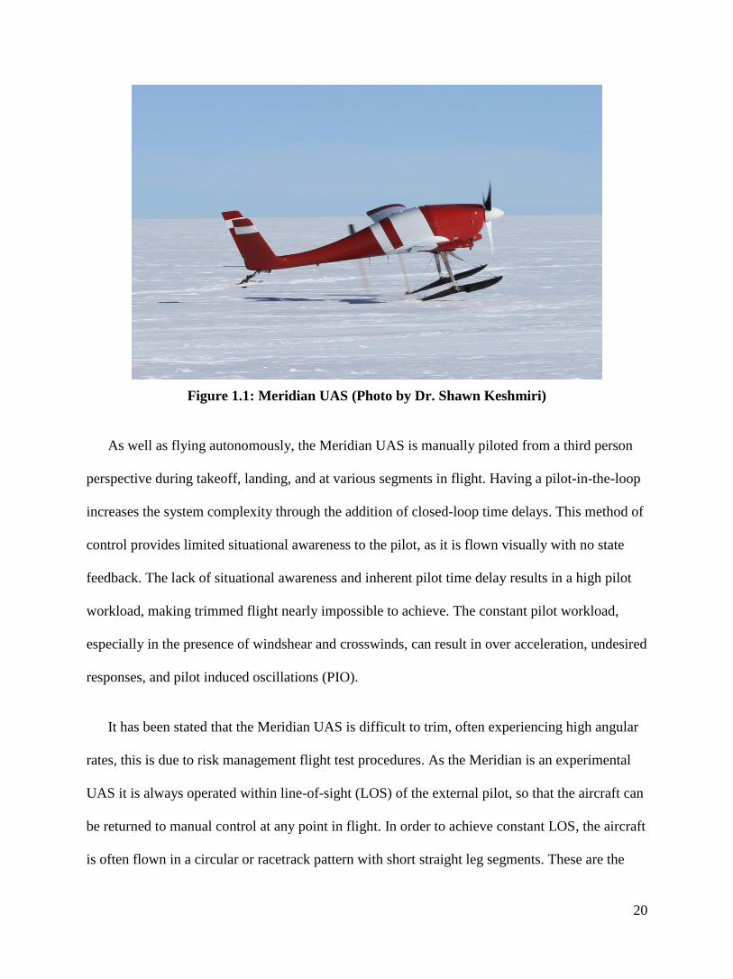
20
Figure 1.1: Meridian UAS (Photo by Dr. Shawn Keshmiri)
As well as flying autonomously, the Meridian UAS is manually piloted from a third person
perspective during takeoff, landing, and at various segments in flight. Having a pilot-in-the-loop
increases the system complexity through the addition of closed-loop time delays. This method of
control provides limited situational awareness to the pilot, as it is flown visually with no state
feedback. The lack of situational awareness and inherent pilot time delay results in a high pilot
workload, making trimmed flight nearly impossible to achieve. The constant pilot workload,
especially in the presence of windshear and crosswinds, can result in over acceleration, undesired
responses, and pilot induced oscillations (PIO).
It has been stated that the Meridian UAS is difficult to trim, often experiencing high angular
rates, this is due to risk management flight test procedures. As the Meridian is an experimental
UAS it is always operated within line-of-sight (LOS) of the external pilot, so that the aircraft can
be returned to manual control at any point in flight. In order to achieve constant LOS, the aircraft
is often flown in a circular or racetrack pattern with short straight leg segments. These are the
21
most demanding maneuvers to be commanded, as the aircraft in constant acceleration while
rolling and yawing, often at high bank and pitch angles, into and out of the wind. With the wind
direction constantly changing, due to aircraft orientation and windshear, the aerodynamics can
become unsteady and nonlinear [10].
The Meridian performed nine LOS flights between 2009 and 2011, both manually and
autonomously controlled, using the same autopilot for multiple configurations. The maiden
flight of the Meridian occurred on August 28, 2009 under manual control off of the Ft. Riley, KS
grass airfield, with no fairings and an unpainted airframe. This initial flight indicated that the
aircraft could fly in the draggiest configuration possible, serving as a proof of concept for the
experimental system. In September 2009 the Meridian performed three flights off of a paved
runway at Dugway Proving Grounds (DPG) without fairings, but with a partially painted
airframe. During these flight trials the aircraft performed brief autonomous flight segments for
the first time, revealing the low performance in maintaining the commanded altitude.
Following the DPG campaign the Meridian UAS traveled to Antarctica for its first polar
mission in December 2009, with a fully faired and painted airframe. The only Antarctic flight of
the season began with the external pilot performing a +5g pull-up while attempting to trim the
aircraft, resulting in a crack along the wing spar. The structural failure was not immediately
known though, and the flight continued with the aircraft flying autonomously for 10 minutes.
During the Antarctic flight it was further verified that the autopilot could not maintain altitude,
having a variation of ±40m.
In preparation for the summer 2011 Meridian deployment to NEEM camp in Greenland the
aircraft was equipped with ski gear, as to operate off of the snow runway. As a note, prior to
deployment the skis were trimmed while the aircraft was loaded; resulting in a ski pitch angle
22
above once the gear became unloaded. These flight tests served as a milestone, as this was
the first time that a working radar system had been flown onboard the Meridian. The radar
antennas were flat plate Vivaldi antennas that were incrementally attached spanwise along the
wing, inboard to outboard; with two antennas used for the second flight and four antennas
installed for the third flight. During the Greenland field campaign the Meridian performed three
flights, all of which experienced undamped oscillations during autonomous control. The third
flight performed the longest autonomous flight; however, the first two flights at NEEM are the
topic of discussion in this research, with the first flight including system identification
maneuvers to excite the Dutch Roll and short period modes. The second flight is the most
interesting of the three, as it included many commanded and uncommanded flight mode
transitions (i.e. RC, Manual, Home), and the aircraft experienced a loss of engine power shortly
during the last uncommanded transition. The final flight of the Meridian took place out of
Pegasus Airfield, Antarctica in December 2011, after performing its longest autonomous flight.
The flight tests of the Meridian have demonstrated that the aircraft was highly versatile and
resilient, having flown off of grass, paved, ice, and snow runways, experiencing high loading
maneuvers and landings, and performing an unpowered landing. However, the performance of
the closed-loop-system, both manually and autonomously controlled, indicated deficiencies
which require improvement in order to increase system reliability and performance to better
perform science missions.
The research presented in the forthcoming chapters presents dynamic analyses of the
Meridian UAS from flight test data. Model identification has been performed, from flight test
data, using Fuzzy Logic Modeling (FLM), which takes into account unsteady aerodynamics,
captures nonlinearity, and does not rely on predetermined functional relationships to generate
23
models. Chapter 2 presents an overview of the theoretical development used in this research,
serving as a literature review, which includes fundamental theories, data processing and analysis
techniques, and modeling methodologies. Chapter 3 presents discussion regarding a rudder
doublet performed in flight to assess directional stability and damping. Similarly Chapter 4
presents the effects of an elevator doublet performed in flight for longitudinal stability and
damping assessment. Chapter 5 addresses effects between manual flight and autonomous flight
transitions, as well as an investigation into unpowered flight performance. Chapter 6 summarizes
conclusions from the dynamic analyses and provides recommendations for future research.
24
2 Theoretical Development
The following sections serve as a literature review, presenting most equations,
derivations, and theories which were used during this research. The theoretical topics and
applications for all subsections are outlined as follows:
Section 2.1 Rigid Body Equations of Motion: The fundamentals of flight dynamics and
basis for generating physics based aircraft models and predicting dynamic response.
Section 2.2 Compatibility Analysis: Technique using kinematic relationships to remove
biases in flight test data prior to analysis.
Section 2.3 Equivalent Reduced Frequency: Application of Theodorsen’s theorem to
determine aerodynamic unsteadiness.
Section 2.4 Fuzzy Logic Modeling: Model identification technique for generating
nonlinear aircraft parameters as a function of the reduced frequency.
Section 2.5 Advanced Aircraft Analysis: Overview of the software’s linearized dynamic
modeling methodology and potential sources of error.
Section 2.6 Unsteady Aerodynamic and Vortex Theory: Fundamental theory
development and discussion of current unsteady aerodynamic and vortex research.
Section 2.7 Phase Angle Determination: Technique used to determine presence of PIO by
using Fourier integrals to determine if the aircraft motion is out of phase with control
inputs.
Section 2.8 Ruddervator Airflow Angles: Presentation of Current V-tail research and a
derivation which expands on the dihedral effect, without the assumption of small airflow
angles and accounts for the change in geometric angle of attack due to ruddervator
deflection.
25
2.1 Rigid Body Equations of Motion
Equations of motion for a rigid body aircraft are derived from Newton’s second law for
translational motion and Euler’s equation for rotational motion. The equations for Newton’s
second law and Euler’s equation, in the inertial frame, can be seen in equations 2.1 and 2.2
respectively.
( )
∑ 2.1
( )
∑ 2.2
The forces and moments due to aerodynamics, propulsion, and gravity act through the
aircraft center of gravity in the body centered coordinate system. Transforming the translational
and rotational equations of motion from the inertial frame to the body centered coordinate system
is performed through orthonormal transformation, using a cross-product-equivalent for angular
rotation. This transformation results in equations 2.3 and 2.4 respectively [17].
( )
∑ 2.3
( )
∑ 2.4
Since the flight time of the Meridian UAS is typically less than an hour, with a low
specific fuel consumption, it can be assumed that the change in mass and mass distribution is
“sufficiently small”, defined as a change of less than 5% during a 60 second period, resulting in
and
. Also it is assumed that the moment of inertia terms and will be
negligible, due to aircraft symmetry about the x-z plane [18]. With these assumptions applied,
26
the equations of motion can be expanded to six differential equations, one for each degree of
freedom, which can be seen in equations 2.5 and 2.6.
[
]
[ ( )
( )
( )
]
[
] [
]
[
]
2.5
[
] [
]
[[
] [
] [
] [ ]]
[ ( ) ( ) (
)
( ) ( )
(
) ( ) ( )
]
2.6
In the six degree of freedom (6DoF) equations of motion the unknowns are the
translational and rotational velocities which are solved through integrating the equations of
motion as a series of differential equations, due to cross-axis coupling, at each time step [17].
The body forces and moments are the forcing functions in the 6DoF equations of motion;
however, the body forces are resultants of lift and drag and must be modeled in the stability axis.
Linearized force and moment models are formulated as non-dimensional coefficients about a
steady state condition, which are expanded as first order Taylor series. The linearized models
assume a functional relationship of dominant states for the respective motion, as decoupled

27
motion is often assumed for linearization. The general equations for estimating aerodynamic
forces and moments for a V-tail configuration, equations 2.7 to 2.12, where the perturbed
airspeed coefficients are nondimensionalized by the steady state airspeed, , the longitudinal
rates are nondimensionalized by
, and the lateral-directional rates are nondimensionalized by
[18].
2.7
2.8
2.9
2.10
2.11
2.12
Furthermore, since classical modeling techniques assume the aircraft to be in steady state
flight with only small perturbations about the trim condition, model linearization will fail in
unsteady flight due to nonlinearity in the aerodynamic coefficients which cannot be modeled for
the steady state case. For marginally trimmed UAS flying in wind shear, high perturbations are
often encountered, resulting in model inaccuracies. These factors necessitate the use of nonlinear
force and moment models for UAS application [10].
As a final discussion regarding the equations of motion, the kinematic equations of
motion for both translational and rotational motion should be mentioned, where the translational
kinematic equations represent local position and the rotational kinematic equations represent
28
inertial attitude. The transformation matrix to transform from angular body rates to Euler angle
rates is composed of three orthonormal matrices; however, the complete transformation is not
orthonormal and has singularities at [17]. The rotational kinematic equations of
motion can be seen in equations 2.13 to 2.15.
2.13
2.14
( ) 2.15
2.2 Compatibility Analysis
Prior to performing fuzzy logic modeling a compatibility analysis must be performed, as the
estimated and measured states in flight (i.e. angular rates, accelerations, airflow angles, airspeed,
and attitude angles) generally have bias in their values due to both systematic errors and random
noise. Systematic error may be due to sensors being offset from the aircraft center of gravity,
sensor degradation over time, or poor calibration. In the case of Euler angle estimates, error may
also be due to inadequate covariance matrices within the Kalman filter. In order to properly
model aircraft dynamics, bias due to systematic error must be removed so that the error is not
propagated throughout the model; this is known as compatibility analysis [10] [19] [20].
Compatibility analysis determines the bias in measured data through the use of kinematic
relationships. Since the airflow angles are not measured in flight, they can be estimated during
compatibility analysis through the transformation of the translational body velocity to the
stability axis. The time derivatives of the airspeed, angle of attack, and sideslip angle must be
taken, as the analysis compares the rates of the kinematic relationships. The equations for the
translational velocities are shown in equation 2.16, while the equations for the total airspeed,
29
angle of attack, and sideslip angle, along with their respective time derivatives, can be seen
respectively in equations 2.17 to 2.19.
2.16
√ , 2.17
2.18
2.19
The translational stability axis kinematic equations are reformulated to have all force
terms replaced by accelerometer measurements. With the forces removed, all terms in equations
2.20 to 2.25 originate from measurements or estimations, which allows for systematic
uncertainty to be removed.
( ) ( )
( ) 2.20
( ) ( )
( ) 2.21
( ) ( )
( )
2.22
( ) 2.23

30
2.24
( ) 2.25
Biases are estimated for the twelve states in the sense of least squares through the
minimization of the square sum of the differences between the two sides of the six kinematic
equations. The six equations can be represented in vector form as shown in equation 2.26:
( ) ( ) 2.26
Where,
[ ] 2.27
[ ]
2.28
[
]
2.29
The cost function used to minimize the square sums is as shown in equation 2.30.
( ) ( ) 2.30
In the cost function the weighting matrix, Q, is a diagonal matrix with all weights set to
1.0, except for the airspeed weight which is set to 10.0 as it is a slow changing state [10]. Using
the measured data is estimated using a central difference scheme. The minimization of the cost
function must use the method of differential corrections due to the nonlinearity of the kinematic
functions, resulting in the iterative cost function shown in equation 2.31.
( )
( )
2.31
31
For each time instant the steps are repeated, up to 1000 times, until is determined and
then subtracted from the respective state at the given time [10] [19] [20]. This method allows for
the prediction of aircraft states which are not measured in flight, such as the angle of attack and
sideslip angle. With the biases removed from the data and unmeasured states predicted, the time
history for the total force and moment coefficient can be modeled, this research used previously
developed and proven code [21]. The force and moment coefficients are calculated using
equations 2.32 to 2.37, where the axial and pitching moment thrust contributions, and ,
are previously determined based on the altitude, airspeed, weight, and throttle position.
2.32
2.33
2.34
( ) ( )
2.35
( ) ( )
2.36
( ) ( )
2.37
2.3 Equivalent Reduced Frequency
The reduced frequency is of significance as it indicates the unsteadiness of the flow field
according to Theodorsen’s theory. Theodorsen’s theory derives the lift and pitching moment of
thin airfoils in unsteady incompressible flow experiencing small harmonic oscillations, where the
lift derivation is a function of both circulatory and noncirculatory terms. The Theodorsen
function used in these derivations is a complex function which uses Hankel functions of the
second kind and Bessel functions of the first and second kind, and is solely a function of the
32
reduced frequency. As the reduced frequency increases, the imaginary term in the Theodorsen
function increases and the real term decreases which leads to unsteady flow, reducing the
magnitude of the motion and inducing phase lag [22].
Since the motion is assumed to be harmonic, coupled equations are constructed to calculate
the reduced frequency in both the longitudinal and lateral-directional axes, where the angle of
attack and roll angle are the motions of interest for their respective axes. The coupled equations
are composed of the previously mentioned angles and their respective angular rates, both of
which are known values. The angle of attack and roll angle are assumed to oscillate about a mean
angle, represented by and respectively, at an angular frequency, , and phase angle, , with
a local amplitude, represented by and ; all of which are unknown values. The harmonic
equations are presented in equations 2.38 and 2.39 [10] [20] [23] [24].
[ ] [ ] 2.38
[ ] [ ] 2.39
Using the least squares optimization method, the cost function shown in equation 2.40 is
minimized and the unknowns in the previous equations can be calculated. In the cost function
can be replaced with to calculate the angular frequency of the rolling motion. Previously
developed and proven code was used to perform this [25].
∑ [ ( ( ))] ∑ [
( ( ))] 2.40
The angular frequencies calculated during the optimization process are directly related to
the reduced frequencies, where represents the reduced frequency of the pitching motion and
represents the reduced frequency of the rolling motion. A reduced frequency of 0 represents
steady aerodynamics, between 0 and 0.05 represents quasi-steady aerodynamics, and any value

33
beyond 0.05 is classified as unsteady [26]. The equations for the reduced frequencies can be seen
in equations 2.41 and 2.42; where due to the small chord length of the Meridian, is not
divided by 2, to keep the value from becoming too small.
2.41
2.42
2.4 Fuzzy Logic Modeling
Accurate dynamic aircraft models are essential to performing stability analysis, flight
controller development, and state estimation. However, model accuracy is limited by the
estimation techniques, as the assumptions made in these techniques do not hold true for the
Meridian UAS. Some of the common modeling techniques used for aircraft identification are
Least Squares (LS) Regression, Maximum Likelihood Estimation (MLE), and Stochastic
Modeling. LS regression is one of the most common techniques, often being linear, and
assuming that all unknown parameters are constant coefficients with random measurement noise.
LS regression is performed by relating a dependent variable to the sum of the regressors
multiplied by the modeled unknown constant coefficients. Although the implementation of this
method is fairly simple it requires a predetermined model structure, which may not be known
due to cross-coupling and disturbances. Also LS models are easily corrupted by measurement
noise, allowing for unknown disturbances and unsteady effects being propagated to the aircraft
model [27] [28].
MLE performs model optimization to determine the unknown parameters so that the
estimated values are “most likely” to occur based on the measured values. Often MLE uses
Extended Kalman Filters (EKF) to perform model estimation, as it is nonlinear and accounts for
34
Gaussian, white, and zero-mean noise. Although this method is nonlinear, it cannot accurately
model unsteady behavior with nonzero-mean oscillations. Finally stochastic models assume that
the unknown parameters are random variables which are estimated using Bayes’ rule. This
method is not widely used though as it requires predetermined functional relationships and a
priori probability density functions for the parameters [27] [28].
Flight test maneuvers and data collection occur in the time domain, and the previously
mentioned methods are often performed in the time domain, but identification can occur in the
frequency domain. Comprehensive Identification from Frequency Responses (CIFER),
developed by Dr. Mark Tischler, is an industry accepted application used in the development of
high fidelity models within the frequency domain. CIFER is able to determine the correlation of
the motion variables to other motion variables and control inputs, eliminating the need for
predetermined functional relationships. The data collection process for CIFER requires long
duration frequency sweeps of each control surface, with the aircraft starting and finishing in a
trim state [29]. This makes the data collection process difficult for Meridian analysis, as the pilot
rarely obtains trim and does not have enough time to command wide frequency spectrum
sweeps.
Due to the nonlinear and unsteady aerodynamic forces and moments acting on the aircraft,
conventional parameter identification methods are insufficient, as they produce time-invariant
steady models. It is difficult to determine the functional relationship between the measured states
and the estimated aerodynamic coefficients due to the previously mentioned time-dependent
nonlinear effects. Model identification, without the assumption of any functional relationships, is
possible through fuzzy logic modeling, developed by Dr. C.E. Lan [23] [24] [10] [20] [30]. FLM
is used to identify models, from flight test data, and appropriately weight each state with respect
35
to the aerodynamic coefficients, which leads to the calculation of stability and control derivatives
from the appropriately identified models.
The process of fuzzy logic modeling normalizes all input variables between 0 and 1 and each
motion variable is divided into multiple ranges, where each range represents a membership
function. These membership functions act as weights, also ranging from 0 to 1, for multiple
internal functions, where the internal functions are linear functions of input parameters. A weight
of 0 implies that there is no effect from the internal function, where as a weight of 1 implies that
there is a full effect. A fuzzy cell is defined as a membership function from each motion variable,
and each fuzzy cell contributes to the prediction of the internal function along with an associated
weight. The fuzzy rule states that if is ( ), and if is
( ), and … ,and is ( ),
then the cell output formulates the internal function shown in equation 2.43, where ( ) is the
membership function for the motion variable .
( )
2.43
In the equation 2.43, represents the aerodynamic force or moment coefficient being
modeled, and represents the motion variables for which the coefficient is functionalized, such
as angle of attack or reduced frequency. The coefficients of the internal functions are represented
by , where , and k is the number of input variables. The internal function
coefficients are iteratively determined through the minimization of the sum of squared errors
(SSE) between the model estimate and the actual data point, using the Newton gradient-descent
method shown in equations 2.44.
∑ ( )
2.44
36
The use of multiple internal functions is the source of the “fuzziness”, and the assembly
of these functions represents the model, capturing the nonlinear characteristics. The output of the
fuzzy logic model is the weighted average of the fuzzy cell outputs and is mathematically
represented by equation 2.45, with the index of cells being , where n is the total
number of cells, and the index of the data sets is , where m is the number of data
sets.
∑ [
( )
( ) ( )]
∑ [ ( )
( ) ( )]
2.45
As previously stated the minimization of the SSE is an iterative process which can be
performed using equation 2.46, where is a convergence factor.
( )
( )
∑ ( )
(
)
2.46
Equation 2.46 requires matrix iteration. In practice, this is often reduced to “point”
iteration for fast convergence [10]. The determining factor in the accuracy of the model
predictions is given by the multiple correlation coefficient, , shown in equation 2.47. In the
equation for , is the model prediction, is the measured data point, and is the mean of
the sample data.
∑ ( )
∑ ( )
2.47
2.5 Advanced Aircraft Analysis
It was previously mentioned that aircraft dynamic models are essential in performing
stability analysis, flight controller development, and state estimation. As such, formulation of
37
initial dynamic models must be performed prior to the collection of flight test data to ensure
aircraft stability. Preliminary models can be generated experimentally, theoretically, and
statistically, with all techniques having advantages and drawbacks. Experimental models are
generated through wind tunnel testing, which can measure both static and unsteady aerodynamic
forces and moments, with the latter using forced oscillation testing [31]. Wind tunnel testing is
often expensive though, due to the costs of scaled model acquisition and wind tunnel operation.
Theoretical models are generated using various computational fluid dynamic (CFD)
methods and software packages which can model pressure distribution, boundary layer thickness,
airflow velocity, and airflow angles through a control volume. Advanced CFD programs, such as
Fluent, uses the Navier-Stokes equations, shown in equations 2.50 to 2.52 in section 2.6, to
calculate the three-dimensional flow properties at various flight conditions. These nonlinear CFD
models are heavily dependent on proper surface grid meshing, with computation time dependent
on computer processing capabilities, often requiring parallel processing for complex models
[32]. In addition, predictive accuracy of stability derivatives by high-order CFD methods, in
particular all damping derivatives, has not been clearly demonstrated.
Low-fidelity CFD methods, such as the vortex lattice method, modify Prandtl’s lifting
line theory and model the flow interaction of all lifting surfaces as potential flow, using sheets of
horseshoe vortices. Vortex lattice methods assume that the lifting surfaces are thin, the airflow
angles are small, and the flow is incompressible, inviscid, and irrotational [33]. Dr. Mark Drela,
Terry J. Kohler Professor of Fluid Dynamics at MIT, has created and openly distributes the
vortex lattice software Athena Vortex Lattice (AVL) which allows users to rapidly generate
aircraft models based on geometry and flight conditions, neglecting fuselage interaction [34].
38
The statistical modeling method used in this research was performed through the software
Advanced Aircraft Analysis (AAA), which is industry accepted preliminary design software,
developed by DARCorporation. The theoretical foundation for this code is based on the theory
presented in Dr. Jan Roskam’s aircraft design, flight dynamics and controls, and performance
textbooks, the last of which is coauthored with Dr. C. E. Lan. AAA is capable of generating
linearized dynamic models of aircraft based entirely on specified aircraft flight condition,
geometry, and airfoil characteristics. Using statistical databases, most notably the digital
DATCOM, AAA interpolates amongst aerodynamic data for aircraft of different size with
similar configuration to generate fast, low-fidelity, preliminary dynamic models [35] [36].
With AVL and AAA being the tools of choice for rapidly generating preliminary models,
there are notable differences between the two, with varying performance levels. One such
difference is that AVL does not account for powered effects and assumes that all lifting surfaces
are thin, neglecting the fuselage interaction for non-slender bodies. Where AVL neglects non-
lifting surface items, AAA does not directly account for vortex interactions, using statistical
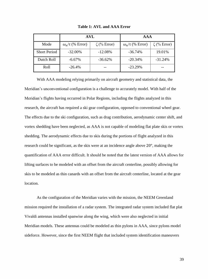
downwash and upwash angles to model vortex interaction. When compared against flight test
data for a small UAS, AVL and AAA predict the following maximum error bounds for the
natural frequency and damping ratio of the short period and Dutch roll modes and the time
constant of the roll mode, tabulated in Table 1[37]. Due to the large fuselage, power plant, and
unconventional configuration of the Meridian, AAA has been used as the primary preliminary
modeling software, which will further be discussed in this section.
39
Table 1: AVL and AAA Error
AVL AAA
Mode /τ (% Error) ζ (% Error) /τ (% Error) ζ (% Error)
Short Period -32.00% -12.08% -36.74% 19.01%
Dutch Roll -6.67% -36.62% -20.34% -31.24%
Roll -26.4% -- -23.29% --
With AAA modeling relying primarily on aircraft geometry and statistical data, the
Meridian’s unconventional configuration is a challenge to accurately model. With half of the
Meridian’s flights having occurred in Polar Regions, including the flights analyzed in this
research, the aircraft has required a ski gear configuration, opposed to conventional wheel gear.
The effects due to the ski configuration, such as drag contribution, aerodynamic center shift, and
vortex shedding have been neglected, as AAA is not capable of modeling flat plate skis or vortex
shedding. The aerodynamic effects due to skis during the portions of flight analyzed in this
research could be significant, as the skis were at an incidence angle above , making the
quantification of AAA error difficult. It should be noted that the latest version of AAA allows for
lifting surfaces to be modeled with an offset from the aircraft centerline, possibly allowing for
skis to be modeled as thin canards with an offset from the aircraft centerline, located at the gear
location.
As the configuration of the Meridian varies with the mission, the NEEM Greenland
mission required the installation of a radar system. The integrated radar system included flat plat
Vivaldi antennas installed spanwise along the wing, which were also neglected in initial
Meridian models. These antennas could be modeled as thin pylons in AAA, since pylons model
sideforce. However, since the first NEEM flight that included system identification maneuvers
40
had no installed antennas, no comparison has been made to AAA which requires antenna
modeling.
Before discussing sources of potential error in AAA modeling for the Meridian, two
shortcomings which affect model accuracy of small UAS will be addressed. The first of these
issues is that the database used for interpolation only extends to a Reynold’s number of ,
implying that for aircraft with small chord length and/or cruise speeds, the aerodynamic data is
extrapolated from the databases rather than interpolated. The second issue is that the zero lift
drag coefficient, , is often overestimated for aircraft with small wetted areas, as the
logarithmic relationship between parasite area and wetted area do not extend to low values and,
therefore, the effective parasite area is estimated to be larger than it is in actuality. However,
these modeling deficiencies should not affect modeling of the Meridian, as it is a large UAS near
the Reynold’s number boundary, with satisfied at airspeeds above 130 kts at
altitudes between 8000’ and 9000’ above mean sea level (AMSL).
The major contributor to error in the AAA Meridian model is that models are linearized
about a trim condition with no angular rates, which is a flight condition rarely attained in
Meridian flight. As previously discussed, the Meridian is an experimental aircraft requiring LOS
flight, so that the external ground pilot may regain command at any point in flight, to satisfy risk
management protocol. Due to the size and airspeed of the Meridian, LOS is achieved through
circular patterns which require constant pilot workload and often large control deflections,
resulting in constant, and often high, angular rates. As small motion perturbation is assumed in
AAA models, the portions of flight with high angular rates are not accurately modeled. However,
AAA does generate acceptable models for benign flight conditions near a trim condition, which
will be shown in following chapters.
41
2.6 Unsteady Aerodynamic and Vortex Theory
Aerodynamic theory is the basis for predicting forces and moments acting on an aircraft due
to airflow as well as the characteristics of the airflow. The purpose of this section is to
demonstrate the nonlinearities found in the governing equations for incompressible
aerodynamics through two- and three-dimensional aerodynamic and vortex theory, followed by a
discussion of unsteady aerodynamics. The governing equations of incompressible flow are
derived from two fundamental physical principles which must be satisfied: the continuity
equation and the momentum equation. The continuity equation states that mass can neither be
created nor destroyed, indicating that the mass flow rate into a control volume is equivalent to
the mass flow rate out of the control volume, as seen in equation 2.48 [38].
∰
∯
( ) 2.48
The momentum equation, Newton’s second law of motion, states that force is equivalent
to the time rate of change of momentum applied to a fluid. The unsteady, viscous flow,
momentum equation is represented in integral form by equation 2.49, and as three directional
component partial differential equations by equations 2.50 to 2.52, known as the Navier-Stokes
equations. The viscous forces are of interest as they include skin friction and pressure forces due
to unsteady effects such as boundary layer separation [38].
∰
∯ ( )
∯
∰
2.49
( )
( )
2.50
( )
( )
2.51
( )
( )
2.52
42
The aerodynamic definition of unsteadiness is described as differing pathlines of fluid
elements passing through the same point at different times, characterized by time varying airflow
properties. When the flow is steady all fluid elements have pathlines which are tangential to the
direction of the airflow, indicating a streamline invariant with time. Along the pathlines the
airflow velocity is free to rotate, generating vorticity; indicated by a nonzero value for the curl of
the velocity vector, as shown in equation 2.53.
2.53
Another rotational airflow characteristic is circulation, which is essential for lift
generation. Circulation is defined as the negative line integral of the air flow velocity around a
body, and subsequently is equivalent to the integral of the vorticity over an open surface bound
by the body for which circulation is occurring about. This is represented by equation 2.54, which
states that the negative circulation per unit span is equivalent to the vorticity component normal
to the surface element of the body [38].
( )
2.54
The concepts of vorticity and circulation, when applied to thin airfoil theory, state that an
infinitesimally small velocity at a given point is induced by a vortex sheet over a small section. A
vortex sheet is modeled as a series of vortex filaments, along a surface, with each vortex filament
having a sheet strength per distance along an infinitesimally small distance. As such, the vortex
sheet strength is only a function of the vortex filament strength tangential to the sheet, implying
that the normal velocity through the sheet is preserved with differential tangential velocities. This
assumption simplifies to equation 2.55, which states that the local vortex sheet strength is
equivalent to the local tangential velocity difference between the upper and lower surfaces.
43
2.55
For an airfoil, the circulation is the sum of the strength of the vortex sheet elements
around the airfoil given by equation 2.56.
∫ 2.56
The circulation about an airfoil is the essential flow property necessary for generating lift
along the chord line, given by the Kutta-Joukowski theorem in equation 2.57. The strength of the
vortex sheet, however, directly indicates the pressure difference between the upper and lower
surfaces, shown in equation 2.58 [38].
2.57
2.58
The discussion thus far only applies to airfoils, or infinite span wings, in a two-
dimensional flow, but in reality lifting surfaces are finite span wings in three-dimensional flow.
The third flow component is a spanwise element caused by the pressure difference, generated by
the circulation about the wing, resulting in air “spillage” over the wing tips. This spillage is
caused by the high pressure air on the lower surface traveling outboard along the wingspan,
attempting to reach a low pressure region, and eventually spilling over the wing tip. In an
opposite manner, air flowing along the upper surface moves inboard towards the wing root as the
high pressure air reaches the upper surface. As the air curls over the wing tip, the flow
interaction generates circulation, eventually forming strong vortices at each wing tip that
continue downstream [38].

44
The wing tip vortices bound the wing’s trailing flow, forming a trailing wake. According
to the Biot-Savart Law, the trailing wake is imposed with a downward velocity due to the
vorticity of the wing tip vortices, known as downwash. The downwash velocity generates an
induced angle of attack, which reduces the effectiveness of the relative angle of attack at the tail
surface [38]. Aircraft vortex generation is not limited to lifting surfaces; vortices are also shed
from the propeller blade tips, following a unique helical path. As such, the propeller generates
high propwash within the helical pattern, known as the slipstream. As the slipstream travels
downstream it comes in contact with the lifting surfaces, generating sidewash on the vertical tail
[39]. However, in the case of the Meridian, with the V-tail in the slipstream, it may better
describe the relative airflow as sidewash accompanied by upwash on the left surface and
downwash on the right surface.
The theory of vortex generation and downwash presented up to this point has only
examined the trailing wing wake and propeller slipstream, assuming that the aircraft is flying
into a constant wind field, in steady motion. These are essential theories for preliminary design,
determining steady trim values, and in performing static stability analysis; however, this does not
shed light on an aircraft’s dynamic response to vortex interaction. Dynamic motion can be
excited intentionally through control commands, or unintentionally through external
disturbances. As vortices are shed they travel downstream along the path of the relative wind, as
a result dynamic motion can occur due to windshear, crosswind, or flying into and out of the
wind [40].
An aircraft flying in a positive sideslip will have its tail located closer to the right wing
tip vortex, generating negative sidewash that produces an increases in the effective sideslip,
further stabilizing the motion [39]. In a similar fashion, aileron deflections change the pattern of
45
the vortices shed off the wing; specifically, the vortices shed from the up-deflected aileron
generate sidewash at the tail that creates a rolling moment which opposes the commanded
motion [39]. These examples of vortex interaction are defined for a conventional vertical tail; in
the case of a V-tail in a positive sideslip, the right surface will experience negative sidewash and
upwash that generates negative rolling, negative pitching, and positive yawing moments due to
cross-coupling and asymmetric loading across the V-tail.
The aircraft slipstream, while in a sideslip, can lead to dynamic stability degradation,
unlike the stabilizing wing tip vortices. This destabilizing effect begins to occur at a sideslip
angle that deflects the slipstream more over one half of a surface than the other half. As the
dynamic pressure of the slipstream is much larger than the free stream dynamic pressure, an
asymmetric pressure distribution occurs along the lifting surface, resulting in an uncommanded
rotation. For an aircraft in a positive sideslip, the increase in dynamic pressure along the left
wing surface results in a positive roll rate, with potential for the motion to be exacerbated if the
pilot improperly commands positive aileron [39]. Due to the adverse yaw effect a positive roll
rate would induce a negative yaw rate, which could result in further growth in the sideslip angle.
During this hypothetical roll and yaw motion, the left V-tail surface would experience greater
dynamic pressure than the right surface as well. The exact motion produced by the V-tail
pressure imbalance is difficult to determine; however, as the slipstream remains off-axis of the
aircraft centerline, motion about all three axes will occur, which could lead to oscillations.
Serious roll oscillation can result from windshear as the time variation in sideslip can contribute
to large unstable roll damping (i.e.
derivatives) and thus PIO.
Oscillatory motion serves as an indicator of nonlinear and unsteady aerodynamics,
developing due to both commanded and uncommanded flow asymmetries. Unsteady

46
aerodynamics often occur at high airflow angles or in the presence of atmospheric turbulence as
a result of time-dependent boundary layers and vortex wakes, dynamic stall, vortex bursting, and
vortex lag [23]. Unsteady aerodynamic motions can include oscillatory wing rock, asymmetric
loss of lift in wing drop, loss of stability or control reversal, and can even develop into loss of
control such as a spiral [17].
The constant maneuvering of the Meridian increases the risk for dynamic stall
development, due to the high angular rates creating large changes in the effective angle of attack.
Dynamic stall begins with a transient delay in separation followed by the formation of a dynamic
stall vortex, which may temporarily increase lift. As the dynamic stall vortex sheds and
propagates across the wing there is an abrupt and unsteady change in the generated forces and
moments [41]. The vortex structure generated during an unsteady roll can be thought of as a
plunging motion, as both motions are normal to the free stream. During a down stroke the
trailing wing tip vortex breakdowns into a double-helix with opposite rotation, while at the same
time a leading edge vortex is formed at the wing tip. As the motion continues, the transverse
velocity along the wing towards the centerline increases, with the leading edge vortex beginning
to detach from the wing surface, forming a semi-arc, that remains pinned at the leading edge. At
the end of the stroke the leading edge vortex completely separates and travels downstream with
an arc-like structure. The upstroke is very similar, however, the transverse velocity direction is
opposite and the leading edge vortex forms along the lower surface, due to the negative angle of
attack [42] [43].
Similar to the plunging motion, an unsteady pitch will form leading edge vortices (or
called shedding vortices) attached at the wing tips. The transverse velocity towards the centerline
begins to increase as the pitching motion continues, and the leading edge vortices will begin to

47
breakdown. The two leading edge vortices will eventually come together at the centerline,
forming an arc with a large-scale swirling pattern. As the angle of attack increases the arc vortex,
unlike during a plunging motion, remains attached to the surface, creating suction as break down
occurs [41] [44]. Furthermore, skin friction drag is independent of the motion frequency, making
it possible to generate thrust instead of drag at high enough frequencies and oscillation
magnitudes [45]. This is best illustrated by a swimmer moving though water entirely by the use
of oscillatory leg movements, without the use of their hands.
The aerodynamic theory presented in this section will be applied in the forthcoming
chapters to explain uncommanded motion and nonlinear effects. The subject of unsteady
aerodynamics has seen much research in recent years, through both forced oscillation wind
tunnel tests and CFD simulations. Since nonlinear and unsteady aerodynamics cannot be
generalized in application, the presented literature review focused on unsteady aerodynamic
motions of airfoils and low aspect ratio rectangular wings.
2.7 Phase Angle Determination for Control-Induced Oscillation
Control-induced oscillation, known as PIO, is defined by the Military Handbook 1797A as
being “sustained or uncontrollable oscillation resulting from the efforts of the pilot to control the
aircraft” [46]. The occurrence of PIO is often associated with aircraft deficiencies such as
sluggish, nonlinear, or coupled control responses and unstable or lightly damped dynamic modes
[47]. Between 1996 and 2004 sixteen documented PIO incidents have occurred in civil,
transport, and military aircraft; resulting in ten fatalities, millions of dollars spent on aircraft
repairs and court fees, and even the indictment of one pilot [48]. Although the frequency of PIO
related incidents is low in manned aircraft, UAS are more prone to experiencing PIO due to
communication system latency, actuator time delay, and unsteady aerodynamic lag [49]. As well
48
as system deficiencies, a 2004 report documented that military UAS accidents due to human
factors, including PIO, account for 20% to 67% of all incidents. Of these incidents due to human
factors, 67% to 78% occur during takeoff and landing, where PIO is most likely to occur [50].
The presence of PIO due to human factors can be attributed to the inherent time delay of the
pilot-in-the-loop, stemming from the pilot’s lack of total situational awareness and inability to
physically feel the force feedback on the control stick and aircraft response [51].
As PIO is a sustained and uncontrolled oscillation, the motion can be constant in amplitude,
convergent, or even divergent, with no requirement on the minimum number of cycle oscillations
[48]. This oscillatory motion is due to the pilot commanding control surface deflections at
frequencies that are out of phase with the frequency of the aircraft response. This leads to the
first criteria used for detecting PIO, which is that the aircraft motion and pilot control commands
will have a phase shift of for aircraft attitude angles and a phase shift of for the aircraft
angular rates [48].
The other two criteria used in identifying PIO state that the frequency of the oscillatory
motion must be at a reasonably high frequency and the amplitude of the motion must be
sufficiently large. The determination of thresholds which satisfy the frequency and amplitude
criteria have been generalized to expected ranges, however, these thresholds vary for different
aircraft. It is commonly accepted that the frequency of the PIO should fall within the range of the
pilot command frequency, often between
and
, with peak-to-peak control deflections
greater than 4° [47] [48]. The motion amplitude thresholds, however, are dependent on the
various oscillatory modes, known as roll ratchet/yaw chatter, pitch bobble, and high-frequency
pitch PIOs, as well as pitch, roll, and yaw PIOs; shown in
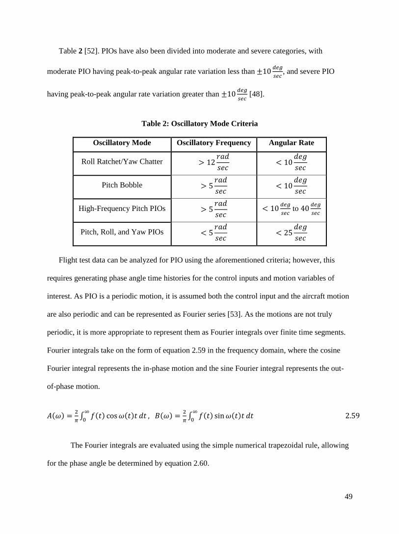
49
Table 2 [52]. PIOs have also been divided into moderate and severe categories, with
moderate PIO having peak-to-peak angular rate variation less than
, and severe PIO
having peak-to-peak angular rate variation greater than
[48].
Table 2: Oscillatory Mode Criteria
Oscillatory Mode Oscillatory Frequency Angular Rate
Roll Ratchet/Yaw Chatter
Pitch Bobble
High-Frequency Pitch PIOs
to
Pitch, Roll, and Yaw PIOs
Flight test data can be analyzed for PIO using the aforementioned criteria; however, this
requires generating phase angle time histories for the control inputs and motion variables of
interest. As PIO is a periodic motion, it is assumed both the control input and the aircraft motion
are also periodic and can be represented as Fourier series [53]. As the motions are not truly
periodic, it is more appropriate to represent them as Fourier integrals over finite time segments.
Fourier integrals take on the form of equation 2.59 in the frequency domain, where the cosine
Fourier integral represents the in-phase motion and the sine Fourier integral represents the out-
of-phase motion.
( )
∫ ( ) ( )
( )
∫ ( ) ( )
2.59
The Fourier integrals are evaluated using the simple numerical trapezoidal rule, allowing
for the phase angle be determined by equation 2.60.
50
( )
2.60
Using the generalized mathematical form, the Fourier integrals are determined using
equations 2.61 and 2.62, while the phase angle is determined using equation 2.63, for both the
roll angle and aileron input. The example equations given below apply to the roll angle and
aileron input, however, these equations are valid for all control inputs and respective dominate
states.
∫ ( ) ( )
∫ ( ) ( )
2.61
∫ ( ) ( )
∫ ( ) ( )
2.62
( )
( )
2.63
In the previous equations the angular frequency, ω, is determined from the lateral-
directional reduced frequency, . The phase shift used to identify PIOs is determined by the
difference between the roll angle phase and the aileron phase. For negative phase shifts 360° is
added so that all results are positive. These equations can be used to calculate the phase of
different control surfaces and motion variables, using to determine the angular frequency of
longitudinal motion.
2.8 Ruddervator Airflow Angles
The V-tail configuration, with full moving ruddervators, is a challenging control problem to
solve due to cross-coupling between longitudinal and lateral-directional motion. Historically the
V-tail configuration has not been widely used; the most notable implementation was on the
Beech Bonanza. Though the Beech Bonanza V-tail configuration was in production for many
years the production stopped in 1982, as there was a large history of fatal accidents due to both
the difficulty of managing the cross-coupling and mid-air breakups due to large stress on the
51
empennage. The V-tail has recently become popular in the UAS industry, with the advancement
of digital flight controllers, as it offers weight and drag reductions which can potentially increase
performance [39].
Due to the low popularity in the V-tail configuration, limited publications exist on
developing accurate aerodynamic models of the V-tail surfaces. Dr. Phillips, from Utah State
University, has formulated a V-tail model based on dihedral effect theory and has performed
simple aerodynamic analysis using Prandtl’s lifting-line theory [54]. The work performed by
Phillips has set a foundation for V-tail research; however, his research assumes a fixed incidence
angle for each V-tail surface, neglecting asymmetric surface deflections and flow interactions
between the surfaces. These simple aerodynamic models have been implemented in recent
versions of AAA; however, the geometric V-tail model used in AAA is inconsistent with the
geometric definition of Phillips’ formulation [35]. Phillips’ formulation models each surface
separately and combines the models to form a complete V-tail model, where AAA models the V-
tail as an entire lifting surface. Therefore, the difference between Phillips’ and AAA’s geometric
definitions is that AAA calculates the planform span and surface area as a horizontal projection
of the V-tail, where Phillips calculates the true span and surface area of each surface. The V-tail
analyses performed in this research expand on Phillips’ model, without assuming small angles,
through the inclusion of ruddervator deflection angles in determining the airflow angles at each
surface.
Inaccuracies in V-tail modeling are not limited to aerodynamic force and moment estimation,
but can be seen in control system design. The Meridian UAS control system assumes that there is
negligible control cross-coupling and decomposes the ruddervator commands into an elevator
and rudder command based on the horizontal and vertical projections of the V-tail. The control
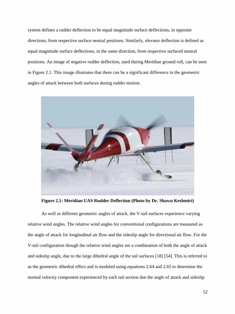
52
system defines a rudder deflection to be equal magnitude surface deflections, in opposite
directions, from respective surface neutral positions. Similarly, elevator deflection is defined as
equal magnitude surface deflections, in the same direction, from respective surfaced neutral
positions. An image of negative rudder deflection, used during Meridian ground roll, can be seen
in Figure 2.1. This image illustrates that there can be a significant difference in the geometric
angles of attack between both surfaces during rudder motion.
Figure 2.1: Meridian UAS Rudder Deflection (Photo by Dr. Shawn Keshmiri)
As well as different geometric angles of attack, the V-tail surfaces experience varying
relative wind angles. The relative wind angles for conventional configurations are measured as
the angle of attack for longitudinal air flow and the sideslip angle for directional air flow. For the
V-tail configuration though the relative wind angles are a combination of both the angle of attack
and sideslip angle, due to the large dihedral angle of the tail surfaces [18] [54]. This is referred to
as the geometric dihedral effect and is modeled using equations 2.64 and 2.65 to determine the
normal velocity component experienced by each tail section due the angle of attack and sideslip

53
angles. It should be noted that the airflow angles and velocity in the following equations are not
the free stream values, but rather what is coming into contact with the tail after downwash and
sidewash contributions.
2.64
2.65
Small angle assumptions are usually applied when modeling the dihedral effect, however,
at this time no assumptions will be used in the derivation as it is of interest to investigate effects
due to large airflow angles. Using the normal velocity components for each tail section the
relative airflow angle, represented by , can be calculated with respect to the x-body velocity,
, using equations 2.66 and 2.67. It is important to state that this is not the angle
of attack in a conventional sense; it is a combination of the incoming angle of attack and sideslip
angle, occurring in the plane defined by the x-body velocity and the velocity vector normal to the
surface.
(
) (
)
(
) 2.66
(
) (
)
(
) 2.67
The airflow angles are not simply a function of the relative airflow angle, but are also
affected by the V-tail incidence angle and the ruddervator deflections about the incidence angle.
With the inclusion of the geometric angles of attack, the angle of attack and sideslip angle of

54
each surface are calculated through a simple transformation about the dihedral angle. In
equations 2.68 to 2.71 positive ruddervator deflection and V-tail incidence are defined as leading
edge up, resulting in the transformation for and to occur about , to
occur about , and occurs about ( ).
( )( ) 2.68
( )( ) 2.69
( )( ) 2.70
( )( ) 2.71
Using these modified airflow angles the lift and sideforce coefficients are formulated for
both V-tail sections. The lift curve slope is assumed to be equivalent to the lift curve slope of a
horizontal projection of the planform with no dihedral. When estimating the lift curve slope of
the v-tail it is necessary to include effects due to the V-tail sweep angle. Since the Meridian’s V-
tail uses symmetric NACA 0012 airfoils the lift curve slope is the same for the calculation of lift
and sideforce. Equations 2.72 to 2.75 represent the lift and sideforce equations for each surface,
with respective coefficients:
⁄
2.72
⁄
2.73
⁄
2.74
⁄
2.75
These models aid in showing the trends of the lift and sideforce generated by the V-tail,
but in the scope of this research, they fail to accurately model these forces. The uncertainty in the

55
direction and velocity of the airflow interacting with the V-tail is large and time-dependent, due
to the downstream unsteady flow. The free stream flow is altered by the unsteady aerodynamic
effects of the propwash, trailing edge vortices, cross wind, and fuselage flow separation.
Additional error in the modeled aerodynamic forces can be attributed to the flow interaction
imposed on each V-Tail surface by the other surface, due to changing airflow direction and
surface deflections. Thorough research with regards to surface flow interactions has not been
performed and cannot be assumed negligible, as it is not considered negligible for a conventional
tail configuration.

56
3 Rudder Doublet Analysis
During the first NEEM flight a rudder doublet was performed to assess the directional
stability and damping of the aircraft. Subsequently this motion sheds light on some cross-coupled
motions due to the V-tail configuration. Preceding the rudder doublet, controlled maneuvers
were made in attempt to trim the aircraft, followed by the return of all control surfaces to neutral
positions so to reduce motion not induced by rudder deflections. The following subsections will
begin with addressing the pilot commanded maneuvers while trimming the aircraft, followed by
discussion of the dynamic effects induced by the rudder doublet, finishing with an evaluation of
the linearized models developed for a Dutch roll motion.
3.1 Aileron Commanded Trim Maneuver
Prior to the rudder doublet, the pilot began to input aileron commands so to level the
wings. Instead of holding a constant aileron command, the pilot performed three aileron cycles
between t = 0.3 seconds to t = 1.5 seconds with deflections ranging from to . During this
motion the roll damping stability term, ( ), varied between positive and negative, an
indicator that the aircraft is periodically gaining roll energy due to this oscillatory unsteady
motion, shown in Figure 3.1. The nonlinear oscillatory roll damping derivative, ( ), serves as
an indicator of an increase in energy per roll cycle when positive, as it is no longer working as an
effective damper, shown in equation 3.1 [10].
( )
3.1

57
Figure 3.1: Aileron Commanded Unsteady Rolling Motion
During this cyclical aileron input PIO occurred in the rolling motion over a short time
period of 1.6 seconds. The existence of this PIO is identified by an average phase shift of 179.7°
between the roll angle and the aileron input, shown in Figure 3.2; this is accompanied by a peak-
to-peak variation in the roll rate and aileron deflection of 15 deg/s and , respectively. The
nonlinear effect resulting from this PIO is seen in the form of roll rate reversal, as the pilot
commands positive roll rate throughout the maneuver. At t = 1 second the roll rate reverses from
positive to negative due to the unsteady motion, which is further illustrated by the increased roll
energy. Once the pilot ceases aileron input the roll damping derivative returns to a stable value
and the roll rate goes to zero. Though the duration of this PIO is short, it illustrates the nonlinear
and unsteady aerodynamic effects created through high frequency and large amplitude control
inputs, such as uncommanded motion, which could lead to aircraft instability.
0 0.2 0.4 0.6 0.8 1 1.2 1.4 1.6 1.8-10
0
10
Time (sec)p (
deg/s
)
0.2 0.4 0.6 0.8 1 1.2 1.4 1.6 1.8
-10123
Time (sec)
a (
deg)
0 0.2 0.4 0.6 0.8 1 1.2 1.4 1.6 1.8-10
-5
0
Time (sec)
(
deg)
0.2 0.4 0.6 0.8 1 1.2 1.4 1.6 1.8
-1
0
1
Time (sec)
Clp
(osc)
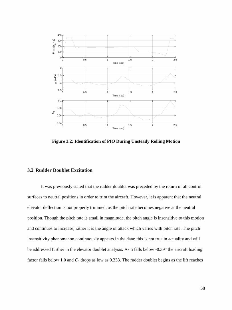
58
Figure 3.2: Identification of PIO During Unsteady Rolling Motion
3.2 Rudder Doublet Excitation
It was previously stated that the rudder doublet was preceded by the return of all control
surfaces to neutral positions in order to trim the aircraft. However, it is apparent that the neutral
elevator deflection is not properly trimmed, as the pitch rate becomes negative at the neutral
position. Though the pitch rate is small in magnitude, the pitch angle is insensitive to this motion
and continues to increase; rather it is the angle of attack which varies with pitch rate. The pitch
insensitivity phenomenon continuously appears in the data; this is not true in actuality and will
be addressed further in the elevator doublet analysis. As α falls below -0.39° the aircraft loading
factor falls below 1.0 and drops as low as 0.333. The rudder doublet begins as the lift reaches
0 0.5 1 1.5 2 2.50
100
200
300
400
Time (sec)
Phase(
a -
)
0 0.5 1 1.5 2 2.50.5
1
1.5
2
Time (sec)
(
rad/s
)
0 0.5 1 1.5 2 2.50.04
0.06
0.08
0.1
Time (sec)
K2

59
a minimum value and instantaneously increases to 0.388, though α continues to decrease, as
shown in Figure 3.3.
Figure 3.3: Pitch Insensitivity and Loss of Lift at Neutral Control Position
The rudder doublet began after t = 2.1 seconds and was returned to the neutral position at
t = 3.7 seconds, with maximum deflections of 5.85° and -7.65° during this cycle. As deflects
in the positive direction, the yaw rate is unchanged for the first 0.4 seconds, indicating a
significant aerodynamic lag that could result in directional PIO for an unaware pilot. When
compared against the rate of it shows that the yaw rate begins to react as the rate becomes
negative, shown in Figure 3.4.
0 0.5 1 1.5 2 2.5 3 3.5 4 4.5 5-20
0
20
Time (sec)
q (
deg/s
)
0 0.5 1 1.5 2 2.5 3 3.5 4 4.5 5-10
0
10
Time (sec)
(
deg)
0 0.5 1 1.5 2 2.5 3 3.5 4 4.5 5-10
-5
0
Time (sec)
(
deg)
0 0.5 1 1.5 2 2.5 3 3.5 4 4.5 50
0.5
1
Time (sec)
Cz
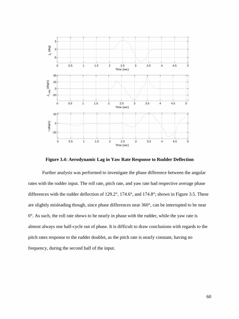
60
Figure 3.4: Aerodynamic Lag in Yaw Rate Response to Rudder Deflection
Further analysis was performed to investigate the phase difference between the angular
rates with the rudder input. The roll rate, pitch rate, and yaw rate had respective average phase
differences with the rudder deflection of 129.2°, 174.6°, and 174.8°; shown in Figure 3.5. These
are slightly misleading though, since phase differences near 360°, can be interrupted to be near
0°. As such, the roll rate shows to be nearly in phase with the rudder, while the yaw rate is
almost always one half-cycle out of phase. It is difficult to draw conclusions with regards to the
pitch rates response to the rudder doublet, as the pitch rate is nearly constant, having no
frequency, during the second half of the input.
0 0.5 1 1.5 2 2.5 3 3.5 4 4.5 5
-5
0
5
Time (sec)
r (
deg)
0 0.5 1 1.5 2 2.5 3 3.5 4 4.5 5
-20
0
20
40
Time (sec)
r-
dot (
deg/s
)
0 0.5 1 1.5 2 2.5 3 3.5 4 4.5 5
-20
0
20
Time (sec)
r (d
eg/s
)
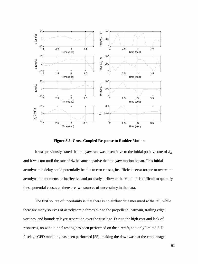
61
Figure 3.5: Cross Coupled Response to Rudder Motion
It was previously stated that the yaw rate was insensitive to the initial positive rate of
and it was not until the rate of became negative that the yaw motion began. This initial
aerodynamic delay could potentially be due to two causes, insufficient servo torque to overcome
aerodynamic moments or ineffective and unsteady airflow at the V-tail. It is difficult to quantify
these potential causes as there are two sources of uncertainty in the data.
The first source of uncertainty is that there is no airflow data measured at the tail, while
there are many sources of aerodynamic forces due to the propeller slipstream, trailing edge
vortices, and boundary layer separation over the fuselage. Due to the high cost and lack of
resources, no wind tunnel testing has been performed on the aircraft, and only limited 2-D
fuselage CFD modeling has been performed [55], making the downwash at the empennage
2 2.5 3 3.5-20
0
20
Time (sec)
p (
deg/s
)
2 2.5 3 3.50
200
400
Time (sec)
Phase(
r - p
)
2 2.5 3 3.5-10
0
10
Time (sec)
q (
deg/s
)
2 2.5 3 3.50
200
400
Time (sec)
Phase(
r - q
)2 2.5 3 3.5
-50
0
50
Time (sec)
r (d
eg/s
)
2 2.5 3 3.50
200
400
Time (sec)P
hase(
r - r
)
2 2.5 3 3.5-10
0
10
Time (sec)
r (
deg/s
)
2 2.5 3 3.50
0.05
0.1
Time (sec)
k2
62
difficult to estimate. The second source of uncertainty is that there is no state feedback on the
aircraft control deflections, and it is assumed that the deflection is equivalent to the commanded
value. If the moments generated by the rudder deflection command are not sufficient to
overcome the aerodynamic moments there would be no rudder deflection, resulting in no yaw
rate generation until the aerodynamic moments were overcome. The data, however, would
incorrectly show it to be the commanded value.
Although, due to limited recorded data, it is impossible to prove that the aerodynamic
moments acting on the tail exceed the servo limitations, it is worth introducing the idea for future
research. During Meridian ground testing it was observed that the right ruddervator could be
moved by hand when the servos were not powered. This is concerning because the servos are
screw driven and should lock in position; when loaded with aerodynamic forces, in particular the
oscillatory ones, the potential exists for the screw drives to slip, which could lead to deflections
different from the commanded value or flutter. The existence of insufficient servo torque to
perform rudder deflection is illustrated through a second order linearized moment balance model
at the rudder hinge-line. The linearized differential equation of the moment balance can be seen
in equation 3.2 as a function of the rudder deflection rate, rudder deflection angle, sideslip angle,
and their respective effective specific moments. The effective specific moments, represented
by , physically represent the moment per unit of moment of inertia, or rather the sensitivity of
the specific moment to the respective motion variable [17].
3.2
The linearized differential equation of rudder moment balance can be decomposed into
two first order differential equations shown in equation 3.3 to 3.5.

63
[
] [
] 3.3
3.4
3.5
Using the derived first order differential equations, the Coulomb friction function can be
implemented. The Coulomb friction function models a constant external hinge-moment,
represented by , that opposes the direction of rudder motion and counters the generated rudder
moments. The Coulomb friction function is described by equation 3.6.
| | 3.6
Substituting the Coulomb friction function into the equation for yields the inequality
shown in equation 3.7, since the hinge-moment generated by the rudder must overcome the
external moments.
| | 3.7
The implication of this inequality is that if the external moments acting on the rudder are
greater than the hinge-moment generated by the rudder, then the rudder is in a “dead zone” and
no effective moments are generated. Further hinge-moment analysis should be performed as
large aerodynamic moments could result in servo failure if continuous loading exceeds the
manufacturer’s operational range, however, at this time it is out of the scope of this research.
The cause for the yaw rate delay is most likely due to the large lateral-directional
unsteady flow generated during the maneuver to trim level the wings. The oscillatory yaw
damping, ( ), and sideforce damping, ( )
, terms should be opposite in sign, as the
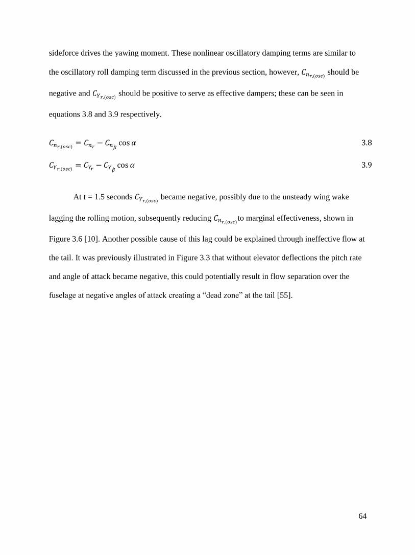
64
sideforce drives the yawing moment. These nonlinear oscillatory damping terms are similar to
the oscillatory roll damping term discussed in the previous section, however, ( ) should be
negative and ( ) should be positive to serve as effective dampers; these can be seen in
equations 3.8 and 3.9 respectively.
( )
3.8
( )
3.9
At t = 1.5 seconds ( ) became negative, possibly due to the unsteady wing wake
lagging the rolling motion, subsequently reducing ( )to marginal effectiveness, shown in
Figure 3.6 [10]. Another possible cause of this lag could be explained through ineffective flow at
the tail. It was previously illustrated in Figure 3.3 that without elevator deflections the pitch rate
and angle of attack became negative, this could potentially result in flow separation over the
fuselage at negative angles of attack creating a “dead zone” at the tail [55].
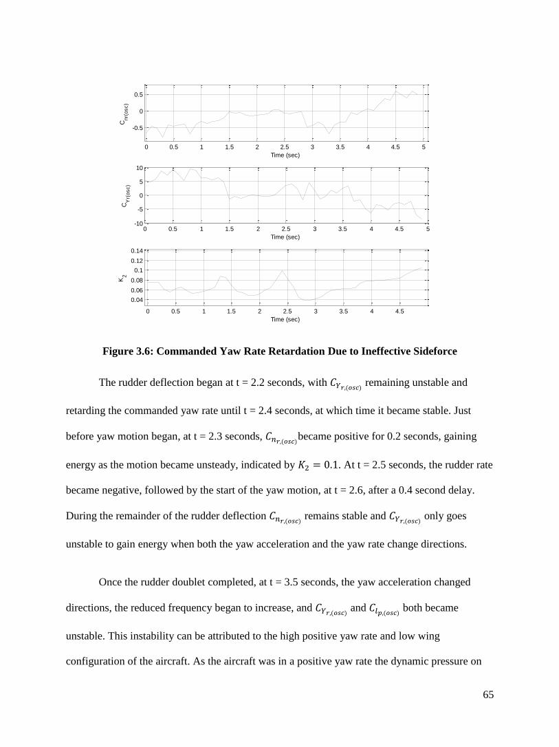
65
Figure 3.6: Commanded Yaw Rate Retardation Due to Ineffective Sideforce
The rudder deflection began at t = 2.2 seconds, with ( ) remaining unstable and
retarding the commanded yaw rate until t = 2.4 seconds, at which time it became stable. Just
before yaw motion began, at t = 2.3 seconds, ( )became positive for 0.2 seconds, gaining
energy as the motion became unsteady, indicated by . At t = 2.5 seconds, the rudder rate
became negative, followed by the start of the yaw motion, at t = 2.6, after a 0.4 second delay.
During the remainder of the rudder deflection ( ) remains stable and ( )
only goes
unstable to gain energy when both the yaw acceleration and the yaw rate change directions.
Once the rudder doublet completed, at t = 3.5 seconds, the yaw acceleration changed
directions, the reduced frequency began to increase, and ( ) and ( )
both became
unstable. This instability can be attributed to the high positive yaw rate and low wing
configuration of the aircraft. As the aircraft was in a positive yaw rate the dynamic pressure on
0 0.5 1 1.5 2 2.5 3 3.5 4 4.5 5
-0.5
0
0.5
Time (sec)
Cnr(
osc)
0 0.5 1 1.5 2 2.5 3 3.5 4 4.5 5-10
-5
0
5
10
Time (sec)
CY
r(osc)
0 0.5 1 1.5 2 2.5 3 3.5 4 4.5
0.04
0.06
0.08
0.1
0.12
0.14
Time (sec)
K2
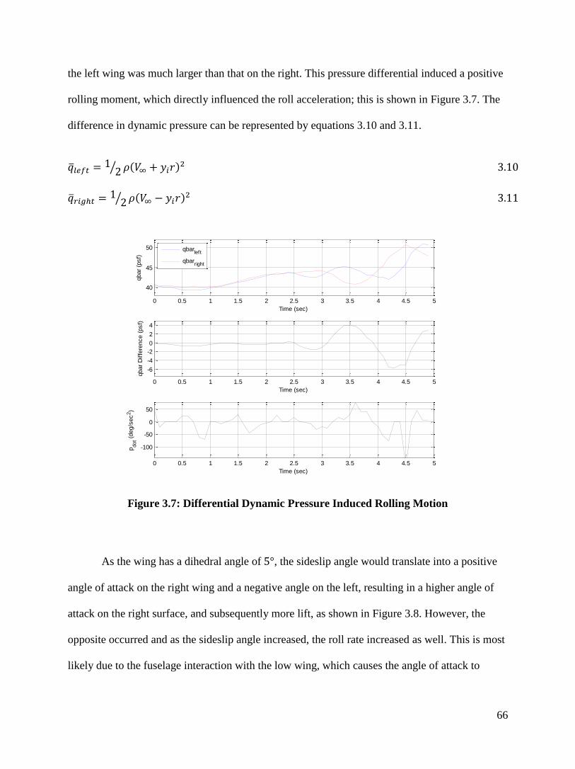
66
the left wing was much larger than that on the right. This pressure differential induced a positive
rolling moment, which directly influenced the roll acceleration; this is shown in Figure 3.7. The
difference in dynamic pressure can be represented by equations 3.10 and 3.11.
⁄ ( )
3.10
⁄ ( )
3.11
Figure 3.7: Differential Dynamic Pressure Induced Rolling Motion
As the wing has a dihedral angle of , the sideslip angle would translate into a positive
angle of attack on the right wing and a negative angle on the left, resulting in a higher angle of
attack on the right surface, and subsequently more lift, as shown in Figure 3.8. However, the
opposite occurred and as the sideslip angle increased, the roll rate increased as well. This is most
likely due to the fuselage interaction with the low wing, which causes the angle of attack to
0 0.5 1 1.5 2 2.5 3 3.5 4 4.5 5
40
45
50
Time (sec)
qbar
(psf)
qbarleft
qbarright
0 0.5 1 1.5 2 2.5 3 3.5 4 4.5 5
-6
-4
-2
0
2
4
Time (sec)
qbar
Diffe
rence (
psf)
0 0.5 1 1.5 2 2.5 3 3.5 4 4.5 5
-100
-50
0
50
Time (sec)
pdot (
deg/s
ec
2)

67
decrease on the right wing and increase on the left wing during positive sideslip, creating a
destabilizing effect instead of stabilizing.
Figure 3.8: Dihedral Effect Difference in Angle of Attack Ineffective Damping
As the yaw rate became increasingly negative the roll rate remained positive and the roll
angle began to grow. The difference in the left and right wing dynamic pressures slowed the roll
rate, though it remained positive, and the lift coefficient began to decrease as increased. As
the unsteady loss of lift continued, a rapid increase in roll angle and decrease in the angle of
attack occurred; shown in Figure 3.9. At this instant, ( ) became unstable as the yaw rate
increased from ⁄ to ⁄ during one cycle when damping should occur. As discussed in
Section 2.6, the sideslip angle, along with a large magnitude cross wind, displaced the slipstream
more over the left V-tail surface than the right. This resulted in the destabilizing effect of
generating a higher dynamic pressure on the left surface that created the negative yaw rate and
positive roll rate, illustrated in Figure 3.10.
0 0.5 1 1.5 2 2.5 3 3.5 4 4.5 5
-5
0
5
Time (sec)
(
deg)
left
right
0 0.5 1 1.5 2 2.5 3 3.5 4 4.5 5-0.5
0
0.5
1
1.5
Time (sec)
D
iffe
rence (
deg)
0 0.5 1 1.5 2 2.5 3 3.5 4 4.5 5-10
0
10
20
Time (sec)
p(d
eg/s
ec)
0 0.5 1 1.5 2 2.5 3 3.5 4 4.5 5-4-202468
Time (sec)
(
deg)
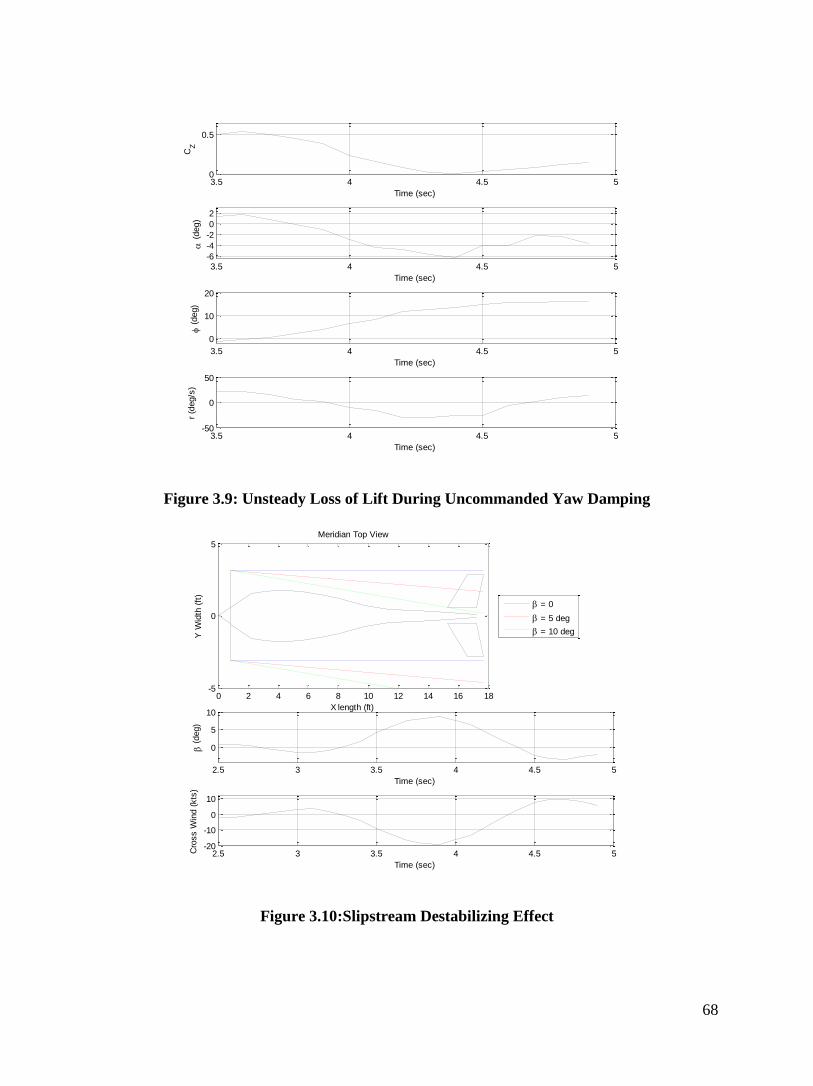
68
Figure 3.9: Unsteady Loss of Lift During Uncommanded Yaw Damping
Figure 3.10:Slipstream Destabilizing Effect
3.5 4 4.5 50
0.5
Time (sec)C
Z
3.5 4 4.5 5-6
-4
-2
0
2
Time (sec)
(
deg)
3.5 4 4.5 5
0
10
20
Time (sec)
(
deg)
3.5 4 4.5 5-50
0
50
Time (sec)
r (d
eg/s
)
0 2 4 6 8 10 12 14 16 18-5
0
5
X length (ft)
Y W
idth
(ft
)
Meridian Top View
= 0
= 5 deg
= 10 deg
2.5 3 3.5 4 4.5 5
0
5
10
Time (sec)
(
deg)
2.5 3 3.5 4 4.5 5-20
-10
0
10
Time (sec)
Cro
ss W
ind (
kts
)

69
3.3 Comparison to Linearized Model
Using the data gathered during the rudder doublet, comparisons can be made between the
non-linear fuzzy logic parameter estimates and the AAA linearized parameter estimates. Since
during the rudder doublet the airspeed and altitude were never in a trimmed state, shown in
Figure 3.11, an approximate airspeed of 128kts at 8700’ above mean sea level is assumed for
dynamic model development. Though the discussion of the rudder doublet input only covered the
rudder input, and 1.3 seconds after, the full damped motion can be seen in Figure 3.12
Figure 3.11: Rudder Doublet Flight Condition
0 0.5 1 1.5 2 2.5 3 3.5 4 4.5 58660
8680
8700
8720
8740
Time (sec)
h (
ft)
0 0.5 1 1.5 2 2.5 3 3.5 4 4.5 5122
124
126
128
130
Time (sec)
TA
S (
kts
)
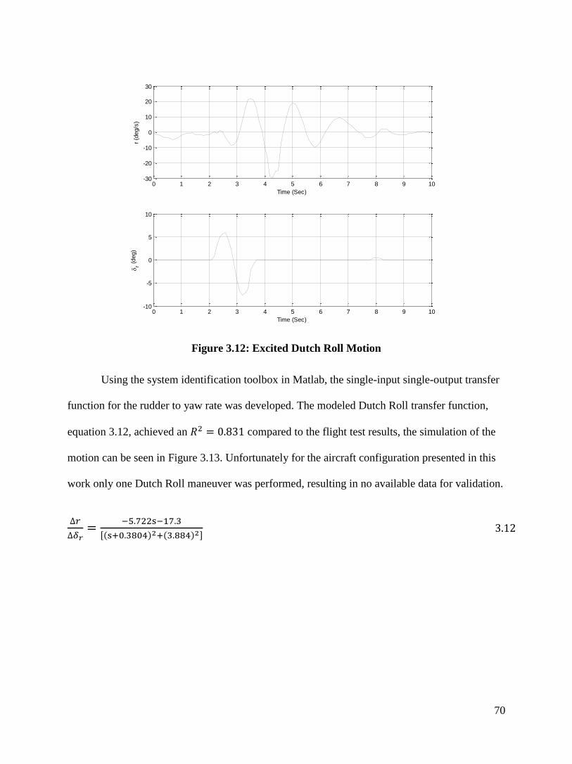
70
Figure 3.12: Excited Dutch Roll Motion
Using the system identification toolbox in Matlab, the single-input single-output transfer
function for the rudder to yaw rate was developed. The modeled Dutch Roll transfer function,
equation 3.12, achieved an compared to the flight test results, the simulation of the
motion can be seen in Figure 3.13. Unfortunately for the aircraft configuration presented in this
work only one Dutch Roll maneuver was performed, resulting in no available data for validation.
[( ) ( ) ] 3.12
0 1 2 3 4 5 6 7 8 9 10-30
-20
-10
0
10
20
30
Time (Sec)
r (d
eg/s
)
0 1 2 3 4 5 6 7 8 9 10-10
-5
0
5
10
Time (Sec)
r (
deg)
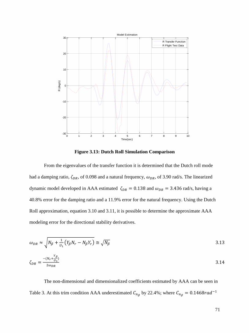
71
Figure 3.13: Dutch Roll Simulation Comparison
From the eigenvalues of the transfer function it is determined that the Dutch roll mode
had a damping ratio, , of 0.098 and a natural frequency, , of 3.90 rad/s. The linearized
dynamic model developed in AAA estimated and rad/s, having a
40.8% error for the damping ratio and a 11.9% error for the natural frequency. Using the Dutch
Roll approximation, equation 3.10 and 3.11, it is possible to determine the approximate AAA
modeling error for the directional stability derivatives.
√
( ) √ 3.13
(
)
3.14
The non-dimensional and dimensionalized coefficients estimated by AAA can be seen in
Table 3. At this trim condition AAA underestimated by 22.4%; where
0 1 2 3 4 5 6 7 8 9 10-30
-20
-10
0
10
20
30Model Estimation
Time(sec)
R (
deg/s
)
R Transfer Function
R Flight Test Data

72
satisfies the actual natural frequency of the excited Dutch roll mode. With this correction
applied and
would have a combined overestimated error of 30.3%, according to the
reduced order Dutch Roll approximation. However, it is inconclusive if the damping error is due
to incorrect and
estimations as high roll rates and slipstream interference were
experienced in flight, and could reduce the directional damping. These results indicate that AAA
is capable of adequately modeling directional derivatives despite the complexities of the V-tail,
as the dynamic mode error could potentially be caused by the off-trim flight condition and
slipstream interference.
Table 3: Linearized Approximations of Dutch Roll Stability
0.1108 11.1345
-0.1331 -0.8479
-0.4180 -32.0454
0.2865 1.3917
3.4 Rudder Doublet Conclusions
The effects of the brief rudder doublet have shed light on many characteristics of the
Meridian UAS which could lead to catastrophic events for an untrained pilot and aid in future
development of dynamic models used for flight controllers. It was shown that high frequency
control inputs can lead to PIO, resulting in undesirable effects such as uncommanded and
undamped angular rates as well as the retarding of commanded moments due to unsteady vortex
interaction at the tail. Most importantly high yaw rates should be avoided as this can lead to a
loss of lift. High rates are also factors in developing unsteady aerodynamics, and with the strong
coupling between all three axes, this has potential to drive the aircraft unstable due to unsteady
vortex interaction.
73
It has been shown that AAA is an adequate tool for determining directional dynamic
stability for a UAS from the system identification performed. However, the stability and control
derivatives have been shown to be highly transient throughout flight, primarily dependent on the
reduced frequency, angular rates, and airflow angles. It is recommended that thorough CFD
analyses be performed for a three-dimensional aircraft to determine the airflow effects at the V-
tail due to the downstream vortex wakes generated by trailing edge vortices and flow separation
over the fuselage. Further CFD analyses should be performed to determine effects due to vortex
interaction between each ruddervator surface at varying ruddervator deflections and airflow
angles. The downwash from one ruddervator surface may drastically affect the lift distribution on
the other surface, leading to unstable or undamped yawing and pitching motions.
As mentioned, hinge-moment analysis should be performed for the ruddervator control
surfaces as they are capable of experiencing high aerodynamic loads in flight. Due to only one
servo per ruddervator, an actuator failure in flight would most likely result in a loss of aircraft
due to the high coupling effects and reduced control effectiveness. It is recommended that
control state feedback be implemented to determine how the control services react to the
commanded values; this may also identify the presence of flutter. Finally air data probes should
be installed at the mean geometric chord of each ruddervator surface to determine local airspeed,
angle of attack, and sideslip angle, as all values used in this analysis are estimates with low
confidence of the true airflow angles at the tail.
74
4 Elevator Doublet Analysis
During the first NEEM flight an elevator doublet was performed to assess the
longitudinal stability and damping of the aircraft. As with the rudder doublet, this motion reveals
some cross-coupling motions due to the V-tail configuration, as well as aircraft performance
during a high frequency, large amplitude, and oscillatory pitching motion. Preceding the elevator
doublet, controlled aircraft maneuvers were made in attempt to trim the aircraft and return all
control surfaces to a neutral position, to reduce the motion not induced by elevator deflections.
Firstly, results will be presented which discuss the effects of returning control surfaces to neutral
positions followed by a comparison of the flight test results to the linearized dynamic model.
4.1 Elevator Deflection and Throttle Reduction
In preparation for the elevator doublet, the throttle position was reduced from 80% to
70%, five seconds prior to returning all controls to neutral positions; this is not shown in the
data, but necessary to mention, as the aircraft was initially gaining altitude and airspeed. As
previously discussed, the neutral elevator position was not properly trimmed, which resulted in α
reducing from 3.2° to -2.5° during the first second neutral control flight. The decreasing angle of
attack resulted in a loss of lift, with the minimum lift, , occruing at t = 0.9 seconds,
with a normal wing loading, , of 0.405g’s. The loss of lift resulting from untrimmed flight can
be seen in Figure 4.1.

75
Figure 4.1: Untrimmed Loss of Lift
The natural tendency of all stable aircraft is to reach an equilibrium state over time. A
change in elevator deflection and throttle position can induce the phugoid mode, or long period,
which is characterized by a periodic gain and dispersion of energy at a low frequency. An
aperiodic gain in longitudinal energy was experienced by the Meridian, with becoming
negative and becoming positive, as the aircraft remained untrimmed. At t = 0.9 seconds,
when the aircraft reached a minimum lift, gained energy, followed by
gaining
energy at t = 1.0 seconds. Although the aircraft would eventually reach a trim state, the time to
do so would result in the aircraft going beyond the external pilot’s LOS. In an additional attempt
to trim the aircraft, the pilot further reduced the throttle position from 70% to 66%, at t = 1.1
seconds, which dissipated the longitudinal energy generated by the aircraft. The changes in
longitudinal energy between t = 0 seconds and t = 3 seconds can be seen in Figure 4.2.
0 0.2 0.4 0.6 0.8 1 1.2 1.4 1.6 1.8 28760
8770
8780
Time (sec)
Altitude A
MS
L (
ft)
0 0.2 0.4 0.6 0.8 1 1.2 1.4 1.6 1.8 2200
210
220
Time (sec)
TA
S (
kts
)
0 0.2 0.4 0.6 0.8 1 1.2 1.4 1.6 1.8 20
0.5
1
Time (sec)
CZ
0 0.2 0.4 0.6 0.8 1 1.2 1.4 1.6 1.8 2-5
0
5
Time (sec)
(
deg)

76
Figure 4.2: Longitudinal Gain and Dissipation of Energy During Response to Control
Commands
After the pilot reduced the throttle position he attempted to bring the pitch angle to zero
through a series of elevator deflections. However, the data continued to show the pitch angle to
be insensitive to elevator commands, and since compatibility analysis was performed prior to
processing the data it was originally assumed that this occurrence could be explained as a slow
response to control inputs. Further analysis was performed, which indicates that the autopilot
EKF does not accurately estimate the pitch angle during high frequency pitch rates. A series of
tests were performed to identify and validate the inaccurate estimates, which will be described in
detail in the following text.
As a preliminary test to validate the attitude angles estimated by the autopilot, the raw
angular rates measured by autopilot rate gyro sensors were used to simulate the attitude angles
using the rotational kinematic equations of motion. This test was performed to see if the autopilot
estimates could be replicated using the same signals and angle initial conditions. Also no
0 0.5 1 1.5 2 2.5 3
4
5
6
Time (sec)
e (
deg)
0 0.5 1 1.5 2 2.5 360
65
70
Time (sec)
t (
%)
0 0.5 1 1.5 2 2.5 3
-60
-40
-20
0
20
Time (sec)
Cm
q(o
sc)
0 0.5 1 1.5 2 2.5 3
0
100
200
Time (sec)
CZ
q(o
sc)

77
filtering or bias removal was performed prior to performing the simulations; the kinematic
equations were simply solved as a series of ordinary differential equations using the raw angular
rate data. As such, the simulations produced results very near to the autopilot estimates for and
ψ, with respective values of 0.936 and 0.990, however there was no correlation in θ, shown in
Figure 4.3
Figure 4.3: State Estimation Discrepancies Between Autopilot and IMU
To further validate the discrepancy in the autopilot EKF, data from an auxiliary inertial
measurement unit (IMU) was compared against for the same time interval. The IMU EKF
estimates matched the simulation data well, even with initial conditions coming from the
autopilot estimations. Again there was no correlation between the autopilot pitch angle and the
IMU pitch angle, but there was roughly a bias between the heading angle estimated by the
autopilot and IMU. It is difficult to quantify the accuracy of either heading estimate though, as
the autopilot did not have a magnetometer in the loop to serve as a reference, but rather relied on
0 1 2 3 4 5 6-10
-5
0
5
10
Time (sec)
(
deg)
Simulation
Autopilot EKF
IMU EKF
0 1 2 3 4 5 6
-10
-5
0
5
Time (sec)
(
deg)
0 1 2 3 4 5 6170
180
190
200
Time (sec)
(
deg)
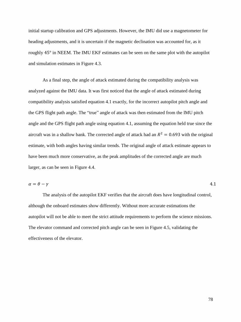
78
initial startup calibration and GPS adjustments. However, the IMU did use a magnetometer for
heading adjustments, and it is uncertain if the magnetic declination was accounted for, as it
roughly in NEEM. The IMU EKF estimates can be seen on the same plot with the autopilot
and simulation estimates in Figure 4.3.
As a final step, the angle of attack estimated during the compatibility analysis was
analyzed against the IMU data. It was first noticed that the angle of attack estimated during
compatibility analysis satisfied equation 4.1 exactly, for the incorrect autopilot pitch angle and
the GPS flight path angle. The “true” angle of attack was then estimated from the IMU pitch
angle and the GPS flight path angle using equation 4.1, assuming the equation held true since the
aircraft was in a shallow bank. The corrected angle of attack had an with the original
estimate, with both angles having similar trends. The original angle of attack estimate appears to
have been much more conservative, as the peak amplitudes of the corrected angle are much
larger, as can be seen in Figure 4.4.
4.1
The analysis of the autopilot EKF verifies that the aircraft does have longitudinal control,
although the onboard estimates show differently. Without more accurate estimations the
autopilot will not be able to meet the strict attitude requirements to perform the science missions.
The elevator command and corrected pitch angle can be seen in Figure 4.5, validating the
effectiveness of the elevator.
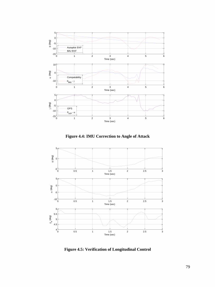
79
Figure 4.4: IMU Correction to Angle of Attack
Figure 4.5: Verification of Longitudinal Control
0 1 2 3 4 5 6-15
-10
-5
0
5
Time (sec)
(
deg)
Autopilot EKF
IMU EKF
0 1 2 3 4 5 6
-10
0
10
Time (sec)
(
deg)
Compatability
IMU
-
0 1 2 3 4 5 6-15
-10
-5
0
5
Time (sec)
(d
eg)
GPS
A/P
-
0 0.5 1 1.5 2 2.5 3-5
0
5
Time (sec)
(
deg)
0 0.5 1 1.5 2 2.5 3-10
-5
0
5
Time (sec)
(
deg)
0 0.5 1 1.5 2 2.5 34
4.5
5
5.5
6
Time (sec)
e (
deg)
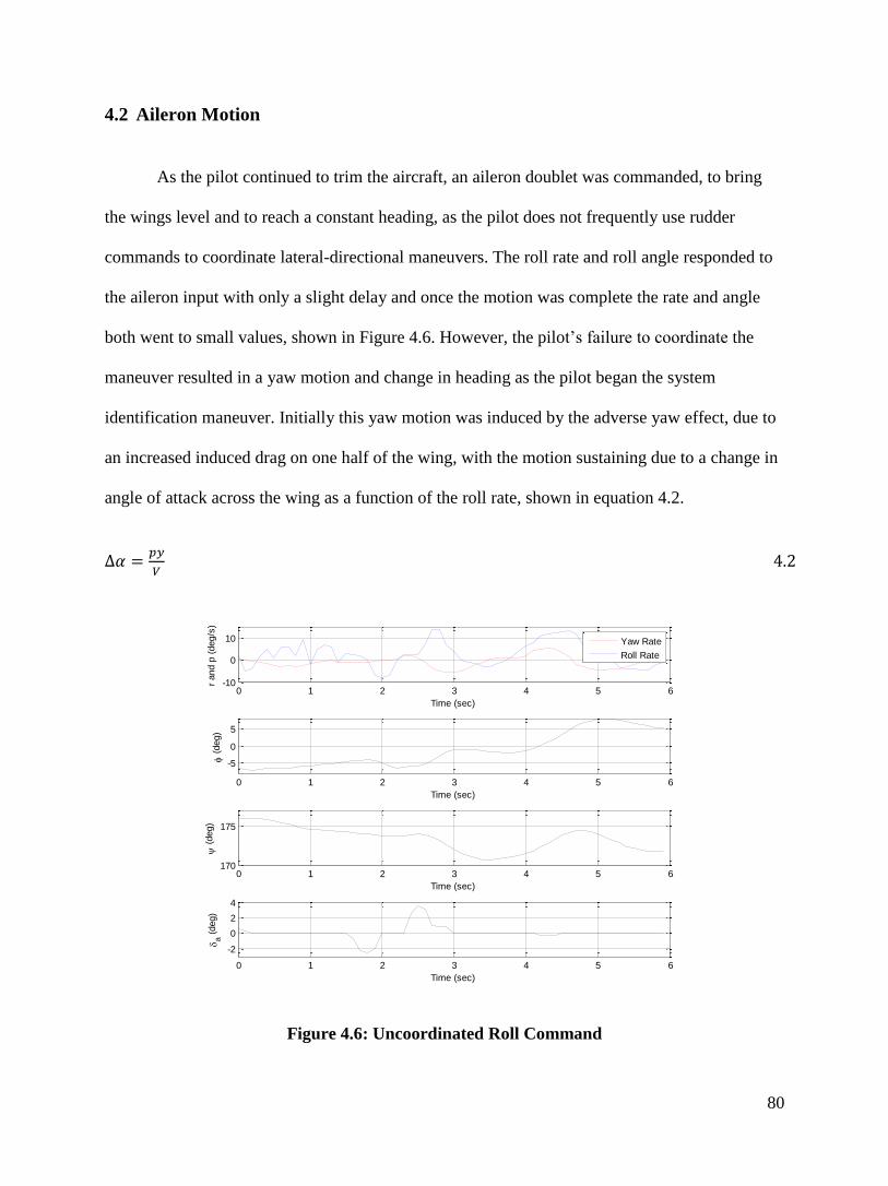
80
4.2 Aileron Motion
As the pilot continued to trim the aircraft, an aileron doublet was commanded, to bring
the wings level and to reach a constant heading, as the pilot does not frequently use rudder
commands to coordinate lateral-directional maneuvers. The roll rate and roll angle responded to
the aileron input with only a slight delay and once the motion was complete the rate and angle
both went to small values, shown in Figure 4.6. However, the pilot’s failure to coordinate the
maneuver resulted in a yaw motion and change in heading as the pilot began the system
identification maneuver. Initially this yaw motion was induced by the adverse yaw effect, due to
an increased induced drag on one half of the wing, with the motion sustaining due to a change in
angle of attack across the wing as a function of the roll rate, shown in equation 4.2.
4.2
Figure 4.6: Uncoordinated Roll Command
0 1 2 3 4 5 6-10
0
10
Time (sec)
r and p
(deg/s
)
Yaw Rate
Roll Rate
0 1 2 3 4 5 6
-5
0
5
Time (sec)
(
deg)
0 1 2 3 4 5 6170
175
Time (sec)
(
deg)
0 1 2 3 4 5 6
-2
0
2
4
Time (sec)
a (
deg)
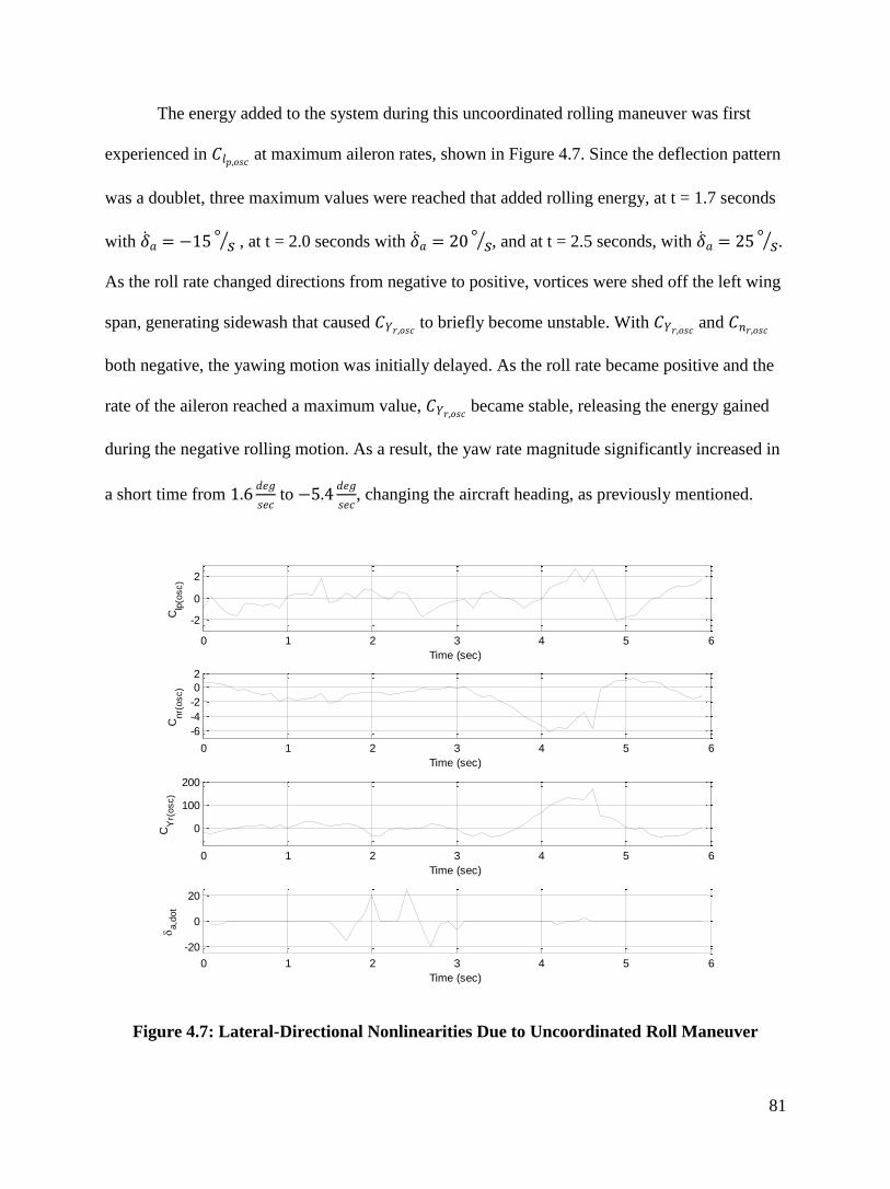
81
The energy added to the system during this uncoordinated rolling maneuver was first
experienced in at maximum aileron rates, shown in Figure 4.7. Since the deflection pattern
was a doublet, three maximum values were reached that added rolling energy, at t = 1.7 seconds
with ⁄ , at t = 2.0 seconds with
⁄ , and at t = 2.5 seconds, with ⁄ .
As the roll rate changed directions from negative to positive, vortices were shed off the left wing
span, generating sidewash that caused to briefly become unstable. With
and
both negative, the yawing motion was initially delayed. As the roll rate became positive and the
rate of the aileron reached a maximum value, became stable, releasing the energy gained
during the negative rolling motion. As a result, the yaw rate magnitude significantly increased in
a short time from
to
, changing the aircraft heading, as previously mentioned.
Figure 4.7: Lateral-Directional Nonlinearities Due to Uncoordinated Roll Maneuver
0 1 2 3 4 5 6
-2
0
2
Time (sec)
Clp
(osc)
0 1 2 3 4 5 6
-6
-4
-2
0
2
Time (sec)
Cnr(
osc)
0 1 2 3 4 5 6
0
100
200
Time (sec)
CY
r(osc)
0 1 2 3 4 5 6
-20
0
20
Time (sec)
a,d
ot
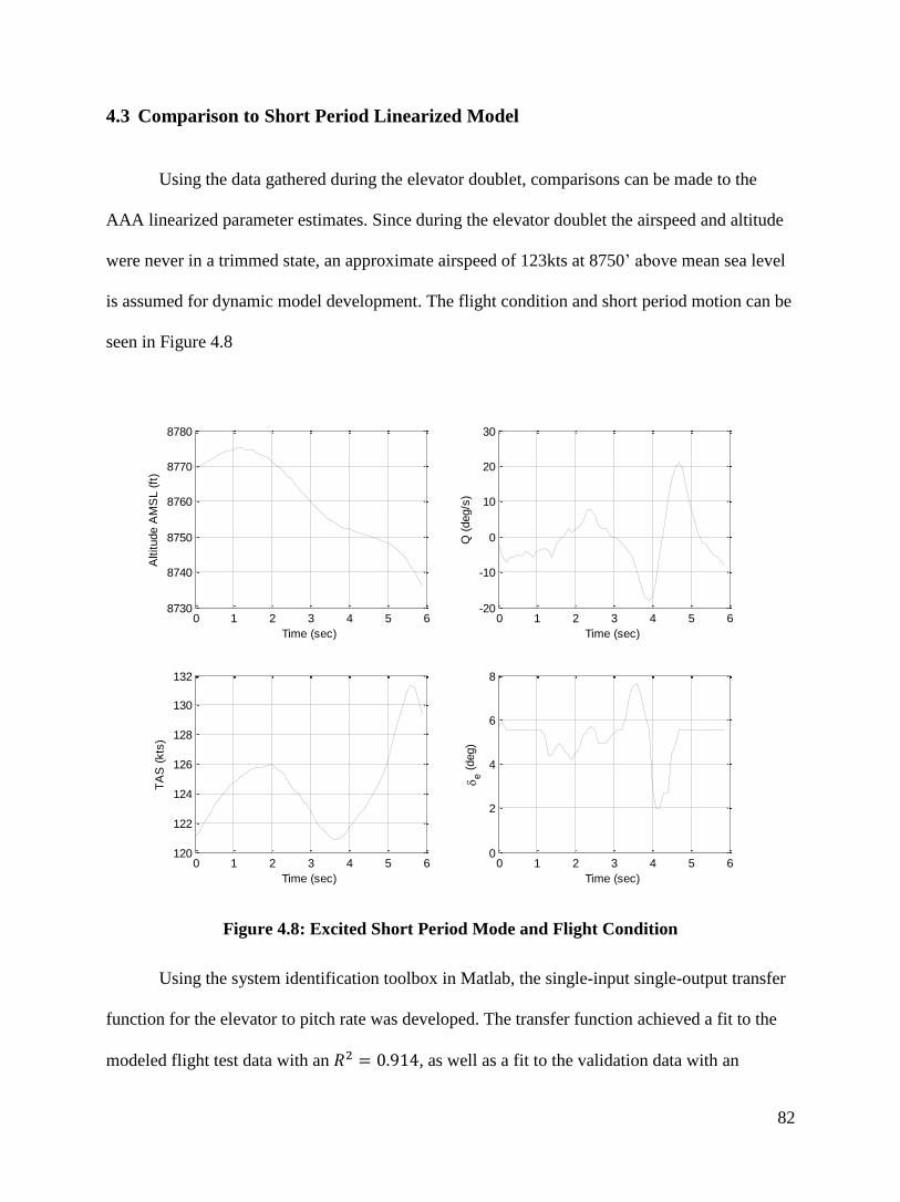
82
4.3 Comparison to Short Period Linearized Model
Using the data gathered during the elevator doublet, comparisons can be made to the
AAA linearized parameter estimates. Since during the elevator doublet the airspeed and altitude
were never in a trimmed state, an approximate airspeed of 123kts at 8750’ above mean sea level
is assumed for dynamic model development. The flight condition and short period motion can be
seen in Figure 4.8
Figure 4.8: Excited Short Period Mode and Flight Condition
Using the system identification toolbox in Matlab, the single-input single-output transfer
function for the elevator to pitch rate was developed. The transfer function achieved a fit to the
modeled flight test data with an , as well as a fit to the validation data with an
0 1 2 3 4 5 68730
8740
8750
8760
8770
8780
Time (sec)
Altitude A
MS
L (
ft)
0 1 2 3 4 5 6-20
-10
0
10
20
30
Time (sec)
Q (
deg/s
)
0 1 2 3 4 5 6120
122
124
126
128
130
132
Time (sec)
TA
S (
kts
)
0 1 2 3 4 5 60
2
4
6
8
Time (sec)
e (
deg)
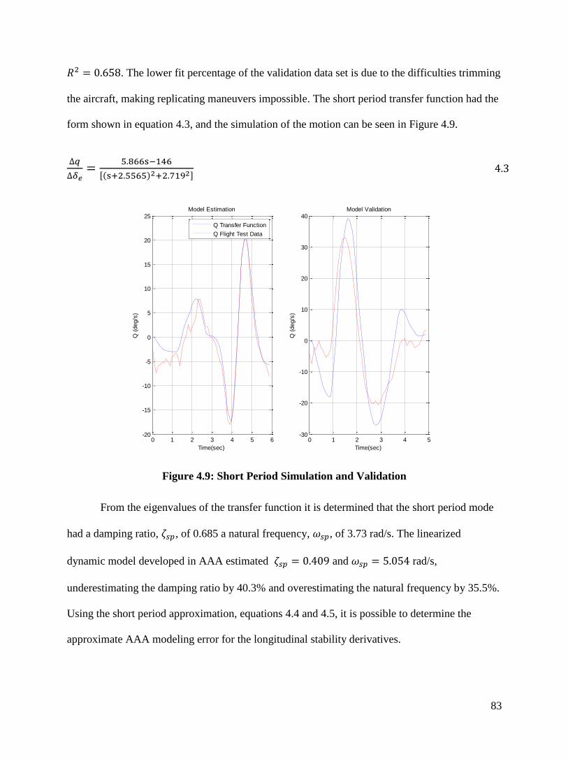
83
. The lower fit percentage of the validation data set is due to the difficulties trimming
the aircraft, making replicating maneuvers impossible. The short period transfer function had the
form shown in equation 4.3, and the simulation of the motion can be seen in Figure 4.9.
[( ) ] 4.3
Figure 4.9: Short Period Simulation and Validation
From the eigenvalues of the transfer function it is determined that the short period mode
had a damping ratio, , of 0.685 a natural frequency, , of 3.73 rad/s. The linearized
dynamic model developed in AAA estimated and rad/s,
underestimating the damping ratio by 40.3% and overestimating the natural frequency by 35.5%.
Using the short period approximation, equations 4.4 and 4.5, it is possible to determine the
approximate AAA modeling error for the longitudinal stability derivatives.
0 1 2 3 4 5 6-20
-15
-10
-5
0
5
10
15
20
25Model Estimation
Time(sec)
Q (
deg/s
)
0 1 2 3 4 5-30
-20
-10
0
10
20
30
40Model Validation
Time(sec)
Q (
deg/s
)
Q Transfer Function
Q Flight Test Data
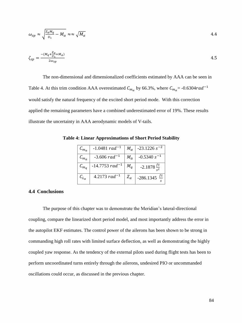
84
√
√ 4.4
(
)
4.5
The non-dimensional and dimensionalized coefficients estimated by AAA can be seen in
Table 4. At this trim condition AAA overestimated by 66.3%, where
= -0.6304
would satisfy the natural frequency of the excited short period mode. With this correction
applied the remaining parameters have a combined underestimated error of 19%. These results
illustrate the uncertainty in AAA aerodynamic models of V-tails.
Table 4: Linear Approximations of Short Period Stability
-1.0481 -23.1226
-3.606 -0.5340
-14.7753 -2.1878
4.2173 -286.1345
4.4 Conclusions
The purpose of this chapter was to demonstrate the Meridian’s lateral-directional
coupling, compare the linearized short period model, and most importantly address the error in
the autopilot EKF estimates. The control power of the ailerons has been shown to be strong in
commanding high roll rates with limited surface deflection, as well as demonstrating the highly
coupled yaw response. As the tendency of the external pilots used during flight tests has been to
perform uncoordinated turns entirely through the ailerons, undesired PIO or uncommanded
oscillations could occur, as discussed in the previous chapter.
85
The effects of the brief elevator doublet have indicated the level of uncertainty resulting
from AAA analysis for this flight configuration. The linearized model has shown to
underestimate the damping ratio by 40.3% and overestimate the natural frequency by 35.5%,
when compared to actual excited motion. The error in the natural frequency estimated by the
linearized model is most likely due to the V-tail being modeled as a horizontal projection of the
surface with a constant downwash across the surface, making the effectiveness much greater than
it is in actuality. The estimated damping ratio error is more difficult to quantify as the effects due
to the slipstream, ski configuration, downwash angle, and angle of attack rate are not known.
Finally the autopilot EKF used for attitude determination has shown to inaccurately
estimate the pitch angle. This error does not originate from inaccurate sensor measurements
though, as simulations using the onboard sensors have independently been validated against
estimations from an auxiliary IMU. Corrections to the EKF should be addressed prior to future
flights, as the response time of the autopilot may be inadequate during high pitch rates.
Furthermore, the autopilot heading estimation should be tested both with and without a
magnetometer in the loop, to determine if the system accurately performs without using
magnetometer measurements as a reference, or if there is accumulated estimation error over
time.
86
5 Unpowered Flight and Mode Transition Analysis
The second flight of the Meridian in NEEM Greenland was unique, as the autopilot
experienced a microsecond glitch that commanded the engine to shut down. Through this
unplanned system malfunction, unpowered flight test data was collected that illustrates the
aerodynamic performance of the aircraft without the presence of the slipstream. During this
flight several commanded and uncommanded transitions between the piloted RC mode, the
assisted mode (referred to herein as Manual mode), and the autonomous Home mode occurred.
The Home mode is an autonomous mode which commands the aircraft to hold a commanded
altitude and airspeed, at a given radius, about a defined point in space for a given latitude,
longitude, and altitude above sea level.
The first transitions from RC mode to Manual mode, Manual mode to Home mode, and
the return to RC mode were all commanded via the RC pilot 72MHz or ground station 900MHz
communication links. The Home mode was only engaged briefly due to the high angular rates
and large control surface oscillations, commanded by the flight controller. The other portions of
flight where the aircraft enters Manual mode and returns to RC mode were all uncommanded
events due to a loss, and eventual recovery, of the 72MHz communication link. These Manual
mode transitions serve as a failsafe setting in the event of a communication loss, with the aircraft
being commanded to hold the current course with the wings level. The glitch in the autopilot
occurred between the two uncommanded communication losses, forcing the pilot to make an
emergency unpowered landing. This chapter will begin with the discussion of the flight mode
transitions, followed by an analysis of the unpowered landing and conclusions.
Unfortunately independent data sets were not available to compare against for this flight,
therefore an Extended Kalman Filter was constructed so to further evaluate the estimated attitude
angles. The prediction functions used in the EKF were a discretized form of the rotational
87
kinematic equations of motion, with the measured angular rates serving as the inputs to the
system, as shown in equation 5.1. Since the attitude angles are measured with respect to the
inertial frame, the GPS velocities served as the observation states, with the body accelerations
being transformed through an orthonormal transformation from the body frame to inertial frame
as a function of the attitude angles, shown in equation 5.2. As one of the advantages of using an
EFK is the stochastic estimations, determining the variances of the accelerometers, rate gyros,
GPS velocities, as well as for the initial attitude estimation was essential [56]. The variances
were calculated from Meridian ground test data where the aircraft was undisturbed, allowing for
the best case in capturing the sensor uncertainty over a long portion of time.
[
] [
] [
] [ ] [
( )
( )
( )] 5.1
[
] ( ( ) [
] [ ]) [
( )
( )
( )
] [
( )
( )
( )] 5.2
The developed EKF estimated the attitude angles during the 2nd
NEEM flight using raw
data from the autopilot, to allow for comparisons to be made between the two estimations. Since
sensor variance determination was performed using old ground test data, with no real value, it is
surprising how similar the estimates are, shown in Figure 5.1. The largest and most frequent
estimation bias was seen in the pitch angle, specifically for ; however, the pitch angle
estimate from the FLM compatibility analysis showed no correlation to the two EFK estimates.
Although the two EFK estimates are similar, it does not necessarily add confidence to the data,
as the autopilot has been in use for five years and the data used in determining the variances was
from 2009. The two filters were designed using sensor data from the same time period, and the
current performance level of the sensors is unknown. More data is necessary to accurately
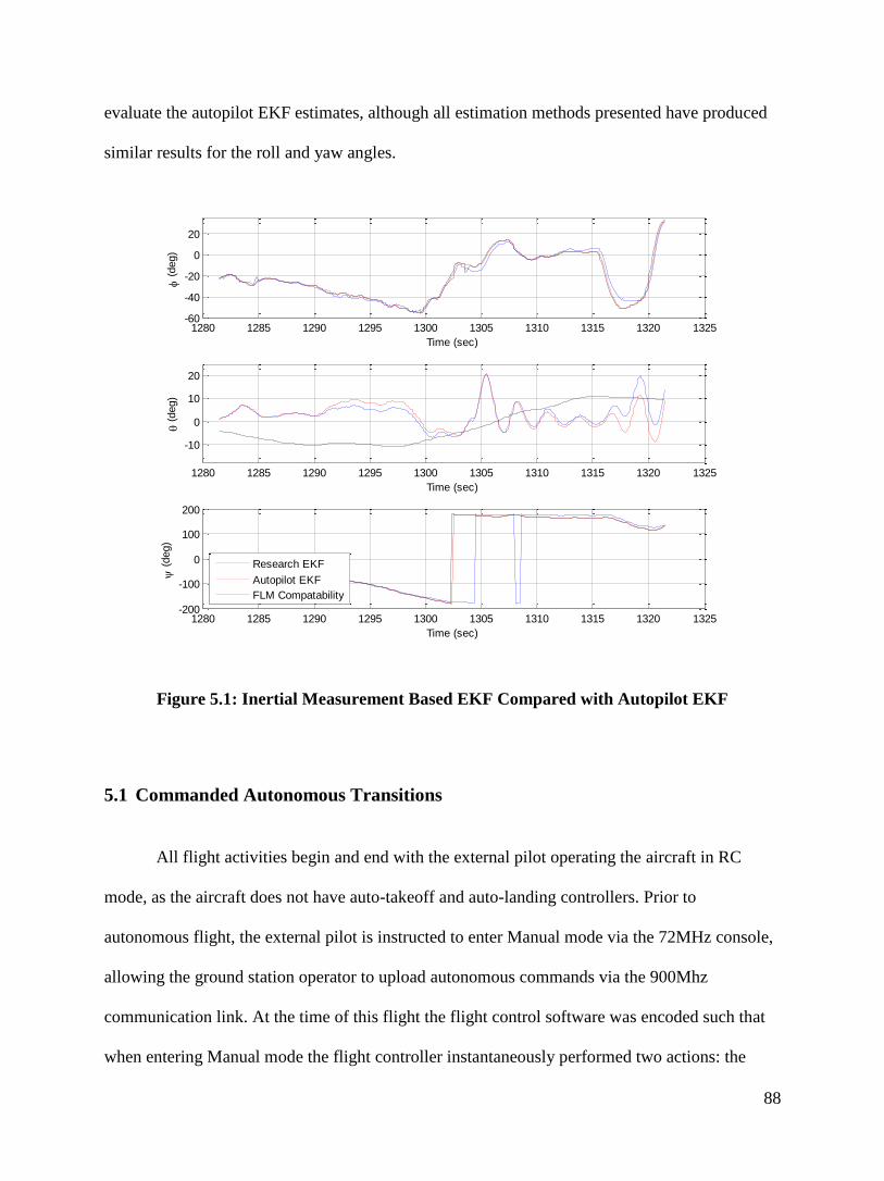
88
evaluate the autopilot EKF estimates, although all estimation methods presented have produced
similar results for the roll and yaw angles.
Figure 5.1: Inertial Measurement Based EKF Compared with Autopilot EKF
5.1 Commanded Autonomous Transitions
All flight activities begin and end with the external pilot operating the aircraft in RC
mode, as the aircraft does not have auto-takeoff and auto-landing controllers. Prior to
autonomous flight, the external pilot is instructed to enter Manual mode via the 72MHz console,
allowing the ground station operator to upload autonomous commands via the 900Mhz
communication link. At the time of this flight the flight control software was encoded such that
when entering Manual mode the flight controller instantaneously performed two actions: the
1280 1285 1290 1295 1300 1305 1310 1315 1320 1325-60
-40
-20
0
20
(
deg)
Time (sec)
1280 1285 1290 1295 1300 1305 1310 1315 1320 1325
-10
0
10
20
(
deg)
Time (sec)
1280 1285 1290 1295 1300 1305 1310 1315 1320 1325-200
-100
0
100
200
(
deg)
Time (sec)
Research EKF
Autopilot EKF
FLM Compatability
89
elevator deflection is commanded to and the ailerons are commanded to level the wings,
without any rate or deflection limiters. These commands have led to high angular rates and large
variations in the airflow angles, which result in nonlinear and unsteady aerodynamic effects.
These flights in NEEM were the last to use such failsafe logic, the current failsafe settings retain
the elevator command at the time of transition; however, the wing level command is still present.
As well as having the autonomous failsafe, there is also the operational failsafe that allows the
pilot to regain command of the aircraft at any point in flight, though this transition
instantaneously transfers control to the current stick placement on the pilot console.
The first mode transition to be discussed occurred at t = 64.0 seconds, with the autopilot
autonomously commanding substantial aileron deflection and bringing the elevator deflection to
, shown in Figure 5.2. As the transition began, the angle of attack was at , but rapidly
increased to at t = 65.4 seconds. During the maximum pitch rate, from t = 64.3 seconds to
t= 65.4 seconds, and
were both unstable with the yaw rate changing directions
multiple times, shown in Figure 5.3 and Figure 5.4.
During the time segment when the oscillatory yaw damping derivatives are unstable, the
aileron deflection and roll rate are positive, which should create a negative yaw rate due the
higher induced drag on the left wing surface. However, at t = 64.9 seconds the yaw rate changes
from negative to positive and the roll rate becomes increasingly positive. The change in yaw rate
direction as the V-tail was near the downstream vortices shedding off the right wing, which
generates negative sidewash, due to up-deflected right aileron [39]. The increased roll rate can be
explained in part by the same side wash effect, but is a contributing factor. High
angles of attack are a cause for the stability axis moment arm to change signs, which
introduces a destabilizing rolling moment due to the large negative moment arm [18]. Figure 5.5
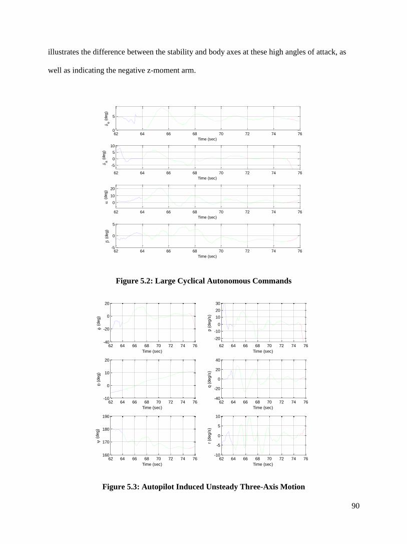
90
illustrates the difference between the stability and body axes at these high angles of attack, as
well as indicating the negative z-moment arm.
Figure 5.2: Large Cyclical Autonomous Commands
Figure 5.3: Autopilot Induced Unsteady Three-Axis Motion
62 64 66 68 70 72 74 760
5
Time (sec)
e (
deg)
62 64 66 68 70 72 74 76
-5
0
5
10
Time (sec)
a (
deg)
62 64 66 68 70 72 74 76
0
10
20
Time (sec)
(
deg)
62 64 66 68 70 72 74 76-5
0
5
Time (sec)
(
deg)
62 64 66 68 70 72 74 76-40
-20
0
20
Time (sec)
(
deg)
62 64 66 68 70 72 74 76
-20
-10
0
10
20
30
Time (sec)
p (
deg/s
)
62 64 66 68 70 72 74 76-10
0
10
20
Time (sec)
(
deg)
62 64 66 68 70 72 74 76-40
-20
0
20
40
Time (sec)
q (
deg/s
)
62 64 66 68 70 72 74 76160
170
180
190
Time (sec)
(
deg)
62 64 66 68 70 72 74 76-10
-5
0
5
10
Time (sec)
r (d
eg/s
)
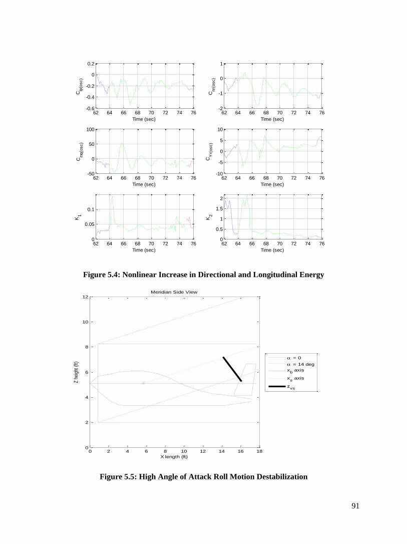
91
Figure 5.4: Nonlinear Increase in Directional and Longitudinal Energy
Figure 5.5: High Angle of Attack Roll Motion Destabilization
62 64 66 68 70 72 74 76-0.6
-0.4
-0.2
0
0.2
Time (sec)
Clp
(osc)
62 64 66 68 70 72 74 76-2
-1
0
1
Time (sec)
Cnr(
osc)
62 64 66 68 70 72 74 76-50
0
50
100
Time (sec)
Cm
q(o
sc)
62 64 66 68 70 72 74 76-10
-5
0
5
10
Time (sec)
CY
r(osc)
62 64 66 68 70 72 74 760
0.05
0.1
Time (sec)
K1
62 64 66 68 70 72 74 760
0.5
1
1.5
2
Time (sec)
K2
0 2 4 6 8 10 12 14 16 180
2
4
6
8
10
12
X length (ft)
Z he
ight
(ft)
Meridian Side View
= 0
= 14 deg
xb axis
xs axis
zvs
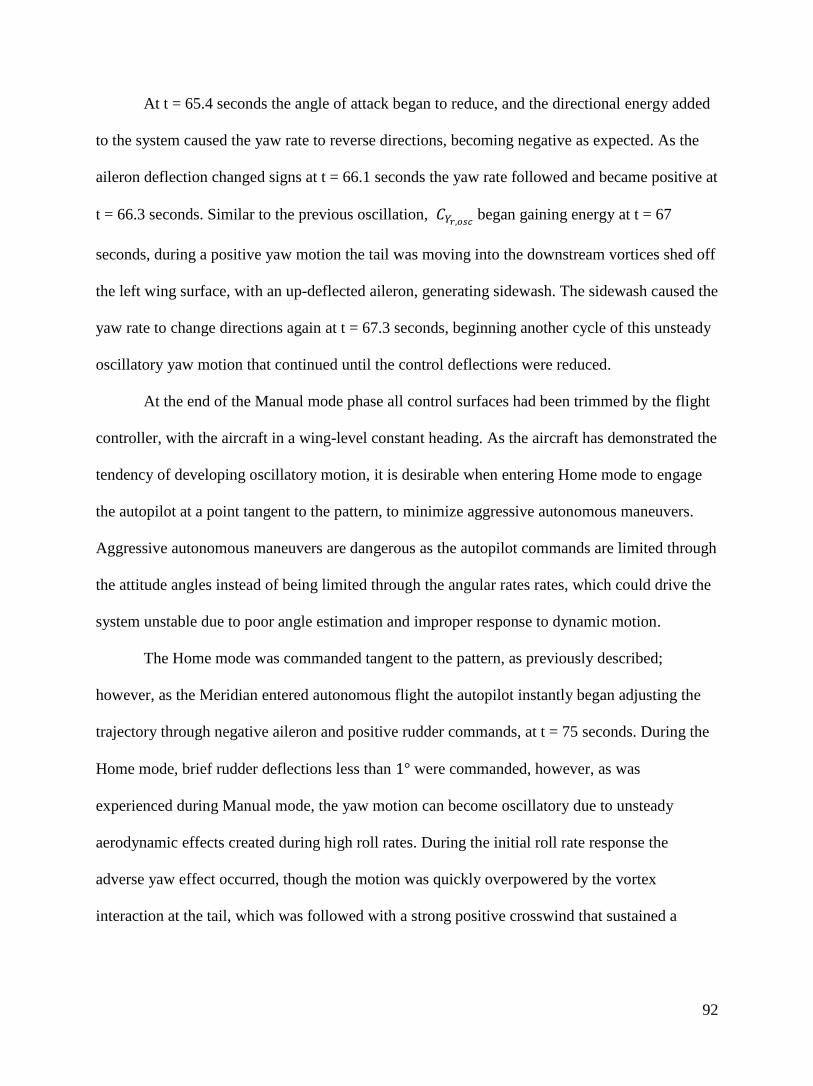
92
At t = 65.4 seconds the angle of attack began to reduce, and the directional energy added
to the system caused the yaw rate to reverse directions, becoming negative as expected. As the
aileron deflection changed signs at t = 66.1 seconds the yaw rate followed and became positive at
t = 66.3 seconds. Similar to the previous oscillation, began gaining energy at t = 67
seconds, during a positive yaw motion the tail was moving into the downstream vortices shed off
the left wing surface, with an up-deflected aileron, generating sidewash. The sidewash caused the
yaw rate to change directions again at t = 67.3 seconds, beginning another cycle of this unsteady
oscillatory yaw motion that continued until the control deflections were reduced.
At the end of the Manual mode phase all control surfaces had been trimmed by the flight
controller, with the aircraft in a wing-level constant heading. As the aircraft has demonstrated the
tendency of developing oscillatory motion, it is desirable when entering Home mode to engage
the autopilot at a point tangent to the pattern, to minimize aggressive autonomous maneuvers.
Aggressive autonomous maneuvers are dangerous as the autopilot commands are limited through
the attitude angles instead of being limited through the angular rates rates, which could drive the
system unstable due to poor angle estimation and improper response to dynamic motion.
The Home mode was commanded tangent to the pattern, as previously described;
however, as the Meridian entered autonomous flight the autopilot instantly began adjusting the
trajectory through negative aileron and positive rudder commands, at t = 75 seconds. During the
Home mode, brief rudder deflections less than were commanded, however, as was
experienced during Manual mode, the yaw motion can become oscillatory due to unsteady
aerodynamic effects created during high roll rates. During the initial roll rate response the
adverse yaw effect occurred, though the motion was quickly overpowered by the vortex
interaction at the tail, which was followed with a strong positive crosswind that sustained a
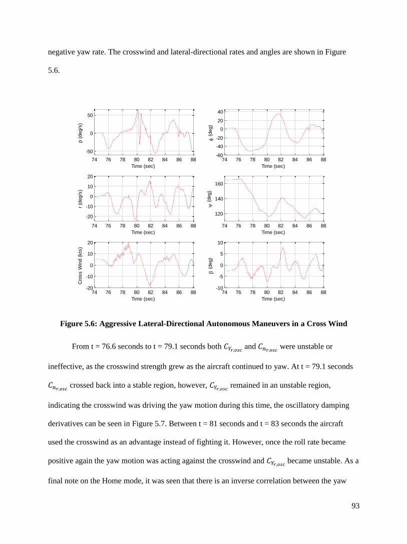
93
negative yaw rate. The crosswind and lateral-directional rates and angles are shown in Figure
5.6.
Figure 5.6: Aggressive Lateral-Directional Autonomous Maneuvers in a Cross Wind
From t = 76.6 seconds to t = 79.1 seconds both and
were unstable or
ineffective, as the crosswind strength grew as the aircraft continued to yaw. At t = 79.1 seconds
crossed back into a stable region, however,
remained in an unstable region,
indicating the crosswind was driving the yaw motion during this time, the oscillatory damping
derivatives can be seen in Figure 5.7. Between t = 81 seconds and t = 83 seconds the aircraft
used the crosswind as an advantage instead of fighting it. However, once the roll rate became
positive again the yaw motion was acting against the crosswind and became unstable. As a
final note on the Home mode, it was seen that there is an inverse correlation between the yaw
74 76 78 80 82 84 86 88
-50
0
50
Time (sec)
p (
deg/s
)
74 76 78 80 82 84 86 88-60
-40
-20
0
20
40
Time (sec)
(
deg)
74 76 78 80 82 84 86 88
-20
-10
0
10
20
Time (sec)
r (d
eg/s
)
74 76 78 80 82 84 86 88
120
140
160
Time (sec)
(
deg)
74 76 78 80 82 84 86 88-20
-10
0
10
20
Time (sec)
Cro
ss W
ind (
kts
)
74 76 78 80 82 84 86 88-10
-5
0
5
10
Time (sec)
(
deg)
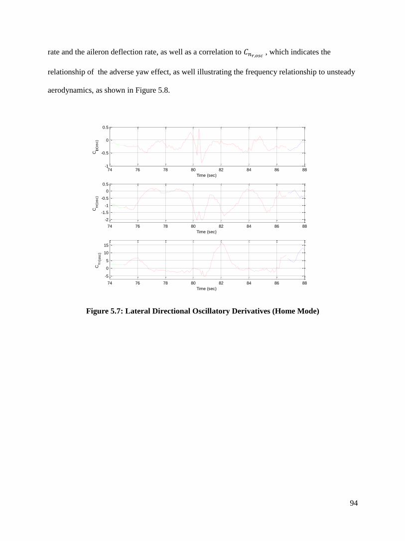
94
rate and the aileron deflection rate, as well as a correlation to , which indicates the
relationship of the adverse yaw effect, as well illustrating the frequency relationship to unsteady
aerodynamics, as shown in Figure 5.8.
Figure 5.7: Lateral Directional Oscillatory Derivatives (Home Mode)
74 76 78 80 82 84 86 88-1
-0.5
0
0.5
Time (sec)
Clp
(osc)
74 76 78 80 82 84 86 88
-2
-1.5
-1
-0.5
0
0.5
Time (sec)
Cnr(
osc)
74 76 78 80 82 84 86 88
-5
0
5
10
15
Time (sec)
CY
r(osc)
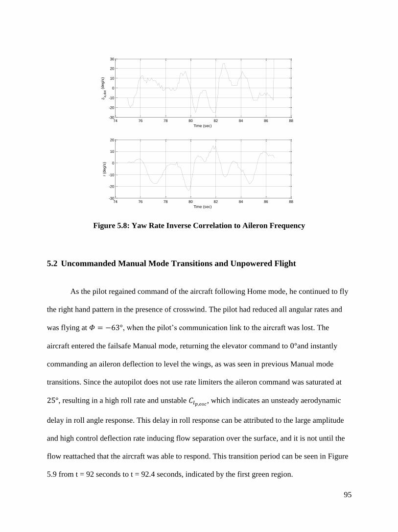
95
Figure 5.8: Yaw Rate Inverse Correlation to Aileron Frequency
5.2 Uncommanded Manual Mode Transitions and Unpowered Flight
As the pilot regained command of the aircraft following Home mode, he continued to fly
the right hand pattern in the presence of crosswind. The pilot had reduced all angular rates and
was flying at , when the pilot’s communication link to the aircraft was lost. The
aircraft entered the failsafe Manual mode, returning the elevator command to and instantly
commanding an aileron deflection to level the wings, as was seen in previous Manual mode
transitions. Since the autopilot does not use rate limiters the aileron command was saturated at
, resulting in a high roll rate and unstable , which indicates an unsteady aerodynamic
delay in roll angle response. This delay in roll response can be attributed to the large amplitude
and high control deflection rate inducing flow separation over the surface, and it is not until the
flow reattached that the aircraft was able to respond. This transition period can be seen in Figure
5.9 from t = 92 seconds to t = 92.4 seconds, indicated by the first green region.
74 76 78 80 82 84 86 88-30
-20
-10
0
10
20
30
Time (sec)
a,d
ot (
deg/s
)
74 76 78 80 82 84 86 88-30
-20
-10
0
10
20
Time (sec)
r (d
eg/s
)
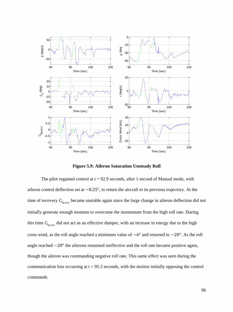
96
Figure 5.9: Aileron Saturation Unsteady Roll
The pilot regained control at t = 92.9 seconds, after 1 second of Manual mode, with
aileron control deflection set at , to return the aircraft to its previous trajectory. At the
time of recovery became unstable again since the large change in aileron deflection did not
initially generate enough moment to overcome the momentum from the high roll rate. During
this time did not act as an effective damper, with an increase in energy due to the high
cross wind, as the roll angle reached a minimum value of and returned to . As the roll
angle reached the ailerons remained ineffective and the roll rate became positive again,
though the aileron was commanding negative roll rate. This same effect was seen during the
communication loss occurring at t = 95.3 seconds, with the motion initially opposing the control
commands.
90 95 100 105
-50
0
50
Time (sec)
p (
deg/s
)
90 95 100 105
-60
-40
-20
0
Time (sec)
(
deg
90 95 100 105
-20
-10
0
10
20
Time (sec)
a (
deg)
90 95 100 105-50
0
50
Time (sec)
r (d
eg/s
)
90 95 100 105
-1
-0.5
0
0.5
1
Time (sec)
Clp
(osc)
90 95 100 105
-20
0
20
40
Time (sec)
Cro
ss W
ind (
kts
)
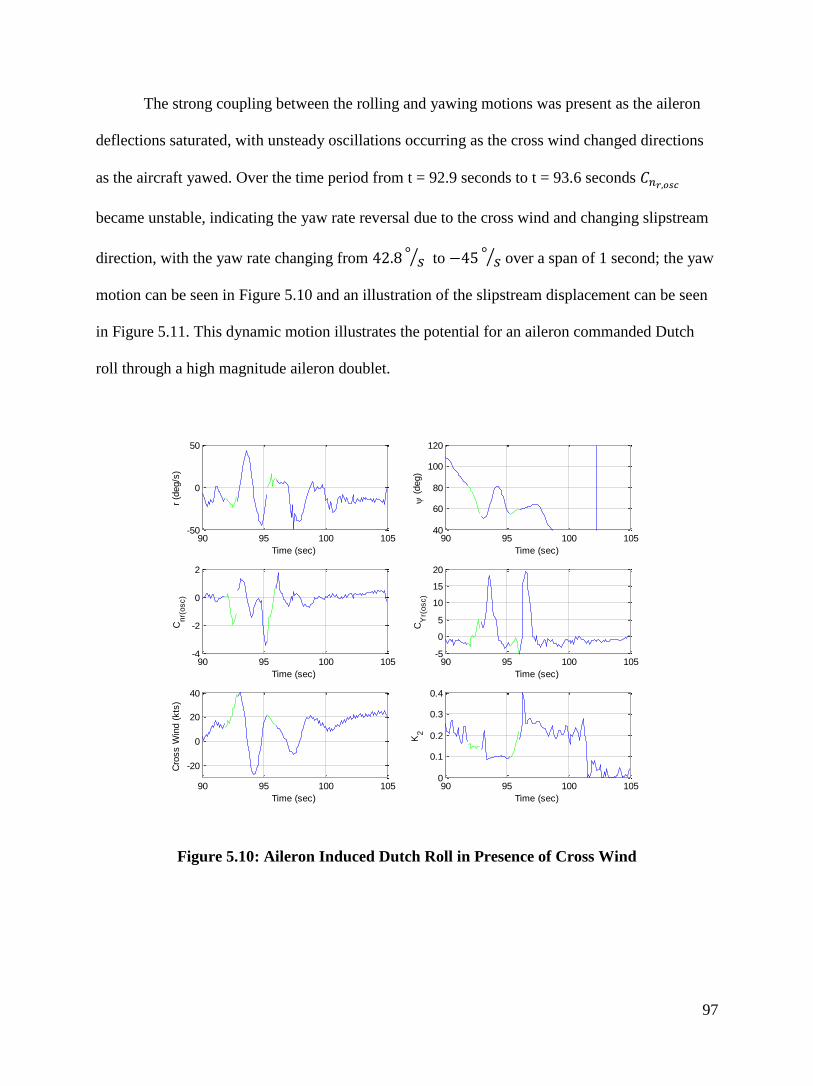
97
The strong coupling between the rolling and yawing motions was present as the aileron
deflections saturated, with unsteady oscillations occurring as the cross wind changed directions
as the aircraft yawed. Over the time period from t = 92.9 seconds to t = 93.6 seconds
became unstable, indicating the yaw rate reversal due to the cross wind and changing slipstream
direction, with the yaw rate changing from ⁄ to
⁄ over a span of 1 second; the yaw
motion can be seen in Figure 5.10 and an illustration of the slipstream displacement can be seen
in Figure 5.11. This dynamic motion illustrates the potential for an aileron commanded Dutch
roll through a high magnitude aileron doublet.
Figure 5.10: Aileron Induced Dutch Roll in Presence of Cross Wind
90 95 100 105-50
0
50
Time (sec)
r (d
eg/s
)
90 95 100 10540
60
80
100
120
Time (sec)
(
deg)
90 95 100 105-4
-2
0
2
Time (sec)
Cnr(
osc)
90 95 100 105-5
0
5
10
15
20
Time (sec)
CY
r(osc)
90 95 100 105
-20
0
20
40
Time (sec)
Cro
ss W
ind (
kts
)
90 95 100 1050
0.1
0.2
0.3
0.4
Time (sec)
K2
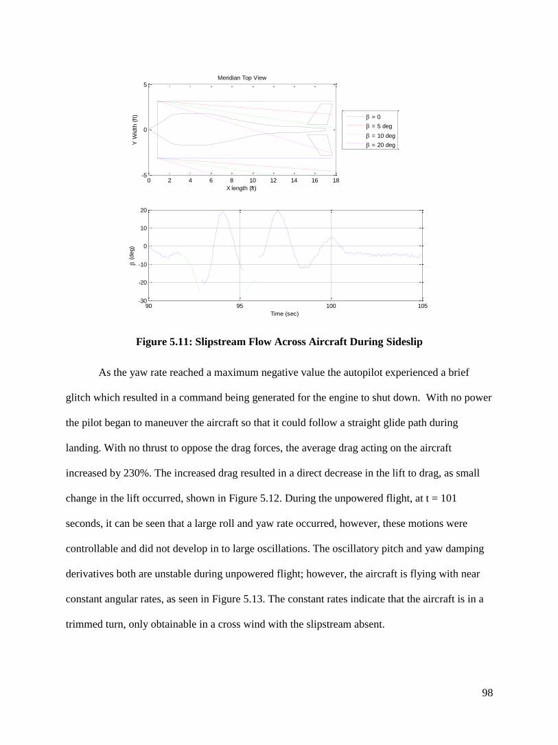
98
Figure 5.11: Slipstream Flow Across Aircraft During Sideslip
As the yaw rate reached a maximum negative value the autopilot experienced a brief
glitch which resulted in a command being generated for the engine to shut down. With no power
the pilot began to maneuver the aircraft so that it could follow a straight glide path during
landing. With no thrust to oppose the drag forces, the average drag acting on the aircraft
increased by 230%. The increased drag resulted in a direct decrease in the lift to drag, as small
change in the lift occurred, shown in Figure 5.12. During the unpowered flight, at t = 101
seconds, it can be seen that a large roll and yaw rate occurred, however, these motions were
controllable and did not develop in to large oscillations. The oscillatory pitch and yaw damping
derivatives both are unstable during unpowered flight; however, the aircraft is flying with near
constant angular rates, as seen in Figure 5.13. The constant rates indicate that the aircraft is in a
trimmed turn, only obtainable in a cross wind with the slipstream absent.
0 2 4 6 8 10 12 14 16 18-5
0
5
X length (ft)
Y W
idth
(ft
)
Meridian Top View
= 0
= 5 deg
= 10 deg
= 20 deg
90 95 100 105-30
-20
-10
0
10
20
Time (sec)
(
deg)
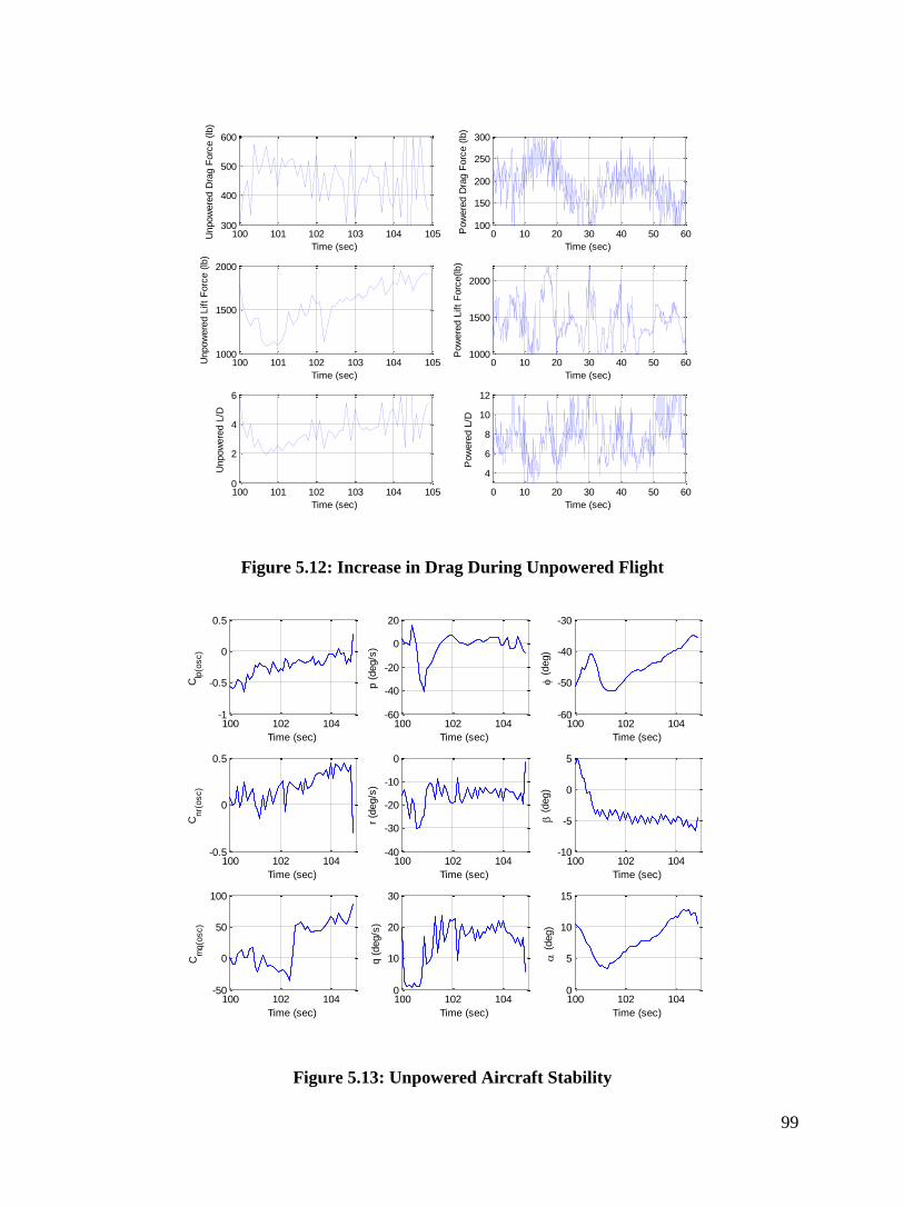
99
Figure 5.12: Increase in Drag During Unpowered Flight
Figure 5.13: Unpowered Aircraft Stability
100 101 102 103 104 105300
400
500
600
Time (sec)
Unpow
ere
d D
rag F
orc
e (
lb)
0 10 20 30 40 50 60100
150
200
250
300
Time (sec)
Pow
ere
d D
rag F
orc
e (
lb)
100 101 102 103 104 1051000
1500
2000
Time (sec)
Unpow
ere
d L
ift
Forc
e (
lb)
0 10 20 30 40 50 601000
1500
2000
Time (sec)
Pow
ere
d L
ift
Forc
e(lb)
100 101 102 103 104 1050
2
4
6
Time (sec)
Unpow
ere
d L
/D
0 10 20 30 40 50 60
4
6
8
10
12
Time (sec)
Pow
ere
d L
/D
100 102 104-1
-0.5
0
0.5
Time (sec)
Clp
(osc)
100 102 104-60
-40
-20
0
20
Time (sec)
p (
deg/s
)
100 102 104-60
-50
-40
-30
Time (sec)
(
deg)
100 102 104-0.5
0
0.5
Time (sec)
Cnr(
osc)
100 102 104-40
-30
-20
-10
0
Time (sec)
r (d
eg/s
)
100 102 104-10
-5
0
5
Time (sec)
(
deg)
100 102 104-50
0
50
100
Time (sec)
Cm
q(o
sc)
100 102 1040
10
20
30
Time (sec)
q (
deg/s
)
100 102 1040
5
10
15
Time (sec)
(
deg)
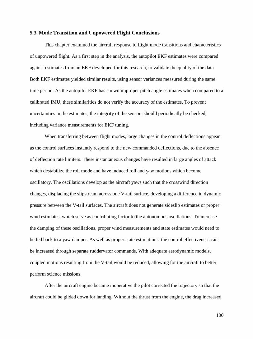
100
5.3 Mode Transition and Unpowered Flight Conclusions
This chapter examined the aircraft response to flight mode transitions and characteristics
of unpowered flight. As a first step in the analysis, the autopilot EKF estimates were compared
against estimates from an EKF developed for this research, to validate the quality of the data.
Both EKF estimates yielded similar results, using sensor variances measured during the same
time period. As the autopilot EKF has shown improper pitch angle estimates when compared to a
calibrated IMU, these similarities do not verify the accuracy of the estimates. To prevent
uncertainties in the estimates, the integrity of the sensors should periodically be checked,
including variance measurements for EKF tuning.
When transferring between flight modes, large changes in the control deflections appear
as the control surfaces instantly respond to the new commanded deflections, due to the absence
of deflection rate limiters. These instantaneous changes have resulted in large angles of attack
which destabilize the roll mode and have induced roll and yaw motions which become
oscillatory. The oscillations develop as the aircraft yaws such that the crosswind direction
changes, displacing the slipstream across one V-tail surface, developing a difference in dynamic
pressure between the V-tail surfaces. The aircraft does not generate sideslip estimates or proper
wind estimates, which serve as contributing factor to the autonomous oscillations. To increase
the damping of these oscillations, proper wind measurements and state estimates would need to
be fed back to a yaw damper. As well as proper state estimations, the control effectiveness can
be increased through separate ruddervator commands. With adequate aerodynamic models,
coupled motions resulting from the V-tail would be reduced, allowing for the aircraft to better
perform science missions.
After the aircraft engine became inoperative the pilot corrected the trajectory so that the
aircraft could be glided down for landing. Without the thrust from the engine, the drag increased

101
by 230%, while the lift remained mostly unchanged. The greatest significance to come from this
unpowered flight is that it validated the idea of the propeller slipstream sustaining the roll and
yaw oscillations. Without the slipstream changing directions with the relative wind, the aircraft
was able to be trimmed, even in the presence of a cross wind.

102
6 Conclusions and Recommendations
Using Fuzzy Logic Modeling, nonlinear and unsteady aerodynamic models have been
generated for the Meridian UAS. The FLM models were used in analyzing flight test for
unsteady, nonlinear, and coupled motion. The following conclusions were made from these data
sets:
High frequency and large magnitude control deflections can cause control induced
oscillations, in both manual and autonomous flight. These oscillations are uncommanded and
often result in high angular rates and the retarding of commanded motions, due to the
unsteady vortices and air relative slipstream interacting at the tail.
The slipstream changing with the relative wind is a large factor in developing unsteady
motion. The propeller diameter is slightly longer than the span of the V-tail , which results in
small cross winds and sideslips causing large dynamic pressure differences between the V-
tail surfaces.
Strong coupling is present between the rolling and yawing motions, which can be induced
through external disturbances or control surface deflections. High yaw rates have shown to
result in an unsteady loss of lift as the motion damps.
AAA is an adequate tool in developing preliminary dynamic aircraft models for large UAS in
steady trimmed flight conditions. The Dutch Roll and short period mode approximations had
error of 20% and 35% for respective natural frequencies, while both damping ratios had
errors of 40%.
Attitude estimations from the Meridian autopilot EKF are inconsistent with estimates from an
auxiliary IMU. Incorrect attitude estimations can negatively affect the generated guidance
and control commands, and makes data analysis challenging.
103
The following recommendations are presented for future research and to aid in future
UAS development:
V-tail configurations should be thoroughly modeled through wind tunnel testing and CFD
analysis, in order to determine the flow interaction between the surfaces at varying
deflections.
V-tails with high dihedral angles should have spans longer than the propeller diameter, as
to reduce the effect of varying slipstream angles in cross winds and sideslips, with the
avoidance of slipstream effects preferable.
V-tail surfaces should be deflected through separate commands to reduce cross-coupled
motion about all three axes, while taking advantage of the coupled control effects.
Rate limiters should be used in the autopilot, to reduce instantaneous large deflections
during mode transitions. This would allow the pilot to gradually regain control of the
aircraft without the control surfaces switching current position on the pilot console.
Control surface feedback should be implemented to determine if the actual surface
deflection is the commanded value. This will aid in determining the presence of flutter or
aerodynamic forces which exceed the capabilities of the servos.
Sensor integrity should periodically be assessed, including adjustments to the EKF.
Furthermore autopilot commands generated with respect to the relative wind,
necessitating the use of air flow angle sensors in the free stream and at the V-tail.
Further research should be performed to assess the longitudinal motions of the Meridian
UAS, as this work has primarily focused on lateral-directional motion.
104
Works Cited
[1] "About CReSIS," 2013. [Online]. Available: https://www.cresis.ku.edu/about. [Accessed 20
November 2013].
[2] K. Byers, J. A. R. Harish, S. A. Seguin, C. Leuschen, F. Rodriguez-Morales, J. Paden, E.
Arnold and R. Hale, "A Modified Wideband Dipole Antnna for an Airborne VHF Ice
Penetrating Radar," IEEE Transactions on Instrumentation and Measurement, vol. 61, no.
5, pp. 1435-1444, 2012.
[3] B. Panzer, D. Gomez-Garcia, C. Leushcen, J. Paden, F. Rodriguez-Morales, A. Patel, T.
Markus, B. Holt and P. Gogineni, "An Ultra-Wideband, Microwave Radar for Measuring
Snow Thickness on Sea Ice and Mapping Near-Surface Internal Laers in Polar Firn,"
Journal of Glaciology, vol. 59, no. 214, pp. 244-254, 2013.
[4] F. Rodriguez-Morales, S. Gogineni, C. Leuschen, J. Paden, J. Li, C. Lewis, B. Panzer, D.
Gomez-Garcia, A. Patel and K. Byers, "An Advanced Multi-Frequency Radar
Instrumentation for Polar Research," IEEE Transactions on Geoscience and Remote
Sensing, vol. PP, no. 99, pp. 1-19, 2013.
[5] F. M. Nick, A. Vieli, M. L. Anderson, I. Joughin, A. Payne, T. L. Edwards, F. Pattyn and R.
S. W. van de Wal, "Future Sea-Level Rise From Greenland's Main Outlet Glaciers in a
Warming Climate," Nature, vol. 497, no. 7448, pp. 235-238, 2013.
[6] R. T. Walker, D. M. Holland, B. R. Parizek, R. B. Alley, S. M. J. Nowicki and A. Jenkins,
"Efficient Flowline Simulations of Ice Shelf-Ocean Interactions: Sensitivity Studies with a
Fully Coupled Model," Journal of Physical Oceanography, vol. 43, no. 10, pp. 2200-2210,
2013.
[7] M. McDaniel, E. Sprout, D. Boudreau and A. Turgeon, "Climate Refugee," National

105
Geographic Education Programs, [Online]. Available:
http://education.nationalgeographic.com/education/encyclopedia/climate-refugee/?ar_a=1.
[Accessed January 2013].
[8] "Wind in Antarctica," British Antarctic Survey, [Online]. Available:
http://www.antarctica.ac.uk/about_antarctica/geography/weather/wind.php. [Accessed 13
January 2014].
[9] Steffen Research Group, "Greenland Climate Network," Cooperative Institute for Research
in Environmental Sciences, Boulder, 2014.
[10] C. E. Lan, S. Keshmiri and R. Hale, "Fuzzy-Logic Modeling of a Rolling Unmanned
Vehicle in Antarctica Wind Shear," AIAA Journal of Guidance, Control, and Dynamics, vol.
35, no. 5, pp. 1538-1547, 2012.
[11] "Antarctica Crash Plane Too Dangerous to Recover, say Officials," The Canadian Press, 27
January 2013.
[12] W. R. Donovan and R. D. Hale, "Meridian: An Unihabited Air Vehicle for Use in Polar
Research," in 48th AIAA/ASME/ASCE/AHS/ASC Strucures, Structural Dynamics and
Materials Conference, Honolulu, 2007.
[13] R. D. Hale, W. R. Donovan, M. Ewing, K. Siegele, R. Jager, E. Leong and W. B. Liu, "The
Meridian UAS: Detailed Design Review," CReSIS Technical Report, no. 124, p. 79,
06/2007.
[14] W. Donovan, "CReSIS UAV Critical Design Review: The Meridian," CReSIS Technical
Report, no. 123, p. 88, 06/2007.
[15] W. Donovan, "CReSIS UAV Preliminary Design Review: The Meridian," CReSIS
Technical Report, no. 125, p. 137, 06/2007.
106
[16] G. A. Garcia, S. Keshmiri and R. D. Colgren, "H-Infinity Gain Scheduling Design for the
Meridian UAS for a Broader Range of Operation and for Fault Tolerant Applications," in
9th IEEE International Conference on Control and Automation, Santiago, 2011.
[17] R. F. Stengel, Flight Dynamics, Princeton: Princeton University Press, 2004.
[18] J. Roskam, Airplane Flight Dynamics and Automatic Flight Controls Part I, 5th ed.,
Lawrence: Design, Analysis, and Research Corporation, 2007.
[19] D. Sheu and C.-T. Lan, "Estimation of Turbulent Vertical Velocity from Nonlinear
Simulations of Aircraft Response," AIAA Journal of Aircraft, vol. 48, no. 2, pp. 645-651,
2011.
[20] J. Li and C. E. Lan, "Unsteady Aerodynamic Modeling of Aircraft Response to
Atmospheric Turbulence," in AIAA Atmospheric Flight Mechanics Conference and Exhibit,
Austin, 2003.
[21] C. E. Lan, "aeroid35.exe".
[22] T. Theodorsen, "General Theory of Aerodynamic Instability and the Mechanism of Flutter,"
NACA TR 496, 1934.
[23] Z. Wang and C. E. Lan, "Fuzzy Logic Modeling of Nonlinear Unsteady Aerodynamics,"
AIAA-98-4351, 1998.
[24] Z. Wang and C. E. Lan, "Unsteady Aerodynamic Effects on the Flight Characteristics of an
F-16XL Configuration," AIAA-2000-3910, 2000.
[25] C. E. Lan, "rfreq34.exe".
[26] B. G. Van Der Wall and J. Leishman, "On the Influence of Time-Varying Flow Velocity on
Unsteady Aerodynamics," Journal of the American Helicopter Society, vol. 39, no. 4, pp.
25-36, 1994.
107
[27] R. Jategaonkar, Flight Vehicle System Identification, AIAA, 2006.
[28] V. Klein, Aircraft System Identification Theory and Practice, AIAA, 2006.
[29] M. Tischler and R. Remple, Aircraft and Rotorcraft System Identifcation, AIAA, 2012.
[30] C. E. Lan, "modelg34.exe".
[31] J. Kalviste, "Use of Rotary Balance and Forced Oscillation Test Data in a Six Degrees of
Freedom Simulation," in AIAA 9th Atmospheric Flight Mechanics Conference, San Diego,
1982.
[32] O. Zikanov, Essential Computational Fluid Dynamics, John Wiley & Sons, 2011.
[33] Langley Research Center, "Vortex-Lattic Utilization," in A Workshop Held at Langley
Research Center, Hampton, 1976.
[34] M. Drela and H. Youngren, Athena Vortex Lattice (Software), Cambridge: MIT, 1988-2004.
[35] DAR Corporation, "Advanced Aircraft Analysis," [Software].
[36] "Advanced Aircraft Analysis," DAR Corporation, [Online]. Available:
http://www.darcorp.com/Software/AAA/. [Accessed 9 September 2013].
[37] R. Lykins, R. Riley, G. Garcia and S. Keshmiri, "Modal Analysis of 1/3-Scale Yak-54
Aircraft Through Simulation and Flight Testing," in AIAA Atmospheric Flight Mechanics
Conference, Portland, 2011.
[38] J. John D. Anderson, Fundamentals of Aerodynamics, 4th ed., New York: McGraw-Hill,
2007.
[39] W. F. Phillips, Mechanics of Flight, Hoboken: John Wiley & Sons, Inc., 2004.
[40] V. J. Rossow, "Classical Wing Theory and the Downward Velocity of Vortex Wakes,"
AIAA Journal of Aircraft, vol. 43, no. 2, pp. 381-385, 2006.
108
[41] M. R. Visbal, "Analysis of the Onset of Dynamic Stall Using High-Fidelity Large-Eddy
Simulations," in AIAA 52nd Aerospace Sciences Meeting, National Harbor, 2014.
[42] M. R. Visbal, "Three-Dimensional Flow Structure on a Heaving Low-Aspect-Ratio Wing,"
in 49th AIAA Aerospace Sciences Meeting, Orlando, 2011.
[43] M. R. Visbal, "High-Fidelity Simulation of Transitional Flows Past a Plunging Airfoil," in
47th AIAA Aerospace Sciences Meeting, Orlando, 2009.
[44] M. R. Visbal, "Flow Structure and Unsteady Loading Over a Pitching and Perching Low-
Aspect-Ratio Wing," in 42nd AIAA Fluid Dynamics Conerence and Exhibit, New Orleans,
2012.
[45] C. Liang, K. Ou, P. Sachin, J. Antony and Z. J. Wang, "High-Order Accurate Simulations of
Unsteady Flow Past Plunging and Pitching Airfoils," Computers and Fluids, vol. 40, pp.
236-248, 2011.
[46] Department of Defense Interface Standard, Flying Qualities of Piloted Aircraft, MIL-STD-
1797A Notice 3, 2004.
[47] D. A. Johnson, "Suppression of Pilot-Induced Oscillation (PIO)," Air Force Institute of
Technology, Wright-Patterson Air Force Base, 2002.
[48] D. G. Mitchell and D. H. Klyde, "Identifying a Pilot-Induced Oscillation Signature: New
Techniques Applied to Old Problems," AIAA Journal of Guidance, Control, and Dynamics,
vol. 31, no. 1, pp. 215-224, 2008.
[49] T. Mandal, Y. Gu, H. Chao and M. Rhudy, "Flight Data Analysis of Pilot-Induced-
Oscillations of a Remotely Controlled Aircraft," in AIAA Guidance, Navigation, and
Control Conference, Boston, 2013.
[50] K. W. Williams, "A Summary of Unmanned Aircraft/Incident Data; Human Factors
109
Implications," U.S. Department of Transportation/Federal Aviation Administration,
Washington, D.C., 2004.
[51] D. G. Mitchell, "Identifying the Pilot in Pilot-Induced Oscillations," in AIAA Atmospheric
Flight Mechanics Conference, Denver, AIAA-2000-3985.
[52] D. G. Mitchell, A. J. Arencibia and S. Munoz, "Real-Time Detection of Pilot-Induced
Oscillations," in AIAA Atmospheric Flight Mechanics Conference and Exhibit, Providence,
2004.
[53] E. Kreyszig, Advanced Engineering Mathematics, 10th ed., Hoboken: John Wiley & Sons,
Inc., 2011.
[54] W. F. Phillips, A. B. Hansen and W. M. Nelson, "Effects of Tail Dihedral on Static
Stability," Journal of Aircraft, vol. 43, no. 6, pp. 1829-1837, 2006.
[55] B. C. Sweeten, "CFD Analysis of UAVs using VORSTAB, FLUENT, and Advanced
Aircraft Analysis," KU ScholarWorks, Lawrence, 2010.
[56] M. Rhudy, Y. Gu and M. Napolitano, "Relaxation of Stability Requirements for Extended
Kalman Filter Stability within GPS/INS Attitude Estimation," in AIAA Guidance,
Navigation, and Control Conference, National Harbor, 2014.
[57] R. E. Gordnier and M. R. Visbal, "Numerical Simulation of the Impingement of a
Streamwise Vortex on a Plate," AIAA-97-1781, 1997.
[58] B. R. Kramer, "Experimental Evaluation of Superposition Techniques Applied to Dynamic
Aerodynamics," in 40th AIAA Aerospace Sciences Meeting & Exhibit, Reno, 2002.
[59] Y.-N. Lee and C. E. Lan, "Analysis of Random Gust Response with Nonlinear Unsteady
Aerodynamics," AIAA Journal, vol. 38, no. 8, pp. 1305-1312, August 2000.
[60] J. Roskam, Airplane Design Part VI: Preliminary Calculations of Aerodynamic, Thrust and
110
Power Characteristics, 5th ed., Lawrence: Design Analysis and Research Corporation, 2008.
[61] S. Chin and C. E. Lan, "Fourier Functional Analysis for Unsteady Aerodynamic Modeling,"
AIAA Journal, vol. 30, no. 9, pp. 2259-2266, 1992.
[62] C. E. Lan, "Dynamic Aerodynamics," Journal of Aeronautics, Astronautics and Aviation,
Series A, vol. 38, no. 4, pp. 217-24, 2006.
[63] A. M. Murch and J. V. Foster, "Recent NASA Research on Aerodynamic Modeling of Post-
Stall and Spin Dynamics of Large Tansport Airplanes," in 45th AIAA Aerospace Sciences
Meeting and Exhibit, Reno, 2007.
[64] C.-H. Hsu and C. E. Lan, "Theory of Wing Rock," AIAA Journal of Aircraft, vol. 22, no. 10,
pp. 920-924, 195.
[65] R. C. Chang, C.-E. Ye, C. E. Lan and M. Guan, "Flying Qualities for a Twin-Jet Transport
in Severe Atmospheric Turbulence," AIAA Journal of Aircraft, vol. 46, no. 5, pp. 1673-
1680, 2009.
[66] C. E. Lan, "modelg34.exe".
[67] C. E. Lan, "prederv35.exe".
[68] C. E. Lan, "strucg34.exe".
[69] R. Y. Myose and J. Iwata, "The Near-Wake Flow Behavior of an Oscillating Airfoil with
Modified Trailing Edge," in 33rd Aerospace Sciences Meeting and Exhibit, Reno, AIAA
95-0308.