Odour and Ammonia Emission from Broiler Farms A report for the Rural Industries Research and Development Corporation by John K Jiang and John R Sands February 2000 RIRDC Publication No 00/2 RIRDC Project No UNS-11A

ii

© 2000 Rural Industries Research and Development Corporation. All rights reserved. ISBN 0 642 580 324 ISSN 1440-6845 Odour and Ammonia Emission from Broiler Farms Publication No. 00/2 Project No. UNS-11A The views expressed and the conclusions reached in this publication are those of the author and not necessarily those of persons consulted. RIRDC shall not be responsible in any way whatsoever to any person who relies in whole or in part on the contents of this report. This publication is copyright. However, RIRDC encourages wide dissemination of its research, providing the Corporation is clearly acknowledged. For any other enquiries concerning reproduction, contact the Publications Manager on phone 02 6272 3186. Researcher Contact Details John Jiang Centre for Water and Waste Technology The School of Civil and Environment Engineering The University of NSW Sydney 2052 Phone: (02) 9385 5452 Fax: (02) 9313 8624 Email: j.jiang@unsw.edu.au Website: http://www.odour.civeng.unsw.edu.au

RIRDC Contact Details Rural Industries Research and Development Corporation Level 1, AMA House 42 Macquarie Street BARTON ACT 2600 PO Box 4776 KINGSTON ACT 2604 Phone: 02 6272 4539 Fax: 02 6272 5877 Email: rirdc@rirdc.gov.au. Website: http://www.rirdc.gov.au Published in February 2000 Printed on environmentally friendly paper by Canprint

iii

Foreword

The Chicken Meat Committee of RIRDC in 1996 commissioned the Environmental Odour Laboratory at the Centre for Waste Water Treatment, School of Civil and Environment Engineering, The University of New South Wales, to undertake a project for which the initial objectives were to quantify, in an objective way, odour and ammonia emission in and adjacent to some typical chicken meat farms and to identify and make recommendations on potential remedial measures with a particular focus on operational and management aspects.

The Environmental Odour Laboratory has some of the best available technology for odour measurement and uses the Dutch Standard NVN 2820 for its olfactory measurements. While undertaking the study, the Environmental Odour Laboratory was accredited by the National Association of Testing Authorities, Australia for the Dutch Standard NVN 2820 method of olfactometry (results reported as per draft Aust Standard, as “Certain and Correct” criteria). The Dutch Standard is the basis for the development of the proposed European Standard and the proposed Australian Standard for odour measurement. Consequently the data presented in this report should be useable for some time to come, rather than becoming dated by the use of an Australian state based method or other method with limited international acceptance.

The primary outcomes of the project have been the development of a database of information on odour emission rates, odour intensities and ammonia emissions associated with broiler farms and the development of an improved understanding of odour generation and dispersion from broiler farms.

The research undertaken did not seek to elucidate the fundamental mechanisms of odour generation in broiler farms, to determine how odours can be minimised at their source or how odour dispersion can be enhanced by design of chicken production facilities. These aspects may be the subjects of future research and development projects supported by RIRDC. Furthermore, while odour concentrations were measured in a number of different shed ventilation configurations, there are an inadequate number of data sets to provide meaningful comparisons between shed types.

As part of the work undertaken and reported upon in this document, some preliminary odour dispersion modelling was undertaken on the odour emission data collected to facilitate an understanding of odour impacts associated with broiler farms.

This report, a new addition to RIRDC’s diverse range of over 450 research publications, forms part of our (fill in relevant program) R&D program, which aims to (fill in program’s objective).

Most of our publications are available for viewing, downloading or purchasing online through our website:

• downloads at www.rirdc.gov.au/reports/Index.htm • purchases at www.rirdc.gov.au/pub/cat/contents.html

Peter Core Managing Director Rural Industries Research and Development Corporation

iv

Acknowledgments External funding for the project was provided by the Rural Industries Research and Development Corporation through its Chicken Meat Program. The University of New South Wales provided support by way of laboratory facilities, office services and library and information services. The authors gratefully acknowledge the generous support of these two bodies.

The authors would like to record their sincere thanks to the members and other participants in the many meetings of the project steering committee and to members of the chicken meat industry generally for their valuable contributions to the project. Their rich industry experience has proved invaluable in determining the direction of the project and developing a practical experimental design.

Special thanks are due to the six New South Wales and five Victorian growers, together with the Tocal Agricultural College, for providing farms for study purposes and for suffering the inevitable disruption to farming operations from the research procedures.

The contribution of local residents in the conduct of the odour community survey is also gratefully acknowledged.

Particular thanks are due to Steggles for providing a weather station for use on one of the farms studied together with meteorological data from their Beresfield processing plant and to Inghams for allowing us to undertake a study in conjunction with their feed trials. Several state agricultural and environmental agencies provided significant input and, in particular, the Victorian Environment Protection Authority provided assistance in relation to field data collection and modelling.

A major contribution to the work program of the project team was provided by Tamir J M Xiao who undertook field work and olfactometry testing for the project. Another team member, Colin Parker, located in the Hunter Valley provided outstanding input, particularly in respect to the community survey but also in undertaking tasks requiring local knowledge of chicken growing operations.

v

Glossary

Air Exchange Rate (AER): Number of times per hour, total volume of air inside shed is exchanged with air outside shed.

Ausplume: An air dispersion model developed by the Victorian Environment Protection Authority. (The current version, Version 4.0.)

Break point: See Individual threshold.

Centre for Water and Wastewater Treatment (CWWT): Centre for Water and Wastewater Treatment at the University of New South Wales.

Cross ventilated shed: Shed provided with mechanical ventilation across its medial axis. Detection threshold: Odorant concentration that has a probability of 0.5 of being detected.

Dilution ratio: Ratio between flow or volume after dilution and the flow or volume of an odorous gas.

Dynamic olfactometry: Olfactometry using a dynamic olfactometer.

Individual threshold: Detection threshold applying to an individual.

Integrator or integrator company: Vertically integrated company that owns chickens and provides food and other inputs to the farmer to growout newly hatched chickens until picked up by integrator for killing and processing.

Mechanically ventilated shed: Shed provided with mechanical ventilation. Naturally ventilated shed: Shed using natural forces produced by operation of shed openings together with energy from ambient wind, temperature and direct radiant energy, to achieve ventilation.

Odour annoyance: Odour impact perceived by a receptor as unpleasant.

Odour concentration: Number of odour units per unit of volume. The numerical value of the odour concentration is equal to the number of dilutions to arrive at the odour threshold. (ou/m3)

Odour detection threshold (Co): An estimate of the odour detection threshold concentration.

Odour emission rate: Product of shed odour concentration measured by olfactometer and the shed ventilation (ou/sec).

Odour impact limits: A general term including odour design goal, odour annoyance criteria, and odour performance criteria.

Odour impact criteria: Parameters including odour concentration, exceedance probability, averaging time and receptor location used to provide objective means for defining odour impact area in which perceived odour likely exceeds distinct level for a limited time in a year.

Odour impact: Effect perceived by an individual receptor or group of receptors at a distance from an odour emission source.

Odour intensity: The intensity of sensation stimulated by an odorant as assessed on a scale of 0 1 2 3 4 5 6.

Odour nuisance threshold: Odour concentration at which perceived odour intensity reaches a value of 3, the level at which an odour is perceived by a panellist to be distinct.

Odour strength: The strength of an environmental odour determined as an odour concentration (ie the number of times a sample of air carrying the environmental odour needs to be diluted to arrive at the odour threshold). By definition the odour threshold corresponds to an odour concentration of one odour unit per cubic metre (ie 1 ou/m3).

Odour unit: Quantity of a gaseous substance or mixture of substances which, when evaporated into 1 m3, is distinguished from odourless air by half the panel members.

Olfactometer: Apparatus in which a sample of odorous gas is diluted with neutral gas in a defined ratio and presented to an odour panel.

Separation distance: Minimum distance between a group of sheds and a specified potential odour receptor.

Stevens law: A law defining the perceived psychological intensity as a function of odorant concentration.

Tunnel ventilated shed: Shed provided with mechanical ventilation along its longitudinal axis to achieve improved air exchange and enhanced wind chill. Ventilation rate: Ventilation rate for a shed is the product of the measured exhaust air velocity and the cross sectional area of the opening or openings through which exhaust air leaves the shed.

vi

Contents FOREWORD .......................................................................................................................................III

ACKNOWLEDGMENTS......................................................................................................................... IV

GLOSSARY ....................................................................................................................................... V

EXECUTIVE SUMMARY........................................................................................................................ XI

1. INTRODUCTION ..................................................................................................................................1

2. OBJECTIVES .......................................................................................................................................2

3. ODOUR FROM BROILER FARMS......................................................................................................3

3.1 The nature of odours ........................................................................................................................3

3.2 Broiler growth cycle ..........................................................................................................................4

3.3 Broiler farm odour generation...........................................................................................................4

3.4 Ventilation.........................................................................................................................................6

3.5 Management practice.......................................................................................................................7

3.6 Typical buffer distances adopted for broiler farms in Australia ........................................................7

4. METHODOLOGY .................................................................................................................................9

4.1 Project design...................................................................................................................................9 4.1.1. Full year emission study at two farms .....................................................................................10 4.1.2. Twelve farm spot emission survey ..........................................................................................10 4.1.3. Odour community survey ........................................................................................................10 4.1.4. Feed study...............................................................................................................................11

4.2 Temperature, humidity, moisture and air velocity measurement ...................................................12

4.3 Ventilation rate calculation .............................................................................................................14

4.4 Ammonia concentration measurement...........................................................................................14

4.5 Sampling from litter surface............................................................................................................15

4.6 GC-MS analysis..............................................................................................................................16

4.7 Litter moisture content....................................................................................................................17

4.8 Meteorological station ....................................................................................................................17

4.9 Odour concentration measurement................................................................................................18 4.9.1 Sample collection and transport...............................................................................................19 4.9.2 Olfactometry testing .................................................................................................................20 4.9.3 Odour-free test environment ....................................................................................................20 4.9.4 Panellist management..............................................................................................................21 4.9.5 Olfactometer calibration ...........................................................................................................21 4.9.6 Olfactometer results calculation ...............................................................................................21 4.9.7 Odour emission rate calculation...............................................................................................23

4.10 Odour intensity measurement ......................................................................................................23

4.11 Odour dispersion modelling..........................................................................................................25 4.11.1 Odour emission rates .............................................................................................................27 4.11.2 Averaging time .......................................................................................................................27 4.11.3 Source characteristics ............................................................................................................27 4.11.4 Receptor locations..................................................................................................................29 4.11.5 Meteorological data ................................................................................................................29 4.11.6 Limitations of Ausplume for modelling odour generated by broiler farms..............................29

4.12 Development of odour impact criteria...........................................................................................29

4.13 Community survey........................................................................................................................31

vii

5. DETAILED RESULTS ........................................................................................................................32

5.1 Temperature and Humidity.............................................................................................................32

5.2 Ammonia concentration at different positions inside a shed..........................................................33

5.3 Ammonia concentration in a single batch ......................................................................................33

5.4 Ammonia concentration from litter surface.....................................................................................35

5.5 Litter moisture.................................................................................................................................36

5.6 Feed trial.........................................................................................................................................37

5.7 GC-MS results ................................................................................................................................37

5.8 Farm survey results ........................................................................................................................37

5.9 Odour concentration inside sheds in relation to season ................................................................39

5.10 Ventilation rate for naturally ventilated shed ................................................................................40

5.11 Ventilation rate for tunnel ventilated shed ....................................................................................42

5.12 Odour dispersion modelling results ..............................................................................................44

5.13 Sensitivity of odour dispersion modelling results to some alternative odour emission rate assumptions...........................................................................................................49

5.14 Odour intensity results..................................................................................................................52

5.15 Odour community survey .............................................................................................................54

6. DISCUSSION OF RESULTS .............................................................................................................55

6.1 Temperature and humidity within broiler shed ...............................................................................55

6.3 Odour concentration levels inside sheds on various farms............................................................58

6.4 GC-MS analysis..............................................................................................................................59

6.5 Feed trial.........................................................................................................................................59

6.6 Ventilation rates..............................................................................................................................60

6.7 Odour dispersion modelling............................................................................................................61

6.8 Odour intensity ...............................................................................................................................62

6.9 Community survey..........................................................................................................................62

6.10 Odour impact radius .....................................................................................................................63

7. IMPLICATIONS ..................................................................................................................................65

8. RECOMMENDATIONS ......................................................................................................................66

9. REFERENCES AND BIBLIOGRAPHY ..............................................................................................67

APPENDICES ......................................................................................................................................71

Appendix 1: Data from NSW study.......................................................................................................71

Appendix 2: NSW Farm conditions ......................................................................................................72

Appendix 3: Data from Victoria study...................................................................................................73

Appendix 4: Victoria Farm conditions...................................................................................................74

Appendix 5: GC-MS Results ................................................................................................................83

Appendix 6: Odour community survey letter and forms .......................................................................86

Appendix 7: Odour concentration during the transportation.................................................................90

Appendix 8: Photographs .....................................................................................................................92

viii

List of Figures Figure 1 Typical air temperature profile over a broiler growout batch......................................................5

Figure 2 Arrangement for data logging..................................................................................................12

Figure 3 Typical placements of sensors................................................................................................13

Figure 4 Arrangement for ammonia sampling.......................................................................................15

Figure 5 Isometric drawing of portable wind tunnel system .................................................................15

Figure 6 Calibration of Theta Probe against gravimetric method..........................................................17

Figure 7 Odour sampling system ..........................................................................................................20

Figure 8 Simulated panellist screening results......................................................................................21

Figure 9 Odour intensity versus odour concentration ...........................................................................23

Figure 10 Illustration of odour plume from a tunnel ventilated shed .....................................................28

Figure 11 Temperature and humidity inside shed at Farm NB over 17 days........................................32

Figure 12 Ammonia concentration at different locations along a shed on nine days............................33

Figure 13 Ammonia concentration in shed for several batches at Farms NA and NB..........................34

Figure 14 Ammonia concentration and bird weight at Farm NB ...........................................................34

Figure 15 Ammonia concentration and bird weight at Farm NA ...........................................................35

Figure 16 Ammonia concentration at litter surface for batches at Farm NA .........................................35

Figure 17 Odour concentration and litter moisture at NSW farms ........................................................36

Figure 18 Odour concentration and litter moisture at Victorian farms...................................................36

Figure 19 Odour concentration in sheds at eight farms in NSW...........................................................38

Figure 20 Odour concentration in shed at five farms in Victoria ...........................................................39

Figure 21 Odour concentration related to season at two NSW farms...................................................39

Figure 22 Typical air velocity over two days at Farm NA at side openings...........................................40

Figure 23 Air velocity at Farm NB over 17 days....................................................................................40

Figure 24 Hourly average at Farm NB over 17 days.............................................................................41

Figure 25 Air velocity at Farm NA .........................................................................................................41

Figure 26 Air velocity at Farm VC .........................................................................................................42

Figure 27 Correlation between measured air velocity at shed cross-section area against number of fans in operation ...............................................................................................................43

Figure 28 Hourly odour concentration isopleths at the 99.5th percentile for Farm NA in NSW............45

Figure 29 Hourly odour concentration isopleths at the 99.5th percentile for Farm NB in NSW............46

Figure 30 Hourly odour concentration isopleths at the 99.5th percentile for Farm VA in Victoria ........46

Figure 31 Hourly odour concentration isopleths at the 99.5th percentile for Farm VB in Victoria ........47

Figure 32 Hourly odour concentration isopleths at the 99.5th percentile for Farm VC in Victoria ........47

ix

Figure 33 Hourly odour concentration isopleths at the 99.5th percentile for Farm VD in Victoria ........48

Figure 34 Hourly odour concentration isopleths at the 99.5th percentile for Farm VE in Victoria ........48

Figure 35 Odour impact isopleths for alternative scenario NVAb .........................................................50

Figure 36 Odour impact isopleths for alternative scenario NVAc..........................................................50

Figure 37 Odour impact isopleths for alternative scenario NVAd .........................................................51

Figure 38 Odour impact isopleths for alternative scenario NVAe .........................................................51

Figure 39 Grouping of residences in odour community survey around Farm NA.................................54

Figure 40 Odour annoyance index by residence number .....................................................................54

Figure 41 Air velocities and ammonia concentration in WA farm (First night) ......................................56

Figure 42 Air velocities and ammonia concentration in WA farm (Second night) .................................56

Figure 43 Sample temperature recorded during the transportation from Darwin to Sydney on 5 July 1999 ..............................................................................................................................59

Figure 44 Correlation between odour impact radius and nominal farm broiler capacity for an odour concentration of 5 ou/m3 at the 99.5th percentile......................................................64

Figure 45 GC-MS Chromatogram for sample 3 and 4..........................................................................83

Figure 46 GC-MS Chromatogram for sample 5....................................................................................84

Figure 47 GC-MS Chromatogram for sample 6....................................................................................84

Figure 48 GC-MS Chromatogram for sample 7....................................................................................85

Figure 49 GC-MS Chromatogram for sample 8....................................................................................85

x

List of Tables Table 1 Typical guidelines or requirements for separation distances for broiler farms...........................8

Table 2 Annoyance categories and weighting factors...........................................................................11

Table 3 Protein content of feed mixes used in feed trials. ....................................................................11

Table 4 Details of temperature, humidity, and air velocity sensors.......................................................13

Table 5 Weather station configurations..................................................................................................18

Table 6 Odour concentration calculation demonstration.......................................................................22

Table 7 Odour intensity criteria .............................................................................................................24

Table 8 Illustration of odour intensity measurement calculation (one sample) .....................................25

Table 9 Odour emission rates as a function of ambient temperature ...................................................27

Table 10 Some odour impact criteria used in several jurisdictions .......................................................29

Table 11 Convention adopted linking batch stage in weeks to bird age in days...................................32

Table 12 Schedule of ammonia sampling ............................................................................................33

Table 13 Kjedahl Nitrogen results .........................................................................................................37

Table 14 Ammonia concentration at litter surface.................................................................................37

Table 15 Major compounds determined by GC-MS analysis................................................................38

Table 16 Summary of ventilation rates from naturally ventilated sheds................................................42

Table 17 Summary of ventilation rates from mechanically ventilated shed ..........................................43

Table 18 Summary of meteorological data at the studied farms...........................................................44

Table 19 Estimated worst case (Week 6) odour emission rates used in modelling..............................44

Table 20 Summary of farm conditions...................................................................................................45

Table 21 Alternative scenarios modelled for naturally ventilated sheds ...............................................49

Table 22 Odour intensity at NSW farms................................................................................................53

Table 23 Odour intensity at Victorian farms ..........................................................................................52

Table 24 Summary of odour impact radii for NSW and Victorian farms ...............................................63

Table 25 Alternative scenarios demonstrating effect of varying odour emission rate assumptions in modelling...........................................................................................................................63

xi

Executive Summary

During the period of January 1997 to June 1998, two New South Wales broiler farms were studied over four seasons and a further ten broiler farms in New South Wales and Victoria were surveyed at week 6 of a batch. The project studied spatial and temporal variations in ammonia concentration within the broiler sheds and developed an odour sampling procedure for the broiler farms. Improved odour impact assessment procedures were developed for predicting odour impact from broiler farms. A database of broiler farm odour emissions was established and the odour impact from broiler farms was predicted using scientifically derived odour impact criteria. Since the odour testing procedure complies with the proposed Australian standard for odour measurement, the database can be used by the broiler industry for many years to come.

For naturally ventilated sheds, the spatial, diurnal and weekly variations of ammonia were during a typical eight weeks growout batch. Ammonia was analysed on site by wet chemistry immediately after the samples were collected. Taking into account data obtained in a parallel study of Western Australian broiler farms undertaken by the authors, three major findings were observed:

• Ammonia concentration was observed to be reasonably evenly distributed within a shed at all stages of a batch of chickens.

• Ammonia concentration was found to vary greatly on a diurnal pattern with the opening and closing of sheds on any particular day.

• Ammonia concentration levels within a shed were recorded to reach a plateau at the time (typically at Week 6) that the total bird biomass reached a maximum on a batch basis.

• Results obtained indicated that a composite odour sample could be taken as representative of the average odour concentration within the shed at one time. It is also concluded that three composite odour samples (taken early morning, early afternoon and early evening) on a day in Week 6 could be used to represent maximum odour concentration levels for a growout batch.

A total of 88 odour concentration samples and 29 odour intensity samples were analysed by dynamic olfactometry using the Dutch standard NVN 2820 (based on certainty and correct criteria) and German VDI 3882 respectively. The ventilation rate, air humidity, temperature and litter moisture in sheds were also measured. The results show that odour concentrations were in the range of 50 – 1000 ou/m3, and varying with ventilation rates, litter moisture level, and shed design.

Gas compositions inside the broiler sheds were analysed by GC-MS. Results confirmed that ammonia and dimethyl disulfide were, by volume, the major odorous constituents inside the broiler sheds.

An odour impact assessment procedure was developed using laboratory measurement and a community survey. To take into account diurnal variation in odour emissions from broiler sheds for modelling purposes, odour emission rates from a single shed were assumed to be at a maximum value when ambient temperatures were above 15 °C, dropping to 10% of the maximum rate at ambient temperatures of 15 °C and lower. The maximum odour emission rate was calculated from the maximum ventilation rate and averaged odour concentrations measured inside the shed. Odour emission rates from a farm were estimated from the air exchange rate corresponding to the maximum ventilation rate and averaged odour concentrations. The odour concentration component of the odour impact criteria was derived from the perceived odour intensity relationship. The percentile component of the odour impact criteria was estimated from a series of odour concentration contours predicted by Ausplume dispersion model and an odour community survey. The odour impact area was then defined by the odour impact criteria.

Based on the above assumptions, the study established preliminary grounds for adopting a one hourly averaged odour concentration of 5 ou/m3 at the 99.5th percentile as odour impact criteria for broiler farms in Australia.

1

1. Introduction

In recent years, a number of local councils have received increasing numbers of odour complaints from residents living in the vicinity of contract broiler growout farms. In some areas, this has resulted in increasing pressure to impose stricter development controls on the extension of existing farms and the establishment of new farms. In practice, in Australia, environmental requirements relating to chicken growing are set and regulated by local government under delegated planning and environment protection powers from state governments. Consequently, poultry odour complaints from members of the public are generally directed to, and responded to, by local councils. Environmental requirements dealing with odour may present challenges to farmers and the industry as a whole. Policy instruments used by local councils to apply environmental requirements include land use zoning, development control approval procedures and permits to modify previously approved requirements. Growers seeking to expand existing farms may be required to provide statements of environmental effects and new installations may require comprehensive environmental impact statements. Typically odours are largely controlled by setting minimum site areas, shed setback distances, shed buffer distances and vegetation and landscaping requirements.

The determination of odour impact from a broiler farm requires more than knowledge of farm size and the distance between broiler sheds and potential residents. Management and operational practices applied by poultry farmers have a significant influence on the odour impact from their farms on the local environment. As the chicken meat industry operates throughout Australia, there are strong grounds for the development of scientifically based odour impact assessment procedures for broiler farms that are comparable between jurisdictions. The general public, the industry, planning authorities and environmental regulators all have an interest in the adoption of more objective odour impact assessment procedures.

Determination of odour emission from a broiler shed requires the use of olfactometry and airflow measurement. Knowing the odour emission, the odour impact of an existing or proposed broiler farm can be predicted using an air dispersion model such as Ausplume (Victoria EPA, 1982). This approach has wide general acceptance within the scientifically informed community throughout the world. In keeping with internationally accepted practice, regulatory authorities in Australia also generally use the approach as the basis for determining appropriate buffer distances. Unfortunately, while there is general agreement on the approach by technical specialists, a variety of historical, legislative, technical and funding constraints have led to actual practice varying widely between states and between local government areas within States. Impediments to the development of a more standardised approach to determining the odour impact of broiler farms and hence the establishment of buffer distances between broiler farms and their neighbours include:

• A variety of odour concentration measurement techniques have been specified in legislation and technical guidelines and/or are used by courts (eg the Victorian B2 method, the Queensland Method 6, the NSW technical guidelines on odour control, the Netherlands Standard on odour concentration measurement, NVN2820 and the closely related European draft standard on odour concentration measurement)

• Lack of data on ventilation rates from broiler sheds

• Lack of understanding of the nature of odour and odour emission from broiler farms

• Variations in presentation of odour impact criteria

2

2. Objectives

The objectives of the project are to quantify odour and ammonia emission in typical broiler farms and to predict the odour impact from the broiler farms. Steps to be taken towards meeting these objectives include:

• Development of an understanding of the magnitude and variation of ammonia concentration within sheds on typical farms

• Measurement of the odour concentration level within sheds • Determination of the odour intensity relationship for broiler farm odour • Investigation of the magnitude and pattern of ventilation rates from sheds • Identification of the dominant odorants generated in sheds • Measurement and recording of air temperature, air humidity and litter moisture content in sheds • Investigation of the effects of various typical feeds on the generation of ammonia as an indicator and/or

precursor of odorous gases • Prediction of the most probable pattern of air dispersion around the farms studied during a typical year using

on-site and off-site meteorological data and dispersion modelling • Recommendation of odour impact criteria based on the results of odour intensity studies and a local

community survey • Determination of representative odour impact areas for farms using the measured data and the predicted

dispersion patterns for the farms • Project findings on odour emission rates from broiler sheds and odour impact assessment results can be

expected to be of particular value for purposes such as:

• Preparation of environmental management plans for broiler farms • Resolution of land use conflicts using widely accepted objective odour impact data rather than subjective

opinion • Development of more appropriate regional and local planning and development control instruments for

broiler farms • Development of a national approach to poultry odour regulation to replace the existing state by state

approach • In particular, by providing a more objective and more accurate estimate of the odour impact of some typical

broiler farms, the project should contribute to the establishment of more appropriate buffer distances for broiler farms.

3

3. Odour from Broiler Farms There are about 900 contract broiler growers in Australia undertaking the growout stage of broiler production. The broiler chickens, supplied and owned by an integrated processing company (referred to in this report as an “integrator”), are raised by the growers from day old through to maturity, when they are collected by the integrator for killing and further processing. Typically a farm will carry 50,000 to 200,000 broilers housed in 4 - 8 sheds. For bird health reasons farms are generally separated and spread over a wide area within 50 - 100 km of an integrator’s breeding farm and separate processing plant facilities. Typically a processing plant will be supplied with chickens from 100 or so contract farms.

The poultry industry has enjoyed a stable growth in recent years. The average number of sheds per farm has increased form 2.5 to 3.5 in twenty years. It is predicted that the average number of sheds per farm will be 4 by the turn of the century. Future growth of the industry will depend on the implementation of improved environmental management practice by farmers.

3.1 The nature of odours When odorous molecules are inhaled, they bind to specialised proteins, known as receptor proteins that extend from the cilia on sensory neurons in the olfactory epithelium in the upper region of the nose. The binding process triggers an electrical signal to the brain producing the sensation of odour (Axel 1995). Broiler farm odour is made up of a mixture of odorous molecules, the actual composition of which is too complex to determine by chemical analysis.

To completely describe an odour, four different dimensions are considered:

• Odour character allows one to distinguish between different odours. For example, ammonia gas has a pungent and irritating smell. It may be evaluated by a comparison with some known odours (direct–comparison method) or through the use of descriptive words (describing–profile method). The character of an odour may change with dilution, for example during the atmospheric dispersion process (eg hydrogen sulfide at levels of 20 ppm or above ceases to be perceived as a “rotten egg” smell).

• Hedonic tone is the degree to which an odour is perceived as pleasant or unpleasant. Such perceptions vary widely from person to person and are strongly influenced by previous experience and the emotional context in which the odour is perceived.

• Odour intensity is the relative perceived psychological strength of an odour above its threshold. For a single odorant, odour intensity increases as a power function of chemical concentration. Intensity can only be used to describe an odour at a certain concentration above its threshold.

• Odour threshold is the chemical concentration of an odorous substance at which 50% of panellists during an olfactometry analysis detect the odour and 50% do not. This value is used to represent how an odour is perceived at a given chemical concentration level or how physically strong the odour is. It can be calculated from the results of chemical analysis and sensory measurement (by olfactometer). This will involve both the quantification of the chemical concentration level and odour threshold level. In practice, the odour threshold for an environmental odour (a gas mixture) cannot be determined directly and the chemical concentration of a mixture of substances cannot be quantified by a single value. An odour concentration, however, can be determined and used to evaluate odour strength.

The odour thresholds for a number of pure compounds have been successfully quantified using dynamic olfactometry in conjunction with gas chromatography - mass spectrometry (GC-MS). However odour thresholds for some important odorous compounds, such as some fatty acids, are still yet to be identified by GC-MS. In addition, complex mixtures of odorous compounds cannot be determined using chemical analytical techniques because the synergistic effects of a complex gas mixture are not known.

As a consequence of the deficiencies outlined above, the characteristics of complex odours cannot be derived reliably from the individual characteristics and concentrations of each odorous compound present in a gas mixture. Olfactometry can, however, provide an effective comprehensive approach to establishing odour strength levels of complex odours and provide a higher degree of sensitivity than other approaches.

Odour annoyance is considered to occur at the point in time at which exposure to an odour is perceived by a person to be unwanted. Significant annoyance may trigger a complaint to a regulatory authority. Factors often considered to be the most relevant to annoyance are (Jiang and Sands, 1998):

• Concentration (odour or chemical concentration level)

4

• Duration of exposure to the odour • Frequency of odour occurrence • Intensity of perceived odour (a mixture of offensiveness, odour character and hedonic tone) • Tolerance degree and expectation of the receptor

No model specifically using these factors as inputs to determine a numerical level of annoyance has yet been developed. Annoyance may, however, be indicated, by using olfactometry to determine the level of odour emission from a source, in conjunction with a statistical dispersion model such as Ausplume, to calculate the frequency and concentration of odour impacts in the surrounding environment. The odour intensity can be used to define a particular level that may be perceived by a resident as an annoyance level. Ausplume output can provide a close representation of the dispersion of odorous gas beyond a farm to enable estimation of the likely frequency of annoyance over a long period of time (say, one year).

3.2 Broiler growth cycle Broiler growout farms, also known as broiler farms, raise birds for chicken meat. On a typical broiler growout farm, four to six batches of chickens will be raised over a 7 – 8 week growout cycle each year. As well as the 7-8 week growth period, a further 2 - 4 weeks are usually required following each batch for cleaning, disinfecting and maintenance.

The farmer is contracted by an integrator company to raise the broiler chickens using food and veterinary inputs provided by the integrator with environmental inputs (eg housing, litter, heating and cooling, etc) provided by the farmer. Each batch is brought in day old from an integrator. During the growout period, dead birds are removed daily and taken away from the farms by contractors or incinerated or composted on site. The integrator will generally harvest on three occasions - at about 35 days (at about 1.8 kg liveweight), 42 days (at about 2 kg liveweight) and up to 56 days (“big birds”, more than 2 kg liveweight).

The first two harvestings provide birds for the smaller size range market and space in which the remaining birds can grow larger. Except where integrators permit multi-batch litter practices, shed litter incorporating faeces dropped during the batch is removed at the end of a batch and the shed floor, walls and under-roofing is cleaned and disinfected by high pressure water fogging (which does not produce running drainage water) and disinfectant. A fresh layer of litter, generally about 50 - 60 mm thick, is placed on the shed floor ready to receive the next batch. Shed floors may be compacted clay or concrete.

The key environmental requirement for optimal weight gain and health of broiler chickens is temperature. Optimal temperature decreases with bird age, ranging from about 31°C when the chickens are first brought into the shed down to about 22 °C by Week 5. Figure 1 illustrates a typical air temperature profile over a broiler growout batch provided by an integrator.

During warm to hot and very hot weather, as the temperature outside the shed rises, the wind chill effect of an increased air velocity across the birds, even to the extent of ruffling feathers, becomes increasingly important. Air velocity across the birds may be increased by a range of techniques including the use of mechanical means such as ceiling fans, vertically mounted stirring fans and tunnel ventilated systems.

3.3 Broiler farm odour generation In a broiler shed, odours are generated from the litter as a result of biodegradation of accumulated faecal matter. The processes of odour generation can take place under aerobic or anaerobic conditions. Gaseous odorous compounds that have been absorbed into litter or chicken bodies are transferred into the shed air at transfer rates depending on the velocity of the air passing across the surfaces of the litter and the birds. Turbulent mixing within the shed continues the odour transport process. The generation, transfer and transport processes occur simultaneously and limit each others reaction rate. Water acts as a catalyst in the processes of odour generation, transfer and transport.

5

15

20

25

30

35

0 7 14 21 28 35 42 49 56Days

Tem

pera

ture

, o C

Figure 1 Typical air temperature profile over a broiler growout batch

At or near the litter surface, the presence of oxygen from the air creates aerobic conditions under which uric acid, proteins and animal fats are biodegraded. The aerobic processes produce nitrogen-containing odorants such as ammonia, amines, indole, skatole and volatile fatty acids. In the presence of oxygen, sulfide containing compounds such as methionine are oxidised microbially into sulfur containing odorants such as hydrogen sulfide, dimethyl disulfide, and dimethyl trisulfide.

The supply of oxygen is limited within the litter and on poorly managed farms, in pads of caked manure. Where oxygen supply is limited, anaerobic conditions may occur. Under anaerobic conditions, sulfur-containing compounds are biodegraded into thiols, volatile organic sulfides and mercaptans. Anaerobic processes may be limited by reducing the ingress of water into the litter, by increasing the exposure of the litter to air (oxygen) by providing greater space for movement by birds. It may also be limited by feeding balanced complete rations with sulfur compounds of high biological availability particularly early in the growth cycle of a batch.

Odour generation processes tend to accelerate with increasing bird age. As the birds grow, the faeces accumulate in on and in the litter. Consequently it may be expected that the odour concentration will increase as a batch ages. Harvesting reduces bird density temporally providing for greater litter air exposure and an increased velocity of air over the litter surface as well as facilitating bird movement and scratching. However, as the remaining birds grow in size the excretion rates per bird will increase and the air exposure and bird movement and scratching will be reduced. As a result odour generation and shed air odour concentration can be expected to plateau at a maximum level during the last weeks of a batch.

Odorous compounds, produced by aerobic biodegradation at the litter surface or anaerobic biodegradation inside the litter, occur as gases. The large amount of litter and bird body acts as a filter, trapping the odorous compounds that have been generated. The capacity of the filter to act as a temporary sink to the odours generated in broiler sheds is probably substantial. However movement of air across the litter and bird surfaces results in a transport process of odorants from the litter to the air in the shed. The process can be explained using boundary layer theory (Schilichting 1979, Incropera and DeWitt 1990). Boundary layer theory may be used to explain mass transfer through a liquid/air or a solid/air interface in parallel flow conditions. The rate of evaporation of an odorant is a function of its diffusion characteristics, the geometric dimensions of the source, the temperature, and the air velocity across the source. For each of its chemical components, the chemical concentration of an odorous air component inside a shed is a function of the of the air velocity across the surface of the litter and the birds as presented in Equation 1.

nKuC −= [ 1 ]

where

C odour concentration inside a shed K a constant which is independent of u u averaged air velocity inside the shed n a constant

For detailed explanation of the application of boundary layer theory in the sampling of odour from a plane surface, see Jiang (1993).

6

3.4 Ventilation As discussed in Section 4.2, one of the important controlling factors in managing a broiler farm is to maintain the optimum temperature for bird growth throughout the growth cycle.

In a shed, the temperature and ventilation rate inside are controlled by a range of methods including the use of controlled openings such as flaps, curtains, ridge openings, roof vents, inlet air or minimum ventilation fans and tunnel ventilation fans. Manual or computerised control systems may be employed to enable rapid response to changes in ambient weather conditions. During colder periods, supplementary heating may be provided, particularly when the birds are very young and their metabolic energy is insufficient to maintain optimum temperature even when the flaps are almost closed.

In hot weather natural ventilation control alone is often inadequate to meet cooling demands. Consequently, naturally ventilated sheds are usually also equipped with fans to assist airflow and increase the wind speeds across the bird’s surface (ie producing wind chill). Additional cooling is generally provided by the use of internal water fogging or misting devices, while tunnel ventilated sheds use evaporative cooling pads on the air inlets of the sheds.

In sheds designed to be tunnel ventilated, banks of fans are used to increase wind speeds along the sheds long axis in conjunction with fogging and/or evaporative cooling pads or columns. Some tunnel ventilated sheds can be operated in minimum ventilation, tunnel ventilation or naturally ventilated modes, with the choice of mode depending on bird age and the weather (Runge 1994). In some situations, tunnel ventilation modes are chosen only during hotter weather conditions when the cooling effect from natural cross ventilation is insufficient to maintain optimal conditions.

In much of Australia, climatic conditions are such that little heating is needed after the first week or so of bird growth. Cooling, however, often becomes critical.

In practice, the operational choices are made between:

• Varying the extent of side or roof vent openings • Use of minimum ventilation air inlet systems • Internal fan forced ventilation along or across the birds • External shed wetting • Evaporative towers or cooling pads • Full or partial use of foggers • Various combinations of the above The magnitude of ventilation in a shed operating in natural ventilation mode depends on the heat production of the birds, the solar heat coal, the shed design, the configuration and operational state of various openings (shutters, flaps, doors, roof vents, etc), the ambient wind speed and the orientation of the shed relative to the wind. The extent of ventilation attributable to internal forcing depends on the shed configuration and spacing relative to wind direction. Consequently, as the maintenance of the optimum temperature for bird growth is an imperative for growers, maintenance of optimal ventilation for odour control may be difficult if not impracticable. Some sheds designed for natural ventilation have had fans retrofitted. In such circumstances ventilation will also depend on the operational state, number, layout and usage of fans.

In naturally ventilated sheds, air movement may be described partly in terms of thermal transport and partly in terms of mechanical transport. Thermal transport arises where temperature varies between locations. Air near the floor is warmed by the bird bodies and gently rises to the shed ceiling. The upper air is cooled by conduction through the roof ceiling and moves downward towards the bird and litter surface. When the flaps in a shed are closed, the air may circulate in cells on either side of the vertical axis of a cross section of the shed. In addition there is a superimposed slow movement of the air above the birds along the longitudinal axis of the shed driven by the net result of differential temperature and leakage effects arising from ambient wind speed and other factors such as bird movement. The overall effect is to maintain a mixed rather than horizontally zoned airspace above the birds.

Closure occurs particularly at night, when the ventilation may be reduced to a minimum in order to maintain optimal temperature for bird growth. However, generally after sunrise, when vents are opened to induce an increase in ventilation, and/or increase the wind speed across the bird surfaces, mechanical transport rapidly overtakes thermal transport as the primary process explaining air movement within the shed. Under mechanical

7

transport conditions the total bulk of air inside the shed moves towards the opening where the exiting air is escaping. For any given degree of vent opening, as the ambient wind speed increases, the ventilation rate inside the shed will increase, but as the velocity through the opening increases, the back pressure at vents will also increase. As a result, the shed ventilation rate may increase only in proportion to the square root of the ambient velocity.

During winter, ventilation in many locations is kept to a minimum in order to restrict heat loss. Some ventilation is still required however, to maintain oxygen levels and, in severe cases, to prevent ammonia concentrations reaching injurious levels. Consequently, in a naturally ventilated shed the operation of flaps and of other control equipment, leads to a wide diurnal range of fluctuation in ventilation rates, responding to the variation in air temperature outside the shed.

Forced ventilation systems are widely adopted throughout Australia. Forced ventilation enables more precise control of temperature. In some situations, a combination of natural ventilation and forced ventilation may provide a better economic option. A typical Victorian tunnel ventilated shed, operating in tunnel ventilation mode, may use 8 – 12 tunnel ventilation fans providing an average velocity over the surface of the birds of 1 m/s. A tunnel ventilated shed operating in minimum ventilation mode may use specially designed minimum ventilation fans and inlets. One or more of the shed’s tunnel ventilation fans may be used in conjunction with a minimally opened side curtain to provide just sufficient side air entry to achieve mixing inside the shed (Runge 1994).

3.5 Management practice It is possible that composition of feed may affect odour generation by affecting the composition of faeces and the health status of the flock. The harvesting of birds during a batch results in increased bird movements and stirring of the litter. By exposing pockets of trapped odorants, higher odour generation may occur during the harvesting process.

Following the final harvest of birds, odour generation in the empty shed may increase if the litter is allowed to remain undisturbed and oxygen becomes depleted, causing accelerated biological breakdown of organic compounds in the spent litter. When birds are present, their movement provides the aeration needed to reduce formation of a crusted anaerobic condition. In some regions, integrators and/or regulators require removal of spent litter in closed vehicles, immediately following final harvesting. During the removal process, fresh surfaces may be exposed, also leading to transient higher odour generation.

Other operational factors that may contribute to odour emission from a broiler farm include on-site dead bird storage, dead bird incineration or composting, and the application of spent litter to horticultural or other crops on the broiler farm (Sands, 1995). The situation may be complicated when neighbours or the public ascribe odour generation to a broiler farm when in fact the litter from the farm or other broiler farms is used on neighbouring horticultural property.

3.6 Typical buffer distances adopted for broiler farms in Australia The operation of broiler farms on small blocks often in close proximity to other small blocks provides potential for land use conflict between broiler growout contractors and their neighbours. In localities where rural residential living and hobby farming predominate, or where urban residential or recreational land is nearby, the conflict may be considerable. The issue of odour often provides the primary basis for campaigns to restrict broiler farming operations in such areas.

With a view to facilitating resolution of such land use conflicts, state and local government agencies have developed arrangements for land use planning purposes that incorporate guidelines and requirements specifying separation or buffer distances for broiler farming operations. Table 1 sets out typical guidelines or requirements for separation distances for broiler farms adopted in various parts of Australia.

8

Table 1 Typical guidelines or requirements for separation distances for broiler farms

STATE/COUNCIL SITUATION SEPARATION DISTANCE (M)

SOURCE

Urban residential zone of more than 10 dwellings

300 Farran 1998

Nearest rural residential zone (0.5 ha - 10ha)

300 - 150

Nearest dwelling on rural land 150

Queensland 1996

Well trafficked public road 100

Urban residential 500 NSW Agriculture, 1994

Property boundary 30 to 50

Public road 100

New South Wales 1994

Dwelling on another property 150

Victoria 1990 Recommended buffer distances for industrial residual air emissions

500 EPA, Vic 1990

Urban residential zone 500 Farran 1998

Rural residential zone (4ha or less)

300

Dwelling located off subject land

100

Westernport Region, Vic 1995

Any road frontage 100

Urban residential 1,000 South Australian Farmers Federation 1998

Dwelling on another property 500

Side or rear boundary 300

South Australia 1998

Public road 250

Existing or future residential zone

500 WA Planning Commission 1997

Existing or future rural-residential zone

300

Western Australia 1997

Nearest adjoining property 100

Urban residential 500 Farran 1998

Property boundary 150

Wollondilly Shire, NSW 1995

Public road 100

Dwelling erected upon an adjoining allotment

500 Port Stephens Council 1998

Side or rear boundary 20

Port Stephens Council, NSW 1979

Road or public place 100

9

4. Methodology The generally accepted approach to odour impact assessment is to employ an air dispersion model to calculate odour concentration isopleths around a source. The area within the odour concentration isopleth corresponding to the odour impact criteria, may be taken to define an odour impact area. Within the odour impact area it may be expected that the perceived odour will exceed a distinct level for a limited number of hours in a year. The approach takes into account odour source strength, local climate and geographical location. The statistically derived information can be a valuable input to odour impact assessment. Odour impact assessment involves a number of steps: collection of odour samples and measurement of ventilation at typical farms, obtaining long term meteorological data from a nearby weather station; laboratory testing of the odour samples to measure odour concentration and intensity; and dispersion model calculation.

4.1 Project design As outlined in Section 0, the project reported in this report aims to provide a more scientifically informed basis for establishing planning guidelines and the setting of regulatory requirements in Australia. In keeping with Australian regulatory and environmental management practice, a “worst case” basis has been adopted for odour impact assessment in the project.

In essence, the methodology adopted to assess odour impact was as follows:

• Establish the maximum odour emission rate from representative farms by measuring ammonia concentrations (as an indicator of the onset of biological activity and a precursor of significant odour generation), odour concentrations (by olfactometry) and ventilation rates from sheds to determine the pattern of odour variation during growout batches

• Conduct atmospheric air dispersion modelling (Ausplume) to map isopleths of odour concentration in the environment of the farms studied

• Measure odour intensity using olfactometry to establish odour impact criteria • Use the odour community survey technique (VDI 3883, 1993) to verify established odour impact criteria As outlined in Section 0, the characterisation of the odour source in terms of odour concentration and ventilation rate during a year is the basic input to the dispersion modelling process. Anecdotal evidence and consideration of microbiological processes with increasing manure loadings as birds age, suggest that odour concentration within a batch will gradually increase as each batch of chickens grow in size. Odour concentration levels in sheds will also depend on farm operation and management practices. In parallel to odour concentration levels, shed ventilation rates must also be investigated in order to enable determination of odour emission from a shed to its environment.

In the study reported in this report, ammonia concentration levels inside sheds were used as an indicator of the level of microbiological biodegradation activity taking place at various stages through a growout batch. Also for reasons of cost and practicability and as ammonia production is generally the first step towards the generation of odorous compounds, the ammonia concentration inside the shed was also used as an indicator for the microbiological processes that lead to significant odour generation. (For further discussion of the relationship between odour and ammonia, see Paragraph 7.2.)

Field studies proceeded as follows:

• Ammonia concentration levels were monitored throughout a full batch in the shed and at the litter surface at two farms (Farm NA in the Hunter Valley and Farm NB in Wollondilly Shire, NSW).

• Odour and ammonia concentrations were then measured at Farms NA and NB over four seasons in order to quantify the variation of odour concentration in the shed at critical times in several batches during a full year.

• Spot surveys of odour concentration and odour emission, each on a single day, were undertaken at twelve farms (7 in NSW and 5 in Victoria) to sample a range of locations, farm designs and management practices. A project steering committee drawn from the industry actively contributed to the course of the project at frequent meetings and as individuals between meetings.

10

4.1.1. Full year emission study at two farms

Field data were collected over the period of February 1997 to March 1998 at two broiler growout farms, Farm NA and Farm NB, both in New South Wales. Farm NA is located in the Hunter Valley, about 50 km inland from the coast. Farm NB is located in the Wollondilly Shire, also about 50 km inland.

For the first batch studied at each farm, ammonia concentrations were determined by wet chemistry. Air samples in the shed were taken at elevations of 1 metre and 2 metres at three points, ¼, ½, and ¾ along the major axes of the sheds. A portable wind tunnel was used to determine ammonia emission from the litter surface. At both sheds it was found that ammonia concentrations within the shed were almost evenly distributed. On the basis of this finding, it was decided that a composite sample at an elevation of about 1 metre above the litter surface would be sufficient to represent the odour concentration level within a shed. It was also found that ammonia concentrations within the shed and at the litter surface both peaked during week 6 (day 35 – day 42) of the batch. An explanation was provided by a senior industry nutritionist, that the maximum meat loading/density occurred in the period just before the first harvesting. After the harvesting, the meat loading may be reduced to varying degrees depending on the number of birds removed. As pointed out above, ammonia release is frequently an indicator or precursor of odour generation in biodegradation processes. By week 6, birds occupy a large proportion of the shed floor space, shielding the litter from air movement. Also as the biomass usually reaches a peak at this stage, it may be concluded that the worst case odour generation period during a batch would be at or about week 6 in the chicken growth cycle.

The timing of odour sampling was determined on the basis of the findings arising from the initial ammonia studies. At selected times, at bird ages ranging from 24 days to 44 days, representative composite odour samples were collected from selected chicken growout sheds at Farm NA and Farm NB. The samples were then immediately transported to the CWWT Odour Research Laboratory and tested by olfactometry for odour concentration (NVN 2820) and/or odour intensity (VDI 3882). Subject to equipment malfunction in the humid, dusty shed environment, environmental parameters such as temperature, humidity and wind speed (natural ventilation) were recorded to the extent possible using a continuous data-logging device.

At the same time as olfactometry sampling was carried out, ammonia levels were measured using wet chemistry and/or a proprietary drag tube device. An attempt to use an automatic sensor attached to a weather station data logger has proved unsuccessful because of instability in the sensor and its signal transfer and breakdown of the station computer.

A local weather station provided by Steggles, was installed at Farm NA and data recorded from July 1997 to July 1998. A weather station, substantially funded by a supplementary RIRDC grant, was installed on Farm NB, with data being collected from 2 April 1998.

4.1.2. Twelve farm spot emission survey

Initially it had been proposed to limit the spot emission survey to seven farms within driving distance of UNSW Odour Research Laboratory in Sydney. However, towards the end of the project, five Victorian farms were included bringing the survey coverage to twelve farms.

Criteria for selection of representative farms for the odour emission survey were developed by the project team through site visits and detailed consultation with the project steering committee and other industry personnel. Factors such as, weather, the feed changeover from sorghum to wheat, litter type and locational aspects were considered. Samples for GC-MS chemical analysis were taken at farms during the spot emission survey. ANSTO and the Meat Research Institute of New Zealand undertook analysis.

On the understanding that CWWT was ready to take field measurements for the spot emission survey at short notice, the project steering committee arranged for memos to be sent out to NSW farmers by Committee members to identify candidate farms so that potentially significant odour events could be quantified.

4.1.3. Odour community survey

During the months of February and April in 1997, an odour community survey was carried out at Farm NA. The survey was conducted generally in accordance with German Standard VDI 3883, “Determination of annoyance parameters by questioning repeated brief questioning of neighbour panellists. A standard letter and forms were sent to residents within one kilometre of Farm NA in the Hunter Valley”. The eight week study in summer covered one batch. It was originally intended to collect meteorological data at the same time. However,

11

because of delay in setting up the weather station on site, neighbourhood weather information was not available for use in analysis of the complaint data. As the next best alternative, meteorological information from the Williamtown weather station was used in the survey analysis.

Annoyance categories and weighting factors used to analyse resident responses are shown in Table 2.

Table 2 Annoyance categories and weighting factors

Annoyance category i Weighting factor wI

No odour 0 0

Not annoying (very faint) 1 0

Slightly annoying (faint) 2 25

Annoying (distinct) 3 50

Very annoying (strong) 4 75

Extremely annoying (very strong) 5 100

Annoyance may be expressed as an annoyance index Ik ranging from 0 to 100.

∑=

=0

1i

ikik

k NWN

I [ 2 ]

where

kI annoyance index in the k-th observation day

kN total number of observations in the k-th observation day

i annoyance category which has a value of 0 – 5

iW weighting of annoyance category i

ikN number of observations in annoyance category i in k-th observation day

4.1.4. Feed study

Early in the project, the project steering committee identified nutrition as a possible key factor in broiler farm odour generation. Towards the end of the project, an opportunity arose to investigate the effects of feeds varying in protein content on the generation of gaseous ammonia as an indicator of microbiological activity associated with odour generation.

During the period 30 June 1998 to 30 July 1998 an investigation to relate the ammonia generated at the litter surface to the protein content of the feed supplied to chickens in a feed trial undertaken by an integrator was undertaken. The primary objectives of the study were to establish an appropriate experimental procedure and confirm the effectiveness of the monitoring parameter (such as ammonia). Table 3 shows the protein content of feed mixes used in the feed trials.

The study was undertaken on six pens, each pen containing 84 birds at a density of 14.5 birds per square metre. Each pen was approximately 2.4 metres square. All pens were provided with 40-60 mm of hard/softwood sawdust. Two pens were fed a low protein diet, two pens a standard diet and two pens a high protein diet.

Table 3 Protein content of feed mixes used in feed trials.

Protein content of feed mix (%) Code Diet

Starting mix Growth mix Finishing mix

A Low protein 20 18 16.5

B Standard 22 20 18.5

C High protein 24 22 20.5

12

In order to determine the pattern of ammonia generation at the litter surface over the study period, ammonia concentrations and emission rates were determined at bird ages of 14 days, 28 days, 35 days and 42 days. The measurements were made immediately after the birds had been removed from their pens into temporary pens for the fresh manure sampling described below.

At the same time as the ammonia measurements were made, representative samples of approximately 50g of litter (including any faeces, feed stuff or water) were taken from the litter surface and placed in 120 ml screwtop specimen jars for litter Kjedahl Nitrogen analysis. Samples were taken as a composite from about ten places in the pen.

Temporary pens were prepared to receive the birds by placing a PVC sheet across its base. The temporally removed birds were left in their temporary pens for about one and one half hours to allow an accumulation of faeces, and wasted feed and water

When the birds were returned to their normal pen, representative samples of approximately 50g of the accumulated fresh manure were taken from the plastic surface in the temporary pen. Samples were placed in a 120 ml screwtop specimen jar as a composite sample from about ten places in the pen for fresh manure Kjedahl Nitrogen analysis.

4.2 Temperature, humidity, moisture and air velocity measurement To the extent possible, air velocity, temperature and humidity were monitored continuously over the entire sampling period at each farm. Temperature and humidity are important environmental factors for chicken growth rate and health, both of which may be factors in the generation of odorous compounds. The velocity measurements were taken to enable calculation of an average ventilation rate for each sampling period. Table 4 provides details of temperature, humidity, and air velocity sensors used in the study.

All the transducers were connected into a data acquisition system (National Instrument, DAQ PCMCIA card 700) on a portable computer. A special computer program (Labview) was used to display data on the screen. The system is capable of displaying values for all parameters at intervals of one minute. The temperature and humidity sensors responded in real time. The data acquisition system used is capable of monitoring values every second and averaging monitored values over one minute for storage in the portable computer used on the project. Figure 2 illustrates the arrangement adopted for data logging. (Ammonia concentration measurement is covered in Section 0.)

T and H sensor 1

T and H sensor 2

V sensor 1

V sensor 2

Ammonia sensor 2

Portable computer Connector Transducer

Figure 2 Arrangement for data logging

13

osux x xosl

or

osl

or

x

Front view Side view

x Odour sampling pointsor, osu, osd Typical locations for temperature, humidity and velocity sensors

osu

Figure 3 Typical placements of sensors

Each naturally ventilated shed sampled was provided with two sets of sensors to monitor velocity, humidity and temperature of the air. For sheds fitted with ridge openings, one set of sensors was installed at a representative point at the ridge and the other at a representative point on the prevailing leeward side lowest opening, usually flap controlled (See Figure 3). For sheds without ridge openings, both sensors were placed on side openings, either both at the same level at a lower opening (about 30 metres apart) or with one on a lower opening and the other at a higher opening. The reason for not installing air velocity sensors on the prevailing windward side of the sheds is that the more rapid fluctuations in wind speed on that side could be expected to lead to an overestimation of wind speed. Cost constraints prevented placing sensors on both sides of the shed even though it is possible that for short periods during the measurement period, inflow rather than outflow could be measured.

For tunnel and crossflow mechanically ventilated sheds, temperature and humidity were measured using the hand held probe. However exit velocity for air exchange calculation was estimated on the basis of the number of fans operating, calibration measurement having been undertaken as outlined in Section 0.

Table 4 Details of temperature, humidity, and air velocity sensors

Sensors Model Type Configuration Comments

Temperature Velocicalc 8388

Hand held probe

Range: -40 to +60°C;

Accuracy: ±0.2 °C

Used for general verification of automatically logged data

Vaisala HMP45A

Insertion probe Range: -40 to +60°C; Accuracy: ±0.2 °C

Used at ridge or upper side flap opening for continuous monitoring (ie at or or osu in Figure 3)

Vaisala HMP 233

Insertion probe Range: -40 to 60 °C Accuracy: ±0.1 °C

Used at lower side flap opening for continuous monitoring (ie at osl in Figure 3)

Humidity Velocicalc 8388

Hand held probe

Range: 2% - 98%

Accuracy: ± 2%RH

Used for general verification of automatically logged data

Vaisala HMP45A

Insertion probe Range: 0.8 to 100%; Accuracy: ± 2%RH (0 – 90%), 3% RH (90 –100%)

Used at ridge or upper side flap opening for continuous monitoring (ie at or or osu in Figure 3)

Vaisala HMP 233

Insertion probe Range: 0 to 100% Accuracy: ± 2%RH (0 –90%), 3% RH (90 to100%)

Used at lower side flap opening for continuous monitoring (ie at osl in Figure 3)

14

Velocity Velocicalc 8388

Hand held probe (Hot wire anemometer)

Range: 0 –2.5 m/s Accuracy: 0.005 m/s Response time: 1 –10 sec

Used at mechanically ventilated sheds and for general verification of automatically logged data

TSI velocity transducer 8465

Insertion probe Range; 0 to 5 m/s Accuracy: ±2.0% of reading; Response time: 0.2 sec

Used at ridge or upper side flap opening for continuous monitoring (ie at or or osu in Figure 3)

TSI velocity transducer 8475

Insertion probe Range; 0 to 2.5 m/s Accuracy: ±2.0% of reading; Response time: 0.2 sec

Used at lower side flap opening for continuous monitoring (ie at osl in Figure 3)

4.3 Ventilation rate calculation The ventilation rate from a natural ventilated shed can be determined by measuring the air velocity leaving the shed and the cross-sectional area at the point where the measurement is taken. The actual method used in the study, was based on the method adopted in the CWWT study of Western Australian farms (Jiang and Sands 1997) with modifications developed during the RIRDC study to suit the shed designs adopted at the farms studied in New South Wales and Victoria. Details of the methods used in the RIRDC study are provided in Section 0.

Air exchange calculations for tunnel and crossflow mechanically ventilated sheds were based on the number of fans operating, calibration measurement having been undertaken as outlined in Section 0.

Ventilation rate (V (, m3/second)) from a shed represents a gas volume rate passed through the shed. It can be calculated from the escape air velocity and cross sectional area of a side opening. It can be expressed by equation:

AvV ×= [ 3 ]

where

v escape air velocity from the shed or average measured air velocity at a plane, m/s

A cross sectional area of an side opening or at a plane, m2 Furthermore, the air exchange rate (AER (, times/hour)) may be calculated from ventilation rate (V) and shed volume (W) by equation 4:

WVAER /3600×= [ 4 ]

where

W shed volume, m3 For the current study the aim was to model a typical farm rather than the specific farm itself. Consequently, for particular farm comprising a group of similarly configured and similarly operated sheds it was assumed that air exchange rates for all sheds on a farm would be similar at any given time. The assumption would apply even if the shed size varied within limits such that dimensional similarity was maintained. Such circumstances existed on the farms studied and the air exchange rate for one shed in a group on a farm was measured and that air exchange rate applied to other similar sheds on the farm.

4.4 Ammonia concentration measurement In the study, two methods were used to measure the ammonia concentration level in air: wet chemistry and a continuous gas monitoring sensor.

Gaseous ammonia was first collected in sulfuric acid solution. The ammonia in solution was analysed using the direct nesslerization method with a spectrophotometer. In the field, a pair of impingers fitted with a sintered

15

glass distribution head, each containing 50ml of sulfuric acid (0.1N) were used. Air samples of between 5 – 10 litres were taken at a flow rate of 1 L/min (see Figure 4).

Pump A

Flask A

Pump B

Flask BBattery

SampleSample

Rotameter

Figure 4 Arrangement for ammonia sampling

The sampling system was calibrated using a soap bulb meter in the range of 1 litre per minute to 5 litres per minute. It was found that 1.8 litres per minute on the anemometer is equivalent to 1 litres per minute.

A HACH spectrophotometer (HACH, 1995) was used to measure ammonia concentration in the collected sample solution. Background and standard samples were also taken and tested for quality control purposes. The measuring range was 0 – 2.5 mg/L.

The continuous sensor used (EIT series 4700 TWISTIK Transmitter) is membraned with amperometric electrochemical cells.

4.5 Sampling from litter surface A portable wind tunnel was used to collect samples of air emitted at the litter surface for ammonia and odour measurement. The principle of the wind tunnel system is that controlled air, filtered by activated carbon through a series of devices, forms a consistent flow over a defined liquid or solid surface. Convective mass transfer takes place above the surface. Emitted air is then mixed with clean air and vented out of the hood. A proportion of the vented air mixture is drawn into a Tedlar bag via Teflon tubing using the sampling vessel. The air velocity used inside the wind tunnel is 0.3 m/s. An isometric drawing of a portable wind tunnel system is shown in Figure 5.

Sampling point

Main section

Mixing chamberExtension inlet duct

Floating tubes

Expansion section

Contraction section

Figure 5 Isometric drawing of portable wind tunnel system

16

It is essential to maintain a uniform aerodynamic state in the wind tunnel system to achieve reproducibility between sampling sources. In the CWWT system, reproducibility has been achieved by using a specially designed extension tube, flow vanes and a perforated baffle (Jiang et al. 1995).

The Specific Odour Emission Rate (SOER) may be defined as the quantity (mass) of odour emitted per unit time from a unit surface area. The quantity of odour emitted is not determined directly by olfactometry but is calculated from the concentration of odour (as measured by olfactometry) that is then multiplied by the volume of air passing through the hood per unit time. The volume per unit time is calculated from the measured velocity through the wind tunnel, which is then multiplied by the known cross sectional area of the wind tunnel. The Specific Odour Emission Rate is calculated by the equation:

AOCQSOER ×

= [ 5 ]

where

SOER specific odour emission rate (SOERs), ou/sec Q flow rate through wind tunnel, m3/sec OC strength of the odour sample, ou/m3

A area covered by the wind tunnel, m2 If a standard air velocity is used in the wind tunnel (0.3 m/s), then,

OCSOER ×= 09375.0 [ 6 ]

4.6 GC-MS analysis GC-MS analysis was carried out at Ansto. The following sample preparation procedures and GC-MS configuration were used.

Each bag was sampled by passing a known volume of air (usually 0.1-0.5 litre) through a stainless steel adsorption tube (3 1/2" x 1/4") filled with Tenax TA 60/80 mesh (approximate 350mg). The tubes were thoroughly conditioned before use, and reconditioned after samples of abnormally high intensity in order to minimise contamination from one sample to the next. The tube was cooled to –78 °C with powdered CO2 and the air sample was pumped at 50 ml per minute during concentration. When pumping of the sample ceased the adsorption tube was removed from the sampling/concentration train and analyzed immediately.

Tubes were desorbed at 290 °C for 2 minutes using UHP helium carrier gas in a TD-4, 2-stage thermal desorber (Spantech products, UK) with a glass-lined stainless steel cold trap ( 3" x 1/8" ) packed with Tenax TA 60/80 mesh. The cold trap was maintained at -60 oC or below using CO2 during the desorption of the sample tube and then heated ballistically to 250 °C during 12 seconds. The sample passed via a one metre length of HP-1 fused silica capillary column, maintained at 200 °C in a heated transfer line, to a Valco 6-port valve mounted inside the gas chromatograph oven (HP 5890 Series II), part of a VG TRIO-1 Gas Chromatograph-Mass Spectrometer (GC-MS) system. The valve was configured to maintain the analytical column and mass spectrometer under a flow of clean UHP helium carrier gas at 10 psi from the split/split less injector of the GC while the sample tube was desorbed and the effluent passed to the atmosphere. Upon heating of the cold trap the valve was rotated to allow the volatiles to pass into the analytical column (DB-5, 30 /0.25mm/0.5µm, J+W, Folsom CA, USA). The column was maintained at 30 °C for 3 minutes and the oven was then programmed to increase to 50 °C at 5 °C /min, and then immediately to 180 °C at 10 °C /min. The retention time of carbon dioxide was 1.70 mins, indicating that linear gas velocity was approximately 30 cm/sec.

Data collection was begun simultaneously with the rotation of the valve allowing the volatile compounds into the GC-MS and the commencement of trap heating. Data was collected until no further hydrocarbons were observed eluting from the column. The compounds of interest were identified by comparison with the NIST library of 49,469 compounds. Assignments were confirmed where possible by desorption of tubes spiked with standards prepared from the pure compounds. Hydrogen sulfide and methyl mercaptan were obtained as compressed gases diluted in nitrogen (10 ppm) while the other sulfides and mercaptans were obtained as neat liquids from Polyscience Corporation, with the exception of dimethyl disulfide which was obtained from Tokyo Kasei Co. Calibration curves were obtained for each component, and this data provided the basis for the calculation of the

17

amount of each substance found in each 5 Litre bag. Several hydrocarbons, chlorinated hydrocarbons and oxygenated compounds were chosen from the list of those positively identified to serve as calibrants for the others of their group for which standards were not available. No reference compounds were added to the bags or the tubes before analysis, although such procedures may become standard as the instrumentation allows.

4.7 Litter moisture content The litter moisture content was measured using a Precision Soil Moisture Sensor (Model Theta Probe type ML1). The hand-held unit has a digital display enabling in-situ measurement. The probe measures the apparent dielectric constant by applying a 100 MHz signal via a specially designed transmission line the impedance of which is changed as the impedance of the soil changes. Unlike the traditional gravimetric method, results are reported as volumetric soil moisture in m3/m3, but the data is readily converted to a mass basis. Measurements using the Theta Probe may be affected by variation in the density and composition of the medium tested.

Calibration results for the Theta Probe are shown in Figure 6. Results were converted to an equivalent gravimetric basis using the following equation:

716.246876.0 += gv MM [ 7 ]

where

vM Volumetric unit using Theta probe, m3/m3

gM Gravimetric method, g/g

y = 0.6876x + 24.716R2 = 0.6398

0

10

20

30

40

50

60

0 10 20 30 40 50

Theta Probe, %

Gra

vim

etric

met

hod,

%

Figure 6 Calibration of Theta Probe against gravimetric method

4.8 Meteorological station As equipment became available, meteorological stations were installed at each of Farms NA and NB. Details of the configuration of the weather stations are given in Table 5.

Meteorological data was collected at Farm NA over the period April 1997 to August 1998. However during the Christmas period, cows disabled the weather station but over 90% of the data were recovered. At Farm NB, data collection commenced in June 1998 and continued to the end of the project.

18

4.9 Odour concentration measurement Odours can generally be detected by the human nose at levels well below the sensitivity levels of chemical analytical methods. Currently, the most sensitive, repeatable and reproducible method of measuring odour is the forced choice dynamic olfactometry method. Australia, New Zealand and the European community are in the process of developing standards based on forced choice dynamic olfactometry. An olfactometer is an instrument that dilutes a sample of the air being tested with odour-free air and presents a series of mixtures of the odour-free air and the sample to a panel generally of eight persons.

Olfactometry is a psychophysical method based upon the olfactory responses of individuals sniffing diluted odours presented by an olfactometer to determine odour strength or odour concentration. Recent developments in the methodology of olfactometry, particularly in dilution instrument calibration and panellist management, have dramatically improved the repeatability and reproducibility of olfactometry measurements.

Table 5 Weather station configurations

Parameter Farm NA Farm NB General Climatronics low threshold weather

station AWS –01 automatic weather station

Wind speed Climatronics WM111 wind speed/direction sensors Speed: method – light chopper. Threshold 0.5 m/s, accuracy 1.5 % Direction: method – single potentiometer, accuracy ±3°

Model AND-02 with three conical anemometer heads with a minimum threshold of 0.3 m/s Wind direction WDD-02 accuracy ±5 °C

Resolution 3 °C

Temperature Rotronics MP100 Temp: method – Pt100 RTD ( resistive temperature device), accuracy: 0.3 °C

Model TA-1

Range: -15 – 70 °C

Accuracy: 0.2 °C

Relative humidity Relative Humidity: method - Hygrometer, capacitive accuracy: 2%

Model HD – 01 Range: 5 – 95% Accuracy: 5%

Solar radiation Not available Model SRD-01

Rain gauge Not available Model RGD–01 Minimum of 0.5 mm Accuracy 4% up to 300 mm/hr

Data logger Unidata Macro Logger 1 second scan 1 minute average ( of 60 instant values)

GL 128 with 8 input channels with 216 kilobyte 12.5 Hz and software 6 minutes average data

Odour measurement requires representative samples of the air to be tested (eg from the air space at a specified height in a broiler shed) to be drawn into a sample bag and rapidly transported to an odour laboratory for olfactometry testing. A dynamic olfactometer is used to present diluted concentrations of the sample to a panel of humans from two ports, one emitting odourless air and the other emitting the diluted sample. Each panellist in turn sniffs both ports and chooses one or other air stream as being the one from the odorous sample (ie makes a “forced choice”) . The process is repeated with decreasing strength samples presented in regular steps. In addition to their forced choice between the two ports, the panellists are required to indicate whether their selection is based on “guess”, “inkling” or “certainty”. Odour threshold based on the “certainty and correct” has been found in practice to result in better repeatability and is required in the forthcoming Australia standard on odour measurement. The results in this report were calculated using “certainty and correct” criteria.

19

The strength of an environmental odour is determined as an “odour concentration” which is the number of times a sample of air carrying the environmental odour needs to be diluted to arrive at the odour threshold. By definition the odour threshold corresponds to an odour concentration of one odour unit per cubic metre (ie 1 ou/m3).

The CWWT Odour Research Laboratory test protocol complies with Dutch Standard NVN 2820 for odour measurement, which in turn is consistent with standards currently being developed for the European Union and for Australia and New Zealand. The CWWT laboratory is the only odour testing laboratory in Australia which has NATA accreditation for Dutch NVN 2820 on odour sampling, temperature measurement and air velocity measurement and olfactometry testing.

4.9.1. Sample collection and transport

The purpose of field sampling was to provide the worst case odour emission information to be used in an air dispersion model calculation. Ideally, the sampling program should comprise a large set of emission data covering a wide range of locations and conditions. Unfortunately cost and practical considerations rule out such a program. As a result, for the present study, a limited program of odour sampling and ventilation measurement could be undertaken with the program concentrating on worst case situations. Based on our understanding of the odour emission process we believe that it is reasonable to assume that the worst case situation may be used to provide a close representation of odour emission data during a full year.

On the day of sampling, ammonia concentrations within the shed and from the litter were determined using wet chemistry. Two samples from the ambient air and two samples at the litter surface were taken. At the same time, ambient temperature, humidity and moisture level were also measured. A composite odour sample was taken from each of two sheds on the farm.

For olfactometry testing purposes, odorous gas samples were collected from the broiler sheds in specially designed Tedlar odour sampling bags. The primary reason for the choice of Tedlar is that Tedlar is one of the most non-absorbing and non-permeable materials available. The Tedlar bags were specially made at the CWWT laboratory and flushed three times with odour-free air in the laboratory before being transported to site for sampling use. The odour sampling procedure used complied with a protocol developed by the CWWT for NATA accreditation and routinely used since accreditation.

For the purposes of the study, the chicken shed as a whole was considered as a volumetric source. A fixed sampling height (1.2 metres) was used during the study. No Teflon tubing was used in the sampling process to minimise odour sample contamination.

Odour generation from the litter surface may vary across a shed with changing water content of the litter (eg. due to leakage from drinkers at certain points). In a naturally ventilated shed, a composite sample was collected from three points along each shed’s principal axis, at one quarter, one half and three quarters of the shed length. In a mechanically ventilated shed, multiple points near the end of the shed or just in front of the fans were selected for collection of a composite sample.

Each sample comprised a total of 40 - 60 litres of odorous air.

Custom designed apparatus was employed to collect each odour sample inside a shed (see Photograph 5). A vacuum pump and a 12-Volt battery were built into the sampling drum as shown in Figure 7. A new and cleaned Tedlar bag was placed into the sealed sampling vessel. A battery operated pump then pumped air out of the sampling drum. A vacuum inside the drum was created. The sample bag is then filled with air from the shed. The arrangement is designed to prevent any potential contamination from previous sampling.

20

Viewing window

Tedlarbag

Switch

BatteryVaccum pump Plastic drum

Vaccum exhaust

Odour sample intake

Figure 7 Odour sampling system

The maximum temperature experienced during sampling was about 35°C and consequently it was not necessary to predilute the odour sample to prevent condensation (that could otherwise lead to underestimation of the odour concentration measured). As described in the draft Australian Standard the preludition is not required between gas temperatures of 0°C -250 °C.

Samples collected in NSW were forwarded by road to the CWWT Odour Research Laboratory in Sydney for olfactometry panel testing. In most of the cases, the samples collected in the afternoon of the sampling day were tested on the following morning.

In Victoria, samples collected in the morning were placed in cardboard cartons and delivered to the airport immediately after being taken and air freighted to Sydney so that they were tested on the same day. Samples taken in the early afternoon and later afternoon were transported back to Sydney using an overnight air freight service. All odour samples were tested within 16 hours of being collected, a time well within the 24 hours requirement of Dutch standard NVN 2820 and proposed Australian Standard.

4.9.2. Olfactometry testing

Olfactometry is a psychometric technique, which was first used to study human response to an odorant more than one hundred years ago.

In the past, olfactometer techniques were considered to be highly subjective, reflecting the huge variation of sensitivity to odours in the population. Not until the early 1990s did improvements in the design of the olfactometer (through development of highly repeatable gas dilution instrumentation) and the methodology of odour measurement (through selection of panellists of average sensitivity), result in the development of the first standard method on odour concentration measurement (Dutch NVN 2820). Now, odour concentration measurement can achieve an analytical error of 38% (coefficient of variation) for a single laboratory. The CWWT protocol complies with Dutch Standard NVN 2820 and draft European standard for odour measurement.

A dynamic olfactometer is a gas diluting apparatus that also provides an interface between a panel of human observers and an odorous gas sample diluted at various concentrations. Olfactometry requires very high standard test conditions. Odour testing requires an odour-free testing environment, an odour-free air supply, a highly accurate and repeatable olfactometer and effective panellist management procedures.

4.9.3. Odour-free test environment

The provision of an odour-free test environment is essential to the olfactometry test process. An odour-free room provides not only a relaxed resting environment for the comfort of panellists, but also eliminates background odour that may lead to olfactory adaptation and fatigue, that would otherwise affect the sense of smell of panellists and result in a failure to detect odour at low concentrations. The test room air is filtered using an activated carbon filter with a minimum air exchange rate of at least 12 times per hour.

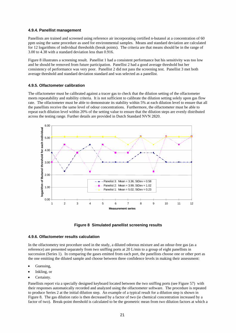
21

4.9.4. Panellist management

Panellists are trained and screened using reference air incorporating certified n-butanol at a concentration of 60 ppm using the same procedure as used for environmental samples. Means and standard deviation are calculated for 12 logarithms of individual thresholds (break points). The criteria are that means should be in the range of 3.00 to 4.38 with a standard deviation less than 0.916.

Figure 8 illustrates a screening result. Panellist 1 had a consistent performance but his sensitivity was too low and he should be removed from future participation. Panellist 2 had a good average threshold but her consistency of performance was very poor. Panellist 2 did not pass the screening test. Panellist 3 met both average threshold and standard deviation standard and was selected as a panellist.

4.9.5. Olfactometer calibration

The olfactometer must be calibrated against a tracer gas to check that the dilution setting of the olfactometer meets repeatability and stability criteria. It is not sufficient to calibrate the dilution setting solely upon gas flow rate. The olfactometer must be able to demonstrate its stability within 5% at each dilution level to ensure that all the panellists receive the same level of odour concentrations. Furthermore, the olfactometer must be able to repeat each dilution level within 20% of the setting value to ensure that the dilution steps are evenly distributed across the testing range. Further details are provided in Dutch Standard NVN 2820.

0.00

1.00

2.00

3.00

4.00

5.00

6.00

1 2 3 4 5 6 7 8 9 10 11 12

Measurement series

loga

rithm

of B

utan

ol th

resh

old

for e

ach

indi

vidu

al

Panelist 3: Mean = 3.36; StDev = 0.58Panelist 2: Mean = 3.99; StDev = 1.02Panelist 1: Mean = 5.02; StDev = 0.23

Figure 8 Simulated panellist screening results

4.9.6. Olfactometer results calculation

In the olfactometry test procedure used in the study, a diluted odorous mixture and an odour-free gas (as a reference) are presented separately from two sniffing ports at 20 L/min to a group of eight panellists in succession (Series 1). In comparing the gases emitted from each port, the panellists choose one or other port as the one emitting the diluted sample and choose between three confidence levels in making their assessment:

• Guessing, • Inkling, or • Certainty. Panellists report via a specially designed keyboard located between the two sniffing ports (see Figure 57) with their responses automatically recorded and analyzed using the olfactometer software. The procedure is repeated to produce Series 2 at the initial dilution step. An example of a typical result for a dilution step is shown in Figure 8. The gas dilution ratio is then decreased by a factor of two (ie chemical concentration increased by a factor of two). Break-point threshold is calculated to be the geometric mean from two dilution factors at which a

22

“certain and correct” result is recorded. The panellists repeat their assessments at six dilution levels, with two series at each dilution step, resulting in a total of 8x6x2 = 96 assessments (sniffings) from the eight panellists.

In Table 6, the break-point threshold is determined as the geometric mean of the lowest correctly chosen dilution ratio selected with certainty and consistency of correct choice for less dilute samples and the dilution step before it. In forced choice dynamic olfactometry, two sniffing ports are used. At each presentation, in random order, the two ports present odour-free air and diluted sample respectively to the panellist for assessment. During a panel session of about four hours, a 15 minute break is taken to minimize panellist olfactometry fatigue.

Olfactometry results may be presented either as “guess and correct” or as “certainty and correct” thresholds. Results also depend on the quality of the olfactometer, the screening of panellists, the repeatability and reproducibility of the procedure used and quality control achieved by the laboratory. Consequently it is necessary to cite olfactometry results in terms of the type of olfactometer and procedures used and to indicate whether “guess and correct” or “certainty and correct” thresholds have been calculated. Analyses of CWWT odour test data indicate that odour concentration measurements based on certainty have a lower standard deviation than one based on “guessing and correct” criteria. In the present study, the “certainty and correct” criteria were adopted.

Table 6 Odour concentration calculation demonstration

Panellist response at dilution step (number of times sample diluted)

Break-point threshold

Panellist 32 64 128 256 512 1024

1 6 6 5 3 2 2 91

2 6 6 4 3 4 4 91

3 6 3 4 3 3 1 45

4 6 6 6 4 2 1 181

5 6 3 3 4 3 1 45

6 6 5 3 3 2 2 45

7 6 6 6 4 2 1 181

Series 1

8 6 6 5 3 1 2 91

1 6 6 6 3 2 2 181

2 6 5 4 3 4 4 45

3 6 6 4 3 3 1 91

4 6 6 4 4 2 1 91

5 6 5 3 4 3 1 45

6 6 6 3 3 2 2 91

7 6 6 4 4 2 1 91

Series 2

8 6 6 6 3 1 2 181

Geometric Average (Odour Concentration) 87

In above table: 1: Guessing and wrong; 2: Guessing and correct; 3: Inkling and wrong; 4: Inkling and correct; 5: Certainty and wrong; 6: Certainty and correct

23

4.9.7. Odour emission rate calculation

The Odour Emission Rate (OER), as shown by Equation 4, can be calculated from the odour concentration as measured by the olfactometer and ventilation rates in a shed:

OCVOER ×= [ 8 ]

where

OER odour emission rate, ou/sec V ventilation rate, m3/sec OC odour concentration, ou/m3

The odour emission rate can be entered into an air dispersion model to predict the downwind odour concentration.

4.10 Odour intensity measurement To describe the concept of odour intensity, one can use the following example: odour concentration may be considered as the number of spoons of sugar added to a cup of coffee while odour intensity may be regarded as the perceived sweetness of the coffee

Odour intensity describes the relative magnitude of an odour sensation experienced by a person. Odour intensity can be expressed as an odour intensity level, which is a verbal description of an odour sensation to which a numerical value is assigned. The relationship between perceived psychological intensity and odorant concentration is suggested by Steven’s law. Stevens proposed that the perceived psychological intensity is a function of the odorant concentration (chemical concentration):

nCCkI )( 0−= [ 9 ]

where

I perceived psychological intensity K constant dependent on the choice of units of C and I C physical intensity expressed as concentration of odour compound C0 an estimate of the odour detection threshold concentration N constant which varies from 0.07 to 0.7, dimensionless

Equation 9 can be expressed as illustrated in Figure 9.

0

1

2

3

4

5

6

Odo

ur in

tens

ity Gradient n

Odour concentration Co

Chemical concentration

Figure 9 Odour intensity versus chemical concentration

Perceived psychophysical odour intensity increases as a power function of physical intensity (i.e. the concentration of odorous compound). The exponent (n) is the most important parameter that depends on the odorant. The fact that the exponent (n) is less than one indicates that if the concentration of an odour compound is halved, the perceived psychological intensity, in most situations, does not halve but rather is decreased only

24

0.7 times. Furthermore, for two different odours at the same perceived intensity, the odour with a lower (n) value is considered more pervasive and less susceptible to disappearance by dilution.

The equation 9 can be used to calculate the exponent n for a particular odorous compounds or mixture of odorous compounds. For an odour, where the chemical concentration is given as Ci, the equation can be rewritten:

nnoii DDKDCDCkI )/1/1()//( 0−=−= [ 10 ]

Where

K a constant ( nikC= ), dimensionless

D dilution ratio at the point where odour intensity is being assessed

0D Dilution ratio at the odour threshold

Equation 10 can be further rewritten as:

)/1/1()( 01 DDnLogKILog −+= [ 11 ]

Where

1K a constant ( Klog= ), dimensionless

In the equation 11, )(ILog , )/1/1( 0DDLog − can be experimentally determined using the procedure

specified in VDI 2882. Consequently for each determination, 1K and n can be calculated using a linear

regression analysis. Experimentally determined values of 1K and n are then averaged to give a representative odour intensity relationship for the poultry odour.

The procedure used by CWWT to measure odour intensity in the present study was as follows. Using the CWWT olfactometer, a portion of an odorous air sample is released from either the left sniffing port or the right sniffing port (as instructed by the operator) at a concentration higher than the odour threshold. Odour free air is also released from the other sniffing port. The panellists sniff in turn and each makes a judgment on odour intensity on the basis of the descriptors specified in Table 7. After all panellists have made their assessment, testing takes place again but at a higher odour concentration.

Table 7 Odour intensity criteria

Odour Intensity level Extremely strong 6

Very strong 5

Strong 4

Distinct 3

Weak 2

Very weak 1

Not perceptible 0

Odour intensity measurement is of particular significance in understanding perceived odour intensity where odour concentration approaches its detection threshold. When an odour is dispersed in air, the perceived odour intensity will be reduced. Initially (seconds/minutes), the odour intensity may not be perceived to reduce because of a lag in olfactometry sensation. However, with further dilutions, the perceived odour intensity will be reduced according to Stevens’ law (Equation 10) to a threshold level. Experimental work at CWWT and in Germany indicates that an odour nuisance threshold occurs when the perceived odour intensity reaches a value of 3, the level at which an odour is perceived to be distinct. At the odour detection threshold and just above the threshold, an odour will not be perceived as an offensive odour (ie one likely to cause an odour complaint). In

25

the experience of CWWT, verifiable odour complaints will arise only when residents or others experience a distinct odour in the vicinity of the odour source.

Table 8 presents an example showing how the odour intensity relationship (equation 11) has been calculated for a single odour sample. The table shows a set of typical odour intensity level responses by individual panellists to olfactometer presentations at a range of dilution steps for the sample. The average of the responses by the seven panellists for each dilution step was calculated and a regression analysis made to determine the linear relationship.

Table 8 Illustration of odour intensity measurement calculation (one sample)

Dilution step (D) Panellist Number 128 64 32 16 8 4

588 0 1 2 4 5 6

578 0 1 2 4 5 6

584 0 1 2 4 5 6

582 0 1 3 4 5 6

585 0 0 2 5 5 6

583 0 1 2 4 5 6

571 0 0 2 3 4 5

Do = 329

1/D-1/ Do 0.013 0.028 0.059 0.12 0.25

Log(1/D-1/ Do) -1.900 -1.550 -1.226 -0.914 -0.607

Average intensity (I) 0.7143 2.1429 4 4.8571 5.8571

Log(I) -0.146 0.331 0.6021 0.6864 0.7677

Log(I) = 0.684 Log(1/D-1/OC) + 1.30

For sets of samples from farms in the two states, the constants in the equation were averaged to derive an odour intensity relationship for the farms measured in each state. The dilution step (D3) at which odour was perceived as distinct was then calculated for an odour intensity level of 3 (see Table 23). The COC was calculated on the basis of averaged odour concentration for the samples and dilution step (D3).

Consequently in the study, an odour intensity level of 3 has been taken as the criterion for odour nuisance. At each of the farms studied, the olfactometry data obtained were also used to calculate the dilution ratio (D3) corresponding to an odour intensity level of 3 for a representative odour concentration inside the shed using the experimentally derived odour intensity relationship. The critical odour concentration (COC), the odour concentration corresponding to an odour intensity level of 3 without dilution, can be calculated using the following equation:

30 / DDCOC = [ 12 ]

where:

COC critical odour concentration (ou/3) D0 average odour concentration of samples tested, ou/3

D3 dilution ratio corresponding to an odour intensity level of 3 Critical odour concentration is a characteristic of a specific type of odour, but may be averaged over a set of samples. In the current study, the critical odour concentration for broiler farm odour was determined separately for New South Wales and Victorian farms to allow for the possibility of regional variation.

4.11 Odour dispersion modelling The fresh air moving past the farm will further dilute odorous gas emitted from a group of broiler sheds. Increasing wind speed and turbulence will lead to greater mixing and increased dilution. Consequently, odour

26

impact on persons in the vicinity of the farm will decrease beyond the farm. The actual odour dispersion taking place will depend primarily on the weather at the time. Weather was characterised using the well known Pasquill atmospheric stability criteria. When the outside air is still and slow moving, little mixing takes place and relatively high odour concentrations may be maintained at some distance away from the farm. Well established air dispersion modelling techniques are available to estimate the odour concentration including odorous gases, at a distance from a source.

Air dispersion models may be used to predict the odour concentration that would result from an odour pollution source, for any specified meteorological conditions, at any location, for any time period. The models mathematically simulate odour dispersion processes in the atmosphere and provide a relationship between the odours generated at a source and the downwind odour concentrations in the atmosphere experienced by a receptor. As with other gases, odour dispersion may be modelled using available dispersion models such as Ausplume, ISC3 and puff models such as Auspuff. ISC3 was developed in the United States and is widely, although not exclusively, used throughout the world. Ausplume has been used extensively for regulatory air quality impact analyses in Australia and New Zealand for almost 20 years. Auspuff is an upgraded modelling system that offers many advantages and capabilities such as the use of three-dimensional meteorological data. Instead of assuming that the concentration profile within a plume is evenly distributed, a Puff model evaluates the contribution of an instantaneous puff in the atmosphere over a given period such as one hour. Puff models have only recently moved beyond use solely for research and development applications.

In the current study, Ausplume (4th version) has been applied to all farms studied because of its accessibility. The structure of the model is outlined in Lorimer, 1986. At some farms, it has also been possible to apply Auspuff, although the meteorological data sets used have proved to be somewhat deficient because of the absence of appropriately configured weather stations in close proximity to the farms studied. However, given the installation of the project funded weather station at Farm NB in April 1998, it is expected that sufficient data to enable a more adequate comparison of Auspuff with Ausplume will be available by April 1999.

Ausplume is a Gaussian plume model, which assumes that elevated plumes from a continuous and elevated point source have a Gaussian (or normal) distribution of mean concentration. The assumption is strictly applicable, only in the case of stationary, homogeneous turbulence in the atmosphere. For further details see Lorimer (1986).

The Gaussian plume equation can be expressed as:

)2

exp()2

exp(2

);,,( 2

2

2

2

zyzy

zyu

QtzyxCσσσσπ

−⋅−⋅⋅⋅⋅

= [ 13 ]

where:

);,,( tzyxC concentration at point (x,y,z) averaged over time t x: distance downwind from the sources at a position of (0,0,0) y distance across-wind z height within the plume Q emission rate u wind speed

yσ and zσ dispersion coefficients representing crosswind and vertical spread, which are increasing functions of x and t

In Equation 13, the emission rate Q and dispersion coefficients yσ and zσ are the critical factors in determining

downwind concentrations. In practice, it is very difficult to determine the emission rate continuously over a period of time. As a consequence for the purposes of modelling, a worst case scenario was developed to

represent a whole year. (See Section 5.11.1 below.) The dispersion coefficients yσ and zσ were derived from

field observations and theoretical calculations (Seinfeld, 1986).

Odour dispersion modelling using Ausplume requires several inputs, including odour emission rates, source characteristics, receptor locations, terrain effects and meteorological data. The model calculates the hourly concentrations for each hour of the meteorological data set for a selected grid of receptor locations. Finally, the results are stored and sorted in ascending order for each receptor. For the current study, interpolating between

27

grid points then plots isopleths of odour dispersion based on the 44th highest hourly averaged odour concentration level for a year at each receptor point (ie at the 99.5th percentile).

The assumptions adopted in the study for dispersion modelling are discussed in the following sections.

4.11.1 Odour emission rates

The characterisation of the pattern of odour emission rates during a year requires the adoption of simplifying assumptions to produce an algorithm to use in the dispersion modelling process. Ausplume and Auspuff make provision for a number of ways to characterise odour emission rates over a time period. Options available allow for consideration of aspects such as:

• A constant emission rate • By hour of day • By hour and season • By month • By wind speed and stability category and • By ambient temperature The odour emission rates from a broiler shed are highly variable through a year. Usually there are 5 to 6 growout batches each year. Within each growout batch, it has been assumed that average odour concentrations in sheds gradually increase to a plateau at about Week 6. Ventilation rates will frequently vary in response to changing ambient temperature. In conditions of low ambient temperature (eg 15 °C and below), sheds are frequently operated in minimum ventilation mode. From observation of farm operations and ventilation measurement results in the study, Table 9 has been developed for use in dispersion model calculations in the study. Studies undertaken in Europe (O’Neill et al. 1992) based on consideration of heat removal at various bird weights and solar gain, confirmed that the values used in Table 9 provide a realistic basis for odour assessment modelling.

Table 9 Assumed odour emission rates as a function of ambient temperature used in Ausplume modelling

Temperature (°C) 0 5 10 15 20 25 30 35 40

Percentage of maximum emission rate assumed 10 10 10 10 100 100 100 100 100

4.11.2 Averaging time

It is important to indicate that for any averaging time less than one hour, a scaling factor based on Equation 14 must be applied to δy:

2.000 )/(),( ttttf = [ 14 ]

For instance, if three minutes average data is used, the scaling factor from hourly data will be 1.8. This will be

applied in the estimation of dispersion coefficient yσ. Although a number of algorithms are used to fine tune

the dispersion Equation 13, predicted three minute odour concentrations will be approximately 1.8 times larger than sixty minute odour concentrations. Theoretically, dispersion coefficients are based on values averaged over ten minutes while in most cases meteorological data is presented as one hour averaged values. Use of ten minute averaged meteorological data is possible but the additional computation required is seldom justified. However, in some situations an alternative to Ausplume using ten minute data may prove cost effective. There appear to be no technical advantages in using a three minute averaging time rather than a one hour averaging time.

4.11.3 Source characteristics

Broiler sheds vary by type. They may be naturally ventilated, cross-flow and/or tunnel ventilated. Tunnel ventilated sheds may be configured to operate in minimum ventilation mode. For modelling purposes, naturally ventilated and cross-flow sheds can be treated as typical volume sources.

28

Hx Fan

X

Vi Vx

Wx

Figure 10 Illustration of odour plume from a tunnel ventilated shed

For a tunnel ventilated shed operating in tunnel ventilation mode, the whole shed is under negative pressure relative to atmosphere. Exhausts may be vented horizontally by a series of fans at one end of the shed. A shed operating in this mode can be regarded as a series jets emitting exhaust air into a free space (See Figure 10). The actual plume is in filler space with a conical shape. To model the plume, a rectangle can be assumed. The angles of divergence range from 20° - 24° with an average of 22°. (ASHRAE, 1997). Coalescing jets expand at smaller angles averaging 18°.

The distance can be estimated using the following equations (ASHRAE, 1997):

fadcx RCAVQKX'

= [ 15 ]

where

X distance from outlet to measurement of centreline velocity xV , m 'K centreline velocity constant depending on outlet type and discharge pattern

Q discharge flow rate from outlet, m3/s

xV centreline velocity at distance X , m/s

cA measured gross area of outlet, m2

dC discharge coefficient (usually between 0.65 – 0.9)

faR ratio of free area to gross area

29

In equation 15, the 'K constant is 7. The dC value is 0.7. The xV value can be calculated from the meteorological data used in the dispersion model and the wind profile equation to convert the wind speed at a 10 metre height to a 2 metre height which is the centre line of the plume. If a typical value of 2 m/s is used, the plume length will be about 25 metres.

The actual horizontal and vertical spread of the plume will be larger than the width and height of the shed if all the fans are operating. However, to be conservative, the width of the plume is assumed to be the same as the width of the shed and the height of the plume is taken as the side height for single row or ridge height for a multiple row shed.

4.11.4 Receptor locations

A grid of 2000 m x 2000 m with a spacing of 50 m was used for all dispersion modelling in the study. The grid so created results in 41 x 41 receptors assumed to be located around the farm.

4.11.5 Meteorological data

The meteorological data used to characterise weather conditions included time and day, temperature, wind speed, wind direction, atmospheric stability, mixing depth and sigma-theta (σθ) values. Where available, meteorological parameters such as ambient temperature at various heights, and solar and net radiation were used to calculate mixing height and stability class.

4.11.6 Limitations of Ausplume for modelling odour generated by broiler farms

Ausplume dispersion modelling provides the key to benchmarkng between farms using available odour measurement data. Ausplume may be used to predict 99.5th percentile highest hourly averaged odour concentrations in the neighbourhood surrounding a farm and to define an odour impact area. Community surveys may be used to validate the results based on dispersion modelling.

Modelling cannot be used to predict specific individual cases of odour complaint, but may be used to define an odour impact area indicating the relative likelihood of complaints between farms employing various practices in planing and management.

Dispersion modelling provides a conservative prediction based on the worst case situation for the source emission data. In a real situation, the odour emission rates from a shed will generally increase through a growout cycle, reaching a plateau at about Week 6. Taking account of the growth cycle and periods between batches, maximum odour emission can be expected to occur during only about 20% of the days in a year. Modelling does however account for the variation in atmospheric conditions through a year that drive the extent of dispersion and dilution of odour as it moves away from the farm.

4.12 Development of odour impact criteria Odour impact criteria are parameters including odour concentration, exceedance probability, averaging time and receptor location used to provide objective means for defining odour impact area in which perceived odour likely exceeds distinct level for a limited time in a year. An odour impact area around a source, such as a group of broiler growout sheds, may be defined using air dispersion modelling together with an odour impact criteria appropriate to the land uses surrounding the farm. Within a defined odour impact area, typical receptors (e.g. residents) can be expected to perceive the odour as distinct or strong. Odour impact criteria are not ambient odour standards but rather provide a scientifically derived benchmark for the making of informed decisions in planning, design, environmental management and regulation.

Many environmental managers and environmental regulatory agencies use air dispersion models and odour impact limits to estimate odour impact from the broiler farms. Table 10 lists some typical odour impact limits used in several jurisdictions in Australia and overseas. Care must be taken when using figures based on the various configurations of olfactometers used in the past. With the introduction of the Australian and European standards for the undertaking of odour concentration measurement using dynamic olfactometry, it could be expected that many of the limits quoted in Table 10 would be incompatible with current practice.

Table 10 Some odour impact limits used in several jurisdictions

30

Jurisdiction Odour concentration

(ou/m3)

Exceedance probability (Percentile)

Averaging time

Receptor location

Source

New South Wales, Australia

2 99.5th percentile

3 minutes Resident CASANZ 1995

Queensland, Australia

10 99.5th percentile

1 hour Resident Verrall, 1997, EPA Qld 1999

Victoria, Australia 1 99.9th percentile

3 minutes Resident CASANZ, 1995

The Netherlands (new installations)

1 99.5th percentile

1 hour Domestic dwelling

Hermia and Vigneron 1994.

Denmark 5-10 0.6-20

99th percentile

1 minute 1 hour

Plant surroundings

Boholt 1992

New Zealand 2 99.5th percentile

1 hour Property boundary

Ministry for Environment, New Zealand 1995

Massachusetts, USA

5 Highest 1 hour Plant boundary

Mahin, 1997

As shown in Table 10, a wide range of odour impact limits have been reported and the question could be asked as to why there is so much variation. One reason is that during recent years, modern performance based forced choice dynamic olfactometry has greatly improved the sensitivity of odour measurement but as yet not all the values are based on such measurement. For instance, the butanol threshold measured using a three port IITRI (Illinios Industrial Triangle Research Institute) olfactometer, ranged from 80 - 200 ppb while modern dynamic olfactometry is capable of measuring butanol threshold levels from 20 to 80 ppb. Assuming that the same sensitivity applies to environmental odour samples, comparable odour impact thresholds could be 3 - 20 times lower. Correspondingly, a nuisance threshold that was determined as 1 ou/m3 using the less sensitive earlier equipment could be rated at 3 - 20 ou/m3 using modern equipment. In summary, the use of advanced olfactometer based methods could result in nominally much higher odour concentration limits being specified in odour impact criteria for no substantive change in actual impact on receptors.

A variety of approaches to odour measurement and regulation have been adopted around Australia. Although the control of broiler farm odour is primarily a matter for local government councils, the councils are subject to State legislation. State environment protection agencies generally provide scientific and professional support for odour control by councils.

Odour management for broiler farms has been the focus of much attention in regions of Victoria where poultry growing takes place in areas of increasing population and land prices (Ainsworth 1992). In the Mornington Peninsular Shire (1996), locational and buffer criteria are set for broiler farms.

The framework for regulation of odour in Victoria is provided by the State Environment Protection Policy (The air environment) - SEPP Air CASANZ(1995) and Buchanan (1997). A 1982 amendment to SEPP Air provided that: “a design ground level concentration of one odour unit may be applied”. The legislation led to the development and adoption of what was then a state of the art method of odour measurement (Method B2). Since that time the conceptual basis of odour assessment and measurement methodology have been subject to much refinement. Consequently, the basic method of measurement currently used in Victoria, while particularly advanced at the time of its introduction, cannot approach the sensitivity of detection and repeatability achieved using modern dynamic olfactometry and internationally standardised procedures such as those developed and currently used in Europe. As summarised by Buchanan (1997) the main emphasis of the EPA “is on preventative measures including the implementation of cleaner production and waste minimisation, good land-use planning with appropriate buffer distances, and a design ground level concentration of 1 odour unit.”

31

New South Wales regulatory arrangements for odour are outlined in CASANZ (1995). Local government councils in areas in which broiler farming is undertaken, may promulgate planning and development control instruments in which odour management is a primary focus. (Cessnock City Council 1994, Lismore City Council 1994, Wollondilly Shire Council 1995). A workgroup was set up to develop a new guideline for agriculture and is progressing.

Provision has been made under Section 129 and Schedule 1 of the New South Wales Protection of the Environment Operations Act 1997, for the licensing of the emission of odours from large broiler farms in New South Wales. The Authorised officers manual on odour control, (EPA, NSW 1998) supplies technical information on how odours are measured and how odours are governed by the Clean Air Act 1961. The manual outlines procedures consistent with those used in the current study for both odour measurement and impact assessment. In NSW, in situations where odour dispersion modelling is required, an odour impact criteria of a 3 minute averaged concentration of 2 ou/m3 at the 99.5th percentile has been adopted.

An outline of odour regulatory measures in Queensland was presented in CASANZ(1995). Verrall (1997) has presented a recent outline of odour policy in Queensland. Currently used transitional odour assessment criteria used in relation to new developments, are based on the use of modern dynamic olfactometry and odour dispersion modelling using Ausplume. However, Queensland is giving consideration to non-specific community odour annoyance criteria (eg 5 % of a population experiencing annoyance for less than 2% of the time). Following a technical review and workshop, a one hour averaged odour design goal of 10 ou/m3, not to be exceeded more than 0.5% of the hours in one year, has been suggested. (Verrall 1997)

Under the Environment Protection Act 1993 of South Australia, all people have a general duty to minimise environmental harm. Compliance with the document, Guidelines for the establishment and operation of broiler farms in South Australia, March 1998 (EPA, SA 1998) “will generally mean meeting the requirements to minimise environmental harm”.

Regulatory arrangements and current developments for odour management in Western Australia are outlined in CASANZ (1995) and Pitt (1997). A Western Australia odour policy involving consultation with industry and other interested stakeholders is currently being developed. Odour design criteria in use internationally and nationally are being evaluated by the WA Department of Environmental Protection through a study of emission rates and dispersion modelling for selected broiler farms for which complaint details are known. The Department considered that it would be particularly useful to develop a model to determine the extent of buffer distances upon application of relevant odour standards/guidelines. (Vogel 1995(a)) In parallel, the WA Planning Commission has established a Poultry Farm Relocation Working Group to address strategic issues relating to broiler farms and future urban development. Work undertaken by CWWT in 1997 on broiler and egg production broiler farms in WA using methodology similar to that used in the current study is contributing to the further development of the WA approach.

4.13 Community survey A community survey was undertaken over one growout batch at farm NA during the first quarter of 1997. Sixteen individuals in fifteen households took part in the survey. The survey uses the methodology set out in German Standard VDI 3883. The results of the community survey taken, together with the results of the odour intensity studies, provided the basis for establishing odour impact criteria for broiler farms. Details of letters and forms used in the survey are set out in Appendix 6.

The participants of the survey are required to make a daily odour assessment outside their house between 6:00 – 8:00 pm and recorded their responses ( 0 – 5 scales similar to Table 7 without the highest scale, extreme strong) on a standard form. Further information about the characteristics of the odour were also required if they perceived odour as above distinct.

32

5. Detailed Results As a first step, sampling and measurement protocols for the studies, including location of sampling points within sheds, were experimentally checked under typical batch conditions and the protocols finalised. To the extent possible, temperature and humidity were measured at each farm throughout the period of study of the farm. At the start of the full year emission study on two New South Wales farms, ammonia concentration within sheds and at the litter surface was measured. At the same time, ventilation rates of sheds were continuously monitored using an anemometer transducer. Because of the high cost and to achieve maximum cost effectiveness, the timing of odour sampling and measurement was carefully planned taking into account the results of ammonia and other environmental monitoring results.

Planning for the spot emission survey drew heavily on the results and experience of the two farm study. Odour sampling and testing for the spot emission survey was undertaken during week 6 of batches to capture data covering the period of peak odour emission. Study results are presented in the remainder of the section. The course of the study was conditioned by the problems encountered in the broiler shed environment and the intermediate results obtained during the progress of the field work. Some explanation is provided to show how the results were obtained and to document field conditions during sampling and measurement. Table 11 shows the convention adopted linking batch stage in weeks to bird age in days.

Table 11 Convention adopted linking batch stage in weeks to bird age in days

Bird age in days 1 – 7 8 - 14 15 - 21 22 - 27 28 - 35 36 - 42 43 – 49 49 - 56

Week of Batch 1 2 3 4 5 6 7 8

5.1 Temperature and Humidity Temperature control of the birds is the critical environmental factor in broiler growth. shows a typical air temperature profile for a broiler growout batch. As shown in, temperature and humidity were measured inside a shed at Farm NB during a 17 day period in March 1998 in order to observe typical day by day variation.

Data presented in Figure 11 were recorded every minute. The upper chart depicts temperature and humidity recorded at the high position which is just below the ridge opening. The lower chart depicts the temperature and humidity recorded at a height of 50 cm, just above the birds.

0

20

40

60

80

100Humidity Temperature

0

20

40

60

80

100Humidity Temperature Lower flap opening

Upper flap opening

Figure 11 Temperature and humidity inside shed at Farm NB over 17 days

33

5.2 Ammonia concentration at different positions inside a shed Ammonia levels were measured using wet chemistry. An attempt to use an automatic sensor attached to a weather station data logger proved unsuccessful because of instability in the sensor, its signal transfer and breakdown of the station computer, apparently induced by shed dust and/or humidity.

Results for ammonia concentrations measured at different locations along a shed during the first batch studied at Farm NA are shown in Figure 12. Ammonia concentration, as measured inside the shed on nine days, is plotted relative to the sampling points (position along the length of the shed and sampling height) as shown on the x-axis. The measurements were made during the period, 13 February – 5 March 1997 at a bird age of 3 – 5 weeks.

0

2

4

6

8

10

12

14

1/4L@1m 1/4L@2m 1/2L@1m 1/2L@2m 3/4L@1m 3/4L@2m

Sampling locations

Am

mon

ia c

once

ntra

tion,

ppm

Figure 12 Ammonia concentration at different locations along a shed on nine days

5.3 Ammonia concentration in a single batch Figure 13 shows the averaged results of ammonia concentration determinations in a representative shed during four batches at Farm NA and NB during periods shown Table 12. Plots of ammonia concentration are shown in Figure 13. Ammonia concentration was measured four times in the morning of each sampling day and daily and weekly averages computed.

Table 12 Schedule of ammonia sampling

Farm Abb. Date Comments Farm NA Batch 1 FNAB1 Jan – Mar 1997 1 - 3 days/week, pick-up at week 5

Farm NA Batch 2 FNAB2 Feb – Mar 1998 1 - 3 days/week. pick-up at week 6

Farm NB Batch 1 FNBB1 Jan –Feb 1997 Weekly sampling no pick-up

Farm NB Batch 2 FNBB2 Mar 1998 Weekly sampling no pick-up

34

.

0

5

10

15

1 2 3 4 5 6 7 8

Bird age, weeks

Am

mon

ia c

once

ntra

tion,

ppm

FNAB1 FNAB2 FNBB1 FNBB2

Figure 13 Ammonia concentration in shed for several batches at Farms NA and NB

Figure 14 and Figure 15 show the data of Figure 13 recalculated in relation to bird weight. Bird weight was calculated by counting, sampling and weighing individual birds.

0

1

2

3

4

5

6

7

8

9

1 2 3 4 5 6 7

Bird age, week

Am

mon

ia c

once

ntra

tion,

ppm

0

5000

10000

15000

20000

25000

30000

35000

40000

45000

Bird

wei

ght,

Kgs

ammonia concentration Bird weight

Figure 14 Ammonia concentration and bird weight at Farm NB

35

0

2

4

6

8

10

12

14

16

18

20

1 2 3 4 5 6

Bird age, week

Amm

onia

con

cent

ratio

n, p

pm

0

5

10

15

20

25

30

35

40

Bird

wei

ght,

1000

kg

Ammonia concentration] Standard bird weight Actual bird weight

Figure 15 Ammonia concentration and bird weight at Farm NA

5.4 Ammonia concentration from litter surface Parallel measurements of ammonia concentration were also taken at the litter surface at Farms NA and NB using a wind tunnel system at the time of the ammonia concentration measurement shown in Figure 13 - Figure 15. Results are presented in Figure 16.

0

2

4

6

8

10

12

14

16

1 2 3 4 5 6 7 8

Bird age, weeks

Am

mon

ia c

once

ntra

tion,

ppm

FNAB2 FNBB2

Figure 16 Ammonia concentration at litter surface for batches at Farm NA

36

5.5 Litter moisture A comparison of measured odour concentrations at six New South Wales farms with litter moisture measurements taken at the time of sampling is shown in Figure 17.

0

200

400

600

800

1000

1200

NV NB NA (2) NS NV NA NCFarms

Odo

ur c

once

ntra

tion,

ou/

m3

0

10

20

30

40

50

60

Litt

er m

oist

ure

cont

ent,

%

Odour concentration Moisture

Figure 17 Odour concentration and litter moisture at NSW farms

A comparison of measured odour concentrations at six Victorian farms with litter moisture measurements taken at the time of sampling is shown in Figure 18.

0

100

200

300

400

500

600

700

800

900

1000

VE1 VD VA VC VE2 VB

Farms

Odo

ur c

once

ntra

tion,

ou/

m3

0

10

20

30

40

50

60

Litt

er m

ositu

re c

onte

nt, %

Odour conc. Moisture

Figure 18 Odour concentration and litter moisture at Victorian farms

37

5.6 Feed trial Following each day of sampling, samples were transported to Weston Food Laboratories for Kjedahl Nitrogen analysis within 24 hours of sampling. Analysis used the semi-automated Kjeltec method. Kjedahl Nitrogen results are set out in Table 13.

Table 13 Kjedahl Nitrogen results

Kjedahl Nitrogen (% dry weight)

litter fresh faeces

Bird age (days)

A B C A B C

21 4.5 3 4.6 3.4 4.2 2.9

28 4.6 5.6 5 4.4 5.3 5.2

35 4.2 4.3 6 4.2 6.1 5.1

42 6.9 3.9 3.3 6.9 5.9 3.9

N.B. A: low protein feed; B: standard feed; C: high protein feed

Results from measurement of ammonia emission from the pen litter are listed in Table 14.

Table 14 Ammonia concentration at litter surface

Ammonia Concentration (ppm)

14 days 28 days 35 days 42 days

A B C A B C A B C A B C

0.44 0.75 0.44 1.67 1.49 2.2 2.68 2.5 2.06 4.66 3.47 3.87

0.53 0.66 0.83 1.54 1.98 1.89 3.16 2.85 1.54 5.67 5.93 4.83

0.4 0.4 0.61 1.71 2.15 1.93 3.03 N/A 2.72 5.53 5.18 6.19

0.53 0.53 1.05 2.28 1.8 1.27 3.38 2.37 3.91 4.79 5.93 5.67

0.88 0.48 0.48 1.23 1.27 1.84 2.72 3.56 3.12 3.91 5.31 5.89

0.7 0.4 0.7 1.58 1.19 2.02 2.42 2.59 2.33 3.34 N/A 4.79

0.97 0.79 0.75 N/A 2.11 2.06 2.9 2.55 2.11 5.62 4.92 3.82

0.75 0.92 0.79 1.63 1.63 1.23 2.15 2.72 3.07 5.18 5.8 5.62

5.7 GC-MS results A total of four samples (Sample 1 to Sample 4) were taken from a shed at Farm NB on March 2 1997 and sent to ANSTO for GC-MS analysis. The analytical method is detailed in Section 0. Later, another four samples (Samples 5 to 8) were collected in canister cylinders at Farm NG2 and sent to NZ for analysis. Table 15 lists the major compounds determined from the four samples. GC-MS Chromatograms are listed in Appendix 5.

5.8 Farm survey results Field data was collected over the period February 1997 to March 1998. During the year, twenty-two odour samples were taken at Farm NA and subjected to olfactometry testing for measurement of odour concentration and/or odour intensity. At Farm NA, nine samples were taken across the autumn of 1997, four during the winter of 1997, six during the summer of 1997-98 and three in the autumn of 1998. During the same period, twelve odour samples from Farm NB were tested. At Farm NB, three samples were taken in the winter of 1997, three in summer of 1998-89 and six in the autumn of 1998. Farms NC, ND and NE were tested in the summer of 1997-98 and Farm NF tested in autumn 1998.

Figure 19 shows the results for measurements of odour concentration on samples taken at the eight New South Wales farms studied.

38

Table 15 Major compounds determined by GC-MS analysis Unit: ppb

Compounds Odour threshold

ppb

Sample 1

Farm NB

Sample 2 Farm NB

Sample 3 Farm NB

Sample 4 Farm NB

Sample 5 Farm NG2

Sample 6 Farm NG2

Sample 7 Farm NB

Sample 8

Farm NB

Methylmercaptan 1.1 N/A N/A 4.75 3.67 N/D N/D N/D N/D

Ethylmercaptan 0.19 0.05 0.03 N/A N/A N/D N/D N/D N/D

Propylmercaptan 0.5 0.02 0.01 <0.03 <0.03 N/D N/D N/D N/D

Carbonylsulfide - 11.14 8.00 0.6 0.59 N/D N/D N/D N/D

Carbondisulfide 210 5.89 4.75 0.22 0.18 N/D N/D N/D N/D

Dimethyl sulfide 1 1.86 1.72 0.34 0.3 N/D N/D 3.99 0.798

Dimethyl disulfide 0.7 1.63 2.04 2.12 0.99 6.02 27.37 36 21.3

Dimethyl trisulphide

1.3 N/A N/A N/A N/A 0.05 0.28 1.92 1.37

Acetaldehyde 67 19.38 12.62 0.81 1.43 N/D N/D N/D N/D

Methanol 105 62.81 45.98 71.88 54.81 N/D N/D N/D N/D

Ethanol 2 30.65 31.59 31.34 31.11 N/D N/D N/D N/D

i-propanol - 4.09 8.01 2.62 2.2 N/D N/D N/D N/D

Acetone 105 36.65 40.42 12 10.95 N/D N/D N/D N/D

2-butanone - 6.83 12.22 1.78 1.74 N/D N/D N/D N/D

Acetic acid 1000 N/A N/A N/A N/A 0.18 1.71 19 5.37

Butyric acid 0.28 N/A N/A N/A N/A 0.09 0.04 1.01 N/d

Indole 0.1 N/A N/A N/A N/A 0 0.001 0.0151 0.00507

Skatole 0.075 N/A N/A N/A N/A 0 0 0.00164 0.000667

0

200

400

600

800

1000

1200

0 5 10 15 20 25 30 35 40 45 50 55 60

Sample numbers

Odo

ur c

once

ntra

tion,

ou/

m3

NA NB NC ND NE NF NG1 NG2

Figure 19 Odour concentration in sheds at eight farms in NSW

39

Results for measurement of odour concentration on samples taken at the five Victorian farms studied are shown in Figure 20.

0

200

400

600

800

1000

1200

0 5 10 15 20 25 30 35 40

Sample numbers

Odo

ur c

once

ntra

tion,

ou/

m3

VA VB VC VD VE

Figure 20 Odour concentration in shed at five farms in Victoria

5.9 Odour concentration inside sheds in relation to season Anecdotal evidence suggests that odour problems are more likely to occur at a particular season in particular locations and climatic situations. (Climate also influences shed operation and dispersion characteristics, both factor affecting odour concentrations experienced by residents in the neighbourhood of a farm.) Figure 21 presents data for measured odour concentration on samples from eight NSW farms in relation to season. The data is presented to show mean values (dots) and the spread from minimum to maximum values (upper and low bars) for each season.

0

200

400

600

800

1000

1200

Summer Autumn Winter Spring

Season

Odo

ur c

once

ntra

tion,

ou/

m3

Figure 21 Odour concentration related to season at two NSW farms

40

5.10 Ventilation rate for naturally ventilated shed The ventilation rate from a naturally ventilated shed can be determined by measuring the air velocity leaving the shed and the cross-sectional area at the point where the measurement is taken. The distribution of air velocity along the shed length was studied by placing two sensors along the downwind side of the shed at the same height but 30 metres apart from each other. A typical air velocity measurement, taken over two days on a natural ventilated shed at Farm NA, is shown in Figure 22.

For a double flap shed at Farm NB, velocity transducers were installed downwind at the upper and lower flap openings. Exit air velocity measurements, taken over seventeen days at Farm NB are shown in Figure 23 with hourly averages plotted in Figure 24.

0

0.5

1

1.5

2

13:12 16:22 19:40 22:57 2:14 5:31 11:59 15:27 18:59 22:31 2:04 5:36 9:03

Velc

oity

, m/s

0

0.5

1

1.5

2

13:12 16:22 19:40 22:57 2:14 5:31 11:59 15:27 18:59 22:31 2:04 5:36 9:03Time, min.

Velo

city

, m/s

Position 1

Figure 22 Typical air velocity over two days at Farm NA at side openings

0

0.2

0.4

0.6

0.8

1

1.2

Velc

oity

, m/s

0

0.2

0.4

0.6

0.8

1

1.2

Days

Velo

city

, m/s

Lower flap opening

Upper flap opening

Figure 23 Air velocity at Farm NB over 17 days

41

The hourly averaged exit air velocity at the upper flap was computed from data recorded at intervals of one minute. In calculating the ventilation rate, the velocity at the upper flap was used as the velocity measured at lower flap was at about the sensitivity of the velocity transducer (ie 0.1 m/s). The maximum exit air velocity during each day (0:00 – 24:00) was established by inspection and the values averaged to calculate ventilation rate.

0

0.1

0.2

0.3

0.4

0.5

Time, days

Velo

city

, m/s

Velcoity high Velocity low

Figure 24 Hourly average at Farm NB over 17 days

Velocity transducers were placed near the ridge opening and at an upper flap in a ridged shed with double flaps at Farm VA. Results are shown in Figure 25. The upper figure shows averaged values based on data recorded at intervals of one minute. The bottom figure shows hourly average values. The ventilation rates were calculated from the velocity recorded from flapper. It was noticed that the velocity recorded at the ridge was not changed a great degree. During the day, the ridge opening might become an inlet for the shed to take fresh air.

For a natural ventilated shed with a ridge, such as Victoria Farm VC, a curtain shed with a ridge opening, both air velocities were measured and their results are shown in Figure 26. The upper trace shows averaged values based on data recorded at intervals of one minute with the lower trace showing hourly averaged values. It is not clear whether the ridge opening is drawing in air or exhausting air. Consequently in calculating ventilation rates, air flow through the ridge opening was ignored.

0

0.5

1

1.5

2

2.5

Time, minutes

Velo

city

, m/s

Velocity high Velocity low

0.00

0.25

0.50

0.75

1.00

1.25

14 18 22 2 6 10 14 18 22 2 6 10 14 18 22 2 6

Time, hours

Velo

city

, m/s

Averaged over one hour

Averaged over one minute

Figure 25 Air velocity at Farm NA

42

0

0.5

1

1.5

Time, minutes

Velc

oity

, m/s

Velocity high Velocity low Averaged over one minute

0.0

0.5

1.0

1.5

15 17 19 21 23 1 3 5 7 9 11 13 15 17 19 21 23 1 3 5 7 9 11 13

Time, hours

Velo

city

, m/s

Averaged over one hour

Figure 26 Air velocity at Farm VC

A summary of ventilation rates and air exchange rates as estimated for the natural ventilated sheds studied is presented in Table 16.

Table 16 Summary of ventilation rates from naturally ventilated sheds

Farm Shed number

Number of birds

Volume Velocity Opening area

Ventilation rate

Air exchange rate

- - m3 m/s m2 m3/hr times/hr

Farm NA 2 19500 3749 0.73 28 73584 19.6

Farm NB 1 24000 4104 0.35 54 68040 16.6

Farm VC 2 30355 4453 0.46 63.9 105818 23.8

5.11 Ventilation rate for tunnel ventilated shed For a tunnel ventilated shed operating in tunnel ventilation mode, the ventilation rate can be estimated from the number of fans in operation. A field measurement at Victorian Farm VD in an empty shed is shown in Figure 27. A velocity measurement plane was selected just 10 metres away from the fan inside the shed. At the beginning of the experiment, a single fan was switched on. A hand-held anemometer with a data store function was used to take air velocity measurements at points selected by dividing the plane into 27 sections: 3 in vertical and 9 in horizontal positions. Velocities were taken at the middle of the section and the average value recorded. Then, two fans were switched on and air velocities at the plane taken again. The procedure was repeated until all 12 fans were in operation. At such times the shed opening at the other end of the shed was opened to the extent required to achieve optimal velocity across the birds.

The ventilation rate from the shed was calculated by multiplying the measured average air velocity at the velocity measurement plane by the cross sectional area of the shed at the measurement plane.

The ventilation rate for the cross flow ventilated shed studied was determined on the basis of the effective cross sectional area of the side curtain opening and air velocity measurements taken across the effective opening plane as for tunnel ventilation sheds.

43

Ventilation rates of mechanically ventilated sheds measured on Victorian farms are presented in Table 17. At the time of odour measurement, the mechanically ventilated sheds were operated at or near their full capacity.

y = 0.1191x R2 = 0.9813

0

0.2

0.4

0.6

0.8

1

1.2

1.4

1.6

0 1 2 3 4 5 6 7 8 9 10 11 12

Number of fans in operation

Velo

city

at t

he c

ross

-sec

tion

of s

hed

Figure 27 Correlation between measured air velocity at shed cross-section area against number of fans in operation

Table 17 Summary of ventilation rates from mechanically ventilated shed

Farm Shed number

Number of birds

Volume Fans on during odour

sampling

Percentage

maximum fans

Cross section

Velocity Ventilation rate

Air exchange

rate

- - m3 - % m2 m/s m3/hr times/hr

Farm VA 2 50000 8081 10 71 63.1 1.23 279562 34.6

Farm VB* 3 27500 4063 10 80 5.4 4.9 95513 23.5

Farm VD 2 43047 6684 9 75 53.9 1.19 230908 34.5

Farm VE 6 40000 7910 - - 59.5 1.2 256932 32.5

* cross flow

44

5.12 Odour dispersion modelling results The latest version of Ausplume (4.0) was used in the study. In modelling dispersion of odour from broiler farms, the set of sheds on each farm was considered as a volume source.

Table 18 Summary of meteorological data at the studied farms

Site Year Meteorological site

Distance Km

Sigma-theta

Farm NA 1998 On farm 0 No

Farm NB 1996 Bringelly 20 Yes

Farm VA 1995 Geelong 7 Yes

Farm VB 1995 Dandenong 20 Yes

Farm VC 1995 Dandenong 15 Yes

Farm VD 1995 Dandenong 10 Yes

Farm VE 1995 Bendigo 5 Yes

It should be noted that the Ausplume model is unable to allow for simulation of odour emission rate on the basis of bird age and operational pattern in modelling odour dispersion from a broiler farm. The approach adopted in the study was to simulate odour emission rate using the measured assumed worst case (Week 6) maximum odour concentration from a batch with the maximum measured and calculated daily ventilation rate. However as Ausplume is capable of allowing for variation in ambient temperature, it was possible to allow for variation of emission rate with ambient temperature (See Table 9 ).

Summaries of the sources of the meteorological information used in the study are provided in Table 18.

Source data relating to odour emission rates used in dispersion modelling for Farms NA and NB in New South Wales and Farms VA, VB, VC, VD and VE in Victoria are presented in Table 19.

Table 19 Estimated maximum odour emission rates used in modelling

Farm Farm size *

Volume of shed (m3)

Air exchange rate (times/hr)

Odour concentration

(ou/m3)

Maximumodour emission rate

(ou/s)

NA 19500 3749 19.6 297 6071

NB 24000 4104 16.6 409 7730

VA 50000 8081 34.6 373 28966

VB 27500 6684 23.5 491 13027

VC 30355 4453 23.8 418 12287

VD 43047 6684 34.5 324 20781

VE 40000 7910 32.5 290 20712

* Number of birds placed at start of batch

In dispersion model calculation, the following assumptions were made:

• Estimated maximum odour emission rate when ambient temperature above 15 °C and 10% of the maximum rate when ambient temperature at or below 15°C (See Table 9 for model settings.)

• Grid of 2 km x 2 km at 50 metres spacing • No terrain effects • One hour averaging time • Flat rural (roughness height = 0.1 metre) for land use category

45

• Sigma-theta was used for horizontal dispersion curve where available from local meteorological data and Pasquill-Gifford method was used for the vertical dispersion curve

• For tunnel ventilated sheds, the odour plume was assumed to travel about 25 metres assuming an average ambient wind speed of 2 m/s.

Seven types of farms were modelled with general conditions as set out in Table 20.

After running the Ausplume program, a subsidiary program was used to produce a table of highest concentrations at the 99.5th percentile for each grid point leading to the drawing of isopleths of concentration for that percentile. Odour concentration isopleths for the 99.5th percentile for farms for which dispersion modelling was undertaken follow.

Table 20 Summary of farm conditions

Farm Number of sheds Number of birds Shed type

NA 3 58500 Natural

NB 3 72000 Natural VA 4 143300 3 natural and 1 tunnel ventilated

VB 3 62000 Cross flow

VC 3 90600 Natural

VD 3 126625 Tunnel ventilated

VE 6 165488 4 naturally ventilated and 2 tunnel ventilated sheds

0 200 400 600 800 1000 1200 1400 1600 1800 20000

200

400

600

800

1000

1200

1400

1600

1800

2000

Figure 28 Hourly odour concentration isopleths at the 99.5th percentile for Farm NA in NSW

46

-1000m -800m -600m -400m -200m 0m 200m 400m 600m 800m 1000m-1000m

-800m

-600m

-400m

-200m

0m

200m

400m

600m

800m

1000m

Figure 29 Hourly odour concentration isopleths at the 99.5th percentile for Farm NB in NSW

-1000m -800m -600m -400m -200m 0m 200m 400m 600m 800m 1000m-1000m

-800m

-600m

-400m

-200m

0m

200m

400m

600m

800m

1000m

Figure 30 Hourly odour concentration isopleths at the 99.5th percentile for Farm VA in Victoria

47

-1000m -800m -600m -400m -200m 0m 200m 400m 600m 800m 1000m-1000m

-800m

-600m

-400m

-200m

0m

200m

400m

600m

800m

1000m

Figure 31 Hourly odour concentration isopleths at the 99.5th percentile for Farm VB in Victoria

-1000m -800m -600m -400m -200m 0m 200m 400m 600m 800m 1000m-1000m

-800m

-600m

-400m

-200m

0m

200m

400m

600m

800m

1000m

Figure 32 Hourly odour concentration isopleths at the 99.5th percentile for Farm VC in Victoria

48

-1000m -800m -600m -400m -200m 0m 200m 400m 600m 800m 1000m-1000m

-800m

-600m

-400m

-200m

0m

200m

400m

600m

800m

1000m

Figure 33 Hourly odour concentration isopleths at the 99.5th percentile for Farm VD in Victoria

-1000 -800 -600 -400 -200 0 200 400 600 800 1000-1000

-800

-600

-400

-200

0

200

400

600

800

1000

Figure 34 Hourly odour concentration isopleths at the 99.5th percentile for Farm VE in Victoria

49

5.13 Sensitivity of odour dispersion modelling results to some alternative odour emission rate assumptions Dispersion modelling results for Farm NA, a farm using naturally ventilated sheds, are displayed in Figure 28. The modelling shown in Figure 28 is based on the emission rate assumptions used to develop the study recommendations. The 5 ou/m3 isopleth as displayed in Figure 28 was found to provide a good correspondence to community the survey results.

The results displayed in Figure 28 assume that the odour emission rate is at 10% of the maximum rate for ambient temperatures below 15 °C and at 100% of the maximum rate at temperature above 15 °C. In order to explore the sensitivity of the odour dispersion modelling assumptions to some alternative odour emission rate assumptions, a range of alternative odour emission rate (OER) scenarios for Farm NA were modelled using alternative, but feasible, assumptions for the pattern of emission rates from the sheds on the farm. The alternative scenarios modelled are summarized in Table 21 with dispersion modelling results displayed in Figures 35 – 38. As in Figure 28, the odour concentration isopleths shown in Figures 35 – 38 are one hour averaged values at the 99.5th percentile highest concentration.

Table 21 Alternative scenarios modelled for naturally ventilated sheds

Figure Scenario Comments Conditions

Figure 35 NVAa Higher OER at low ambient temperature

OER set at 25% of maximum (1518 ou/sec) when ambient temperature is at 15°C and below and at 100% of maximum OER above 15°C

Figure 36

NVAb Constant OER (Benchmark)

OER set at a constant 100% of maximum rate (6070 ou/sec) at all ambient temperatures and throughout the year (No account given to diurnal, batch or seasonal reductions)

Figure 37 NVAc OER varied diurnally

OER set at 50% of maximum from 9 pm – 7 am (3035 ou/sec) and at 100% maximum 8 am - 8 pm (6070 ou/sec)

Figure 38 NVAd OER varied to reflect chicken growth rate

OER set at10% and 100% of maximum on alternative months (ie Jan at 10%; Feb at 100%; Mar at 10%; April at 100% and so on (representing six growout batches per annum)

Maximum OER: 6070 ou/sec Volume source No terrain Adjustable height: 1.5m Vertical height: 1.25 Source height: 2.5 m Horizontal spread: 2.5m Discrete grid distance: 50m and over 2000m (41 preceptors) Hourly averaged value at the 99.5th percentile

50

0 200 400 600 800 1000 1200 1400 1600 1800 20000

200

400

600

800

1000

1200

1400

1600

1800

2000

Figure 35 Odour impact isopleths for alternative scenario NVAa

0 200 400 600 800 1000 1200 1400 1600 1800 20000

200

400

600

800

1000

1200

1400

1600

1800

2000

Figure 36 Odour impact isopleths for alternative scenario NVAb

51

0 200 400 600 800 1000 1200 1400 1600 1800 20000

200

400

600

800

1000

1200

1400

1600

1800

2000

Figure 37 Odour impact isopleths for alternative scenario NVAc

0 200 400 600 800 1000 1200 1400 1600 1800 20000

200

400

600

800

1000

1200

1400

1600

1800

2000

Figure 38 Odour impact isopleths for alternative scenario NVAd

52

5.14 Odour intensity results Critical odour concentration values were determined separately for eight New South Wales and five Victorian farms using the method described in 0. Results are presented Table 23 and Table 22.

Table 22 Odour intensity at Victorian farms

Sample number

Odour Concentration (ou/m3)

Exponentialn

Constant k

98341 329 0.73 1.23

98347 260 0.14 0.87

98351 440 0.41 1.26

98354 680 0.46 1.33

98364 418 0.72 1.77

98371 273 0.44 1.21

98372 330 0.64 0.99

98382 242 0.26 0.94

98384 330 0.48 1.14

98391 173 0.52 1.18

Average 348 0.48 1.19

log(I) = 0.48log(1/D-1/D0) + 1.19

For I3 = 3 D3 = 28

Critical odour concentration, COC = 12 ou/m3

53

The odour intensity relationship was determined following the method described in 0. A total of 19 series of tests were carried out for New South Wales farms and 10 series in Victoria.

Averaged values for the exponential constant (n) and the constant (K1) were used to determine the total odour intensity relationship. From the relationship established, D3, the dilution ratio corresponding to an odour intensity, I3 of 3 was determined. The panellist does not directly sniff the sample, so that D3 measures the dilution ratio of the air released from the sniffing port. The critical odour concentration is equivalent to the concentration of the average of the undiluted field samples. The critical odour concentration at odour intensity level 3, is determined by dividing the average concentration of the field samples by the dilution ratio, D3 , determined from the intensity relationship for the set of samples considered.

Table 23 Odour intensity at NSW farms

Sample number

Odour Concentration (ou/m3)

Exponentialn

Constant K1

98399 440 0.19 0.85

98211 171 0.32 0.85

98211(2) 171 0.19 0.91

98197 486 0.41 1.06

98197(2) 486 0.79 1.47

98162 60 0.30 0.93

98008 458 0.57 1.39

98008(2) 458 0.61 1.37

98004 151 0.25 0.97

98004(2) 151 0.22 0.88

96929 381 0.39 1.14

96927 438 0.72 1.57

96922 684 0.77 1.58

96922(2) 684 0.70 1.54

96911 234 0.46 1.20

96911(2) 234 0.47 1.20

96575 997 0.37 1.17

96568(2) 243 0.47 1.24

96568 243 0.19 0.90

Average 389 0.43 1.15

log(I)=0.43 log(1/D-1/D0)+1.15

For I3 = 3 D3 = 33

Critical odour concentration, COC = 12 ou/m3

54

5.15 Odour community survey The approximate location of each respondent residence was plotted in Figure 39. Residence locations may be considered in two groups relative to the odour impact area established for Farm NA based on an odour concentration of 5 ou/m3 at the 99.5th percentile. (See also Figure 28.) An elliptical representation of the isopleth at 5 ou/m3 at the 99.5th percentile defining the proposed odour impact area, is shown on Figure 39. For the purposes of analysis, those residences located within the isopleth were designated, Group A and those located outside designated, Group B. Group A comprised residences, 1, 2, 3, 4, 9, 13, 14, 15, and 16 and Group B comprised residences 5, 6, 7, 8, 10, 11, and 12.

Odour annoyance index results for the fifteen households are presented graphically in Figure 40. Group A residences are represented by circles and Group B residences by triangles.

0 200 400 600 800 1000 1200 1400 1600 1800 20000

200

400

600

800

1000

1200

1400

1600

1800

2000

6

2

3

1

5

7

8

4

9

10

11

12

131415

Figure 39 Grouping of residences in odour community survey around Farm NA (isopleths represented are 99.5%)

05

101520253035404550

1 2 3 4 5 6 7 8 9 10 11 12 13 14 15 16

Household ID number

Odo

ur a

nony

ous

indi

ces

Figure 40 Odour annoyance index by residence number

55

6. Discussion of Results During the project, altogether 12 farms were studied over some typical types of sheds used in New South Wales and Victorian natural ventilated, tunnel ventilated, and cross ventilated sheds. Full year emission studies carried out on two farms in New South Wales have provided a reasonably detailed seasonal picture of ammonia and odour emission for typical natural ventilation sheds. Ammonia and odour concentrations in the sheds as well as from the litter surface have been investigated. The spot odour emission surveys undertaken have provided a broad picture of odour emission from typical broiler growout farms in New South Wales and Victoria.

6.1 Temperature and humidity within broiler shed Temperature control is the critical operating factor in the management of a broiler farm. As shown

0

20

40

60

80

100Humidity Temperature

0

20

40

60

80

100Humidity Temperature Lower flap opening

Upper flap opening

Figure 11 Temperature and humidity inside shed at Farm NB over 17 days, the temperature within the shed could be maintained within the required temperature range as illustrated in Figure 1. The humidity, which varied from 40 – 60% during the 17 day period, was varied with the size of the openings. The humidity varied from 40 – 60% during the 17 day period of study (in the summer). The extent of variation in humidity depended on the extent of ventilation flap opening. The highest humidity was found during the night when the temperature was at its lowest indicating that the ventilation rate was at a minimum when the shed ventilation flap opening was at a minimum. Humidity was observed to decrease as ventilation flaps were opened. In a related study undertaken in Western Australia during winter, humidity was observed to reach 90% during the night. (Jiang and Sands, 1998).

Ammonia and odour concentration in a batch

Ammonia concentration within the shed was measured using in-situ chemical measurement as described in Section 0. The use of traditional chemical analysis to measure ammonia gas has proved more reliable and economical than other available methods. Furthermore, the traditional method obviates sample deterioration during collection and transport.

The ammonia concentrations at various positions within the shed were investigated. As shown in Figure 12 Ammonia concentration at different locations along a shed on nine days, little variation was observed in ammonia concentration measured at six points in a shed during a three hour period. The results confirm that a composite sample within the shed may be taken to represent the shed condition. During the remainder of the study, a single composite odour sample was taken from each shed to represent the shed. The result corroborates a similar finding in relation to a piggery reported by Dalton (1998).

56

Ammonia concentration could also be influenced by ventilation rate. As discussed in Section 0, the magnitude of the ammonia concentration inside a shed was determined by the extent of convective mass transfer. A reduced movement of air or a reduced ventilation rate could result in an increased shed ammonia concentration. In a Western Australia study carried out by the project team (Jiang and Sands, 1998), ammonia concentration inside a shed was recorded using an ammonia sensor comprising an electrochemical cell. Ammonia concentrations in two nights are shown in Figure 41 and Figure 42 (next page). The dotted line (velocity low) represents air velocity recorded at a side opening. The thin solid line (velocity high) represents air velocity at the right opening. The thick solid line (Ammonia) represents the ammonia concentration recorded inside the shed. From the figures, the ammonia concentration level during the day was found to be about 5 ppm while the ammonia concentration at night, when the flaps were closed, it was observed to reach 20 ppm. On both nights, ammonia concentration increased after the side opening was closed. It was also observed that ammonia concentration quickly responded to the opening of the side opening between 12:30 – 1:45 am during the first night during the harvesting or bird pick-up operation. During the second night, ammonia concentration quickly responded to a small change in side opening at about 2:00 am. The peak ammonia concentrations were about 4 time higher than the daily average ammonia concentration as shown in both figures. At another farm in the WA study, the daily peak ammonia concentration occurred during 1:00 – 3:00 pm while the daily temperature was at its highest. Daily peak values of ammonia concentration were observed to be about twice the daily average (Jiang and Sands, 1998).

Farm P 18 -19 March

0

0.5

1

1.5

2

2.5

16:50 18:04 19:04 20:04 21:04 22:04 23:04 0:04 1:04 2:04 3:04 4:04 5:04 6:04

Time, min

Velo

city

, m/s

0

5

10

15

20

25

Amm

onia

con

cent

ratio

n, p

pm

Side opening Ridge opening Ammonia

Side

ope

ning

clo

sed

Pick-upMinimum ventilation

Figure 41 Air velocities and ammonia concentration in WA farm (First night)

Farm P 19 - 20 March

0

0.5

1

1.5

2

2.5

15:27 16:27 17:57 19:01 20:01 21:01 22:01 23:01 0:01 1:01 2:01 3:01 4:01 5:01

Time, min

Velo

city

, m/s

0

5

10

15

20

25Side opening Ridge opening Ammonia

Amm

onia

con

cent

ratio

n, p

pm

Side

ope

ning

cl

osed

Figure 42 Air velocities and ammonia concentration in WA farm (Second night)

At Farms NA and NB in New South Wales, over a period of 8 weeks (one batch), the ammonia concentration within the shed and from litter surface gradually increased as shown in Figure 13 and Figure 16 respectively. The trend in ammonia concentrations over the period also increased. For two batches (FNAB1 and FNBB1) where measurement covered pick-up nights, ammonia concentration was maintained for a period of time after the pick-up. This indicated that the removal of birds during the batch might have reduced ammonia generation

57

as a result of decreased production of fresh faeces. For two batches (FNAB2 and FNBB2) during which no pick-ups took place, ammonia concentration was observed to increase over the sampling period.

Ammonia concentration within a shed was observed to be strongly correlated with total bird mass inside the shed. For example, Figure 14 Ammonia concentration and bird weight at Farm NB and Figure 15 Ammonia concentration and bird weight at Farm NA demonstrated that ammonia concentration increased with bird weight. At Farm NB, ammonia concentration decreased at Week 6. The reduction appears to be associated with the reduction in chicken biomass. At Farm NB, the ammonia reduction might possibly be associated with an operational increase in ventilation employed to keep the increasingly larger birds cool. It might also be explained by a decline in microorganisms during Week 6. Ivos et al. (1966) reported that a rapid jump in numbers of microorganisms litters in the second month and thereafter a decline with levels remaining low until the end of batch. The finding by Ivos et al. (1966) suggests that odour concentration could peak at week 6 (Day 36 – Day 42 of the growout cycle) when the total bird mass is at a maximum just before pick-up. During the study, odour sampling for farms included in the spot emission survey in NSW and Victoria was carried out during Week 6 so that results could be compared.

Levels of ammonia concentration recorded during a single batch were in the range of 0 – 16 ppm for measurements carried out during the day. In an earlier two year study of 11 sheds in NSW, (Bolla, 1979), reported ammonia concentration in the range 0 –100 ppm with 95% of the readings between 2 –50 ppm. In that study, ammonia concentration was found to rapidly increase until Week 6 or 7 levelling off to about 20 ppm in the Week 9. Similar results were observed at WA farms (Jiang and Sands, 1998).

Ammonia concentration at the litter surface was determined using a wind tunnel. Figure 16 Ammonia concentration at litter surface for batches at Farm NA demonstrates that ammonia emission from the litter surface increased over the growout cycle in the two batches where there was no smaller chicken pick-up.

Ammonia gas is produced from microbial decomposition of accumulated faecal matter (eg, Burnett and Dondero, 1969 on decomposition of uric acid) as discussed in Section 0. Consequently, the generation of ammonia gas may be a key to understanding microbiological activity in chicken litter. With increasing microbiological activity increased generation of odorous gases may be expected leading to an increase in odour concentration in the shed. Over a short period such as one hour, ammonia may be regarded as a tracer gas reflecting concentration changes induced by dilution and thus also giving a rough indication of fluctuations in odour concentration. However, no correlation was found between the measured ammonia concentration and odour concentration. This finding corroborates the results of a large scale odour and ammonia study, carried out in European countries over seven years. It may be surmised that the presence of other odorous compounds such dimethyl-disulfide had a greater degree of influence on the measured odour concentration. Secondly, ammonia gas in air is highly unstable. It will react with water to produce aqueous ammonia and quickly disappear from the collected sample. Thirdly, dust may also mask some odorous gases such as ammonia.

In summary, and taking into account the data of the parallel study carried out by the authors (WADEP 1998) the following observations were made:

• For naturally ventilated sheds, ammonia concentration was found to be reasonably evenly distributed within a shed at any particular time. This situation was observed at all stages of the growout cycle. This indicates that at any particular time of a particular day, a composite odour sample taken within the shed can be taken as representative of the average odour concentration within the shed at that time.

• For naturally ventilated sheds on any particular day, ammonia concentration was found to vary greatly on a diurnal pattern with the opening and closing of sheds. With the gradual opening of a shed in the early morning, the ammonia concentration was found to decrease and then to gradually increase to a second diurnal peak as the ambient temperature reached a maximum by mid to late afternoon. The ambient temperature was generally observed to fall during the late afternoon. The ammonia concentration was observed to decrease from the peak until the flaps closed in response to falling ambient temperature. After closure, the ammonia concentration was again observed to increase, reaching a maximum level when the flaps were fully closed at some time generally overnight. Results obtained suggest daily fluctuations in ammonia concentration reflect changes in ventilation needed to maintain the optimum temperature for bird growth.

• On a batch basis for naturally ventilated sheds, ammonia concentration levels within a shed were observed to reach a plateau at the time that the total bird biomass reached a maximum at the time of the first harvest of smaller sized birds (typically at Week 6). Intuitively odour concentration levels within a shed would also tend to reach a plateau at about Week 6 when bird volume is a maximum.

58

• The results of the ammonia study and our experience suggest that three composite odour samples taken on a day in Week 6 of a growout batch could be used to represent the odour concentration levels within a shed when odour generation in the shed is at its maximum. The sample collected in the early morning represents the maximum batch odour concentration level. The sample collected in the early afternoon represents the concentration corresponding to the maximum ventilation rate. The sample collected during the early evening represents the time of odour complaints during the periods of low wind speed and atmospheric inversion.

6.3 Odour concentration levels inside sheds on various farms Operational conditions such as seasons, shed design type, litter moisture level, and litter type may affect the odour concentration level inside the shed. Consideration of the microbiology of odour generation and the results of ammonia measurement confirms that odour generation increases with bird mass. It may be inferred that the accumulation of manure on the litter surface through the growout period and during which the rate of excretion increases is a major factor. It would also be expected that as manure accumulates on the surface of litter, a proportion of the odorous molecules generated would be absorbed into the litter substrate and into chicken feathers and other exposed surfaces. Both bird mass and bird volume fall at the times of harvesting so that there is a corresponding temporary reduction in the rate of manure accumulation. During field studies it was observed that by about Week 6 at all farms, the litter surface became fully covered by manure and completely mixed with the underlying litter. Although it was not possible within the scope of the project to experimentally determine the variation on a daily basis over the last two weeks of a growout batch, consideration of microbiological processes of odour generation and the results of ammonia measurement indicate that odour generation and odour concentration levels within sheds will be reasonably constant from about Week 6. However just before each harvesting, bird volume may limit litter aeration and possibly increase odour generation rates. Further study is needed to quantify variability on a daily basis. The extent to which chicken body odour contributes to total odour generation in a shed is unclear and may also be worthy of study.

In the study, 10 farms in NSW and Victoria were surveyed. In general, the odour concentrations inside the shed were in the range of 50 – 1000 ou/m3 for both NSW farms over a year of measurements and for the Victorian farms measured in early winter (May). Their concentrations were summarized against various conditions. In a WA study, the odour concentrations inside the shed were found to be in the range of 100 – 1500 ou/m3 using an identical odour measurement technique (Jiang and Sands, 1998).

Findings on the variation of odour concentration with season are shown in Figure 21 Odour concentration related to season at two NSW farms. The mean odour concentration was observed to be at it’s highest in winter when the ambient temperature was low and the shed was frequently opened less during the day.

Moisture measurement studies indicated that odour concentrations were related to litter moisture level. In the NSW farms, odour concentration levels were clearly related to the level of litter moisture except for Farm NV (Figure 17 Odour concentration and litter moisture at NSW farms). For Victorian farms, all farms showed a similar trend (Figure 18 Odour concentration and litter moisture at Victorian farms).

The observations suggest that litter moisture level and shed design type may be important factors in odour management, but further study is required before such relationships can be firmly established. The use of a hand held moisture meter as used in the study may, however, be a convenient tool for use in farm management even if on a trial and error basis on individual farms.

The findings of the study are consistent with the results of work undertaken in the United Kingdom where Hobbs et al. (1997) undertook a laboratory study using modern dynamic olfactometry as well as chemical analysis to characterize odorous compounds and emission from slurries produced from weaner pigs fed dry feed and liquid diets. Their study identified several of the methyl sulfides and volatile fatty acids (VFA) as being particularly important, particularly when weaners were fed dry pellets. They also reported that the principle pathway for degradation of VFA was methanogenesis and that ammonia had an inhibiting effect on methanogenesis. They also reported that inhibition of methanogenesis by ammonia resulted in increased odorant production due to reduced degradation rates of VFA. Their work emphasizes the need to undertake both sensitive olfactometry and chemical analysis together with the development of an understanding of both the chemistry and the biology of the waste degradation process.

Air transport was used to transport Victorian odour samples from Melbourne airport to Sydney Airport during the study. Since inception of its odour laboratory, CWWT has aimed to undertake olfactometry testing within twenty four hours of field sampling. (To comply with CEN TC264/WG2, 1997, the time between sample collection and testing must not exceed 30 hours.)

59

Concern is sometimes raised as to whether temperature conditions during air freight are suitable. During the past decade, a large number of agricultural and other odour samples have been transported by air to Sydney from Darwin and Perth. These odour samples have been tested in our laboratory during the past decade without apparent problem. With odour samples it may be necessary to specify that the samples be carried in an adequately heated hold or other appropriate position on the aircraft so as to ensure that the temperature does not fall below a specified temperature. A log of temperature recorded adjacent to a set of odour samples recent transported by air freight from Darwin to Sydney is presented in Figure 43. It may be noted that on this occasion, the minimum temperature experienced was about 9°C.

Further validation was performed and their results are listed in Appendix 7. Four duplicate samples were collected at two different week. One of the duplicate was sent to Melbourne airport and return to Sydney and the other was retained in Sydney. Their odour concentrations were measured and compared. The results clearly showed that air transport did not introduce any reduction on the odour concentration if the samples were analysed with 24 hours.

0

5

10

15

20

25

30

0:00 2:00 4:00 6:00 8:00 10:00 12:00 14:00 16:00 18:00 20:00 22:00 0:00 2:00 4:00 6:00 8:00 10:00 12:00

Samples collected at Sydney Airport

Samples delivered to Darwin Airport

Aircraft departed

Aircraft landed at Brisbane Airport

Aircraft departed from Brisbane Airport

Aircraft Arrived at Sydney

Samples arrived at ORL

Figure 43 Sample temperature recorded during the transportation from Darwin to Sydney on 5 July 1999

6.4 GC-MS analysis Apart from ammonia, which can be expected to largely break down before reaching a farm boundary, Dimethyl disulfide (DMDS) was identified as the dominant odorant in boiler farm sheds. Two Australasian testing laboratories confirmed (the GC-MS results.) Similarly, Hobbs et al. have reported measuring about 0.5 mg/m3 of dimethyl disulfide and dimethyl trisulfide in chicken manure slurry, suggesting that both compounds may transfer to air from faeces.

The study identified a range of low threshold odorous compounds, with an odour threshold of less than 1 ppb. The compounds include, methyl sulfide, ethylmercaptan, propylmercaptan, acetic acid, butyric acid, indole and skatole. Study results indicate that the compounds were present in shed air at chemical concentrations of up to 0.1 ppb. High threshold odorous compounds such as acetaldehyde, carbondisulfide, methanol, ethanol, propanol were found at much higher levels.

6.5 Feed trial Intuitively it might be expected that an increase in feed protein could lead to an increase in Kjedahl Nitrogen in fresh faeces and litter. However it would appear that insufficient data is available to draw any meaningful conclusion from the results.

As shown in Figure 16, a farm field study indicated that ammonia concentration at the litter surface would increase with chicken age. The results in the above table have shown a good agreement. However during the

60

feed trial, no significant difference was observed between ammonia generation relative to the protein content of the three feed mixes studied on four different occasions.

The results indicated that the experimental design, based on a relatively small sample of pens and a small range of feed protein contents, was not sensitive enough to enable conclusions to be drawn on the effects of protein content on the generation of ammonia as an indicator of the generation of significantly odorous gases.

6.6 Ventilation rates In the study, the exit air velocities at the leeward of the shed were recorded. The technique provides directly measurement of air leaves the shed. Therefore, the technique provides a simple and economical method in determining ventilation rates.

The disadvantage of the velocity measurement is the single point velocity profile might not reflect the whole cross section area. In the study, air velocity was measured at two different locations at the same elevation. Figure 22 shows that identical profiles were recorded at two locations, confirming that one measurement at an opening may be sufficient to represent the velocity of air leaving the shed.

The air velocities at upper and lower opening in a shed were also measured and shown in Figure 23 Air velocity at Farm NB over 17 days and Figure 24 Hourly average at Farm NB over 17 days. The velocity recorded at lower flap was very near the sensitivity of the velocity transducers. The lower flaps are also very close to the ground so that the effective opening might be too small for air to leave the shed. Data recorded at the upper flap showed a very consistent pattern over a 17 day period indicating that the ventilation rate would fluctuate in a correspondingly similar consistent pattern.

The air velocities through the ridge and upper flap are shown in Figure 25 Air velocity at Farm NA. The air velocities through the ridge and curtain are shown in Figure 26 Air velocity at Farm VC.

It is also noted that the wind direction could change the leeward into windward. In this situation, the assumption was applied that the air blow into the shed would be same as the air leaves the shed.

Ventilation rates from tunnel ventilated shed were determined and correlated with the number of fans in operation as illustrated in Figure 27 Correlation between measured air velocity at shed cross-section area against number of fans in operation. The excellent correlation relationship confirmed the validity of air velocity measurement inside the shed using multiple points.

It is important that the air exchange rate can be determined and applied to other sheds on the farm. Air exchange rate is related to the shed volume. For a large shed, the same air exchange rate could have a high ventilation rate. It is impossible for air ventilation rate to be determined for each shed. The air exchange rate could be used to estimate the ventilation rate for all sheds if the operation conditions are similar.

In the current study, it has been assumed that the minimum ventilation rate is 10% of the maximum ventilation rate. This assumption is based on the field observation (Figure 23). The maximum gap velocity recorded in our field velocity measurements at no time exceeded 0.2 m/s. If a gape of 10 cm was open, the ventilation rate is about 7200 m3/hr for a 100 metre long shed. This value is much smaller than 10% of the ventilation rate listed in Table 17. Since an averaged daily odour concentration was assumed, the adoption of 10% of the maximum odour emission rates was considered as a conservative assumption.

We believe that the selection of 15 °C is more representative than 20 °C. Field data obtained during our study has shown that sheds were generally still open when the ambient temperature has fallen to 16 - 18 °C.

The approach we used in modelling odour emission rates was to use the maximum weekly odour concentration, averaged daily odour concentration, and maximum ventilation rate based on the air velocity measurement. The OER is then related to ambient air temperature.

For mechanically ventilated sheds, air exchange rates were found to be 23.5 air exchanges per hour from cross ventilated shed and about 32.5 –34.6 air exchanges per hour for tunnel ventilated shed. The maximum ventilation inside tunnel ventilated sheds should achieve one air exchange per 75 seconds (Bottcher and Czarick, 1997) or 48 air exchanges per hour.

In operational practice, the maximum air exchange rate capacity of a mechanically ventilated shed is required only on infrequent occasions.

61

O’Neilll et al. (1992) suggested that the ratio of the maximum ventilation to minimum ventilation requirement for pigs and poultry would be of the order of 10 to 1. Data obtained in the study reported in this report for a tunnel ventilated shed found a similar relationship between the minimum and maximum ventilation rate (see Figure 27).

6.7 Odour dispersion modelling An alternative approach based on collection of odour concentration and odour emission data on an hourly basis throughout one or more growout batches on an existing farm has been suggested. The generic relationship between odour and time was not possible to establish for broiler farm. Even in climatic regions of relatively constant weather pattern, uncertainty would be introduced by the time pattern of batches through particular years. The project reported in this report aims to provide a more scientifically informed basis for establishing planning guidelines and the setting of regulatory requirements.

Field studies were undertaken between January 1997 and June 1998. During this period, the project team undertook detailed data collection on two New South Wales broiler farms over four seasons and spot surveyed a further ten broiler farms in New South Wales and Victoria. Farms included in the survey were not selected at random. In selecting farms for study, the project steering committee aimed to include a number of farms typical of those reporting odour problems and hence the selected farms cannot be regarded as representative of the industry as the study was biased towards farms with a poorer odour performance. Management ranking for pool payment purpose as reported by integrators varied greatly between farms. The farm at which the community survey was undertaken was ranked below average.

Odour emission rate from boiler sheds is the most important parameter in the prediction of odour impact in the vicinity of a farm. Odour emission rates were calculated from measured odour concentration and ventilation rates (see Table 19 Estimated maximum odour emission rates used in modelling). The Ausplume dispersion model allows only limited flexibility in the entry of source emission data (See Section 0.). Ausplume does, however, provide for the expression of odour emission rates as a function of the hour of the day, the season, the month, wind speed, stability category and ambient temperature.

The simplified basis used for estimating odour emission data for dispersion modelling purposes in the present project was to assume that odour emission rate is a function of ambient air temperature. The assumption reflects the driving force of broiler farm management where the aim is to maintain optimal air quality for the birds (particularly temperature) in response to varying ambient air temperature, humidity and wind speed. In a naturally ventilated shed, internal temperature control is primarily achieved by opening and closing flaps or blinds. Ventilation rate is determined by the operational mode and ambient air conditions including temperature, wind speed and direction. Odour concentration inside a shed is also related to the bird age, shed type, litter moisture and ambient air temperature. However, odour concentration is also significantly affected by ventilation rate. It is not possible to determine the ventilation rate and odour concentration relationship since the equilibrium condition between litter and headspace will never be reached.

For each Victorian farm studied, measured shed odour concentration over a 24 hour period varied up to four fold. Ventilation rates were observed to vary by more than ten fold. The approach used in the present study based on averaged odour concentration and maximum ventilation rate represented a worst possible odour emission rate in the shed. It is believed that the methodology used is more appropriate than a single spot measurement for the derivation of a generic picture of the odour impact of broiler farms. In particular, given that odour emission rates are continuously and rapidly fluctuating over the time, the place for using a methodology based on spot measurement would appear to be in a detailed study of a single specific farm.

The project has developed an improved approach to the determination of odour emission rates based on a per shed basis. This approach will enable odour emission rates to be estimated from the same air exchange rate on the same farm. It is believed that the odour emission rates normalised to per thousand birds or per thousand kilograms bird mass would be of less significance than on a per shed basis. The number of birds housed varies during the growth phase and farm operational procedures also vary. The main point, however is that odour emission from a broiler farm is generated mainly by accumulated droppings at the litter surface.

Odour emission from a shed can be taken to represent two states, a minimal ventilation state when ambient air temperature is at 15 °C or lower and a maximum ventilation state occurring when the ambient air temperature is higher. (See Table 9) During the minimal ventilation state, the ventilation rate is assumed to be at 10% of the maximum ventilation rate as discussed above. Odour concentration during the night is assumed to track the

62

measured pattern of variation in ammonia concentration. On this basis, odour concentration during the night would average about four times the measured day concentration.

By modelling alternative scenarios, the effect of varying odour emission rate assumptions may be demonstrated as shown in Table 21 Alternative scenarios modelled for naturally ventilated sheds. As well as considering modelling scenarios for a farm with naturally ventilated sheds as presented in Section 0, Table 21 also includes data obtained from modelling a hypothetical 120,000 bird farm with tunnel ventilated sheds also located on the property NA. The hypothetical farm with tunnel ventilated sheds has the same configuration as Farm VD described above.

6.8 Odour intensity Odour intensity relationships for New South Wales and Victorian broiler farms were reported in Table 23 and Table 22. For farms in both states, the critical odour concentration (COC) corresponding to an odour intensity level of 3 was determined to be 12 ou/m3. In the study of Western Australian broiler farms, a total of sixteen measurements were carried out to determine the odour intensity relationship, from which a critical odour concentration of 10 ou/m3 was determined. Misselbrook et al. (1993) studied the odour intensity relationship for broiler houses in UK. In the study, they directly correlated the relationship of odour concentration at the sniffing port and odour intensity for boiler chicken odour. They showed the critical odour concentration to be 14 ou/m3. Taking into account CWWT studies in NSW, Victoria, and WA, and the results of the study in the UK by Misselbrook et al., it may be concluded that there is strong evidence that an averaged critical odour concentration of 12 ou/m3 experienced over one second would be perceived as a distinct odour.

Jiang (1995 and 1997) has demonstrated that in 58 separate panel studies involving 1,400 individual responses on n-butanol, over 85% of individual thresholds for panellists fell within a band of plus or minus one dilution step. It would appear reasonable to assume that 85% of the population would also fall within a band of plus or minus one dilution step (a factor of 2) on either side of the critical odour concentration. This converts to a range of 6 - 24 ou/m3 within which most of the population would respond to the odour as distinct in one second. That is to say, the human nose will response to any increment of 6 – 24 ou/m3 above the ambient level.

At the olfactometer, panellists are exposed to odour at a sniffing port for a period of a second or so. Consequently the values of 6 - 24 ou/m3 need to be converted to one hour averaged values for the purposes of dispersion modelling and impact analysis. To convert to an hourly averaged value, a scaling factor may be determined by Equation 14 [e.g. (60*60/1) 0.2 = 5.14]. For example 24 ou/m3 experienced over one second would convert to a one hour averaged concentration of 5 ou/m3 [24/5.14 = 4.7]. Similarly the experimentally determined critical range, 6 - 24 ou/m3 experienced over one second would convert to a range of 1 - 5 ou/m3 expressed as one hour averaged concentrations.

The results indicate that appropriate odour impact criteria for broiler farms in temperate Australia would fall within a range of 1 - 5 ou/m3 expressed as one hour averaged concentrations. The actual level selected would need to take into account the method of odour emission rate modelling used and the percentile frequency adopted as well as community survey results.

6.9 Community survey The results of the community survey taken together with the results of the odour intensity studies provided the basis for establishing provisional odour impact criteria for broiler farms. The community survey demonstrated that over one growout batch, residents located within the 5 ou/m3 isopleth experienced some degree of annoyance, while those outside reported little annoyance.

It may be noted that all residences located outside the isopleth for 5 ou/m3 at the 99.5th percentile, registered an odour annoyance index of less than 2.5. On the other hand, most residences inside the isopleth registered some annoyance and one registered distinct annoyance.

Further analysis of the data showed that among those residences registering some annoyance, some recorded higher responses during the first three weeks of the survey, possibly as a result of the novelty of taking part in the survey.

The results further confirm the validity of the intensity based methodology adopted in the study for determining odour impact area. In particular the findings provide evidence suggesting the selection of the isopleth for a one

63

hour averaged concentration of 5 ou/m3 at the 99.5th percentile to define the odour impact an odour impact area around the farms.

6.10 Odour impact radius The area within the isopleth representing the odour impact criteria selected as appropriate for the landuses around a farm may be taken to define an odour impact area. To simplify transferability between sites, an odour impact area may be characterized as an odour impact radius. Using charts of the odour concentration isopleths computed, the odour impact radius was calculated by measuring the largest axial distance within the isopleth representing the odour impact criteria selected and the corresponding medial width within the isopleth, averaging the two values and dividing by two.

Table 24 sets out odour impact radii compiled on the basis of an odour impact criteria of 5 ou/m3 at the 99.5th percentile for seven farms in New South Wales and Victoria.

Table 24 Summary of odour impact radii for NSW and Victorian farms

Farm Odour impact radius at 5 ou/m3 at the 99.5th percentile in metres

Farm NA 225

Farm NB 230

Farm VA 650

Farm VB 220

Farm VC 230

Farm VD 567

Farm VE 580

Table 25 Alternative scenarios demonstrating effect of varying odour emission rate assumptions in modelling

Reference Odour emission rate (OER) basis

Odour impact radius (metres)

Result compared to benchmark

NVAb Figure 36

Constant at 6070 ou/sec 405 Benchmark.

NA Figure 28

OER at 10% of maximum at temperature at 15°C and below and at 100% above 15°C

225 Recommended basis. Allows for reduced ventilation when sheds are almost closed.

NVAa Figure 35

OER at 25% of maximum at temperature below 15°C and at 100% above 15°C

378 Shows effect if recommended basis underestimates shed ventilation.

NVAc Figure 37

OER at 50% of maximum overnight and at 100% during day

243 Comparable to recommended basis, may better reflect farm management pattern, but may be too conservative on overnight emission rate.

64

NVAd Figure 38

OER set at 10% and 100% of maximum on alternative months to reflect bird age and biomass during batches

338 Allows for variation in bird biomass during growout batch cycle.

In summary, the procedure followed to generate an emission scenario by modelling each individual farm as described in Section 0, can be expected to:

• Provide a fairly accurate estimate of the maximum concentrations likely to be experienced at any receptor • Overestimate the frequency of odour impacts during summer given that during the first half of the growth

cycle, odour emission are actually lower (see discussion in Section 3.2.2) • Underestimate the impacts due to shed disturbance such as harvesting and final shed clean-out • Provide a reasonable statistical assessment of worst case odour impact

y = 0.0038xR2 = 0.8517

0

100

200

300

400

500

600

700

0 25,000 50,000 75,000 100,000 125,000 150,000 175,000

Nominal farm broiler capacity

Odo

ur im

pact

radi

us, m

Figure 44 Correlation between odour impact radius and nominal farm broiler capacity for hourly odour concentration of 5 ou/m3 at the 99.5th percentile

Table 24 summarizes odour impact radii determined for New South Wales and Victorian farms. A chart showing the relationship found between odour impact radius and nominal farm broiler capacity covering a range of approximately 50,000 to 175,000 birds placed is presented as Figure 44. Over the range of farm capacities studied the relationship appears to be reasonably linear, and may be expressed in the form of an equation

R = 40 X

where

R the odour impact radius based on an odour concentration of 5 ou/m3 at the 99.5th percentile.

X the nominal farm broiler capacity in multiples of 10,000 birds placed. Applying the relationship, it is estimated that a farm of say 100,000 birds would have an odour impact radius of 400 metres. It should be noted, however, that the relationship makes no allowance for other important factors such as shed type, management skill, local topography, weather patterns and site specific. Furthermore, there was no attempt to develop a generic relationship of odour impact radius and birds numbers. In this study, a simple linear relationship was assumed. Further study may be required to understand the relationship.

65

7. Implications Odour has become a key issue for the poultry industry. Farm management and environmental management both need a scientifically informed basis to determine the odour impact area around broiler farms.

The project investigated odour generation and odour transport processes and established daily, monthly and seasonal ammonia and odour variation patterns for typical broiler sheds and farms. After determining ventilation rates for various shed types, odour emission rates were related to ambient air temperature and the dispersion modelling used to predict odour around typical boiler farms.

The project outcome will provide much needed information on ammonia and odour concentrations and ventilation rates for broiler farming in New South Wales and Victoria. The data obtained is consistent with reported overseas findings and could be used as the basis for further developing best practice guidelines for growers and to provide environmental criteria for planning and regulatory purposes. The data obtained should also be of value to agricultural engineers in the design of more efficient and more effective poultry housing.

In the course of the project, the project team has further developed an odour sampling and testing methodology that could be used as the basis for preparing guidelines for performing objective odour sampling, testing and odour dispersion modelling for the industry, and possibly for some other industries.

The innovative application of odour intensity investigations to broiler odour in the interpretation of odour dispersion modelling results, and the development of scientifically based environmental impact area, can be expected to be of particular value in resolving questions of appropriate buffer distances around broiler farms.

In essence the study has established preliminary evidence for adopting a one hourly averaged odour concentration of 5 ou/m3 at the 99.5th percentile as odour impact criteria for broiler farms in temperate Australia.

Further work would be needed to confirm the applicability of the suggested criteria to the sub-tropical and tropical parts of Australia, particularly in Queensland. However the results of the study taken together with the results of the CWWT Western Australian study provide a sound basis for use in updating guidelines for broiler farming in temperate Australia.

66

8. Recommendations On the basis of data drawn from the fifteen farms studied, the following recommendations are made.

To reduce the odour emission from boiler farms it is recommended:

• Maintain litter in a uniformly dry condition by using efficient drinking systems and by employing the most effective fogging systems.

• Identify and implement training measures to improve the aerodynamic and ventilation performance of broiler sheds on existing and proposed farms and to assist growers to better manage natural and mechanical ventilation control systems.

• Identify and implement technological measures to optimize the aerodynamic characteristics and ventilation performance of existing and proposed broiler sheds.

• Investigate the modification of the discharge characteristics of existing tunnel ventilated sheds with a view to ensuring the closest possible control of air flow, particularly when air flow is minimal and to deflecting exit air upwards after passing through the fan system.

• Investigate ways of controlling odour by improving digestion or by altering gut microflora and feed formula to maintain faeces of minimal water content and sulfide contents.

For the purposes of planning and odour impact assessment it is recommended that:

• A one hourly averaged odour concentration of 5 ou/m3 at the 99.5th percentile be adopted in the development of odour impact criteria for broiler farms in temperate Australia on the basis of the assumptions used in the study.

For the purposes of the longer term interests of the broiler industry the following longer term research tasks are recommended:

• Investigate odour generation processes associated with faeces and litter as a source for generating odour over the growout cycle in broiler sheds.

• Develop guidelines for poultry environmental odour impact assessment covering sampling, testing and odour dispersion modelling.

• Develop a tracer gas or other appropriate technique to more accurately determine ventilation rates and air exchange rates in broiler sheds.

• Further investigate naturally ventilated sheds to establish the extent to which the relationship between odour concentration and ammonia concentration deviates from a linear relationship, hour by hour in response to diurnal changes in ambient temperature and day by day over a full growout batch to cover bird growth and harvesting effects. (Such research could include a component to seek a better surrogate than ammonia for use in characterizing varying odour concentration levels in sheds.)

• Further investigate naturally ventilated sheds to develop an improved algorithm for maximum emission rates. There could also be value in extending such a study to encompass more advanced types of shedding.

67

9. References and Bibliography Ainsworth, A, 1992. Urban encroachment - the Victorian experience, Proceedings 1992 Poultry information

exchange Qld, 263-269, Victorian Farmers Federation, Melbourne.

Air & Waste Management Association 1997. Papers prepared for presentation at the AWMA 90th Annual Meeting & Exhibition from June 8-13, 1997 in Toronto, Canada, AWMA, Pittsburgh, PA, USA.

Axel, Richard 1995. The molecular logic of smell, Scientific American.273 October 1995 p. 154-9.

Bolla, G.K., 1997, The effects of noxious gases in broiler sheds, Department of Agriculture, New South Wales, April 1979.

Bottcher, R. B. and Czarick M. III,1997. Tunnel ventilation and evaporative cooling for poultry, North Carolina State University, North Carolina Cooperative Extension Service, AG-554.

Buchanan, D 1997. Odour policy in Victoria, Proceedings of the National Workshop on Odour Measurement Standardization, August 20 – 22 1997, Sydney, Australia, pp 183 – 190.

Burnett, W. E. and Dondero, N. C. (1969). Microbial and chemical changes in poultry manure associated with decomposition and odour generation. Animal Waste Management, Cornell University Conference on Agricultural Waste Management, Page 271.

Cessnock City Council, 1994. Poultry farms - neighbouring land uses, Development control plan no 11, Cessnock City Council, June 1994.

Cha S S, Z Li and D R Murray 1994. Considerations for odor dispersion modelling, in W E F Specialty Conference series Proceedings, Odor and volatile organic compound emission control for municipal and industrial wastewater treatment facilities, held in Jacksonville, Florida, USA, 24-27 April 1994, pp11-53 to 11-58.

Clarkson C R and T H Misselbrook 1990. Odour emissions from broiler chickens, in Odour and ammonia emissions from livestock farming, Proceedings of a seminar held in silsoe, united kingdom, 26-28 March 1990, edited by V C Nielsen, J H Voorburg and P L'Hermite, Elsevier, London

CEN (Comitté Européen de Normalisation) 1995. Document 064/e, Draft European Standard, Odour concentration measurement by dynamic olfactometry, English version, 97-05-29 12:01.

CEN (Comitté Européen de Normalisation) 1997. Document CEN/TC264/WG2/N222/e, Draft European Standard, Air quality - Determination of odour concentration by dynamic olfactometry, CEN TC264/WG2 'Odours', Final WG2 Draft prEN, 95-03-09 00:59.

Clean Air Society of Australia and New Zealand (CASANZ) 1995. Odour special interest workshop, held Bond University, 18 and 19 May 1995 Part A of 2 parts, Clean Air 29 4, November 1995, pp 26-39

Clean Air Society of Australia and New Zealand (CASANZ) 1995. Odour special interest workshop, held Bond University, 18 and 19 May 1995 Part B of 2 parts, Clean Air 30 1, February 1996, pp 29-45

Dalton, P.A., Harris, T.R., Smith, R.J., and Hancock, 1998. Odour emission from piggery buildings. In Proceedings of the national workshop on odour measurement standardisation, The university of NSW, Sydney August 20 –22, 1997. P131

Draft Guidance and Policy for the Evaluation of Odors at Composting Facilities

Department of Primary Industries, Queensland Government, 1988. Guidelines for poultry farming in Queensland, Department of Primary Industries, Queensland Government, Brisbane.

Environmental Protection Agency, Queensland 1999. Environmental guideline. A procedure to assess the risk of odour nuisance from proposed developments – draft guideline ISSN 1442-0619, July 1999.

Environment Protection Authority, Victoria 1990. Recommended buffer distances for industrial residual air emissions, EPA Publication AQ 2/86, revised Edition July 1990.

68

Environmental Protection Authority, Western Australia, 1991. Environmental code of practice Poultry industry, Environmental Protection Authority, Western Australia.

Farran, I 1998. Unpublished data assembled for RIRDC steering committee.

Farran, I 1999. Unpublished paper.

Hamilton, D, M Coreaa and D Parks, 1988. Pollution control regulations affecting poultry processing in Arkansas, National Poultry Waste Management Symposium : Columbus, Ohio, April 18 and 19, 1988 supported by the United States Department of Agriculture and the Ohio State University. Columbus, Ohio, Department of Poultry Science, the Ohio State University, O'Connell.

Hobbs, P. J., Misselbrook, T.H., and Pain, B.F., (1995), Assessment of odours from livestock wastes by a photoionization detector, an electronic nose, olfactometry and gas chromatography-mass spectrometry, J. Agric. Engng Res. 60, 137 - 144

Incropera, FD and DP DeWitt 1990. Fundamentals of heat and mass transfer, 3rd edition, John Wiley and Sons, New York.

Ivos, J., Asaj, A., Marjanovic, L. J. and Madzirov, Z. (1966). A contribution to the hygiene of deep litter in the chicken house, Poultry Science, 45: 676

Jiang, John 1993. A developed and improved odour sampling system, thesis submitted for the degree of Master of Engineering in civil engineering, school of Civil Engineering, The University of New South Wales, Sydney, Australia.

Jiang, John 1997. Proceedings of the national workshop on odour measurement standardisation, The University of New South Wales, Sydney, Australia, August 20-22 1997, 33-39.

Jiang, Kaiyun; Bliss, Peter J.; Schulz, Terry J. 1995 The development of a sampling system for determining odor emission rates from areal surfaces: part I. Aerodynamic performance Journal of the Air & Waste Management Association 45 p 917-22.

Jiang, John and Sands, John; 1997, Report on Odour Emissions from Poultry Farms in Western Australia

Jiang, J. and Sands, J., 1998. Controlling Noxious Animal Odours: An Imperative at the Rural-Urban Interface in Proceedings Pre-conference symposia, The 8th World Conference on Animal Production, Seoul National University, Seoul Korea, June 28 – July 4, 1998, p 438 - 450

Lismore City Council development control plan No 27 Buffer areas, 1994. Lismore City Council, Lismore, NSW.

Lorimer, G. (1986). The Ausplume gaussian plume dispersion model, publication number 264, Victoria Environmental Protection Austhority.

Miller, Frederick C and Barry J Macauley, 1988. Odours arising from mushroom compost: a review, Australian Journal of Experimental agriculture, 28: 553-60.

Ministry for Environment New Zealand 1995. Odour management under resource management act ,June, 1995

Misselbrook, T.H., Clarkson, C.R., and Pain, B. F., (1993). Relationship between concentration and intensity of odours for pig slurry and broiler house, J. agric. Engng. Res. 55, 163 - 169

Mornington Peninsular Shire Council(1996). Hastings PS-LS, Rosebud, pp337-338.

Nagy, George Z. 1991. The Odor Impact Model, Journal of the Air & Waste Management Association, 41 p 1360-1362.

Nathan, Stuart, On the scent of something big (electronic nose), Chemistry and Industry (ISSN:0009-3068) no15 p 587 August 1 '94

National Pork Producers Council, 1995, A review of the literature on the nature and control of odors from fork production facilities, prepared by Miner, J. R.

New South Wales 1997. Protection of the Environment Operations Act 1997, Section 129 and Schedule 1.

69

NSW Agriculture, 1994. Poultry farming guidelines, NSW Agriculture.

New South Wales 1998. Authorised officers manual, Odour control, EPA, NSW (1998)

NVN 1990. The Dutch Normalization Institute, NVN, Dutch pre–standard on OLFACTOMETRY. NVN 2820. August.

O’Neill, D. H., Stewart, I. W. and Phillips, V. R. (1992). A review of the control of odour nuisance from livestock buildings: Part 2, the costs of odour abatement systems as predicted from ventilation requirements, J. Agric. Engng Res. 51, 157 – 165.

O’Neill, D. H and Phillips, V. R. (1992). A review of the control of odour nuisance from livestock buildings: Part 3, Properties of the odorous substances which have been identified in livestock wastes or in the air around them J. Agric. Engng Res. 53, 23-50.

Pitt, D 1997. Odour policy in Victoria, Proceedings of the National Workshop on Odour Measurement Standardization, August 20 – 22 1997, Sydney, Australia, pp 173 – 177.

Port Stephens Council 1998. Facsimile advice dated 23 June 1998.

Runge, Geof, 1994. Conventional versus tunnel ventilation, Drumstick 12 (3): 3-9, New South Wales Agriculture, Gosford, NSW.

Runge, Geof, 1998. Tunnel ventilated housing for meat chickens The ventilation systems, DPI note, Department of Primary Industries, Queensland, July 1998.

Seinfeld, J. 1986. Atmospheric Chemistry and Physics of Air Pollution, John Wiley & Sons, Inc.

Sainsbury, D. (1992). Poultry health and management, Published by Blackwell Scientific Publications.

Sands J R 1995. Poultry production and the environment - An overview of opportunities for the poultry meat industry, Paper presented at the Chicken Meat Research and Development Council Workshop held in Sydney on 13 June 1995

Schilichting 1979. Boundary layer theory, 8th edition, McGraw-Hill, New York.

Schmidt D and L D Jacobson 1995. Odor and odor policy criteria, AEU-11, Minnesota Extension Service, Department of Agricultural Engineering, University of Minnesota, pp1-6.

Smith RJ 1993. Dispersion of odours from ground level agricultural sources. Jour Agric Eng Research 54 pp187-200.

South Australian Farmers Federation 1998. Guidelines for the establishment and operation of poultry farms in South Australia, March 1998.

Sudbury A 1994. Mapping odor sources from complaint statistics; more than one source (PONG2) Journal of the Air & Waste Management Association, 44 p280

Tapper, Nigel J.; Sudbury, Aidan W., Mapping odor sources from complaint statistics: identifying the major source (PONG2), Journal of the Air & Waste Management Association. v 41 p 433-41 April '91

VDI 3882: German Standard VDI 3882, Olfactometry, Part 1, Determination of odour intensity, October, 1992.

VDI 3883: German Standard VDI 3883, Part 2, Determination of annoyance parameters by questioning repeated brief questioning of neighbour panellists, March, 1993.

Van Harreveld, A. Ph. Van and P. Heeres (1997). The validation of the draft European CEN standard for dynamic olfactometry by an interlaboratory comparison on n-butanol, Staub - Reinhaultung der Luft, 57.

Verrall 1997. Personal communication.

Verrall, KA 1997. Odour policy in Queensland, Proceedings of the National Workshop on Odour Measurement Standardization, August 20 – 22 1997, Sydney, Australia, pp 179 – 182

Voris, John C, 1992. Resolving land use conflicts, Poultry Science, 71: 1123-1129.

70

Vogel, Paul, 1995(a). Policy regulation and measurement Summary of legislative and regulatory measures in WA and future directions, paper presented to Clean Air Society - Odour special interest group workshop, 18-19 May 1995, Bond University, Queensland.

Western Australia 1993. Code of practice for poultry farms 1993

Western Australia Department of Environmental Protection (WADEP) 1998. Report on Odour Emissions from Poultry Farms in Western Australia: Principal (2.7M) and Supplementary (588K) Technical Reports. A report conducted by CWWT, UNSW through Unisearch to measure odour emission rates and volume fluxes, present the odour contours and identify the odour nuisance threshold for poultry farms. <http://www.environ.wa.gov.au/>

Western Australian Planning Commission 1997. Draft Statement of planning policy No 5 Poultry farms, July 1997.

Wollondilly Shire Council, 1995. Draft poultry development control plan, Wollondilly Shire Council, Picton, NSW.

71

Appendices Appendix 1: Data from NSW study

Date Time Farm Shed number and sampling point Odour concentration (ou/m3)1/3/97 - NA 1/ Centre 243 1/3/97 - NA Wind tunnel 92 1/3/97 - NA 2 / Centre 396 7/3/97 - NA 2 / Centre 360 7/3/97 - NA 2 / Centre 997

22/5/97 - NA 2 / Centre 294 22/5/97 - NA 2 / Brooding End 407 30/5/97 - NA 2 / Centre 673 30/5/97 - NA 1 / Centre 480 6/6/97 - NA 2 / Centre 697 6/6/97 - NA 1 / Centre 394

14/8/97 12:40 NA 2 / Composite 114 14/8/97 13:10 NA 3 / Composite 245 13/1/98 12:50 NA 2 / Composite 103 13/1/98 13:12 NA 3 / Composite 151 13/1/98 13:26 NA 2 / Composite 104 28/2/98 12:10 NA 2 / Composite 97 28/2/98 12:08 NA 1/ Composite 72 28/2/98 12:35 NA 3 / Composite 73 20/3/98 13:30 NA 2 / Composite 210 20/3/98 14:10 NA 1/ Composite 154 20/3/98 13:49 NA 3 / Composite 171

20/6/97 - NB 2 576 20/6/97 - NB 2 729 20/6/97 - NB 2 732 15/1/98 10:12 NB 1/ Composite 187 15/1/98 10:23 NB 2 / Composite 243 15/1/98 10:00 NB 3 / Composite 458 2/3/98 12:21 NB 1/ Composite 611 2/3/98 12:37 NB 3 / Composite 295 2/3/98 12:50 NB 2 / Composite 292

14/3/98 11:55 NB 1/ Composite 486 14/3/98 12:15 NB 3 / Composite 190 14/3/98 12:28 NB 2 / Composite 110

20-Nov-97 13:00 NC 1 358

13:25 NC 2 684 16-Dec-97 13:15 ND 1 370

13:40 ND 2 381 25-Nov-97 11:00 NE 1 184

10:15 NE 4 338 11:16 NE 5 438

8-Mar-98 10:50 NF 1 60 11:15 NF 2 47 10:44 NF 3 45

72

Appendix 2: NSW Farm conditions Farm Code NA NB NC ND NE NF NG NG

Farm location Hunter Valley

Southern Hunter Valley

Central Coast

Hunter Valley

Central Coast

Hunter Valley NV

Hunter Valley TV

Operational management ranking

Below average

Above average

Total sheds 3 3 2 5 2 3 2 2 Sampled sheds 1, 2, 3 1, 2, 3 1, 2 1, 2, 4 1, 2 1, 2, 3 N1, N2 M1, M2 Shed age (years) 22 15 16 8 19 30 6 15 Dimension (L*W*H), m

100*12*4.5 100*15*4 100*12*4 130*12*4 124*12*4 105*13*4.5 120*12*4.55 120*12*4.5

Shed type NV NV NV NV NV NV NV TV Side open Flap x 2 Flap x 2 Flap x 2 Curtain Flap x 2 Flap x 2 Flap x 2 Curtain Ridge opening No Yes Yes No Yes No No Bird age (days) 42 42 42 42 35 44 43 43 Number of birds at the time of sampling

14000 17000 10200 14000 20000 14000 18775 18750

Litter type Saw dust Saw dust Saw dust Rice hulls & saw dust

Rice hulls & saw dust

Straw and saw dust

Saw dust Saw dust

Fans 3 10 16 18 16 7 Bird density (Birds per sq m)

10.6 10.3 8.5 9.0 11.8 10.3 13.0 13.0

Key:

TV: Tunnel ventilated

N: Naturally ventilated

SD: saw dust

RH: Rice hulls

S: Straw

73

Appendix 3: Data from Victoria study Date Time Farm Shed number and sampling

point Odour

concentration (ou/m3)

13-May-98 16:00 VA 4 373 13-May-98 16:24 VA 3 358 13-May-98 16:50 VA 4 26 13-May-98 17:50 VA 4 220 13-May-98 18:04 VA 4 418 14-May-98 6:38 VA 3 52 14-May-98 6:44 VA 4 56 14-May-98 6:54 VA 4/composite 154 14-May-98 7:10 VA 3 329 14-May-98 16:40 VA ambient 10 14-May-98 14:50 VB 3 491 14-May-98 15:00 VB 2 482 14-May-98 15:11 VB 1 719 14-May-98 16:37 VB 3 440 14-May-98 16:50 VB 2 830 15-May-98 17:10 VB 1 800 15-May-98 5:45 VB 3 688 15-May-98 5:50 VB 3 535 15-May-98 5:58 VB 2 984 15-May-98 6:08 VB 1 483 16-May-98 6:30 VC 3 418 16-May-98 6:40 VC 3 339 16-May-98 6:50 VC 2 458 16-May-98 6:55 VC 1 459 17-May-98 13:50 VC 3 325 17-May-98 14:02 VC 2 258 17-May-98 14:10 VC 1 273 18-May-98 7:14 VD 1 283 18-May-98 7:30 VD 3 (empty) 314 18-May-98 13:10 VD 1 324 18-May-98 13:43 VD 3 (empty) 278 18-May-98 13:50 VD 2 270 18-May-98 16:30 VD 3 (empty) 241 18-May-98 16:38 VD 2 175 18-May-98 16:45 VD 1 330 19-May-98 6:30 VE 6 242 19-May-98 6:35 VE 6 276 19-May-98 6:45 VE 5 411 19-May-98 6:50 VE 4 315 19-May-98 13:10 VE 5 120 19-May-98 13:27 VE 6 92 19-May-98 16:10 VE 6 173 19-May-98 16:30 VE 5 137 19-May-98 16:40 VE 4 207

74

Appendix 4: Victoria Farm conditions Farm name Farm VA Operational management ranking Average

Type of the shed 3 naturally ventilated – 1 tunnel ventilated

Number of sheds sampled 4

Shed age 16 wks

Length, width and height 1.28 m x 18.3 m x 4.2 apex x 2.7 eaves

Bird placement date 30 3 98

Original number of birds placed 50,000

Proportion of shed area occupied by small birds Whole

Age at which birds occupied total shed area 3 days

Date of first harvesting 6 5 98

Number of birds removed on first harvesting 5,488

Average weight of birds removed on first harvesting (kg)

1.52

Second harvesting date 13 5 98

Number of birds removed on second harvesting 2,700

Weight of birds removed on second harvesting 2.08

Record of bird weights over entire growth cycle

Type of side opening Controlled air inlets

Ridge opening No

Times of fogging (previous 5 days) Nil

Record of shed temperatures (previous 5 days)

Bird density 21.3 birds per sq m at placement

Bird weight gain rate

Feed conversion rate

Litter management (base, thickness, cleaning out, top up/turnover/cake removal)

Rice hulls 80 mm – 100 mm

Stockpiling No

Spreading No

Dead bird disposal (how, frequency, pick up)

Water consumption (if known)

Operational conditions such as conditions under which the fan is switched on or flaps, shutters or ridges opened. Frequency of visiting sheds.

1st sampling 6pm 10 fans 2nd sampling

32 Pascal 8 fans

Other comments 49%, 22.6 °C

75

Farm name Farm VB Operational management ranking Below average

Type of the shed Cross flow

Number of sheds sampled 3

Shed age 15 yrs

Length, width and height 86m x 15 m x 2.1 m

Bird placement date 4 4 98

Original number of birds placed 27,500

Proportion of shed area occupied by small birds The full length of half the shed

Age at which birds occupied total shed area 20 days

Date of first harvesting 13 5 98

Number of birds removed on first harvesting 5,120

Average weight of birds removed on first harvesting (kg)

1.6 kg

Second harvesting date 19 5 98

Number of birds removed on second harvesting 4,608

Weight of birds removed on second harvesting 2.21 kg

Record of bird weights over entire growth cycle N/A

Type of side opening Flap

Ridge opening No

Times of fogging (previous 5 days) None

Record of shed temperatures (previous 5 days) 22/23 C°

Bird density 0.5 birds per sq ft at placement

Bird weight gain rate

Feed conversion rate 1.92

Litter management (base, thickness, cleaning out, top up/turnover/cake removal)

15 ml rice hulls, clean out at batch end

Stockpiling No

Spreading No

Dead bird disposal (how, frequency, pick up) Taken to tip each day

Water consumption (if known) Unknown

Operational conditions such as conditions under which the fan is switched on or flaps, shutters or ridges opened. Frequency of visiting sheds.

Shed temps as per Inghams temp. short. fans and side opening operated automatically to keep within

recommended range. Sheds checked approx. 6 times per day

76

Farm name Farm VC Operational management ranking Average

Type of the shed Natural ventilation with fan assistance

Number of sheds sampled 1

Shed age 6 yrs

Length, width and height 97.5 m long;14.5 m wide; 2.1m high wall; 5m ridge

Bird placement date 31 3 98

Original number of birds placed 30,200

Proportion of shed area occupied by small birds Bottom ¾ for 7 days

Age at which birds occupied total shed area 7 days

Date of first harvesting 6 5 98

Number of birds removed on first harvesting 7429

Average weight of birds removed on first harvesting (kg)

1.86 kg

Second harvesting date 12 5 98

Number of birds removed on second harvesting 6,510

Weight of birds removed on second harvesting 2.24 kg

Record of bird weights over entire growth cycle 3.4 kg approx (62 days)

Type of side opening Curtain

Ridge opening Yes

Times of fogging (previous 5 days) Nil

Record of shed temperatures (previous 5 days) 18° to 21°C

Bird density 0.5 birds per sq ft at placement

Bird weight gain rate Last 5 days 0.65 grams per day

Feed conversion rate 1.95

Litter management (base, thickness, cleaning out, top up/turnover/cake removal)

Clay with 112 cm shavings. Cleanout at end of batch 60 days – nil- nil

Stockpiling No

Spreading No

Dead bird disposal (how, frequency, pick up) Frozen with collection three times weekly

Water consumption (if known)

Operational conditions such as conditions under which the fan is switched on or flaps, shutters or ridges opened. Frequency of visiting sheds.

Curtain opens 1° above req. room temp. Ridge opens 0.5° above req. room temp.

Fans half 15° above req. room temp. Other half 1.5 ° above req. room temp.

7am–9am–12noon–3pm–6pm–11pm approx.

77

Farm name Farm VC Operational management ranking Average

Type of the shed Natural ventilation with fan assistance

Number of sheds sampled 2

Shed age 12 yrs

Length, width and height 97.5 m long – 14.5 m wide – 2.1m high wall

Bird placement date 31 3 98 & 2 4 98

Original number of birds placed 30,300

Proportion of shed area occupied by small birds Whole

Age at which birds occupied total shed area

Date of first harvesting 6 5 98

Number of birds removed on first harvesting 14979

Average weight of birds removed on first harvesting (kg)

1.73 kg

Second harvesting date

Number of birds removed on second harvesting

Weight of birds removed on second harvesting

Record of bird weights over entire growth cycle 3.4 kg approx. (62 days) av

Type of side opening Curtain

Ridge opening Yes

Times of fogging (previous 5 days) nil

Record of shed temperatures (previous 5 days) 18° to 21°C

Bird density 0.5 birds per sq ft at placement

Bird weight gain rate Last 5 days 0.065 g/day

Feed conversion rate 1.96

Litter management (base, thickness, cleaning out, top up/turnover/cake removal)

Clay floor – 112 cm wood shavings

Stockpiling No

Spreading No

Dead bird disposal (how, frequency, pick up) Mon- Wed- Fri (frozen)

Water consumption (if known)

Operational conditions such as conditions under which the fan is switched on or flaps, shutters or ridges opened. Frequency of visiting sheds.

Curtain opens 1° above req. room temp. Ridge opens 0.5° above req. room temp.

Fans half 18° above req. room temp. Other half 1.5 ° above req. room temp.

7am–9am–12noon–3pm–6pm–11pm approx

78

Farm name Farm VC Operational management ranking Average

Type of the shed Natural ventilation with fan assistance

Number of sheds sampled 3

Shed age 12 yrs

Length, width and height 97.5 m long – 14.5 m wide – 2.1 m high wall

Bird placement date 2 4 98

Original number of birds placed 30,300

Proportion of shed area occupied by small birds Whole

Age at which birds occupied total shed area

Date of first harvesting 7 6 98

Number of birds removed on first harvesting 14,864

Average weight of birds removed on first harvesting (kg)

1.754 kg

Second harvesting date

Number of birds removed on second harvesting

Weight of birds removed on second harvesting

Record of bird weights over entire growth cycle 3.4 kg approx (62 days) av

Type of side opening Curtain

Ridge opening Yes

Times of fogging (previous 5 days) Nil

Record of shed temperatures (previous 5 days) 18° to 21°C

Bird density 0.5 birds per sq ft at placement

Bird weight gain rate Last 5 days 0.065 gms p/day

Feed conversion rate 1.95

Litter management (base, thickness, cleaning out, top up/turnover/cake removal)

Clay floor – 112cm wood shavings

Stockpiling No

Spreading No

Dead bird disposal (how, frequency, pick up) Mon- Wed- Fri (frozen)

Water consumption (if known)

Operational conditions such as conditions under which the fan is switched on or flaps, shutters or ridges opened. Frequency of visiting sheds.

Curtain opens 1° above req. room temp. Ridge opens .5° above req. room temp.

Fans half 15° above req. room temp. Other half 1.5 ° above req. room temp.

1am–9am–12noon–3pm–6pm–11pm approx

79

Farm name Farm VD Operational management ranking Above average

Type of the shed Tunnel ventilation

Number of sheds sampled

Shed age 43 days

Length, width and height 124 m x 15.4 m x 2.8 m

Bird placement date 7 4 98

Original number of birds placed

Proportion of shed area occupied by small birds Fan end

Age at which birds occupied total shed area 10 days old

Date of first harvesting 12 5 98

Number of birds removed on first harvesting approx. 10,000

Average weight of birds removed on first harvesting (kg)

Second harvesting date

Number of birds removed on second harvesting

Weight of birds removed on second harvesting

Record of bird weights over entire growth cycle

Type of side opening

Ridge opening No

Times of fogging (previous 5 days)

Record of shed temperatures (previous 5 days) 21 –22 °C

Bird density 0.5 birds per sq ft at placement

Bird weight gain rate

Feed conversion rate

Litter management (base, thickness, cleaning out, top up/turnover/cake removal)

3-4 new litter

Stockpiling No

Spreading No

Dead bird disposal (how, frequency, pick up) Frozen with weekly collection

Water consumption (if known)

Operational conditions such as conditions under which the fan is switched on or flaps, shutters or ridges opened. Frequency of visiting sheds.

Shed is controlled by computer. Fans are controlled by thermostat, pulse, and manual operation,

depending on reg. Sheds checked three times a day

Farm name

80

Farm name Farm VE Operational management ranking Below average

Type of the shed Power ventilated side flaps – min vents

Number of sheds sampled 4

Shed age 7yrs

Length, width and height Width 12.1 m length 92.5 m ridge 5 m side 2.7m

Bird placement date 14 4 98

Original number of birds placed 2 4 98

Proportion of shed area occupied by small birds ¾ area away from fan end

Age at which birds occupied total shed area 24 4 98

Date of first harvesting N/a

Number of birds removed on first harvesting

Average weight of birds removed on first harvesting (kg)

Second harvesting date

Number of birds removed on second harvesting

Weight of birds removed on second harvesting

Record of bird weights over entire growth cycle Weekly .131; .3214; .63; 1.097; 1.58

Type of side opening Flap and mini vent

Ridge opening Yes

Times of fogging (previous 5 days) N/a

Record of shed temperatures (previous 5 days) Day 30 31 32 33 34 35 23.3 22.7 22.8 23 22.8 22.4

Bird density 0.5580 birds per sq ft at placement

Bird weight gain rate

Feed conversion rate

Litter management (base, thickness, cleaning out, top up/turnover/cake removal)

Rice hulls – 80 mm – full clean out

Stockpiling No

Spreading No

Dead bird disposal (how, frequency, pick up) Composting

Water consumption (if known) 85,217 l (5,138 l @ 34 days

Operational conditions such as conditions under which the fan is switched on or flaps, shutters or ridges opened. Frequency of visiting sheds.

Similar to Shed 5 except natural ventilation is achieved by manually winching flaps

81

Farm name Farm VE Operational management ranking Below average

Type of the shed Power ventilation – tunnel – curtain sides

Number of sheds sampled 5

Shed age 20 mths

Length, width and height Same as Shed 6

Bird placement date 9 4 98

Original number of birds placed 40,000

Proportion of shed area occupied by small birds 2/3 of area away from fan end

Age at which birds occupied total shed area 16 4 98

Date of first harvesting 14 5 98

Number of birds removed on first harvesting 4,032

Average weight of birds removed on first harvesting (kg)

1.63

Second harvesting date 18 5 98

Number of birds removed on second harvesting 3,456

Weight of birds removed on second harvesting N/A

Record of bird weights over entire growth cycle weekly .123; .328; .659; 1.097; 1.626

Type of side opening Curtain

Ridge opening No

Times of fogging (previous 5 days) n/a

Record of shed temperatures (previous 5 days) Day 36 37 38 39 40 22 21.1 21.1 20.9 21.2

Bird density 0.727 birds per sq ft at day 40

Bird weight gain rate

Feed conversion rate

Litter management (base, thickness, cleaning out, top up/turnover/cake removal)

Rice hulls – 80 mm – full clean out

Stockpiling Yes

Spreading Yes

Dead bird disposal (how, frequency, pick up) Compost on farm

Water consumption (if known) 197,355 l (8,525 l @ 39 days)

Operational conditions such as conditions under which the fan is switched on or flaps, shutters or ridges opened. Frequency of visiting sheds.

control by rotem coltroller – 20 lvls ventilation – min. ventilation increased as birds age ie.: increase fan

time. Utilize natural ventilation on good days. Change to tunnel mode as required.

Other comments Go to sheds physical checks 3-4 days

82

Farm name Farm VE Operational management ranking

Type of the shed Power ventilation – tunnel – curtain sides

Number of sheds sampled 6

Shed age 20 mths

Length, width and height Width 15.25 m Length 133 m ridge 5 m side 2.8

Bird placement date 13 4 98

Original number of birds placed 39,500

Proportion of shed area occupied by small birds 2/3 of area away from fan end

Age at which birds occupied total shed area 22 4 98

Date of first harvesting

Number of birds removed on first harvesting

Average weight of birds removed on first harvesting (kg)

Second harvesting date

Number of birds removed on second harvesting

Weight of birds removed on second harvesting

Record of bird weights over entire growth cycle Weekly .1287; .3498; .6728; 1.1; 1.56

Type of side opening Curtain

Ridge opening No

Times of fogging (previous 5 days) n/a

Record of shed temperatures (previous 5 days) Day 31 32 33 34 35 36 23.1 22.5 22.8 22.6 22.2 22

Bird density 0.506 birds per sq ft at Day 1. 0.544 birds per sq ft at Day 36

Bird weight gain rate

Feed conversion rate

Litter management (base, thickness, cleaning out, top up/turnover/cake removal)

Rice hulls

Stockpiling Yes

Spreading Yes

Dead bird disposal (how, frequency, pick up) Composting

Water consumption (if known) 163,865 lts (8,699 @ 35 days

Operational conditions such as conditions under which the fan is switched on or flaps, shutters or ridges opened. Frequency of visiting sheds.

Similar to Shed 5

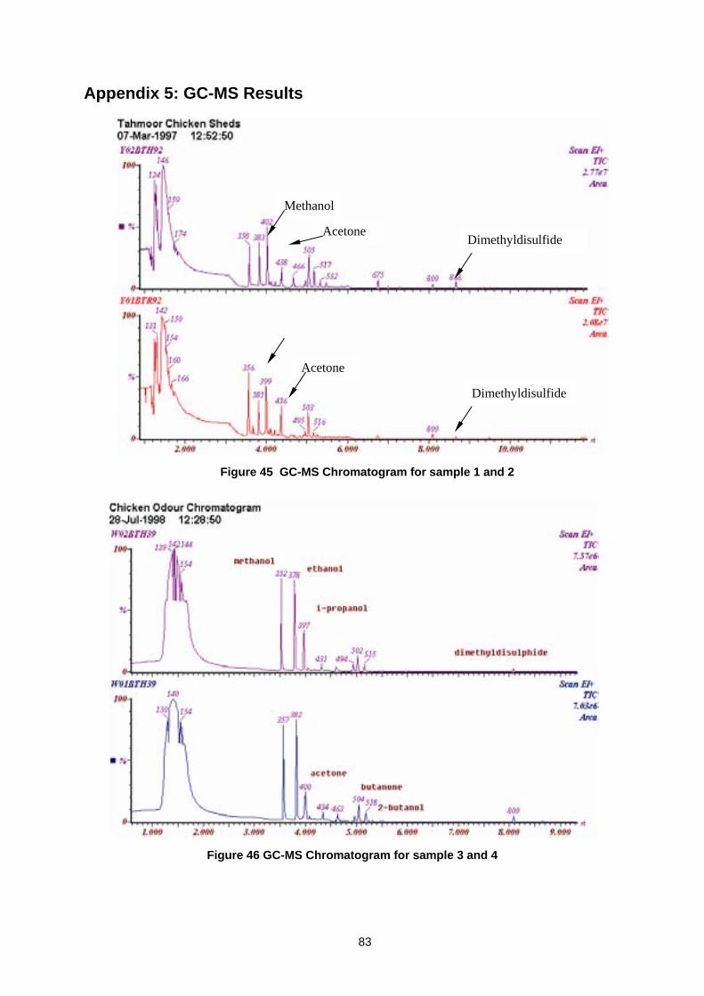
83

Appendix 5: GC-MS Results

Figure 46 GC-MS Chromatogram for sample 3 and 4

Methanol

Figure 45 GC-MS Chromatogram for sample 1 and 2

Dimethyldisulfide

Dimethyldisulfide

Acetone

Methanol

Acetone

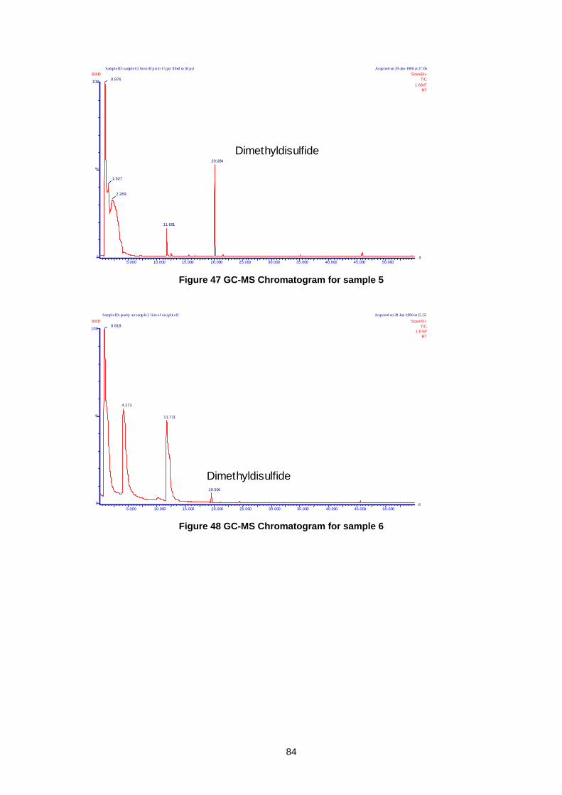
84

Acquired on 29-Jun-1998 at 17:06Sample ID: sample #2 from 30 psi to 15 psi filled to 30 psi

5.000 10.000 15.000 20.000 25.000 30.000 35.000 40.000 45.000 50.000rt 0

100

%

0.876

20.084 1.527

2.269

11.691

Scan EI+ TIC

1.66e7 RT

B840

Dimethyldisulfide

Figure 47 GC-MS Chromatogram for sample 5

Acquired on 28-Jun-1998 at 15:52:Sample ID: poulty air sample 2 litre of air split off

5.000 10.000 15.000 20.000 25.000 30.000 35.000 40.000 45.000 50.000rt 0

100

%

0.818

4.171 11.711

19.504

Scan EI+ TIC

1.67e7 RT

B837

Dimethyldisulfide

Figure 48 GC-MS Chromatogram for sample 6

85

Acquired on 02-Aug-1998 at 19:47:Sample ID: can 1175 b

15.000 17.500 20.000 22.500 25.000 27.500 30.000 32.500 35.000 37.500 40.000 42.500 45.000 47.500 50.000 rt 0

100

%

23.761

22.393

16.512

19.565 17.029

20.057

24.862 49.537 48.686

38.742 33.921 27.022 28.315 40.486

46.876 44.732

Scan EI+ TIC

1.41e7 RT

B864

Dimethyl Disulphide

Figure 49 GC-MS Chromatogram for sample 7 Acquired on 03-Aug-1998 at 12:07:Sample ID: can 1176

15.000 17.500 20.000 22.500 25.000 27.500 30.000 32.500 35.000 37.500 40.000 42.500 45.000 47.500 50.000 rt 0

100

%

23.671

22.536 16.503

19.508

24.772 28.342

26.933 33.814

33.406 42.129 44.632

Scan EI+ TIC

1.05e7 RT

B866

Dimethyl Disulphide

Figure 50 GC-MS Chromatogram for sample 8

86

Appendix 6: Odour community survey letter and forms 11 January 1997

To the household

Dear Sir/Madam,

Odour community survey in relation to a study on odour emission reduction from chicken broiler growout farms

The University of New South Wales is undertaking a study on odour and ammonia emissions from broiler chicken farms. The study is funded by the Rural Industries Research and Development Corporation and is being carried out in conjunction with the NSW Chicken Growers Association over a two years time frame. The aim of the community survey is to find out how the residents of your area experience odours present in the environment.

The purpose of this letter is to seek your assistance in completing survey forms over a 10 week period to help us measure the effect of odours from broiler chicken farms on other nearby properties.

Why is a survey being carried out?

The aim of the odour community survey is not just to determine air quality at an isolated moment in time, but also to record how people perceive odours present in the air over a longer period. The information obtained should, for instance, contribute to an investigation of the effects of weather and seasonal variations on the odour in outside air.

Comments and information provided throughout the survey process will be related to factors such as chicken age, weather conditions, environmental conditions within the broiler chicken sheds and other relevant factors. The results of the survey will help to understand odour transportation processes associated with poultry odour emissions and to relate the processes to odour levels experienced on nearby properties.

Where is the study taking place?

The first phase of the study in NSW will be carried out in relation to two farms including the [Name of farm]. We are asking residents within a one kilometer radius of the farm to record their assessment of the odour in the outside air near their home over a 10 week period including one entire chicken growing batch. The data recorded should provide a reliable basis to establish the extent of odour dispersion and its overall effect.

When is the study taking place?

The initial community study will commence on the 16th January 1997 and go on for a period of 10 weeks. A further less intensive study involving fewer residents will be undertaken over the following 10 months.

87

How is the study to be conducted?

During the study period residents are asked to undertake a daily assessment of the quality of the outdoor air. Each assessment will take only about three minutes. The assessment involves residents going outside their house and breathing and assessing the outside air between 6:00 pm and 8:00 pm. Forms for recording results will be provided to residents and collected once or twice a week.

Even if you are not affected by odour it is requested that you please still complete survey forms as the more information that is collected the more reliable will be the outcome of the survey. As we are trying to determine how far poultry odours will travel, it is important that we receive information on zero effects.

During the survey, we will encourage you to record your own impression of the odours you smell. This is a particularly important aspect of the survey.

As the survey will be of great importance for improving environmental air quality in the area, we urge you to participate in the study. If you are willing to give your services for this study for the entire period, you are requested to kindly fill in the enclosed form which will be collected by one of our project team members. Any resident aged 18 or over who is willing to take part can fill out a form and participate in the study. Your reply and your personal data will be treated in strict confidence.

I hope that many volunteers are willing to give their help in this survey.

Yours faithfully,

John Jiang

88

Resident details

Resident surname:

First name:

Age:

Sex:

Address:

Telephone (H)

Telephone (alternative)

How many people in above residence:

What is your profession?

What level of school:

preliminary school high school

technical college university

other (please specify)

How long have you been lived at this address: Months Years

Where do you spend the greatest part of you day? Away from home at home

In your option, do people in general

1. pay far too little attention to the environment?

2. pay too little attention to the environment?

3. pay sufficient attention to the environment

4. pay more than enough attention to the environment

Do you have any comments on the odours you smell?

Declaration of content:

As a participating resident, I agree that the above personal data (name, address, age, sex, etc.) on myself can be collected and stored within the scope of the above odour survey. After completion of the investigation or if I withdraw from the survey, my name and address will be erased. I consent to the use of the remaining data in anonymous form for scientific purposes.

Signature: Date:

89

Odour Survey Form

Resident surname: First name: Address:

Telephone (h) Telephone (alternative)

Where were you when you first smelled the odour?

Inside house

Outside house

Just outside own property

Elsewhere How strong was the odour when you first smelled it? Would you say the odour was:

No odour (0)

Very faint (1)

Faint (2)

Distinct (3)

Strong (4)

Very strong (5) What would you say the odour smells like? The list of descriptors is to help you describe what the odour smells like (Please check all the descriptions)

Rotten eggs (H2S) Ammonia

Fishy Low Tide

Plastic Asphalt

Nail Polish Damp Earth

Weed Killer Garbage

Craft Glue Gasoline

Paint Household Gas

Cat Urine Burnt Rubber

Compost Linseed Oil

Feathers Can’t describe

Other (specify)

Where do you think the odour is coming from?

Any other comments relating to odours during past 24 hours:

Signature: Date:

90

Appendix 7: Odour concentration during the transportation Four duplicates of odour samples have been tested on the affects of air transportation on odour concentration level. Each duplicate was sampled in sequence. In the first two duplicates of odour samples (Week 6), the odour concentration was very low and therefore, third and fourth duplicates of samples (Week 7) were arranged again.

In the first test, two duplicates of odour samples (collected at 12:00 am and 4:00 pm, respectively) were sent to Melbourne from the Sydney airport at 5:00 pm. The package was sent back the next available freight (7:40 pm) and picked up in the next morning at about 9:00 am. The panel started at 10:00 am and finished at 1:00 pm. The samples were tested with 24 hours.

In the second test, two duplicates of odour samples were collected at 10:40 am and 2:40 pm, respectively. Unfortunately, the Melbourne airport did not send the package back to Sydney until the next day at 10:00 am. These samples were not picked up until 12:00 am in the next day. The samples were tested within 32 hours.

Figure 51 and Figure 52 show the air temperature during the sample transportation for the first and second test, respectively.

Figure 53 shows the odour concentration levels for each duplicate. If an analytical error of 40% for olfactometry is taken into account, the results (even for second test) have shown that the odour concentrations were not affected by the air transportation.

0

5

10

15

20

25

30

0:00 2:00 4:00 6:00 8:00 10:00 12:00 14:00 16:00 18:00 20:00 22:00 0:00 2:00 4:00 6:00 8:00

Aircarft departed from Sydney

Aircarft arrived at Melbourne

Aircarft departed from Melbourne

Aircarft arrived at Sydney

Sample picked up

Figure 51 Air temperature on 5 August 1999

91

0

5

10

15

20

25

30

35

40

0:00 3:00 6:00 9:00 12:00 15:00 18:00 21:00 0:00 3:00 6:00 9:00 12:00 15:00 18:00 21:00

Hours of the day, hr

Aircarft arrived at Melbourne

Aircarft departed from Melbourne

Aircarft arrived at Sydney

Aircarft departed from Sydney

Sample picked up

Temperature

Figure 52 Air temperature on 12 August 1999

0

100

200

300

400

500

600

700

1 2 3 4

Sample Numbers

Odo

ur c

onc.

, OU

/m3

Without airfreightWith airfreight

Figure 53 Odour concentrations for duplicate samples

92

Appendix 8: Photographs

Figure 54 Modern tunnel ventilated shed

Figure 55 Inside a tunnel ventilated shed

93

Figure 56 Sampling drum

94

Figure 57 Data logger system

Figure 58 Olfactometry testing

95

96