Unmixing of Spectral Components Affecting AVIRIS Imagery of Tampa Bay

Kendall 1. Carder, ?.P. Lee, Robert F. Chen

University of South FloridaDepartment of Marine Science

140 Seventh Avenue SouthSt, Petersburg, FL 3370]-50]6

Curtiss 0, Davis

Jet Propulsion LaboratoryCalifornia Institute of Oceanography

4800 Oak Grove Blvd.Pasadena, CA 91109

According to Kirk’s as well as Morel and Gentili ’s Monte Carlo simulations, thepopular simple expression, R~O.33b~a, relating subsurface irradiance reflectance (R)to the ratio of the backscattering coefficient (bb) to absorption coefficient (a), isnot valid for b/a > 0.25. This means that it may no longer be valid for values ofremc)te-sensing reflectance (above-surface ratio of water-leaving radiance todownwelling irradiance) where R,, > 0.0]. Since there has been no simple R, expressiondeveloped for very turbid waters, we developed one based in part on ~onte Carlosimulations and empirical adjustments to an Rpq model and applied it to rather turbidcoastal waters near Iampa Bay to evaluate Its utility for unmixing the opticalcomponents affecting the water-leaving radiance. With the high spectral (lOnm) andspatial (20n12) resolution of Airborne Visible-InfraRed Imaging Spectrometer (AVIRIS)data, the water depth and bottom type were deduced using the model for shallow waters.Bottom types included sand, grass flats, and emergent vegetation, with a variety oflevels of wave and current-induced suspended sediments apparent in the imagery. It alsoincluded turbid water in a deep ship channel that had been scoured off an adjacentshoal region, creating the appearance of a “false” bottom at about 1.5m. This researchdemonstrates the necessity of further research to improve interpretations of sceneswith highly variable turbid waters, and it emphasizes the utility of high spectral-resolution data as from AVIRIS for better understanding complicated coastalenvironments such as the west Florida shelf.

J.___dNIRODUCIION

Models have been developed for use with hyperspectral remote-sensing ~~flectaricedata collected just above the air-sea interface for the West Florida Shelf , ,3s4. lheyrespond to variations in pigment, detrital, and gel bstoff absorption, chlorophyll a andgelbstoff fluorescence, water Raman scattering, backscattering by water andparticulate, and bottom depth and albedo. To date these models have not beensystematically used to interpret hyperspectral data derived from high altitude airbc~rnesensors, which can provide a wide variation in component contributions in a singlescene.

AVIRIS (Airborne Visible-InfraRed Imaging Spectrometer) is a test bed for futurespacecraft imaging spectrometers that may be in orbit in the next century. AVIRIS was

I

designed largely for terrestrial applications requiring high spectral (lOnm) andspatial (20m2) resolutions. It has 224 spectral channels from400 to 2400nm, 20m squarepixels when viewing the Earth from 65,000 feet altitude, and it had about 10-20% of thesignal-to-noise (S/N) of the Coastal Zone Color Scanner (C7CS) in 1990, when the datareported were acquired. For coastal ocean applications much larger signals are typicalcompared to those offshore. Thus, adequate signal levels for manY nearsh[]reapplications can be achieved by binning 25 to 100 pixels togethers.

In March 1990, AVIRIS data were collected from a NASA ER-2 aircraft flying at65,000 feet altitude on two SW-NE flight lines across the West Florida Shelf and intothe mouth of lampa Bay. lhese lines were flown at about 1515 Eastern Standard lime anda total of 16 scenes were collected.

The AVIRISprefl ightcalibrati on was adjusted to be consistent with the in-flightperformance of the instruments. lhe recalibrated data, representing total radiance atthe sensor, was then partitioned into atmospheric path radiance and radiance upwelledfrom beneath the water surfaces (water-leaving radiance).

lhe water-leaving radiance values collected on a windy day near the mouth oflampa Bay by AVIRIS were very bright, with the maximum remote-sensing reflectance R,.values (thelratio of the water-leaving radiance to the downwelling irradiance) of about0.035 Ster (symbols used in this text are listed in Table 1), even for the deep shipchannels. In eneral, maximum 11~~-? value for open ocean stations range from about 0,005to 0.01 ster . The high R,, values for the Bay at the time of the study suggest thatthe bottom depth was very shallow or the water was very turbid due to the high windsand tidal currents. Ibis enigma can be better ‘understood by modeling the R,, spectra.

2..MODEL DEVELOPMENT

Remote sensing reflectance R,. is defined as the ratio of the above surfacewater-leaving radiance LW(O+) to downwelling irradiance Ed(O+), so

LW(O+)R,*=—---Ed(o+) (1)

andR*,’o.533~-

Q(2)

where R=EU(O-)/Ed(O-) is the subsurface irradiance reflectance, 0.533 coyes from theair-sea interface effectb, and Q=E,(O-)/LU(O-) is the so called “Q factor “, which isreported in the range of 3 to 121’s.

For homogeneous, deep water, Kirk9 as well as Morel and Gentili10 simplified Rby using Monte Carlo simulations, where bb is the total backsc:ttering coefficient (asum of backscattering coefficients from molecules b

b and ‘articulates b%) ‘w;tl; a.,the total absorption coefficient (a sum of absorption coefficients o

R=f.:- (3)

I

particulate a and gel bstoff a ). The parameter f = 0,33 forb~a < 0.;511 but f is non-constant for ~~a > 0.25 suc~ thatlof decreases as b a increases I

(and it also

increases with increasing sun angle . When b~a > 0.2 , R,$ will be > 0,0 stern’assuming3’12’13 a general Q - 3.5. Thus, when R -1is far greater than 0.01 ster , f wil~vary with bt/a instead of remaining a spectrar~ constant for a given sun angle.

AVIRIS-derived R,$ values of Tampa Bay were of order 0,03 ster”l and f wasadjusted in a manner consistent with data in Kirk’s Fig. 59:

f’oo33(l-e.~) (4)

where c is a small constant. Data from Kirk’s9 and Morel and Gentili ’s10 Monte Carlosimulations suggest values of e ranging from 0.2 to 0.4. We found a value of c*O.33worked well for our situation. lhen R.. is exDress@d as

IS r ‘- ‘ – ‘-

// ~176(1c4)4rs “

!--

a aQ(5)

which results upon combination of Eqs. 2-4.

Lee et al.3’L proposed that b~Q can be expressed in the form

(6)

where the final term is an expression for b#QP. The subscripts “m” and “p” designatemolecular and particulate components, respectively.

Thus,

(7)

pro~il~e~ an estimate of bb for use in Eq. ‘#’. If Q is assumed to be equal to about3.5’ ‘ , then R,= for homogeneous, deep, turbid water is

0.176 [1--1-J-]6~-- (-+rn+x(Efw*, . b,>- .RZB--- ---–- --- --–---–—.--~:’ ..-——. ..—-——

a ‘z+x(? “ ‘(8)

where values for bh are readily available14, and Qm values vary with sun angle3’4. Forthis study, the sun angle was about 49°, so Qm~3.9 is used3’4.

Due to the shallow water depth in coastal waters, the water-leaving radiance 1can in general be expressed as a sum of two components: LCOI from the scattering an(!attenuation of molecules and particles in the water column, and Lb is the radiancefrom the bottom reflection. Since coastal waters can be quite tur~id, water Raman

r

b

scattering and fluorescence \ from colo,red dissolved organic matter (C~OM) are typicallynegligible (see lee et al. ). For this truncated water column, R~~cO is adjusted as

Rry+r:ovl- e-3”2(a+bJH] (9)

where R,~C”p come~ from [q. 8, and the 3,2 in the exponential term is3Dd in lee et al, . The 2.7(a+bb) term in Eq.

$jstimated from10 is similarly estimated .

lhe bottom contribution R,,kt is expressed as

R,yt - 0.l”13pe - 2 . 7 (a+hb)H

where p is the bottom albedo, and H the bottom depth.

For the purpose of modeling and unmixing the spectralthe R,. curves measured by AVIRIS, X,Y,p,}l and a must betotal absorption coefficient a, aw is known from Smith and

ag=ag(440) e-s(~-440) ,

and aP, the particle absorption coefficient is calculatedpigment-specific absorption curve, typical to the reqiori.

(lo)

components contributing toderived. To determine theBaker14, ag is expressed as

(11)

as aP**[C], where a ● ‘Iwo Parameters a.(4$O)1;n~

a ~440) are used to adj”ust the levels-of a and ap in tie model by using measfi~ed ;urve6s apes consistent with those involved in !he study area. Also the bottom depth H andbottom albedo p must be estimated to model R,,bt, This means, at least six parametersare needed to accomplish the unmixing if the spectral dependencies of aP, ao, and p areknown.

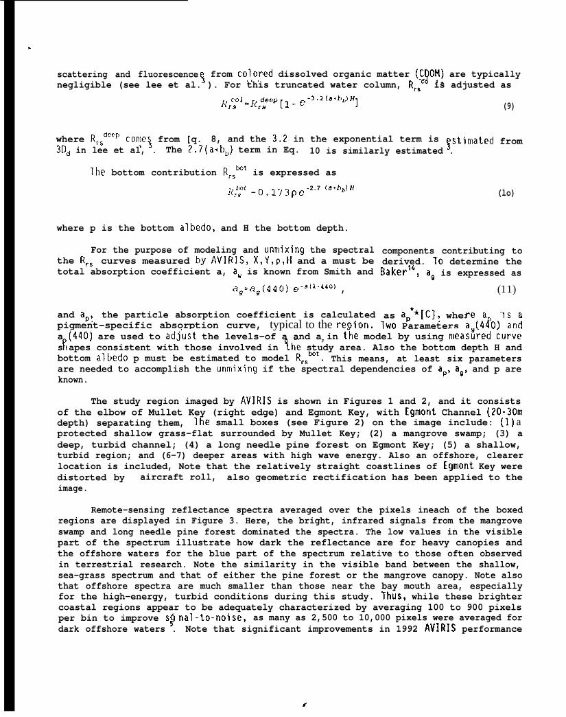
The study region imaged by AVIRIS is shown in Figures 1 and 2, and it consistsof the elbow of Mullet Key (right edge) and Egmont Key, with Egmont Channel (20-30mdepth) separating them, lhe small boxes (see Figure 2) on the image include: (1) aprotected shallow grass-flat surrounded by Mullet Key; (2) a mangrove swamp; (3) adeep, turbid channel; (4) a long needle pine forest on Egmont Key; (5) a shallow,turbid region; and (6-7) deeper areas with high wave energy. Also an offshore, clearerlocation is included, Note that the relatively straight coastlines of Egmont Key weredistorted by aircraft roll, also geometric rectification has been applied to theimage.

Remote-sensing reflectance spectra averaged over the pixels ineach of the boxedregions are displayed in Figure 3. Here, the bright, infrared signals from the mangroveswamp and long needle pine forest dominated the spectra. The low values in the visiblepart of the spectrum illustrate how dark the reflectance are for heavy canopies andthe offshore waters for the blue part of the spectrum relative to those often observedin terrestrial research. Note the similarity in the visible band between the shallow,sea-grass spectrum and that of either the pine forest or the mangrove canopy. Note alsothat offshore spectra are much smaller than those near the bay mouth area, especiallyfor the high-energy, turbid conditions during this study. Thus, while these brightercoastal regions appear to be adequately characterized by averaging 100 to 900 pixelsper bin to improve si nal-to-noise,!$ as many as 2,500 to 10,000 pixels were averaged fordark offshore waters . Note that significant improvements in 1992 AVIRIS performance

f

have reduced the binning requirements for recently acquired (November 1992) coastalscenes to as few as 25 pixels.

Even with pixel-binning, there remain some irregularities “,{n the spectra due toin part to coherent noise in 1990 AVIRIS scenes (Hamilton et al. ) and low signal.to-noise ratios. Recent improvement in AVIRIS performance have also eliminated coherentnoise effects, Because of residual noise in the 1990 no attempt was made to model R,~spectral curves for wavelengths shorter than 420nm or longer than 680nm.

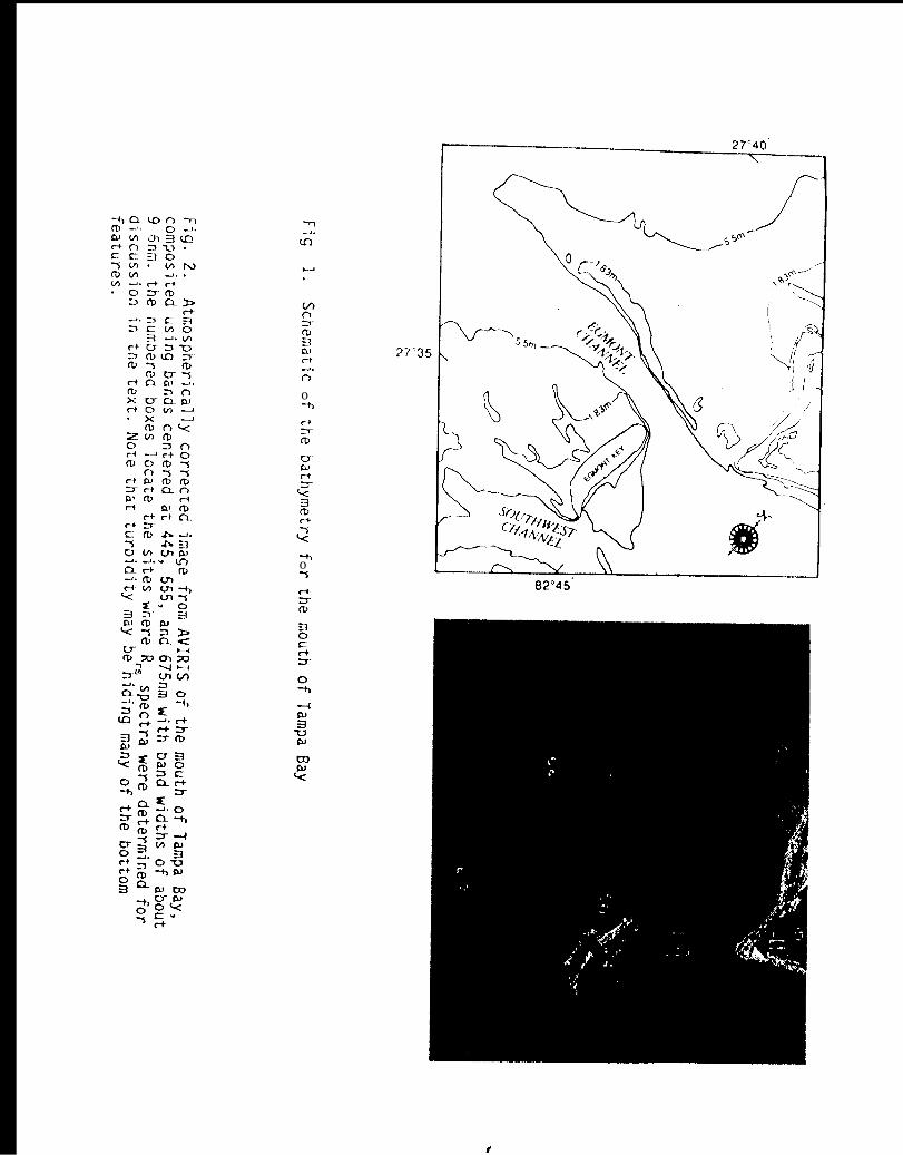
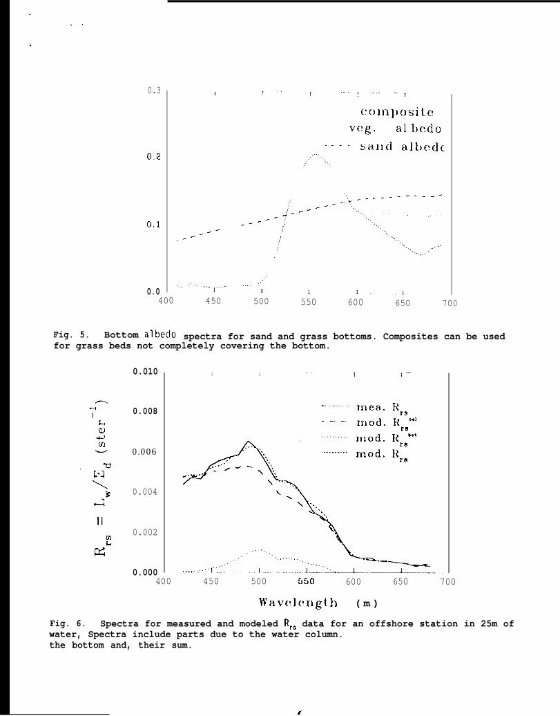
Field data collected by sampling from the R/V Bellowss indicate that the slopes of the spectral semi logarithmic line describing a for the Bay mouth area is about0,013nnf1 (see Eq.11 and Figure 4), and the shapes o? the particle absorption spectracan be represented by the curve in Figure 4. Shapes for the albedo curves used in themodel for sand and grass bottoms are shown in Figure 5.

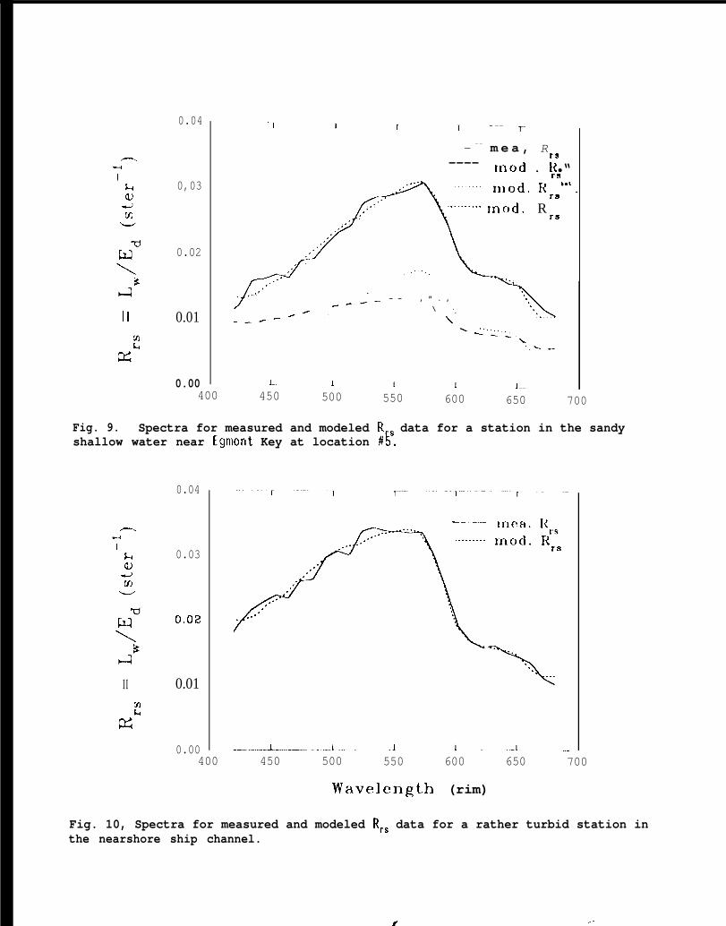
Contributions due to aP, a~, and p were modified by varying aQ(440), aP(440) andp(500) and used in the R,, model for the various study sites. Table 2 and Figures 6-11show the model parameters and results for the selected locations. Rather good agreementbetween the measured and the modeled R,, curves was found with a general discrepancyof less than 5%, lhis difference derives from the combination of errors associated withatmosphere correction, aP and p curves, model parametrization, and noise in the AVIRISdata.

lhe model parameters used for the offshore location Fig,6) are similar to thoseused for modeling offshore RC~ 4curves measured from a ship with a small difference inY likely due to a -2-hour time difference between ship and AVIRIS measurements. Forlocation 1 (Figure 7), which is inside the elbow of Mullet Key, a spectral lycompositedbottom albedo (see Figure 5) was used to simulate bottom albedos containing a mixtureof pixels containing both sea grass and sand bottom within the sample box of an AVIRISimage. The derived bottom depth is close to the depth for that site from the NOMbathymetric chart (fl1414). Also the higher values for aP(440) and ag(440) and thelower values forX and p(500) for this site compared to those from the more energy-richfgmont channel area result from a smaller impact of resuspended sediments on thebackscattering coefficient in the protected area of the elbow of Mullet Key.

For locations 3 and 5 (see Figures 8 and 9), the AVIRIS-derived R,. curves lookvery similar, as do the derived parameters (see Figure 3 and Table 2). But from thechart, location 3 is in the Egmont ship channel, with a bottom depth of --15m, whilelocation 5 is close to Egmont Key with a water depth of--l.5m. An explanation for thisdichotornymay be that wave-induced erosion and currents scoured the sediments off theshoal area north of the channel and transported them over the channel, where they beganto settle. This could have made the optically-averaged water-leaving radiance appearto be from a shallow water column of -1.4m. Without ship data to confirm thisspeculation, model values for location 5 will be only used to illustrate theuncertainties involved for optically structured water column.

The Tampa Bay mouth region (location 3,5,6, and 7) has about 2-8 times greateraP(440) and a (440), and 10-70 times higher X values than the offshore area. Since X1s largely a#ected by changes in scattering, it suggests that the brighter image ofthe mouth area is due to large concentrations of suspended particles, and is not

.

b

entirely due to the effects of radiance reflected from the bottom .

The derived H for this region was within 20% of the NOAA Chart depth, and most~in 10% of the chart depth. The differences may have resulted frommodel depths were WI

errors in the atmospheric correction, uncertainty in the aw (the accuracy of aW isabout ~lO%’L), or perhaps due to vertical inhomogeneity in the suspended particles inthe water column.

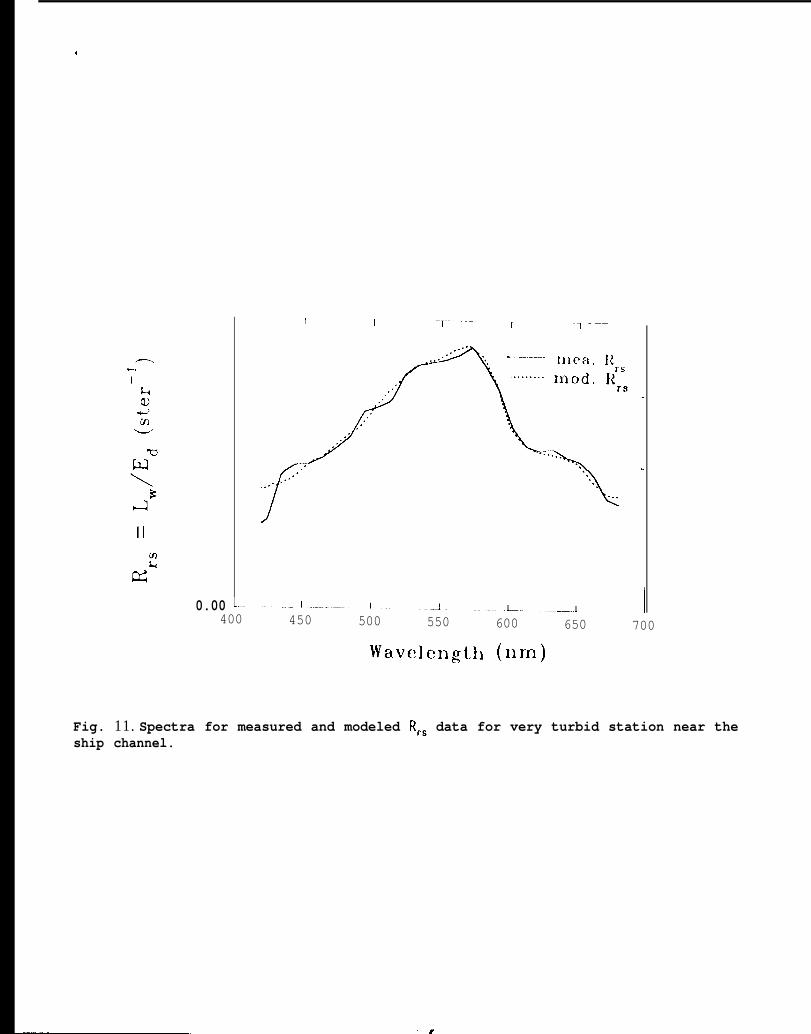
[or the optically deep locations (except location 3), we found that the proposedR,, expression worked well for the turbid waters of this region, Further study,however, with corroborating ship-derived data is needed to better confirm thisobservation,

4, SUMMARY

1. Careful removal of atmospheric effects and vicarious recalibration of AVIRISyields spectral R,, curves which can be modeled using mixtures of optical contributionsfrom various components: water molecules, CDOM, suspended particles, and the seabottom,

2. For the turbid regions for which R model curves were derived, thereflectance was nonlinear with b~a, e.g. R=O.33{!-eb~a)b~a, and an Q, value of 0.33worked well for the model in our study area.

3. Close agreement between curves for AVIRIS-derived R,~ and modeled Rp was foundfor a complex, coastal environment, with most derived water column depth va?ues foundto be within about 10% of charted depths for the shallow locations.

4. lhe high X values found at the mouth oflampa Bay suggest that backscatteringfrom suspended particles contributed significantly to the remote-sensing reflectancevalues determined there.

5. lhedeep location in Egmont channel (location 3) provided an Rr~curve similarto that expected for shallow water (e.g. see location 5). One explanation for this maybe that a “false bottom” reflectance from suspended sediments scoured from the adjacentshoal region to the north formed at about 1.5m below the surface. The model dependsupon an assumption of vertical homogeneity in water-column properties, which was likelyviolated for this location.

6, As one might expect, R,~ curves for shallow sea grass beds were nearlyidentical to those for emergent vegetation for wavelengths shorter than about 580nm.

Special thanks to Robert Steward, Thomas Peacock, David Costello, and Lisa Young fortheir help in laboratory analyses. Financial support was provided by the NationalAeronautics and S~ace Administration to the University of South Florida (USF) throughgrant NAGW-465, GSFC contract NAS5-30779,Office of Naval Research through grantprovided by the State of Florida through

and JPL contract 958914 (RE-198), and byNOOO14-89-J-1O91 to USF. Ship supportthe Florida Institute of Oceanography.

thewas

1,

●

Jable 2. R,. mode’

Jable 1. Symbols and units

LJO+)1LCOL

Lfi’tI”)EJo-)Ed(O-)Ed(O’)Rrs

Rabb

!Qs

= surface leaving radiance from water+~r emergent plants, Wm-2ster-1= radiance from water column, Wm”2ster= radiance from bottom reflectance, Wn~-2ster-1= subsurface upwelling radiance, Wm-2ster-’= subsurface upwelling irradiance, Win-2= subsurface downwelling irradiance, Wm”2= above surface downwelling irradiance, Win-2= remote sensing reflectance, ster-l= irradiance reflectance= absorption coefficient, m-l= backscattering coefficient, m“l= bottom albedo= water depth, m= ratio of upwelling irradiance to radiance, ster= spectral slope parameter (rim-l)

parameters used to fit the data for locations shown in Figure 2.

.—.. .._-_ G---- .—--x_—.s_--. ——-. -———..---

Locations aP(440) ag(440) x Y p(soo) H~ HWB—.—...

offshore 0.036 0.037 0.00086 1.8 0.50 25.0 24.7—.....——.-.—. . ..— —. .—. .__. __ _ _ _ —... .— .. ———. —. .——. ——

#l 0.206 0.320 0.008 0 0.08 1.1 0.9.——__- . . .._—. . . .._ . . . . ___________ —

#3 0.152 0.033 0.017 0 0.14 1.4 15——- . ..—-—. ..- . .-— ,.. — .—.. — -—..—— .———. . ..— . . . ___ _ _ _ _

#5 0.195 0.070 0.021 0 0.15 1.3 1.5— — . .. —- —- . ..—. . . . . . . . . . . . . . .—

#6 0.137 0.100 0,035 0 10—-------- ..— — —. ———. —-.. —.. .—— —. —.——-.——

#7 0.290 0.170 0.055 0 3.3.——. ——. - ..-. .—. —-... ——-=— __... ,. .-. -___— J——. -——.. .. ——-=-.-.:=:—.-.-—..—— —.—

Note: H@, comes from Chart il1414means i{ can be seen as optically

of NOAA. Where the location has no p(500) and tl~deep water.

6 de f.e.cg.n~e.s1. Carder, K.L. and R.G. Steward, 1985, “A remote sensing reflectance model of a red

tide dinoflagellate off West Florida,” [imnol. Oceanogr. 30(2), 286-298.2. Carder, K.L., R.G. Steward, J,H. Paul andG.A. Vargo, 1986, “Relationshipsb etween

chlorophyll and ocean color constituents as they affect remote sensing reflectancemodels, ” [imnol. Oceanogr. 31(2), 403-413.3, Lee, Z.P,, K.1. Carder, S.K. Hawes, R.G, Steward, I.G. Peacock and C.O. Davis,

1992, “An interpretation of high spectral resolution remote sensing reflectance”,Optics of the Air-Sea Interface, Proc, SPIE, Vol. 1749, 49-64,

4, Lee, Z,P,, K.L. Carder, S,K. Hawes, R.G. Steward, I.G. Peacock and C.O. Davis,1993, “A Model for Interpretation of tiyperspectral Remote Sensing Reflectance”, Appl.Optics, submitted.

5. Carder, K.L., P. Reinersman, R.G. Steward, R.F. Chen, F. Muller-Karger, C.O.Davis, and M. Hamilton, 1993, “AVIRIS Calibration and Application in Coastal OceanicEnvironments,” Remote Sensing of the environment, Special Issueon Imaging Spectrometry(G. Vane, editor), in press.6. Austin, R.W., 1974, “Inherent spectral radiance signatures of the ocean surface,”

Ocean Co70r Analysis, S10 Ref. 7410, ADril.7. Austin, R.W,, i979, “Coastal ~one color scanner radiometry”, Ocean Optics VI,

Proc. SPIE. 208. 170-177,8. Gordon, Ii.’R., R.C. Smith, and J.R,V. Zaneveld, 1979, “Introduction to Ocean

Optics, ” Ocean Optics V], Proc. SPIE. 208, 15-63.9. Kirk, J.T.O., )991, “Volume scattering function, average cosines, and the

underwater light field,” Limnol, Oceanogr. 36(3), 455-467.10. Morel, A. and B. Gentili, 1991, “Diffuse reflectance of oceanic waters: its

dependence on sun angle as influenced by the molecular scattering contribution”, Appl.Optics 30, 4427-4438.

11. Jerome, J.H., R.P, Bukata and J.E. Bruton, 1988, “Utilizing the components ofvector irradiance to estimate the scalar irradiance in natural waters,” Appl. Optics27(19), 4012-4018.

12. Gordon, H,R., O.B. Brown and M,M. Jacobs, 1975, “Computed relationship betweenthe inherent and apparent optical properties of a flat homogeneous ocean,” Appl. Optics14,’ 417-427.

13. Gordon, H.R., O,B. Brown, R.H. Evans, J.W. Brown, R.C. Smith, K.S. Baker, andD.K. Clark, 1988,” A Semianalytic Radiance Model of Ocean Color”, J. Geophys. /?es.93(D9), 10,909-10,924.

14. Smith, R. C. and K.S. Baker, 1981, “Optical properties ofwaters,” App?. Optics 20(2), 177-184.

15. Hamilton, M., C.O. Davis, S.H. Pilorz, W.J. Rhea, and“Examin ationofChlorophyll Distribution in Lake Tahoe, Using theInfrared Imaging Spectrometer (AVIRIS), Proceedings of the ThirdPub. , No. 91-28.

the clearest natural

K.L. Carder, 1991,Airborne Visible andNIR2S//orkshop, JPL

i .=,.-,

--1.

f-l

o-+)

-ho-f.-+

t

0.10

mw 0.06

w

0.00400 500 600 700 800

Fig. 3. R,. spectral curves for sites shown on Figure 2. Note that locations 2 and4 contain emergent mangroves and pines, respectively, and location 1 contains a seagrass bed, protected from waves by Mullet Key.

0.5

0.4

0.3

0,2

0.1

0.0---- ..,..,,------ - -. .-..,.

400 450 500 550 600 650 700

waveleI@kl (1-1113)

Fig. 4. Absorption spectral shapes for pure water, particles, and gelbstoff orCDOM .

..,

0.3

0,2

0.1

0.0

I

400

Fig. 5. Bottom albedo

---.>-

. . . . . . . . . . . . . . ,,. ~......

450

Com])ositeVcg. al bc!clc)

,,.,,. . . . . . . .I 1 1 . .— 1

500 550 600 650 700

spectra for sand and grass bottoms. Composites can be usedfor grass beds not completely covering the bottom.

0.010

0.008

0.006

0.004

0.002

0.000400

I 1 , . .T–- , ..-

450 500 550 600 650 700

Wavc!lc?Ilgth ( m )

Fig. 6. Spectra for measured and modeled R,. data for an offshore station in 25m ofwater, Spectra include parts due to the water column.the bottom and, their sum.

#

---.-4

I&a.)

+-Ju-lw

II

0.03

0,02

0,01

r 1 I T “-” r

-—.Inc!a . R rs- - -II-I Od . R ““’

rs

III C)CI. R ‘“’ _rs

““”””” xnod, 1<rs

f. . . . . ,,. ---=----- --.--. ,---- - --- —___ -

. . . . . - -

0,00 L I 1 . 1 1 . . 1.- 1400 450 500 550 600 650 700

Fig. 7, Spectra for measured and modeled R,, data for a station over a grass bed atlocation il.

0,04

II 0.01

0.00

-.I ‘1 I T “ , .

‘------- In e a. 1{

r3-—_ mod. R ‘*’

rs

~~~~~~~~ Inod. N b“’,----

[~

rs

..’” +“--”-””- mod. R,, rs..-

. . .

./’’’””

,,, ..,,

. . .. . . ..- .,”

\

. . .

“.,...,- -. — — - -. \ ., “.

_- -,-,, \ , ‘.

- — - . . . . .,,.\ “’....,..,,,,. ,,

,,, =-_-’.,..’

,. ..., <._.,, .

l-_ 1 1 ----- .1 ._ I_. __.. __

400 450 500 ’550 600 650 700

Wavclen~t}~ (1~111)

Fig, 8. Spectra for measured and modeled R,. data for a station over the shipchannel at location i3.

-.’-4

I&a)

+-J

V)w

II

0.04

0,03

0.02

0.01

0.00400

“1 T 1 T ‘-- ~.

R- -- m e a , ~~---- mod . }< ● “

rs.. ”-’ n]od. Ii ‘“’.

/“\

., rs. . .

““””-”””” Inod. R,’ rs. . .

,,

,“. .

.,

.J

.,

[

-.,.””

\

. . .

. ..’ ,, ‘.- - , ” . ,

/~--- ‘.\ ‘. ‘.

_==. ,. . . . . .-e-

\“ . ...,.,,--<,

\.,. _

l-. J I 1 l__

450 500 550 600 650 700

Fig. 9. Spectra for measured and modeled R, data for a station in the sandyshallow water near Egmont Key at location #~.

0.04

I& 0.03a)

-@mw

II 0.01

0.00400 450 500 550 600 650 700

Wavelength (rim)

Fig. 10, Spectra for measured and modeled R,, data for a rather turbid station inthe nearshore ship channel.

f ,-

--4

IL

II

0.00 L-400

r I -T_. -----“”1 ... ___ _

I450 500 550 600 650 700

Wavelen@}l (Ill-n)

Fig. 11. Spectra for measured and modeled R,~ data for very turbid station near theship channel.