University of WurzburgInstitute of Computer Science

Research Report Series

Performance Evaluation of Interference andCell Loading in UMTS Networks

Kenji Leibnitz and Armin Krauß

Report No. 268 February 2001

University of WurzburgDepartment of Distributed Systems (Informatik III)

Am Hubland, D-97074 Wurzburg, GermanyTel: (+49) 931 888 6653, Fax: (+49) 931 888 6632

fleibnitz,kraussg@informatik.uni-wuerzburg.de

Performance Evaluation of Interference and Cell Loading in UMTSNetworks

Kenji Leibnitz and Armin KraußUniversity of Wurzburg

Department of Distributed Systems (Informatik III)Am Hubland, D-97074 Wurzburg, Germany

Tel: (+49) 931 888 6653, Fax: (+49) 931 888 6632fleibnitz,kraussg@informatik.uni-wuerzburg.de

Abstract

Third generation (3G) wireless systems will be operating with Wideband Code Di-vision Multiple Access (WCDMA) over the air interface. This access technologyrequires a tight power control by the base station on the uplink in order to reducethe interference in the cell and thus increase the capacity. Furthermore, with theintroduction of 3G systems, data services will be offered that permit data rates ofup to 2 Mbps and varying quality of service requirements in terms of received bit-energy-to-noise ratio. In this paper we will present a performance evaluation of aWCDMA system that is based on a simulation of the power control loops on theuplink in order to investigate the influence of the traffic given by the user distribu-tion and traffic mix on the interference in a cell. Furthermore, we will show that itis possible to use approximations of the power control loops in order to evaluatemore complex scenarios.

1 INTRODUCTION

Wideband Code Division Multiple Access (WCDMA) technology will be the most pro-

minent access technology over the air interface for the upcoming third generation wire-

less systems (3G) [1]. Contrary to second generation networks which are rather lim-

ited to voice services, 3G systems like the Universal Mobile Telecommunication System

(UMTS) in Europe are dedicated to offer data services with high bit rates and flexible

capabilities. Another difference is that the cell capacity is no longer a fixed term, but

also depends on the spatial distribution of the users and their individual services [2].

Thus, the capacity of a UMTS system is limited by the interference caused by each user,

his maximum transmit power, and the type of service given by the data rate and the

activity factor.

This interference limitation leads to the necessity of reducing the transmission power

of each user to a minimum. Mobile stations (MS) will be located at varying distances

1

from the base station (BS, or NodeB). However, if a mobile near the NodeB transmits

with a power level that is too high, it causes too much interference for other MS far-

ther away (“near-far” problem). Additionally, due to shadowing and multi-path fad-

ing there will be variations in the signal strength received at the NodeB. All of this

is overcome by a tight power control performed on the uplink (mobile–to–base station

path). With this power control algorithm the NodeB tries to perform a balancing of the

received bit-energy-to-noise ratios (Eb=N0) of all users in the cell. For these reasons, an

evaluation of the capacity depends heavily on the performance of the power control

loops.

Closed loop power control based on local SIR estimates has been studied by many

authors. While some of the studies contain analytical approaches, e.g. [3, 4, 5, 6], many

researchers have used simulations to investigate the effects of the system parameters

on the efficiency of power control, see [7]. Most of these previously mentioned studies

focus on IS-95 systems operating with a single class of users, however, the complexity

of the model increases rapidly when considering several different classes of users. This

often leads to the case where an analytical performance evaluation reaches its limits

and evaluation by simulation is required [8, 9].

In this paper we will describe a simulation model of the uplink closed loop power

control in UMTS. This model will permit an evaluation of the influence of the user

distribution and the traffic mix on the interference in a cell. The user distribution will

be modeled with a homogeneous spatial Poisson process and we will derive empirical

distributions of the interference caused by the users in the same cell and users from

neighboring cells. Based on the total interference, we will show how the traffic density

impacts the cell loading factor.

This paper is organized as follows. In Section 2 we will give a description of the

detailed closed loop power control model and describe an approximation model that

reduces the computation time. We will show the relationship between the user density,

traffic mix, and the interference in Section 3 and demonstrate that the cell loading factor

is a useful indicator for cell capacity. Numerical results will also be given that indicate

2

the applicability of the approximation method which permits an evaluation of complex

real world scenarios in Section 4.

2 MODELING OF UMTS POWER CONTROL

Figure 1: WCDMA uplink closed loop power control

The closed loop power control on the uplink consists of two interoperating loops

[10, 11], see Fig. 1. Within the inner loop, the BTS continuously monitors the quality of

the uplink in terms of the received Eb=N0 level and compares it with the outer loop

target. If the received value is too high, the MS causes too much interference to its

environment and it is told to decrease its power by a fixed step size. On the other

hand, if the received Eb=N0 is too low, the link quality is not sufficient and a “power-

up” command is sent to the mobile. Such an inner loop correction is performed for

each power control group, 15 times per frame, resulting in a rate of 1500 updates per

second. It should also be noted that an MS in soft handover will be communicating

with the radio network controller (RNC) via all base stations in its active set. In this case

it will also receive several power control commands on the downlink. The MS will

combine the received power control commands and will only increase its power if all

base stations in the active set will demand an increase in transmit power. In our case,

we will consider an inner loop correction step size of 0.5 dB.

After the transmission of a frame is complete, power control enters the outer loop

[12]. A CRC check is performed for each frame at the RNC and the outer loop target

3

value is updated based on the current frame error rate (FER). While the actual outer

loop uses the received FER for updating its target value, we will consider a simplified

case in which we evaluate the bit error rate instead. The reason for this approximation

is that the relationship between Eb=N0 and FER is not straightforward, as it requires an

inclusion of the error rates at modulation, interleaving, and channel coding. Therefore,

we will map the relationship betweenEb=N0 and BER based on the modulation scheme.

Fig. 2 presents the mean Eb=N0 target results from simulations based on different BER

limits.

-2.0

0.0

2.0

4.0

6.0

8.0

10.0

12.0

14.0

16.0

0.0001 0.0010 0.0100 0.1000 1.0000 10.0000

BER limit [%]

Eb/N

ota

rget[d

B]

Figure 2: Measurement of Eb=N0 target

in proportion to BER limit

0.00%

2.00%

0 1 2 3 4 5 6 7 8 9 10 11 12

Frame �

bit

err

or

rate

[%] BER limit

9.0

8.0

7.0

6.0

5.0

4.0

5.0

4.0

5.0

6.0

5.0

0.0

10.0

Eb

/No

targ

et

[dB

]

Eb/No target isincreased

Figure 3: Correlation between the BER

and Eb=N0 target

For a better understanding of the effects of the bit error rate on the resulting E b=N0

target an example is given in Fig. 3. The development of both BER and Eb=N0 target is

presented over a period of 11 frames. The bit error rate exhibits a typical course with

variations from frame to frame. At the end of each frame the outer loop control adjusts

the Eb=N0 target depending on the current bit error rate. This means that if the BER

exceeds the defined BER limit, the Eb=N0 target has to be increased. Otherwise, this

variable will be reduced. So the course of the Eb=N0 target has to be seen with regard

4

to the bit error rate of each frame.

2.1 Approximation Methods for Uplink Power Control

The major computational part of the simulation algorithm (cf. Fig. 1) consists of the

inner loop computation. Furthermore, the purpose of the simulation of power control

groups lies in the adjustment of the mobile stations’ transmit powers. Since the calcu-

lation time required for the simulation of a scenario often turns out as a limiting factor

during detailed examinations, an inner loop algorithm is presented in this section that

includes both, an approximation of the actual transmit power and a significant simpli-

fication of the extensive inner loop mechanism.

The basic idea behind this approximation algorithm is an estimation of the mean

transmit power applied by the power control groups of an inner loop cycle. Since the

inner loop mechanism adjusts the transmit power so that the current Eb=N0 adapts to

the Eb=N0 target, a reverse calculation scheme is used as basis of the approximation

(cf. Fig. 4).

MS NodeB

adjust transmit

power to the

lowest default

value

downlink

channel

uplink

channel

Estimate SIR

Compare SIR

with target

Estimate MS

interferenceone cycle

only

Compute MS

Tx power

Figure 4: Approximated uplink power control loop

The mobile station’s required received power at the NodeB in order to achieve his

Eb=N0 target depends on the total interference affecting the cell. This is the sum of all

received powers including the considered mobile station and can be approximated by

5

12.2 kbps 144 kbps 384 kbpsEb=N0 target 6 dB 3 dB 3 dB

mix1 100% — —mix2 — 100% —mix3 — — 100%mix4 75% 20% 5%

Table 1: Traffic mixes and Eb=N0 targets

taking the value from the previous iteration step. Following this, the received power

can be computed and with consideration of the path loss this leads to the transmit

power. Because the complete inner loop cycle containing the simulation of the power

control groups is now reduced to a single calculation step the required simulation time

is reduced by the factor of 15 (corresponding to the 15 power control groups per frame

in UMTS). This opens the way to simulating more detailed and complex scenarios as

we will show in Section 4.

3 DERIVATION OF CELL LOADING AND NUMERICAL RESULTS

In this section we will give a description of the underlying simulation scenarios and

the user and traffic distributions. For different reference scenarios, we will show the

impacts of the user density on the distribution of the interference received at a certain

cell site. The interference for different traffic distributions leads to a derivation of the

cell loading, which reduces the parameterization of traffic to a single value.

3.1 Scenario Description

Let us consider in the following a regular base station layout as depicted in Figure 5.

Cell sizes are illustrated here with their pilot signal ranges, a parameter which we kept

constant throughout the simulation. Within the considered area, users were randomly

generated following a spatial homogenous Poisson process. In order to consider indi-

vidual data rates, we selected the traffic mixes for all cells and the desired Eb=N0 target

level from Table 1, cf. [13]. A fixed distance of 2 km between each base station was

6

Figure 5: Simulated cell layout

chosen. All simulation runs were performed over a duration of 15000 power control

groups corresponding to a simulation time of 10 seconds after a warm-up period of 5

seconds.

3.2 Evaluation of Inter-Cell and Intra-Cell Interference

The first value that we will investigate is the cumulated interference, distinguished in

interference caused by users in the same cell due to the quasi-orthogonality of the codes

(own-cell interference) and the influence from users of the surrounding tiers of cells on

our observed center cell (other-cell interference). Both terms together constitute the term

which we will denote as total interference Itot.

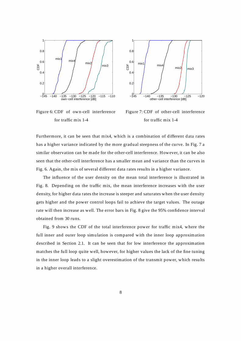
In Fig. 6 the cumulative probability distribution function (CDF) of the own-cell in-

terference is depicted for a fixed scenario with a mean traffic density of 4 users per

km2. Due to the higher spreading gain for 12.2 kbps users in mix1, the least interfer-

ence is created here. The higher the data rates are, the higher is also the interference.

7

−145 −140 −135 −130 −125 −120 −115 −1100

0.2

0.4

0.6

0.8

1

own−cell interference [dB]

CD

F

mix1mix4

mix2mix3

Figure 6: CDF of own-cell interference

for traffic mix 1-4

−145 −140 −135 −130 −125 −1200

0.2

0.4

0.6

0.8

1

other−cell interference [dB]

CD

F mix1 mix4

mix2 mix3

Figure 7: CDF of other-cell interference

for traffic mix 1-4

Furthermore, it can be seen that mix4, which is a combination of different data rates

has a higher variance indicated by the more gradual steepness of the curve. In Fig. 7 a

similar observation can be made for the other-cell interference. However, it can be also

seen that the other-cell interference has a smaller mean and variance than the curves in

Fig. 6. Again, the mix of several different data rates results in a higher variance.

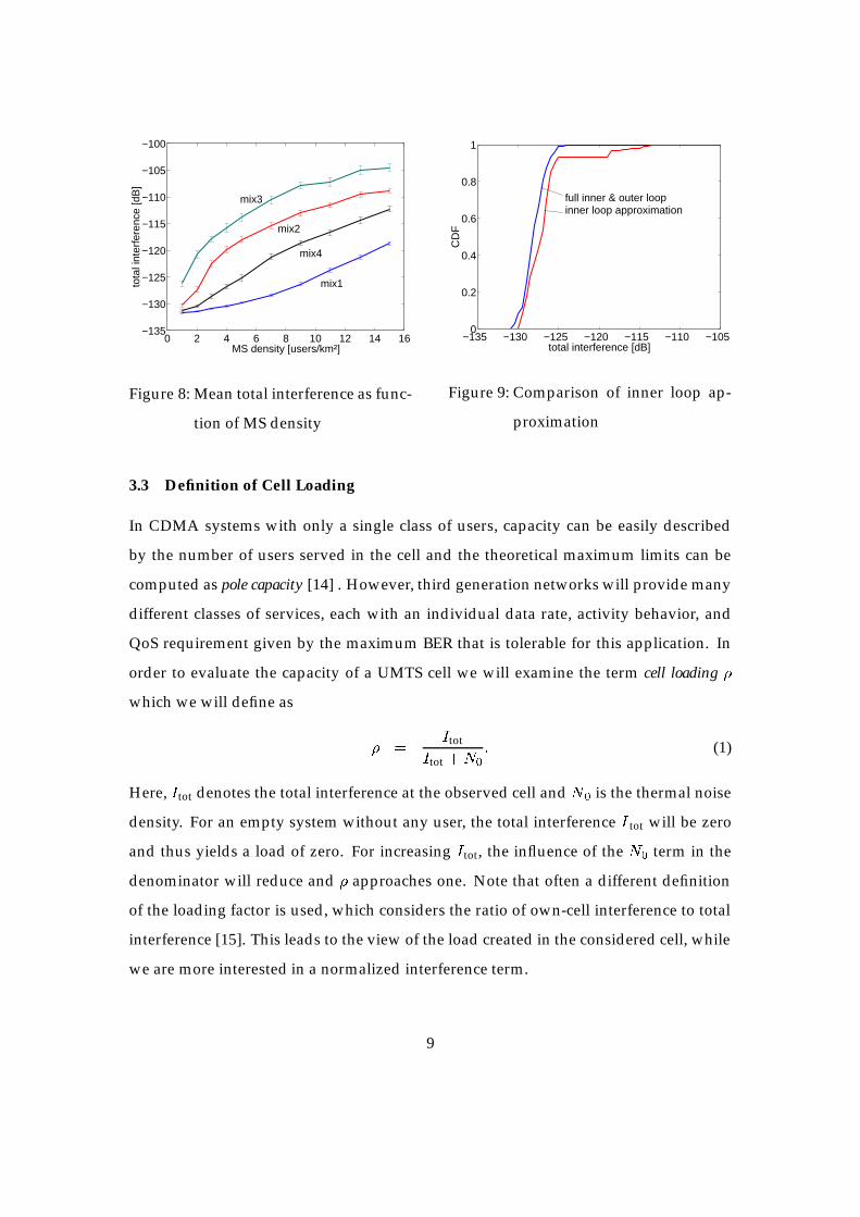
The influence of the user density on the mean total interference is illustrated in

Fig. 8. Depending on the traffic mix, the mean interference increases with the user

density, for higher data rates the increase is steeper and saturates when the user density

gets higher and the power control loops fail to achieve the target values. The outage

rate will then increase as well. The error bars in Fig. 8 give the 95% confidence interval

obtained from 30 runs.

Fig. 9 shows the CDF of the total interference power for traffic mix4, where the

full inner and outer loop simulation is compared with the inner loop approximation

described in Section 2.1. It can be seen that for low interference the approximation

matches the full loop quite well, however, for higher values the lack of the fine tuning

in the inner loop leads to a slight overestimation of the transmit power, which results

in a higher overall interference.

8

0 2 4 6 8 10 12 14 16−135

−130

−125

−120

−115

−110

−105

−100

MS density [users/km²]

tota

l int

erfe

renc

e [d

B]

mix1

mix4

mix3

mix2

Figure 8: Mean total interference as func-

tion of MS density

−135 −130 −125 −120 −115 −110 −1050

0.2

0.4

0.6

0.8

1

total interference [dB]

CD

F

full inner & outer loop inner loop approximation

Figure 9: Comparison of inner loop ap-

proximation

3.3 Definition of Cell Loading

In CDMA systems with only a single class of users, capacity can be easily described

by the number of users served in the cell and the theoretical maximum limits can be

computed as pole capacity [14] . However, third generation networks will provide many

different classes of services, each with an individual data rate, activity behavior, and

QoS requirement given by the maximum BER that is tolerable for this application. In

order to evaluate the capacity of a UMTS cell we will examine the term cell loading �

which we will define as

� =Itot

Itot +N0

: (1)

Here, Itot denotes the total interference at the observed cell and N0 is the thermal noise

density. For an empty system without any user, the total interference I tot will be zero

and thus yields a load of zero. For increasing Itot, the influence of the N0 term in the

denominator will reduce and � approaches one. Note that often a different definition

of the loading factor is used, which considers the ratio of own-cell interference to total

interference [15]. This leads to the view of the load created in the considered cell, while

we are more interested in a normalized interference term.

9

In Fig. 10 the cell loading factor is shown as a function of the MS density. It can be

seen that depending on the traffic mix, the value � describes with one value the load

caused by a certain traffic situation, regardless what traffic mix or user density exists.

Thus, a load of 0.8 could represent a load created when an average user density of 10.5

users/km2 with 12.2 kbps is considered or a density of approximately 5.5 when 75%

operate with 12.2 kbps, 20% with 144 kbps, and 5% with 384 kbps.

0 2 4 6 8 10 12 140

0.2

0.4

0.6

0.8

1

MS density [users/km²]

load

ing

fact

or

mix1 mix2mix3

mix4

inner/outerloop

inner loop approximation

Figure 10: Cell loading as function of MS density

3.4 Consideration of Outage Admission

So far, we considered that all MS would perform their power control loops regardless

of the actually received Eb=N0 of their connection. In the following we will consider the

case when users are removed from the system, whenever their outage requirements are

not fulfilled. We consider all users to be in outage, whenever their current Eb=N0 falls

below 0.5 dB under the Eb=N0 target for a period of 1 second. Since we so far modeled

all users to be active from the beginning of the simulation, we chose the following

method to remove users in outage. At first all users which exceeded the E b=N0 target

10

most were dropped and if after a recalculation of the interference situation other users

were still in outage these would be dropped step by step as well.

0 2 4 6 8 10 12 14−135

−130

−125

−120

−115

−110

MS density [users/km²]

tota

l int

erfe

renc

e [d

B]

with outage admission

without outage admission

Figure 11: Mean total interference with

outage admissions

1 3 5 7 9 11 13 150

0.2

0.4

0.6

0.8

1

MS density [users/km²]

load

ing

fact

or

without outage admission

with outage admission

Figure 12: Influence of outage admis-

sions on cell loading

In Fig. 11 and Fig. 12 the results from Section 3.2 and 3.3 for traffic mix4 are com-

pared to the case when we remove users that are over a period of 1s in outage. It can

be seen that as long as we also consider users in outage for our interference calculation

that would in reality drop their connection, we overestimate the total interference and

cell loading. In fact the removal of outage users reduces the total interference up to 10

dB and the maximum load to about 85% instead of approaching 100%.

4 EVALUATION OF COMPLEX SCENARIOS

The inner-loop approximation now enables simulations of larger scenarios with com-

plex characteristics. This section therefore demonstrates the measurement of cell pa-

rameters for a more realistic scenario. In view of network planning these results can

be used to improve the base station arrangement in order to increase the coverage and

enhance the quality of service of each user, see [2].

The scenario in this section uses data from the area around the city of Wurzburg. A

11

Figure 13: Realistic simulation scenario of the city of Wurzburg

map of this area with an extension of 6.7 � 4.2 km is illustrated in Fig. 13. We assume

that demands in teletraffic correspond to the density distribution of conventional traf-

fic, i.e. more subscribers can be found on the main streets and in the city center than

on country roads. Only mobile subscribers are used in this study. The fixed number

of subscribers is thereby distributed over the streets at the beginning of each simula-

tion. These test users move during the simulation randomly on the road system – main

streets are chosen preferably. Subscribers leaving the simulation area reenter the map

again randomly at another incoming street. The number of test users therefore remains

constant for the entire simulation time.

Contrary to the simplified studies, communication is now simulated on the basis of

calls. This means, each test user begins and ends calls randomly. Therefore, we will use

a slightly different method than in Section 3.4 to cope with outages. Since we have a

session activity in this case, not all users will begin their connection at the same time

instant. The criterion to drop outage users is given whenever the target BER can not be

reached within 2 seconds.

12

The cell of interest is cell 5, where we will focus on the highlighted sector covering

most parts of the city center with lots of streets with high density. In order to com-

pare the results to a homogeneous case, we chose also a Poisson process with the same

average number of connections in a sector. However, unlike the Poisson case, in our

Wurzburg scenario there are no stationary users.

-135 -130 -125 -120 -115 -1100

0.2

0.4

0.6

0.8

1

total interference [dB]

CD

F

mix1

mix4

Poisson processWürzburg scenario

Figure 14: CDF of total interference for mix4

In Fig. 14 the CDF of the total interference is given for traffic mix1 and mix4. It can

be recognized that for mix4 there is a difference in mean of about 3 dB which shows that

the homogeneous assumption leads to an underestimation of the total interference. For

the more homogeneous traffic of mix1 (only voice users with 12.2 kbps) a good match

between the Poisson model and the Wurzburg model can be seen. Additionally, the

inclusion of mobility in the Wurzburg scenario causes that the standard deviation of

the total interference increases by about 3 dB for mix4 and only 0.5 dB for mix1. Fig. 14

leads to the conclusion that it is possible to capture the effects of the traffic parame-

ters on the interference in a homogeneous scenario, however, in order to perform an

accurate prediction of the interference and load a detailed modeling of the location and

13

movement of the users plays an essential role.

5 CONCLUSION

In this paper we presented a simulation model for evaluating the performance of a 3G

wireless network operating with WCDMA. The capacity of such a system is greatly

influenced by the performance of the closed loop power control. We therefore modeled

the inner and outer loop uplink power control in great detail and derived empirical

distributions of the own-cell and other-cell interference. It could be seen that changing

the mix of traffic in the cells has an impact on the mean and variance of the received

interference. Furthermore, we examined the loading factor as a descriptor of the traffic

load which integrates the user density in terms of mean number of users per unit area

size and the mix of data rates into a single parameter value.

We also showed that it is important to include the user reaction to outages since this

results in calls to be dropped from not being able to maintain the Eb=N0 target level and

thus reduces the load in the cell. This also indicates the need for an accurate model of

the connection admission control mechanism implemented in the system.

The simulation time could be reduced by a factor of the inner loop updates when

we only considered the outer loop with an approximated inner loop. It could be shown

that the results were accurate enough for evaluation of the cell loading and total inter-

ference. With this approximation of the power control loops, it is possible to investigate

more complex scenarios with mobility like the real world case which we considered in

Section 4.

References

[1] F. Adachi, M. Sawahashi, and H. Suda, “Wideband DS-CDMA for next generationmobile communication systems,” IEEE Communications Magazine, Sep. 1998.

[2] U. Ehrenberger and K. Leibnitz, “Impact of clustered traffic distributions in CDMAradio network planning,” in Proc. of ITC-16, (Edinburgh, UK), June 1999.

[3] J. Zander, “Transmitter power control for co-channel interference management in

14

cellular radio systems,” in Proc. of 4th WINLAB Workshop, (New Brunswick, NJ),Oct. 1993.

[4] R. D. Yates, “A framework for uplink power control in cellular radio systems,”IEEE Journal on Sel. Areas in Comm., vol. 13, pp. 1341–1347, Sep. 1995.

[5] K. Leibnitz, P. Tran-Gia, and J. E. Miller, “Analysis of the dynamics of CDMAreverse link power control,” in Proc. of IEEE Globecom 98, (Sydney, Australia), Nov.1998.

[6] K. Leibnitz, “Impacts of power control on outage probability in CDMA wirelesssystems,” in Proc. of the 5th Int. Conf. on Broadband Communications, (Hong Kong),pp. 225–234, Nov. 1999.

[7] S. Ariyavisitakul and L. F. Chang, “Signal and interference statistics of a CDMAsystem with feedback power control,” IEEE Trans. on Comm., vol. 41, pp. 1626–1634, Nov. 1993.

[8] H. Suda, H. Kawai, and F. Adachi, “A fast transmit power control based on markovtransition for DS-CDMA mobile radio,” IEICE Trans. Commun., vol. E82-B, Aug.1999.

[9] K. Sipila, J. Laiho-Steffens, A. Wacker, and M. Jasberg, “Modeling the impact of thefast power control on the WCDMA uplink,” in Proc. of VTC’99 Spring, (Houston,TX), pp. 1266–1270, May 1999.

[10] 3GPP, “Physical layer procedures (FDD),” Report TR25.214, 3GPP, TSG RAN,2000.

[11] H. Holma and A. Toskala, WCDMA for UMTS. John Wiley & Sons, Ltd., June 2000.

[12] A. Sampath, P. S. Kumar, and J. M. Holtzman, “On setting reverse link target SIRin a CDMA system,” in Proc. of the 47th IEEE Veh. Tech. Conf., (Phoenix, AZ), May1997.

[13] 3GPP, “RF system scenarios,” Report TR25.942, 3GPP, TSG RAN WG4, Sep. 2000.

[14] V. V. Veeravalli and A. Sendonaris, “The coverage-capacity tradeoff in cellularCDMA systems,” IEEE Trans. on Veh. Tech., vol. 48, Sep. 1999.

[15] T. Ojanpera and R. Prasad, Wideband CDMA for Third Generation Mobile Communi-cations. Artech House, 1998.

15