Spring 2004

1

University of Wisconsin Madison

Department of Electrical & Computer Engineering

ECE 734 Project Report Spring 2004

Adaptation Behavior of Pipelined Adaptive Digital Filters

Gopalakrishna, Varun (varung@cae.wisc.edu)

Khanikar, Prakash (khanikar@cae.wisc.edu)

Spring 2004

2

ABSTRACT

Adaptive digital filters are difficult to pipeline due to the presence of long feedback loops, careful calibration of step size and depth of pipelining. The LMS algorithm using the stochastic gradient approach is implemented with recursive weight adaptation. However with the RLS algorithm, the resulting rate of convergence is typically an order of magnitude faster than the LMS algorithm. We implement the exponentially weighted RLS algorithm which converges in the mean square sense in about 2M iterations, where M is the number of taps in the transversal filter.

Pipelined implementation of these adaptive filters yield higher throughput, higher sample rates and low power designs. The relaxed look-ahead transformation techniques are implemented to pipeline the adaptive filters with no increase in hardware. Stability analysis for these filters are performed (with pole zero analysis) on a preliminary basis with different stages of pipelining. The above simulations are run in Matlab. With extensive literature search we present a systolic array architecture for the RLS algorithm to reduce the overhead and increase the Hardware utilization efficiency (HUE). Concurrencies/parallelism available in the computation of both these implementations are investigated and exploited with the pipelining and parallel processing techniques.

Spring 2004

3

CONTENTS

1. Adaptive Filters

1.1 Introduction .4

1.2 LMS Filters ..4

1.3 RLS Filters ...5

2. Pipelining of Adaptive Filters

2.1 Introduction

High Throughput technique ..8

2.2 Need for Pipelining: Exploiting concurrency/parallelism 8

2.3 Relaxed Look-ahead techniques .9

2.4 Specific implementations 12

2.5 Parallel processing techniques ...16

3. Systolic Arrays

3.1 Need for Systolic array implementations . 19

3.2 QRD Decomposition .. 20

3.3 QRD-RLS algorithm ......20

3.4 Dependence Graph for the QRD-RLS algorithm 21

3.5 Systolic Array implementation ..22

3.6 Scheduling ...25

4. Conclusion ......26

5. References ..27

Appendix A

Spring 2004

4

1. Adaptive Filters

1.1 Introduction

Adaptive digital filters predict a random process {y(n)} from observations of another random process {x(n)} using linear models such as digital filters. The coefficients are updated at each iteration in order to minimize the difference between filter output and the desired signal. The updating process continues until the coefficients converge. This means the weight updating is recursive.

Fig 1.1 Adaptive Filter block

Adaptive filters are used in a large number of applications including predictive speech and video compression, noise and echo cancellation, equalization, modem design, mobile radio, subscriber loops, multimedia systems, beam formers and system identification. In terms of VLSI implementation the emphasis is to reduce area or power for a specified speed and in increasing the speed of these circuits to make the systems suitable for high throughput applications. The area/power reduction is important especially in time multiplexed applications such as video and radar which demand higher speed.

1.2 LMS Filters

In the LMS algorithm, the correction applied for updating the coefficient vector is based on the instantaneous sample value of the tap-input vector and the input signal. It is dependent on the step size, the error signal e(n-1) and tap input vector u(n-1). The amplitude of the noise usually becomes smaller as the step size parameter is reduced. For all the above reasons we need to choose a well calibrated value of the step size.

With the step size suitable chosen, this algorithm updates the tap weight vector using the method of steepest descent. It is updated in accordance to the LMS algorithm that adapts to the incoming data. It is simple with no measurements of the correlation functions

Spring 2004

5

required. The LMS adaptive filter consists of an FIR filter block with the coefficient vector, input sequence and a weight update block. The design equations are outlined as follows

e(n) = d(n) - H(n).u(n) ; error estimate

(n+1) = (n) + .u(n).e*(n); weight update

The multidimensional signal flow graph of the LMS algorithm is as shown below

Fig 1.2 LMS filter block

1.3 RLS Filters

The recursive least squares algorithm (RLS) assumes the use of a transversal filter as the structural basis of the adaptive filter. This algorithm uses the method of least squares to obtain a recursive algorithm, i.e. given the least square estimate of the tap weight vector of the filter at time n-1 we may compute the updated estimate of this vector at time n upon the arrival of new data. The algorithm yields a data adaptive filter in that for each set of input data there exists a different filter. Each of the techniques to exploit parallelism in the computation is employed knowing the fact that the algorithm utilizes all the information in the input data, right from the time of the algorithm initiation stage. The resulting rate of convergence is therefore typically an order of magnitude faster than the simple LMS algorithm. However the improvement in performance is achieved at the expense of increase in computational complexity. The equations for the RLS algorithm are as outlined below. It automatically adjusts the coefficients of the tapped delay line filter without invoking initial assumptions on the statistics of the input signals.

Exponentially weighted RLS algorithm Initialize the algorithm by setting

P(0) = -1I = small positive constant

(0) = 0

For each instant of time, n = 1, 2, , Compute

Spring 2004

6

k(n) = )()1()(1

)()1(1

1

nunPnu

nunPH

; Gain vector

(n) = d(n)

H(n-1) u(n) ; true estimation error

(n) = (n-1) + k(n). *(n) ; estimate of the coefficient vector

P(n) = -1P(n-1)

-1.k(n).uH(n).P(n-1) ; update of the correlation matrix

The multidimensional signal flow graph of the RLS algorithm is as shown below

Fig 1.3 RLS filter block

Fig 1.4 Comparison of LMS and RLS techniques Factors LMS RLS

Computation method Based on the instantaneous sample

Based on past available information

Rate of convergence Low High

No of iterations 20M iterations < 2M iterations

Misadjustment Non-zero Zero

Computational Complexity Computationally simple (2M + 1) multiplications

Computationally complex (3M(3 + M)/2 multiplications

Spring 2004

7

Fig 1.4 Number of iterations in an RLS filter Fig 1.5 Number of iterations in an LMS filter

The LMS algorithm requires approximately 20M iterations to converge in mean square, where M is the number of taps in the tapped delay line filter with 2M + 1 multiplications required. The RLS algorithm however converges in the mean square in about 2M iterations, where M is the number of taps in the transversal filter. This is evident from the plots shown above.

Algorithm

The number of additions/subtractions in one iteration cycle

The number of multiplications in one iteration

cycle

Memory consumption

The number of multiplications for M = n = 64

The number of multiplications

for M = n = 1024

LMS M+1 2M 2M 8192 2.106

NLMS 2M+1 3M+50 2M 15488 3.106

FLMS 3M 10M.log2M+14M

4M 4736 0,1.106

DCT-LMS

9M 59M 3M 241664 62.106

RLS M2+M 2M2+3M+50 M2+3M 539776 134.106

FTF 5M+4 2M+151 5M+3 17856 2.106

Fig 1.6 Computational complexity of adaptive algorithms

Source: www.electronicletters.com

The complexity of an adaptive algorithm for real time operation is determined by two principal factors namely, the number of multiplications (with divisions counted as multiplications) per iteration and precision required to perform arithmetic operations. The RLS algorithm requires a total of 3M(3+M)/2 multiplications.

Spring 2004

8

2. Pipelining of Adaptive Filters

2.1 Introduction - High Throughput Technique

Pipelining is conventionally viewed as an architectural technique for increasing the throughput of an algorithm. It is technique whereby a serial algorithm G can be partitioned into (say, 2) disjoint segments G1 and G2 . If G is non-recursive then the segmentation is done by placing latches across any feed-forward cutest in the DFG representation.

In a serial algorithm, the throughput is limited by

funpipelined 21

1

GG TT

where TG1 and TG2 are the computation times of G1 and G2 respectively

With a two stage pipelined algorithm, the throughput becomes

funpipelined ),max(

1

21 GG TT

A circuit can be transformed for area-power-speed optimization using the pipelining technique. In pipelining, latches are placed at appropriate locations. This leads to reduction in the critical path. For a constant speed, the shorter critical path of the pipelined circuit can be charged or discharged with lower supply voltage which reduces the power consumption of the circuit. Another advantage of pipelining is the reduction of area in time-multiplexed applications where many computational elements can be folded into a hardware processor.

2.2 Need for Pipelining: Exploiting concurrency/parallelism

Adaptive filter structures contain feedback operations which impose an inherently sequential nature of processing or computation. Consequently they are not ideally suitable for applications that require low power or high speed or low area requirements. Techniques such as look ahead (specifically relaxed look-ahead) and others make it possible to design pipelined adaptive digital filters since the look ahead creates delays in feedback circuits which are then used for pipelining.

We identify certain algorithm-domain constraints that would guarantee implementation flexibility of algorithms designed within these constraints. For instance pipelining is a feature that allows us to trade-off speed, power and area for a VLSI implementation of DSP algorithms. The following figures show the pipelined realizations of the LMS and RLS algorithms.

Spring 2004

9

fig 2.1 Convergence characteristics of LMS filter with pipelining

The figure shows the convergence characteristics for an LMS filter for different orders of pipelining. We can clearly observe that as the order of pipelining increases, since the weight update is done only after the input is consumed (due to the introduction of latches) the error accumulates and this round off error increases for higher stages of pipelining. Similar results are seen for the RLS filters however with faster convergence rates.

fig 2.2 Convergence characteristics of RLS filter with pipelining

2.3 Relaxed Look-ahead techniques

From a single chip implementation point of view the pipelining approach holds a distinct advantage due to its lower hardware cost. Look-ahead pipelining introduces additional concurrency in serial algorithms at the expense of hardware overhead. This is because look-ahead technique transforms a serial algorithm into an equivalent pipelined one in an

Spring 2004

10

input-output sense. A direct application of look-ahead would result in a complex architecture. However change in convergence behavior is not substantial if we are ready to relax some parts of the look-ahead equations. This is relaxed look-ahead.

Relaxed look-ahead pipelining technique sacrifices the equivalence between serial and pipelined algorithms at the expense of marginally altered convergence characteristics. Thus it maintains the functionality of the algorithm rather than the input-output behavior and overall is well suited for adaptive filtering applications. In the context of adaptive filtering, the approximations can be quite crude and yet result in minimal performance loss. In almost all cases, the pipelined algorithm requires minimal hardware increase and achieves a higher throughput or requires lower power as compared to the serial algorithm.

The look-ahead technique contributes the canceling poles and zeros with equal angular spacing. The output samples can be then computed using the inputs and the delayed output sample (with M delay elements in the critical loop). We use this principle to pipeline the critical loop thereby increasing the sample rate by a factor of M. We observe that the pipelined realizations implemented require a linear increase in complexity in the number of loop pipelining stages, and are guaranteed to be stable provided that the original filter is stable. A decomposition technique is employed for the non recursive portion generated with the look-ahead process. This technique is the key in obtaining area efficient high speed VLSI implementations,

We observe the sensitivity of the pipelined RLS filters to the filter coefficients and in turn the stability of these filters with the increase in the pipelining stages. This is seen in the pole- zero plots presented as the order of pipelining is increased in the weight update loop below. We observe the filter remains stable even with higher order of pipelining provided that the original filter is stable. We do observe an outward shift in the poles of the system with very high stage of pipelining suggesting that the filters cannot be pipelined beyond this stage to achieve speed up and increased throughput. With this bound reached, pipelining can no longer increase the speed and we need to combine the parallel processing with pipelining to further increase the speed of the system which is discussed in the following sections.

Spring 2004

11

Fig 2.3 With 1st order Pipelining

Fig 2.4 With 2nd order Pipelining

Spring 2004

12

Fig 2.5 With 3rd order Pipelining

Fig 2.6 With 5th order Pipelining

2.4 Specific implementations

We look at both pipelining the RLS filter at various stages and observe the residual sum of the squares of the error to identify the various bottlenecks.

Spring 2004

13

Consider the LMS weight update equations. These represent the two recursive loops in the LMS architecture namely the weight update loop and the error feedback loop. With look-ahead transformations applied to these we get

W(n) = W(n-1) + .e(n).U(n)

= W(n-M2) + 1

0

2M

i

.e(n-i).U(n-i)

where M2 is the number of delays in the weight update loop. This transformation results in M2 latches in the weight update loop, which can be retimed to pipeline the add operation at any level. The overhead introduced by applying the look-ahead transformation directly can be reduced by applying relaxed look ahead. With delay relaxation in the error feedback loop, M1 delays are introduced

W(n) = W(n - M2) + 1

0

2M

i

e(n - M1 - i).U(n M1 - i)

With sum relaxation to further reduce the overhead leads to the following weight update

W(n) = W(n - M2) + 1'

0

2M

i

e(n - M1 - i).U(n M1 - i)

Similar principles are applied to the RLS algorithm.

Pipelining introduced

Spring 2004

14

Fig 2.7 Convergence characteristics (LMS vs RLS)

Fig 2.8 Convergence characteristics (LMS vs RLS) with 1st order pipelining

Spring 2004

15

Fig 2.9 Convergence characteristics (LMS vs RLS) with 2nd order pipelining

Figures 2.7 to 2.9 above show convergence characteristics for the LMS and the RLS filters for different orders of pipelining. Though the number of iterations for the RLS algorithm is smaller, we see the error blow up to a greater extent than for the LMS filter. This is inherently due to the recursive nature of the RLS algorithm. We see faster convergence rates for different orders of pipelining.

Fig 2.10 Pipelined RLS filter

Spring 2004

16

Fig 2.11 Pipelined RLS filter with higher order filtering

The figures above illustrate two different realizations of the pipelined RLS filter with the pipelining at different branches in the filter. Latches are introduced in the error feedback loop and the weight update block respectively. We observe that with pipelining in the FIR block leads to a higher convergence rate. With latches introduced in the weight update block we observe higher residual errors due to the fact that the weight is updated only after P clock cycles where P denotes the order of pipelining. This causes the output of the filter to deviate from the desired response.

2.5 Parallel processing techniques

To exploit concurrency in the computation of adaptive filters, we simulated a parallel processed adaptive filter scheme. Since the parallel processing and the pipelining techniques are duals of each other, we could apply the parallel processing techniques to the pipelined adaptive filters as well. To obtain a parallel processed setup, the SISO structure is converted to a MIMO structure wherein placing a latch at any line produces an effective delay of L clock cycles at the sample rate. Pipelining and parallel processing can also be combined to achieve a speedup in sample rate by a factor LxM , where L is the level of block processing and M is the pipelining stage.

There is a fundamental limit of pipelining imposed by each of the I/O bottlenecks. Hence we need to adopt a parallel processing approach, however at the cost of increase in hardware. This is a performance/hardware tradeoff. In these adaptive filters, pipelining can be used only to the extent such that the computation time is limited by the communication or I/O bound. With this bound reached, pipelining can no longer increase

Spring 2004

17

the speed and we need to combine the parallel processing with pipelining to further increase the speed of the system. Parallel processing is also used for reduction of power consumption while using slow clocks. This reduces the power consumption as compared to a pipelined system, which needs to be operated using a faster clock for equivalent throughput or sample speed.

Fig 2.12 Block Processing example

y(3k) = ax(3k) + bx(3k-1) + cx(3k-2) y(3k+1) = ax(3k) + bx(3k-1) + cx(3k-2) y(3k+2) = ax(3k+2) + bx(3k+1) + cx(3k)

The RLS filter has been block processed for a block size of 3 as shown in figure 2.12. Each of the inputs is passed through a different gain vector with individual weight updates thereby rendering a MIMO structure. This is evident from the plot which exhibits different convergence characteristics for each of the inputs. Since the parallel processing and the pipelining techniques are duals of each other, the block processing can be applied to a highly pipelined RLS filter to exploit parallelism in the computation. This is as shown in figure 2.14 which is simulated for a block size of 2. The latches are introduced in the weight update block of each of the parallel structures for a pipelined implementation.

x(3k)

Parallel system

SISO

x(n)

Sequential system

y(n)

x(3k+1)

x(3k+2) y(3k+2)

y(3k+1)

y(3k)

MIMO

Spring 2004

18

fig 2.13 Parallel processing for a RLS filter

fig 2.14 Parallel processing for a RLS filter with 1st order pipelining

Spring 2004

19

3. Systolic Arrays

3.1 Need for Systolic array implementations

These arrays are needed to represent algorithms directly by chips connected in a regular pattern. These are functional modules are arranged in a geometric lattice, each interconnected to its nearest neighbors, and common control is utilized to synchronize timing. It is different from the pipelining approaches in that it has a non-linear array structure, multi-direction data flow. Pipelining with multiprocessing at each stage of a pipeline yields the best performance . The systolic array implementation is scalable with very high throughputs. The essential difference between pipelining and the systolic approaches are the way data gets consumed.

The complexity of an adaptive algorithm for real time operation is determined by two principal factors namely, the number of multiplications (with divisions counted as multiplications) per iteration and precision required to perform arithmetic operations. To increase the overall HUE, we now propose a systolic array implementation of the RLS algorithm.

3.2 QRD Decomposition

There are a number of different algorithms for solving the least squares problem. A low power and small-area implementation needs a computationally efficient and numerically robust algorithm. In particular, square root and division require far more cycles, and thus more energy, to compute than multiply-accumulate (MAC) operations. A first order measure of the computational complexity of an algorithm can be obtained simply by counting the number and type of involved arithmetic operations as well as the data accesses required to retrieve and store the operands.

For a hardware implementation, algorithm selection criteria also need to include numerical and structural properties: robustness to finite precision effects, concurrency, regularity and locality. The unitary transformation such as the Givens Rotations are known to significantly less sensitive to round off errors and display high numerical stability.

QR decomposition (QRD) based on Givens rotations has a highly modular structure that can be implemented in a parallel and pipelined manner, which is very desirable for its hardware realization. The main tasks of the QRD are the evaluation and execution of plane rotations to annihilate specific matrix elements.

Spring 2004

20

Fig 3.1 Signal flow graph of the QR decomposition algorithm vec = vectorization; rot = rotation

The QRD block is used as a building block for Recursive least squares filters. Given a matrix , its QR-decomposition is a matrix decomposition of the form

where is an upper triangular matrix and Q is an orthogonal matrix, i.e., one satisfying

where QT is the transpose of Q and

is the identity matrix. When the QRD is used as a least square estimator, the goal is to minimize the sum of squared errors.

2

1][

|][][][|min iwnyndTi

niw

The upper triangular matrix can be calculated recursively on a sample by sample basis using the QRD- RLS algorithm based on complex Givens rotations.

3.3 QRD-RLS algorithm

This algorithm was first proposed first by Gentleman and Kung. The QRD

RLS algorithm using the triangularization process is ideal for implementation since it has good numerical properties due to the use of robust QR decomposition involving the Givens transformation and can be mapped to a coarse grain pipelining systolic array making it very suitable for VLSI implementation. Fine grain pipelining essentially can also be used to reduce the power dissipation in low to moderate speed applications. The critical period of the QRD- RLS algorithm is limited by the operation time in the recursive loop of the individual cells. To increase the speed of the algorithm, the look-ahead technique can be used. However look ahead in the above algorithm leads to increased hardware. Taking into account all the above factors, we propose a architecture for optimized performance. It is suitable for systolic array implementation which makes it interesting for real time

Spring 2004

21

applications on VLSI circuits. Among all RLS algorithms, the QRD-RLS is thus regarded as the most promising one for VLSI implementations.

In an adaptive parameter estimation setup where xT(n) is the input vector, d(n) is the reference signal and R(n) is the (N x N) is the upper triangular matrix, the QRD-RLS algorithm is summarized by

1. Initialization R(-1) = IN

_

d (-1) = .w(-1) for n = 0:L

2. )1(

)()(

)(

0

nR

nxnQ

nR

Tv

T

)1(

)()(

)(

)(_

_

1

_

nd

ndnQ

nd

ndw

v

w

e

3. w(n) = R-1(n) _

d w(n)

4. e(n) = d(n) xT(n).w(n)

3.4 Dependence Graph for the QRD-RLS algorithm

Fig 3.2 Dependence graph of the QRD-RLS algorithm

Spring 2004

22

The DG for the above algorithm has been outlined as shown. The working of the dependence graph is as follows

In the training mode, the output can be used as a convergence indicator. In the data detection mode, the block acts like a fixed filter with coefficients W on the input data Y. In the decision directed adaptation mode, the received signal used for detection needs to be applied as Y again. In the Weight flushing mode, W can be obtained by setting Y = I and D=0, in this case the output becomes 0- IW, the negated weight coefficients appear at the output one after another.

3.5 Systolic Array Implementation

We consider the case when the weight vector has three elements (M=3). The systolic array operates directly on the input data that are represented by the matrix Y and the row K. To produce an estimate of the desired response d(n), we form the inner product w(n)u(n) by post-multiplying the output of the systolic array processor by the input vector u(n). The structure below consists of two sections: a triangular systolic array and a linear systolic array. Each section of the array consists of two types of processing cells: internal and external. Each cell receives the input data for one clock cycle, and delivers the result to the neighboring cells on the next clock cycle. The triangular systolic array implements the Givens rotations part of the recursive QRD RLS algorithm and the linear section computes the least squares weight vector at the end of the entire recursion. Each cell of the triangular section stores an element of the lower triangular matrix R and is updated every clock cycle. The function of each column of PU s in this section is to rotate one column of the stored triangular matrix with a vector of data received from the left in such a way that the leading element of the received vector is annihilated. The reduced data vector is then passed on. The boundary cells compute the rotation parameters and pass them downwards on the next clock cycle. With a delay of one clock

Mode of Operation

Y D OUT Adaptation

Training Received signal

Known Sequence

Residual Error Update

Data Detection Received signal

0 Filter output -

Decision directed

adaptation

Delayed received signal

Decision signal Residual error Update

Weight Flushing

Identity Matrix 0 Filter Coefficients

-

Spring 2004

23

cycle per cell while passing the rotation parameters, the input data vectors enter the array in a skewed manner. The systolic array operates in a highly pipelined manner, wherein each vector defines a processing wave front that moves across the array. The linear section with one boundary cell and (M-1) internal cells perform the arithmetic functions. The elements of the weight vector are effectively read out backward. These operations effectively compute the RLS algorithm.

Fig 3.3 Systolic array implementation of the QRD-RLS algorithm

u(3), u(2), u(1)

u(3), u(2), 0

u(3), 0, 0

d(3), d(2), d(1)

*(1), *(2), *(3)

Linear section

Triangular section

A

B

C

Spring 2004

24

Design equations

Fig 3.4 Boundary cell

Fig 3.5 Internal cell The Dependence matrix can be deduced from the DFG as

D = 01

10 where the column matrices correspond to the Y and the K signals.

A linear schedule is defined by means of a scheduling vector s , which needs to satisfy our feasibility constraint i.e.

dT s 1 for all dependence vectors. This satisfies the causality constraint.

One possible scheduling vector which satisfies the above constraints is

sT = [ 1 1 ] , which satisfies the inequalities s1 1 and s2 1

Let us assume the projection vector dT = [0 1 ]. This condition is for resource conflict avoidance. Since the processor space vector pT and the projection vector are orthogonal, we find the processor space vector as

pTd=0 or pT = [1 0]

sTI = [1 1]j

i = i + j

If uin = 0, then X` = 22 |||||| inuX

X

X

c = 1 otherwise c = `||

||2/1

X

X

s= 0 s = `||

|||| 2

X

uXuX inin

X = X`

uin

uout = c.uin

s. 1/2X

X = s.uin + c. 1/2X X

c s

c s

uin uout

X

Spring 2004

25

Any node with index I would be executed at time i+j. Hardware utilization efficiency HUE = 1/|sTd| = 100 %

3.6 Scheduling

In an architectural implementation there is a need to find the most efficient dedicated implementation for a given problem size (i.e., fixed i, j and k). A scheduling scheme is devised to map and schedule the DG (dependence graph) onto a fixed number of parallel processing units. The task is to find the scheduling of the processors to implement the graph so as to maximize processor utilization, or equivalently, minimizing the total execution time.

PE Assignment Node mapping

pT[i j]T = [1 1 ][i j]T = i+j

Arc mapping

T

T

p

sD =

01

10

01

11 =

10

11

I/O mapping

T

T

p

s

0

0

j

i =

0

0

01

11

j

i =

i

ij

0

For discrete mapping, the SFG is projected along the diagonal so that all vectoring operations are mapped onto a single processing element. This is critical for the standard arithmetic based algorithm since the functions required for the vectoring and rotation operations are very different.

Fig 3.6 1-D discrete mapping and scheduling of QRD

Spring 2004

26

4. Conclusions

The complexity of an adaptive algorithm for real time operation is determined by two principal factors namely, the number of operations per iteration and precision required to perform arithmetic operations. These parameters are the deciding factors when designing any hardware-efficient implementation.

Pipelined adaptive filter realizations (LMS & RLS) are implemented using the relaxed look-ahead technique. The RLS filters exhibit faster convergence rates with higher order of pipelining at the cost of higher residual error and increase in computational complexity. This is a performance trade-off issue. The relax look-ahead technique results in substantial hardware savings as compared to either parallel processing or look ahead techniques. Pipelining realizations with latches introduced in the error feedback loop and the weight update block were investigated and the convergence characteristics observed. Intuitively the convergence rates with pipelining in the weight update block were higher at the cost of larger residual error due to the fact that the weight is updated only after P clock cycles where P denotes the order of pipelining. This causes the output of the filter to deviate from the desired response.

We also observe the adaptation behavior in terms of the sensitivity of the pipelined RLS filters to the filter coefficients and in turn the stability of these filters with the increase in the pipelining stages. We observe the filter remains stable even with higher order of pipelining provided that the original filter is stable. We do observe an outward shift in the poles of the system with very high stage of pipelining suggesting that the filters cannot be pipelined beyond this stage to achieve speed up and increased throughput.

There is a fundamental limit of pipelining imposed by each of the I/O bottlenecks. With this bound reached, pipelining can no longer increase the speed and we need to combine the parallel processing with pipelining to further increase the speed of the system. Hence we need to adopt a parallel processing approach, however with an increase in hardware. This is a performance/hardware tradeoff.

Owing to the hardware overhead with the look ahead techniques, we proposed a systolic array implementation based on the QRD RLS algorithm. Pipelining with multiprocessing at each stage of a pipeline yields the best performance. The systolic array implementation is scalable with very high throughputs The QR decomposition (QRD)

RLS algorithm using the triangularization process is ideal for implementation since it has good numerical properties and can be mapped to a coarse grain pipelining systolic array making it very suitable for VLSI implementation. The hardware utilization efficiency is vastly increased with the array structure. However these structures are complex and expensive.

Spring 2004

27

5. References

Bhouri, M.;Bonnet, M.;Mboup, M; A New QRD-based block adaptive algorithm ; Proceedings of the 1998 IEEE International Conference on Acoustics, Speech, and Signal Processing, 1998: Vol. 3:1497 - 1500

Haykin, S., Adaptive Filter Theory , 3rd ed. Englewood Cliffs, NJ: Prentice Hall, 1996

Lan-Da Van; Chih-Hong Chang; Pipelined RLS adaptive architecture using relaxed Givens rotations (RGR) ;. IEEE International Symposium Circuits and Systems, ISCAS 2002, Volume: 1

McWhirter, J. G.; Systolic Array for Recursive Least Squares by using Inverse Iterations ;

Mingqian T. Z.; Madhukumar A.S; Chin, Francois; QRD-RLS Adaptive equalizer and its Cordic based implementation for CDMA Systems ; International Journal on Wireless & Optical Communications, Vol 1, No 1 (2003) 25-39

Moonen, M.; Proudler, I.K.; McWhirter, J.G.; Hekstra, G.; On the formal derivation of a systolic array for recursive least squares estimation ; IEEE International Conference on Acoustics, Speech, and Signal Processing, ICASSP-94., 1994, Volume: ii ,

Ning, Zhang; Algorithm/Architecture Co-design for Wireless Communications Systems ; Berkeley publications, 2001

Parhi, K.K.; Messerschmitt, D.G.; Pipeline interleaving and parallelism in recursive digital filters. I. Pipelined incremental block filtering ; IEEE Transactions on Acoustics, Speech, and Signal Processing, Volume: 37 , Issue: 7 , July 1989

Shanbhag, N.R.; Parhi, K.K.; A pipelined LMS adaptive filter architecture ;, Conference Record of the Twenty-Fifth Asilomar Conference on Signals, Systems and Computers, 4-6 Nov. 1991

Shanbhag, N.R.; Parhi, K.K.; Pipelined adaptive DFE architectures using relaxed look-ahead ; IEEE Transactions on Signal Processing, Volume: 43 , Issue: 6 , June 1995 Pages:1368 1385

Meng,T.; Messerschmitt, D. G.; Arbitrarily high sampling rate adaptive filters ; IEEE Transcations on Acoustics, Speech, and Signal Processing, vol ASSP-35, pg 450-470

Spring 2004

28

Appendix: MATLAB codes

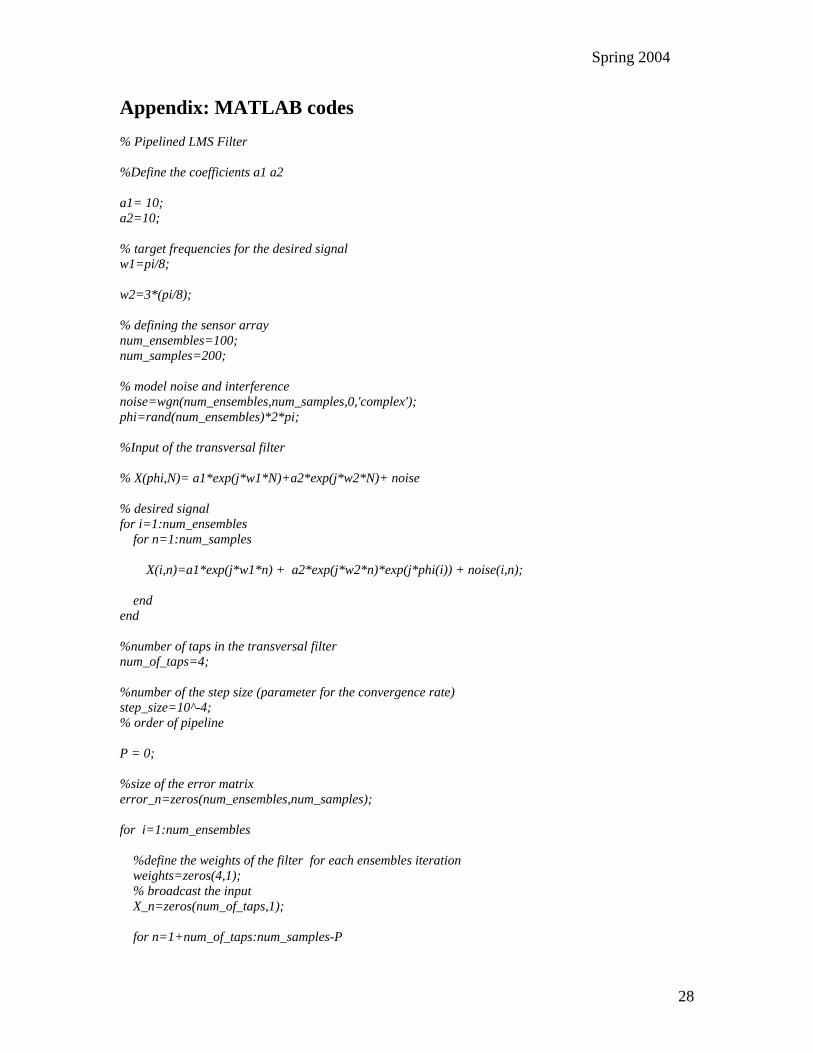
% Pipelined LMS Filter

%Define the coefficients a1 a2

a1= 10; a2=10;

% target frequencies for the desired signal w1=pi/8;

w2=3*(pi/8);

% defining the sensor array num_ensembles=100; num_samples=200;

% model noise and interference noise=wgn(num_ensembles,num_samples,0,'complex'); phi=rand(num_ensembles)*2*pi;

%Input of the transversal filter

% X(phi,N)= a1*exp(j*w1*N)+a2*exp(j*w2*N)+ noise

% desired signal for i=1:num_ensembles for n=1:num_samples X(i,n)=a1*exp(j*w1*n) + a2*exp(j*w2*n)*exp(j*phi(i)) + noise(i,n); end end

%number of taps in the transversal filter num_of_taps=4;

%number of the step size (parameter for the convergence rate) step_size=10^-4; % order of pipeline

P = 0;

%size of the error matrix error_n=zeros(num_ensembles,num_samples);

for i=1:num_ensembles %define the weights of the filter for each ensembles iteration weights=zeros(4,1); % broadcast the input X_n=zeros(num_of_taps,1); for n=1+num_of_taps:num_samples-P

Spring 2004

29

x=0; %implementation of the LMS algorithm for each iteration and each ensemble % order of pipeline for p = 0 : P % introduce appropriate latches X_n = [X(i,n-1+p);X(i,n-2+p);X(i,n-3+p);X(i,n-4+p)] ; %output for an estimated value of weights Y_n=weights'*X_n; %desired response D_n=X(i,n); %error of the filter output error_n(i,n-num_of_taps+p)=D_n-Y_n; %modified weights depending on the step size x = x+ step_size*X_n*conj(error_n(i,n-num_of_taps+p)); end % weight update weights = weights + x; end end

% mean square error for the LMS filter mean_error=zeros(300,1); for n=1:num_samples mean_error(n)=mean(error_n(:,n)); end

mean_error_lms_5= mean_error ;

% figure(1) % plot(abs((mean_error_lms_0).^2),'b'); % title(' Convergence Charecteristics of LMS Filter with Pipelining'); % grid % text(180,70,'Blue : No pipelining','FontSize',10); % text(180,80,'Red : 1st Order pipelining','FontSize',10); % text(180,90,'Yellow :2nd order pipelining','FontSize',10); % hold on % plot(abs((mean_error_lms_1).^2),'r'); % hold on; % plot(abs((mean_error_lms_2).^2),'y'); % plot(abs((mean_error_rls).^2),'r'); % text(8,30,' \leftarrow RLS','FontSize',10) % xlabel('time'); figure(2) plot(mean_error) title('No of iterations for an LMS Filter');

figure(3) plot(error_n) **********************************************************************************

Spring 2004

30

% pipelined RLS Filter

% Pipelined in the weight update loop %given -the input of the transversal filter

% X(phi,N)= a1*exp(j*w1*N)+a2*exp(j*w2*N)+ noise

%Define the coefficients a1 a2

a1= 10; a2=10;

%------------------------------- %------------------------------- % target frequencies for the desired signal

w1=pi/8; w2=3*(pi/8);

%-------------------------------

%--------------------- % defining the sensor array no_of_ensembles=200;

samples=300;

%---------------------

% model noise and interference

noise=wgn(no_of_ensembles,samples,0,'complex');

phi=rand(no_of_ensembles)*2*pi;

% desired signal for i=1:no_of_ensembles for n=1:samples X(i,n)=a1*exp(j*w1*n) + a2*exp(j*w2*n)*exp(j*phi(i)) + noise(i,n); end end %number of taps in the transversal filter numtaps=4;

% forgetting factor lambda = 0.9;

delta = 0.1;

% to hold the past values of the error correlation matrix

Spring 2004

31

ctemp= delta * eye(numtaps) ;

%number of the step size % not used in the weight update : RLS each time a different filter %step_size=10^-4;

% order of pipeline P = 0;

c=ctemp;

%size of the error matrix

error_n=zeros(no_of_ensembles,samples);

for i=1:no_of_ensembles %define the weights of the filter for each ensembles iteration weights=zeros(4,1); X_n=zeros(numtaps,1); for n=1+numtaps:samples-P temp=0; ctemp=c; %implementation of the LMS algorithm for each iteration and each ensemble % for pipeline order P for p = 0 : P % Broadcast input X_n = [X(i,n-1+p);X(i,n-2+p);X(i,n-3+p);X(i,n-4+p)] ; %output for an estimated value of weights Y_n=weights'*X_n; %desired response D_n=X(i,n); % to reduce the cost %1 x = (1/lambda) * ctemp * X_n; % compute k %2 k = (1/(1+ X_n'*x))*x; k = ((1/lambda) * ctemp * X_n) / (1 + (1/lambda) * X_n' * ctemp * X_n);

% compute correlation matrix temp1 = (1/lambda * k * X_n' * ctemp); %3 c = (1/lambda) * ctemp - k*x';

Spring 2004

32

c = (1/lambda * ctemp) - temp1; %error of the filter output error_n(i,n-numtaps+p)=D_n-Y_n; %modified weights temp = temp+ k*conj(error_n(i,n-numtaps+p)); end % weight update weights = weights + temp; end end

% mean square error for the RLS filter mean_error=zeros(300,1); for n=1:samples mean_error(n)=mean(error_n(:,n)); end

mean_error_rls_1 = mean_error;

% plot(abs((mean_error_rls_1).^2),'b'); % title(' Pipelined RLS Filter (with higher order pipelining)'); % grid % text(180,70,'Blue : Pipelining in the weight update loop','FontSize',10); % text(180,80,'Red : Pipelining in the FIR block','FontSize',10); % % text(180,90,'Yellow :2nd order pipelining','FontSize',10); % hold on % plot(abs((mean_error_rls_2).^2),'r'); % hold on; % plot(abs((mean_error_rls_2).^2),'y'); figure(1) plot(abs((mean_error).^2));

figure(2)

plot(mean_error) title('No of iterations for an RLS Filter');

figure(3) plot(error_n)

**********************************************************************************

Spring 2004

33

**********************************************************************************

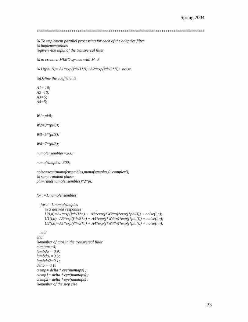
% To implement parallel processing for each of the adaptive filter % implementations %given -the input of the transversal filter

% to create a MIMO system with M=3

% U(phi,N)= A1*exp(j*W1*N)+A2*exp(j*W2*N)+ noise

%Define the coefficients

A1= 10; A2=10; A3=5; A4=5;

W1=pi/8;

W2=3*(pi/8);

W3=5*(pi/8);

W4=7*(pi/8);

numofensembles=200;

numofsamples=300;

noise=wgn(numofensembles,numofsamples,0,'complex'); % same random phase phi=rand(numofensembles)*2*pi;

for i=1:numofensembles for n=1:numofsamples % 3 desired responses U(i,n)=A1*exp(j*W1*n) + A2*exp(j*W2*n)*exp(j*phi(i)) + noise(i,n); U1(i,n)=A3*exp(j*W3*n) + A4*exp(j*W4*n)*exp(j*phi(i)) + noise(i,n); U2(i,n)=A1*exp(j*W2*n) + A4*exp(j*W4*n)*exp(j*phi(i)) + noise(i,n); end end %number of taps in the transversal filter numtaps=4; lambda = 0.9; lambda1=0.5; lambda2=0.1; delta = 0.1; ctemp= delta * eye(numtaps) ; ctemp1= delta * eye(numtaps) ; ctemp2= delta * eye(numtaps) ; %number of the step size

Spring 2004

34

step_size=10^-4; % order of pipeline P = 1; c=ctemp; c1=ctemp1; c2=ctemp2;

%size of the error matrix

error_n_r=zeros(numofensembles,numofsamples); error_n_r_1=zeros(numofensembles,numofsamples); error_n_r_2=zeros(numofensembles,numofsamples);

for i=1:numofensembles %-------------------------------------------------------------- %define the weights of the filter for each ensembles iteration weights=zeros(4,1); weights_1=zeros(4,1); weights_2=zeros(4,1); U_n=zeros(numtaps,1); U_n_1 = zeros(numtaps,1); U_n_2 = zeros(numtaps,1); %-------------------------------------------------------------- for n=1+numtaps:numofsamples-P temp=0; temp1=0; temp2=0; %implementation of the LMS algorithm for each iteration and each ensemble for p = 0 : P ctemp=c; ctemp1=c1; ctemp2=c2;

U_n = [U(i,n-1+p);U(i,n-2+p);U(i,n-3+p);U(i,n-4+p)] ; U_n_1 = [U1(i,n-1+p);U1(i,n-2+p);U1(i,n-3+p);U1(i,n-4+p)] ; U_n_2 = [U2(i,n-1+p);U2(i,n-2+p);U2(i,n-3+p);U2(i,n-4+p)] ; %---------------------------------------- %output for an estimated value of weights Y_n=weights'*U_n; Y_n_1= weights_1'*U_n_1; Y_n_2= weights_2'*U_n_2; %---------------------------------------- %desired response D_n=U(i,n); % different gain vectors for each of the inputs k = ((1/lambda) * ctemp * U_n) / (1 + (1/lambda) * U_n' * ctemp * U_n); k1 = ((1/lambda1) * ctemp1 * U_n_1) / (1 + (1/lambda1) * U_n_1' * ctemp1 * U_n_1);

Spring 2004

35

k2 = ((1/lambda2) * ctemp2 * U_n_2) / (1 + (1/lambda2) * U_n_2' * ctemp2 * U_n_2); % compute correlation matrix %3 c = (1/lambda) * ctemp - k*x'; c = (1/lambda * ctemp) - (1/lambda * k * U_n' * ctemp); c1 = (1/lambda1 * ctemp1) - (1/lambda1 * k1 * U_n_1' * ctemp1); c2 = (1/lambda2 * ctemp2) - (1/lambda2 * k2 * U_n_2' * ctemp2); %error of the filter output error_n_r(i,n-numtaps+p)=D_n-Y_n; error_n_r_1(i,n-numtaps+p)=D_n-Y_n_1; error_n_r_2(i,n-numtaps+p)=D_n-Y_n_2; %modified weights depending on the step size temp = temp+ k*conj(error_n_r(i,n-numtaps+p)); temp1 = temp1+ k1*conj(error_n_r_1(i,n-numtaps+p)); temp2 = temp2+ k2*conj(error_n_r_2(i,n-numtaps+p)); end weights = weights + temp; weights_1 = weights_1 + temp1; weights_2 = weights_2 + temp2; end end

error_mean_r=zeros(300,1); for n=1:numofsamples error_mean_r(n)=mean(error_n_r(:,n)); end

%e1=error_mean_r; % error_mean_r1=zeros(300,1); for n=1:numofsamples error_mean_r1(n)=mean(error_n_r_1(:,n)); end %e2=error_mean_r1;

% error_mean_r2=zeros(300,1); for n=1:numofsamples error_mean_r2(n)=mean(error_n_r_2(:,n)); end

e3=error_mean_r2;

plot(abs((e1).^2),'b');

Spring 2004

36

xlabel('time'); ylabel('mean square error'); title('Parallel processing for a RLS Filter (with 1st order pipelining)'); grid

*********************************************************************************** % pipelined RLS filter

% latches introduced in the FIR block %Define the coefficients a1 a2:

a1= 10;

a2=10;

w1=pi/8;

w2=3*(pi/8); ensembles=200; s=300;

noise=wgn(ensembles,s,0,'complex');

phi=rand(ensembles)*2*pi;

% U(phi,N)= a1*exp(j*W1*N)+a2*exp(j*w2*N)+ noise

for i=1:ensembles for n=1:s U(i,n)=a1*exp(j*w1*n) + a2*exp(j*w2*n)*exp(j*phi(i)) + noise(i,n); end end

%number of taps in the transversal filter numtaps=4; lambda = 0.9; delta = 0.1; ctemp= delta * eye(numtaps) ;

%number of the step size step_size=10^-4;

% order of pipeline P = 1; c=ctemp;

%size of the error matrix

error_n=zeros(ensembles,s);

Spring 2004

37

for i=1:ensembles %-------------------------------------------------------------- %define the weights of the filter for each ensembles iteration weights=zeros(4,1); U_n=zeros(numtaps,1); %-------------------------------------------------------------- for n=1+numtaps:s-P temp=0; %implementation of the LMS algorithm for each iteration and each ensemble for p = 0 : P ctemp=c; U_n = [U(i,n-1+p);U(i,n-2+p);U(i,n-3+p);U(i,n-4+p)] ; %---------------------------------------- %output for an estimated value of weights Y_n=weights'*U_n; %---------------------------------------- %desired response D_n=U(i,n); % to reduce the cost %1 x = (1/lambda) * ctemp * U_n; % compute k %2 k = (1/(1+ U_n'*x))*x; k = ((1/lambda) * ctemp * U_n) / (1 + (1/lambda) * U_n' * ctemp * U_n); if (p==0) k_prev = k; else if (p==P) k_prev = k; end end % compute correlation matrix temp1 = (1/lambda * k_prev * U_n' * ctemp); %3 c = (1/lambda) * ctemp - k*x'; c = (1/lambda * ctemp) - temp1; %error of the filter output error_n(i,n-numtaps+p)=D_n-Y_n; %modified weights depending on the step size temp = temp+ k_prev*conj(error_n(i,n-numtaps+p)); end %k_prev=k; weights = weights + temp;

Spring 2004

38

end end

mean_error=zeros(300,1); for n=1:s mean_error(n)=mean(error_n(:,n)); end

mean_error_rls_2 = mean_error;

% plot(abs((mean_error).^2),'b'); % title(' Convergence Analysis (With 2nd order pipelining)'); % grid % text(130,78,'Blue : Pipelined in Feedback loop','FontSize',10); % hold on % plot(abs((error_mean_r).^2),'r'); % text(130,70,'Red : Pipelined in Weight update loop','FontSize',10) % xlabel('time'); % % % figure(2) % % plot(mean_error) % % figure(3) % plot(error_n)

**********************************************************************************

This document was created with Win2PDF available at http://www.daneprairie.com.The unregistered version of Win2PDF is for evaluation or non-commercial use only.