SEMANTIC HASHING

Ruslan Salakhutdinov and Geoffrey HintonUniversity of Toronto, Machine Learning Group

IRGM Workshop

July 2007

1

Existing Methods

• One of the most popular and widely used in practice algorithmsfor document retrieval tasks is TF-IDF. However:– It computes document similarity directly in the word-count space, which

can be slow for large vocabularies.– It assumes that the counts of different words provide independent

evidence of similarity.– It makes no use of semantic similarities between words.

• To overcome these drawbacks, models for capturinglow-dimensional, latent representations have been proposed andsuccessfully applied in the domain of information retrieval.

• One such simple and widely-used method is Latent SemanticAnalysis (LSA), which extracts low-dimensional semanticstructure using SVD to get a low-rank approximation of theword-document co-occurrence matrix.

2

Drawbacks of Existing Methods

• LSA is a linear method so it can only capture pairwisecorrelations between words. We need something more powerful.

• Numerous methods, in particular probabilistic versions of LSAwere introduced in the machine learning community.

• These models can be viewed as graphical models in which asingle layer of hidden topic variables have directed connectionsto variables that represent word-counts.

• There are limitations on the types of structure that can berepresented efficiently by a single layer of hidden variables.

• Recently, Hinton et al. have discovered a way to perform fast,greedy learning of deep, directed belief nets one layer at a time.

• We will use this idea to build a network with multiple hiddenlayers and with millions of parameters and show that it candiscover latent representations that work much better.

3

Learning multiple layers

W

W

W

W

RBM500

1

RBM

2

500

500

500

32

RBM

RBM

3

4

30

500

• A single layer of features generally cannotperfectly model the structure in the data.

• We will use a Restricted BoltzmannMachine (RBM), which is a two-layer undirectedgraphical model, as our building block.

• Perform greedy, layer-by-layer learning:– Learn and Freeze W1

– Treat the learned RBM features, driven bythe training data as if they were data.

– Learn and Freeze W2.– Greedily learn as many layers of features

as desired. .

• Each layer of features captures stronghigh-order correlations between the activitiesof units in the layer below.

4

RBM for count data

i

j

W

v

h

bias

• Hidden units remain binary and the visibleword counts are modeled by the ConstrainedPoisson Model.

• The energy is defined as:E(v,h) = −

∑

i bivi −∑

j bjhj −∑

i,j vihjwij

+∑

i vi log ZN

+∑

i log Γ(vi + 1)

• Conditional distributions over hidden and visible units are:

p(hj = 1|v) =1

1 + exp(−bj −∑

i wijvi)

p(vi = n|h) = Poisson(

exp (λi +∑

j hjwij)∑

k exp(

λk +∑

j hjwkj

)N

)

• where N is the total length of the document.

5

The Big Picture

W

W

W +ε

W +ε

W +ε

W

W +ε

W +ε

W +ε

20001

2

500

2000

1 1

2 2

500

500

GaussianNoise

500

3 3

2000

500

500RBM

500

500RBM

3

RBM

Recursive Pretraining Fine−tuning

2

1

3 4

5

6

Code Layer

32

32

T

T

T

6

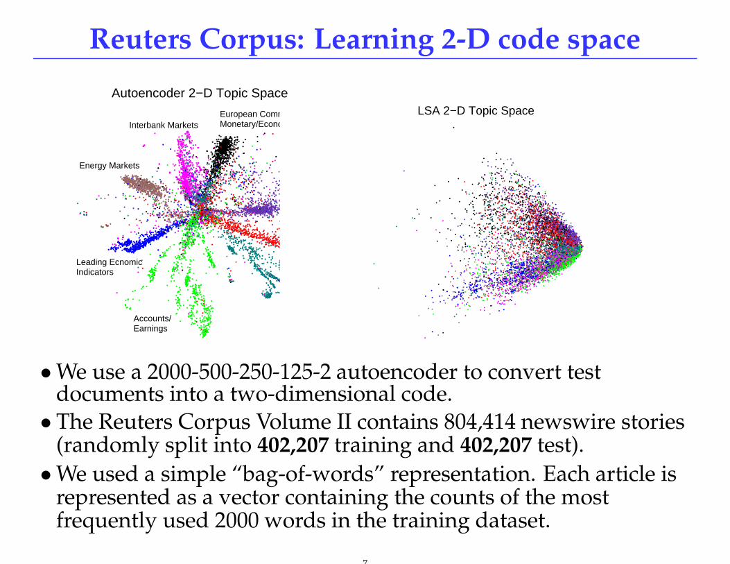
Reuters Corpus: Learning 2-D code space

Autoencoder 2−D Topic Space

Legal/JudicialLeading Ecnomic Indicators

European CommunityMonetary/Economic

Accounts/Earnings

Interbank Markets

Government Borrowings

Disasters andAccidents

Energy Markets

LSA 2−D Topic Space

• We use a 2000-500-250-125-2 autoencoder to convert testdocuments into a two-dimensional code.

• The Reuters Corpus Volume II contains 804,414 newswire stories(randomly split into 402,207 training and 402,207 test).

• We used a simple “bag-of-words” representation. Each article isrepresented as a vector containing the counts of the mostfrequently used 2000 words in the training dataset.

7

Results for 10-D codes

• We use the cosine of the angle between two codes as a measure ofsimilarity.

• Precision-recall curves when a 10-D query document from the testset is used to retrieve other test set documents, averaged over402,207 possible queries.

0.1 0.2 0.4 0.8 1.6 3.2 6.4 12.8 25.6 51.2 100

10

20

30

40

50

Recall (%)

Pre

cisi

on

(%

)

Autoencoder 10DLSA 10DLSA 50DAutoencoder 10Dprior to fine−tuning

8

Semantic Hashing

W

W

W +ε

W +ε

W +ε

W

W +ε

W +ε

W +ε

20001

2

500

2000

1 1

2 2

500

500

GaussianNoise

500

3 3

2000

500

500RBM

500

500RBM

3

RBM

Recursive Pretraining Fine−tuning

2

1

3 4

5

6

Code Layer

32

32

T

T

T

• Learn to map documents into semantic 32-D binary code and usethese codes as memory addresses.

• We have the ultimate retrieval tool: Given a query document,compute its 32-bit address and retrieve all of the documentsstored at the similar addresses with no search at all.

9

The Main Idea of Semantic Hashing

SemanticallySimilarDocuments

Memory

Document

f

10

Semantic HashingReuters 2−D Embedding of 20−bit codes

Accounts/Earnings

Government Borrowing

European Community Monetary/Economic

Disasters and Accidents

Energy Markets

0.1 0.2 0.4 0.8 1.6 3.2 6.4 12.8 25.6 51.2 100 0

10

20

30

40

50

Recall (%)

Pre

cisi

on

(%

)

TF−IDFTF−IDF using 20 bitsLocality Sensitive Hashing

• We used a simple C implementation on Reuters dataset (402,212training and 402,212 test documents).

• For a given query, it takes about 0.5 milliseconds to create ashort-list of about 3,000 semantically similar documents.

• It then takes 10 milliseconds to retrieve the top few matches fromthat short-list using TF-IDF, and it is more accurate than fullTF-IDF.

• Locality-Sensitive Hashing takes about 500 milliseconds, and isless accurate. Our method is 50 times faster than the fastestexisting method and is more accurate.

11