university of massachusetts department of civil and

UNIVERSITY OF MASSACHUSETTS Department of Civil and AMHERST Environmental Engineering

233 Marston Hall voice: 413.545.0349 130 Natural Resources Road Amherst, MA 01003-9293 http://www.cee.umass.edu/

The University of Massachusetts is an Affirmative Action/Equal Opportunity Institution

State University of Maringá, Maringá-PR, Brazil To Whom it May Concern, It was a pleasure to have the opportunity to work with Dr. Rafael Alves de Souza for the period between March 01, 2015 and June 30, 2015 during his visit to the Department of Civil and Environmental Engineering at the University of Massachusetts Amherst. Dr. Alves de Souza participated in various scholarly activities throughout his stay and performed research activities that have helped to establish and promote the collaboration between our two universities. On March 27, 2015 Dr. Alves de Souza delivered the talk “Structural Failures: Learning from the Errors” for the graduate student seminar in Structural Engineering and Mechanics. This seminar series is a fundamental educational component for graduate students in our group. The general topic of Dr. Alves de Souza’s investigations while on visit at UMass Amherst was in the area of "Assessment of the Behavior of Selected Complex Reinforced Concrete Structures Using Nonlinear Analysis”. Dr. Alves de Souza developed nonlinear finite element models for various problems involving discontinuity regions in structural concrete components. These elements were tested in the structural engineering laboratory at the University of Massachusetts so they provided a good opportunity for validation of the models. The first of these series of problems involved modeling reinforced concrete coupling beams under cyclic load reversals. Coupling beams are typically short and deep members that suffer from severe stiffness degradation after first cracking. The degradation that ensues upon cycling is a challenging modeling problem. Dr. Alves de Souza studied the nuances of earthquake engineering related to coupling beams and developed models that capture the backbone (envelope response) of these components that are used in coupled wall systems for medium to tall buildings. During Dr. Alves de Souza’s visit to UMass, an opportunity arose to model a very deep concrete beam that was about to be tested at the University of Toronto, Canada. A call to develop predictions of strength and deflection of this very deep beam was sent by the researchers from Toronto so we decided to participate in the competition. The entry included predictions using nonlinear finite element analyses as well as the modified compression field theory.

Finally, Dr. Alves de Souza also modeled a series of deep beams with longitudinal bars containing short anchorage length that were tested at UMass a few years ago. The models included the secondary reinforcement (shrinkage and temperature) that was built into the beams. They also concentrated on modeling the anchorage of longitudinal reinforcement to reflect the as-built conditions. As part of this research a paper was prepared and submitted to IBRACON that highlights the importance of including secondary reinforcement in models. The paper further points to the conservativeness of current design procedures when using strut-and-tie models in the Brazilian Code NBR6118.

UNIVERSITY OF MASSACHUSETTS Department of Civil and AMHERST Environmental Engineering

233 Marston Hall voice: 413.545.0349 130 Natural Resources Road Amherst, MA 01003-9293 http://www.cee.umass.edu/

The University of Massachusetts is an Affirmative Action/Equal Opportunity Institution

I believe that Dr. Alves de Souza’s visit to UMass has been very productive and has fostered the start of future collaborations between our universities. The work he conducted while on stay at UMass will likely result in additional publications that will be prepared after Dr. Alves de Souza returns to Brazil. I certainly look forward to continue future collaborations in the field of modeling structural concrete members with Dr. Alves de Souza. Sincerely,

Sergio F. Breña, Ph.D. Coordinator, Structural Engineering and Mechanics Group Civil and Environmental Engineering [email protected]

Research Project (Post-Doc)

"Assessment of the Behavior of Selected Complex Reinforced

Concrete Structures Using Nonlinear Analysis"

Coordinator: Dr. Rafael Alves de Souza

State University of Maringá (Brazil)

Supervisor: Dr. Sergio Breña

University of Massachusetts Amherst (USA)

Amherst, Massachusetts

March to June 2015

2

“If a civil engineer is to acquire fruitful

experience in a brief span of time, expose him to the concepts of earthquake engineering, no matter

if he is later not to work in earthquake country.”

Nathan M. Newmark and Emilo Rosenbleuth

3

SUMARY

Abstract 5

1. INTRODUCTION 6

2. RESEACH SIGNIFICANCE 9

3. OBJECTIVES 10

4. SHEAR-WALL-FRAME BUILDINGS 11

4.1 Distribution of Walls in a Building Floor Plan 11

4.2 Analysis of Shear-Wall-Frame Buildings 16

5. DESIGN OF COUPLING BEAMS 21

5.1 Equilibrium Relationships 21

5.2 Failure Modes 22

5.3 Reinforcement Layout for Coupling Beams 25

6. EXPERIMENTAL RESULTS: AMHERST COUPLING BEAMS 27

6.1 General Description of the Experimental Research 27

6.2 Behavior of the Specimen CB-1 30




7. SIMULATIONS OF THE TESTED COUPLING BEAMS 40

7.1 Shear Forces and Bending Moments in the Coupling Beams 40

7.2 Chord Rotation in the Coupling Beams 41

7.3 Predictions Using Analytical Models 43

7.3.1 ACI-318, ASCE/SEI 41-06, FEMA 356 and FEMA 306 43

7.3.2 Strut-and-Tie Model and Stress Fields 55

7.4 Predictions Using Numerical Models 72

7.4.1 Predictions Using RESPONSE 2000 72

7.4.2 Predictions Using ATENA2D 75

7.4.3 Pushover Analysis Using SAP2000 90

7.4.4 Comparisons Among the Obtained Results 106

8. DEEP BEAMS 107

8.1 Introduction 107

8.2 Amherst's Experimental Results 109

8.2.1 General Description 109

8.2.2 Specimen DB1.0-1.00 111

8.2.3 Specimen DB1.0-0.75 112

4

8.2.4 Specimen DB1.0-0.50 112

8.2.5 Specimen DB1.0-0.32 113

8.2.6 Specimen DB1.0-0.75L 113

8.2.7 Specimen DB1.0-0.28L 114

8.2.8 Specimen DB1.5-0.75 114

8.2.9 Specimen DB1.5-0.50 115

8.2.10 Specimen DB1.5-0.38 115

8.2.11 Specimen DB2.0-0.75 116

8.2.12 Specimen DB2.0-0.50 116

8.2.13 Specimen DB2.0-0.43 117

8.3. Specimen Deflections 117

8.4 Analytical Analysis Using Strut-and-Tie Model 119

8.5 Nonlinear Analysis Using ATENA2D 129

9. PREDICTION CONTEST OF A STRIP BEAM (UNIVERSITY OF TORONTO) 139

10. CONCLUSIONS 147

11. REFERENCES 150

APPENDIX A - Strut-and-Tie Model for the Deep Beams Tested by ROY (2006) 157

5

ABSTRACT

Analysis of reinforced concrete structures subjected to static or geometric discontinuities ("D Regions") using nonlinear finite element analysis is nowadays one of the best tools for assessing the behavior of complex structures. Despite the qualities of this approach that can be seen as a powerful virtual laboratory, some issues need to be better investigated in order to evaluate the performance of the available constitutive models. When applying nonlinear finite element analysis to structural concrete, there is a general preference for using perfect bond and static loading as the majority of the problems can be very well simulated using this assumptions. In this way, the present research project aims at applying nonlinear analysis enhanced by more refined procedures as bond models and cyclic loading for simulating some shear dominant reinforced concrete structures. Experimental results obtained at the University of Massachusetts Amherst for coupling beams and deep beams were selected for this purpose and were investigated using the nonlinear analysis resources available in some different package software. The experimental results were also compared with analytical results obtained using code-based equations and special developed strut-and-tie models. Based on the background obtained during this research, the present report also explores the results submitted to a contest prediction of a huge strip beam occurred at the University of Toronto. The obtained results revealed that predicting shear behavior of reinforced concrete structures is still a great challenge for structural engineers worldwide.

Keywords: Structural Concrete, D Regions, Nonlinear Analysis, Stress Fields and Strut-and-Tie Models.

RESUMO

A análise de estruturas submetidas a descontinuidades estáticas ou dinâmicas ("Regiões D") por intermédio dos recursos de análise não-linear disponibilizados através do Método dos Elementos Finitos é hoje uma das melhores ferramentas para se avaliar o comportamento de estruturas complexas em concreto estrutural. A despeito das qualidades dessa abordagem, que pode ser interpretada como um verdadeiro laboratório virtual, alguns aspectos precisam ser melhor investigados de maneira a se avaliar a performance dos modelos constitutivos disponíveis atualmente. Observa-se que a utilização da análise não-linear tem sido empregada na maioria dos casos, através da adoção de modelos constitutivos que consideram a aderência perfeita das armaduras com o concreto sujeita a carregamentos estáticos, uma vez que a adoção dessas condições representa uma gama muito grande de problemas em concreto estrutural. Dessa maneira, o presente projeto de pesquisa tem por objetivo a aplicação de recursos de análise não-linear com características mais avançadas tais como modelos de aderência entre concreto e armaduras e modelo incremental de carregamento considerando ações cíclicas. Resultados experimentais obtidos na University of Massachusetts Amherst para vigas de conexão de paredes ("coupling beams") e vigas-parede ("deep beams") foram selecionados para esse propósito e foram investigados utilizando os recursos de análise não-linear de diferentes programas selecionados. Os resultados experimentais selecionados também foram comparados com resultados analíticos baseados em equações disponíveis em códigos normativos e modelos de escoras e tirantes especialmente desenvolvidos para os problemas selecionados. Levando em conta o conhecimento adquirido durante a pesquisa, o presente relatório apresenta ainda os resultados submetidos para uma competição ocorrida na Universidade de Toronto para uma viga de dimensões impressionantes. Os resultados obtidos revelam que a previsão do comportamento de estruturas de concreto

dominadas por cisalhamento ainda é um grande desafio para os engenheiros estruturais mundo afora.

Palavras-Chave: Concreto estrutural, Regiões D, Análise Não-Linear, Campos de Tensão e Modelos de Escoras e Tirantes.

6

1. INTRODUCTION

Since the remote years of developing of reinforcement concrete structures it is well known that concrete has deficiencies for absorbing tensile stresses. In this way, since the first approaches, concrete is used for absorbing compressive stresses and metallic reinforcements are used even for tensile or compressive stresses. This model was first introduced by RITTER (1899) and was later enhanced by MÖRSCH (1908), in a way that this model is usually referred as "Ritter and Mörsch Truss Model" or "Truss Analogy" in the

literature.

The "Truss Analogy" was deeply studied during the 60's and 70's, and its generalization was denominated as "Strut-and-Tie Models" based on extensive research conducted at the University of Stuttgart by LEONHARDT & MÖNNING (1977, 1978), SCHLAICH et al. (1987) and SCHÄFER & SCHLAICH (1991). It must be mentioned that "Strut-and-Tie Models" were first developed based on equilibrium equations, taking into account forces estimated in the struts and ties before concrete cracking, i.e., based on elastic analysis using the Theory of Elasticity. This approach is nowadays recommended by many structural codes worldwide for design of "D Regions" as for example CEB-FIP Model Code 1990 (1993), CSA (1994), EHE (1999), ACI-318 (2008) and NBR6118 (2014).

At the same period, independent researchers developed in the universities of Zürich and Copenhagen an alternative approach based on the Theory of Plasticity. This alternative approach was denominated "Stress Fields Method" and has its background based on the work published by DRUCKER (1961), THÜRLIMANN et al (1975 e 1983), NIELSEN et al (1978), MARTI (1980), MUTTONI et al (1997), RUIZ & MUTTONI (2007),

KOSTIC (2009) and MUTTONI et al (2011).

In fact, "Strut-and-Tie Models" may be assumed as discrete representations (resultants) of "Stress Fields Models" in a way that both methods may be considered complementary approaches. While "Strut-and-Tie Models" takes into account equilibrium conditions based on elastic analysis, "Stress Fields Models" usually assumes equilibrium conditions based on the assumption of a rigid-plastic stress-strain law without tensile strength for the concrete (in contrast to the linear elastic uncracked law on which the analyses of SCHLAICH

et al (1987) are based).

According to RUIZ & MUTTONI (2007), neglecting the tensile strength of concrete requires placing a minimal amount of reinforcement for crack control to ensure a satisfactory behavior of the structure. This reinforcement ensures that no brittle failure occurs at cracking and that the cracks are suitably smeared over the element at the serviceability limit state. Taking into account this philosophy RUIZ & MUTTONI (2007) developed the package software jConc (http://i-concrete.epfl.ch), a platform where the concrete stress-strain response is considered elastic-perfectly plastic in compression and the tensile strength of the concrete is neglected. By another hand, the behavior of the reinforcement steel is modeled by a uniaxial response

(neglecting dowel action) with a bilinear elasto-plastic law with strain hardening.

7

"Stress Field Models" combined with the finite element method and elastic-perfectly plastic behavior for the materials may provide a very good approach once the minimum mesh reinforcement usually required by the structural codes is introduced in the simulations. Despite the qualities of jConc for simulating reinforced/prestressed concrete structures using "Stress Fields", especially "D Regions", bond between reinforcement and concrete is not considered explicitly, as in this kind of stress field approach, concrete and steel act in an independently way, i.e., if no sufficient steel is provided in the tensile regions this approach will fail. In this way, this approach is good to identify the mechanisms of resistance of a structure but may be inefficient if anchorage issues or concrete contribution for tension is to be evaluated.

In order to simulate reinforced concrete structures in a more complete way some additional considerations must be made. Nonlinear analysis taking into account, for example, the tensile strength of the concrete and the bond-slip behavior between concrete and the reinforcement may provide more refined results in order to

enhance the available analytical models.

A more robust nonlinear analysis can be applicable even to predict the ultimate limit state as well as to forecast the service limit state, contributing for the production of more economical and safer structures. Another great advantage of the nonlinear analysis is to provide an estimative of strength for damaged structures or structures which need to be strengthened for some reason. However, one should recognize that the number of parameters necessary for this kind of simulation will considerably increase when compared with a simpler approach as that provided in jConc.

Nonlinear analysis using perfect bond is a very common approach and there are many numerical results available in the literature in this field, some of them produced by the proponent of this proposal (SOUZA & BITTENCOURT (2006), SOUZA et al (2007), SOUZA (2008), SOUZA et al (2009), SOUZA et al (2010), SOUZA (2010)). By another hand, nonlinear analysis using bond models and cyclic loading are less common

and will be among the objectives of this research.

For this purpose, the package software ATENA 2D was selected to be used in this research proposal, taking into account the good performance already observed in previous simulations considering perfect bond and static loading. For modeling the concrete behavior, a fracture-plastic model based on the classical orthotropic smeared crack formulation implemented by CERVENKA & CERVENKA (2003, 2005) was selected. Reinforcements were modeled using an embedded formulation and different solution methods based on the

“Newton-Raphson Method” and “Arc Length Method” were applied for the solution scheme.

The basic property of the reinforcement bond model in the ATENA 2D is the bond-slip relationship. This relationship defines the bond strength depending on the value of current slip between reinforcement and surrounding concrete. ATENA 2D contains three bond-slip models: according to the CEB-FIB Model Code (1990), slip law by BIGAJ (1999) and the user defined law. In the first two models, the laws are generated based on the concrete compressive strength, reinforcement diameter and reinforcement type. Other package software like SAP2000 and RESPONSE2000 were also applied in some simulations.

8

One selected problem to be investigated using ATENA2D in this project was the behavior and strength of coupling beams subjected to seismic actions tested by IHTIYAR (2006). In this research, the behavior of four large-scale specimens, representing walls joined by a coupling beam were tested at the University of Massachusetts Amherst. The behavior of the coupling beams was previously simulated numerically by BREÑA et al (2009, 2010) using jConc and despite the good results regarding the ultimate load, the mentioned software was not able to adequately considerer the degradation of the concrete due to the cyclic load and the deformations. In this way, the numerical simulation using ATENA, SAP2000 and RESPONSE2000 offered additional insights for the tests. Also, strut-and-tie models were developed for the

tests once it could be useful as a hand-made verification proof.

The other problem selected to be studied in this work was the deep-beams tested by ROY (2006) also at the University of Massachusetts Amherst. Twelve deep-beams, some of them with reduced anchorage length, were simulated using ATENA2D applying an specific bond model. The qualitative results show that nonlinear analysis is able to capture the global behavior of the tested structures in a very good way, predicting the slip of the main reinforcement as observed in the experimental testes. Also, a single strut-and-tie model was developed in order to predicted the behavior of the tested specimens. The obtained results illustrates how is

necessary to have some hand calculations in order to certify the results coming from nonlinear analysis.

The background obtained throughout this research provided guidance for participating in a contest prediction for a huge strip beam to be tested at the University of Toronto by Prof. Michael Collins and Prof. Evan Bentz. Once it is a very large structure (4 m high and 19 m wide), the prediction of the behavior in advance is not simple and it may be considered a great challenge to test the knowledge obtained throughout this research. Results shown that even after so many simulations and gained self confidence, shear behavior keeps being

intriguing, especially when using numerical approaches to predict results where results are not known.

Finally, the research conducted generated a very strong combination among experimental, analytical (strut-and-tie models and stress fields models) and numerical (nonlinear analysis) approaches, giving possibilities for new insights regarding the design and analysis of the selected complex structures. The background obtained regarding Earthquake Engineering and Dynamic Analysis, although not covered in this report, was

also of immeasurable value and will be probably shared in the future at the State University of Maringá.

9

2. RESEARCH SIGNIFICANCE

This research proposal aims to provide new information regarding nonlinear analysis of reinforced concrete structures. While the majority of simulations found in the literature assume a perfect bond condition for the reinforcement and static loading conditions, this research will investigate the performance of some structures using bond models and cyclic loading. In order to investigate the performance of nonlinear analysis the package software ATENA 2D was selected, taking into account previous adequate performance for situations where perfect bond and static load were considered (SOUZA & BITTENCOURT (2006), SOUZA et al (2007), SOUZA (2008), SOUZA et al (2009), SOUZA et al (2010), SOUZA (2010) and CANHA et al (2014)).

Experimental results obtained at the University of Massachusetts Amherst for coupling beams subjected to cyclic loading and deep beams with reduced anchorage length were selected for the proposed simulations to be conducted. These experimental results have generated very interesting conclusions and their numerical simulation are usually assumed as a difficult task once it involves simulating bond degradation, concrete

degradation and cyclic loading.

As mentioned before, the full access to the mentioned data generated at the University of Massachusetts Amherst provided a very comprehensive combination among experimental, analytical (strut-and-tie models and stress fields models) and numerical (nonlinear analysis) approaches, giving in this way strong possibilities for new insights regarding the design and analysis of the selected complex structures. In this way, the research significance of this proposal is engaged in the enhancement of some structural codes, as for example NBR6118 (2014) and ACI-318 (2015), especially assuming that the mentioned codes incorporate

guidance for design and analysis using finite element methods and strut-and-tie models.

10

3. OBJECTIVES

The main objective of this research is to assess the behavior of complex reinforced concrete structures using nonlinear finite element analysis. In order to propose analytical models based on the stress field method or strut-and-tie models, numerical simulations were conducted to selected problems were experimental data is

available. The following specific objectives were intended:

• Personal achievement of knowledge regarding Earthquake Engineering and Dynamic Analysis. This knowledge, although not registered in this report, has taken great dedication and is to be shared in

the future at the State University of Maringá by means of graduation courses;

• Contributions to the future reviews of the NBR6118 (2014) e NBR15421 (2006);

• Contributions for spread new techniques to the design of "D Regions", especially strut-and-tie models and stress fields method. This techniques are applied in this work exclusively to coupling beams

subjected to seismic actions and deep beams with intermediate span-to-depth ratio;

• Application of smeared crack models enhanced by bond models in order to simulate the adherence between concrete and reinforcement. Once perfect bond is usually considered in the majority of simulations regarding reinforced concrete structures, an alternative approach using bond models is be selected in order to better understand the transference of forces throughout the supports for deep

beams with intermediate shear span-depth ratio a/d;

• Application of nonlinear analysis for the situation of cyclic loading and simplified monotonic loading acting in coupling beams in order to better understand this kind of loading. Once there is no intense earthquake in Brazil, this kind of simulation is not very common yet. However, the recent news of seismic areas in some Brazilian states (Ceará and Goiás, for example) and the recent buildings

constructed using concrete walls may demand knowledge in this area for the future;

• Comparison of the selected experimental results of coupling beams and deep-beams with the results obtained using nonlinear analysis (ATENA 2D, SAP2000 and RESPONSE2000), code based-equations (ACI and FEMA) and specially developed strut-and-tie models;

• Participation in a contest prediction organized by Prof. Michael Collins and Prof. Evan Bentz (University of Toronto). Once this contest prediction is based on an unusual strip beam (4 m high and 19 m wide), the background obtained in this research could be challengingly tested in this interesting

competition.

11

4. SHEAR-WALL-FRAME BUILDINGS

4.1 Distribution of Walls in a Building Floor Plan

According to WIGHT & MACGREGOR (2011), the term shear wall is used to describe a wall that resists lateral wind or earthquake loads acting parallel to the plane of the wall in addition to the gravity loads from the floors and roof adjacent to the wall. Such walls are referred to as structural walls in ACI Code Chapter 21. The strength and behavior of short, one or two-story shear walls generally are dominated by shear. These walls typically have a height-to-length (hw/lw) aspect ratio of less than or equal to 2 and are called short or squat walls. Such walls can be designed by either the requirements given in ACI Code Chapter 11 or the strut-and-tie method given in ACI Code Appendix A.

If the wall is more than three or four stories in height, lateral loads are resisted mainly by flexural action of the vertical cantilever wall rather than shear action. Shear walls with (hw/lw) greater than or equal to 3 are referred to as slender or flexural walls. These walls typically are designed using the provisions of ACI Code Chapters 10 and 11. Shear walls with ratios between 2 and 3 exhibit a combination of shear and flexural behavior and normally would be designed following the provisions of ACI Code Chapters 10 and 11. Figure 4.1 (a) and 4.1

(b) present the squat shear wall (hw/lw < 2) and the slender shear wall (hw/lw > 3).

Figure 4.1 -(a) Squat shear wall and (b) slender shear wall according to WIGHT & MACGREGOR (2011)

In practice, structural walls with regular or irregular cross sections (usually C, T, L, or H-shaped cross sections that may enclose spaces such as stair wells or elevator shafts) are combined with frames in order to resist the lateral loads of buildings ranging from about 8 to about 30 stories. This structural system is named "shear-wall-frame buildings" and the division of lateral load between walls and frames in this kind of construction can be analyzed by using a simple frame analysis. Figure 4.2 presents an example of "shear-

wall-frame building" constructed in Brazil, where wind is usually taken as the more significant lateral load.

12

Figure 4.2 - Example of "shear-wall-frame building" in Brazil

(Source: www.abcp.org.br)

According to WIGHT & MACGREGOR (2011), major considerations in selecting a structural system for a multistory building with structural walls are the following:

(a) The building must have enough rigidity to withstand the service loads without excessive deflections or vibrations;

(b) It is desirable that the wall be loaded with enough vertical load to resist any uplift of parts of the wall foundations due to lateral loads;

(c) The locations of frames and walls should minimize torsional deformations of the building about the vertical

axis of the building;

(d) The walls must have adequate strength in shear, and in combined flexure and axial loads;

(e) The wall thickness or cover on the reinforcement may be governed by the fire code.

WIGHT & MACGREGOR (2011) states that a common design recommendation is to minimize the separation, commonly referred to as the eccentricity, between the center of mass (geometric centroid of the floor plate) and the center of lateral resistance (CR) provided by the shear walls and moment resisting frames in the lateral-load system. Because lateral loads are assumed to act through the center of mass (CM), any eccentricity between the CM and CR will result in the generation of torsional moments. A central-core wall system, similar to that shown in Fig. 4.3, commonly is used to minimize eccentricity between the CM and CR.

13

Figure 4.3 - General building floor plan of a shear-wall-frame building

(Source: WIGHT & MACGREGOR (2011))

According to WIGHT & MACGREGOR (2011), when a building structure is subjected to large lateral displacements due to earthquake ground motions, the stiffnesses of the lateral-load resisting members are likely to change in a no uniform fashion. As a result, the CR is likely to be relocated and the eccentricity between the CM and CR may increase. For structures where substantial torsional moments may be generated, a wide distribution of shear walls around the perimeter of the floor plan would be most efficient for

resisting that torsion.

Figure 4.4 - Eccentricity of center of resistance (CR) with respect to center of mass (CM).


14

Consider the floor plan and isolated shear walls shown in Fig. 4.4. Assume that the slab (diaphragm) connecting these walls is stiff in-plane but has a low flexural stiffness. Thus, the walls are not coupled, but they all should have the same lateral displacement under the acting lateral loads. Assume that the walls have a very low stiffness when bent about their weak axis, and thus, only consider the stiffness of the walls when they are bent about their strong axes. Consider that the walls are slender and thus, only flexural stiffnesses will be considered. Finally, for this analysis of the distribution of lateral forces, assume that the walls are

uncracked and thus will use the gross moment of inertia for the walls.

If there was no eccentricity between the CM and CR, the total lateral force Vx would be distributed to the four walls along the north and south edges of the floor plate in proportion to their moments of inertia about their

strong axis (i.e., their y-axis), as shown in Fig. 4.4. Thus, the lateral force resisted by wall j would be:

x

nyn

yjxj V

I

IV .'

∑= Equation 4.1

where n is the number of walls resisting in bending about their strong axis. Similarly, Vy would be resisted by the two walls along the east and west edges of the floor plate, and the lateral force resisted by wall i would be:

y

nxm

xiyi V

I

IV .'

∑= Equation 4.2

where m is the number of walls resisting Vy in bending about their strong axis (x-axis).

If there is an eccentricity between the CM and CR or a minimum eccentricity is specified by a design code, then the effects of torsion must be considered. To find the CR for the floor plate in Fig. 4.4, we initially will assume an origin at the southwest corner of the plate and measure distances from that origin in terms of X and Y. To find the location of the CR in the Y-direction, we will consider only the walls resisting Vx through

bending about their y-axis. Following this procedure, the value for Yr is:

∑

∑=

jyj

jjyj

r I

YIY Equation 4.3

Similarly, to find the location of CR in the X-direction, we will consider only the walls resisting Vy by bending about their x-axis. Thus,

15

∑

∑=

jxi

jixi

r I

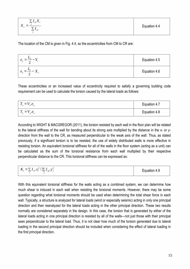
XIX Equation 4.4

The location of the CM is given in Fig. 4.4, so the eccentricities from CM to CR are:

ry YL

e −=2

2 Equation 4.5

rx XL

e −=2

1 Equation 4.6

These eccentricities or an increased value of eccentricity required to satisfy a governing building code requirement can be used to calculate the torsion caused by the lateral loads as follows:

yxx eVT .= Equation 4.7

xyy eVT .= Equation 4.8

According to WIGHT & MACGREGOR (2011), the torsion resisted by each wall in the floor plan will be related to the lateral stiffness of the wall for bending about its strong axis multiplied by the distance in the x- or y-direction from the wall to the CR, as measured perpendicular to the weak axis of the wall. Thus, as stated previously, if a significant torsion is to be resisted, the use of widely distributed walls is more effective in resisting torsion. An equivalent torsional stiffness for all of the walls in the floor system (acting as a unit) can be calculated as the sum of the torsional resistance from each wall multiplied by their respective perpendicular distance to the CR. This torsional stiffness can be expressed as:

∑∑ +=j

jyji

ixit yIxIK 22 .. Equation 4.9

With this equivalent torsional stiffness for the walls acting as a combined system, we can determine how much shear is induced in each wall when resisting the torsional moments. However, there may be some question regarding what torsional moments should be used when determining the total shear force in each wall. Typically, a structure is analyzed for lateral loads (wind or especially seismic) acting in only one principal direction and then reanalyzed for the lateral loads acting in the other principal direction. These two results normally are considered separately in the design. In this case, the torsion that is generated by either of the lateral loads acting in one principal direction is resisted by all of the walls—not just those with their principal axes perpendicular to the lateral load. Thus, it is not clear how much of the torsion generated due to lateral loading in the second principal direction should be included when considering the effect of lateral loading in the first principal direction.

16

4.2 Analysis of Shear-Wall-Frame Buildings

As mentioned before, a simple frame analysis can be conducted in order to evaluate the distribution of lateral load between frames (columns and beams) and walls. Fig. 4.5 presents an example of analytical model. The frame members in the model represent the sums of the stiffnesses of the columns and beams in the building in the bays parallel to the plane of the wall. Similarly, the wall in the model represents the sum of the walls in the structure. The wall and frame are connected by axially stiff link beams at every floor. The link beams in the model shown may or may not be hinged. In computing internal forces and moments due to the factored loads, the flexural stiffnesses, EI, from ACI Code Section 10.10.4.1 may be used. The model in Fig. 4.5 may be acceptable for buildings that are symmetrical in plan and have rigid floor diaphragms. A three-dimensional model is required for an unsymmetrical building, and where a designer wants to account for diaphragm flexibility.

Figure 4.5 - Analytical model of a shear wall-frame building


According to WIGHT & MACGREGOR (2011), the lateral-force analysis of shear-wall–frame buildings must account for the different deformed shapes of the frame and the wall. Due to the incompatibility of the deflected shapes of the wall and the frame, the fractions of the total lateral load resisted by the wall and frame differ from story to story. Near the top of the building, the lateral deflection of the wall in a given story tends to be larger than that of the frame in the same story and the frame pushes back on the wall. This alters the forces acting on the frame in these stories. At some floors the forces change direction, as shown schematically by the range of possible moment diagrams in the wall as shown in Fig. 4.6. As a result, the

frame resists a larger fraction of the lateral loads in the upper stories than it does in the lower stories.

The relative portions of the lateral loads resisted by the walls and frames in a "shear wall–frame building" can be estimated by considering the wall and the frame as two vertical cantilevers, fixed at the bottom and

17

connected via a single extensionally rigid link beam joining the wall and frame at the top, as shown in Fig. 4.6 (a). If the frame is so stiff that it prevents horizontal deflection of the top of the wall, the reaction of the loaded frame at the top of the wall is (3/8.w.hw) where w is the lateral load per foot of height and hw is the height of the wall. This is equivalent to the reaction at the pinned end of a uniformly loaded beam having a constant EI that is fixed at one end and pinned at the other. As the lateral stiffness of the frame decreases relative to the lateral stiffness of the wall, the reaction at the top of the wall decreases, approaching zero for a very flexible frame combined with a stiff wall. As a result, the shear-force and bending-moment diagrams for the wall can vary between the approximate limits shown in Fig. 4.6 (b) and (c). The sum of the shear forces in the frame

and the wall in a given story must equal the shear due to the applied loads.

Figure 4.6 - Effect of frame stiffness on shear and moment in the shear wall.


According to WIGHT & MACGREGOR (2011), two or more shear walls in the same plane (or two wall assemblies) are sometimes connected at floor levels by coupling beams, so that the walls act as a unit when resisting lateral loads, as shown in Fig. 4.7. The discussion will be limited to the case of two walls separated by a single vertical line of openings, which are spanned by reinforced concrete coupling beams. However, walls with more than two lines of openings, are handled similarly to what is discussed for two coupled walls. Other coupled wall systems may need special attention, especially if the widths and heights of the line of

openings are irregular.

18

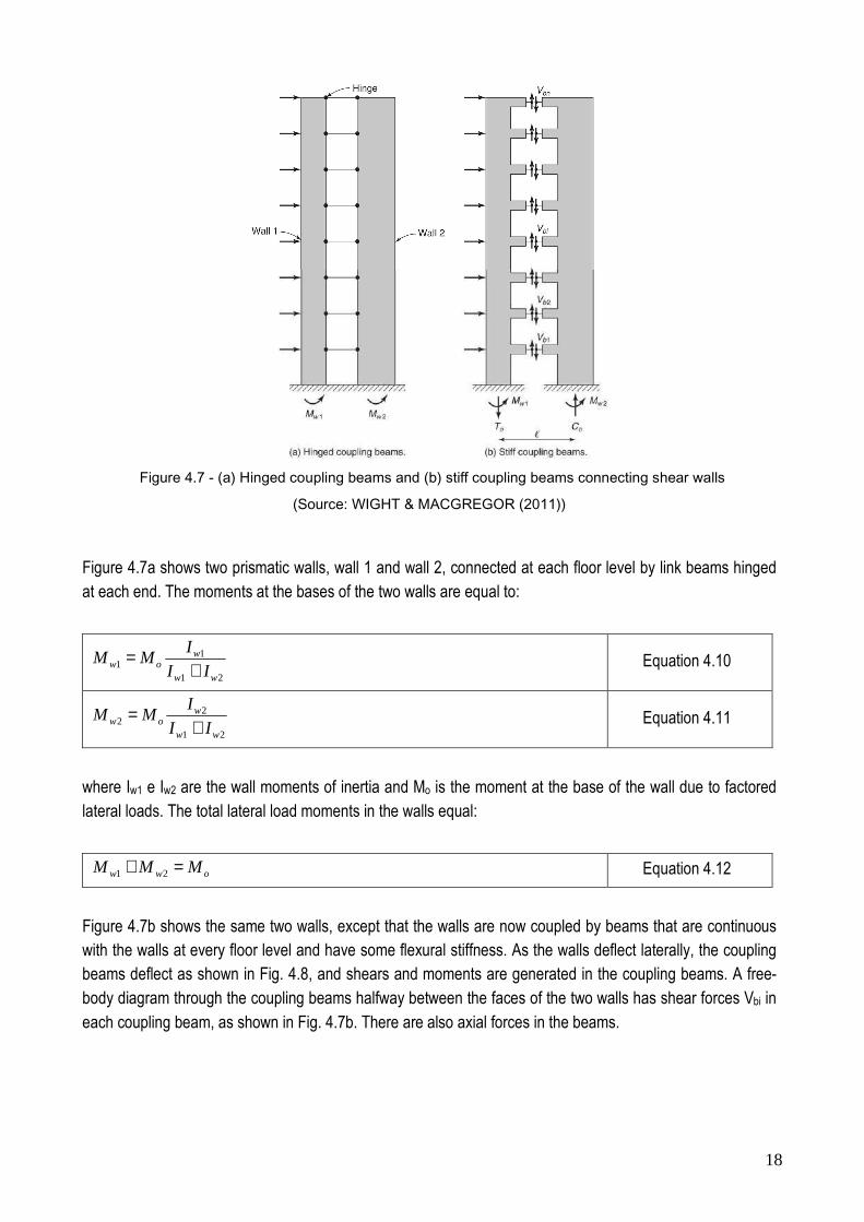
Figure 4.7 - (a) Hinged coupling beams and (b) stiff coupling beams connecting shear walls


Figure 4.7a shows two prismatic walls, wall 1 and wall 2, connected at each floor level by link beams hinged at each end. The moments at the bases of the two walls are equal to:

21

11

ww

wow II

IMM

+= Equation 4.10

21

22

ww

wow II

IMM

+= Equation 4.11

where Iw1 e Iw2 are the wall moments of inertia and Mo is the moment at the base of the wall due to factored lateral loads. The total lateral load moments in the walls equal:

oww MMM =+ 21 Equation 4.12

Figure 4.7b shows the same two walls, except that the walls are now coupled by beams that are continuous with the walls at every floor level and have some flexural stiffness. As the walls deflect laterally, the coupling beams deflect as shown in Fig. 4.8, and shears and moments are generated in the coupling beams. A free-body diagram through the coupling beams halfway between the faces of the two walls has shear forces Vbi in

each coupling beam, as shown in Fig. 4.7b. There are also axial forces in the beams.

19

Figure 4.8 - Effect of shear wall deflections on the forces in a coupling beam


For equilibrium of vertical forces, an axial tension To, must be added to the axial forces in the walls at the centroid of the bottom of wall 1 and an axial compression Co, at the centroid of the bottom of wall 2, where

∑ ===

n

iobio CVT

1 Equation 4.13

Taking the distance between the lines of action of the forces To and Co as l , the total moment at the base of the coupled wall system is:

lTMMM owwo .21 ++= Equation 4.14

WIGHT & MACGREGOR (2011) states that when the coupled wall deflects, the axes of both parts of the wall

at A and A' deflect laterally and rotate through an angle θ, as shown in Fig. 4.8. This results in shearing

deflections of the coupling beams that join the two walls. Localized cracking of the beam-to-wall joint reduces the angle the coupling beam must go through where it is attached to the wall. It is customary to assume the effect of these localized deflections and reduced stiffness of the coupling beam can be represented by moving the assumed connection point in from the face of the wall by approximately hb/2 where hb is the height of the coupling beam. Thus, one may assume the walls are joined by coupling beams spanning from B to B'.

The downward deflection of point B is:

θtan.22

−=∆ bwB

hb Equation 4.15

The moments and axial forces in the two wall segments in Fig. 4.8 must be in equilibrium with the axial forces, shears, and moments in the entire coupled wall system. The signs of the moments and shears may

change over the height of the building.

20

According to WIGHT & MACGREGOR (2011), the beam slenderness (hb/lb) is used as a measure of the stiffness of the coupling beams. A coupling beam with (hb/lb) equal to zero has no flexural stiffness, and as a result, the wall moments are divided in proportion to the ratio of the wall stiffnesses. As the flexural stiffness of the coupling beams increases, the shears in them increase. As a result, the fraction of the overturning moment resisted by the axial force couple To.l increases asymptotically. A major effect of the coupling beams is to reduce the moments Mw1 and Mw2 at the bases of the two walls. This makes it easier to transmit the wall reactions to the foundation. The coupling beams also act to reduce the lateral deflections. If the beams are perfectly rigid, the two walls act as one wall.

In a frame analysis to determine factored moments for design, the member stiffnesses may be based on ACI Code Section 10.10.4.1. The coupling beams are joined to hypothetical members with high values of the moment of inertia, I, between the face of the wall and the centerline of the wall, as shown by the dark shaded regions in Fig. 4.8. Short, deep coupling beams develop both flexural and shear deflections. The shear

deflections can be included by replacing the Ib of the coupling beam between the walls with:

2

8.21

+

=

b

b

beff

l

h

II

Equation 4.16

According to WIGHT & MACGREGOR (2011), this equation comes from adding the moment deflections and shear deflections of the beam, where hb and lb are the depth and the span of the coupling beam from face to face of the walls (adjusted span). The second term in the denominator accounts for the shear deflections of the beam. Floor slabs may serve as soft coupling beams. Their stiffness can be based on a slab with a width perpendicular to the wall equal to the wall thickness plus half of the width of the opening, lb/2, between the walls, added on each side of the opening. In tests of shear walls coupled by slabs, the specimens failed by punching-shear failures in the slab around the ends of the walls. Under cyclic loads, the stiffness of slabs

serving as coupling beams decreased rapidly.

Figure 4.9a, b, and c shows the distributions of moments in the walls, the axial force couple, and the shears in the coupling beams for a typical coupled wall, where Iw1 = Iw2. Typically, the maximum shear in the coupling beams occurs at about one-third of the height above the base. The sawtooth shape of Fig. 4.9a results from

the end moments in the coupling beams.

Figure 4.9 - Typical distribution of (a) wall moments, (b) axial-force couple, and (c) shear in the coupling

beams (Source: WIGHT & MACGREGOR (2011))

21

5. DESIGN OF COUPLING BEAMS

5.1 Equilibrium Relationships

It is well know that lateral forces acting on shear walls will generate opposite rotations at the ends of the beam, causing internal forces at both ends of the coupling beams as illustrated in Figure 5.1. Therefore, coupling beams deform in double curvature. Based on Fig. X, the internal forces for a typical coupling beam

can be deducted as follows:

Figure 5.1 - Internal forces acting at the end of coupling beams

(Source: IHTIYAR (2006))

0..2 =∑ −= cbb lVMM Equation 5.1

al

V

M c

b

b ==2

Equation 5.2

hV

M

h

l

b

bc =2

Equation 5.3

Where

b = beam width;

h = beam height;

lc = clear span of the beam;

a = shear span of the beam.

22

According to IHTIYAR (2006), geometry of coupling beams has a significant effect on their behavior. Moment to shear ratio, defined as shear span ‘a’, is equal to half of the clear span of the beam. Experiments show that, ductility and deformability increases with increasing span length. Increase in span length leads to system controlled by flexure. Reinforced concrete elements controlled by flexure are known to have higher ductility than those controlled by shear. Correspondingly, constructing a deeper and shorter element can lead to shear failure mechanisms. Hence, ratio of shear span to beam depth (a/h) which is defined as the aspect ratio, is an

important geometric parameter for coupling beams.

FEMA 356 (2000) recognizes that “coupled walls are generally much stiffer and stronger than they would be if they acted independently”. This connection between piers increases the moment resisting capacity of the overall system under lateral loading. According to IHTIYAR (2006), the main function of coupling beams is to create a couple at the base of the wall system so that the total moment capacity of the system is increased. End shears at coupling beams at each floor generate axial compression and tensions force in the walls and

the additional moment capacity is simply force times L where L is the lever arm between piers.

JANG & HONG (2004) states that the primary purpose of beams between coupled walls during earthquake actions is the transfer of shear from one wall to the other. In considering the behavior of coupling beams it should be appreciated that during an earthquake significantly larger inelastic excursions can occur in such beams than in the walls that are coupled. During one earthquake, larger numbers of shear reversals can be expected in the beams than in the walls

5.2 Failure Modes

According to PAULAY (1970), the shear in uncracked concrete members is seldom a problem and the traditional concept of principal stresses appears to predict satisfactorily the tensile stresses which are responsible for the initiation of cracking. In beams of normal proportions flexure is the primary cause of cracking and when shear is present, these cracks may incline. Once substantial diagonal cracking has developed, the concept of shear stress must be abandoned. Stress equations are interpreted as giving only an index of shear intensity for an area of a beam where most of a shearing force is being resisted. After cracking various mechanisms may be available which are capable of transferring shear. Whether one allows

for them or not in our strength computation, the existence of such mechanisms must be recognised.

PAULAY (1970) states that across a potential failure section, such as an extended diagonal crack, the shear force can be transmitted in three ways. A part of the transverse force is transferred by shearing stresses, in the compression zone and the remainder by means of aggregate interlock action along the crack and dowel forces across the flexural reinforcement. The mathematical models of analytical studies are, with few exceptions, based on the first mode of shear transfer. In most beams, however, aggregate interlock and dowel action accounts for at least 75% of the shear strength. These actions, which will always be generated

when shear displacements along cracks occur, must also be present in shear walls.

23

PAULAY (1970) describes that when the widening of diagonal cracks is not restricted, as is the case of unreinforced webs of slender beams, it is generally found that the ultimate shear strength is not much in excess of that load which caused diagonal cracking. On the other hand, for short beams, with a shear span to depth ratio of less than 2, considerable shear nay be carried in excess of that causing cracking. Diagonal compression between load points, generally termed arch action, accounts for this. Adequate flexural reinforcement and its full anchorage are prerequisites of arch action. This mode of load transfer is more easily achieved in laboratory beams than in frame components because the load and reactions are generally applied to the top and bottom faces of a test specimen. When the shear is introduced by means of secondary

members the favorable conditions for arch action do not exist.

Theoretical considerations and observations of earthquake damage indicate that the spandrel beams, coupling solid shear walls, are the first ones to be damaged in a well designed structure (PAULAY (1970)).

JANG & HONG (2004) state that the beams of a coupled walls are subjected to large cyclic shear deformations during an earthquake. Hence, one of the most critical problems of these structures concerns the brittle failure of the low slenderness coupling beams. If this failure is avoided, a large fraction of the input seismic energy dissipated by these elements that are distributed throughout these walls. Consequently, building safety will be improved. In this way, two possible failure mechanisms are recognized: flexure failure or shear failure (diagonal tension failure or sliding shear failure).

According to FEMA 306 (2000), flexural failure is characterized as a high ductile behavior mode and in order to obtain flexural behavior, coupling beams should be designed so that (a) diagonal tension and shear sliding failures are avoided and (b) lap splices should be designed properly to prevent splice slip. Flexure failure is characterized by flexural cracks and spalling of concrete during failure. Figure 5.2 shows that flexure cracks are more concentrated at the extreme fibers of the hinging zone. Shear cracks can also be present but crack

width must be less than tenths of an inch (FEMA 306).

Figure 5.2 - Crack pattern of flexurally failed beam


FEMA 306 (1999) recognizes that diagonal tension failure typically occurs in beams having inadequate stirrup reinforcement. Shear forces on a coupling beam generate diagonal cracks from corner to corner of beams and try to split the beam into two triangular sections as seen in Figure 5.3 (JANG & HONG (2004)). Transverse reinforcement acts to hold these pieces together and failure is controlled by yielding of the transverse reinforcement. According to IHTIYAR (2006), diagonal compressive stress might also result in web crushing but this is not commonly seen in coupling beam specimens as axial load is very small and typically

neglected in design.

24

Figure 5.3 - Diagonal tension failure

(Source: JANG & HONG (2004))

According to IHTIYAR (2006), sliding shear failure is common for coupling beams that have a short aspect ratio. Figure 5.4 shows the crack pattern of a sliding failure. Bending moments create vertical flexural cracks at the end zone of the beam. If the beam has sufficient transverse reinforcement to prevent diagonal tension failure, these flexural cracks propagate as loading increases. An almost vertical sliding plane forms near the beam ends at large amplitudes of displacement. Due to concrete deterioration at those regions, shear forces are transferred by only longitudinal reinforcement. However, as concrete deterioration is intensified, longitudinal reinforcement yields and bond strength between steel and concrete decreases, resulting in

strength degradation of the beam.

Figure 5.4 - Crack pattern of shear sliding failure


According to JANG & HONG (2004), the performance-based design philosophy of ductile coupled wall systems allows the coupling beams to form plastic hinges adjacent to beam-wall connections. To carry out this design philosophy, the shear strength of the coupling beams should be greater than flexural yielding force at the ultimate deformation state. After flexural yielding, plastic hinges developed near both ends of the beam, followed by yielding of the shear reinforcement and crushing of the diagonal compressive concrete strut in the plastic hinge region, which led to a sudden failure of the beam.

25

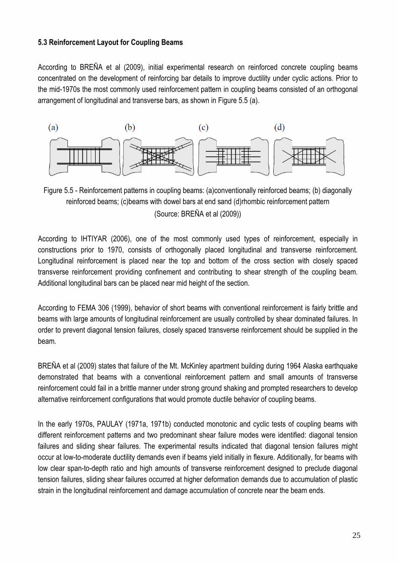
5.3 Reinforcement Layout for Coupling Beams

According to BREÑA et al (2009), initial experimental research on reinforced concrete coupling beams concentrated on the development of reinforcing bar details to improve ductility under cyclic actions. Prior to the mid-1970s the most commonly used reinforcement pattern in coupling beams consisted of an orthogonal arrangement of longitudinal and transverse bars, as shown in Figure 5.5 (a).

Figure 5.5 - Reinforcement patterns in coupling beams: (a)conventionally reinforced beams; (b) diagonally

reinforced beams; (c)beams with dowel bars at end sand (d)rhombic reinforcement pattern

(Source: BREÑA et al (2009))

According to IHTIYAR (2006), one of the most commonly used types of reinforcement, especially in constructions prior to 1970, consists of orthogonally placed longitudinal and transverse reinforcement. Longitudinal reinforcement is placed near the top and bottom of the cross section with closely spaced transverse reinforcement providing confinement and contributing to shear strength of the coupling beam.

Additional longitudinal bars can be placed near mid height of the section.

According to FEMA 306 (1999), behavior of short beams with conventional reinforcement is fairly brittle and beams with large amounts of longitudinal reinforcement are usually controlled by shear dominated failures. In order to prevent diagonal tension failures, closely spaced transverse reinforcement should be supplied in the

beam.

BREÑA et al (2009) states that failure of the Mt. McKinley apartment building during 1964 Alaska earthquake demonstrated that beams with a conventional reinforcement pattern and small amounts of transverse reinforcement could fail in a brittle manner under strong ground shaking and prompted researchers to develop

alternative reinforcement configurations that would promote ductile behavior of coupling beams.

In the early 1970s, PAULAY (1971a, 1971b) conducted monotonic and cyclic tests of coupling beams with different reinforcement patterns and two predominant shear failure modes were identified: diagonal tension failures and sliding shear failures. The experimental results indicated that diagonal tension failures might occur at low-to-moderate ductility demands even if beams yield initially in flexure. Additionally, for beams with low clear span-to-depth ratio and high amounts of transverse reinforcement designed to preclude diagonal tension failures, sliding shear failures occurred at higher deformation demands due to accumulation of plastic strain in the longitudinal reinforcement and damage accumulation of concrete near the beam ends.

26

To promote ductility, PAULAY (1971b) and PAULAY & BINNEY (1974) proposed a reinforcement pattern consisting of sets of diagonally placed bars extending from corner to corner of coupling beams (Fig. 5.5b) following observed cracking patterns in laboratory tests and to avoid premature failures associated with low ductilities due to crack widening at beam ends To avoid buckling, diagonal bars are typically laterally supported using closely spaced hoops because they are expected to undergo large inelastic load reversals.

PAULAY & SANTHAKUMAR (1976) compared the effect of coupling beam reinforcement pattern on lateral-load response of coupled wall systems by testing one-quarter scale coupled wall models with conventionally reinforced beams or diagonally reinforced beams (see Fig. 5.5(b)). Their results indicated that sliding shear failure could occur at the end of conventionally reinforced coupling beams after several cycles of shear reversal. In contrast, beams with diagonal reinforcing bars exhibited stable response without strength or stiffness degradation at large displacements.

According to BREÑA et al (2009), current and past codes (UBC 1997; IBC 2009; ACI 318-08) promote use of diagonal bars in coupling beams with low aspect ratios and high shear stresses. Diagonally reinforced beams, however, have proved difficult to build in practice due to reinforcement congestion, horizontal and vertical bar interference, and the need for confinement reinforcement. With the goal of simplifying construction without sacrificing ductile response, several investigators have proposed alternate reinforcement configurations that

would improve the performance of coupling beams under large load reversals.

Experiments show that specimens with heavy transverse and longitudinal reinforcement may fail due to sliding shear at the end zones after a number of load applications. To avoid shear sliding failures, TASSIOS et al (1996) have proposed the utilization of short or long dowels at the end zones as seen in Figure 5.7c. These dowels contribute to shear sliding capacity until bond between dowels and concrete is lost due to cracking at hinging regions. Hence, rapid shear strength degradation is inevitable and brittle failure was

ultimately observed.

Some additional layout configurations have been proposed for coupling beams, as for example, the Rhombic layout introduced by TEGOS & PENELIS (1998) presented in Figure 5.7.d. The idea is to create a rhombic truss system which is the most effective solution to prevent shear failure for low slenderness elements. Although results from tests have been very successful, the constructability of the reinforcement pattern is not as practical as the other reinforcement types. Hybrid coupling beams by using structural steel elements embedded within the reinforced concrete beam cross section also have been proposed (HARRIES et al

(1997)).

27

6. EXPERIMENTAL RESULTS: AMHERST COUPLING BEAMS

6.1 General Description of the Experimental Research Four coupling beam specimens were tested by IHTIYAR (2006) with the primary intent to investigate effects of reinforcing characteristics on the observed failure mode. Specimens were designed using a concrete mix with a nominal compressive strength of 30 MPa. Nominal yield strength of the longitudinal and transverse reinforcement was 410 MPa, except for specimen CB-2 that had transverse reinforcement consisting of deformed wire with a nominal yield strength of 580 MPa. Figure 6.1 illustrates the geometry and reinforcement patterns of the four specimens tested in this research. Figure 6.2 shows the obtained results for the concrete used in the beams and Figure 6.3 shows the strength of the reinforcement.

Figure 6.1 - Specimen geometry, reinforcing details and measured material properties (Source: BREÑA & IHTIYAR (2011)

28

Figure 6.2 - Concrete used in the coupling beams

(Source: BREÑA & IHTIYAR (2011)

Figure 6.3 - Reinforcement used in the coupling beams

(Source: BREÑA & IHTIYAR (2011)

Forces were generated in the coupling beams by applying horizontal forces to two stiff concrete walls constructed on each end of the specimens (see Fig.6.4). Horizontal loading was distributed to the top of the walls using a stiff steel element that imposed equal lateral displacement to both walls. Given the geometry of the test setup, an applied lateral force Q generated shear forces at the ends of the coupling beams equal to Q.hpin/(ln+lw), giving shears of 1,1 and 0,8 times Q for the short (CB-1 and CB-3) and long (CB-2 and CB-4)

specimens, respectively.

Figure 6.4 - Test setup for the Amherst Walls (Source: BREÑA & IHTIYAR (2011))

29

Lateral force was applied cyclically in sets of three cycles at pre-defined amplitudes as shown in Figure 6.5. Applied loading was force-controlled in pre-yield stages and subsequently changed to displacement control at post-yield stages. At loading stages below the estimated yield shear force (Vy), the applied loading amplitudes were 1/3, 2/3, and 3/3 of Vy. The lateral displacement at the top of the walls at Vy was defined as the displacement at yield. Subsequent loading was applied in increments of 0.5 times the yield displacement. Loading was stopped as specimens began to lose strength at higher applied displacements since the primary intent was to determine the stiffness of the loading branch and the factors contributing to coupling beam deformation.

Figure 6.5 - Loading history of the specimens


Figure 6.6 - Cyclic shear force-chord rotation response of the tested coupling beams

(Source: BREÑA & IHTIYAR (2011))

30

The cyclic shear force-chord rotation behavior of the four beams tested in the experimental program are shown in Figure 6.6, from which several response features can be highlighted. Specimens CB-1 and CB-3 (short span) exhibited essentially similar cyclic characteristics. Both specimens reached approximately the same shear force and were able to develop similar chord rotations at yield and peak shear force. The influence of horizontal web reinforcement in CB-3 did not affect the general characteristics of the hysteretic

response significantly, but did increase the measured chord rotation at yield.

The highly contrasting behavior of specimens CB-2 and CB-4, although with the same span to-depth ratio, was primarily caused by the significantly different amounts of transverse reinforcement. Transverse reinforcement in CB-2 was barely sufficient to maintain shear strength after formation of the first diagonal crack and resulted in a brittle failure mode with no yielding of the longitudinal reinforcement. On the other hand, CB-4 had a very ductile response as a result of low flexural strength (Vf) and relatively high shear capacity (Vn). Specimen CB-4 was the only beam that had a higher shear strength than required to develop plastic hinging and spread of plasticity near beam ends. Also, only specimen CB-4 was taken to much higher displacements because it was designed to be flexurally dominated and its shear retention capacity at large displacements (residual strength) was of particular interest. Table 6.1 shows the shear strength of the tested coupling beam specimens.

Table 6.1 - Shear strength of the tested coupling beams

Specimen Vy,test (kN) Vmax,test (kN)

CB-1 414 478

(test halted before failure)

CB-2 226 275

CB-3 409 506

(test halted before failure)

CB-4 142 240

According to BREÑA & IHTIYAR (2011), unlike Specimens CB-1 and CB-3, which exhibited extensive cracking throughout their span, cracking in Specimens CB-2 and CB-4 was concentrated primarily near the beam ends. Observed cracking in these specimens was similar to that observed in the hinging regions of slender beams, although diagonal cracks almost joined near midspan at higher displacement amplitudes in Specimen CB-2, and remained concentrated near the beam ends in Specimen CB-4.

6.2 Behavior of the Specimen CB-1

Figure 6.7(a) through (f) depicts the propagation of cracks of the front side of the beam CB-1 at each load step. Specimen CB-1 was designed to have a shear sliding failure by referring to FEMA 306 (1999) strength equations. During first load step, vertical cracks were formed at both ends of the beam. Corner to corner diagonal crack was first generated at the back side of the beam during load step 3, at the yield displacement δy. Increasing the lateral displacement caused the propagation and widening of the cracks. Flexural cracks around the top pin were also observed at VBeam equals to 364,73 kN but due to low aspect ratio of the beam, shear forces dominate the cracking pattern. At load step 7 (2.5 δy), residual width of vertical cracks reached

31

up to 1,52 mm. Concrete crushing around the corners of the beam also started to occur at this cycle and the

test was ended due to failure of the pier around the top pin.

Figure 6.7 - Cracking pattern of the coupling beam CB-1 at (a) Load step 2 (b) Load step 3 (c)Load step

4 (d) Load step 5 (e) Load step 6 and (f) Load step 7. (Source: IHTIYAR (2006))

According to IHTIYAR (2006)), strain values of the stirrups were minimal during the first two load steps. After the formation of diagonal crack at load step 3, a sudden jump was recorded in stirrup strain readings because shear forces were started to be resisted only by the stirrups. Closely spaced stirrups prevented excessive widening of diagonal cracks on the specimen for the following load steps. At a beam shear force of 414 kN, strain in transverse bars reached up to a value of approximately 0,002 approximately corresponding to yielding of the bar. Like with the stirrups, strain on longitudinal bars saw sudden increase around a shear force of 444 kN and widening of vertical cracks can be the reason for this excessive longitudinal bar

deformation.

According to BREÑA & IHTIYAR (2011), strain gauges on the stirrups were positioned to approximately follow the direction of the anticipated diagonal cracking in the beams (between 40° and 50° from the horizontal), so the point of measurement may have actually ended up at some distance from the actual location of cracks. Nevertheless, strains exceeding the yield value were observed in stirrups in several cases, particularly at locations corresponding to midheight of the beams. Lateral deflection (or drift) at the yielding (δy) was measured to be 1,016 cm and Specimen CB-1 was able to be loaded up to a shear force of approximately 492 kN. Figure 6.8 shows the failure condition of Specimen CB-1 while Figure 6.9 shows the

strains.

32

Figure 6.8 - Failure condition for Specimen CB-1 (Source: IHTIYAR (2006))

Figure 6.9 - Strains obtained for Specimen CB-1


33

6.3 Behavior of the Specimen CB-2 According to IHTIYAR (2006), diagonal tension failure was the predicted failure mode for this specimen (FEMA 306, 1999) because of inadequate transverse reinforcement. Cracking pattern and failure mode of the specimen CB-2 is shown in Figure 6.10. Similar with specimen CB-1, vertical cracks at both beam ends occurred at the first load step. Diagonal cracks were then generated at second load step. Residual widths of the critical diagonal crack were around 0,127 mm. At next load cycle, the crack widths were approximately doubled. Due to inadequate transverse reinforcement content, the specimen had a catastrophic diagonal tension failure at load cycle 4.

Figure 6.10 - Failure condition for Specimen CB-2


The angle of the crack was very close to 45 degrees and there were three stirrups located at the crack zone. Concrete interlock was totally lost and three stirrups were not sufficient to maintain the beam shear force and all of them fractured. After losing these stirrups, shear transfer could not be achieved and sudden strength loss was observed. Yield displacement δy was measured to be 1,09 cm and according to BREÑA & IHTIYAR (2011), longitudinal bar strains in Specimen CB-2 were the lowest registered of the four

specimens tested.

According to BREÑA & IHTIYAR (2011), the widely spaced transverse reinforcement caused shear failure at low displacements, resulting in limited yielding of longitudinal reinforcement. As longitudinal reinforcement yielded, the second stirrups from each end of the beam were crossed by a major diagonal crack, causing strains to increase beyond the yield strain. Because of the low amount of existing transverse reinforcement, stirrups were incapable of carrying the applied shear force, causing the ensuing specimen failure. This limited the amount of plastic deformations that other bar sections could develop. The failure initiated by the yielding of one of the stirrups situated at the end of the beam for a shear force of about 226 kN and the specimen failed after the rupture of the same stirrup at the shear force of 257 kN. For this same load, the yielding of the top reinforcement has started leading the coupling beam to the failure. Figure 6.11 shows the strains for

Specimen CB-2.

34

Figure 6.11 - Strains obtained for Specimen CB-2


35

6.4 Behavior of the Specimen CB-3 According to IHTIYAR (2006), shear sliding failure was the predicted failure mode for this specimen (FEMA 306, 1999). Cracking of specimen CB-3 was very similar with specimen CB-1, i.e, shear cracks dominated the pattern because of low aspect ratio. Vertical cracks at beam ends were seen in the first load step. At second load step, diagonal cracks started to occur having an average residual width of 0,050 mm. When compared with specimen S1, diagonal cracking was more intense probably due to higher shear forces. At the back side of the beam, rather than many small diagonal cracks, one large corner to corner crack was formed with a residual crack width of 0,22 mm (0,635 mm peak width). Application of further load steps caused the propagation of existing cracks and formation of new diagonal cracks. Test was stopped due to bending of the bottom pin support and concrete crushing around it. Vertical cracks had a maximum residual width of 0,40

mm. Figure 6.12 shows the pattern cracking for the specimen CB-3.

Figure 6.12 - Frontside crack pattern of the specimen CB-3 at (a)Load step 2 (b) Load step 3 (c)Load step

4 (d) Load step 5 (e) Concrete Crushing at load step 5 (f)Bending of the bottom pin. (Source: IHTIYAR (2006))

According to BREÑA & IHTIYAR (2011), stirrup strains were lower in Specimen CB-3 than in CB-1, perhaps because of the formation of a more densely distributed crack network resulting from the presence of intermediate longitudinal bars. At load step 2, the strain values suddenly increased due to formation of diagonal cracking. At the peak shear, stirrup readings were around 0.002 which is the yield strain of steel. Failure started with the yielding of the main reinforcement for a shear force of about 409 kN. For a shear force of about 445 kN the stirrups started to yield and failure was finally observed for a shear force of about 506 kN. Fig 6.13 shows the strains for specimen CB-3.

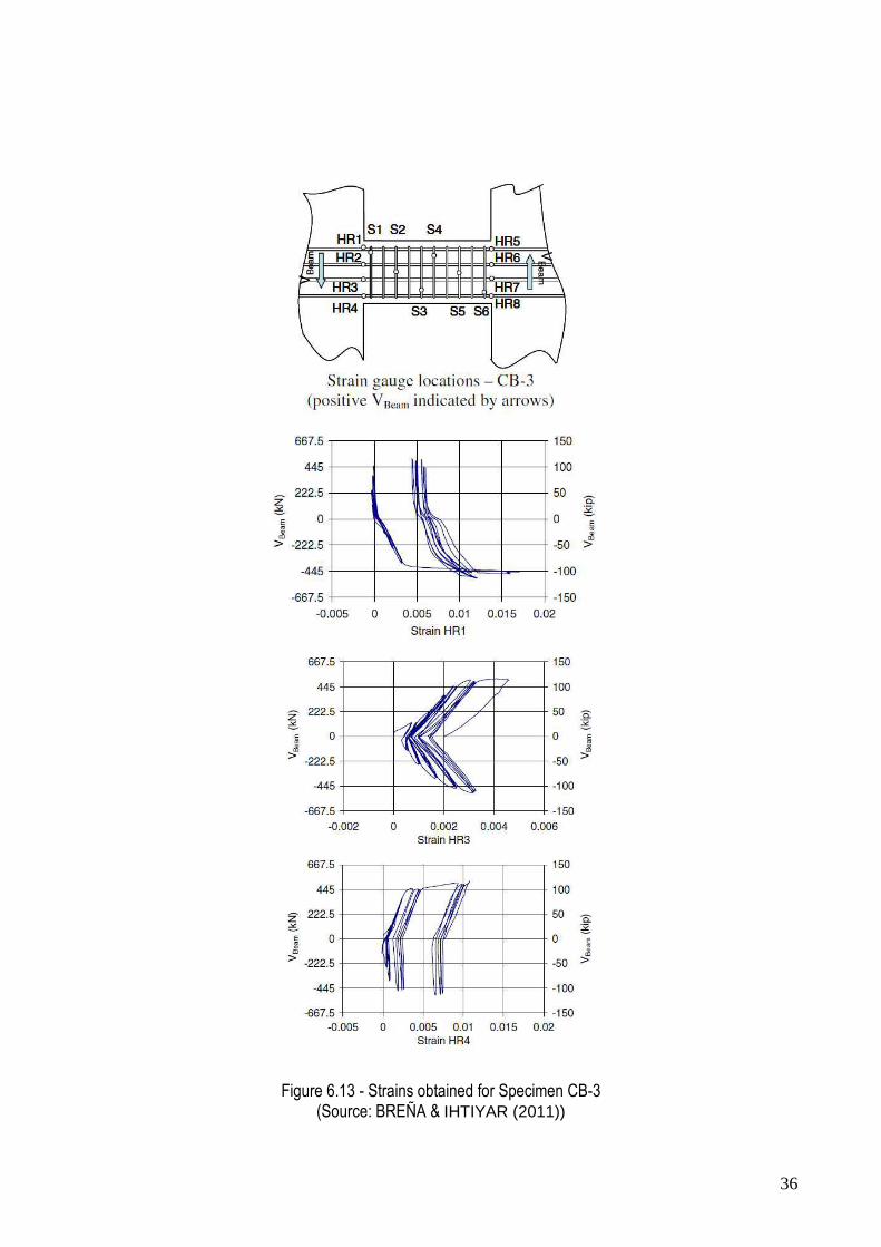
36

Figure 6.13 - Strains obtained for Specimen CB-3 (Source: BREÑA & IHTIYAR (2011))

37

6.5 Behavior of the Specimen CB-4 According to IHTIYAR (2006), Specimen CB-4 was designed to have ductile behavior since diagonal tension failure was prevented by placing closely spaced stirrups. Figure 6.14 shows the cracking pattern of the

Specimen CB-4 for several load steps.

Figure 6.14 - Frontside crack pattern of the coupling beam CB-4 at (a)Load step 1 (b) Load step 2 (c)Load

step 3 (d) Load step 4 (e) Load step 5 (f) Load step 6 (g) Load step 7 (h) Load step 8 (i) Load step 9 (Source: IHTIYAR (2006))

According to IHTIYAR (2006), in addition to vertical cracks, flexural cracks were observed in the second load step. Unlike specimen CB-2, which has the same aspect ratio, diagonal cracks were not formed at early load steps on this specimen because of sufficient transverse reinforcement content. Flexural cracks were mostly located close to beam corners due to larger moment values at the ends. With the propagation of vertical cracks at beam corners, a failure plane started to form at beam ends. Residual width of these cracks was around 0,254 mm at load step 4. Vertical shear plane became more apparent at the following load cycles with residual crack widths reaching up to 1,06 mm. Concrete interlock started to degrade with the widening of vertical cracks. Maximum residual crack was measured to be 3,175 mm at load step 8 after which Specimen

CB-4 started to lose strength.

Figure 6.15(a) shows the close up view of the failure. Concrete interlock was almost lost and shear transfer was accomplished only by horizontal bars, termed as the dowel action. Test was halted due to fracture of the

longitudinal bars as seen in Figure 6.15(b). This type of behavior is an example of shear sliding failure.

38

Figure 6.15 - (a) Shear sliding failure and (b) rupture of the main reinforcement of the Specimen CB-4

(Source: IHTIYAR (2006)) The middle section of the beam did not crack significantly but concrete carried the portion of shear force in that region. The strain readings obtained in the stirrups were smaller than yield strain and there wasn’t any indication of diagonal tension failure. Failure started when both longitudinal bars reached the yield strain of 0.002 at a shear force of around 142 kN. The specimen failed for a shear force of about 240 kN, with longitudinal strains very close to the strain rupture of the bars and very low strains for the stirrups. Figure 6.16

shows the cracking pattern of Specimen CB-4 at failure.

Figure 6.16 - Cracking pattern at failure for Specimen CB-4


According to BREÑA & IHTIYAR (2011), longitudinal bar strains in Specimen CB-4 exhibited significant yielding in a very stable manner because of the large amount of transverse reinforcement contained in this specimen. Except for the strains measured in strain gauge S5, other stirrup strains remained below the yield strain, as shown for S2. Longitudinal bar strains, however, registered values exceeding yielding, with peak measurements of more than 3.5% registered on the left end of the beam (instruments HR1 and HR2 of Fig

6.17).

39

Figure 6.17 - Strains obtained for Specimen CB-4 (Source: BREÑA & IHTIYAR (2011))

40

7. SIMULATIONS OF THE TESTED COUPLING BEAMS

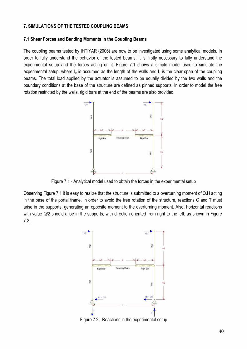
7.1 Shear Forces and Bending Moments in the Coupling Beams The coupling beams tested by IHTIYAR (2006) are now to be investigated using some analytical models. In order to fully understand the behavior of the tested beams, it is firstly necessary to fully understand the experimental setup and the forces acting on it. Figure 7.1 shows a simple model used to simulate the experimental setup, where lw is assumed as the length of the walls and ln is the clear span of the coupling beams. The total load applied by the actuator is assumed to be equally divided by the two walls and the boundary conditions at the base of the structure are defined as pinned supports. In order to model the free rotation restricted by the walls, rigid bars at the end of the beams are also provided.

Figure 7.1 - Analytical model used to obtain the forces in the experimental setup

Observing Figure 7.1 it is easy to realize that the structure is submitted to a overturning moment of Q.H acting in the base of the portal frame. In order to avoid the free rotation of the structure, reactions C and T must arise in the supports, generating an opposite moment to the overturning moment. Also, horizontal reactions with value Q/2 should arise in the supports, with direction oriented from right to the left, as shown in Figure 7.2.

Figure 7.2 - Reactions in the experimental setup

41

In order to obtain the equilibrium of the structure, the overturning moment must be equal the stabilizing moment provided by T or C. In this way, it is easy to prove that C and T need to be equal to Q.H/L. Once the reactions acting in the pinned supports are know, it is possible to fully obtain the shear forces and bending moment acting in the portal frame, as shown in Figure 7.3. Figure 7.3 shows that the bending moments acting in the faces of the walls are defined by (0,25.Q.H.ln)/(0,5.ln+0,5.lw). By another hand, the shear forces acting

in the coupling beams are constant throughout the whole span.

Figure 7.3 - Bending moments and shear forces acting in the experimental setup

Assuming that for specimens CB-1 and CB-3, lw = 0,76 m, ln = 0,51 m, L = 1,27 m and H = 1,40 m, the maximum shear force will be Vmax = 1,1.Q and the maximum bending moment at the face of the wall will be Mmax = 0,281.Q. By another hand, assuming that for specimens CB-2 and CB-4, lw = 0,72 m, ln = 1,02 m, L = 1,74 m and H = 1,40 m, the maximum shear force will be Vmax = 0,8.Q and the maximum bending moment

at the face of the wall will be Mmax = 0,410.Q.

7.2 Chord Rotation in the Coupling Beams In FEMA 356 (2000), beam chord rotation is used as a deformation parameter for coupling beams. Unfortunately, IHTIYAR (2006) revealed that was impossible to measure the beam end rotation with the proposed test setup. Hence, global lateral deformation of the structure was used to derive rotation of the coupling beams using the package software FTOOL.

As recommended by FEMA 356 (2000), a cracked moment of inertia of 0.5 EcIg was defined for the coupling beam and the walls, observing that flexural cracks were also observed in the walls during the tests for all specimens. A rigid bar, with a very large moment of inertia, was defined in the intersection of the coupling beam and the walls and the dead load on the specimens was neglected. A unit displacement, ∆wall was

applied to both walls and the chord rotation of the beam (θBeam) was determined. Figure 7.4 shows the model

constructed in the package software FTOOL.

42

Figure 7.4 - Model used to obtain the chord rotation of the coupling beams

Considering the elastic modulus of the concrete as 5600.(fc)1/2 the following relationships between displacements (mm) and chord rotations (radian) may be obtained for the coupling beams as indicated in Table 7.1, with ∆wall em mm:

Table 7.1 - Chord rotation of coupling beams using FTOOL

Specimen f'c

(MPa)

Cracked elastic modulus (0,5.Ec)

(MPa)

Chord Rotation

(radian)

CB-1 39,1 17508,39 θBeam = (0,000445) ∆wall

CB-2 38,7 17418,61 θBeam = (0,000563) ∆wall

CB-3 31,4 15689,99 θBeam = (0,000445) ∆wall

CB-4 30,6 15488,83 θBeam = (0,000563) ∆wall

Shear stiffness degradation is observed to be significant for coupling beams. In this way, Icr may be estimated by using the relation proposed by Paulay and Priestley (1992), where h is the height of the beam and lc the

clear span of the coupling beam:

+

=2

31

.2,0

c

gcr

l

h

II

Equation 7.1

Equation 7.1 can be used to better estimate yield rotation for previously tested specimens, i.e, the above equation may give a estimation better than 0,5 EcIg proposed by FEMA 356 (2000). By using Equation 7.1, flexural stiffness for the coupling beams of specimens CB-1 and CB-3 is calculated as 0,075.EcIg and for the coupling beams of the specimens CB-2 and CB-4 the flexural stiffness is calculated as 0,141.EcIg. In this way, defining the calculated flexural stiffness just for the coupling beams (not for the walls), the following chord

rotations can be found (rotations in radians and displacements in mm): θBeam = (0,000624).∆wall (for

Specimens CB-1 e CB-3) and θBeam = (0,0006175).∆wall (for Specimens CB-2 and CB-4) with ∆wall em mm.

43

7.3 Predictions Using Analytical Models 7.3.1 ACI-318, ASCE/SEI 41-06, FEMA 356 and FEMA 306 The coupling beam strength in ASCE/SEI 41-06 (ASCE 2006) and FEMA 356 is calculated in accordance with techniques in the American Concrete Institute (ACI) Building Code (ACI 2008), employing actual (or expected) material strengths and a strength reduction factor (or partial safety factors) equal to 1.0 in all equations. Basically, nominal flexural strength (Mn) is determined from basic principles accounting for

contribution of multiple longitudinal reinforcement layers, if present.

Bending moments can be related to beam shear force from equilibrium considerations by assuming an effective length of the beams. The shear force in the beams will then depend on the plastified length at the beam ends. For little yield spreading in the longitudinal reinforcement (such as for the condition at yield or brittle shear failure modes), end moments may be assumed acting at the beam-wall connection, but for conditions where significant yield penetration has occurred (stable plastic hinging at anticipated flexural strength) moments are assumed to act at the end of the plastified region. Thus, shear forces corresponding to

these two conditions can be calculated using Eqs. (7.2) and (7.3), respectively:

n

nflex l

MV

.2= (Equation 7.2)

pn

nflex ll

MV

−= .2

(Equation 7.3)

In the last equations, ln is the beam clear span, and lp is an assumed plastic hinge length. The recommended plastic hinge length in ASCE/SEI 41-06 is the beam flexural depth divided by 2. In short deep members such as coupling beams, the shear force required to develop hinging may be quite large as the difference between

the clear span and plastic hinge length can be very small (it approaches zero when ln = h).

Coupling beam shear strength (diagonal tension) is calculated using (ACI 318-08 Eq. 21-7), which for normalweight concrete is:

)( 'ytvcccvn ffAV ρα += (Equation 7.4)

In the last equation, where αc is equal to 3 for a clear span to depth ratio ln/h < 1,5, or 2 for ln/h > 2 (linear interpolation is conducted for values in between); ρv = Av/(bws) is the transverse reinforcement ratio; Acv is the cross sectional area of the beam parallel to the application of shear force; bw is the beam web width; fyt is the expected yield stress of transverse reinforcement at a spacing s.

According to BREÑA et all (2009), one of the limitations of Eq. 7.4 is that it does not recognize the shear strength degradation that occurs with beam cycling, nor other shear failure modes that can occur and that have been documented for coupling beams (e.g. sliding shear). This could be due to strength degradation or sliding shear modes typically occurring at higher deformation demands. Other available documents provide

44

more detailed procedures to estimate shear strength as a function of displacement ductility (FEMA 306, for

example).

Recognizing two potential types of shear failure in coupling beams, FEMA 306 (ATC 1999) provides separate procedures to determine nominal shear strength associated with diagonal tension or sliding shear failures based on the ductility capacity. Maximum displacement ductility is defined in terms of chord rotation, θ, as the

ratio between rotations at ultimate and yield (µ∆ = θu / θy). In this way, ductility capacity is classified in FEMA

306 as low if µ∆ is less than two, moderate if it is between two and five, and high if µ∆ is greater than 5.

Nominal diagonal tension strength of coupling beams (Vn-dt) is calculated using the following equation

(notation is slightly modified from that used in FEMA 306 for consistency in this report):

)'dwytvwcrcscdtn hbfdbfkVVV ραβ +=+=− (Equation 7.5)

FEMA 306 allows estimating the effective depth (d) as 0,8h to account for multiple reinforcement layers. The first and second terms correspond to the concrete (Vc) and transverse reinforcement (Vs) contribution to shear strength, respectively. The contribution of transverse reinforcement to shear strength of coupling beams is

calculated by estimating the horizontal length, hd = (h - c).cotφ, over which transverse reinforcement

contributes to shear strength, where c = neutral axis depth. The neutral axis depth may be estimated using

the recommendation of HSU & MO (2010) based on the transformed cross-section, as shown in Figure 7.7.

Figure 7.7 - Neutral axis of doubly reinforced concrete beams (HSU & MO (2010))

Assuming n = Es,bottom/Ec , m = Es,top/Ec, Ec = 5600 (fc')1/2, ρ = As,bottom/Ac, ρ' = As,top/Ac, the following equations

can provide the neutral axis (c) for a doubly reinforced beam:

ρρβ

n

mc

'

= (Equation 7.6)

)1()'

.1.(2)1.()( 22ccc n

d

dnnk βρβρβρ +−+++= (Equation 7.7)

45

Diagonal cracks are assumed to form at an angle φ = 35° from the horizontal, unless a steeper crack is expected to form from corner to corner of the beam. The constant, krc, is a function of ductility and has a value

of 3,5 at low displacement ductility (µ∆ < 2), and decreases linearly to 0,6 at high displacement ductility (µ∆ >

5). The effects of shear span and the dowel action of longitudinal reinforcement on shear strength are

accounted through constants α = 3 - M/(0,8.h.V) and β = 0,5 + 20ρg, where ρg = total area of longitudinal

reinforcement divided by the gross cross-sectional area. The constant α, is bound between 1,0 and 1,5, and

β may not exceed 1,0. Once M/V is calculated to be ln/2 in coupling beams, α can be rewritten as α = 3 -

0,625.ln/h.

The sliding shear strength, Vns, of coupling beams can be estimated from FEMA 306 (ATC 1999), as follows,

observing that for coupling beams, the constant C is equal to 3,0 or 1,2 for moderate (2 < µ∆ < 5) or high

ductility (µ∆ > 5) demands, respectively.

dbfh

lCV wc

nns

'

= (Equation 7.8)

Taking into account the presented equations, the analytical failure loads may be estimated for the tested coupling beams. For the specimen CB-1, the following parameters are assumed:

bw = 25 cm = 10"

h = 38 cm = 15"

d = 34 cm = 13,4"

ln = 51cm = 20"

Asl = 3#5 = 6,0 cm2 = 0,93 in2

fyl = 517 MPa = 75 ksi = 75000 psi

Ast = #3 c/ 5 cm = #3 c/2"

fyt = 524 MPa = 76 ksi = 76000 psi

fc' = 39,10 MPa = 5668 psi

My = 95,90 kN.m (see RESPONSE 2000 results ahead)

Mu = 113,80 kN.m (see RESPONSE 2000 results ahead)

The flexural strength of the specimen, according to ASCE/SEI 41-06 will be:

kNl

MV

n

yy 07,376

51,090,95.2.2

===

kNl

MV

n

uu 27,446

51,080,113.2.2 ===

46

The shear strength (diagonal tension), according to ACI-318 and ASCE/SEI 41-06 will be:

ln/h = 0,51/0,38 = 1,34 → αc = 3

Acv = bw.h = 10".15" = 150 in2

ρv = Av/(bw.s) = 2.0,11/(10".2") = 0,011

)( 'ytvcccvn ffAV ρα +=

kNkipspoundsVn 47,70827,15975,159278)76000.011,056683.(150 ===+=

The shear strength (diagonal tension), according to FEMA 306 will be:

Ec = 5600.(fc')1/2 = 5600.(39,1)1/2 = 35016,79 MPa

n = Es/Ec = 200000/35016,79 = 5,71 = m

ρ = ρ' = As/Ac = 3.2/(25.38) = 0,0063

βc = mρ'/nρ = 1,0

)1()'

.1.(2)1.()( 22ccc n

d

dnnk βρβρβρ +−+++=

22,0)11.(0063,0.71,5)344

.11.(0063,0.71,5.2)11.()0063.71,5( 22 =+−+++=k

c = k.d = 0,22.13,4" = 2,948" hd = (h - c).cotgφ = (15"-2,948").cotg 35o = 17,21"

α = 3 - (0,625.ln/h) = 3 - (0,625.20"/15") = 2,16→ α=1,5 once 1,0 < α < 1,5 ρg = Asl/Ac = (6.0,31)/(10".15")=0,0124

β = 0,5 + 20.ρg = 0,5 + 20.0,0124 = 0,748 < 1,0 (ok!)

For µ∆ < 2 → krc = 3,5

dwytvwcrcscdtn hbfdbfkVVV ραβ +=+=−'

kNkipspoundsV dtn 54,81657,18311,18357621,17.10.76000.011,04,13.10.56685,3.748,0.5,1 ===+=−

For µ∆ > 5 → krc = 0,6



The sliding shear strength, according to FEMA 306 will be:

For 2 < µ∆ < 5 → C = 3,0

dbfh

lCV wc

nns

'

=

kNkipspoundsVns 49,17935,4036,403534,13.10.5668"15"20

.0,3 ===

=

47

For µ∆ > 5 → C = 1,2

dbfh

lCV wc

nns

'

=


.2,1 ===

=

Figure 7.8 presents all the predictions using the analytical equations. As one can see, specimen CB-1 is dominated by flexure and after the yielding of the main reinforcement, shear sliding failure will dominate the

final behavior.

Figure 7.8 - Expected load path using analytical expressions for specimen CB-1

For the specimen CB-2, the following parameters are assumed:

bw = 25 cm = 10"

h = 38 cm = 15"

d = 34 cm = 13,4"

ln = 102 cm = 40"

Asl = 3#6 = 8,52 cm2 = 1,32 in2

fyl = 445 MPa = 64,5 ksi = 64500 psi

Ast = D4 c/ 16 cm = D4 c/6,3"

fyt = 606 MPa = 87,8 ksi = 87800 psi

fc' = 38,70 MPa = 5616 psi



48


kNl

MV

n

yy 66,226

02,160,115.2.2

===

kNl

MV

n

uu 43,298

02,120,152.2.2 ===


ln/h = 1,02/0,38 = 2,68 → αc = 2

Acv = bw.h = 10".15" = 150 in2

ρv = Av/(bw.s) = 2.0,04/(10".6,3") = 0,0012


kNkipspoundsVn 29,17028,3899,38285)87800.0012,056162.(150 ===+=


Ec = 5600.(fc')1/2 = 5600.(38,70)1/2 = 34837,22 MPa

n = Es/Ec = 200000/34837,22 = 5,74 = m

ρ = ρ' = As/Ac = 3.2,84/(25.38) = 0,0089

βc = mρ'/nρ = 1,0

)1()'

.1.(2)1.()( 22ccc n

d


25,0)11.(0089,0.74,5)344

.11.(0089,0.74,5.2)11.()0089.74,5( 22 =+−+++=k


α = 3 - (0,625.ln/h) = 3 - (0,625.40"/15") = 1,33 → α=1,33 once 1,0 < α < 1,5 ρg = Asl/Ac = (6.0,44)/(10".15")=0,0176

β = 0,5 + 20.ρg = 0,5 + 20.0,0176 = 0,852 < 1,0 (ok!)

For µ∆ < 2 → krc = 3,5



For µ∆ > 5 → krc = 0,6



49


For 2 < µ∆ < 5 → C = 3,0

dbfh

lCV wc

nns

'

=


.0,3 ===

=

For µ∆ > 5 → C = 1,2

dbfh

lCV wc

nns

'

=


.2,1 ===

=

Figure 7.9 presents all the predictions using the analytical equations. As one can see, specimen CB-2 is dominated by shear (diagonal tension) and the main reinforcement is not supposed to present yielding.



bw = 25 cm = 10"

h = 38 cm = 15"

d = 34 cm = 13,4"

ln = 51cm = 20"

Asl = 3#5 = 6,0 cm2 = 0,93 in2

fyl = 517 MPa = 75 ksi = 75000 psi

50

Ast = #3 c/ 5 cm = #3 c/2"

fyt = 524 MPa = 76 ksi = 76000 psi

fc' = 31,40 MPa = 4553 psi




kNl

MV

n

yy 58,450

51,090,114.2.2

===

kNl

MV

n

uu 25,537

51,0137.2.2 ===


ln/h = 0,51/0,38 = 1,34 → αc = 3

Acv = bw.h = 10".15" = 150 in2

ρv = Av/(bw.s) = 2.0,11/(10".2") = 0,011


kNkipspoundsVn 83,69276,15516,155764)76000.011,045533.(150 ===+=


Ec = 5600.(fc')1/2 = 5600.(31,4)1/2 = 31379,99 MPa

n = Es/Ec = 200000/31379,99 = 6,37 = m

ρ = ρ' = As/Ac = 3.2/(25.38) = 0,0063

βc = mρ'/nρ = 1,0

)1()'

.1.(2)1.()( 22ccc n

d


229,0)11.(0063,0.37,6)344

.11.(0063,0.37,6.2)11.()0063.37,6( 22 =+−+++=k


α = 3 - (0,625.ln/h) = 3 - (0,625.20"/15") = 2,16→ α=1,5 once 1,0 < α < 1,5 ρg = Asl/Ac = (6.0,31+4.0,20)/(10".15")=0,0177

β = 0,5 + 20.ρg = 0,5 + 20.0,0177 = 0,854 < 1,0 (ok!)

For µ∆ < 2 → krc = 3,5



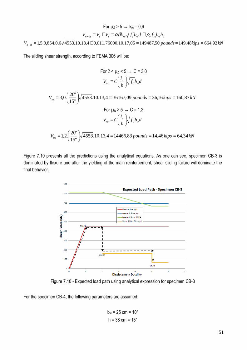
51

For µ∆ > 5 → krc = 0,6




For 2 < µ∆ < 5 → C = 3,0

dbfh

lCV wc

nns

'

=


.0,3 ===

=

For µ∆ > 5 → C = 1,2

dbfh

lCV wc

nns

'

=


.2,1 ===

=

Figure 7.10 presents all the predictions using the analytical equations. As one can see, specimen CB-3 is dominated by flexure and after the yielding of the main reinforcement, shear sliding failure will dominate the

final behavior.

Figure 7.10 - Expected load path using analytical expression for specimen CB-3


bw = 25 cm = 10"

h = 38 cm = 15"

52

d = 34 cm = 13,4"

ln = 102 cm = 40"

Asl = 2#5 = 4,0 cm2 = 0,61 in2

fyl = 517 MPa = 75 ksi = 75000 psi

Ast = #3 c/5 cm = #3 c/2"

fyt = 524 MPa = 76 ksi = 76000 psi

fc' = 30,60 MPa = 4439 psi




kNl

MV

n

yy 50,124

02,150,63.2.2

===

kNl

MV

n

uu 17,243

02,102,124.2.2 ===


ln/h = 1,02/0,38 = 2,68 → αc = 2

Acv = bw.h = 10".15" = 150 in2

ρv = Av/(bw.s) = 2.0,11/(10".2") = 0,011


kNkipspoundsVn 68,64638,14574,145387)76000.011,044392.(150 ===+=


Ec = 5600.(fc')1/2 = 5600.(30,60)1/2 = 30977,66 MPa

n = Es/Ec = 200000/30977,66 = 6,45 = m

ρ = ρ' = As/Ac = 2.2/(25.38) = 0,0042

βc = mρ'/nρ = 1,0

)1()'

.1.(2)1.()( 22ccc n

d


197,0)11.(0042,0.45,6)344

.11.(0042,0.45,6.2)11.()0042.45,6( 22 =+−+++=k


α = 3 - (0,625.ln/h) = 3 - (0,625.40"/15") = 1,33 → α=1,33 once 1,0 < α < 1,5 ρg = Asl/Ac = (4.0,31)/(10".15")=0,0082

β = 0,5 + 20.ρg = 0,5 + 20.0,0082 = 0,665 < 1,0 (ok!)

53

For µ∆ < 2 → krc = 3,5



For µ∆ > 5 → krc = 0,6




For 2 < µ∆ < 5 → C = 3,0

dbfh

lCV wc

nns

'

=


.0,3 ===

=

For µ∆ > 5 → C = 1,2

dbfh

lCV wc

nns

'

=


.2,1 ===

=

Figure 7.11 presents all the predictions using the analytical equations. As one can see, specimen CB-4 is dominated by flexure and no shear sliding or diagonal tension is expected for this specimen.


54

Table 7.2 presents the analytical failure results obtained using the equations proposed by ACI-318, FEMA 306 and ASCE/SEI 41-06.

Table 7.2 - Predicted failure results using analytical models

Shear at Flexure Failure

Diagonal Tension Strength Sliding Shear Strength Experimental Results

Vn (kN)

µ∆ < 2 µ∆ > 5 2 < µ∆ < 5 µ∆ > 5

Specimen Vy

(kN) Vu

(kN) Vn-dt (kN)

Vn-dt (kN)

Vns (kN)

Vns (kN)

Vy (kN)

Vmax (kN)

CB-1 376,07 446,27 708,47 816,54 670,53 179,49 71,79 414 478Obs

CB-2 226,66 298,43 170,29 255,13 108,35 357,33 142,93 226 275 CB-3 450,58 537,25 692,83 814,32 664,92 160,87 64,34 409 506Obs

CB-4 124,50 243,17 646,68 779,24 677,39 317,68 127,07 142 240 Observations: For specimens CB-1 and CB-3 the testes were halted before failure. The bolded values marked in the table are supposed to be the shear forces that dominated the problems. It was supposed that the rupture of the reinforcement may occur for a level of deformation that precede the sliding shear failure.

55

7.3.2 Strut-and-Tie Model and Stress Fields

SCHLAICH et al. (1987) have proposed the idea of subdividing a structure in “B-Regions” and “D-Regions”, in order to introduce rational procedures for design reinforced/prestressed concrete structures. “B-Regions” follow the “Bernoulli Hypothesis”, i.e, the hypothesis of linear deformations can be assumed through the

whole cross section, since the beginning of the loading until the failure of the section.

“B-Regions” correspond to linear members, where the stress state can be considered continuous and uniform. Also, the deformations generated by bending and axial forces are predominant when compared to the deformations caused by shear forces. For “B-Regions” the usual design procedures based on the “Beam

Theory” may be applied.

For “B-Regions”, the tensile force in the longitudinal reinforcement varies throughout the structural element, in order to balance the applied bending moment, keeping the internal level arm relatively constant. By another hand, the tensile force in the longitudinal reinforcement for “D-Regions” is likely to be constant, the internal

level arm experiences some variation and the structure presents an “arch action” behavior.

“D-Regions” presents non-linear deformations throughout the cross section and the usual design procedures based on “Beam Theory” become inadequate and even unsafe whether they are applied. In these regions, usually some details of a structure, there is a complex stress state mainly generated by shear deformations. As examples of “D-Regions” the following situations can be mentioned: pile caps, footings, deep beams,

corbels, dapped end beams and prestressed anchorages.

Generally, “D-Regions” are produced by static (loadings) and/or geometric perturbations, and the length of these discontinuity regions may be found using the Saint Venant Principle. The zones of dissipation of perturbations are usually defined based on the height of the member, as shown in the examples of Figure

7.12.

Figure 7.12 - Examples of “D-Regions” in concrete structures

(Source: ACI-318 (2005))

For “D-Regions”, usually designed in the past using rule-of-thumb rules, “Strut-and-Tie Models” or "Stress Fields Models" are desirable to apply, once these methods can provide a rational, safe and systematic procedures for design. However, for some structures, defining a strut-and-tie or a stress field model is not so straightforward and for these situations the “Finite Element Method” may be an excellent tool.

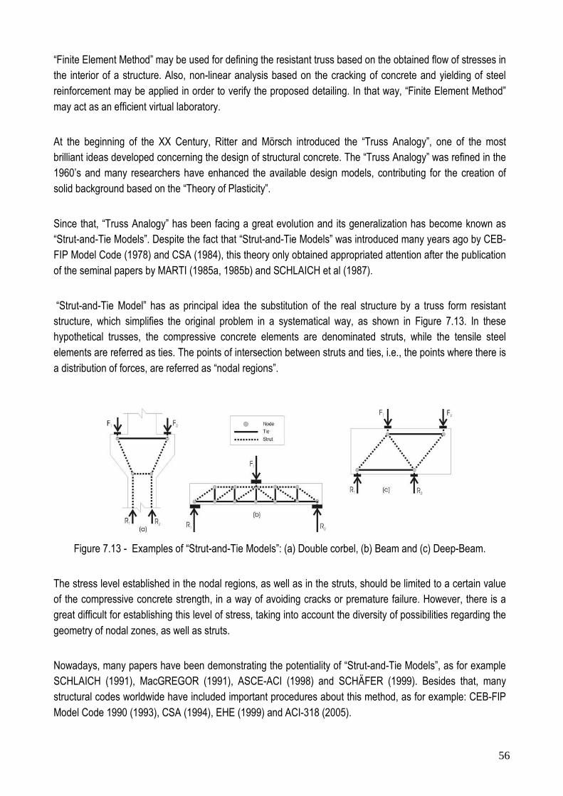
56

“Finite Element Method” may be used for defining the resistant truss based on the obtained flow of stresses in the interior of a structure. Also, non-linear analysis based on the cracking of concrete and yielding of steel reinforcement may be applied in order to verify the proposed detailing. In that way, “Finite Element Method”

may act as an efficient virtual laboratory.

At the beginning of the XX Century, Ritter and Mörsch introduced the “Truss Analogy”, one of the most brilliant ideas developed concerning the design of structural concrete. The “Truss Analogy” was refined in the 1960’s and many researchers have enhanced the available design models, contributing for the creation of solid background based on the “Theory of Plasticity”.

Since that, “Truss Analogy” has been facing a great evolution and its generalization has become known as “Strut-and-Tie Models”. Despite the fact that “Strut-and-Tie Models” was introduced many years ago by CEB-FIP Model Code (1978) and CSA (1984), this theory only obtained appropriated attention after the publication of the seminal papers by MARTI (1985a, 1985b) and SCHLAICH et al (1987).

“Strut-and-Tie Model” has as principal idea the substitution of the real structure by a truss form resistant structure, which simplifies the original problem in a systematical way, as shown in Figure 7.13. In these hypothetical trusses, the compressive concrete elements are denominated struts, while the tensile steel elements are referred as ties. The points of intersection between struts and ties, i.e., the points where there is

a distribution of forces, are referred as “nodal regions”.

Figure 7.13 - Examples of “Strut-and-Tie Models”: (a) Double corbel, (b) Beam and (c) Deep-Beam.

The stress level established in the nodal regions, as well as in the struts, should be limited to a certain value of the compressive concrete strength, in a way of avoiding cracks or premature failure. However, there is a great difficult for establishing this level of stress, taking into account the diversity of possibilities regarding the

geometry of nodal zones, as well as struts.

Nowadays, many papers have been demonstrating the potentiality of “Strut-and-Tie Models”, as for example SCHLAICH (1991), MacGREGOR (1991), ASCE-ACI (1998) and SCHÄFER (1999). Besides that, many structural codes worldwide have included important procedures about this method, as for example: CEB-FIP

Model Code 1990 (1993), CSA (1994), EHE (1999) and ACI-318 (2005).

57

At the same period of the development of "Strut-and-Tie Models", independent researchers developed in the universities of Zürich and Copenhagen an alternative approach based on the Theory of Plasticity. This alternative approach was denominated "Stress Fields Method" and has its background based on the work published by DRUCKER (1961), THÜRLIMANN et al (1975 e 1983), NIELSEN et al (1978), MARTI (1980), MUTTONI et al (1997), RUIZ & MUTTONI (2007), KOSTIC (2009) and MUTTONI et al (2011).

According to BREÑA et al (2010), stress fields were developed from direct application of the lower bound theorem of the theory of plasticity to reinforced concrete members by Drucker (1961). Original stress field models used the assumption of rigid-plastic material behavior (Figs. 7.14a,b). These stress fields, termed rigid-plastic (discontinuous) stress fields, provide safe estimates of the failure load and allow the designer to

have a clear understanding of the load-carrying mechanisms of a structure.

Application of rigid-plastic stress fields has two drawbacks. First, there is no unique solution to a given problem so a certain level of experience is needed to choose the most adequate load-carrying mechanism for a particular structure. Second, given the assumption of rigid-plastic material behavior, deformation capacity of the structural member cannot be estimated. This last drawback limits the used of rigid-plastic stress fields for solution of problems that require accurate estimates of deformation parameters such as for elements

subjected to seismic loading.

Figure 7.14 - Constitutive laws for stress field modeling: (a) rigid-plastic constitutive law for

concrete; (b) rigid-plastic constitutive law for steel; (c) elastic-plastic constitutive law for concrete; and (d) elastic-plastic constitutive law for steel (Source: BREÑA et al (2010))

In order to overcome these two limitations, elastic-plastic (continuous) stress fields have recently been developed by RUIZ & MUTTONI (2007). These models were developed assuming that materials have an elastic-plastic constitutive relation (Figs. 3c,d). With this assumption the strains in concrete and steel can be calculated and the displacements of the structural element can be determined. Since the principal strains in concrete are known, the influence of transverse strains on the compressive strength of concrete can be considered using relationships that account for reduction of compressive strength as a function of increasing

transverse strain such as the one proposed by VECCHIO & COLLINS (1986).

58

The coupling beams may be designed/verified using strut-and-tie models or stress fields. In this report, a very simple proposal is presented in order to optimize the design and verification of coupling beams. Figure 7.15 shows a linear analysis of the tested portal frame only subjected to horizontal loads from the left to the right using the package software ATENA2D. The two walls are very rigid and they both are pinned in the basis (free rotation but no horizontal or vertical displacements). As one may observe, the two walls are connected by a coupling beam and compressive (Figure 7.15.a) and tensile (Figure 7.15.b) forces act into the coupling

beam.

Figure 7.15 - Stress fields for a coupling beam connecting walls (a) compression fields and (b) tensile fields

Based on the stress fields presented in Figure 7.15, it is easy to identify a natural strut-and-tie model for the coupling beam, simply considering the efforts acting in the frontiers (M and V) of the beam. Figure 7.16 shows a first approach that can be used for the design of the coupling beam (dashed red lines indicate compression forces while solid blue line indicate tensile forces). The bending moment acting in the frontier is separated into a couple forces (M/z) and the shear is shared between two nodes. In this way the equilibrium may be

obtained and the forces acting in the single strut and in the single tie will be the same (Rc = Rt = (M/z)/sin θ

and θ = arctg (a/z)). As one can see, this forces will depend on the considered span (a) and the leverage arm

(z) considered.

Figure 7.16 - Simple strut-and-tie model for a coupling beam connecting walls

z

M/z

M/z

M/z

M/z

V/2

V/2 V/2

V/2

a

59

However, the strut-and-tie model presented in Figure 7.16 is not so easy to use in practical situations. Once horizontal and vertical reinforcement are usually mandatory in the structural codes, the presented strut-and-tie model may led to a congestion of steel in the field, especially taking into account that seismic actions will demand to put reinforcement in the strut (under seismic action there is a inversion of the presented model). For that reason, a simpler model, using orthogonal reinforcement may be preferred is some situations. Also, the majority of the buildings constructed before the 70's present orthogonal layout, in a way that is very

important to fully understand the behavior of this classical layout.

Figure 7.17 shows an alternative strut and tie model just considering orthogonal reinforcement. In this new model, the bending moments acting at the end of the coupling beam are transformed again into a couple by means of the adopted internal level arm. By another hand, shear forces are just considered acting in single nodes, in a way that a diagonal struts are necessary to carry the forces. Again, dashed red lines indicate compression forces while solid blue lines indicate tensile forces. Solid orange lines are just stabilizers

elements and they have zero or very small forces acting on them.

Figure 7.17 - Simple strut-and-tie model for a coupling beam connecting walls

Figure 7.18 shows a close-up detail of the strut-and-tie using orthogonal reinforcement. Using the equilibrium equations for the nodes it is possible to obtain the forces acting in the elements of the model. Starting the equilibrium by the node 4 it is easy to show that will be a tensile force (M/z) acting in the element between nodes 4 and 5. By symmetry, the same force will be acting in the element B between nodes 2 and 3. Also, it is possible to realize that the equilibrium of node 4 will lead to a zero force in the element C between nodes 1

and 4. By symmetry, the element C between nodes 3 and 6 will also be zero.

z

M/z

M/z

M/z

M/z

V

V

a a

60

Figure 7.18 - Detail of the strut-and-tie model for coupling beams

Now solving for the vertical equilibrium of node 1, knowing that θ = arctg (a/z), it is possible to show that

element D, between nodes 1 and 5 will be submitted to a compression force of (V/senθ). By symmetry, the

equilibrium of the node 6 will also conduct to this force to the element D between nodes 2 and 6. Solving the

horizontal equilibrium of node 1 will lead to a force of (-M/z + V.cosθ/senθ) to the element A between nodes 1

and 2. By symmetry, this same force will be acting on element A between nodes 5 and 6. Taking into

consideration that for coupling beams the angle θ will be probably varying between 45o to 65o , the

contribution provided by the shear force will be similar to the parcel provided by the moment, in a way that the

expression (-M/z + V.cosθ/senθ) will result in a very small force when compared to the forces acting in the

other elements. Finally, solving the vertical equilibrium of node 5, it is possible to show that the force acting in

element E between nodes 2 and 5 will be equal V, and this will be a tensile force.

Figure 7.19 - Forces acting in the strut-and-tie model for coupling beams

The strut-and-tie model presented in Figure 7.19 may be solved using the procedures recommended by the Appendix A of the ACI-318 (2008). BOUADI & WAHIDI (2010), for example, presented very interesting examples for coupling beams using a similar strut-and-tie model using the Appendix A of the ACI-318. It can be seen in this examples that the verification at the end of the diagonal struts is the most critical point of the model. Considering the geometry presented in Figure 7.20, a proposal for automatic design can be

developed.

2

4

1 3

5 6

A

A

B

B

C C D D E

θ θ

0

0

M/z

M/z

0 0 V

V/sen θ V/sen θ

61

Figure 7.20 - Strut-and-tie model for the design of coupling beams

The following width may be assumed for the variable w penetrating the walls:

≥

wcd

w

bfV

h

d

w

./

4/

4/

'

(Equation 7.9)

The last equation is based on the fact that there is a rigid link between the beam and the walls. In order to take into account this effect, coupling beams are usually designed considering an effective span of (ln + d), where the distance d/2 into the supports represents the hinge positions. Being d/2 the effective length, the center of the proposed strut-and-tie model will be in a distance d/4. The distance hw/4 is proposed for wall with smaller dimensions, while the term 2.Vd/fc'.bw is intended to produce a minimum length to absorb the shear force Vd. This equation is obtained using the concepts of Appendix A of ACI-318, taking into account the following deduction:

Fu < Fn

Vd < φ.0,85.βs. fc'.bw.(2w)

Vd < 0,75.0,85.0,8.fc'.bw.(2w)

w ≅ Vd / fc'.bw

The following relations are also considered in order to optimize the model:

d ≅ 0,9.h (Equation 7.10)

z ≅ 0,9.d (Equation 7.11)

a ≅ 0,5.ln + w (Equation 7.12)

θ = arc tg (z/a) (Equation 7.13)

z

M/z

M/z

M/z

M/z

V

V a a

ln hw hw

w w

h

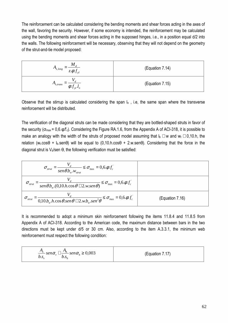
62

The reinforcement can be calculated considering the bending moments and shear forces acting in the axes of the wall, favoring the security. However, if some economy is intended, the reinforcement may be calculated using the bending moments and shear forces acting in the supposed hinges, i.e., in a position equal d/2 into the walls. The following reinforcement will be necessary, observing that they will not depend on the geometry of the strut-and-tie model proposed:

yl

dlongs fz

MA

.., φ= (Equation 7.14)

nyt

dtranss lf

VA

.., φ= (Equation 7.15)

Observe that the stirrup is calculated considering the span ln , i.e, the same span where the transverse reinforcement will be distributed.

The verification of the diagonal struts can be made considering that they are bottled-shaped struts in favor of

the security (σmax = 0,6.φ.f'c). Considering the Figure RA.1.6, from the Appendix A of ACI-318, it is possible to

make an analogy with the width of the struts of proposed model assuming that lb ≅ w and wt ≅ 0,10.h, the

relation (wt.cosθ + lb.senθ) will be equal to (0,10.h.cosθ + 2.w.senθ). Considering that the force in the

diagonal strut is Vd/sen θ, the following verification must be satisfied:

'max ..6,0

.. cstrutw

dstrut f

wbsen

V φσθ

σ =≤=

'max ..6,0

)..2cos..10,0.(. cw

dstrut f

senwhbsen

V φσθθθ

σ =≤+

=

'max2 ..6,0

...2.cos...10,0 cww

dstrut f

senbwsenhb

V φσθθθ

σ =≤+

= (Equation 7.16)

It is recommended to adopt a minimum skin reinforcement following the items 11.8.4 and 11.8.5 from Appendix A of ACI-318. According to the American code, the maximum distance between bars in the two directions must be kept under d/5 or 30 cm. Also, according to the item A.3.3.1, the minimum web

reinforcement must respect the following condition:

003,0..

≥+ hh

hv

v

v sensb

Asen

sb

A αα (Equation 7.17)

63

The following example is applied to the coupling beam designed by BOUADI & WAHIDI(2010) using the recommendations of Appendix A of the ACI-318. The following parameters are given:

Vd = 832 kN

Md = 697 kN.m

bw = 0,305 m

h = 1,829 m

ln = 1,676 m

fc' = 37,9 MPa

fyk = 420 MPa

Using the previous equations, the following parameters are calculated:

d ≅ 0,9.h = 0,9.1,829 = 1,64 m

z ≅ 0,9.d = 0,9.1,64 = 1,47 m

mw

mcmbfV

definednothh

md

w

wcd

ww 41,0

07,019,75,30.79,3/832./

4/

41,04/64,14/

'

=→

===→

==≥

a ≅ 0,5.ln + w = 0,5.1,676 + 0,41 =1,24 m

θ = arc tg (z/a) = arc tg (1,47/1,24) = 49,85o

The reinforcement needed and the verification of the diagonal strut are made as follows:

)168(05,1542.75,0.147

100.697

..2

, mmcmfz

MA

yl

dlongs φ

φ===

)145,12,1,(/75,15676,1.42.75,0

832

..2

, cmeachmmhoopStirrupsmcmlf

VA

nyt

dtranss φ

φ===

'max2 ..6,0

...2.cos...10,0 cww

dstrut f

senbwsenhb

V φσθθθ

σ =≤+

=

79,3.75,0.6,085,49.5,30.41.285,49.85,49cos.9,182.5,30.10,0

832max2

=≤+

= σσsensenstrut

!!!/70,1/47,0 2max

2 okcmkNcmkNstrut →=≤= σσ

It is recommended to adopt a minimum skin reinforcement following the items 11.8.4 and 11.8.5 from Appendix A of ACI-318. According to the American code, the maximum distance between bars in the two

directions must be kept under d/5 or 30 cm. Adopting 2φ12,5 mm each 20 cm for the horizontal direction, the

total web reinforcement will be:

64

)3181.3.3.(003,0..

−≥+ ACIfromAItemsensb

Asen

sb

Ah

h

hv

v

v αα

)3181.3.3.(003,085,4920.5,30

22,1.215,40

14.5,3022,1.2 0 −≥+ ACIfromAItemsensen o

)3181.3.3.(003,00066,00030,00036,0 −≥=+ ACIfromAItem

The following example is applied to the coupling beam designed by LEE et al (2008) using the recommendations of Appendix A of the ACI-318. The following parameters are given:

Vd = 2805 kN

Md = 1964 kN.m

bw = 0,65 m

h = 0,825 m

ln = 1,40 m

fc' = 64 MPa

fyk = 460 MPa (longitudinal) and 420 MPa (transverse)

Using the previous equations, the following parameters are calculated:

d ≅ 0,9.h = 0,9.0,825 = 0,74 m

z ≅ 0,9.d = 0,9.1,64 = 0,66 m

mw

mcmbfV

definednothh

md

w

wcd

ww 185,0

06,074,665.4,6/2805./

4/

185,04/74,04/

'

=→

===→

==≥

a ≅ 0,5.ln + w = 0,5.1,40 + 0,185 = 0,885 m

θ = arc tg (z/a) = arc tg (0,66/0,885) = 36,71o

The The reinforcement needed and the verification of the diagonal strut are made as follows:

)3211(25,8646.75,0.66

100.1964

..2

, mmcmfz

MA

yl

dlongs φ

φ===

)5,1216,2,(/60,634,1.42.75,0

2805

..2

, cmeachmmhoopsStirrupsmcmlf

VA

nyt

dtranss φ

φ===

It is recommended to adopt a minimum skin reinforcement following the items 11.8.4 and 11.8.5 from Appendix A of ACI-318. According to the American code, the maximum distance between bars in the two

directions must be kept under d/5 or 30 cm. Adopting 2φ12,5 mm each 20 cm for the horizontal direction, the

total web reinforcement will be:

65

)3181.3.3.(003,0..

−≥+ ACIfromAItemsensb

Asen

sb

Ah

h

hv

v

v αα

)3181.3.3.(003,071,3620.6522,1.2

71,365,12.65

2.4 0 −≥+ ACIfromAItemsensen o

)3181.3.3.(003,00069,0001,00058,0 −≥=+ ACIfromAItem

The proposed strut-and-tie model may be used to verify the tested coupling beams just by making some specific adjustments. For example, for Specimen CB-1, based on the geometry and reinforcement given, the

following variables may be defined:

d ≅ 34 cm

z ≅ 30 cm

ln = 51 cm

lw = 76 cm

H = 140 cm

w ≅ d/4 = 8,5 cm

a ≅ 0,5.ln + w = 0,5.51 + 8,5 = 34 cm

θ = arc tg (z/a) = arc tg (30/34) ≅ 41,42o

As,long = 6 cm2 (3#5)

fyl = 517 MPa

ful = 699 MPa

nstirrups = (ln/st)= (51/5) = 10

As,trans = 0,71.2.10 = 14,2 cm2 (#3 each 5 cm)

fyt = 524 MPa

fut = 830 MPa

In this way, the yielding of the main reinforcement may be calculated using Equation X. Observe that a

verification procedure is under investigation and for that reason φ will be assumed as one:

yl

yllongs fz

MA

.., φ=

7,51.1.306 ylM

=

mkNcmkNM yl .06,93.9306 ==

Remembering that the total force acting at the top of the walls may be calculated as Qyl = Myl.(0,5.ln+0,5.lw)/(0,25.H.ln), the predicted shear force for yielding of the main reinforcement will be Vyl = 1,1.Qyl = 364,15 kN. The rupture of the main reinforcement may be calculated in the same manner:

66

ul

ullongs fz

MA

.., φ=

9,69.1.306 ulM=

mkNcmkNMul .82,125.12582 ==

Remembering that the total force acting at the top of the walls may be calculated as Qul = Mul.(0,5.ln+0,5.lw)/(0,25.H.ln), the predicted shear force for yielding of the main reinforcement will be Vul = 1,1.Qul = 492,35 kN. The yielding of the vertical reinforcement will be:

yt

yttranss f

VA

., φ=

4,52.12,14 ytV

=

kNVyt 08,744=

In the same way, the failure of the vertical reinforcement may be estimated as:

ut

uttranss f

VA

., φ=

83.12,14 utV=

kNVut 60,1178=

The failure of the diagonal strut may be estimated as follows:

)...2.cos...10,0.(..6,0 2' θθθφ senbwsenhbfV wwcstrut +=

)42,41.20.5,8.242,41.42,41cos.38.20.10,0.(9,3.0,1.6,0 2 ooostrut sensenV +=

kNVstrut 44,436=

For Specimen CB-2, based on the geometry and reinforcement given, the following variables may be defined:

d ≅ 34 cm

z ≅ 30 cm

ln = 102 cm

lw = 72 cm

H = 140 cm

w ≅ d/4 = 8,5 cm

a ≅ 0,5.ln + w = 0,5.102 + 8,5 = 59,5 cm

θ = arc tg (z/a) = arc tg (30/59,5) ≅ 26,75o

As,long = 8,52 cm2 (3#6)

fyl = 445 MPa

ful = 694 MPa

67

nstirrups = (ln/st)= (102/16) = 6

As,trans = 0,258.2.6 = 3,1 cm2 (D4 each 16 cm)

fyt = 606 MPa

fut = 759 MPa

The yielding of the main reinforcement will be:

yl

yllongs fz

MA

.., φ=

5,44.1.3052,8 ylM

=

mkNcmkNM yl .74,113.20,11374 ==


ul

ullongs fz

MA

.., φ=

4,69.1.30452,8 ulM=

mkNcmkNM ul .38,177.64,17738 ==

Remembering that the total force acting at the top of the walls may be calculated as Qul = Mul.(0,5.ln+0,5.lw)/(0,25.H.ln), the predicted shear force for the rupture of the main reinforcement will be Vul = 0,8.Qul = 345,81 kN. The yielding of the vertical reinforcement will be:

yt

yttranss f

VA

., φ=

6,60.110,3 ytV

=

kNVyt 86,187=


ut

uttranss f

VA

., φ=

9,75.110,3 utV=

kNVut 29,235=



68


kNVstrut 86,230=


d ≅ 34 cm

z ≅ 30 cm

ln = 51 cm

lw = 76 cm

H = 140 cm

w ≅ d/4 = 8,5 cm

a ≅ 0,5.ln + w = 0,5.51 + 8,5 = 34 cm

θ = arc tg (z/a) = arc tg (30/34) ≅ 41,42o

As,long = 6,00 cm2 (3#5)

fyl = 517 MPa

ful = 699 MPa



fyt = 524 MPa

fut = 830 MPa


yl

yllongs fz

MA

.., φ=

7,51.1.3000,6 ylM

=

mkNcmkNM yl .06,93.9306 ==

Remembering that the total force acting at the top of the walls may be calculated as Qyl = Myl.(0,5.ln+0,5.lw)/(0,25.H.ln), the predicted shear force for the yielding of the main reinforcement will be Vyl = 1,1.Qyl = 364,15 kN. The rupture of the main reinforcement may be calculated in the same manner:

ul

ullongs fz

MA

.., φ=

9,69.1.3000,6 ulM=

mkNcmkNM ul .82,125.12582 ==


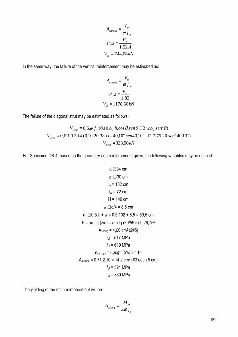
69

yt

yttranss f

VA

., φ=

4,52.12,14 ytV

=

kNVyt 08,744=


ut

uttranss f

VA

., φ=

83.12,14 utV=

kNVut 60,1178=




kNVstrut 50,328=


d ≅ 34 cm

z ≅ 30 cm

ln = 102 cm

lw = 72 cm

H = 140 cm

w ≅ d/4 = 8,5 cm

a ≅ 0,5.ln + w = 0,5.102 + 8,5 = 59,5 cm

θ = arc tg (z/a) = arc tg (30/59,5) ≅ 26,75o

As,long = 4,00 cm2 (2#5)

fyl = 517 MPa

ful = 619 MPa



fyt = 524 MPa

fut = 830 MPa


yl

yllongs fz

MA

.., φ=

70

7,51.1.3000,4 ylM

=

mkNcmkNM yl .04,62.6204 ==


ul

ullongs fz

MA

.., φ=

9,61.1.3000,4 ulM=

mkNcmkNMul .28,74.7428 ==


yt

yttranss f

VA

., φ=

4,52.12,14 ytV

=

kNVyt 08,744=


ut

uttranss f

VA

., φ=

83.12,14 utV=

kNVut 60,1178=




kNVstrut 54,182=

Table 7.3 shows the obtained results for yielding and failure of the reinforcement as well as for the diagonal strut. By another hand, Table 7.4 compares the obtained results using the proposed strut-and-tie model and the experimental results. One may observe that Specimen CB-3 would fail by shear at a shear force of 328,50 kN

71

Table 7.3 - Obtained results using the proposed strut-and-tie model

Specimen Vyl

(kN) Vul

(kN) Vyt

(kN) Vut

(kN) Vstrut (kN)

Vy,stm

(kN) Vu,stm

(kN) Predicted

Failure

CB-1 364,15 492,35 744,08 1178,60 436,44 364,15 436,44 Yielding of the

longitudinal reinforced followed by the diagonal failure

CB-2 221,74 345,81 187,86 235,29 230,86 187,86 221,74

Yielding of the transverse reinforced

followed by the yielding of the

longitudinal reinforcement

CB-3 364,15 492,35 744,08 1178,60 328,50 364,15 328,50 Failure of the diagonal strut followed by the

yielding of the longitudinal reinforced

CB-4 120,95 144,81 744,08 1178,60 182,54 120,95 144,81

Yielding of the longitudinal reinforced followed by the rupture

of the longitudinal reinforced

Observation: Vy,stm and Vu,stm are the failure loads predicted based on the obtained results

Table 7.4 - Comparison between the experimental results and the analytical results using the proposed strut-

and-tie model

Specimen Vy,stm

(kN) Vy,exp

(kN) Vy,stm / Vy,exp

Vu,stm

(kN) Vu,exp (kN)

Vu,stm / Vu,exp

CB-1 364,15 414 0,87 436,44 478 0,91 CB-2 187,86 226 0,83 221,74 275 0,80 CB-3 364,15 409 0,89 328,50 506 0,64 CB-4 120,95 142 0,85 144,81 240 0,60

Mean 0,86 Mean 0,74 SD 0,03 SD 0,14 CV 0,03 CV 0,20

72

7.4 Predictions Using Numerical Models 7.4.1 Predictions Using RESPONSE 2000

Response-2000 is a nonlinear sectional analysis program for beam-columns based on the Modified Compression Field Theory (Vecchio and Collins, 1986) developed at the University of Toronto. The program allows for axial force, bending moment, shear force, thermal and shrinkage strains, as well as time-dependent creep strains to be applied to the cross section. It is also capable of performing pushover analyses of simply supported beams up to the peak load. According to Bentz (2000), the program performs a rigorous dual-section analysis to determine the shear stress distribution on the cross section by the axial stiffness method.

According to GÜNER (2008), in sectional analysis mode, the program can predict a wide range of responses including moment-curvature, shear force-shear strain and moment-axial force interaction responses. The program has a user-friendly interface for both the model creation and results visualization, which provides ample information, encouraging more detailed investigation of the analysis results. Consequently, it is a

convenient tool for both structural engineers and researchers.

In order to perform a sectional analysis, cross section details including both the longitudinal and transverse reinforcement configurations as well as the reinforcement and concrete properties are input using the graphical interface. When the model is finalized, the analysis can be initiated through the solve menu. When the analysis is complete, the program immediately switches to a display of the analysis results. All relevant graphs can be seen in detail on the screen, and data for desired graphs can be acquired easily for further manipulation, for example, in a spreadsheet program. Also notable is the graphical representation of crack orientation and crack widths which may help the user understand the dominant behaviour of the cross section or beam member. The full version of the program, is available at www.ecf.utoronto.ca/~bentz.

Figure 7.21 - Geometric properties and materials defined for Specimen CB-1 using RESPONSE2000

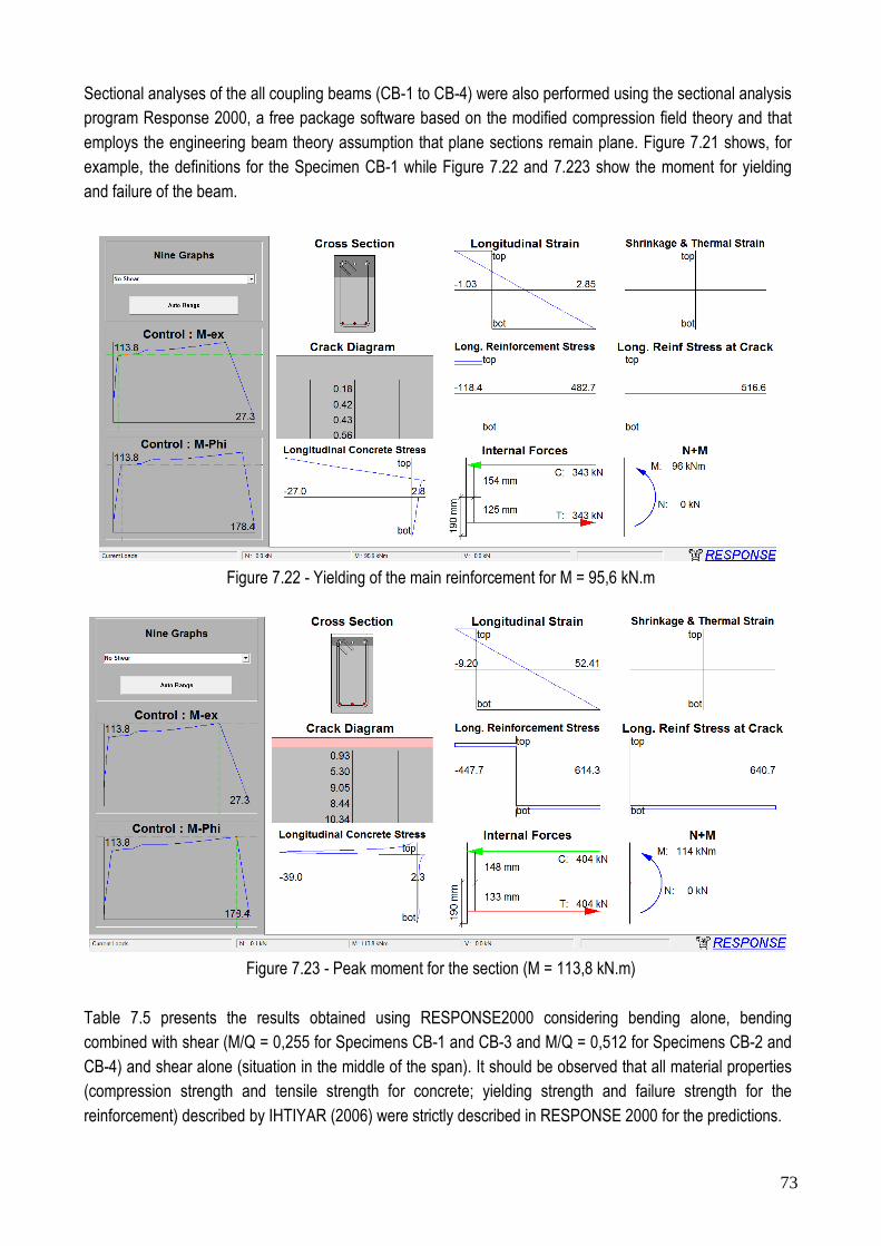
73

Sectional analyses of the all coupling beams (CB-1 to CB-4) were also performed using the sectional analysis program Response 2000, a free package software based on the modified compression field theory and that employs the engineering beam theory assumption that plane sections remain plane. Figure 7.21 shows, for example, the definitions for the Specimen CB-1 while Figure 7.22 and 7.223 show the moment for yielding and failure of the beam.

Figure 7.22 - Yielding of the main reinforcement for M = 95,6 kN.m

Figure 7.23 - Peak moment for the section (M = 113,8 kN.m)

Table 7.5 presents the results obtained using RESPONSE2000 considering bending alone, bending combined with shear (M/Q = 0,255 for Specimens CB-1 and CB-3 and M/Q = 0,512 for Specimens CB-2 and CB-4) and shear alone (situation in the middle of the span). It should be observed that all material properties (compression strength and tensile strength for concrete; yielding strength and failure strength for the

reinforcement) described by IHTIYAR (2006) were strictly described in RESPONSE 2000 for the predictions.

74

Table 7.5 - Maximum bending moments and shear forces predicted by RESPONSE2000 Supports Mid-Span

Bending alone Bending and Shear Shear Alone (M=0)

Specimen My,num

(kN.m)

Vy,num

(kN.m)

Mpeak,num

(kN.m)

Vpeak,num

(kN.m)

My,num

(kN.m)

Vy,num (kN.m)

Mpeak,num (kN.m)

Vpeak,num (kN.m)

Vy,stirrup (kN.m)

Vpeak,num

(kN.m)

CB-1 95,90 376,07 113,80 446,27 66,50 260,30 67,00 262,30 489,00 516,70

(concrete)

CB-2 115,60 225,78 152,20 297,26 77,70 151,40

(stirrup) 77,70 151,40 169,20

195,30

(concrete)

CB-3 114,90 450,58 137,00 537,25 76,50 299,70 79,60 312,00 - 451,90

(concrete)

CB-4 63,50 124,02 80,00 156,25 58,10 113,20 59,40 115,80 - 419,70

(concrete)

Observation: When not indicated the yielding and failure is supposed to happens in the main reinforcement

It is possible to realize from Table 7.5 that the combination bending and shear acting in the supports will produce the lowest shear forces and that they are very distant from the experimental results. Interestingly, if the results of bending alone acting in the supports are considered, the predictions will present more precision, as indicated in Table 7.6.

Table 7.6 - Maximum bending moments and shear forces predicted by RESPONSE2000

Bending alone Bending and Shear

Specimen Vy,test

(kN.m)

Vy,num

(kN.m)

Vy,num,/

Vy,test

Vpeak,test

(kN.m)

Vpeak,num

(kN.m)

Vpeak,num/

Vpeak,test

Vy,test

(kN.m)

Vy,num

(kN.m)

Vy,num/

Vy,test

Vpeak,test

(kN.m)

Vpeak,num

(kN.m)

Vpeak,num/

Vpeak,test

CB-1 414 376,07 0,91 478 446,27 0,93 414 260,30 0,63 478 262,30 0,55

CB-2 226 225,78 1,00 275 297,26 1,08 226 151,40

(stirrup) 0,67 275 151,40 0,55

CB-3 409 450,58 1,10 506 537,25 1,06 409 299,70 0,73 506 312,00 0,62

CB-4 142 124,02 0,87 240 156,25 0,65 142 113,20 0,80 240 115,80 0,48

Mean 0,97 Mean 0,93 Mean 0,71 Mean 0,55

SD 0,10 SD 0,20 SD 0,07 SD 0,05

CV 0,11 CV 0,21 CV 0,10 CV 0,10

75

7.4.2 Predictions Using ATENA2D

As observed by CERVENKA & CERVENKA (1996), nonlinear finite element analysis of concrete and reinforced concrete structures has been under steady development in recent decades. The worldwide research effort led to the formulation of sound constitutive models as well as numerical techniques for their implementation in computer software. These advances made possible the application of nonlinear finite element analysis in the practical engineering design. The commercial computer programs featuring nonlinear material models are offered and codes of practice are reflecting this progress. Commercially available codes allow for the analysis of entire structures, or structural members with very realistic material behavior, and a

simulation of structural performance under real loading conditions is possible.

Nonlinear finite element analysis can eliminate the inconsistency, which exists in the currently used design procedures between the internal force distribution determined from a linear elastic analysis and the section proportioning based on a nonlinear material behavior. The redistribution of internal forces due to a nonlinear material behavior is taken fully into account and a resulting stress and deformation state satisfies all three requirements of mechanics: equilibrium of forces, compatibility of deformations and material laws.

According to CERVENKA & CERVENKA (1996), the nonlinear finite element analysis is an advanced tool for design of reinforced concrete structures. If based on the smeared crack model, which is a well accepted approach, it should meet certain requirements in order to ensure a safe application. On the constitutive level the material model must be able to reproduce the failure modes important for the structural behavior under consideration. In concrete structures with extensive crack propagation the constitutive law has to describe the

nonlocal nature of the tensile fracture. This can be modeled by the fracture energy.

In this research proposal, the package software ATENA 2D, with the constitutive model SBETA was used. According to CERVENKA & CERVENKA (1996), the constitutive model in SBETA covers all important features of concrete and reinforced concrete behavior. It is based on the concept of smeared cracks, damage and fracture mechanics. The smeared concept allows to use the standard finite element technique, known well from the linear elastic analysis. Its extension to the nonlinear behavior in the pre-failure range including both material and geometrical nonlinearities is also well known and easy to implement. For this state prior to failure, SBETA uses a diffused damage concept.

The concrete failure in both, tension (cracking) and compression (crushing) causes discontinuities in the displacement fields, which are in basic disagreement with the assumptions of continuum mechanics. On the macro level concrete failure exhibits itself in the form of strain softening, and is of strongly localized nature. Therefore, special techniques based on localization limiters [8] in form of crack bands are required in order to

handle properly the post-peak behavior of concrete within the finite element model.

The reinforcement can be included in two ways, either as smeared one, or as discrete bar elements. The efficient solution techniques, pre and post-processing routines make it possible to monitor the structural behavior with all details. Large deformations, effects of temperature, shrinkage and prestressing can be also considered. According to CERVENKA & CERVENKA (2003), the material model SBETA includes the following effects of concrete behavior:

76

• non-linear behavior in compression including hardening and softening,

• fracture of concrete in tension based on the nonlinear fracture mechanics,

• biaxial strength failure criterion,

• reduction of compressive strength after cracking,

• tension stiffening effect,

• reduction of the shear stiffness after cracking (variable shear retention),

• two crack models: fixed crack direction and rotated crack direction.

Perfect bond between concrete and reinforcement is assumed within the smeared concept. No bond slip can be directly modeled except for the one included inherently in the tension stiffening. However, on a macro-level a relative slip displacement of reinforcement with respect to concrete over a certain distance can arise, if concrete is cracked or crushed. This corresponds to a real mechanism of bond failure in case of the bars with ribs. The reinforcement in both forms, smeared and discrete, is in the uniaxial stress state and its constitutive

law is a multi-linear stress-strain diagram.

The experience with the constitutive model SBETA shows, that nonlinear FE simulations can be used not only for the analysis of ultimate loads, but also for the analysis of the service conditions for crack widths, crack spacing and deflections. Although, the nonlinear analysis offers the possibility of very realistic simulation of the real structural behavior, it has been well recognized, that global analyses of large structures can be too demanding or even practically impossible. In addition, the superposition principle for the determination of the

most unfavorable load combinations cannot be used in nonlinear analysis.

Therefore, CERVENKA & CERVENKA (1996) suggest to combine linear and nonlinear analyses. A linear elastic analysis shall be used for the determination of the internal force distribution within the global structure. The critical parts shall be selected and analyzed using nonlinear analysis. In this manner, nonlinear analysis can serve as a tool for refined dimensioning. The nonlinear FE-models of local regions (such regions are in the strut-and-tie approach called as D-regions) can take into account all real factors and effects influencing the local behavior: reinforcement detailing, multi-axial interaction of stresses, fracture properties, and more. The size of this local region can be larger than the cross-section in traditional dimensioning. In practical situations, a region for nonlinear analysis can consist of structural elements (i.e. walls, beams), joints of structural elements, anchoring details, etc.

In order to investigate the coupling beams tested by IHTIYAR (2006), the package software ATENA2D was selected. Several models and solvers have been tested in the first stage using monotonic loading, in order to check the level of approximation of this approach for cyclic loading. The best results were obtained using the model SBETA combined with the Fixed Crack Model. The default parameters defined in the software were assumed in order to simulate a situation where the results are not know (practice simulation). In this way, it is possible to check the real performance of the software without manipulating so much all the huge list of parameters available in the tool. Just the compressive strength and the tensile strength of the concrete were

defined. All the other values assumed were automatically defined by the software based on the codes.

77

Figure 7.24 shows the finite element mesh, the reinforcement and the boundary conditions adopted for specimen CB-1. Horizontal loads were applied at the top of the walls and pinned supports were defined at the bottom of the walls to simulate the experimental setup. Horizontal loads and support conditions are applied in support steel plates defined along the whole width of the walls with Young’s modulus proportional to the concrete used and Poisson’s ratio 0.3.Table 7.7 presents the defined parameters for the Material SBETA, select to simulate the concrete behavior. Reinforcement properties were defined based on the experimental results using bilinear model with hardening. The problem is modeled using macroelements discretized by CCIsoQuad type elements.

1 2

X

Y

Figure 7.24 - Finite element model defined for the Specimen CB-1

Table 7.7 - Parameters defined for the SBETA Material for Specimen CB-1

Basic

Elastic modulus E 3.586e+04 MPa

Poisson's ratio µ 0,2

Tensile strength ft 2.8 MPa

Compressive strength fc -3.91e+1 MPa

Tensile

Type of tension softening Exponential

Specific fracture energy Gf 7.703e-5

Crack model Fixed

Compressive

Compressive strain at compressive strength in the

uniaxial compressive test εc

-2.181e-3

Reduction of compressive strength due to cracks 0.8

Type of compression softening Crush Band

Critical compressive displacement wd -5.0e-4 m

Shear

Shear retention factor Variable

Tension-compression interaction Linear

78

The objective of the simulation is to trace the load-displacement curve up to the post-failure softening regime. To this end, the Standard Arc-Length Method, which automatically changes the sign of load increment once a peak is attained, was selected for the simulations. To facilitate the retrieval of load-displacement curves, two monitoring point were defined. The first point monitors horizontal displacement at the corner of the left wall and the second point monitors the applied force in the same wall.

Figure 7.25 shows that the first cracks for the Specimen CB-1 occurred at the corners of the coupling beam for a total horizontal force of 57,2 kN or a shear force in the coupling beam of 62,92 kN. By another hand, Figure 7.26 shows that the first yielding was registered in the top main reinforcement (#5 bars with yielding strength of 517 MPa) at the same position where the first cracks were registered. The main reinforcement

yielded for a total horizontal force of 361,40 kN or a shear force in the coupling beam of 397,54 kN

Figure 7.25 - First cracks of specimen CB-1 for a shear force of 62,92 kN

Figure 7.26 - Yielding of the main reinforcement for a shear force of 397,54 kN

79

Figure 7.27 shows the cracking pattern for the Specimen CB-1 at the peak load and a comparison with the experimental behavior. The numerical peak load occurred for a total horizontal force of 384,20 kN or a shear force in the coupling beam of 422,62 kN. Figure 7.27 also shows the cracking regions for the concrete and crack widths just above 0,2 mm. Immediately after the peak load was registered a suddenly jump for the stresses acting in the two last stirrups (#3 bars with yielding strength of 524 MPa) situated at the right side of the beam was observed. These two stirrups started to yield for a total horizontal force of 366 kN or a shear

force in the coupling beam of 402,60 kN and the strength started to decrease for the subsequent load steps.

Figure 7.27 - Cracking pattern for a shear peak load of 402,60 kN

Figure 7.28 shows the load-displacement behavior obtained for the specimen CB-1 using monotonic loading and the nonlinear analysis resources available in the package software ATENA. As one can see, the peak load of the numerical simulation is close to the experimental failure load. By another hand, the obtained

numerical displacements are far away from the experimental response.

Figure 7.28 - Load versus displacement behavior for Specimen CB-1 using monotonic nonlinear analysis

80

The cracking behavior was firstly characterized by the degradation of the interface between the walls and the coupling beam. The first diagonal cracks appeared for a total horizontal force of 170,48 kN or a shear force in the coupling beam of 187,55 kN. After this, the diagonal cracks increased their distribution throughout the

span, however the crack widths in the interface between beam and walls were more significant.

For the specimen CB-2, the same procedures described for the specimen CB-1 were kept. The only differences were the amount of reinforcements and the material properties. Table 7.8 describes the properties

defined for the SBETA Material.


Basic





Tensile



Crack model Fixed

Compressive



-2.166e-3




Shear



Figure 7.29 shows that the first cracks for the Specimen CB-2 occurred at the corners of the coupling beam for a total horizontal force of 39,74 kN or a shear force in the coupling beam of 31,79 kN. By another hand, Figure 7.30 shows that the first yielding occurs to the stirrup for a total horizontal force of 289,40 kN or a shear force in the coupling beam of 231,52 kN. Once the D4 stirrup has a yield strength of 606 MPa, the yielding was registered in the third stirrup from left to right in the coupling beam.

Figure 7.31 shows the cracking pattern for the Specimen CB-2 at the peak load and a comparison with the experimental behavior. The numerical peak load occurred for a total horizontal force of 292,40 kN or a shear force in the coupling beam of 233,92 kN. Figure 7.31 also shows the cracking regions for the concrete and

crack widths just above 0,2 mm. The stress for the main reinforcement at the peak load was about 389 MPa.

81

Figure 7.29 - First cracks of specimen CB-2 for a shear force of 31,79 kN

Figure 7.30 - Yielding of stirrups of specimen CB-2 for a shear force of 231,52 kN


82

The cracking behavior was firstly characterized by the degradation of the interface between the walls and the coupling beam. The first diagonal cracks appeared for a total horizontal force of 157,16 kN or a shear force in the coupling beam of 125,72 kN. After this, the mentioned diagonal cracks increased their distribution throughout the span and started to increase their width until the peak load. At the failure the diagonal cracking was more intense.


numerical displacements are again far away from the experimental response.


For the specimen CB-3, the same procedures described for the specimens CB-1 and CB-2 were kept. The only differences were the amount of reinforcements and the material properties. Table 7.9 describes the

properties defined for the SBETA Material.


Basic





Tensile



83

Crack model Fixed

Compressive



-1.904e-3




Shear



Figure 7.33 shows that the first cracks for the Specimen CB-3 occurred at the corners of the coupling beam for a total horizontal force of 39,84 kN or a shear force in the coupling beam of 43,82 kN. By another hand, the first yielding occurs at the same time for the stirrups (third stirrup from the left to the right in Figure 7.34) and the main top reinforcement (Figure 7.35) for a total horizontal force of 380,60 kN or a shear force in the coupling beam of 418,66 kN. Top reinforcement bars (#5) have yield strength of 517 MPa while stirrups (#3)

have yield strength of 524 MPa.

Figure 7.33 - First cracks for specimen CB-3 for a shear force of 43,82 kN

Figure 7.34 - Yielding of the top main reinforcement of specimen CB-3 for a shear force of 418,66 kN

84

Figure 7.35 - Yielding of the stirrups of specimen CB-3 for a shear force of 418,66 kN

Figure 7.36 shows the cracking pattern for the Specimen CB-3 at the peak load. The numerical peak load occurred for a total horizontal force of 380,60 kN or a shear force in the coupling beam of 418,66 kN. Figure 7.36 also shows the cracking regions for the concrete and crack widths just above 0,2 mm. The cracking behavior was firstly characterized by the degradation of the interface between the walls and the coupling beam. The first diagonal cracks appeared for a total horizontal force of 140,56 kN or a shear force in the coupling beam of 154,61 kN. After this, the mentioned diagonal cracks increased their distribution throughout the span and started to increase their width until the peak load. At the failure the crack widths in the interface

between beam and walls were more intense.




85


For the specimen CB-4, the same procedures described for the specimens CB-1 and CB-2 were kept. The only differences were the amount of reinforcements and the material properties. Table 7.10 describes the properties defined for the SBETA Material.


Basic





Tensile



Crack model Fixed

Compressive



-1.874e-3




Shear



Miscellaneous

Specific material weight ρ 2.3e-2 MN/m3

Coefficient of thermal expansion α 1.2e-5 1/K

86

Figure 7.38 shows that the first cracks for the Specimen CB-4 occurred at the corners of the coupling beam for a total horizontal force of 38 kN or a shear force in the coupling beam of 30,40 kN. By another hand, the first yielding occurred for the main top reinforcement (Figure 7.39) for a total horizontal force of 195,46 kN or a shear force in the coupling beam of 156,36 kN. Top reinforcement bars (#5) have yield strength of 517 MPa.

Figure 7.38 - First cracks for specimen CB-4 for a shear force of 30,40 kN

Figure 7.39 - Yielding of the top main reinforcement of specimen CB-4 for a shear force of 156,36 kN

Figure 7.40 shows the cracking pattern for the Specimen CB-3 at the peak load and a comparison with the experimental behavior. The numerical peak load occurred for a total horizontal force of 281,40 kN or a shear force in the coupling beam of 225,12 kN. Figure 7.40 also shows the cracking regions for the concrete and crack widths just above 0,2 mm. No yielding was registered for the stirrups by means of the numerical

investigation.

The cracking behavior was firstly characterized by the degradation of the interface between the walls and the coupling beam. The first diagonal cracks appeared for a total horizontal force of 162,04 kN or a shear force in the coupling beam of 129,63 kN. After this, the mentioned diagonal cracks increased their distribution throughout the span while the cracks in the interface between the beam and wall started to increase their

width until the peak load. At the failure the shear sliding crack was more intense for this beam.

87





After conducting the nonlinear analysis using ATENA2D and monotonic loading for the tested specimens it is possible to observe that the numerical simulations were able to capture with reasonable precision the cracking behavior as well as the yielding and failure loads. Table 7.11 presents the obtained numerical results while Table 7.12 illustrates comparisons with the experimental results. Unfortunately, the numerical displacements were much lower than the obtained experimental results. The explanation for this difference may be on the monotonic loading adopted numerically. Once the experimental models were submitted to loading and unloading cycles, the shear degradation in the experiments is supposed to be much more

significant than that one obtained using a simple monotonic loading.

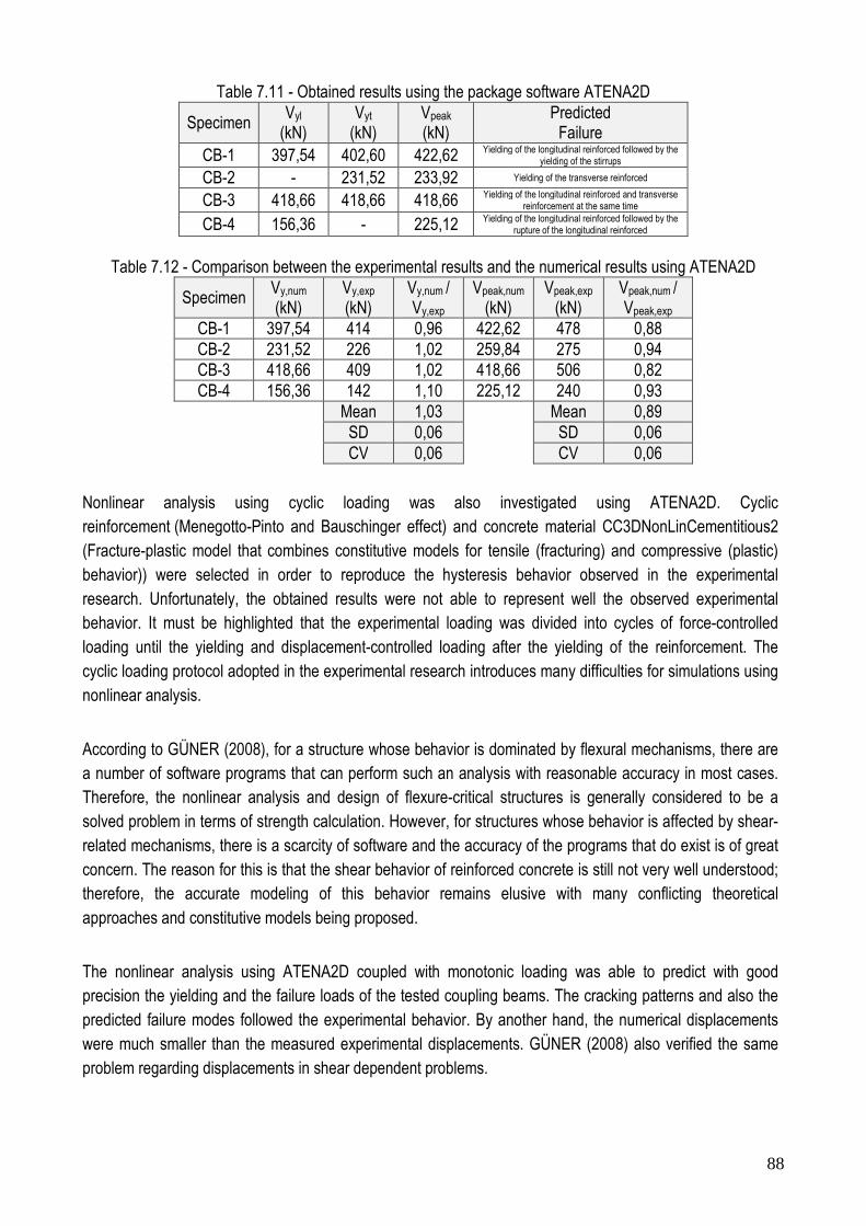
88

Table 7.11 - Obtained results using the package software ATENA2D

Specimen Vyl

(kN) Vyt

(kN) Vpeak (kN)

Predicted Failure

CB-1 397,54 402,60 422,62 Yielding of the longitudinal reinforced followed by the yielding of the stirrups

CB-2 - 231,52 233,92 Yielding of the transverse reinforced

CB-3 418,66 418,66 418,66 Yielding of the longitudinal reinforced and transverse

reinforcement at the same time CB-4 156,36 - 225,12

Yielding of the longitudinal reinforced followed by the rupture of the longitudinal reinforced

Table 7.12 - Comparison between the experimental results and the numerical results using ATENA2D

Specimen Vy,num

(kN) Vy,exp

(kN) Vy,num / Vy,exp

Vpeak,num

(kN) Vpeak,exp

(kN) Vpeak,num / Vpeak,exp

CB-1 397,54 414 0,96 422,62 478 0,88 CB-2 231,52 226 1,02 259,84 275 0,94 CB-3 418,66 409 1,02 418,66 506 0,82 CB-4 156,36 142 1,10 225,12 240 0,93


Nonlinear analysis using cyclic loading was also investigated using ATENA2D. Cyclic reinforcement (Menegotto-Pinto and Bauschinger effect) and concrete material CC3DNonLinCementitious2 (Fracture-plastic model that combines constitutive models for tensile (fracturing) and compressive (plastic) behavior)) were selected in order to reproduce the hysteresis behavior observed in the experimental research. Unfortunately, the obtained results were not able to represent well the observed experimental behavior. It must be highlighted that the experimental loading was divided into cycles of force-controlled loading until the yielding and displacement-controlled loading after the yielding of the reinforcement. The cyclic loading protocol adopted in the experimental research introduces many difficulties for simulations using nonlinear analysis.

According to GÜNER (2008), for a structure whose behavior is dominated by flexural mechanisms, there are a number of software programs that can perform such an analysis with reasonable accuracy in most cases. Therefore, the nonlinear analysis and design of flexure-critical structures is generally considered to be a solved problem in terms of strength calculation. However, for structures whose behavior is affected by shear-related mechanisms, there is a scarcity of software and the accuracy of the programs that do exist is of great concern. The reason for this is that the shear behavior of reinforced concrete is still not very well understood; therefore, the accurate modeling of this behavior remains elusive with many conflicting theoretical

approaches and constitutive models being proposed.

The nonlinear analysis using ATENA2D coupled with monotonic loading was able to predict with good precision the yielding and the failure loads of the tested coupling beams. The cracking patterns and also the predicted failure modes followed the experimental behavior. By another hand, the numerical displacements were much smaller than the measured experimental displacements. GÜNER (2008) also verified the same problem regarding displacements in shear dependent problems.

89

It must be highlighted that the chord rotations presented in the previous plots for the experimental and

numerical results were calculated using the equation θ = ∆top.(lw/ln)/hpin, proposed by BREÑA & IHTIYAR

(2011). This equation was applied once was not possible to measure directly the chord rotations in the experimental research. Other different equations were also found in the literature, as for example WHITE & ADEBAR (2004) and LEQUESNE et all (2009), indicating that there is no consensual agreement for chord rotations of coupling beams.

In fact, these mentioned proposals are numerically in the same proportion. By another hand, the mentioned equations predict values much higher than the predictions obtained using a simple frame linear elastic analysis. It looks that the proposed equations are adequate after the yielding of the reinforcement, i.e., for representing the inelastic chord rotations. Below are presented simple comparisons for specimen CB-1,

observing that the equations were adjusted to have the same notation:

BREÑA & IHTIYAR (2011)

θ = ∆top.(lw/ln)/hpin = ∆top.(760/510)/1400 = 0,00106.∆top (∆top in mm)

WHITE & ADEBAR (2004)

θ = ∆top.(lw+ln)/(hpin.ln)= ∆top.(760+510)/(1400.510) = 0,00177.∆top (∆top in mm)

LEQUESNE et all (2009)

θ = ∆top.(lw+ln)/(hpin.(ln+hb)) = ∆top.(760+510)/(1400.(510+380)) = 0,00101.∆top (∆top in mm)

SIMPLE FRAME ANALYSIS using the inertia recommended by PAULAY AND PRIESTLEY (1992):

θ = 0,000624.∆top (∆top in mm)

FEMA356 at yielding

θy = (My.ln)/(6EIb) = (95,9.100.51)/(6.3501,67.25.383/12) = 0,000203 rad

In fact, is experimentally observed that the chord rotations are usually much higher than that ones predicted using elastic models. It looks like that the chord rotations should be divided into elastic and inelastic behavior, once the adoption of the mentioned formulas seems to conduct to unrealistic values until the yielding as can

be seen in the previous calculations.

90

7.4.3 Pushover Analysis Using SAP2000

SAP2000 is a package software distributed by Computers and Structures Inc., suited for practical everyday use by office design engineers for structural analysis and design. It can perform linear-elastic static, dynamic analyses, time-history analysis and nonlinear static (pushover analysis). The static pushover analysis available in SAP 2000 is becoming a popular tool for seismic performance evaluation, once it can be viewed

as a method for predicting seismic force and deformation demands.

The pushover analysis of a structure is a static non-linear analysis under permanent vertical loads and increasing static lateral loads simulating the forces induced by earthquakes. The analysis is carried out up to failure, providing the collapse load and the ductility capacity, by means of the redistribution of internal forces that no longer can be resisted within the elastic range of structural behavior. On a building frame, the plastic rotation is monitored, and the lateral inelastic forces versus displacement response for the complete structure is analytically computed. A graph of the total base shear versus top displacement in the structure is obtained

by this analysis that may indicate any premature failure or weakness.

The main goal of a pushover analysis is to evaluate the expected performance of a structure by estimating its strength and deformation demands using a static inelastic analysis. In this way, the obtained strength and deformations demands may be compared with performance levels defined in the codes of practice. The evaluation is based on important performance parameters like: global drift, interstory drift, inelastic element deformations (absolute or normalized with respect to a yield value), deformations between elements and

element connection forces (for elements and connections that cannot sustain inelastic deformations).

According to GÜNER (2008), to perform a nonlinear static analysis of a reinforced concrete frame with SAP2000, a model of the structure is first created as if it were a linear-elastic static analysis problem. If automatic hinges are to be used, longitudinal reinforcement details should be defined including bar sizes, locations, and yield strengths. However, for the shear reinforcement, only the yield stress is required as input; neither the reinforcement ratio nor the tie or stirrup spacing is required. The next step is to assign hinges to

desired locations and it is one of the most critical phases in the nonlinear modeling process with SAP2000.

There are six default hinge options available in SAP2000: Axial (P), Torsion (T), Moment (M2 or M3), Shear (V2 or V3), Coupled (P-M2-M3), and Coupled Fibre (P-M2- M3). The hinge properties are calculated by the program for the cross section and reinforcement details provided using Tables 6-7 and 6-8 of FEMA 356 (2000). The behavior response assumed by SAP2000 for moment hinges (moment-curvature or moment-rotation relationship) and shear hinges (shear force-shear deformation relationship) is presented in Figure 7.42. Based on this curve, no plastic deformation occurs until point B where the hinge yields. This is followed by a yield plateau or strain hardening behavior until point C which represents the ultimate capacity of the hinge. After point C, the hinge’s force capacity immediately drops to point D which corresponds to the residual strength of the hinge. Point E represents the ultimate displacement capacity of the hinge after which total failure of the hinge is reached at point F. There are three stages marked between point B and C for information purposes: IO corresponds to immediate occupancy, LS to life safety, and CP to collapse prevention.

91

Figure 7.42 - Hinge behavior curve adopted in SAP2000 based on FEMA 356

Overall performance of a structure during a seismic activity is totally dependent on the performance of each component that contributes on earthquake resisting mechanism. FEMA 306 (1999) defines three discrete structural performance levels to define the condition of the structure and its components and also acceptable

chord rotations for each performance level as follows:

• Immediate occupancy performance level (IO) is defined as the post earthquake damage state in which minimal damage has occurred. Although some minor structural repairs might be needed, lateral force resisting systems didn’t lose any strength and stiffness. Risk of threatening injury is very

low;

• Life safety performance level (LS) includes damage to structural components but partial or total collapse is prevented. Possibility of a life-threatening injury due to structural damage is low.

Retrofitting of the structure might not be economically feasible;

• Collapse prevention level (CP) is defined as the state of the structure of which a significant lateral strength and stiffness was lost. Large permanent lateral deformation can be observed. However, the building should resisting gravity loads. Significant risk of injury exists and building is on the verge of collapsing with a potential aftershock.

In FEMA 356, the cyclic response of elements is represented in a simplified manner through the use of force-deformation envelopes. These envelopes are intended to capture the essential features of the nonlinear response of structural components for use primarily in nonlinear static analysis of structures. This type of structural analysis is implemented in SAP2000. According to IHTIYAR (2006), it is worth to observe that using monotonic curves to represent the cyclic response of structural components has several important limitations: (1) the effects of number of load cycles is neglected; (2) the effects of loading history and previous damage are not captured. These deficiencies are partially overcome by constructing the monotonic curves from

envelopes to experimentally measured force-deformation response of elements subjected to cyclic loading.

The general form of a force-deformation envelope provided in FEMA 356 is illustrated in Figure 7.43. As shown in this figure, the force-deformation response is constructed by defining four characteristic points along

the curve (points B through E). Determination of these values is discussed in detail in the following sections.

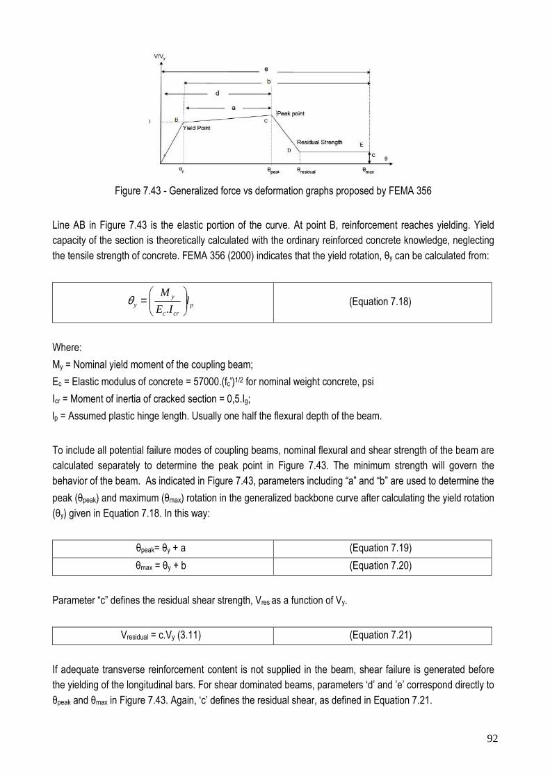
92

Figure 7.43 - Generalized force vs deformation graphs proposed by FEMA 356

Line AB in Figure 7.43 is the elastic portion of the curve. At point B, reinforcement reaches yielding. Yield capacity of the section is theoretically calculated with the ordinary reinforced concrete knowledge, neglecting the tensile strength of concrete. FEMA 356 (2000) indicates that the yield rotation, θy can be calculated from:

pcrc

yy l

IE

M

=

.θ (Equation 7.18)

Where:

My = Nominal yield moment of the coupling beam;

Ec = Elastic modulus of concrete = 57000.(fc')1/2 for nominal weight concrete, psi

Icr = Moment of inertia of cracked section = 0,5.Ig;

lp = Assumed plastic hinge length. Usually one half the flexural depth of the beam.

To include all potential failure modes of coupling beams, nominal flexural and shear strength of the beam are calculated separately to determine the peak point in Figure 7.43. The minimum strength will govern the

behavior of the beam. As indicated in Figure 7.43, parameters including “a” and “b” are used to determine the

peak (θpeak) and maximum (θmax) rotation in the generalized backbone curve after calculating the yield rotation (θy) given in Equation 7.18. In this way:

θpeak= θy + a (Equation 7.19)

θmax = θy + b (Equation 7.20)

Parameter “c” defines the residual shear strength, Vres as a function of Vy.

Vresidual = c.Vy (3.11) (Equation 7.21)

If adequate transverse reinforcement content is not supplied in the beam, shear failure is generated before the yielding of the longitudinal bars. For shear dominated beams, parameters ‘d’ and ’e’ correspond directly to

θpeak and θmax in Figure 7.43. Again, ‘c’ defines the residual shear, as defined in Equation 7.21.

93

Chord rotations FEMA 306 (1999) are defined according to component type of the structure, applied level of shear in the beam, transverse reinforcement and dominant behavior (shear of flexure). Primary components are the ones that provide the capacity of the structure to resist collapse under seismic forces and secondary elements do not contribute in the lateral resisting system. Therefore, proposed acceptable rotations of primary elements are limited than secondary elements as significant deformation of primary elements is not permitted. Conforming transverse reinforcement is defined as that consisting of closed stirrups with a maximum spacing equal to one third of the effective depth of the beam, providing a strength (Vs) at least equal to 75% of the required shear strength of the beam. In this context, just specimen CB-2 has nonconforming transverse

reinforcement. Figures 7.44 e 7.45 show the acceptable chord rotations according FEMA 306 (1999).

Figure 7.44 - Acceptable chord rotations (radians) for coupling beams controlled by flexure (FEMA 306 (1999))

Figure 7.45 - Acceptable chord rotations (radians) for coupling beams controlled by shear (FEMA 306 (1999))

According to GÜNER (2008), if there is no reinforcement defined and if no design is requested, SAP2000 uses the minimum allowable reinforcement ratios for the generation of automatic hinge properties. Generated hinge properties can be explicitly viewed and modified, if desired. For advanced users, user-defined hinges can be created. In this case, the complete flexural or shear hinge behavior of all hinges defined should be

manually supplied to the program.

The next step is to define the load application procedure (force or displacement-controlled) and nonlinear parameters (small or large displacements, P-∆ effects and hinge unloading method). Nonlinear parameters include the selection of the option "unload entire structure" which is recommended. Based on this assumption, when a hinge drops its load (i.e., reaches Point D in Figure 7.42), the entire structure is unloaded until that hinge reaches its load immediately before the load drop (i.e., Point C in Figure 7.42). The program then reverts to increasing the applied load on the whole structure; other parts of the structure may now pick up the load that was removed from the unloaded hinge. After the analysis, the load versus deflection curve can be visualized through the graphical interface or can be printed out in a data file. In addition, the hinge conditions (B, IO, LS, CP, D, and E) may be seen at each load stage using the graphical interface, which is

useful when evaluating the failure mechanism of the structure.

94

The coupling beams tested by IHTIYAR (2006) were also investigated using the pushover analysis available in the package software SAP2000. The procedures used for all the tested members are explained using the specimen CB-1 as example. The first step for conducting a pushover analysis is to construct the model in the user interface defining materials, cross sections and boundary conditions. Figure 7.46 shows the model constructed for the specimen CB-1, while Figure 7.47 and 7.50 show the definition of the materials.

Figure 7.46 - Specimen CB-1 modeled in SAP2000

Figure 7.47 - Properties of the concrete material in SAP2000

95

Figure 7.48 - Properties of the longitudinal steel reinforcement of the coupling beam

Figure 7.49 - Properties of the transverse steel reinforcement of the walls and coupling beam

96

Figure 7.50 - Properties of the longitudinal steel reinforcement of the walls

Once the material are defined, the reinforcement of the coupling beam CB-1 and the walls are created as shown in Figure 7.51 and 7.52. It must be observed that the reinforcement of the walls was approximated by an equivalent numbers of #8 bars. That was made once SAP2000 just allow the definition of one single

diameter (See Figure 7.52, "Longitudinal Bars - Rectangular Configuration")

Figure 7.51 - Definitions of the reinforcement of coupling beam CB-1

97

Figure 7.52 - Definitions of the reinforcement of the walls

The loads to be applied in the structure are defined using the path "Define, Load Patterns". As shown in Figure 7.53, two loads were created: DEAD (for simulating the self-weight of the structure) and POINT (for

simulating the lateral forces applied by the stiff loading beam used in the experimental setup).

Figure 7.53 - Definitions of the loads acting in the specimen CB-1

98

After creating the loads, the load case DEAD is set to "Nonlinear" in the "Analysis Type" by following the path "Define, Load Cases, Dead Load, Modify/Show Load Case". After, a new load case must be defined for the pushover using the path "Define, Load Cases, Dead Load, Add New Load Case". The "Nonlinear" options is selected in the box "Analysis Type" and the option "Continue from State at End of Nonlinear Case, DEAD" is selected in the box "Initial Conditions". Figures 7.54 and 7.55 illustrate the definition of the load cases and

their set to the nonlinear analysis type.

Figure 7.54 - Definitions for the dead load case

Figure 7.55 - Definitions for the pushover load case

99

From Figure 7.55 is possible to realize that the pushover load is applied selecting the load case "POINT" in the menu "Loads Applied". In the menu "Other Parameters, Load Application", the option "Displacement Control" is selected together with the option "Use Monitored Displacement" and the node at the top of the left wall (Node 3) is selected to be monitored. It is possible to observe that a maximum horizontal displacement of 10 cm was defined for the top of the walls (see the definition for "Load to a Monitored Displacement Magnitude of" in the box "Control Displacement" of Figure 7.55). Also, the results are defined to be saved for

"Multiple States" (see the definition in the box "Other Parameters" of Figure 7.55).

The next step is to associate hinges properties to the frames using the FEMA356 recommendations for beams (Table 6.7) and columns (Table 6.8). Beam and columns are selected and using the path "Assign, Frame, Hinges" the properties are defined. In this investigation, the default properties were selected and Figure 7.56 illustrates the defined hinges. As one can observe, the hinges were defined for relative distances of 0,3 and 0,7. It is made in order to have the hinges located in the interface between the walls and the coupling beam and also for taking into account the great stiffness of the wall in regarding the coupling beam. For enhancing the results, all the frames are selected and the path "Assign, Frame, Hinge Overwrites" is used to select the option "Auto Subdivide Line Objects At Hinges". This option is selected in order to discretize the

members and obtain better results.

Figure 7.56 - Definitions of the hinges for the specimen CB-1

Figure 7.57 shows the final aspect of the structure after the definitions of the hinges. As one can see, hinges were defined for the coupling beam and also for the walls. For the coupling beams, hinges were created at its extremities. For the walls, hinges were defined in the supports and also in the points were it crosses the

coupling beam.

100

Figure 7.57 - Defined hinges positions for specimen CB-1

The hinge properties are automatically created by the program based on FEMA 356 and their properties may be verified using the path "Define, Section Properties, Hinge Properties, Show Generated Props". Using the option "Show/Modify Hinges" it is possible to check the hinges properties generated. Figure 7.58 shows the

properties generated for the hinge situated in the left side of the coupling beam.

Figure 7.58 - Properties assigned for the left hinge of the coupling beam

101

Once the model is finished, the nonlinear analysis may be conducted. Once the analysis is complete the results may be verified using the path "Display, Show Deformed Shape, Push". Checking the various steps is possible to check the hinges formed with increasing displacements. Figure 7.59 shows the hinges generated throughout the load steps. For load step 1 the first hinge (yielding) is generated while for step 2 the IO (Immediate Occupancy) condition is attained. In Step 3 the residual strength is obtained while in Step 5 the

failure is finally registered.

Figure 7.59 - Evolution of hinges for specimen CB-1

Figure 7.60 - Graphical results for the hinge formed in the left side of the coupling beam

102

Using the path "Display, Show Hinge Results" is possible to check the evolution of the hinges of specimen CB-1. Selecting for example the left hinge of the coupling beam, the graphical results show in Figure 7.60 are presented. Once the hinge results are presented, tabulated results may be generated using the path "File,

Display Tables", as shown in Figure 7.61.

Figure 7.61 - Tabulated results for the hinge formed in the left side of the coupling beam

Figure 7.62 - Bending and shear forces for yielding (Step 1) and peak load (Step 2) of specimen CB-1

103

Figure 7.62 shows the bending moments and shear forces for specimen CB-1 for Step1 (Yielding) and Step 2 (Peak load). For specimen CB-1 yielding is supposed to occur for a bending moment of 99,67 kN.m (shear force in the beam of about 390,10 kN), while the peak strength is registered for a bending moment of 106,74 kN.m (shear force in the beam of about 417,78 kN). The forces acting in each step are viewed using the path "Display, Show Forces/Stresses, Frames/Cables/Tendons". Finally, using the path "Display, Show Static Pushover Curve", it is possible to check the "Resultant Base Shear vs Monitored Displacement", as shown in

Figure 7.63.

Figure 7.63 - Base shear vs monitored displacement

Conducting the same procedures presented for specimen CB-1 for the other specimens, Table 7.13 was constructed. In this table, the yielding and peak loads obtained using SAP2000 are compared with the values obtained experimentally. As one can see, the obtained results were very good for the yielding load predictions. For another hand, the failure loads were note predicted very well, especially for the beams with higher amount of shear reinforcement. In fact, when using SAP2000, there is no necessity of defining the amount of shear reinforcement. In our opinion, the available model in SAP2000 may be against safety for the

cases where shear is predominant.

Table 7.13 - Comparison between the experimental results and the numerical results using SAP2000

Specimen Vy,num

(kN) Vy,exp

(kN) Vy,num / Vy,exp

Vpeak,num

(kN) Vpeak,exp

(kN) Vpeak,num / Vpeak,exp

CB-1 390,10 414 0,94 417,78 478 0,87 CB-2 234,43 226 1,04 248,32 275 0,90 CB-3 384,55 409 0,94 411,79 506 0,81 CB-4 130,75 142 0,92 143,18 240 0,60


104

Figures 7.64 to 7.67 show the shear force vs chord rotation for the specimens using SAP2000. The results are compared with the experimental results. Point C to D in Figure 7.43 As one can see, all specimens have a very good residual strength (Point C to D in Figure 7.43) with exception of specimen CB-2 which is shear dominant. Despite the fact that SAP2000 do not requires the amount of transverse reinforcement, the software was able to identify this behavior. Of course, the user need to inform the software if the transverse

reinforcement is "conforming" or "not conforming" based on the FEMA 3006 definitions.

Figure 7.64 - Shear force vs chord rotation for specimen CB-1


105



106

7.4.4 Comparisons Among the Obtained Results

Table 7.14 illustrates the comparison between the experimental results and analytical/numerical results using different models. As one can see, RESPONSE2000 presented the best results concerning the yielding loads, even using more simple procedures than the other numerical models selected. By another hand, FEMA/ACI provided the best values regarding the peak load. One point to be observed is that every method used

conducted to conservative means of strength (except ATENA2D for yielding), which is in favor to the security.

Table 7.14 - Comparison among different models used for predicting the yielding and failure loads of the

tested coupling beams tested by IHTIYAR (2006) FEMA/ACI STM RESPONSE2000 ATENA2D SAP2000

Specimen Vy,an / Vy,exp

Vu,an / Vu,exp

Vy,stm / Vy,exp

Vu,stm / Vu,exp

Vy,num / Vy,exp

Vu,num / Vu,exp

Vy,num / Vy,exp

Vu,num / Vu,exp

Vy,num / Vy,exp

Vu,num / Vu,exp

CB-1 0,90 0,93 0,87 0,91 0,91 0,93 0,96 0,88 0,94 0,87

CB-2 0,75 0,82 0,83 0,80 1,00 1,08 1,02 0,94 1,04 0,90

CB-3 1,10 1,06 0,89 0,64 1,10 1,06 1,02 0,82 0,94 0,81

CB-4 0,87 1,01 0,85 0,60 0,87 0,65 1,10 0,93 0,92 0,60

Mean 0,91 0,96 0,86 0,74 0,97 0,93 1,03 0,89 0,96 0,80

SD 0,15 0,10 0,03 0,14 0,10 0,20 0,06 0,06 0,05 0,14

CV 0,16 0,11 0,03 0,20 0,11 0,21 0,06 0,06 0,05 0,17 The most conservative results were obtained using the proposed strut-and-tie model. However, it must be highlighted that this solution is very easy to be conducted manually and could be easily enhanced in order to get better results. Also, this model provides a more understandable procedure for the designer, once it is possible to visualize the flow of stresses inside the structure. Also, this model can be used together with the

common routines prescribed by FEMA and ACI.

The level of expertise needed for simulating the coupling beams using ATENA2D is very high and it may requires an amount of time not compatible with the deadlines to be fulfilled by a structural designer in his daily practice. Also, the huge number of parameters to be defined is supposed to generate more doubts than

certainties.

RESPONSE2000 is a very easy and powerful software to be applied in reinforced/prestressed concrete structures and it could be used together with SAP2000 in order to enhance the performance of the latter. Once RESPONSE2000 easily provides moment vs curvature graphs, it may be used to generate more accurate models for SAP2000.

It must be highlighted that all methods used in here predicted the yielding loads and failure loads using a simple monotonic analysis for a situation where cyclic loading was applied. The cyclic loading degenerates the shear strength and it is very difficult to simulate, even using powerful nonlinear resources, like that one provided by ATENA2D. In our opinion, more advance in this field is necessary in order to well predict shear

dependant structures subjected to shear degradations due cyclic loading.

107

8. DEEP BEAMS

8.1 Introduction

In reinforced concrete member such as deep beams, corbels, pile caps and walls with openings the stress distribution is highly irregular. The load carrying mechanism in these and other similar concrete elements is different than that of typical slender beams and should be designed accordingly. In the past, such members were typically designed using detailing and empirical based approaches (Schlaich et al., 1987).

In 2002 the strut-and-tie method was introduced into Appendix A of the American Concrete Institute (ACI318-02) building code as a tool for the design of structural members with stress discontinuities, or non-linear stress regions. The strut-and-tie method replaces the complex stress field with an idealized truss within the concrete member. The strut-and-tie method can help the designer understand the load carrying components in highly irregular structural elements. Knowing the bounds and limitations of the strut-and-tie method can

help designers better understand its practical applications and limitations.

According to ACI 318-05, deep beams are defined as those members with clear span not greater than four times their depth or members with concentrated forces located within twice the member depth from the support. To develop an acceptable strut-and-tie model for the design of deep beams, one must understand and identify the way shear force is transferred in deep beams.

According to ROY and BREÑA (2008), it is widely recognized that the main parameter affecting behavior of reinforced concrete beams is the shear span to effective depth ratio (a/d). Beams with an a/d of 1,0 or below transfer shear force primarily through formation of a tied arch mechanism, where concrete diagonal struts form between the point of application of load and the supports. A horizontal tie is needed to anchor these struts at their base and preserve horizontal force equilibrium at nodes located over the supports (Fig. 8(a)). By inspection, the force in this horizontal tie is constant throughout the length of the tied arch, thereby requiring that reinforcing bars develop their yield stress at the face of the nodes.

Figure 8.1 - Force transfer mechanisms in deep beams (Source: ROY and BREÑA (2008))

Still according to ROY and BREÑA (2008), truss models are generally accepted to represent behavior of beams with an a/d of 2,0 or greater. The top and bottom chords in these truss models correspond to the centroid of compression stresses and the centroid of longitudinal reinforcement of the beams, respectively. Web members in the truss model are made up of vertical ties and diagonal struts to complement the shear force transfer mechanism in the beam (Fig. 8(b)). Each vertical tie may be used for a group of transverse

108

reinforcing bars in the beam so they are commonly positioned at the centroid of the group of transverse bars they represent. Diagonal struts are used to represent compression stress fields that develop in the concrete web between diagonal cracks. The force in the horizontal tie located at the bottom of a truss model decreases in each truss panel until reaching the end of the beam. Therefore, if longitudinal reinforcement is kept constant throughout the span (as is often done in deep beams), then the anchorage demand of this

reinforcement at the end nodes is much lower than it would be if a tied arch model were used for design

The shear force transfer of deep beams with an a/d between 1,0 and 2,0 occurs by a combination of these two basic mechanisms (Fig. 8.1(c)). However, the fraction of the total force that is transferred by each mechanism, has been the source of much discussion. Most part of the codes do not prescribe recommendations on how to deal with deep beams with relations a/d between 1,0 and 2,0. ACI 318-05, for example, requires that at supports of simply supported deep beams “positive tension moment reinforcement be anchored to develop fy at the face of the support” or at the end of the extended nodal zone if the deep beam is designed using Appendix A. This implies that the assumed force transfer mechanism for deep beams

in ACI 318-05 corresponds to that of a tied arch.

Fédération International de la Précontrainte (FIP) recommendations (Fédération International de la Précontrainte Commission 3 1996) suggest that beams with a/d of approximately 0,5 or less be designed using a tied arch model, and those with an a/d of 2,0 or above be designed using a truss model. Force transfer in beams transitions from entirely tied arch action to entirely truss action as a/d increases from 0,5 to

2,0 using the following relationship:

Fz

aF

−= 12

31

1 (Equation 8.1)

where F represents the total force being transferred, F1 is the force transferred through truss action, and z is the internal lever arm (distance between top and bottom chords of the model). If, in fact, the force transfer in beams with an a/d between 1,0 and 2,0 occurs through a combination of tied arch and truss action, then the anchorage demand at the support would be reduced and the provided anchorage length of horizontal flexural reinforcement could be decreased. Furthermore, the presence of lateral confining pressures might increase the bond strength of the anchored bars permitting a reduction in required anchorage length at the support of

simply supported deep beams.

In order to investigate the combination of tied arch/truss action and the anchorage condition (possibility of anchorage length reduction) over the support of deep beams, ROY (2006), ROY & BREÑA (2008) and BREÑA & ROY (2009) tested 12 deep beams with a/d ration varying between 1,0 and 2,0. The test results indicated that beams with significantly shorter straight bar anchorage than required by ACI 318-05 (ACI Committee 318 2005) were able to transfer shear from the load point into the support. The obtained results

are investigated herein using strut-and-tie models and nonlinear analysis.

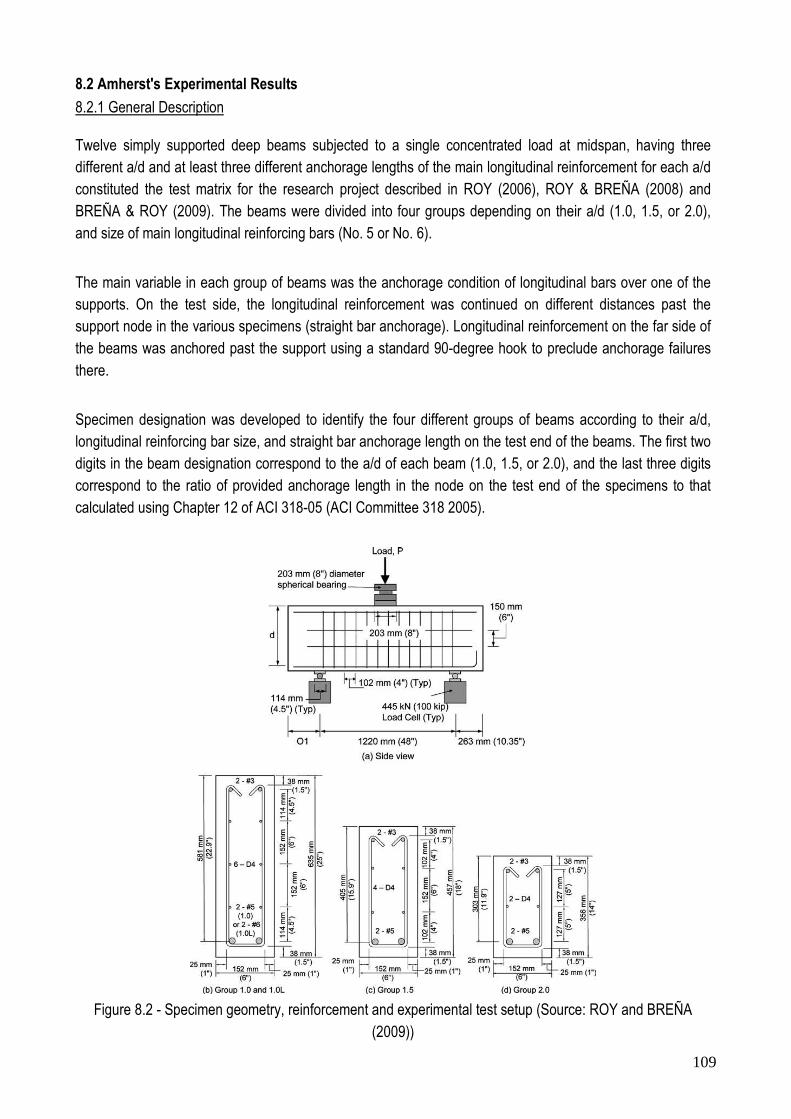
109

8.2 Amherst's Experimental Results

8.2.1 General Description Twelve simply supported deep beams subjected to a single concentrated load at midspan, having three different a/d and at least three different anchorage lengths of the main longitudinal reinforcement for each a/d constituted the test matrix for the research project described in ROY (2006), ROY & BREÑA (2008) and BREÑA & ROY (2009). The beams were divided into four groups depending on their a/d (1.0, 1.5, or 2.0), and size of main longitudinal reinforcing bars (No. 5 or No. 6).

The main variable in each group of beams was the anchorage condition of longitudinal bars over one of the supports. On the test side, the longitudinal reinforcement was continued on different distances past the support node in the various specimens (straight bar anchorage). Longitudinal reinforcement on the far side of the beams was anchored past the support using a standard 90-degree hook to preclude anchorage failures

there.

Specimen designation was developed to identify the four different groups of beams according to their a/d, longitudinal reinforcing bar size, and straight bar anchorage length on the test end of the beams. The first two digits in the beam designation correspond to the a/d of each beam (1.0, 1.5, or 2.0), and the last three digits correspond to the ratio of provided anchorage length in the node on the test end of the specimens to that calculated using Chapter 12 of ACI 318-05 (ACI Committee 318 2005).

Figure 8.2 - Specimen geometry, reinforcement and experimental test setup (Source: ROY and BREÑA

(2009))

110

Specimen nominal dimensions and reinforcing patterns are shown in Fig. 8.2. All beams had a nominal width of 152 mm (6 in.) and total depths of 635, 457, or 356 mm (25, 18, or 14 in.) for beams with a/d of 1.0, 1.5, or 2.0, respectively. Longitudinal reinforcement along the top and bottom faces of the beams consisted of deformed bars conforming to ASTM A615/615M, “Standard Specification for Deformed and Plain Carbon-Steel Bars for Concrete Reinforcement,” (ASTM International 2004). Ten of the 12 specimens had two No. 5 bars as bottom longitudinal reinforcement (Groups 1.0, 1.5, and 2.0), and the remaining two were reinforced with two No. 6 bars (Group 1.0L). An average measured yield stress of No. 5 and No. 6 bars was 492 and 469 MPa (71,4 and 68,0 ksi), respectively. An average measured peak stress of No. 5 and No. 6 bars was 758,5 and 709,5 MPa (110 and 102,9 ksi) respectively. Top reinforcement for all beams consisted of two No.

3 bars used for constructability of the beam reinforcing cage.

Web reinforcement complied with section A.3.3 in ACI 318-08 and consisted of vertical stirrups and horizontal bars formed using deformed D4 wire. Deformed wire conformed to ASTM A496/496M, “Standard Specification for Steel Wire, Deformed, for Concrete Reinforcement,” (ASTM International 2002) with an average measured yield stress equal to 605 MPa (88 ksi) and average measured peak stress equal to 643,2 MPa (93,3 ksi). The first stirrup was placed approximately 50 mm (2 in.) from the interior face of the reaction plate on each side of the beams, whereas horizontal web reinforcement extended past reaction plates. This arrangement of web reinforcement was selected to avoid having transverse reinforcement within the anchorage zone (node) of longitudinal reinforcement over the supports.

Beams were designed using a nominal compressive strength of concrete equal to 28 MPa (4 ksi) and a reinforcing steel nominal yield stress fy equal to 414 MPa (60 ksi). Just before testing each beam, specimen dimensions were verified and companion concrete cylinders were tested to determine the as-built geometry of the beams and the actual strength of concrete. Due to formwork flexibility, the actual width of the beams varied slightly from the nominal value of 152 mm (6 in.). The measured concrete compressive/tensile strength along with the as built width of each specimen at the time of testing is listed in Table 8.1. This table also shows reinforcement configuration, provided anchorage length on the test side of the beams,

cracking/yielding/peak loads and failure modes observed in the tests.

Table 8.1 - Specimen geometry and reinforcement of the deep beams tested by ROY (2006) Group

a/d Specimen

f'c

(MPa)

ft

(MPa)

b

(cm)

Main

Reinforcement

Transverse

Bars

O1

(mm)

Cracking

Load (kN)

Yielding

Load (kN)

Peak

Load (kN) Failure Mode

1.0

DB1.0-1.00 33,3 2,4 16,5 4 cm2 11-D4 54,6 165 471 677 Strut - S

DB1.0-0.75 31,7 2,7 17,3 4 cm2 11-D4 38,7 169 480 743 Strut - H

DB1.0-0.50 30,6 2,4 15,7 4 cm2 11-D4 22,2 173 476 729 Strut - H

DB1.0-0.32 27,0 2,3 15,2 4 cm2 11-D4 7,0 156 467 667 Strut - S

1.0L DB1.0-0.75L 29,9 2,7 15,5 5,68 cm2 11-D4 41,3 173 645 741 Strut - H

DB1.0-0.28L 29,4 2,8 15,5 5,68 cm2 11-D4 7,6 173 - 642 Anchorage

1.5

DB1.5-0.75 32,7 2,3 15,5 4 cm2 9-D4 29,5 107 307 459 Strut - S

DB1.5-0.50 34,1 2,4 15,2 4 cm2 9-D4 16,5 111 294 423 Strut - H

DB1.5-0.38 33,8 2,1 15,2 4 cm2 9-D4 7,0 98 294 427 Anchorage

2.0

DB2.0-0.75 34,7 2,9 15,5 4 cm2 9-D4 26,0 58 200 313 Strut - H

DB2.0-0.50 33,0 3,1 15,5 4 cm2 9-D4 11,4 67 214 297 Strut - H

DB2.0-0.43 35,6 2,6 15,5 4 cm2 9-D4 7,0 67 209 266 Anchorage

111

Longitudinal reinforcement was anchored past the support plate using either a straight bar anchorage or a hooked bar anchorage as shown in Fig. 8.2. Anchorage length of the longitudinal reinforcement was measured as the distance between the point where the bars leave the extended nodal zone (Fig. RA.1.6 in ACI 318-05), and the end of the bar as required in Section A.4.3.2 of ACI 318-05 (ACI Committee 318 2005). The end of beams where straight bar anchorages were used is denoted as the "test end", whereas the end where hooked bar anchorages were used is denoted as the "far end" of the beams. The portion of the beam extending past the support on the test end varied depending on the provided anchorage length of longitudinal reinforcement. This distance, labeled as O1 in Fig. 8.2, is listed in Table 8.1 for all specimens.

The span in all beams was equal to 1.22 m (48 in.) and specimens were subjected to a single concentrated force at midspan. Thick steel plates (25 mm [1 in.]) were placed below the loading point and above reaction points to avoid localized crushing at the nodal zones. The beam supports consisted of a pin ("far end" of beam) and a roller ("test end" of beam) in all tests. A 445 kN (100 kip) load cell was placed underneath each support to measure reactions throughout the tests and external/internal instrumentation was placed at selected locations in the specimens. All the specimen results are described in the next section, reproducing the exactly full comments of ROY (2006).

8.2.2 Specimen DB1.0-1.00

Specimen DB1.0-1.00 had longitudinal bars anchored using the full development length of 38db determined according to ACI-318. Figure 8.3 shows a picture and crack pattern of specimen DB1.0-1.00 after testing. Crack formation and extensions are marked with labels that indicate how the cracks propagated during testing. A crack (crack 1) formed at a load of about 80 kips (355,8 kN) in the tied-arch strut connecting the load point to the test node. At a load of 140 kips (622,7 kN) the middle crack (crack 2) in the beam began to significantly widen and was followed by a loud cracking sound. This sound was most likely a localized bond slippage near the crack. Peak load occurred at 152 kips (676.1 kN), and failure was the result from the crack

in the test node strut (crack 1) opening up coupled with concrete crushing in the top portion of the strut.

Figure 8.3 - Crack pattern for specimen DB1.0-1.00 (kips)

(Source: ROY (2006))

112


Figure 8.4 shows the cracking observed in specimen DB1.0-0.75. Cracking in specimen DB1.0-0.75 was similar to specimen DB1.0-1.00 except that the tied-arch strut that cracked (crack 1) was on the hooked end, and was observed at 100 kips (444,8 kN). The top of the strut on the hooked end began to crush (spall) at a load of 150 kips (667,2 kN). Failure resulted after a peak load of 166 kips (738,4 kN) from crushing in this

strut along with the crack (crack 1) along the hooked end strut opening up.

Figure 8.4 - Crack pattern for specimen DB1.0-0.75 (kips) (Source: ROY (2006))


Figure 8.5 shows the cracking pattern of specimen DB1.0-0.50. SpecimenDB1.0-0.50 differed from specimens DB1.0-1.00 and DB1.0-0.75 in that cracking was observed in both tied-arch struts. Specimen DB1.0-0.50 with an anchorage of 19db had a crack (crack 2) form at a load of 72 kips (320,5 kN) in the direct strut on the hooked node end. The strut on the test node side cracked (crack 1) at a load of 80 kips (355,8 kN). At a load of 80 kips (355,8 kN) diagonal cracks (crack 3) along the longitudinal reinforcement began forming in the test node half of the beam. The failure mechanism was crushing at the top of the hooked end strut with opening up of the crack within the same strut (crack 2). The cracking pattern in the hooked end strut

of this specimen resembled a bottle shape.


113


Specimen DB1.0-0.32 had steel reinforcement that extended 2db past the back of the node. Figure 8.6 shows the crack pattern of DB1.0-0.32. Similar to other specimens of group 1.0 no observed signs of anchorage distress were observed in the test node. Cracking was observed in both tied-arch struts as seen in specimen DB1.0-0.50. The first crack (crack 1) within a tied-arch strut occurred on the hooked end on the of the specimen at a load of about 70 kips (311,4 kN). A crack (crack 2) started in the strut on the test node end at a load of 80 kips (355,8 kN). Peak load was reached at 150 kips (667,2kN) and the failure mechanism was

observed to be crushing of the test node strut with the strut crack (crack 1) opening up.


8.2.6 Specimen DB1.0-0.75L

Specimen DB1.0-0.75L had 75% of the required development length of 38 db calculate from the anchorage length prescribed by ACI-318. Figure 8.7 shows the crack pattern for specimen DB1.0-0.75L. The first crack (crack 1) to form in a tied-arch strut occurred on the hooked end of the beam at a load of 80 kips (355,8 kN). A crack (crack 2) formed at a load of 90 kips (400,3 kN) in the strut connecting the test node. Peak load was reached at about 167 kips (742,8 kN). The failure mechanism was crushing of the hooked end strut with

opening of the hooked strut crack (crack 2).

Figure 8.7 - Crack pattern for specimen DB1.0-0.75L (kips) (Source: ROY (2006))

114

8.2.7 Specimen DB1.0-0.28L

Specimen DB1.0-0.28L had steel reinforcement that extended 2db past the back of the support providing 10.6 db of anchorage. Figure 8.8 shows the crack pattern after testing. The first observed strut crack (crack 1) occurred at a load of 90 kips (400,3 kN) in the tied-arch strut on the test node end of the specimen. No cracking was observed in the hooked end strut. At 130 kips (578,2 kN) the crack (crack 1) in the test node strut began to significantly open up. Unlike specimen DB1.0-0.75L, specimen DB1.0-0.28L failed from a lack of anchorage when a splitting crack (crack 2) formed at the test node. The peak load was 144 kips (640,5 kN). Indications of bond slip after peak load were observed from noise of the reinforcement slipping coupled

with drops in load.

Figure 8.8 - Crack pattern for specimen DB1.0-0.28L (kips) (Source: ROY (2006))


Figure 8.9 shows the cracking pattern of specimen DB1.5-0.75 after testing. The first crack (crack 1) to form within a tied-arch strut occurred in the test node strut of at a load of 70 kips (311,4 kN). The only cracking observed in the hooked end tied-arch strut was from cracks that extended into the strut at midheight of the specimen. Loud cracking sounds were heard between 60 kips (266,9 kN) and 70 kips (311,4 kN). Peak load was reached at about 103 kips (578,2 kN). Signs of strut crushing on the test node side near the top of the strut were observed as seen in Figure 8.9. The crack (crack 1) in the failed strut on the test node side

widened from the load point to the support.


115


Figure 8.10 shows the cracking pattern of specimen DB1.5-0.50. Steel reinforcement of this specimen extend 19db (11,88 in (301,75 mm)) from the extended nodal zone. Similar to specimen DB1.5-0.75 the failure mechanism was failure of the tied-arch strut. The first crack (crack 1) to form in a tied-arch strut occurred at 50 kips (222,4 kN) on the hooked end of the specimen. This crack (crack 1) continued to grow between load steps. Specimen DB1.5-0.50 observed a strut crushing failure at 95 kips (422,6 kN). The strut crushing signs came first with the crack (crack 1) in the strut opening up after. A small crack (crack 2) was observed in the

test node strut.


8.2.10 Specimen DB1.5-0.38

Specimen DB1.5-0.38 had primary a provided anchorage length that extended 2 db past the back of the support. Cracks were observed in the struts on both ends but neither fully extended through the height of the beam as in specimens DB1.5-0.75, and DB1.5-0.50. Development distress was first observed in bond slip cracks between 70 kips (311,4 kN) and 85 kips (378,1 kN). A large amount of cracking (crack 1) and ultimate bond failure was observed between 92 kips (409,.2 kN) and 93 kips (413,7 kN) with the sound of the longitudinal reinforcement slipping in the concrete. The result was a load dropped to 84 kips (373,6 kN). The observed failure mode was an anchorage failure from lack of bond of the longitudinal reinforcement as shown

in Figure 8.11.


116

8.2.11 Specimen DB2.0-0.75

Figure 8.12 shows the cracking pattern for specimen DB2.0-0.75. The first crack (crack 1) in a tied-arch strut formed in the hook end strut at a load of 30 kips (133,4 kN) and continued to grow during testing. Cracks continued into the tied-arch strut on the test node end. At 50 kips (222,4kN) a crack (crack 2) was observed in the test node strut originating from the support. The failure mode was observed to be strut failure in the hook end of the beam as seen in Figure 8.12. There was little localized crushing (spalling) in the hook side near the top node.


8.2.12 Specimen DB2.0-0.50

Observed cracking pattern for specimen DB2.0-0.50 is presented in Figure 8.13. Specimen DB2.0-0.50 formed its first tied-arch strut crack (crack 1) in the test node strut at a load of 40 kips (177,9 kN). The hook end strut did not have any cracks running along its length but did have cracks continue into it. It took a long time to load from 50 kips (222,4 kN) to 55 kips (244,6 kN), similar to specimen DB2.0-0.50. There was a loud sound suggesting some anchorage distress at 58 kips (258,0 kN), and again at 62 kips (275,8 kN). The second sound was coupled with a load drop to 57 kips (253,5 kN). Similar noises with small drop in load were heard again at 63 kip (280,2 kN) and 64 kips (284,7 kN). The failure mode was observed to be strut failure in the test node strut of the beam. There was more crushing (spalling) along this strut than in specimen DB2.0-

0.75.


117

8.2.13 Specimen DB2.0-0.43

Figure 8.14 shows the crack pattern for specimen DB2.0-0.43. Specimen DB2.0-0.43 exhibited debonding (crack 1) at 60 kips (266,9 kN). No debonding sounds were heard but loss of strain was coupled with a drop in load. A large amount of cracking was observed long the reinforcement over the support.


8.3. Specimen Deflections

According to ROY (2006), four types of failure behavior were observed in the load-deflection response. In specimens that exhibited strut failures, two types of load-deflection failure responses were observed. Ductile failures were observed in specimens DB1.0-0.75, DB1.0-0.50, DB2.0-0.75, and DB2.0-0.50. Brittle failures (in respect to the other strut failures) were observed in specimen DB1.0-1.0, DB1.0-0.32, DB1.0-0.75L, DB1.5-

0.75, and DB1.5- 0.50. In the three specimens that showed anchorage failures two types of load-deflection

responses were observed at failure. Specimen DB1.0-0.32L showed a brittle load-deflection failure response and failed from splitting in the concrete. Specimens DB1.5- 0.38, and DB2.0-0.43 failed from bond loss and

showed a more ductile failure. Figures 8.15 to 8.18 present the load-deflection behavior for the specimens.

Figure 8.15 - Load-deflection for specimens from Group 1 (Source: ROY (2006))

118

Figure 8.16 - Load-deflection for specimens from Group 1L (Source: ROY (2006))

Figure 8.17 - Load-deflection for specimens from Group 1.5 (Source: ROY (2006))

Figure 8.18 - Load-deflection for specimens from Group 2 (Source: ROY (2006))

119

8.4 Analytical Analysis Using Strut-And-Tie Model

In order to investigate the experimental results, the simple strut-and-tie model presented in Figure 8.19 is proposed. Using the procedures recommend by the Appendix A of ACI-318, it is possible to obtain the analytical yielding and failure loads. In this model, the major problem is the determination of the height of the top horizontal strut (htop). Once this value is known all the other parameters may be easily found. In order to show how the proposed verification model works, the deep beam DB1-1.00 tested by ROY (2006) is

presented.

Figure 8.19 - Simple strut-and-tie model used to investigate the deep beam tested by ROY (2006))

The following data is known for the deep beam DB1-1.00:

As = 4,0 cm2

fy = 492 MPa

fu = 758,5 MPa

a = 56 cm

b = 16,5 cm

d = 58,1 cm

f'c = 33,3 MPa

wt = 2.(h-d) = 2.5,40 = 10,80 cm

lb bottom plate = 11,4 cm

lb top plate = 20 cm

lbeam = 122 cm

Q = P/2

Using equilibrium conditions for the bottom node it is easy to show that:

Fs = Q/sinα (force in the diagonal strut)

Ft = Fs.cosα (force in the tie)

120

The yielding force for the main tie may be calculated by:

Ft = As.fy = 4.49,2 = 196,80 kN

Assuming that the force in the top strut (Fc) must be equal to the maximum force in the tie (horizontal equilibrium), it is possible to find the height (htop) of the top node and the shear force that generates yielding of the main tie:

Ft = Fc = 196,80 kN

Fns = fce.Acs = 0,85.βs.f'c.b.htop

htop = Fc / (0,85.βs.f'c.b)

βs = 1,00 (prismatic strut in the top)

htop = 196,80 / (0,85.1.3,33.16,5) = 4,21 cm

z = d - htop/2 = 58,1 - 4,21/2 = 56 cm

α = arc tg (z/a) = arc tg (56/56) = 45o

Ft = Fs.cosα → Fs = Ft/cosα = 196,80/cos 45o = 278,32 kN

Fs = Q/sinα → Q = Fs.sinα = 278,32.sin 45o = 196,80 kN

Q1 = P1/2 → P1 = Q1.2 = 196,80.2 = 393,60 kN (Yielding load)

Once the htop is determined, it is possible to conduct verifications in all other positions (nodes, struts, etc)

using the ACI-318 prescriptions. The CCT bottom node (βn = 0,80) is evaluated as follows and as one can

check the failure of this node is governed by the tie for a total load P = 807,04 kN:

Fnn = fce.Anz = 0,85. βn. f'c.Anz = Q

Reaction force →

Q2 = 0,85.βn. f'c.b.lbottom = 0,85.0,80.3,33.16,5.11,4 = 425,93 kN

P2 = 2.Q2 = 851,86 kN

Tie →

Q3 = 0,85.βn. f'c.b.wt = 0,85.0,80.3,33.16,5.10,80 = 403,52 kN

P3 = 2.Q3 = 807,04 kN

Diagonal strut →

wbottom = lbottom.sinα + wt.cosα = 11,4.sin 45o + 10,80.cos 45o = 15,70 cm

Q4 = 0,85.βn. f'c.b.wbottom = 0,85.0,80.3,33.16,5.15,70 = 586,59 kN

P4 = 2.Q4 = 1173,18 kN

121

The CCC top node (βn = 1,00) is evaluated as follows and as one can check the failure of this node is

governed by the horizontal strut for a total load P = 393,24 kN:


Reaction force →

Q5 = 0,85.βn. f'c.b.lbottom = 0,85.1,00.3,33.16,5.10 = 467,03 kN

P5 = 2.Q5 = 934,06 kN

Horizontal strut →

Q6 = 0,85.βn. f'c.b.htop = 0,85.1,00.3,33.16,5.4,21 = 196,62 kN

P6 = 2.Q6 = 393,24 kN

Diagonal strut →

wtop = ltop.sinα + htop.cosα = 10.sin 45o + 4,21.cos 45o = 10,05 cm

Q7 = 0,85.βn. f'c.b.wtop = 0,85.1,00.3,33.16,5.10,05 = 469,37 kN

P7 = 2.Q7 = 938,74 kN

The diagonal strut (βs = 0,75) is evaluated as follows:

Fns = fce.Acs = 0,85. βn. f'c.Acs = 0,85. βn. f'c.b.wtop

Fs = 0,85.0,75.3,33.16,5.10,05 = 352,03 kN

Q8 = Fs.sinα = 352,03.sin 45o = 248,92 kN

P8 = 2.Q8 = 497,85 kN

The horizontal strut (βs = 1,00) is evaluated as follows:

Fns = fce.Acs = 0,85. βn. f'c.Acs = 0,85. βn. f'c.b.htop

Fc = 0,85.1,00.3,33.16,5.4,21 = 196,62 kN

Q9 = Fc.sinα/cos α = 352,03.sin 45o/cos 45o = 196,62 kN

P9 = 2.Q9 = 393,24 kN

It must be highlighted that the maximum loads obtained for the diagonal and horizontal struts as well some nodes may be not realistic in some situations, especially if they are dependent on htop. For simplicity, htop was determined based on the yielding force acting in the main tie and for a real situation this height can be higher if demanded. Assuming a bilinear behavior for the reinforcement, once the main tie starts to yield htop may increase until the ultimate force in the reinforcement is reached. In this way, it is interesting to calculate the maximum loads when the tie is also subjected to ultimate forces, objecting to find more realistic failure loads. By another hand, failure loads obtained for some directions in the nodes, that are not dependant on htop

122

(reaction in the plates or tie width), may be assumed as governing the strength of the nodes if their result is lower than for the positions depending on htop. The calculations assuming the possibility of a high value for

htop based on the ultimate strength of the main reinforcement is present as follows:

The ultimate force for the main tie may be calculated by:

Ft = As.fu = 4.75,85 = 303,40 kN

Assuming that the force in the top strut (Fc) must be equal to the maximum force in the tie (horizontal equilibrium), it is possible to find the height (htop) of the top node and the shear force that generates yielding of the main tie:

Ft = Fc = 303,40 kN

Fns = fce.Acs = 0,85.βs.f'c.b.htop

htop = Fc / (0,85.βs.f'c.b)

βs = 1,00 (prismatic strut in the top)

htop = 303,40 / (0,85.1.3,33.16,5) = 6,50 cm

z = d - htop/2 = 58,1 - 6,50/2 = 54,85 cm

α = arc tg (z/a) = arc tg (54,85/56) = 44,41o

Ft = Fs.cosα → Fs = Ft/cosα = 303,40/cos 44,41o = 424,72 kN

Fs = Q/sinα → Q = Fs.sinα = 424,72.sin 44,41o = 298,80 kN

Q1 = P1/2 → P1 = Q1.2 = 298,80.2 = 597,60 kN (ultimate load)

Once the htop is determined, it is possible to conduct verifications in all other positions (nodes, struts, etc)

using the ACI-318 prescriptions. The CCT bottom node (βn = 0,80) is evaluated as follows and as one can

check the failure of this node is governed by the tie for a total load P = 807,04 kN:


Reaction force →

Q2 = 0,85.βn. f'c.b.lbottom = 0,85.0,80.3,33.16,5.11,4 = 425,93 kN

P2 = 2.Q2 = 851,86 kN

Tie →

Q3 = 0,85.βn. f'c.b.wt = 0,85.0,80.3,33.16,5.10,80 = 403,52 kN

P3 = 2.Q3 = 807,04 kN

Diagonal strut →

wbottom = lbottom.sinα + wt.cosα = 11,4.sin 44,1o + 10,80.cos 44,1o = 15,69 cm

123

Q4 = 0,85.βn. f'c.b.wbottom = 0,85.0,80.3,33.16,5.15,69 = 586,22 kN

P4 = 2.Q4 = 1172,44 kN

The CCC top node (βn = 1,00) is evaluated as follows and as one can check the failure of this node is

governed by the horizontal strut for a total load P = 607,14 kN:


Reaction force →

Q5 = 0,85.βn. f'c.b.lbottom = 0,85.1,00.3,33.16,5.10 = 467,03 kN

P5 = 2.Q5 = 934,06 kN

Horizontal strut →

Q6 = 0,85.βn. f'c.b.htop = 0,85.1,00.3,33.16,5.6,50 = 303,57 kN

P6 = 2.Q6 = 607,14 kN

Diagonal strut →

wtop = ltop.sinα + htop.cosα = 10.sin 44,1o + 6,50.cos 44,1o = 11,63 cm

Q7 = 0,85.βn. f'c.b.wtop = 0,85.1,00.3,33.16,5.11,63 = 543,16 kN

P7 = 2.Q7 = 1086,32 kN

The diagonal strut (βs = 0,75) is evaluated as follows:

Fns = fce.Acs = 0,85. βn. f'c.Acs = 0,85. βn. f'c.b.wtop

Fs = 0,85.0,75.3,33.16,5.11,63 = 407,37 kN

Q8 = Fs.sinα = 407,37.sin 44,1o = 283,49 kN

P8 = 2.Q8 = 566,99 kN

The horizontal strut (βs = 1,00) is evaluated as follows:

Fns = fce.Acs = 0,85. βn. f'c.Acs = 0,85. βn. f'c.b.htop

Fc = 0,85.1,00.3,33.16,5.6,50 = 303,57 kN

Q9 = Fc.sinα/cos α = 303,57.sin 44,1o/cos 44,1o = 294,18 kN

P9 = 2.Q9 = 588,36 kN

124

Table 8.1 resumes the maximum analytical loads using the proposed strut and tie-model, taking into account that the height of the top horizontal strut is determined based on the yielding or ultimate force of the main tie. As one can see, the proposed model is able to predict the yielding of the main reinforcement for a load of

393,60 kN. The failure load is predicted to occur at the diagonal strut at the top node for a load of 566,99 kN.

Table 8.1 - Predicted yielding and failure loads using the proposed strut-and-tie model

Yielding of Reinforcement Failure of Reinforcement Predicted failure

Position Pmax (kN) Pmax (kN)

Tie 393,60 597,60 Yielding of the main reinforcement

followed by the failure of the

diagonal strut in the top node

Bottom Node 807,04 (wt dependent) 807,04

Top Node 393,24 (htop dependent) 607,14

Diagonal Strut 497,85 (htop dependent) 566,99

Horizontal Strut 393,24 (htop dependent) 588,36

The routine presented previously was programmed into the Matlab package software and the routine can be seen in the Appendix A of the present work. Table 8.2 presents the obtained results using the written code.

Table 8.2 - Comparison between experimental results and analytical results for the deep beams tested Experimental STM Experimental STM Yielding Peak

Specimen Yielding Load

(kN) Yielding Load

(kN)

Peak Load

(kN)

Peak Load

(kN) PSTM/Pexp PSTM/Pexp

DB1.0-1.00 471 393,55 677 570,52 0,84 0,84

DB1.0-0.75 480 393,52 743 569,83 0,82 0,77

DB1.0-0.50 476 391,42 729 524,76 0,82 0,72

DB1.0-0.32 467 388,53 667 478,27 0,83 0,72

DB1.0-0.75L 645 - 741 681,52 - 0,92

DB1.0-0.28L - - 642 669,33 - 1,04

DB1.5-0.75 307 268,29 459 399,94 0,87 0,87

DB1.5-0.50 294 268,96 423 401,54 0,91 0,95

DB1.5-0.38 294 268,82 427 401,21 0,91 0,94

DB2.0-0.75 200 197,84 313 292,37 0,99 0,93

DB2.0-0.50 214 197,06 297 290,51 0,92 0,98

DB2.0-0.43 209 197,93 266 292,58 0,95 1,10

Mean 0,89 0,90

SD 0,06 0,12

CV 0,07 0,13

As one can see, the proposed strut-and-tie model was able to provide good predictions regarding the yielding and failure loads for the specimens tested by ROY(2006). One point that must be highlighted in here is that the complementary horizontal reinforcement was not included in the model. In this way, the presented strut-and-tie model could be enhanced in order to account for these reinforcement, as they contribute to final

strength of the diagonal struts and delay the yielding of the main reinforcement.

125

A tied-arch strut and tie model consistent with the peak measured load in the tests was also proposed by BREÑA & ROY (2009), based on the paper published by WIGHT and PARRA-MONTESINOS (2003), where the strut inclination angle and width are determined iteratively. In this model, the geometry of the tied-arch model was established so that node strength was observed in the nodal region of the beam, as shown in Figure 8.20.

Figure 8.20 - Model and node geometry used for strut strength evaluation (BREÑA & ROY (2009))

From symmetry of the test setup, the total applied force on the beams resulted in equal shear force transferred to each support. The force in the direct strut forming between load and support in the tied-arch

model is FS = V/sinα, where α is the angle of inclination of the strut measured from horizontal (Fig. 8.20). The

angle α depends on the horizontal distance between the resultant of one-half of the applied force and the

support (560 mm [22 in.]), and the vertical distance between the top and bottom chords in the model (z).

The top-node height hnode-top was initially assumed equal to 50 mm (2 in.) to initiate iterations. After

determining FS for the initial α, the top horizontal compressive force was calculated as FC = FS cosα; this

force was then equated to the nominal strength of the top node given by Fnn = fce.Anz = 0,85.βn.fc'.Anz with βn =

1,0 to solve for the required top-node height to avoid node crushing, as follows:

αα

tan85,085,0cos

'' bf

V

bf

F

bf

Fh

cc

S

ce

Ctopnode ===−

The depth between top and bottom chords in the model, z, was then revised and a new strut angle α was

determined to avoid nodal failure:

126

2topnodeh

dz −−=

Iterations were conducted until hnode-top was approximately the same in two subsequent calculation cycles. In all iterations, the height of the bottom node was assumed equal to 102 mm (4 in.), twice the distance between the bottom face of the beams and the centroid of the bottom longitudinal reinforcement. Once convergence was achieved and an appropriate strut inclination was found, the top and bottom widths of the strut were

determined from:

wstrut = Lplatesinα + hnodecosα

where the plate widths and node heights used for the top and bottom nodes in the previous equation corresponded to those shown in Fig. 8.20 (a). Because the bottom plate is wider than half the top plate, the top end of the strut ended up governing strut strength in all the specimens. This is consistent with the location of observed concrete spalling near the top of the struts in all specimens that failed by strut crushing. The

stress at the top end of the strut was then calculated using the following equation:

bw

Ff

tops

Sstrut

−

=

where the as-built width of the specimens, b, was used and ws-top is the width of the strut determined before at the top node. In order to show the development of the proposed approach, beam DB1-1.00 was selected to

illustrate the calculations:

Deep Beam DB1-1.00

Pfailure = 676 kN (failure load)

Vfailure = 338 kN (reaction failure load)

a = 56 cm

d = 58,1 cm

fc' = 33,3 MPa

b = 16,5 cm

ws = 10,8 cm (width of the main tie)

hnode-top = 5 cm (estimated for the first iteration)

Lplate, bottom = 11,4 cm

Lplate, top = 20,2 cm

127

First Iteration:

cmh

dz topnode 60,5525

1,582

=−=−= −

oarca

zarc 79,44

5660,55

tantan ===α

kNV

F oS 77,47979,44sin

338sin

===α

kNFF oSC 49,34079,44cos.77,479cos === α

nzcens AfF .=

'..85,0 cnce ff β=

topnodecnnzcnns hbfAfF −== ....85,0...85,0 '' ββ

cmbf

F

bf

Fh

cn

C

ce

Ctopnode 29,7

5,16.33,3.00,1.85,049,340

85,0 ' ====− β

Second Iteration:

cmh

dz topnode 46,54229,7

1,582

=−=−= −

oarca

zarc 20,44

5646,54

tantan ===α

kNV

F oS 20,48420,44sin

338sin

===α

kNFF oSC 33820,44cos.20,484cos === α

cmbf

F

bf

Fh

cn

C

ce

Ctopnode 24,7

5,16.33,3.00,1.85,0338

85,0 ' ====− β

Third Iteration:

cmh

dz topnode 50,54224,7

1,582

=−=−= −

oarca

zarc 22,44

5650,54

tantan ===α

kNV

F oS 65,48420,44sin

338sin

===α

kNFF oSC 33822,44cos.65,484cos === α

cmbf

F

bf

Fh

cn

C

ce

Ctopnode 24,7

5,16.33,3.00,1.85,0338

85,0 ' ====− β(Convergence attained)

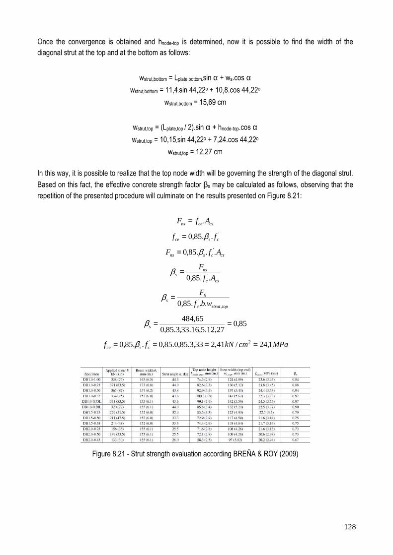
128

Once the convergence is obtained and hnode-top is determined, now it is possible to find the width of the diagonal strut at the top and at the bottom as follows:

wstrut,bottom = Lplate,bottom.sin α + ws.cos α

wstrut,bottom = 11,4.sin 44,22o + 10,8.cos 44,22o

wstrut,bottom = 15,69 cm

wstrut,top = (Lplate,top / 2).sin α + hnode-top.cos α

wstrut,top = 10,15.sin 44,22o + 7,24.cos 44,22o

wstrut,top = 12,27 cm

In this way, it is possible to realize that the top node width will be governing the strength of the diagonal strut.

Based on this fact, the effective concrete strength factor βs may be calculated as follows, observing that the

repetition of the presented procedure will culminate on the results presented on Figure 8.21:

cscens AfF .=

'..85,0 csce ff β=

cscsns AfF ...85,0 'β=

csc

nss Af

F

..85,0 '=β

topstrutc

Ss wbf

F

,' ...85,0

=β

85,027,12.5,16.33,3.85,0

65,484 ==sβ

MPacmkNff csce 1,24/41,233,3.85,0.85,0..85,0 2' ==== β

Figure 8.21 - Strut strength evaluation according BREÑA & ROY (2009)

129

8.5 Nonlinear Analysis Using ATENA2D

In order to investigate the deep beams tested by ROY (2006), the package software ATENA2D was selected. Several models and solvers have been tested and the best results were obtained using the model SBETA combined with the Fixed Crack Model. The default parameters defined in the software were assumed in order to simulate a situation where the results are not know (practice simulation). In this way, it is possible to check the real performance of the software without manipulating so much all the huge list of parameters available in the tool. Just the compressive strength and the tensile strength of the concrete were defined. All the other values assumed for concrete were automatically defined by the software based on the codes.

1

2X

Y

Figure 8.22 - Finite element model defined for the Specimen DB1-1.0

Table 8.3 - Parameters defined for the SBETA Material for Specimen DB1-1.0

Basic





Tensile



Crack model Fixed

Compressive



-1.973e-3




Shear



130

Figure 8.22 shows the finite element mesh, the reinforcement and the boundary conditions adopted for specimen DB1-1.0. The problem is modeled using macroelements discretized by CCIsoQuad type elements. Vertical point load was applied at the top of the deep beam and pinned supports were defined at the bottom in order to simulate the experimental setup. Vertical loading and support conditions are applied in support steel plates with Young’s modulus of 210 GPa and Poisson’s ratio 0,3.Table 8.3 presents the defined parameters

for the Material SBETA, select to simulate the concrete behavior.

Reinforcement properties were defined based on the experimental results using bilinear model. In most practical cases the bond is not a significant effect because the bond strength is only seldom reached. However, in the present investigation, reduced anchorage length was applied and bond strength needs to be evaluated. For this reason, adherence based on the bond model of BIGAJ (1999) was defined for the main tie (bars number #5 and #6) while the other reinforcement were defined without bond model (option perfect

connection).

The basic property of the reinforcement bond model is the bond-slip relationship and it defines the bond strength depending on the value of current slip between reinforcement and surrounding concrete. The brittle behavior of the Bigaj’s model is attributed to the splitting mode of bond behavior and is more realistic then the plastic behavior. The slip law for this model depends on the bond quality (poor, good, very good), concrete cubic compressive strength and reinforcement bar radius as shown in Figure 8.23. The present bond model in ATENA2D is not directly dependent on confinement caused by the normal stresses acting on planes parallel

with the reinforcement direction.

Figure 8.23 - Bond law by BIGAJ (1999)

Loading is applied by prescribing vertical displacement at the middle point on top of the loading plate in constant increments of 0,1 mm. The Newton-Raphson solution method is selected and the overall response is recorded at two monitoring points – loading as the reaction at the top loading point and deflection at the

bottom of the beam on the symmetry plane.

Figure 8.24 shows the first cracks for the specimen DB1-1.0. As one can see, the flexural cracks appeared for a point load of about 160 kN and the maximum stress in the main tie for this moment is about 126 MPa. Figure 8.25 shows the cracking pattern when the main tie starts yielding for a point load of 674 kN. As one

can see, diagonal cracks are already very intense for this load level.

131

Figure 8.24 - First cracks for the specimen DB1-1.0

Figure 8.25 - Cracking pattern (w>0,2 mm) for the yielding of the main tie of specimen DB1-1.0

Figure 8.26 - Experimental failure and predicted numerical failure for specimen DB1-1.0

132

Figure 8.26 shows a comparison between the experimental failure and the predicted failure using ATENA2D. It is possible to observe that the cracking pattern is very similar, though no crushing was observed in the top plate using ATENA2D. The cracking and failure load were both well predicted while the yielding load kept far away from the experimental observation. In the experimental analysis, reinforcement yielded but the specimen presented an additional strength until the failure. In the numerical prediction, the reinforcement yielded and failure came immediately after. Figure 8.27 shows the force versus displacement obtained

numerically.

Figure 8.27 - Load versus vertical displacement for specimen DB1-1.0

The procedures applied to specimen DB1-10 were also applied to the other specimens. This general procedure was selected in order to avoid the over manipulation of the parameters in order to obtain identical experimental and numerical results. In this way, the quality of the default parameters assumed by the software can be evaluated as well as the response supposed to be obtained by a user not so used to

ATENA2D.

Table 8.4 - Comparison between experimental results and numerical results for the deep beams tested Experimental ATENA2D Experimental ATENA2D Experimental ATENA2D Cracking Yielding Peak

Specimen

Flexural

Cracking

(kN)

Flexural

Cracking

(kN)

Yielding Load (kN)

Yielding Load (kN)

Peak Load

(kN)

Peak Load

(kN) Pnum/Pexp Pnum/Pexp Pnum/Pexp

DB1.0-1.00 165 160 471 674 677 691 0,97 1,43 1,02

DB1.0-0.75 169 180 480 682 743 687 1,07 1,42 0,92

DB1.0-0.50 173 149 476 - 729 627 0,86 - 0,86

DB1.0-0.32 156 135 467 - 667 473 0,87 - 0,71

DB1.0-0.75L 173 161 645 - 741 635 0,93 - 0,86

DB1.0-0.28L 173 170 - - 642 586 0,98 - 0,91

DB1.5-0.75 107 73 307 - 459 373 0,68 - 0,81

DB1.5-0.50 111 74 294 - 423 383 0,67 - 0,91

DB1.5-0.38 98 63 294 - 427 319 0,64 - 0,75

DB2.0-0.75 58 65 200 - 313 289 1,12 - 0,92

DB2.0-0.50 67 64 214 - 297 285 0,96 - 0,96

DB2.0-0.43 67 57 209 - 266 280 0,85 - 1,05

Mean 0,88 1,43 0,89

SD 0,15 0,10 0,10

CV 0,17 0,10 0,11

133

Table 8.4 shows the obtained results using ATENA2D. As one can see, the software presented good results concerning the cracking loads and the failure loads. By another hand, the results obtained for the yielding loads were not satisfactory. In the experimental research yielding was not observed only in the specimen DB1.0-0.28L. In the numerical analysis just specimens DB1.0-1.00 and DB1.0-0.75 presented yielding. Despite the fact that yielding loads could not be predicted, the obtained failure modes for the specimens were

very similar to the experimental behavior as will be seen ahead.

Figures 8.28 to 8.37 shows comparisons between the experimental cracking pattern and the obtained numerical cracking pattern. It is possible to observe that shear cracks were precisely predicted while crushing observed in the experimental testes was not identified in the conducted numerical analysis. The slippage of the reinforcement obtained experimentally for some specimens was detected numerically for the same specimens.

The obtained results demonstrate how is difficult to capture the behavior of structures controlled by shear and how is important to have simple hand equations to orientate the utilization of complex package software like ATENA2D. It was possible to show that the proposed strut-and-tie model is able to predict the yielding/failure loads with more accuracy than the applied nonlinear analysis. Also, if some of the available parameters

Figure 8.28 - Experimental failure and predicted numerical failure for specimen DB1-0.75

134

Figure 8.29 - Experimental failure and predicted numerical failure DB1.0-0.50

Figure 8.30 - Experimental failure and predicted numerical failure for specimen DB1.0-0.32

135

Figure 8.31 - Experimental failure and predicted numerical failure for specimen DB1.0-0.75L

Figure 8.32 - Experimental failure and predicted numerical failure for specimen DB1.0-0.28L

136



137



138



139

9. PREDICTION CONTEST OF A STRIP BEAM (UNIVERSITY OF TORONTO)

On May 11th an invitation to predict the strength of a four meter deep reinforced concrete slab strip was received. This huge structure would be tested at the University of Toronto on May 25th and the prediction contest for the strength of this huge structure fitted very well with the content of the present research. Once it is a very large structure, the prediction of the shear strength in advance is not simple, especially by the fact that the experimental results will be available just after the submission of the prediction results. The following e-mail, sent by Prof. Michael Collins and Prof. Evan Bentz (University of Toronto) describes this unusual test and the few information available for predicting the experimental results:

"As part of research on the shear strength of very thick one-way slabs, we have constructed a reinforced concrete “slab

strip” specimen four meters in overall depth and about twenty meters long. The specimen was cast on the morning of

Monday April 27th 2015 and involved three truckloads of concrete (one per hour) for a total volume of 21 cubic meters.

In the photograph below (Figure 9.1), taken last Wednesday, the forms have been removed from the front (South) face

and the marks left by the prefabricated forms and the holes from the form ties are clearly visible. The East end of the

specimen is “cut back” so that it fits under the classrooms which are above this end of the laboratory.

Figure 9.1 - Four meter deep reinforced concrete slab strip to be tested at the University of Toronto

140

" For the three concrete trucks, the seven day strengths were 27, 32 and 31 MPa for bottom, middle, and top layers,

while today the 14 day strengths are 33, 37 and 37 MPa for these three layers. We estimate that when the testing of the

specimen commences two weeks from now the concrete strength should have reached about 40 MPa.

The figure below (Figure 9.2) summarizes specimen geometry, reinforcement, loading arrangements and material

properties. The density of the concrete at 14 days is 23.8 kN/m3. Note that the percentage of flexural tension

reinforcement is 9 x 700/(250 x 3840) = 0.656 %. There is no shear reinforcement in the East 12 m long shear span,

while in the West 7 m long shear span the amount of shear reinforcement is 300 x 522 / (250 X 1500) = 0.418 MPa.

The nine longitudinal flexural tension bars and the five vertical bars used as shear reinforcement are all anchored with

forged heads at their two ends. In addition the longitudinal tension bars have full-strength tapered threaded splices 1.43

meters to the east of the centre line of the load.

Figure 9.2 - Details of the four meter deep reinforced concrete slab strip to be tested at the University of Toronto

It would be appreciated if those of you interested in the current state-of-the-art of shear design could send us your

predictions for some or all of the values below:

1) The value of the applied jack load, P, which in addition to the self-weight of the specimen will cause failure.

2) The location where the failure will occur?

3) If the East shear span of the slab strip contained the same shear reinforcement as that in the West shear span what

would be the value of the applied jack load, P, which would cause failure?

4) For the actual specimen what will be the values for the downwards deflection of the bottom face of the specimen on

line 2 when the jack load P is at 0.25, 0.50, 0.75 and 1.00 of the predicted failure value given in 1)?

It is planned to start loading the specimen on Monday 25th May and so to qualify as “predictions” your estimates should

be received (email to [email protected]) by that date. Thank you in advance for your interest and for your help.

141

Based on the available information, the huge beam to be tested was simulated using the package software RESPONSE2000 and ATENA2D. Initially, the shear forces and bending moments of the structure subjected to a unity load were determined in order to investigate the proportions among M/Q in the critical sections.

Figure 9.3 shows the bending moments and shear forces determined using FTOOL.

Figure 9.3 - Bending moments and shear forces of the strip beam subjected to a unit force

As one can see from Figure 9.3, the maximum bending moment will occur below the applied load and will be Mmax = 4,42.P. In this way, the maximum bending moment in the structure will be generated by a force P = 0,226.Mmax. The left portion of the beam is shear reinforced and the ratio M/Q at the loading point will be 7. The right portion has no shear reinforcement and the ratio M/Q at the loading point will be 12. This ratios were used in the package software RESPONSE2000 in order to guess some important values (yielding of the reinforcement, concrete crushing, etc).

Figure 9.4 - Yielding moment for the strip beam subjected to single bending (no shear in the section)

142

Figure 9.4 shows the prediction of the yielding load of the strip beam using RESPONSE2000 for the shear reinforced region. In this figure only increasing bending moments is defined, i.e., the effect of shear is not considered into account for the section. As one can see, the yielding of the reinforcement is predicted to occur for a bending moment of 12615,7 kN.m, i.e., a point load P approximately equal to 2851,14 kN. Based on the hypothesis of single bending moments (M), single shear forces (Q) and combinations of M + Q acting on the section, Table 9.1 was generated. It must be highlighted that this table was constructed to the left

portion (shear reinforced) and to the right portion (shear unreinforced) of the strip beam.

Table 9.1 - Obtained load predictions for the strip beam using RESPONSE2000

Left portion

(shear reinforced) Position Py (kN) Pu (kN)

M Below point load 2851 (long. reinf) 3081 (concrete)

M+Q and M/Q=7 Below point load 1263 (stirrup) 1751 (long. reinf)

Q Left support - 1607 (concrete)

Right portion

(shear unreinforced) Position Py (kN) Pu (kN)


M+Q and M/Q=12 Below point load - 1200 (concrete)*

Q Right support - 3558 (concrete)

Right portion

(shear reinforced) Position Py (kN) Pu (kN)


M+Q and M/Q=12 Below point load 1850 (stirrup) 2304 kN (concrete)

Q Right support - 1607 (concrete) Observation: The red value represents the supposed failure load of the beam, i.e., failure is supposed to start in the right portion (shear unreinforced) of the strip beam for an applied point load of 1200 kN.

Based on the RESPONSE2000, the failure of the beam to be tested is predicted to occur for a point load of 1200 kN in the right portion of the beam (shear unreinforced) for a combination of shear and bending moment. Also, it is supposed that the longitudinal and transverse reinforcement will not be yielding at this load level. By another hand, if the beam had transverse reinforced throughout the span, the failure would occur in

the left side of the beam, now for a point load of 1263 kN.

The package software ATENA2D was also applied for investigating the strip beam to be tested experimentally. The default parameters defined in the software were assumed in order to simulate the strip beam. Only the compressive strength of the concrete and the properties of the reinforcement were defined. Table 9.2 shows the definitions. Figure 9.5 shows the finite element mesh, the reinforcement and the boundary conditions adopted for the strip beam.

143

Table 9.2 - Parameters defined for the SBETA Material for the strip beam

Basic





Tensile



Crack model Fixed

Compressive



-2.212e-3




Shear



Figure 9.5 - Finite element model defined in the package software ATENA2D

The problem is modeled using macroelements discretized by CCIsoQuad type elements. Vertical point load was applied at the top of the beam and pinned supports were defined at the bottom in order to simulate the experimental setup. Vertical loading and support conditions are applied in support steel plates with Young’s modulus of 210 GPa and Poisson’s ratio 0,3. Loading is applied by prescribing vertical displacement at the middle point on top of the loading plate in constant increments of 0,1 mm. The Arc-Length solution method is selected and the overall response is recorded at two monitoring points – loading as the reaction at the top

loading point and deflection at the bottom of the beam on the symmetry plane.

144

Figure 9.6 shows the first cracks for the strip beam, the cracking pattern at the failure and the curve load versus deflection below the applied load. As one can see, the first cracks were flexural cracks while failure was due to shear cracks. No yielding of the main tie or the stirrups was observed. The first cracks appeared for a point load of about 415 kN while failure was registered for a point load of 1710 kN. Although the failure mode predicted using ATENA2D is similar to that one predicted using RESPONSE2000, the failure loads are

different by about 510 kN.

Figure 9.6 - First cracks (P= 415 kN), cracking pattern at the failure (P=1710 kN and crack widths above 0,05

mm) and load versus displacement below the applied load

Taking into account the dimensions of the strip beam, the self-weight of the structure should be considered. Simple hand-calculations indicated that the self-weight will produce a bending moment of about 1662,50 kN below the point load, i.e., when the test starts there will be already a certain level of stress acting in the beam. This initial bending moment is equivalent to a point load of about 375,72 kN. Taking this fact into consideration, the load applied by the jack supposed to fail the strip beam will be approximately 1334 kN (1710 kN - 375,72 kN).

145

Figure 9.7 shows the first cracks, the cracking pattern at the failure and the curve load versus deflection below the applied load if the strip beam was reinforced throughout the span. As one can see, the first cracks were flexural cracks while failure was due to shear cracks. No yielding of the main tie or the stirrups was observed. The first cracks appeared for a point load of about 415 kN while failure was registered to a point load of 1973 kN. It must be observed that the second stirrup situated in the right side of the load starts

yielding for a point load of 1889 kN and as consequence concrete fail in this region (see Figure 9.8).

Figure 9.7 - First cracks (P= 412 kN), cracking pattern at the failure (P=1973 kN and crack width above 0,05

mm) and load versus displacement below the applied load for the strip beam with full transverse

reinforcement

Figure 9.8 - Yielding of the second stirrup situated to the right of the point (P = 1889 kN)

146

For the strip beam reinforced to shear throughout the span, the failure load predicted using RESPONSE2000 was 1263 kN while the failure load predicted by ATENA2D was 1973 kN. This difference of about 710 kN for the obtained failure loads shows how there is so many uncertainty regarding the simulation of shear dominant structures. Considering that the response provided by ATENA2D is supposed to be more accurate, the results obtained with this package software will be considered in the contest prediction.

As mentioned before, the self-weight of the structure should be considered. Taking this fact into consideration the load applied by the jack supposed to fail the strip beam with transverse reinforcement distributed throughout the span will be approximately 1597 kN (1973 kN - 375,72 kN). In this way, there is now background to answer the formulated questions raised in the contest prediction organized by Bentz and

Collins:

1) The value of the applied jack load, P, which in addition to the self-weight of the specimen will cause failure.

Response = 1334 kN

2) The location where the failure will occur?

Response = The failure will occur in the right portion of the beam (unreinforced to shear) due to a more expressive diagonal crack. This major diagonal crack initiates about 150 cm from the right support and ends at about 350 cm of the same support. No yielding of the longitudinal or the transverse reinforcement will be registered at the failure.

3) If the East shear span of the slab strip contained the same shear reinforcement as that in the West shear span what

would be the value of the applied jack load, P, which would cause failure?

Response = 1597 kN

4) For the actual specimen what will be the values for the downwards deflection of the bottom face of the specimen on

line 2 when the jack load P is at 0.25, 0.50, 0.75 and 1.00 of the predicted failure value given in 1)?

Jack Load P (KN) Deflection (mm)

334 kN (25%Pu) 0.9

667 kN (50%Pu) 6.5

1000 kN (75%Pu) 11.0

1334 kN (100%Pu) 17.2

147

10. CONCLUSIONS

Analysis of reinforced concrete structures subjected to static or geometric discontinuities ("D Regions") using nonlinear finite element analysis is nowadays one of the best tools for assessing the behavior of complex structures. Despite the qualities of this approach, that can be seen as a powerful virtual laboratory, some procedures need to be enhanced in order to better predict the behavior of structures controlled by shear. The experience gained during this work shows that hand calculations (simple strut-and-tie models or code-based

equations) always must guide the numerical analysis to be conducted.

The coupling beams tested by IHTIYAR (2006) were investigated in this work using a combination of analytical models (ACI-318, ASCE/SEI 41-06, FEMA 356, FEMA 306 and strut-and-tie model) and numerical models (RESPONSE2000, ATENA2D and SAP2000). For yielding loads, RESPONSE2000 was able to predict the results with the best accuracy. By another hand, for peak loads, the combined analytical models code-based equations provided by ACI-318, ASCE/SEI 41-06, FEMA 356 and FEMA 306 predicted the best

results.

Although the code-based equations leaded to better estimates of shear strength when compared to the results obtained using the proposed strut-and-tie model, the latter seems to be more rational and expandable to any situation. The code based equations are very empirical and may cause some confusion in the selection of the failure load when combined. The presented graphs in this work helped to better understand the selection of failure loads using the mixed procedures recommended by ACI-318, ASCE/SEI 41-06, FEMA 356

and FEMA 306.

SAP2000 presented good results concerning the yielding loads, even using more simple procedures than the other numerical models selected. However, it must be highlighted that it is not clear how shear behavior is taken into account and the results may be dangerous for structures supposed to have stirrup yielding before the yielding of the main reinforcement, i.e., structures with low amount of transverse reinforcement and medium to high amount of longitudinal reinforcement. Apparently, just the amount of longitudinal reinforcement is taken into account for yielding.

It must be highlighted that all methods used predicted the yielding loads and failure loads using a simple monotonic analysis for an experimental situation where cyclic loading was applied. The cyclic loading degenerates the shear strength and it is very difficult to simulate, even using powerful nonlinear resources, like that one provided by ATENA2D. In our opinion, more advance in this field is necessary in order to well

predict shear dependant structures subjected to shear degradations due cyclic loading.

The level of expertise needed for simulating the coupling beams using ATENA2D is very high and it may requires an amount of time not compatible with the deadlines to be fulfilled by a structural designer in his daily practice. Also, the huge number of parameters to be defined is supposed to generate more doubts than certainties. The obtained results came from simple monotonic analysis once cyclic loading do not lead to logical results.

148

RESPONSE2000 is a very easy and powerful software to be applied in reinforced/prestressed concrete structures and it could be used together with SAP2000 in order to enhance the performance of the latter. Once RESPONSE2000 easily provides moment vs curvature graphs, it may be used to generate more accurate models for SAP2000, especially for flexure dominated problems. The obtained results have shown that simple hand calculations may be more accurate than advanced nonlinear tools and for that reason it

should always be considered a valuable guidance for complex simulations.

When applying nonlinear finite element analysis to structural concrete, there is a general preference for using perfect bond and static loading as the majority of the problems can be very well simulated using this assumptions. For the coupling beam investigated this assumption could be made, once anchorage was a secondary problem. However, for the deep beams tested by ROY(2006), adherence based on the bond model of BIGAJ (1999) was defined in the package software ATENA2D.

The results predicted using ATENA2D had good accuracy for the peak loads, while the yielding loads do not represented the behavior obtained in the experimental research. The cracking pattern of the deep beams were very similar to the ones obtained experimentally and the applied bond model was able to enhance the behavior that would be obtained using the hypothesis of perfect bonding.

The strut-and-tie model developed for this situation had practically the same accuracy for the yielding and peak loads showing again that analytical procedures may be as powerful as nonlinear analysis. It should be highlighted that the proposed strut-and-tie model has a small enhancement when compared to the usual

strut-and-tie models developed for predicting behavior of deep beams.

The proposed strut-and-tie model takes into account that when yielding is reached for the main tie, the deep beams would still have an additional strength due to the steel. Unless the main reinforcement suffers rupture, a force higher than the yielding force is still available. For that reason, after the yielding, a new arrangement for the dimensions of struts and nodes is possible to be made and this rearrangement simulates the self-defense of the structure after the yielding of the main tie. The limit for the dimensions of struts and nodes is based on the rupture force of the main tie and a more accurate procedure may be obtained for predicting the

peak load after the yielding of the main tie.

Basically, the height of the upper horizontal strut is defined based on the force acting in the main tie, i.e., the force supposed to cause yielding or rupture of the reinforcement. By consequence, all other necessary dimensions can be automatically calculated. With this assumption in hands is possible to check whether the structure will start to fail by the reinforcement or by the struts or nodes. This very simple procedure was written in the MATLAB and provided very good accuracy. However, more experimental results are necessary in order to fully validate this proposal.

149

Based on the background obtained during this research, the present report also presented the results submitted to a contest prediction of a huge strip beam occurred at the University of Toronto. The unusual strip beam to be tested is 4 m high and 19 m wide and undoubtedly conducted to a real application of the resources used during this research. Unfortunately, the strip beam was just investigated using resources of nonlinear analysis once the deadline required to send the results was very limited.

The qualitative responses obtained using RESPONSE2000 and ATENA2D were very similar, but the obtained peak loads were very different. The failure loads are different by about 510 kN for the situation where the strip beam has transverse reinforcement only in the left-hand side. For the strip beam with transverse reinforcement throughout the span, the difference for the obtained peak loads reached about 710

kN.

Unfortunately, a simulation using strut-and-tie has proven to be difficult to the problem due to the limited deadline. This is due to the fact that once the failure is supposed to occur in the unreinforced region, concrete ties would be needed to simulate the behavior of the strip beam. Once is difficult to determine the effective width of contribution of these necessary concrete ties, these simulation was abandoned and the results provided by ATENA2D guided by hand calculations based on the NBR6118 (2014) and ACI-318 were selected. Considering the self-weight and the right-hand of the beam unreinforced to shear, the maximum force applied by the jack would be 832,10 kN using the ACI-318 and 2363,41 kN using the Model I of NBR-6118 (2014).

The obtained results revealed that predicting shear behavior of reinforced concrete structures is still a great challenge for structural engineers worldwide and different solutions may lead to very different results. Assuming that codes associate the shear strength proportional to the height is not surprising that very unsafe situations may arise, especially when the elements are not reinforced to shear. Finally, scale effects should

be taken into account in order to better understand shear behavior.

150

11. REFERENCES

ACI Committee 318, “Building Code Requirements for Structural Concrete (ACI 318-2005) and Commentary (ACI 318R-2005), APPENDIX A: Strut-And-Tie Models”. American Concrete Institute, Detroit, 2005.

ACI Committee 318, “Building Code Requirements for Structural Concrete (ACI 318-2008) and Commentary (ACI 318R-2008), APPENDIX A: Strut-And-Tie Models”. American Concrete Institute, Detroit, 2008.

American Concrete Institute (ACI). “Building Code Requirements for Structural Concrete (318-08) and Commentary (318R-08).”, ACI 318-08, Detroit, MI, 2008.

American Society of Civil Engineers (2000). “Prestandard and Commentary for the Seismic Rehabilitation of Buildings”, FEMA Publication 356, Washington, D.C.

ASCE-ACI Committee 445 on Shear and Torsion. “Recent Approaches to Shear Design of Structural Concrete”. Journal of Structural Engineering, v.124, n.12, dec, 1998.

ASSOCIAÇÃO BRASILEIRA DE NORMAS TÉCNICAS. “NBR 6118 – Projeto de Estruturas de Concreto - Procedimento”, Rio de Janeiro, 2014.

ASSOCIAÇÃO BRASILEIRA DE NORMAS TÉCNICAS. " NBR 15421 - Projeto de Estruturas Resistentes a Sismos - Procedimento", Rio de Janeiro, 2006.

BENTZ, E. C.. “Sectional Analysis of Reinforced Concrete Members,” PhD Thesis, Department of Civil Engineering, University of Toronto, 310 pp, 2000.

BIGAJ, A.. "Structural Dependence of Rotation Capacity of Plastic Hinges in RC Beams and Slabs". Phd, Delft University of Technology, 1999.

BOUADI, H.; WAHIDI, A.. "Design of two Link of a Medium-Rise Building". American Concrete Institute, Special Publication, v.273, 2010.

BREÑA, S. F.; BRAMBLETT, R. M.;WOOD, S. L.; KREGER, M. E.. "Increasing Flexural Capacity of Reinforced Concrete Beams Using Carbon Fiber-Reinforced Polymer Composites", ACI Structural Journal,

v.100, n01, 2003.

BREÑA, S. F.; ROY, N. C.. "Evaluation of Load Transfer and Strut Strength of Deep Beams with Short Longitudinal Bar Anchorages", ACI Structural Journal, v.106, n.05, 2009.

BREÑA, S. F.; RUIZ, M. F.; MUTTONI, A.. "Applications of Stress Fields To Assess the Behavior and Strength of Coupling Beams Subjected to Seismic Actions". 3rd fib International Congress, 2010.

151

BREÑA, S.; RUIZ, M.F.; KOSTIC, N.; MUTTONI, A.. " Modelling Techniques to Capture the Backbone Envelope Behaviour Of Coupling Beams Subjected To Seismic Loading", Studies and Researches, Milano,

Italy, v.29, 2009.

CANADIAN STANDARDS ASSOCIATION. “CSA Standard-A23.3-94 – Design of Concrete Structures”. Rexdale, 1994.

CANHA, R. M. F.; KUCHMA, D. A.; EL DEBS; M. K.; SOUZA, R. A.. "Numerical Analysis of Reinforced High Strength Concrete Corbels". Engineering and Structures, v.74, pp.130-144, 2014.

CERVENKA, V. & CERVENKA, J.. “ATENA Program Documentation – Part 2-1: User’s Manual for ATENA2D”, Prague, 2003.

CERVENKA, V. & CERVENKA, J.. “ATENA Program Documentation – Part 2-2: User’s Manual for ATENA3D”, Prague, 2005.

CERVENKA, V. & CERVENKA, J.. “Computer Simulation as a Design Tool For Concrete Structures”. ICCE-96, The Second International Conference in Civil Engineering on Computer Applications, Research and

Practice, 6-8 April, Bahrain, 1996.

COMITÉ EURO-INTERNATIONAL DU BÉTON. "CEB-FIP Model Code 1990". Thomas Telford Services, Ltd., London, 1993.

DRUCKER, D. C. . "On Structural Concrete and the Theorems of Limit Analysis". Publications, v.21,

International Association for Bridge and Structural Engineering, Zürich, pp. 49-59, 1961.

EHE. “Instrucción de Hormigón Estructural”. Spanish Code, Second Edition, Madrid, 1999.

FERRARI, V. J.; HANAI, J. B.; SOUZA, R. A.. "Flexural Strengthening of Reinforced Concrete Beams Using High Performance Fiber Reinforcement Cement-Based Composite (HPFRCC) and Carbon Fiber Reinforcment Polymers (CFRP)". Construction and Building Materials, v.48, pp.485-498, 2013.

GÜNER, S.. "Performance Assessment of Shear-Critical Reinforced Concrete Plane Frames". Thesis, University of Toronto, 2008.

HARRIES, K.A.; MITCHELL, D.; REDWOOD, R.D.; COOK, W.D..“Seismic Design of Coupled Walls – A Case for Mixed Construction.” Canadian Journal of Civil Engineering. v. 24, n. 3, pp. 448-459, 1997.

HSU, T. T. C; MO, Y. L.. "Unified Theory of Concrete Structures", John Wiley & Sons, 2010.

152

IHTIYAR, O.. " Force Deformation Behavior of Conventionally Reinforced Coupling Beams", University of Massachusetts Amherst, 2006.

INTERNATIONAL CODE COUNCIL. "International Building Code", Country Club Hill, IL, 655 pp,2009.

KOSTIC, N.. "Topologie des Champs de Contraintes pour le Dimensionnement des Structures en Béton Armé". École Polytechnique Fédérale de Lausanne, Lausanne, 2009.

KUCHMA, D. A.; YINDEESUK, S.; NAGLE, T.; HART, J.; LEE, H. H.. "Experimental Validation of Strut-and-Tie Method for Complex Regions". ACI Structural Journal, v.105, n.5, 2008. LEE, H. J.; KUCHMA, D. A.; BAKER, W.; NOVAK, L. C.. " Design and Analysis of Heavily Loaded Reinforced Concrete Link Beams for Burj Dubai". ACI Structural Journal, v. 105, n. 4, July-August, 2008.

LEONHARDT, F.; MÖNNING, E.. "Construções de Concreto - Volume 1: Princípios Básicos do Dimensionamento de Estruturas de Concreto Armado". Rio de Janeiro, Editora Interciência, 1977. In

Portuguese.

LEONHARDT, F.; MÖNNING, E.. "Construções de Concreto - Volume 2: Casos Especiais de Dimensionamento de Estruturas de Concreto". Rio de Janeiro, Editora Interciência, 1978. In Portuguese.

LEONHARDT, F.; MÖNNING, E.. "Construções de Concreto - Volume 3: Princípios Básicos sobre a Armação de Estruturas de Concreto Armado". Rio de Janeiro, Editora Interciência, 1978. In Portuguese.

LEQUESNE, R. D., PARRA-MONTESINOS, G. J. and WIGHT, J. K.. “Test of a Coupled Wall with High Performance Fiber Reinforced Concrete Coupling Beams,” Thomas T. C. Hsu Symposium: Shear and Torsion of Concrete Structures, SP-265, American Concrete Institute, Farmington Hills, MI, 2009. MacGREGOR, J. G.. "Dimensioning and Detailing". In: IABSE COLLOQUIUM STRUCTURAL CONCRETE, v.62, pp.391-409, Stuttgart, 1991.

MARTI, P.. "Basic Tools of Reinforced Concrete Beam Design". ACI Journal, Proceedings, v.82, n.01, pp. 45-56, 1985a.

MARTI, P.. "On the Plastic Analysis of Reinforced Concrete". ("Zur Plastischen Berechnung von Stahlbeton"). Institut für Baustatik und Konstruction, Berich, n.104, ETH Zürich, 1980.

MARTI, P.. "Truss Models in Detailing". Concrete International, v.82, n.1, p. 66-73, 1985b.

MÖRSCH, E.. "Reinforced Concrete Construction, Theory and Application" ("Der Eisenbetonbau - Seine Theorie und Anwendung", Verlag von Konrad Wittwer, 1908.

153

MUTTONI, A.; RUIZ, M. F.; KOSTIC, N.. Discussion of the paper "Factors Affecting Strength of Elements Designed Using Strut-and-Tie Models". ACI Structural Journal, 104-S36, USA, pp. 233-235, 2008.

MUTTONI, A.; RUIZ, M. F.. " Dimensionamiento y Verificación del Hormigón Estructural Mediante el Método de los Campos de Tensiones". Hormigón y Acero, n.242, 206. MUTTONI, A; RUIZ, M. F.; KOSTIC, N.. "Champs de Contraintes et Méthode des Bielles-et-Tirants - Application dans la Conception et le Dimensionnement des Strcutures en Béton Armé". École Polytechnique

Fédérale de Lausanne, Lausanne, 2011.

MUTTONI, A; SCHAWARTZ, J.; THURLIMANN, B.. "Design of Concrete Structures with Stress Fields". Birhaüser, Basel, Boston and Berlin, Switzerland, 1997. 145 pp.

NIELSEN, M. P.; BRAESTRUP, M. V.; JENSEN; B. B.; BACH, F.. "Concrete Plasticity, Beam Shear - Shear in Joints - Punching Shear". Special Publication, Danish Society for Structural Science and Engineering,

1978.

PARK, J. ; KUCHMA, D. A. ; SOUZA, R. A.. "Strength Predictions of Pile Caps by a Strut-and-Tie Model

Approach". Canadian Journal of Civil Engineering, v. 35, p. 1399-1413, 2008.

PAULAY, T.. "The Shear Strength of Shear Walls". Bulletin of the New Zealand Society for Earthquake Engineering", vol.3, no.4, pp.148-162, 1970.

PAULAY, T.. “Coupling Beams of Reinforced Concrete Shear Walls.” Journal of the Structural Division, Proceedings ASCE. v. 97, n. ST3, pp. 843-861, 1971a.

PAULAY, T.. “Simulated Seismic Loading of Spandrel Beams.” Journal of the Structural Division, Proceedings ASCE. v. 97, no. ST9, pp. 2407-2419, 1971b.

PAULAY, T.; BINNEY, J.R.. “Diagonally Reinforced Coupling Beams of Shear Walls.” Shear in Reinforced Concrete, ACI Publication SP-42, pp. 579-598, 1974.

PAULAY, T.; SANTHAKUMAR, A.R.. “Ductile Behavior of Coupled Shear Walls.” Journal of the Structural Division, Proceedings ASCE, v. 102, v.ST1, pp. 99-108, 1976.

PRAGER, W.; HODGE, P. G.. "Theory of Perfectly Plastic Solids". John Wiley & Sons, New York, 1951.

RITTER, W.. "The Hennebique Construction Method" ("Die Bauweise Hennebique"), Schweizerische Bauzeitung, v XXXIII, n.07, 41-61, 1899.

154

ROY, N. C.. "Effects of Bar Anchorage on Strut-and-Tie Models for Reinforced Concrete Deep Beams", Dissertation, University of Massachusetts Amherst, Amherst, 2006.

ROY, N. C.; BREÑA, S. F.. "Behavior of Deep Beams with Short Longitudinal Bar Anchorages", ACI Structural Journal, v.105, n.104, 2008.

RUIZ, M. F.. "Théorie de la Plasticité: Théorèmes Statique et Cinématique - Leçon 5". Notas de aula da disciplina "Structures en béton", École Polytechnique Fédérale de Lausanne, Lausanne, 2009.

RUIZ, M. F.; MUTTONI, A.. "On the Development of Suitable Stress Fields for Structural Concrete". ACI Structural Journal, v.104, n.04, July-August, 2007.

SCHÄFER, K.. "Deep Beams and Discontinuity Regions. Structural Concrete – Textbook on Behaviour, Design and Performance", v.03, fib CEB-FIP, 1999.

SCHÄFER, K.; SCHLAICH, J.. “Design and Detailing of Structural Concrete Using Strut-and-Tie Models”. The Structural Engineer, vol.69, n.06, mar., 1991.

SCHÄFER, K.; SCHLAICH, J.. “Design and Detailing of Structural Concrete Using Strut-and-Tie Models”. The Structural Engineer, vol.69, n.06, mar., 1991.

SCHLAICH, J.. "The Need for Consistent and Translucent Models". IABSE Colloquium Structural Concrete, v.62, pp.169-184, Stuttgart, 1991.

SCHLAICH, J.; SCHAFER, K.; JENNEWEIN, M.. "Toward a Consistent Design of Reinforced Concrete Structures". Journal of Prestressed Concrete Structures, v.32, n.03, pp.74-150, 1987.

SOUZA, R. A. ; BITTENCOURT, T. N.. "Non-Linear Analysis of Four-Pile Caps". Revista IBRACON de Estruturas, v. 02, p. 310-319, 2006.

SOUZA, R. A. ; KUCHMA, D. A. ; PARK, J. ; BITTENCOURT, T. N. . "Adaptable Strut-and-Tie Model for the Design and Verification of Four Pile Caps". ACI Structural Journal, v. 106, p. 1-9, 2009.

SOUZA, R. A. ; KUCHMA, D. A. ; PARK, J. ; BITTENCOURT, T. N. . "Adaptable Strut-and-Tie Model for Design and Verification of Four-Pile Caps (Discussion)", Discussion 106-S15n. ACI Structural Journal, v. 107,

p. 119-120, 2010.

SOUZA, R. A. ; KUCHMA, D. A. ; PARK, J. ; BITTENCOURT, T. N.. "Non-Linear Finite Element Analysis of Four-Pile Caps Supporting Columns Subjected to Generic Loading". Computers and Concrete, v. 4, p. 363-

376, 2007.

155

SOUZA, R. A. ; FERRARI, V. J. . "Automatic design of the flexural strengthening of reinforced concrete beams using fiber reinforced polymers (FRP)". Acta Scientiarum. Technology, v. 34, p. 157-165, 2012.

SOUZA, R. A.. " Adaptive Stress Field Models: Formulation and Validation". Discussion, ACI Structural Journal, v. 110, p. 71, 2013.

SOUZA, R. A.. "Development of a Computational Tool for the Analysis of Reinforced Concrete Membrane Elements". Revista Internacional de Métodos Numéricos para Cálculo y Diseño en Ingeniería, v.29, pp.38-51,

2013.

SOUZA, R. A.. "Experimental and Numerical Analysis of Reinforced Concrete Corbels Strengthened with Fiber Reinforced Polymers. In: Computational Modeling of Concrete Structures - EURO C10, 2010,

Schladming. Computational Modeling of Concrete Structures - EURO C10, 2010.

SOUZA, R. A.. "Factors Affecting Strength of Elements Designed Using Strut-and-Tie Models". ACI Structural Journal, v. 105, p. 232-233, 2008.

TASSIOS, T.P.; MORETTI, M.; BEZAS A.. “On the Behavior and Ductility of Reinforced Concrete Coupling Beams of Shear Walls.” ACI Structural Journal, v. 93, n. 6, pp. 711-720, 1996.

TEGOS, I.A.; PENELIS, G.G.. "Seismic Resistance of Short Columns and Coupling Beams Reinforced With Inclined Bars". ACI Structural Journal, v.85, n.1, 82-88, 1988.

THÜRLIMANN, B.; GROB, J., LÜCHINGER, P.. "Torsion, Biegung und Schub in Stahlbetonträgern", Institut

für Baustatik und Konstruktion". ETH Zürich, April, 1975.

THÜRLIMANN, B.; MARTI, P; PRALONG, J; RITZ, P; ZIMMERLI, B.. "Application of the Plasticity Theory to Reinforced Concrete" ("Anwendung der Plastizitätstheorie auf Stahlbeton", Institut für Baustatik und

Konstruktion, ETH Zürich, 1983.

UBC “Uniform Building Code, International Conference of Building Officials”, Whittier, California, 1997.

VECCHIO, F. J. & COLLINS, M. P. 1986. “The Modified Compression Field Theory for Reinforced Concrete Elements Subjected to Shear”, ACI Journal, Vol. 83, No. 2, March-April, 1986, pp. 219-231.

VECCHIO, F. J.; COLLINS, M. P.. “The Modified Compression-Field Theory for Reinforced Concrete Elements Subjected to Shear,” ACI Journal, V.83, No.2, pp.219-231,1986.

WHITE, T. ; ADEBAR, P.."Estimating Rotational Demands In High-Rise Concrete Wall Buildings". 13th World Conference on Earthquake Engineering, Vancouver, B.C., Canada August 1-6, 2004.

156

WIGHT, J. K.; PARRA-MONTESINOS, G.. “Strut and Tie Model for Deep Beam Design,” Concrete International, v. 25, n. 5, May, pp. 63-70, 2003

WIGHT, J.; MACGREGOR, J. G.. “Reinforced Concrete: Mechanics and Design”. Fifth Edition, Pearson, New Jersey, United States, 2011.

157

APPENDIX A

Strut-and-Tie Model for the Deep Beams Tested by ROY (2006)

158

clc % Input data for beam DB1-1.00 Brena % b = 16.5; % h = 63.5; % d = 58.1; % asl = 4; % fyl = 49.2; % ful = 75.85; % wt = 10.80; % fc = 3.33; % lbeam = 122; % lbotplate = 11.4; % ltopplate = 20; % Input data for beam DB1-0.75 Brena % b = 17.3; % h = 63.5; % d = 58.1; % asl = 4; % fyl = 49.2; % ful = 75.85; % wt = 10.80; % fc = 3.17; % lbeam = 122; % lbotplate = 11.4; % ltopplate = 20; % Input data for beam DB1-0.50 Brena % b = 15.7; % h = 63.5; % d = 58.1; % asl = 4; % fyl = 49.2; % ful = 75.85; % wt = 10.80; % fc = 3.06; % lbeam = 122; % lbotplate = 11.4; % ltopplate = 20; % Input data for beam DB1-0.32 Brena % b = 15.2; % h = 63.5; % d = 58.1; % asl = 4; % fyl = 49.2; % ful = 75.85; % wt = 10.80; % fc = 2.70; % lbeam = 122; % lbotplate = 11.4; % ltopplate = 20; % Input data for beam DB1-1.0-0.75L Brena % b = 15.5; % h = 63.5;

159

% d = 58.1; % asl = 7.74; % fyl = 46.85; % ful = 70.95; % wt = 10.80; % fc = 2.99; % lbeam = 122; % lbotplate = 11.4; % ltopplate = 20; % Input data for beam DB1-0.28L Brena % b = 15.5; % h = 63.5; % d = 58.1; % asl = 7.74; % fyl = 46.85; % ful = 70.95; % wt = 10.80; % fc = 2.94; % lbeam = 122; % lbotplate = 11.4; % ltopplate = 20; % Input data for beam DB1.5-0.75 Brena % b = 15.2; % h = 45.7; % d = 40.5; % asl = 4; % fyl = 49.2; % ful = 75.85; % wt = 10.40; % fc = 3.27; % lbeam = 122; % lbotplate = 11.4; % ltopplate = 20; % Input data for beam DB1.5-0.50 Brena % b = 15.2; % h = 45.7; % d = 40.5; % asl = 4; % fyl = 49.2; % ful = 75.85; % wt = 10.40; % fc = 3.41; % lbeam = 122; % lbotplate = 11.4; % ltopplate = 20; % Input data for beam DB1.5-0.38 Brena % b = 15.2; % h = 45.7; % d = 40.5; % asl = 4; % fyl = 49.2; % ful = 75.85; % wt = 10.40; % fc = 3.38; % lbeam = 122; % lbotplate = 11.4; % ltopplate = 20; % Input data for beam DB2-0.75 Brena

160

% b = 15.5; % h = 35.6; % d = 30.3; % asl = 4; % fyl = 49.2; % ful = 75.85; % wt = 10.60; % fc = 3.47; % lbeam = 122; % lbotplate = 11.4; % ltopplate = 20; % Input data for beam DB2-0.50 Brena % b = 15.5; % h = 35.6; % d = 30.3; % asl = 4; % fyl = 49.2; % ful = 75.85; % wt = 10.60; % fc = 3.30; % lbeam = 122; % lbotplate = 11.4; % ltopplate = 20; % Input data for beam DB2-0.43 Brena b = 15.2; h = 35.6; d = 30.3; asl = 4; fyl = 49.2; ful = 75.85; wt = 10.60; fc = 3.56; lbeam = 122; lbotplate = 11.4; ltopplate = 20; % Yielding force for the bottom tie and diagonal force for the strut ftmax = asl*fyl; fhor = ftmax; htop = fhor/(0.85*b*fc); z = d - htop/2; a = (lbeam/2) - (ltopplate/4); alfa = atand (z/a); fdstrut = ftmax/cosd(alfa); Q1y = fdstrut*sind(alfa); % Bottom Node (Reaction plate, Tie, Diagonal Strut) Q2y = 0.85*0.80*fc*b*lbotplate; Q3y = 0.85*0.80*fc*b*wt; winf = lbotplate*sind(alfa) + wt*cosd(alfa); Q4y = 0.85*0.80*fc*b*winf; % Top Node (Reaction plate, Tie, Diagonal Strut) Q5y = 0.85*1*fc*b*(ltopplate/2); Q6y = 0.85*1*fc*b*htop; wtop = (ltopplate/2)*sind(alfa) + htop*cosd(alfa); Q7y = 0.85*1*fc*b*wtop;

161

% Maximum force diagonal strut fdstrutmax = 0.85*0.75*fc*b*wtop; Q8y = fdstrutmax*sind(alfa); % Maximum force horizontal strut fhormax = 0.85*1*fc*b*htop; Q9y = fhormax*sind(alfa)/cosd(alfa); Qmin = min([Q1y, Q2y, Q3y, Q5y]); % Print of the results fprintf ('\n'); fprintf ('**********************************************************\n'); fprintf ('\n'); fprintf ('INITIAL PARAMETERS\n'); fprintf ('beam width(cm)= %2.2f \n', b); fprintf ('beam height(cm)= %2.2f \n', h); fprintf ('effective height (cm)= %2.2f \n', d); fprintf ('Longitudinal reinforcement of the main tie(cm2)= %2.2f \n', asl); fprintf ('Yielding strength of the main tie(kN/cm2)= %2.2f \n', fyl); fprintf ('Rupture strength of the main tie (kN/cm2)= %2.2f \n', ful); fprintf ('Width of the bottom tie(cm)= %2.2f \n', wt); fprintf ('Compressive strength of the concrete(kN/cm2)= %2.2f \n', fc); fprintf ('Width of the top plate (cm)= %2.2f \n', ltopplate); fprintf ('Width of the bottom plate (cm)= %2.2f \n', lbotplate); fprintf ('Clear span of the beam (cm)= %2.2f \n', lbeam); fprintf ('\n'); fprintf ('**********************************************************\n'); fprintf ('\n'); fprintf ('CALCULATED PARAMETERS - YIELDING RESULTS\n'); fprintf ('Internal level arm (cm)= %2.2f \n', z); fprintf ('Shear span (cm)= %2.2f \n', a); fprintf ('a/d ratio = %2.2f \n', a/d); fprintf ('Angle of the diagonal strut= %2.2f \n', alfa); fprintf ('Force in the diagonal strut (kN)= %2.2f \n', fdstrut); fprintf ('Force in the main tie (kN)= %2.2f \n', ftmax); fprintf ('Force in the top strut (kN)= %2.2f \n', fhor); fprintf ('\n'); fprintf ('MAXIMUM SHEAR - YIELDING RESULTS\n'); fprintf ('Q1 - Reinforcement Yielding shear force (kN)= %2.2f \n', Q1y); fprintf ('Q2 - Bottom Node - Maximum shear for the Reaction (kN)= %2.2f \n', Q2y); fprintf ('Q3 - Bottom Node - Maximum shear force for the Tie (kN)= %2.2f \n', Q3y); fprintf ('Q4 - Bottom Node - Maximum shear force for the Diagonal Strut (kN)= %2.2f \n', Q4y); fprintf ('Q5 - Top Node - Maximum shear for the Reaction (kN)= %2.2f \n', Q5y); fprintf ('Q6 - Top Node - Maximum shear force for the strut (kN)= %2.2f \n', Q6y); fprintf ('Q7 - Top Node - Maximum shear force for the Diagonal Strut (kN)= %2.2f \n', Q7y); fprintf ('Q8 - Diagonal strut maximum shear force (kN)= %2.2f \n', Q8y); fprintf ('Q9 - Horizontal strut maximum shear force (kN)= %2.2f \n', Q9y); % Rupture force for the bottom tie and diagonal force for the strut ftmax = asl*ful; fhor = ftmax; htop = fhor/(0.85*b*fc); z = d - htop/2; a = (lbeam/2) - (ltopplate/4);

162

alfa = atand (z/a); fdstrut = ftmax/cosd(alfa); Q1u = fdstrut*sind(alfa);

% Bottom Node (Reaction plate, Tie, Diagonal Strut) Q2u = 0.85*0.80*fc*b*lbotplate; Q3u = 0.85*0.80*fc*b*wt; winf = lbotplate*sind(alfa) + wt*cosd(alfa); Q4u = 0.85*0.80*fc*b*winf; % Top Node (Reaction plate, Tie, Diagonal Strut) Q5u = 0.85*1*fc*b*(ltopplate/2); Q6u = 0.85*1*fc*b*htop; wtop = (ltopplate/2)*sind(alfa) + htop*cosd(alfa); Q7u = 0.85*1*fc*b*wtop; % Maximum force diagonal strut fdstrutmax = 0.85*0.75*fc*b*wtop; Q8u = fdstrutmax*sind(alfa); % Maximum force horizontal strut fhormax = 0.85*1*fc*b*htop; Q9u = fhormax*sind(alfa)/cosd(alfa); % Print of the results fprintf ('\n'); fprintf ('**********************************************************\n'); fprintf ('\n'); fprintf ('CALCULATED PARAMETERS - ULTIMATE RESULTS\n'); fprintf ('Internal level arm (cm)= %2.2f \n', z); fprintf ('Shear span (cm)= %2.2f \n', a); fprintf ('a/d ratio= %2.2f \n', a/d); fprintf ('Angle of the diagonal strut= %2.2f \n', alfa); fprintf ('Force in the diagonal strut (kN)= %2.2f \n', fdstrut); fprintf ('Force in the main tie (kN)= %2.2f \n', ftmax); fprintf ('Force in the top strut (kN)= %2.2f \n', fhor); fprintf ('\n'); fprintf ('MAXIMUM SHEAR - ULTIMATE RESULTS\n'); fprintf ('Q1 - Reinforcement rupture shear force (kN)= %2.2f \n', Q1u); fprintf ('Q2 - Bottom Node - Maximum shear for the Reaction (kN)= %2.2f \n', Q2u); fprintf ('Q3 - Bottom Node - Maximum shear force for the Tie (kN)= %2.2f \n', Q3u); fprintf ('Q4 - Bottom Node - Maximum shear force for the Diagonal Strut (kN)= %2.2f \n', Q4u); fprintf ('Q5 - Top Node - Maximum shear for the Reaction (kN)= %2.2f \n', Q5u); fprintf ('Q6 - Top Node - Maximum shear force for the strut (kN)= %2.2f \n', Q6u); fprintf ('Q7 - Top Node - Maximum shear force for the Diagonal Strut (kN)= %2.2f \n', Q7u); fprintf ('Q8 - Diagonal strut maximum shear force (kN)= %2.2f \n', Q8u); fprintf ('Q9 - Horizontal strut maximum shear force (kN)= %2.2f \n', Q9u); fprintf ('\n'); fprintf ('**********************************************************\n'); fprintf ('\n'); fprintf ('ESTIMATED FAILURE LOADS\n');

163

fprintf ('\n'); Qmax = min([Q1u, Q2u, Q3u, Q4u, Q5u, Q6u,Q7u,Q8u,Q9u]); Qtest = min([Q2y,Q3y,Q5y]); if Qmin == Qtest fprintf ('No yielding - Maximum shear force (kN) = %2.2f \n', Qmin); fprintf ('No yielding - Maximum load force (kN) = %2.2f \n', Qmin*2); else fprintf ('Yielding shear force (kN)= %2.2f \n', Q1y); fprintf ('Yielding load force (kN)= %2.2f \n', Q1y*2); fprintf ('\n'); fprintf ('Ultimate shear force (kN)= %2.2f \n', Qmax); fprintf ('Ultimate load force (kN)= %2.2f \n', Qmax*2); end fprintf ('\n'); fprintf ('**********************************************************\n'); fprintf ('\n');

university of massachusetts department of civil and

Documents