UNIVERSITY OF HAWAI'l LIBRARY

THE INFLUENCE OF ELECTRON DEGENERACYON THE MSW EFFECT IN THE SUN

A THESIS SUBMITTED TO THE GRADUATE DIVISION OFTHE UNIVERSITY OF HAWAI'I

IN PARTIAL FULFILLMENT OF THE REQUIREMENTS FORTHE DEGREE OF

MASTER OF SCIENCE

IN

PHYSICS

May 2004

by

Christopher Wrenn

Thesis Committee:

John G. Learned, ChairpersonMichael W. Peters

Sandip Pakvasa

Dedication

This work is dedicated to Ho'ohokuikalani

iii

Acknowledgements

I would like to express appreciation to Dr. John Learned for giving me theintellectual freedom to search the cosmos to find of a suitable thesis topic and inassisting me to identify research-worthy subject matter.

I am indebted to Dr. Michael Peters for suggesting various approaches tothe problems raised and for insisting that the solutions offered be asincontrovertible as time allows.

I am sincerely grateful to Dr. Sandip Pakvasa for his unbendingconsideration in taking care that my thesis topic be both interesting and original.

iv

Table of Contents

Abstract viList of Abbreviations viiList of Tables viiiList of Figures .ixIntroduction 11.0 The Theory of Partial Degeneracy 32.0 The MSW Effect 14

2.1 The Interaction Hamiltonian 172.2 Two Neutrino Vacuum Oscillations 222.3 Neutrino Flavor Conversion in Matter 292.4 Neutrino Propagation Equation in Matter. 322.5 Propagation Equations for Homogeneous Densities 362.6 Neutrino Flavor Conversion in Media with

Nonhomogeneous Densities: The MSW Effect 383.0 Partial Electron Degeneracy in the Sun 544.0 Neutrino-Emitting Thermonuclear Reactions 59

4.1 Nuclear Reaction Rates 644.2 Cross Sections for Non-Resonant Reactions 70

5.0 Standard Solar Models 735.1 Equations of Stellar Structure and Evolution 745.2 Numerical Methods for Solar Modeling 805.3 Standard Solar Models 82

6.0 Solar Neutrinos and Neutrino Experiments 886.1 Solar Neutrino Experiments 926.2 Experimental Findings and Upcoming Studies 96

7.0 The Influence of Electron Degeneracy on the MSW Effect. 1007.1 Analytic Solutions of the MSW Effect in the Sun 1017.2 Numerical Calculations of Ve Evolutionary Profiles 108

8.0 Conclusion and Future Prospects 1158.1 Neutrinos and Cosmology 1178.2 Neutrinos and Stellar Physics 1238.3 Neutrinos and Degenerate Electrons 126

Appendix A: Fierz transformation of the interaction Hamiltonian 130Appendix B: Derivation of the energy rate formula 133Appendix C: Solution of the neutrino eigenvalue problem 138Appendix D: Tranform of the neutrino vacuum propagation equation 139Appendix E: Tranform of the neutrino matter propagation equation 141Figures 143References 196

v

ABSTRACT

The relatively high densities in the interior of the Sun cause a small fraction of the

electrons there to exist in a degenerate state. Because this region of electron

degeneracy overlaps with the same location where the MSW effect is known to

occur, a study was made to quantify the influence that degenerate electrons have

on the electron neutrino survival probability of neutrinos exiting the solar surface.

Three different numerical methods were used to determine the influence that the

Sun's degenerate electrons have on the on the MSW effect - where varying

electron density profiles allow neutrinos to change flavor as they pass through

stellar interiors. Analytic and numerical solutions showed no observable

variations in the electron neutrino survival probabilities whether or not degenerate

electrons were included in the solar density profiles.

VI

LIST OF ABBREVIATIONS

AU = Astronomical UnitBooNE = Booster Neutrino ExperimentCNO = Carbon-Nitrogen-OxygenCKM = Cabibbo-Kobayashi-MaskawaCP = Charge-ParityCPT = Charge-Parity-TimeEOS = Equation of StateFD = Fermi-DiracGNO = Gallium Neutrino ObservatoryGONG = Global Oscillation Network GroupGRB = Gamma-Ray BursterGSW = Glashow, Salam and WeinbergKG = Klein-GordonKamLAND = Kamioka Liquid Scintillator Anti-Neutrino DetectorKATRIN = Karlsruhe Tritium Neutrino ExperimentLMA = Large Mixing AngleLSND = Liquid Scintillator Neutrino DetectorLZS = Landau, Zener and SttickelbergMB = Maxwell-BoltzmannMNS = Maki, Nakagawa and SakataMSW = Mikheyev, Smirnov and WolfensteinSAGE = Soviet-American Gallium ExperimentSK = Super-KamiokandeSM = Standard ModelSN = SupernovaSNO = Sudbury Neutrino ObservatorySNU = Solar Neutrino Unit (10-36 v captures/target atom/s)SORO = Solar and Reliospheric ObservatorySSM = Standard Solar ModelSU(5) = Special Unitary Group (n =5)V-A = Vector minus AxialWI = Weak InteractionWMAP = Wilkinson Microwave Anisotropy ProbeZAMS = Zero Age Main Sequence

vii

Table 1:Table 2:Table 3:Table 4:Table 5:Table 6:Table 7:Table 8:

Table 9:Table 10:

LIST OF TABLES

Nuclear reaction data for pp1 branchNuclear reaction data for pp2 branchNuclear reaction data for pp3 branchNuclear reaction data for the carbon cycleReaction data for neutrino processesElectron-electron neutrino cross-sectionsCalculated neutrino fluxesAnalytic and Numerical Results of P(ve ---7 v.)

Neutrino propertiesSolar parameters

Vlll

Figure 1:Figure 2:Figure 3:Figure 4:Figure 5:Figure 6:Figure 7:Figure 8:Figure 9:Figure 10:Figure 11:Figure 12:Figure 13:Figure 14:Figure 15:Figure 16:Figure 17:Figure 18:Figure 19:Figure 20:Figure 21:Figure 22:Figure 23:Figure 24:Figure 25:Figure 26:Figure 27:Figure 28:Figure 29:Figure 30:Figure 31:Figure 32:Figure 33:Figure 34:Figure 35:Figure 36:

Figure 37:

Figure 38:

Figure 39:

LIST OF FIGURES

Partial, Complete and Maxwell-Boltzmann DistributionsFermi distribution function versus energyNeutrino level crossing diagramFeynman diagrams of electron-neutrino scatteringMSW trianglePartial electron degeneracy in the solar core (Stix)Electron number density difference with and without degeneracySolar density profile (BP2000)Partial electron degeneracy in the solar coreSolar density profile (JCDI987)Comparison of density profiles for two SSMsThe log of electron density versus solar radius (BP2000)Gamow peak (theoretical)Gamow peak (experimental)Log of electron density versus solar radius (sterile neutrinos)Solar neutrino flux (Balantekin)Neutrino production as a function of radiusCalculated neutrino spectraTemperature dependence on solar neutrino fluxesLevel crossing in the case of SN neutrinosPre-SN density profileEvolution of neutrinos with different energiesSurvival probabilitiesProfile of survival probabilitiesLevel crossingMSW contour plotElectron number density vs. solar radius (JCDI987)Electron number density vs. solar radius (BP2000)Electron number densities for BP2000 and JCD1987Induced mass A vs. sin2 28M showing resonance

.Induced mass A vs. sin2 28M using LMA parametersNeutrino level crossing diagram using LMA parametersSolar pp chainDegenerate density vs. exponential density profileDegenerate vs. nondegenerate exponential profilesEvolution of P(ve --7 ve ) using incorrect mixing matrix

Evolution of P(ve --7 ve ) using corrected mixing matrix

Evolution of P(ve --7 ve ) using JCD SSM (Degenerate) step=1

Evolution of P(ve --7 v e ) using JCD SSM (Nondegenerate)

ix

Figure 40:

Figure 41:

Figure 42:

Figure 43:

Figure 44:Figure 45:Figure 46:Figure 47:Figure 48:Figure 49:

Figure 50:

Figure 51:

Figure 52:

Figure 53:

Figure 54:

Percent difference in P(ve ~ vJ (Degenerate-Nondegenerate)

Evolution of P(ve ~ ve> using JCD SSM (Degenerate) step=1/2

Evolution of P(ve ~ ve ) using JCD SSM (Nondegenerate)

Percent difference in P(ve ~ ve> (Degenerate-Nondegenerate)

Probability evolution as a function of energy (Ev = 14 MeV)Probability evolution as a function of energy (By = 6 MeV)Probability evolution as a function of energy (Ev = 2 MeV)Probability evolution as a function of energy (Ev = 0.86 MeV)Interpolated ratio of FD integralsEvolution of P(ve ~ ve> using BP SSM (Degenerate) step=1

Evolution of P(ve ~ v e ) using BP SSM (Nondegenerate)

Percent difference in P(ve ~ ve> (Degenerate-Nondegenerate)

Evolution of P(ve ~ ve> using BP SSM (Nondegenerate) 8 = 33°

Evolution of P(ve ~ ve ) using BP SSM (Degenerate) 8 = 33°

Percent difference in P(ve ~ vJ (Degenerate-Nondegenerate)

x

Introduction

As a source of neutrinos of various fluxes and energies, the Sun offers us

an excellent astrophysical system for studying the low energy regime of particle

physics. The goal of this work is to theoretically determine the effect of

degenerate electrons in the solar core on the flavor transformation of neutrinos via

electron-electron neutrino scattering processes, i.e., vee- -7 e-va . Derivations and

details of the relevant physics will describe 1) partial degeneracy, 2) the MSW

effect, 3) partial degeneracy in the Sun, 4) neutrino-creating thermonuclear

reactions, 5) equations of stellar structure, evolution and solar modeling, as well

as 6) recent findings from neutrino experiments on the nature of solar neutrinos.

Section 7 contains the numerical calculations of the influence of degenerate

electrons on electron neutrinos passing through the Sun. This work concludes

with a number of important cosmological and stellar issues associated with

neutrinos, in addition to the relationship between neutrinos and degenerate

electrons in supernovae and the Sun.

The anti-neutrino detecting facility at KamLAND has obtained compelling

evidence that the MSW effect is the leading solution to the solar neutrino problem.

The MSW effect, named after its founders Mikheyev, Srnirnov and Wolfenstein,

describes a quantum mechanical effect whereby a fraction of the electron

1

neutrinos created in thermonuclear processes in the solar core are transformed

into other flavors as they pass through a region of critical solar electron density.

From such low energy studies of the neutrinos emerging from the Sun (and

supernovae), detailed studies can be made into the nature of the standard

electroweak model of physics. It is conceivable that such studies may lead to a

quantifiable determination of the masses of the various families of neutrinos with

potentially profound consequences for the Standard Model, supernova physics

and cosmology. The most sought after parameters in neutrino physics today are

their absolute masses. 1

Some investigators have considered the possibility that the MSW effect

may help revive stalled supernova (SN) explosions - known as the supernova

problem -- through neutrino heating processes [2, 3]. Extremely strong magnetic

fields (_10160) have also been identified as potentially critical for re-igniting the

stagnated supernova shock wave [4]. Because of the long waiting period between

Type II galactic supernovae, other researchers have suggested measuring pre-

supernova neutrinos from nearby stars in advanced burning stages [5]. Thus,

there remain a significant number of undetermined properties of neutrinos and

outstanding unresolved astrophysical matters to keep neutrino researchers and

astrophysicists busy for some time.

1 While neutrinos are assumed to be massless in standard SU(2)XU(1) electroweak theories,neutrinos with nonzero masses arise naturally in a number of grand unified theories, such asSO(lO)[l].

2

1.0 The Theory of Partial Degeneracy

In atoms and molecules, the Slater determinant (constructed from

electron spin-orbitals) ensures that the wave function describing a system of spin-

'h particles will be totally antisymmetric under particle interchange. The Slater

determinant is a mathematical statement of the Pauli exclusion principle which

states that no two fermions can have the same spatial and spin quantum numbers;

in other words, no two fermions can exist in precisely the same quantum state of

motion. Because of high temperatures and pressures in the interior of the Sun, the

atoms there are completely ionized. So, instead of describing the particles in the

solar interior in terms of spin-orbitals, they can more accurately be represented as

a neutral system of non-interacting free electrons and nuclei. In what follows, the

electronic component of the solar plasma will be of primary interest.

Pauli's principle for free electrons states that only two electrons with

oppositely directed spins can occupy a region of momentum space whose unit cell

volume is h3 where h is Planck's constant. According to Fermi's theory of a free

electron gas [6], completely degenerate electrons must distribute themselves in

such a way as to form the lowest possible energy state at the absolute zero of

temperature. The maximum possible energy that such a completely degenerate

(i.e., T = 0 K) system can have is Cf =~ (3lZ'2 ne t 3where ne is the electron

2me

number density equal to the number of electrons per unit volume, Ii is the Planck

3

constant divided by 2n, me is the electron mass, and Cf is the Fermi energy for the

system. At the absolute zero of temperature (when the matter has radiated its

energy away), the state that exists is the only possible configuration left [7], i.e.,

the lowest possible energy state. There are many assumptions in this rich theory

of degeneracy besides those of a neutral, non-interacting gas of free nuclei and

electrons. For instance, it should be kept in mind that, as a species of Gibbsian

statistics, the assumptions of a priori probability distributions, and the use of

Stirling's approximation (needed to obtain the most probable representative

distributions) are also part of the quantum statistical derivations.

Unlike a completely degenerate Fermi electron gas where all of the

electrons are distributed into the lowest energy state for the system, the electrons

in the core region of the Sun form a partially degenerate electron gas so that they

are only sparsely distributed in the allowable phase space. Astrophysically

compact objects, such as white dwarfs (and neutron stars), can be well described

as a system of highly degenerate electrons (and neutrons) due to their

extraordinary densities, _106 glcm3 (and _1014 glcm\ The electrons in the

central region of the Sun, on the other hand, with central densities on the order of

_102 glcm3 are only slightly degenerate. Nevertheless, the effects due to this

slight degeneracy must be taken into account in the equation of state for accurate

stellar modeling [8]. Because of the large numbers of electrons in ordinary

matter, all such materials contain degenerate electrons [9].

4

An important simplification that arises in describing the electron gas in the

solar interior occurs when the gas is treated in the non-relativistic limit. This can

be calculated using the criterion kTc2 < J.... where Tc is the presently acceptedmec 30

central temperature of the Sun, me is the electron mass and k is the Boltzmann

constant, so for the solar interior

(1.38xlO-23

J / K)(1.57xlO7K) =0.0026 < 0.033.

(9. 11xlO-31 kg)(9x10 16 m 2/ S2)

Since the ratio is significantly below the relativistic criterion, the assumption that

the electron gas can be treated non-relativistically will be assumed to be valid.

The Fermi-Dirac distribution which describes the average number of

particles with quantum number f may be written in the form [10]

1(n£) = e17+jJe, + 1

where II =-~J..l, ~ =l/kT and J..l is the chemical potential. More formally, the

average number of particles in terms of the grand canonical potential, .Q, is given

by

where .QFD is obtained from the equation .Q FD (T, V, Jl) =-kBT In Z (T, V, Jl) and

the grand canonical partition function can be written as ZII (T, V) =Tr(e-jJ(H-pN»

where H is the kinetic energy operator and N is the total particle number operator

[11].

5

For a non-degenerate, non-relativistic gas, the Maxwell-Boltzmann (MB)

distribution function in momentum space is

8 2d ( 2 Jj(p)dp = 7l[J3 P exp --p-h 2mkT

where the first term on the right hand side describes the maximally allowed

occupation for the shell and the exponential term is the Boltzmann factor which

rapidly decreases as the momentum increases at constant temperature. The

number of states corresponding to the momentum in the range between p and

p + dp is proportional to the volume between two concentric spheres of radius p

and p + dp. This volume can be written to first order as 4np2dp. The Fermi

distribution in momentum space is isotropic so spherical momentum space

variables are the most natural to use, i.e., 4 7l[J3 , where the radius of this spherical3

distribution, called the Fermi surface, is equal to the Fermi momentum,

The statistical weight, or degeneracy factor, for a spin If2 system is g = 2

(since g =2s + 1), hence the term in the maximally allowed occupation shell for

the MB distribution is 8np2dp. For sufficiently low temperatures and high

densities this relationship can lead to a contradiction with quantum mechanics

when the MB distribution exceeds the limiting parabola f(p) oc p2. For systems

that tend to exceed this boundary, one says that the non-interacting electron gas is

degenerate. To guarantee that this does not happen, each quantum cell of the six-

6

dimensional phase space (x, y, z, px ,Py ,pz) must not contain more than two

electrons in which the "volume" for such a quantum cell is dpx dpy dpz dV =h3 in

the shell of momentum space (p, p + dp). In this momentum space representation,

the Pauli exclusion principle can be written in the form [12]:

This inequality follows from Heisenberg's uncertainty principle which ensures

that the density of states in the MB distribution does not rise above that required

by quantum mechanics, i.e., the electrons are forced to have higher velocity

giving them a degeneracy pressure characteristic of high density matter. In the

above inequality, the curve of the parabola gives the upper bound for the

distribution function, f(p). (See Figure 1.) If the temperature of the gas is too low,

or if the electron density too high, quantum effects must be included, so that f(p)

is forced never to exceed the parabolic upper bound -- causing the electrons there

to become degenerate.

To recover the physical particle number, i.e., the total electron density per

unit volume, the integral over the momentum states of the number of electrons per

unit volume with momenta between p and p + dp must be taken

=

ne = ff(p)dp.o

For afully degenerate electron gas, the electron number density can be

found by integrating up to a momentum cutoff (to ensure that the distribution does

not exceed the exclusion principle):

7

n - 81Z' Pf! 2d - 81Z' 3 _ 81Z' (2me )3/2e - h3 P P - 3h3 Pf - 3h3 f

o

where ne = NN and the value of £f is determined by the condition that the total

number of electrons is equal to the total number of phase space cells available. At

the absolute zero of temperature (an unrealistic, but useful assumption), the

system forms a completely degenerate gas of electrons all of which are in the

lowest possible energy state and do not violate the exclusion principle. In other

words, for a system where T = 0 K, the electrons have finite energies up to the

Fermi energy, £f, and none higher. This is depicted in Figure 2, a graph of the

distribution function versus energy which is a rectangle whose maximum energy

is £f and maximum distribution is 1, i.e., the occupation probability for Jl < £f is 1

and Jl> £f is zero. For finite temperatures (T ;j; 0), not all the electrons will be

densely distributed into the states of lowest possible momenta. This causes the

rectangle describing the occupation probability to smooth out and broaden. The

width of this transition zone broadening for finite temperatures is of the order of

the temperature. For all temperatures where the Fermi energy is equal to the

chemical potential, ef =It , the occupation index is 1/2. For systems of fermions, it

is conventional to refer to the chemical potential as the Fermi energy of the

system at a given temperature which can be defined as [14]

8

Even at absolute zero, the ideal Fermi gas pressure does not disappear since only

one electron is able to have zero momentum according to the Pauli exclusion

, 'loP 2U 2£/[1 5712

(kT2

J ] B fh o

0pnncip e, l.e., =-- =-- +-- -- +.... ecause 0 t IS zero pomt3 V 5 V 12 £1

pressure, all the other electrons have some finite momentum [15].

The number density in momentum space for a partially degenerate system

is given by the following integral

The denominator in the integrand describes a system which obeys Fermi-

Dirac (FD) statistics. Here, the electron degeneracy parameter is 11 = WkT and ~

is the electron "chemical" potential of the electron gas. In the relativistic case, the

rest energy of the particle must also be included [16]. A similar equation for the

pressure can be obtained for a degenerate non-relativistic electron gas

P = 871 =f 3V

dpe 3h 3 0 P (p) eE1kT-1] +1.

The parameter 11 allows for the gradual transition for the case of nondegeneracy to

that of complete degeneracy. In the above equation for ne, the electron number

density is a function of the degeneracy parameter and the temperature, such that

11 = l1(ne,T) [17]. This equation can be put into dimensionless form using x =

£/kT =p2/2mkT (in the nonrelativistic limit), so

9

- 41l(2mkT)3/2 =fne - 3 ------

h 0 exp(-1] +x) +1

The integral on the right hand side is known as a Fermi-Dirac integral, whose

general form is given by

Explicit solutions for the degeneracy parameter in the FD distribution law, i.e.,

(ne) = : e , are in general unavailable. (For convenience, one can approache ll+ c, +1

the problem in an alternative way by putting the integral into a general form [18]

v - 1 =f zPdp(1],p) - rcp+l) 0 e ll+z +1

d 1 · 'f h h'" . f 1 3)an so vmg It or t e cases w en 11 IS posItIve or negatIve or p =-, or -.2 2

For the case of slight degeneracy (-11 » 1), the Fermi-Dirac integral can be

2

approximated by e-ll+x + 1::::: e-ll eX where x =..!- =-p-. The FD integral may,kT 2mkT

=

therefore, be written as Fk(1])::::: ell fe-Xxkdx =ellrck +1).o

In the solar interior, where - 4 $11 $ -1 (i.e., - 11 > 0), the integral

=

Fk(1]) =ell fx ke-X[1 +exp(1] - x)r1dxo

can be expanded and integrated term-by-term to give

10

~ 1Fk (1]) =r(k + I)el] f(-1)' ( y+! erl] (for k > -1 and 11 ~ 0).

o r+I

For 11 < 0 (the applicable region for the solar interior up to RoI2), the expanded

form of the integral is [19]:

The particular FD integrals needed to describe the partial degeneracy in the solar

interior are

_ ~ I]~ ( 1)r 1 e rl]Fl/ 2 (1]) - -2e LJ - ( 1)3/2 '

r=O r +

2 _~ I]~ ()r 1 rl]-3 F312 (1]) - -2e LJ -1 ( )512 e ,

r=O r+I

Tables exist where these integrals are evaluated [20] and numerical fits are also

available [21]. More recently, numerical programs have been written which give

up to I2-digit precision for many types of FD integrals [22,23]. By splitting the

integration domain into four parts, I5-digit accuracy is also available [37].

Therefore, the equation of state (EOS) for a non-relativistic partially

degenerate electron gas in terms of the electron number density and the electron

pressure is 41Z' ( )3/2ne =-3 2mkT Fl/ 2 (1]) ,h

81Z' ( )3/2Pe =-3 2mkT kTF3/2 (1])3h

11

where m is the electron mass, k is the Boltzmann constant, T is the temperature in

Kelvin and Pe is the electron degeneracy pressure. The range of values of the

parameter 11 for partial degeneracy is - 4 ~ 11 ~ 10, but only the values between

- 4 ~ 11 ~ -1 are needed for computing the FD integrals for the Sun. In the case of

(non-relativistic) neutron degeneracy, the same EOS can be used by simply

replacing the electron mass with the mass of the neutron.

In summary, for the case of incomplete degeneracy, an additional term is

included in the Fermi-Dirac distribution, known as the degeneracy parameter, 11,

which is a function of the electron density and the temperature. The most useful

FD integrals needed to examine the effects of partial degeneracy in the Sun are

Fl/ 2 (1]) and F312 (1]). From these integrals, we can obtain the thermodynamic

variables which describe the parametrized equation of state for the electron gas in

the interior region of the Sun in terms of the electron pressure and number

density, i.e., Pe (1],T) and ne (1],T). Only the nonrelativistic degeneracy

equations are needed because of the relatively low densities and temperatures

(i.e., T < 109 K) in the solar interior [17].

Main sequence stars of lower mass have a higher degree of degeneracy.

For example, brown dwarf stars (M < O.2Mo ) have degenerate interiors. For

stars whose masses are between 5 and 8 Mo, partial electron degeneracy sets in

only after the 3 He ~ C burning stage begins, so complete degeneracy does not

emerge until after core helium runs out, i.e., when the star dies as a white dwarf.

12

For stars with masses greater than 8 Mo, electron degeneracy does not set in until

the eventuality of a supernova explosion [24]. Because the luminosity of later

stages of stellar evolution (for massive stars) is predominantly in the form of

neutrinos, the enormous energy losses they suffer greatly accelerates their rate of

stellar evolution following core helium burning.

When dealing with stellar systems where kT "" mc2, relativistic corrections

can no longer be ignored so that the integrals now take the form of generalized

X'(l+.&)'''dxFD integrals [16] Fk('l, fJ) =1 2 where ~ =kT/mec

2 is theo exp(-'l +x) +1

dimensionless temperature and the EOS for degenerate, relativistic electrons is

81i,fi 3 3fJ3/2 [ fJ R1;' fJ ]ne =--3-meC Fl/2 ('l, ) + jJL 3/2 ('l, ).h

16,fi 4 SfJS/2[ fJ fJ fJ ]Pe =-3-meC F3/2('l, )+-FS/2 ('l, )3h 2

The effects of degeneracy and relativity act in opposition: at high temperatures,

the relativity correction becomes important while the degeneracy parameter

decreases, and vice versa. These equations find applications for stellar systems

such as white dwarf stars and stars undergoing supernova core collapse.

13

2.0 The MSW Effect

Brief Overview

Electron neutrinos created in the energy generating solar core through

thermonuclear fusion reactions scatter with ambient electrons in the solar plasma

as they pass through the Sun's interior. Depending on their energies, the ambient

density where they are produced and the electron density gradient they encounter,

these newly formed electron neutrinos - which are coupled to the electrons

through the electroweak interaction - can transform into other flavors through the

effects due to charged-current interactions.

The addition of the charged-current Hamiltonian, HM , into the time

dependent propagation equation i d If! = (H 0 +H M Nt allows for the possibility ofdt

flavor conversion. Mass differences arise in the mixture of the neutrino mass

eigenstates -- through forward scattering of the electron neutrinos with the

background electrons -- as they propagate through inhomogeneous density

regions in stars and planets. The existence of massive neutrinos permits quantum

mechanical neutrino oscillations to occur in both vacuum and in stellar and

planetary interiors. With the inclusion of this added mass term, the neutrino mass

eigenvalues in matter are found to be functions of electron number density and

neutrino energy:

14

When the resonance condition is met, i.e., A :::: !1 cos 2B =2.fiOF neEv where

Ev is the neutrino energy,!1 =m; -m12 and OF is the weak interaction coupling

constant, the values of the mass eigenvalues in matter, iii;, change gradually as

they propagate through the solar interior as long as the electron density gradient

drops off sufficiently slowly, i.e., adiabatically. What this means physically is

that the neutrino mass eigenstates have sufficient time/distance to adjust to the

changing density of electrons. This density dependence can be made more

explicit by noticing that the matter mixing angle is a function of the electron

number density and the neutrino energy, 8M =8M (ne, E) where ne=ne(x). These

density dependent variables change as the electron neutrinos make their journey

from the region of their origin to the solar surface. Most importantly, however,

the mass eigenvalues change in accordance with the changing electron density

profile they experience. In the case of constant density, the neutrinos undergo

oscillations similar to those for vacuum but with altered mixing angles and

oscillation lengths.

Consider the graph of the mass eigenvalues in matter squared versus the

electron number density profile of the Sun. (See Figure 3.) For adiabatic changes

- those that occur slowly enough for the electron neutrinos to match the changing

density of the surrounding electrons - no "level crossing" takes place and the

electron neutrinos that travel from regions of greater to those of a lesser density

15

are gradually converted into mu- or tau-neutrinos after passing through a critical

density region. When the neutrino conversion takes place through level crossing,

the change occurs abruptly in a manner similar to quantum mechanical tunneling.

In the case when the electron neutrinos originate in a region with high

electron density, they interact so strongly with the ambient electrons that mixing

is suppressed so they are essentially in the high mass eigenstate, i.e.,Iv2) :::: Ive) .

When the critical density is reached (where the level crossing separation is

minimal), maximal mixing occurs and, after passing through the critical density

region, the original high mass eigenstate electron neutrino is transformed into

another flavor, i.e., Iv2 ) :::: IVa) with a transition probability proportional to cos2 8.

The above follows directly from the fact that mass eigenstates of massive

neutrinos can be represented as a linear combination of flavor states and because

the mixing angle in matter is a function of electron density.

Since the exclusion principle constrains the number of electrons per unit

cell that may exist in phase space (causing the phenomenon of electron

degeneracy), the electron density profile - one of the critical parameters allowing

for the occurrence of neutrino flavor conversion in matter - is altered. This study

will examine the extent of this variation in the gradient of the electron number

density as the electron neutrinos pass through the solar core and exit the surface to

see how the altered electron density profile (due to the electron degeneracy)

influences the adiabatic conversion of Ve -7 Va via the MSW effect.

16

2.1 The Interaction Hamiltonian

Charged current electron neutrino-electron forward scattering gives the

electron neutrino a refractive index through its interaction with the ambient

electrons in the solar plasma which can cause a fraction of the electron neutrinos

created in an interaction state to undergo resonant flavor conversion. Because

only the electron neutrinos are affected by both the charged- and the neutral­

current interactions, they acquire a different index of refraction as they propagate

in the solar medium than either the mu or tau neutrinos which interact solely

through the neutral current weak interactions. The differences in the refractive

indices between Ve, vI! and V1: lead to different phases as the various types of

neutrinos pass through the solar interior which can lead to flavor conversions

under the suitable conditions.

The charged-current interactions that take place between the electron

neutrino and the ambient electrons in matter are mediated by the charged vector

bosons, Wi. (See Figure 4.) Through this boson exchange process, the electron is

transformed into a neutrino and the neutrino transformed into an electron. Owing

to the low energies associated with these processes taking place in the solar

interior « 20 MeV), the interactions can be thought of as occurring

instantaneously, so that the terms describing the formation and destruction of the

Wi vector bosons (- 80 GeV) do not need to be included in the Hamiltonian.

17

The effective Hamiltonian that describes such low-energy ve-e scattering

processes is given by the Glashow-Salam-Weinberg (GSW) theory in the

Standard Model (SM)[13]. It has evolved over the decades since the four fermion

interaction was first described by Fermi in 1933. In analogy with

electrodynamics, the total effective weak interaction (WI) Hamiltonian can be

written as [25]

where J~ represents the charged currents and K~, the neutral currents and p = 1 in

the GWS theory. The current-current hypothesis says that weak processes take

place through the interaction of the current with itself, i.e., H weak = ~ J /J; and

that universality is result of this weak current self-interaction [26]. In terms of the

quark and lepton Dirac spinors, the charged four-current can be explicitly

represented as [27]

where Y~ and Ys are Dirac gamma-matrices and K+ is the CKM (Cabibbo­

Kobayashi-Maskawa) quark mixing matrix. The CKM matrix arises because the

massive quarks' mass eigenstates are not the same as the WI eigenstates - there is

a mismatch between the mass eigenstates and the flavor eigenstates [28]. The

value of the weak Fermi coupling constant in the weak Hamiltonian is found

18

experimentally from muon decay measurements to be OF =1.16637 X 10-11

(MeVr2. (Since the coupling constant has the same value for allieptonic weak

interaction processes it is said to exhibit the property of universality which is of

importance to grand unified theories.)

The components of the weak leptonic current can be expressed in the form

J;(x) =Jl (x) +Jf(x) +Jl (x).

For electron-neutrino scattering (Figure 4), the electronic component of the four-

current is given by [29]

where e and ve are adjoint and Dirac spinors, respectively. In the above

equation for Hweak, J; can be found by taking the hermitian conjugate of the

electronic component of the four-current, i.e.,

where Y; =Ys' Since v; =veYo and Y; = YoY,uYo, the above can be rewritten as

J(e)+ - (1 ),u =veYo - Ys YoY,uYoYoe

Finally, because YoYo =1 and Ys anticommutes with all y-matrices [30], we obtain

J (e)' - - (1 ),u - veY,u - Ys e.

So, ignoring the neutral current interactions, the effective weak Hamiltonian

becomes

19

where PI, P2, P3 and P4 are the momenta of the respective leptons (Figure 4).

Following a Fierz transformation (Appendix A), the matter interaction

Hamiltonian takes the form

exhibiting its vector minus axial (V - A) coupling since veY/Ye is a polar vector

bilinear and veYfJ Y5V e is an axial (or pseudo) vector bilinear.

, (1 0)In the Dirac field (as opposed to a chiral, or Weyl, field), yO = 0 -1

and y, =iyoy' Y'Y=(~ ~). In this representation the term (I . y,)l2 is the

projection operator which projects out only the left-handed neutrino and

(1 + Ys)12 is the projection operator for the right-handed neutrino. In the

expression.! (1 - Ys)\If, \If represents a Dirac spinor for either the neutrino or the2

electron which is a four component system. For example, the lepton spinor in the

chira! representation is written in column vector form, Le., 'If =(~:) where

If/L.R =(:e) .However, because the ve-e scattering is a V-A interaction, onlya L.R

20

the left-handed currents undergo interactions described by the above Hamiltonian

[25].

After averaging over the electron field bilinear in the case of forward

scattering (i.e., pz = P3 = p), the effective interaction Hamiltonian becomes

HM =2.fiGFVe(P)Y/Ye (p)(eylJ (l- Y5)e)

where (l - Y5) has reduced to a value of 2 because the neutrinos are left-handed.

In the nonrelativistic approximation, the axial current reduces to spin so its

contribution is negligible for nonrelativistic electrons consequently only the Jl =0

term contributes [31]. Therefore, the average over the electron terms can be

condensed to (e yOe) == (e+e) == ne. In the rest frame of the electron, the

interaction matter Hamiltonian can now be rewritten as

where the electron neutrino-electron interaction potential is V = .fiGFne' This

term describes coherent forward scattering of the electron neutrinos with the

ambient electrons which allows the MSW effect to occur under certain conditions.

Because of the unequal scattering between the electron neutrinos (via charge and

neutral current interactions) and the other flavors (via neutral current

interactions), the electron neutrino gains an effective mass (or refractive index)

which neither the mu or tau neutrinos do since they only interact through neutral

current reactions mediated by the neutral intermediate boson, Zoo (See Figure 4.)

21

2.2 Two neutrino vacuum oscillations

There are three (3) known generations of quarks and leptons, so there are

likewise three (3) electroweak flavors of left-handed neutrinos: Ve, vI-! and v'(;.

Since there are three generations of neutrino flavors, there are three mixing

angles, two mass-splittings, and a phase factor associated with CP violation in the

neutrino sector. Some four (4) neutrino models have been proposed where the

fourth neutrino is a non-weak interacting "sterile" neutrino [32], vs, i.e., the

interactions are not mediated by standard model gauge vector bosons so they are

not physically measurable (or only very weakly so).

In what follows, vacuum neutrino oscillations will be examined with

the simplifying assumption that there are only two species of neutrino: the

electron neutrino, Ve, and either a mu or tau neutrino, represented as Va where a

stands for either Il, or't. Neutrino flavor eigenstates composed of a superposition

of mass eigenstates allow for the phenomenon of neutrino oscillations. Vacuum

oscillations are a result of quantum mechanical interference where different mass

eigenstates propagate dissimilarly, leading to changes in the flavor eigenstate over

distance or time.

Since we do not know the physical origin of mass [33], there is

nothing which requires weak interaction (or, flavor) eigenstates to be the same as

their mass eigenstates. To see this, imagine that the initial flavor eigenstate is a

superposition of mass eigenstates as represented by a Dirac ket, or state vector

22

which evolves in time as IVa)t =ViVa) where V is the time evolution operator,

V =e- il1t• When the Hamiltonian operatorH acts on the eigenvectors Ivk ),

written more generally as IVa)t =ei(P'X-Ekt)lvk ) where the various components of

the 3-momentum are assumed to be the same whereas the energy components, Ek,

are not. However, for highly relativistic neutrinos, because the phase factor is

Lorentz-invariant in the lab frame, it does not matter whether the neutrino is

formed with definite momentum or definite energy [34].

Massive neutrinos travel with speeds approaching that of light, so

the energy eigenvalues in the ultrarelativistic limit are given by Ek =~ p2 + m: .Here, natural units (Ii = c = 1) have been used, and p represents the neutrino

momentum (i.e., p = Ii k), and mk, the mass eigenvalues. For large momenta and

small neutrino masses, the expression for the energy can be approximated using

the quadratic expansion

where p ::= E for nearly massless neutrinos. The significance of the above

equation relating mass eigenvalues, neutrino momenta and energy eigenvalues

follows from the fact that different mass eigenstates are able to acquire different

23

phases as they propagate in vacuum. This can be seen more easily by rewriting

( m~) 2 (mb )-i p+ 2£ t _i mkt - 2ithe flavor eigenstates as e as e 2£, so that IVa (t)) = e Ivk). The

e-ipt term has been dropped because it only adds an uninteresting phase factor, i.e.,

a constant term to each neutrino flavor state vector.

Because neutrino flavor eigenstates can be represented as a linear

combination of mass eigenstates, the probability for an electron neutrino to

transform into another flavor can be obtained from the squared modulus of the

transition amplitude

or more explicitly

m2t-i-

P(ve~ va) = IVeke 2£VC:k

2

In the case of just two Dirac neutrinos, U describes a rotation matrix where

(

COS e - sin eJU = . and the mixing angle, 8, is the parameter that relates the

sme cose

(Ve (O)J (cos e - sin eJ(vl (O)Jflavor eigenstates to the mass eigenstates, i.e., =. .va(O) sme cose v 2 (0)

From the transition probability equation, it can be seen that the neutrinos can have

significant mixing if their masses are nearly equal, so that if the difference

between the masses is small, the exponent will be correspondingly large. It has

been assumed that the neutrino mass eigenstates are stable [35], i.e., they do not

24

decay, so that the time evolution of the initial state can be represented as

IV/(t») =Le-iEktV;klvk); otherwise, decay terms such as e-n must be includedk

where r is the decay constant. Weak flavor eigenstates can be written as a linear

combination of two (2) mass eigenstates at time t = 0 as

Ve(O) =vl(0)cos8 - v2(0)sin8

Va(O) =vl(0)sin8 + v2(0)cos8

Here, the vacuum mixing angle, 8, parametrizes the degree of mixing,

assumed to be non-zero for unequal mass eigenstates, so that the mass eigenstates

are nearly degenerate, but ultimately non-degenerate. In addition, as the mixing

angle relates various eigenstates, it cannot be time-dependent. Instead, the way

that the mass eigenstates vary with time is represented as !vk(t») =e-iEktlvk(O)). In

other words, each mass eigenstate behaves as a free parameter with energy Ek, so

U is the rotation, or mixing, matrix, then the mass eigenstates can be expressed in

terms of their flavor eigenstates at time t = 0 as

(VI (0)) (cos0 sin 0)( ve (0))v

2(0) = -sinO cosO va(O) ,or

25

V2(0) =-ve(0)sin8 + vu(0)cos8

It should be emphasized that, although Verepresents a neutrino produced in a

charged-current interaction, it is not a physical particle; instead, it is a

superposition of physical fields made up of VI and V2 which have dissimilar

masses, Le., VI and V2 represent different physical mass eigenstates.

Substituting these expressions into the time dependent electron neutrino

eigenstate gives

Rearranging in terms of flavor eigenstates at t =0, the equation becomes

Ve(t) = (e- iEjl cos28 + e-iE21 sin28)ve(0) + sin8 cos8 (e- iEtl- e-iE21 )vu(O) where

vu(t) = e-iEtl vI(0)sin8 + e-iE21 v2(0)cos8.

The transition amplitude for an electron neutrino (at time t = 0) to

transform into either a mu or tau neutrino at time t is

26

and (Ve (0)IV e (0)) = 1, (Va (0)IV e (0)) = 0 because the eigenstates are orthonormal,

Therefore, the transition probability is

Since 2 cos8Et = eitilit +e-itilit, then P(ve ~ va) = 2sin 2 Bcos2 B [1 - cos8Et].

Using the trigonometric identity sin28 =2sin8cos8, this can be rewritten as

The argument to the cosine term can be put into a more physically

revealing form by letting L represent the distance the neutrino travels from the

location of its origin to the detecting apparatus. Because the neutrinos are

relativistic (and c =1), L =1. Using the relativistic approximation, the energy

difference ~E =Ez - E1 can be written as

~2 n: (m

2- 2J ~m2 ~m2M= p 1+-2 - P 1+3-:::: p 2 m,. =--. Using M::::-- and

2p2 2p2 2p2 2p 2p

t =L, the transition probability is given by P(ve ~ va)=!:.sin22B(I-cos ~m2L)2 2£

where pv :::: Ev for nearly massless neutrinos. Finally, using the trigonometric

27

· . . 2 1( ) 11m2L 11m

2L h ..IdentIty sm ¢ =- 1- cos 2¢ where 2¢ =--, and ¢ =--,t e transItIOn

2 2£ 4£

probability for an electron neutrino to rotate into another flavor is given by

pry, -->va )=Sin 2 2{/Sin 2( ";;L)-

In terms of the physically measurable electron neutrino survival probability, we

find

In this form, the Ve survival probability is a function of the neutrino oscillation

parameters, 11m2 and sin2 28, the distance from source to detector, L, and neutrino

energy, By.

28

2.3 Neutrino Flavor Conversion in Matter

As Pontecorvo [36] first pointed out in analogy with the system of

oscillations in the quark system of neutral K-meson oscillations, massive

neutrinos may also undergo oscillations [108] from one flavor to another in the

system of neutrinos and antineutrinos. An analogy exists between the vectors of

the neutrino mass eigenstates Ivl ) and Iv2 ) and the state vectors IK J and

IKs ) which describes KL and Ks, i.e., particles with definite mass and width, and

the neutrino flavor eigenstates Ive ) and Iv,u) as analogues of IKo) and IKo)' i.e.,

vectors that describe particles with definite strangeness, i.e., K o and K o [38].

The difficulty, however, with attempting to explain the solar neutrino problem via

vacuum oscillations is that the oscillation lengths, which are on the order of

hundreds of kilometers, require mass splittings that are too small by many orders

of magnitude. When neutrinos propagate in matter, however, the mass matrix is

modified because of changes in the various neutrino effective masses brought

about through the disparate interactions each flavor in the medium individually

experiences leading to greatly reduced oscillation lengths.

When electron neutrinos encounter the ambient electrons in the solar

interior, they interact via charged- and neutral-currents. Since v~ and v" only

interact with electrons through the neutral-current reactions, their interactions

with the background have different magnitudes than those for Ve• Therefore, the

29

effective mass of the neutrino is modified while passing through matter in such a

way that the modulation of the Ve component is different from what it would be in

vacuum. This difference causes a distinct change in the oscillation probability of

the emerging electron neutrino in matter producing modification in the oscillation

length and mixing angle in matter analogous with that in vacuum.

In his derivation of the matter dependent neutrino propagation equation in the

two-flavor model [39], Wolfenstein showed that the electron neutrinos - in their

charged current interaction with the ambient solar electrons - have different

refractive indices than the other neutrino flavors.! In this optical analogy, vJ..l and

VT do not interact through the charged current JJ..l mediated by the intermediate

boson, W, so that there is a difference in the respective Ve and Va refractive

indices,8n. The interaction with matter adds an extra energy/mass term, VO, to

the energy momentum relation

where the refractive indices, nj, appear in the time-dependent state vector

IVe)t =I \vj)ei(nikox-Et).j

I From the solution of the extinction theorem, the index of refraction of a gas is found to be

n =1+2n A2Nf(0) where N is the number density of atoms and f(O) is the forward scatteringamplitude per atom [40]. The refractive index for (anti) neutrinos in matter is n =1 ± GFN(3Z­A)/Ev-V2 [41].

30

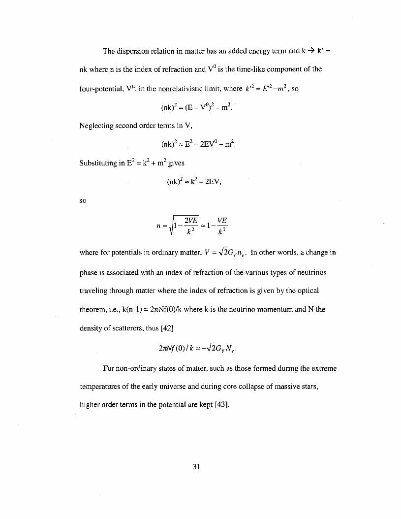
The dispersion relation in matter has an added energy term and k 7 k' =

nk where n is the index of refraction and VO is the time-like component of the

four-potential, V''\ in the nonrelativistic limit, where k'2 =£,2 _m2, so

Neglecting second order terms in V,

Substituting in E2=k2+ m2gives

(nk)2 "" k2- 2EV,

so

where for potentials in ordinary matter, V =.J2GF ne • In other words, a change in

phase is associated with an index of refraction of the various types of neutrinos

traveling through matter where the index of refraction is given by the optical

theorem, i.e., ken-I) = 2nNf(O)/k where k is the neutrino momentum and N the

density of scatterers, thus [42]

For non-ordinary states of matter, such as those formed during the extreme

temperatures of the early universe and during core collapse of massive stars,

higher order terms in the potential are kept [43].

31

The difference in the refractive index in the case of the electron neutrino

and the other flavors is ~n = 7.6 x 10-19 ( P 3)( E ). Although this is100g/em lOMeV

indeed a small value, it leads to significant differences for those in vacuum if the

neutrinos have non-zero masses [44].

By bringing together the spatial phase shift for the induced refraction of

the neutrinos in the solar medium with the temporal phase shift from the mass

matrix in vacuum, Wolfenstein was able to describe the change in vacuum

oscillations in matter caused by the differences in the effective masses and indices

of refraction of the neutrino interactions with the ambient solar interior through

charged and neutral current electroweak interactions [45].

2.4 The Neutrino Propagation Equation in Matter

The Klein-Gordon (KG) equation is a relativistic propagation equation for

spinless particles with mass and can be represented in the form

Since the weak interaction only couples to the left-handed components of the

neutrino field, the spin structure from the wave equation may be eliminated so

32

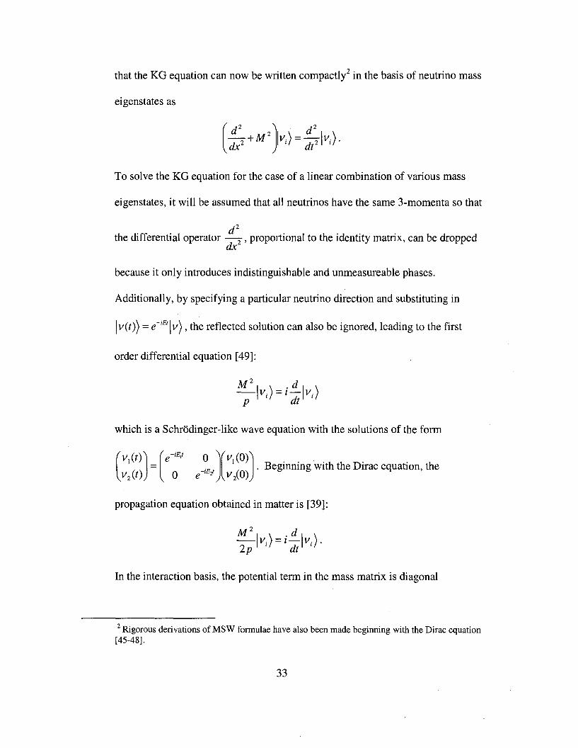
that the KG equation can now be written compactli in the basis of neutrino mass

eigenstates as

To solve the KG equation for the case of a linear combination of various mass

eigenstates, it will be assumed that all neutrinos have the same 3-momenta so that

the differential operator d2

2 , proportional to the identity matrix, can be droppeddx

because it only introduces indistinguishable and unmeasureable phases.

Additionally, by specifying a particular neutrino direction and substituting in

Iv(t») =e-iE1Iv) , the reflected solution can also be ignored, leading to the first

order differential equation [49]:

which is a Schrodinger-like wave equation with the solutions of the form

° ](V1(O)] B " . h h D' . h'E • egmnmg WIt t e Irac equatIOn, t ee-121 via)

propagation equation obtained in matter is [39]:

In the interaction basis, the potential term in the mass matrix is diagonal

2 Rigorous derivations of MSW formulae have also been made beginning with the Dirac equation[45-48].

33

which becomes (Appendix E),

where 2.fiOFneEv ' This evolution equation holds for the propagation of either

Dirac or Majorana particles where the mass matrix in the case of constant density

is determined by adding an induced electron neutrino mass term (A = .fiOFneE)

to the mass squared matrix in vacuum, i.e., M 2-7 M 2 + A (Appendices D&E),

so

i~(:eJ=_1(- ~:OS28+ A ; sin 28J(:eJ.dx f-l 2E -sm28 -cos28 f-l

2 2

The matter-mixing angle, which controls the oscillation probability, is

obtained from the trigonometric relation

tan 28M

= sin 28M = 2(HM )12 = li sin 28cos 28M (H M ) 22 - (H M ) 11 li cos 28 - A

It can also be recast into an equivalent, but more telling form

. 2 28 _ li2

sin 2 28sm M - ( )2 .

licos 28 - A +li2 sin 2 28

This equation is of the form of a resonance equation, such as that of Breit-Wigner,

where the resonance half width is rt2 = lisin28. This equation describing the

34

mixing angle in matter shows the degree of mixing between the linear

combination of flavor states upon creation, while propagating through the

resonance region and as it emerges from the solar surface. (See Figure 31.)

As the mass eigenstates propagate, they each acquire a different phase;

yet, they are not the states that are produced or detected through the weak

interaction. Instead, the physical quantities one observes during neutrino

production and detection are the flavor eigenstates because of the weak

interaction processes of neutrino creation and destruction. It is the

parametrization in terms of the rotation (mixing) matrix that allows the neutrino

mass eigenstate solutions to be described in terms of the neutrinos that are

produced and detected. However, it is generally believed that it is not Ve and vI!

which propagate in space but, instead, VI and V2 [50].

35

2.5 Propagation Equations for Homogeneous Densities

In the case of vacuum oscillations, the evolution equation can be written as

. d (VI (t») (VI (t»)1 dt V

2(t) =H v

2(t)

where H is diagonal in the basis of mass eigenstates, i.e., H = ( ~' 0) andE2

2

Ek :::: p + mk represents the energy eigenvalues in vacuum. In the flavor basis the2p

equation is

I + m l2 + m~ m~ - ml

2(-COS28

where H =UHU =P + + ---=---=-4p 4p sin 28

and the mixing angle is given by2H'

tan 28 = 12

H'22-H 'l1

sin 28) (Appendix D)cos 28

The evolution equation for neutrinos propagating in matter modifies the

above equations, so that

where

-~cos28+J2GFne4p

~sin284p

~sin284p8

-cos284p

36

and H M =V =.[iGFne in direct correspondence with the equation for vacuum

oscillations. In other words, under a unitary transformation using the matrix U

which connects the mass and flavor eigenstates, the evolution equation takes the

above form. The effective mixing angle in matter, 8M, is now given by

2(H ) ~sin28tan 28 - M 12 =-----M-

(HM )22 - (HM)l1 ~cos28- A

where A =2.[iGFneP and ~ =m; - ~2 , again, in direct analogy with the

equation for the case of vacuum oscillations. The effective mixing angle is a

function of the electron density and A is related to the induced effective mass

, ~cos28when resonance occurs as A = ~cos28, or ne = J2 since

2 2GFP

Expressing the corresponding mass eigenstates in matter for the case of

constant density in terms of their respective flavor eigenstates can be obtained

through the analogy with the transformation equation for vacuum oscillations

where the equations for the case of homogeneous density are identical to the case

of vacuum oscillations except now VI ~ (vM )1 and 8~8M. Thus -- with the

appropriate modifications -- the behavior of electrons propagating in

homogeneous density matter is the same as in vacuum, i.e., no resonance

modifications occur for neutrinos traveling through media with constant density.

37

2.6 Neutrino Flavor Conversion in Media withNonhomogeneous Densities: The MSW Effece

One of the important things to keep in mind when dealing with neutrinos

propagating in media with nonhomogenous densities is that the mass eigenstates

are no longer eigenstates of the Hamiltonian, so that instantaneous solutions in the

adiabatic approximation are sought. For convenience we will use a more

abbreviated notation, where IfF! ~ (~:), so the flavor evolotion equation is now

. d 1 M 2l-lf/ =- If/.dx f 2£ f

O2J'the interaction evolution equation becomes

M2

where UM = UM(X), so (Appendix E):

where the second term on the right hand side accounts for the inhomogeneous

density. In the case of homogeneous density the differential term does not appear.

In the above equation, UM is the mixing matrix in matter

1 This section is noticeably indebted to T.K. Kuo and 1. Pantaleone, "Neutrino oscillations inmatter," Rev. Mod. Phys. 61 (1989) 937.

38

(

COS 8MU =M . 8sm M

and U~ its Hermitian conjugate. The off diagonal terms in the matrix of the

mass eigenstate evolution equation are what cause the states Ivl ) and Iv2 ) to mix,

where the interaction should be thought of in terms of instantaneous mass

eigenstates:

The adiabatic condition for the phenomena of matter enhanced oscillations

can be obtained by starting with the adiabatic inequality -- 0E8t» n-- in terms

of the energy gap between the levels, 8E, and the time of transition where the

neutrino is in the level crossing region, 8t [ref. 44, p. 106]. The energy gap can be

obtained using the relativistic approximation to the energy difference equation

m 2 _m2 11where I1E::::: 2 I and, so OE - -·-sin 28. The density gradient is

2p 2E

.!!- (In ne ) =~ dne ,so the inverse of the transition time between the gap can bedr ne dr

written (as r ~ t and d - 8) as ~ =~ dne~ - (~ dne)~ where A =I1cos288t ne dx &Ie ne dx M.

at resonance so 8A -l1sin28 (the width of the resonance). Since OE =~sin 282E

39

d e (1 dne J-1

8sin 28 h ' h' I' +' han at = --- ----, t en usmg t e mequa tty lor t e energy gapne dx 8cos28

8£& »1 (since tz =1), we obtain

8 . 28( 1 dne J-1

8sin 28 1-sm --- » .2E ne dx 8cos28

The adiabatic condition at resonance is often written in the form (y» 1) where

8sin 2 28y=---.,.....-----,-

2Ecos28~dne

n dxe res

therefore, leading to a negligible hopping probability, since

and for large y, Phop -7 0

The formula for the electron neutrino survival probability is given as [51]

where PLZS is the Landau-Zener-Sttickelberg transition probability and 8~ is the

mixing angle in matter at the point of production. When the above adiabatic

condition holds (i.e., y» 1), then the transition probability, the probability for a

neutrino on one of the trajectories to jump to the other trajectory in the level

crossing diagram, becomes negligible, soP(ve ~ vJ =~(l + cos 28~ cos 28) ,

40

independent of whether the neutrino passes through the resonance or not [ref. 27,

p.950].

Whflt this means in terms of the allowed parameter space for neutrino

oscillations (~ vs. sin2 28) in the Sun, is that the diagonal, nonadiabatic region can

be eliminated. (See Figure 5.) Recent results from KamLAND in combination

with solar neutrino data, have found that the small mixing angle (SMA) solution

and the LOW ~m2 region can also be excluded leaving the large mixing angle

(LMA) region on the MSW plot as the leading solution to the solar neutrino

problem. From analyses of solar, atmospheric and reactor neutrino experiments

the following neutrino oscillation parameters for 10' allowed ranges are found [3]

tan 2 8 =0 41+0.0812 • -0.07

sin 2 2823 > 0.92

tan813 < 0.16

As the effective mixing angle in matter determines the oscillation

probability, P =P(8M), the mixing angle in matter, 8M , in tum, depends on the

electron number density and energy at a given point, i.e., 8M =8M (nix),E).

Therefore, the propagation equation describing mass eigenstates in matter

represents the Hamiltonian changing adiabatically from point to point. In this

situation, the vJ.L fraction of the propagating wave packet has sufficient time to

41

build up as long as the resonance condition is met, Le., cSt =cSx »Lose. At

resonance, the hopping probability - the probability for one eigenstate to jump

abruptly to another eigenstate - for the solar interior is negligible since the density

varies gradually enough to fulfill the adiabatic condition. In other words, if the

density term varies sufficiently slowly so that the oscillation length is of the order

of one wavelength in matter, then the off diagonal terms in the mass squared

matrix may be ignored and IVI) and Iv2) become instantaneous mass eigenstates

of the Hamiltonian.

In the case of a medium with an inhomogeneous density profile, 8M

depends on the gradient of the electron number density as well as the neutrino

energy (in the sin2 8M equation) [53]. The propagation equation in the mass

eigenstate basis in matter can be written (Appendix E) as

d8M 1 Llsin 28 dAwhere - =- ( )2 ( )2 [ref. 27, p. 949], or

dx 2 A - Ll cos 28 + Ll sin 28 dx

more explicitly in terms of electron number density [49]

42

In the case where there is no density variation (Le., where the electron number

density is constant), then d8M = dne =0 and the system of equations reduces todx dx

that of the stationary state analogous to the case of vacuum oscillation where

The radial density inhomogeneity variation in the solar core gives rise to

the possibility of resonance conversion when the adiabaticity condition is

fulfilled, i.e., 181« 1m; - m;l. Under these circumstances the Hamiltonian can be

defined at a given point, i.e., the matter eigenstates pass through the medium with

a constant relative mixture of Ve and vJ..l at a given point. The oscillation length at

resonance is L = 47tE which is the scale on which the interference occurs.res 8sin 28

In this case, the vJ..l fraction of the propagating wave packet in Ve has sufficient

time to build up (i.e., 8t =ox), or distance over which to match the slowly

changing density as long as the resonance condition, Ox » 4es, is satisfied.

When the traveling electron neutrino enters the resonance region of the Sun

(-Ro/5), the flavor of the complete state, Le., Vz, matches the changing density, so

that a non-oscillatory flavor transition takes place because of the mixing between

the mass eigenstates, VI and Vz [54].

At the surface of the Sun, the electron survival probability is

approximately equal to sinze which gives it its characteristic non-oscillatory

43

transition probability. Due to the fact that solar neutrinos have a relatively short

coherence lengths, - 10-6 cm, having been created from rapidly oscillating nuclei

in the hot solar core [55], the neutrino mass eigenstates will be incoherent so

phase information will be lost, leading to a classical probability. In this case, the

oscillatory term will be averaged out, so

Thus the neutrinos travel from the core of the Sun, pass through the narrow region

in which the effective mass enhancement occurs (as some mixture of Ve and va)

and exit from the solar surface and travel to the Earth relatively unchanged from

the state acquired upon leaving the solar surface [56].

Depending on the initial energy and the point of neutrino origin there are

three neutrino energy regimes: 1) below 2 MeV (i.e., the energy region with

which most of the neutrinos are formed in the pp reaction in the Sun), where there

are only small matter corrections to the vacuum oscillations; 2) between 2 MeV

and 10 MeV, where there is a noticeable non-oscillation contribution in addition

to the oscillation effect; and 3) above 10 MeV, where the non-oscillatory

adiabatic effect dominates (along with some small oscillation effects). The

measured average probability is somewhat higher than that expected from a pure

sin2enon-oscillatory term alone which may be attributed to the effects of

44

hypothetical sterile neutrinos,2 whose overall effect is one of a completely non-

oscillatory matter effect for certain values of the mass difference [ref. 54, p.16].

When the adiabatic condition is valid, the mass eigenstates can be

considered instantaneous eigenstates of the Hamiltonian, so that the linear

describes the state of the neutrino at a given point of constant electron number

density. In conjunction with this fact, the level crossing diagram and the mixing

angle in matter versus the electron number density diagram portray the behavior

of the neutrinos when they are created in the solar core, propagate through the

critical density region (provided that they have a sufficient energy), and exit from

the solar surface. (See Figures 3 and 32.}

When an electron neutrino is first created in the Sun, it finds itself in a

region where the electron density number is significantly greater than at

resonance, i.e., ne »n;es. From the diagram of the matter mixing angle versus

density, it can be seen (Figure 32) that the matter mixing angle is at its greatest

value (8M ::::: n ), and the electron neutrino is primarily in the high mass2

eigenstate, i.e., !vz)::::: Ive ). At this point the mixing length in matter is given (in

analogy with that in vacuum) as LM = 4nE (where /).. M =m~ - mlz) which is

/)..M

much less than that in vacuum -- making the MSW effect physically significant.

2 Alternatively, the larger than expected survival probabilities may be due to density fluctuationsin the solar core [57].

45

When the neutrino enters the region where ne =n;es , the mixing angle in

matter is such that maximal mixing occurs, i.e., eM =n, where equal amounts of4

the two flavors (in the two flavor model) make up the mass eigenstate of the

propagating neutrino.

Finally, as the neutrino reaches the solar surface, where ne «n;es , the

. . 1 . ... . l' e 0 h L 4nE hmlXmg ang e m matter IS at ItS mmlmum va ue, I.e., M = were =--, t e~

same as that in vacuum and Iv2) =IVa) .

If an interaction does occur between Ve and Va (i.e., e "# 0), there is no level

crossing and the levels repel each other. The nature of the level crossing can be

understood in terms of a state system where the energy levels are a function of

some parameter, such as an external magnetic field which changes slowly.3 When

A =~cos28 =2.J2GFneEcrit ' the distance between the levels is a minimum. If a

neutrino is created in the Sun with E > Eerit (or P > Perit) then the Ve appears on the

upper right hand comer of the level crossing diagram. (See Figure 3.) As the

neutrino passes through the Sun toward the surface, both the electron density and

the magnitude of the resonance parameter, A, decrease. If this decrease takes

place slowly enough such that the adiabatic criterion holds, the neutrino's

trajectory corresponds to the upper curve where the neutrino is made up of a

linear combination of flavor eigenstates. Thus, an electron neutrino that is created

3 The crossing point can be viewed as a diabolical point whose collective point always tries to goas far as possible from the point of degeneracy, as a charged particle in a magnetic monopole [58].

46

in the high-density region of the solar interior will arrive at the solar surface as a

higher mass eigenstate neutrino, i.e., Iv2 ) with a reasonably high probability of

being in a non-electron neutrino momentum state, i.e.,Iva)'

The above argument follows from the adiabatic theorem which says that if

the newly-created neutrino begins on either of the two trajectories, then it will

continue on that trajectory as long as the density changes adiabatically; otherwise

a level crossing will occur with the probability given by Phop . Because the

neutrino mass matrix is a function of the solar density, the mechanism whereby

the density effects the neutrino mass is due to the differences in the nature of

scattering that the various neutrinos experiences as they travel through the

resonance region. If the density that the neutrinos are passing through is constant,

then the flavor eigenstates in terms of the mass eigenstates may be written

explicitly as

where (}M is defined through the equation tan 2(}M = sin~ . When

2() 2 2GF ne Pcos + -2 -2

m2 -m1

ne = 0, then 8M = 8 and the flavor eigenstates are the same as the mass eigenstates.

If m2 > mt and the density is very large and ne ~ 00, then lim (}M (ne ) -7 1l andne~OO 2 .

47

so every neutrino produced as ve (at a density greater than the critical density) will

be primarily in the heavier mass eigenstate, i.e., Ive(ne)) =:: Iv2 (ne)) where an

equality holds when ne ~ 00.

The critical resonant solar neutrino energy is given by [ref. 59, p. 263]

(11m

2 JEcrit =6.6cos8 10-4 eV 2 MeV

and the corresponding critical density, where 8M (n;rit) = 7r , is [ref. 59, p. 262]4

In the case of the Sun (using the combined results from KamLAND and the solar

neutrino data) the resonant energy is about 4 MeV with a critical density between

90 glcm3 (O.IRo) and 10 glcm3(- O.3Ro). Thus, the neutrinos emitted in the

boron-8 (and hep) reaction(s) will have sufficient energy to pass through the

resonant region and convert to one of the other generations on its way out of the

Sun. The extent of flavor conversion also depends, however, on the distance

between where the neutrino originates and where the resonance takes place, so

that the point where the neutrino is produced (in terms of electron density)

determines its initial degree of mixing [ref. 54, p.12].

48

Summary

Neutrino propagation in matter is governed by the matter wave equation

which can be obtained from the Klein-Gordon equation. (Alternatively, one can

use the Dirac equation via field theory.) The neutrino mixing angle in vacuum is

similar to the Cabibbo angle for the analogous system of quarks where the quark

mixing matrix, known as the Cabibbo-Kobayashi-Maskawa (CKM) matrix, arises

because the quark mass eigenstates are not identical to their weak interaction

eigenstates. Since there are no fundamental symmetries to prevent the neutrinos

from having mass, the existence of massive neutrinos does not violate any known

conservation laws, i.e., the existence of massive neutrinos only requires a minimal

extension of the SM.

When a neutrino is produced via the weak interaction it is in an interaction

eigenstate and afterwards it propagates through the medium in a superposition of

mass eigenstates. Since the flavor and mass eigenstates are not in general the

same, neutrino flavor will not be conserved during propagation. Unlike the case

of quarks, the difference between the neutrino masses (as given by the Maki­

Nakagawa-Sakata (MNS) matrix) is sufficiently small that the flavor can

noticeably change over macroscopic scales (i.e., - 180 km, KamLAND (2003)).

The effects of neutrino propagation in homogeneous density matter was

initially described in terms of an optical analogy, where neutrinos propagating

through matter forward scatter from off of the background matter inducing indices

49

of refraction for Ve, vI! and V't whose magnitude depends upon the flavor. Under

these circumstances, Ve and vJl will have different indices because the ambient

background contains unequal amounts of electrons and muons (essentially zero),

so that if the neutrinos are massive then the flavors will mix in accordance with

the mass matrix as they pass through the solar core whereas vJl and V't will have

the same values for n. Because the index of refraction acquired by the electron

neutrino behaves in a way that is similar to an additional mass term, the flavor

dependent indices can greatly affect the degree of mixing of the mass eigenstates

during neutrino propagation. This disparity between the index of refraction for Ve

and vJl (or v't) can lead to resonant enhancement or suppression of Ve, if the

neutrino has sufficient energy as it propagates through the resonance region of the

Sun.

The time evolution of the state vector in matter in the flavor basis is

governed by the equation

i.!!-(Ve(t)J =_l_(m; cos2

B+ m~ sin2

B+ A ~sin BcosB J(Ve(t)Jdt va(t) 2£ ~sinBcosB m;sin2B+m~cos2B va(t)

where the eigenvalues of the squared masses of the matrix equation for Ve and Va

are (Appendix C)

and the equation for the mixing angle in matter is

50

• 2 28 _ 1::.2

sin2

28sm M - ( )2 2'

I::. cos 28- A +1::.2 sin 28

Transforming the neutrino flavor time evolution equation into one in terms of the

mass eigenstates, (vM)[ and (vM)2 ' through a unitary transformation using

(

COS 8MU =M . 8sm M

puts the equation into a form that more clearly shows the nature of the conversion

in matter when the neutrinos propagate in a medium where the density changes

. I::. sin 28 EdAl -

-2 -2 dxm2 -m[If/M

In the adiabatic approximation, the density changes sufficiently slowly so

that the matrix in the above equation will be nearly diagonal, i.e., there will be no

mixing between the two (2) diagonal eigenstates. Provided that the off-diagonal

terms are small compared to .!. (iii; - ~2 ), the adiabatic approximation will be2

satisfied.

The amounts of Ve and Va change relative to one another, in the adiabatic

approximation. Therefore, in analogy with the vacuum oscillation equation, the

electron survival probability of an electron neutrino in matter is now given by

51

where LM = ( 4')zE is the oscillation wavelength in matterA - ~ cos 28 +~2 sin 2 28

and L is the distance from the neutrinos production point to the location of the

detector. When the neutrino passes through the critical density region, (i.e., A =

~cos28), there is resonant modification such that the resonance oscillation

wavelength is 4es = 41tE/~sin28 as long as m2 > mI.

In the level-crossing diagram (Figure 3), the straight horizontal and

diagonal lines represent the expectation values for the masses, ~2 and m~ , for the

states Ve and vI! in vacuum where the energy and mass eigenvalues for neutrinos

-2

in m~tter are given by Ek ::= P + mk and the mass eigenvalues in matter, iii;2'2p .

The behavior of ~2 and iii~ as functions of A are shown, where the ordinate is in

terms of the mass matter eigenstates and the abscissa can be taken in terms of

increasing density, p, or the resonance parameter, A. When A» ~cos28, 8M ~

1tI2 and so the heavier eigenstate V2 is almost purely Ve while the lighter eigenstate

VI is almost entirely vI!' When A =0 (i.e., for very small mixing angles) as in

vacuum, the lighter eigenstate VI is almost completely Ve while the heavier

eigenstate V2 is nearly all Va. From the above survival probability equation, it can

be seen that the nature of neutrino propagation in matter depends upon the

vacuum oscillation eigenvalues, ~2 and m; ,as well as the electron number

density and neutrino energy.

52

In the case of the Sun, the varying density between the center and the

surface causes exiting electron neutrinos to convert into other flavors because the

nature of the low-energy weak interaction is influenced by the changing effective

mass of the neutrinos in matter as the matter mass eigenstates endeavor to match

the changing density as the neutrinos propagate outward from the point of their

origin. The flavor conversion that takes place in the solar interior is due to the

change in mixing and not the change in relative phase, as in the case of vacuum

oscillations.

The large mixing angle (LMA) MSW solution offers a satisfying

explanation for the solar neutrino problem. In the case of varying density, the

adiabatic flavor conversion gradually transforms Ve into a vI! (or v1) while passing

through the resonance layer. Under these circumstances, the mass eigenstates

become instantaneous eigenstates of the Hamiltonian so that a change in mixing

takes place as the neutrino passes through the solar interior causing a certain

fraction of electron neutrinos to convert into non-electron neutrino flavors, i.e.,

ve ~ va' In the adiabatic approximation, the neutrino leaves the surface of the

Sun in a vacuum mass eigenstate so that there are no further oscillations enroute

to the Earth. Recent studies, however, have found a detectable transformation of

va ~ ve as the converted neutrinos regenerate when they pass through the

Earth's interior, known as the day-night effect [130,131].

53

3.0 Partial Degeneracy in the Solar Core

The electron degeneracy pressure and number density in the solar interior

can be obtained from the equations

5/2 (2 )Pe =CkT 3" F312 (1])

where C = 4~ (2mkYI2. The problem, however, is that since the electronh

degeneracy parameter, 11, is a function of the pressure and the temperature, i.e., 11

=11(P ,T), the equations must be solved through iteration using the two equations

[ref. 60, p. 27]:

and

(Y Z J 1 =f (dUrfJP-pRT X +-+- =- pne(p) - P4 Az 3 0 dp

where f3 = 1 - aT4/3 P is also a function of temperature and pressure, f3 = f3(P, T).

Another way of saying this is that these interrelated equations must be solved

simultaneously with respect to a particular solar model. Here, the standard solar

models (SSMs) developed by J. Christensen Dalsgaard (JCD1987)1 and J.N.

I http://www.helios.tllc.gong.noao.edu/teams/models/gong-www.14b.d.18.html (MNRAS 199(1982) 735).

54

Bahcall and M.H. Pinsonneault (BP2000)2 will be used to obtain the needed

density profiles as functions of the pressure and temperature, i.e., p =p (P, T). By

using the relation between the electron degeneracy parameter and the solar

pressure, the percent change in the electron degeneracy pressure could be arrive at

as a function of the solar radius with the help of these SSMs. The electron

degeneracy overlaps with the same region where the MSW effect occurs in the

Sun (0.1 Ro - 0.3 Ro) for various energy neutrinos. (See Figure 9.) In this study,

the total percent change in the electron number density at the solar center was

found using the ratio between the FD integrals F312 (17) and F1I2 (1]) [ref. 17, p.

97]. The maximum value of the partial electron degeneracy at the solar core

using this technique was found to be around 1.8%.

The differences in the maximum value for the electron degeneracy

between calculated values from Stix (-1.7% (Figure 6» and those performed here

(Figure 9) may be due to the fact that values for 11 are model dependent, i.e., 11 =

l1(P ,T), so the differences in the partial degeneracy of the solar interior requires

close examination when detailed comparisons between standard solar models

need to be made, because a linear approximation between various FD integrals

was used instead of calculating them individually for each solar shell.

2 http://www.sns.ias.edul-jnb/SNdataJExporUBP2000lbp2000stdmodel.dat (Astrophys. J. 555,(2001) 990).

55

The linear approximation used for the solar electron number density

(fermi3.f) introduced some error into the electron degeneracy profile that can only

be corrected by performing detailed calculations for each shell of the solar model

being considered. This may be accomplished in the future by FORTRAN

programs available in [22,23]. Neither of these programs, which calculate FD

integrals, could be easily incorporated into the program which calculated the

integrated neutrino conversion probabilities written by D. Casper [62], because

the way the I/O subroutines were structured may have entailed significant changes

to the organization and possibly the integrity of the algorithms. In the future an

entirely new procedure should be written that calls each of the routines in a clear

and consistent manner while continuously checking for errors and any possible

instabilities in the calculations during run time. The best way, however, to obtain

the most accurate electron degeneracy profile is through the implementation of a

routine during the run-time calculations of a given SSM.

In light of these considerations, the question which this paper raises is how

much does the electron degeneracy pressure influence the resonant matter

oscillations of the electron neutrinos exiting the solar core, i.e., what is the percent

difference in the total electron survival probability after passing through the

critical density regime with and without electron degeneracy? Even though the

influence of electron degeneracy on the MSW effect in the Sun amounts to only a

small correction, the importance of such effects may become increasingly relevant

as more precise neutrino experiments and solar model calculations are conducted.

56

For instance, the relativistic effects of solar electron degeneracy [63] and the

possibility of density fluctuations in the solar core [57] are now being studied

because the high degree of precision attained by neutrino experiments and SSMs

allow for such meticulous scrutiny. More detailed calculations that include solar

opacity calculations also incorporate the effects of partial electron degeneracy

[77].

In the case of high-density matter, accurate calculations of the survival

probability of electron neutrinos may shed significantly new information on the

neutrino emitting processes associated with core collapse of massive stars during

supernova (SN) explosions as well as physical properties of neutrinos. For

example, in calculating the electron neutrino survival probabilities for the thermal

stage of core collapse, accurate values of the solar neutrino oscillation parameters,

I1m;z and BIz' are needed. The importance of the MSW effect in SN explosions

arises because, in addition to the neutrino emitting thermonuclear processes

taking place in the Sun, SNe are believed to be the only other naturally occurring

phenomena where neutrinos can be measured -- assuming that the core collapse

occurs within 50 kpc. Through such astrophysical events, such as SN 1987A, a

determination of (or, strong bounds on) the absolute masses of the neutrinos

becomes possible because of the great distances between the neutrino source and

the detectors allowing for incredibly small mass differences to be determined

[64].

57

A verifiable determination of the absolute magnitude of the neutrino

masses is a question of great theoretical interest for physics, astrophysics and

cosmology. Inversely, through helioseismologicalobservations, a more accurate

density profile of the Sun may be achieved. At present, a good deal of the

calculations being done on SN neutrino fluxes treat the case when the degeneracy

parameter 11 is set to zero. Investigating the effects of electron degeneracy on SN

neutrino emission and flavor conversion may prove to be worthwhile because of

the fact that the theory of partial degeneracy is well understood, and, additionally

it is conceivable that detailed information of the effects of electron degeneracy on

the MSW effect in the case of the Sun may offer some valuable information in the

case of SNe neutrinos.

During the later stages of stellar evolution (or during supernova

explosions), the kinetic energy of the electrons in the central regions of the

matured Sun will become large enough (on the order of billions of years when it

becomes a white dwarf star) so that the magnitude of the thermal energies will

approach the rest mass of the electron, i.e., kT - mec2 and ve - c. Integrating

over the momentum space gives relativistic expression for the electron number

density

where the Fermi distribution function is given by f = (1 )/kT [65].e 1+ e e-p,

58

4.0 Neutrino-Emitting Thermonuclear Reactions

The process of nuclear energy generation taking place in the Sun's core

produces radiant energy in the form of photons which provide a radiation pressure

that counteracts the contracting gravitational force. Throughout the Sun's lifetime

these same nuclear reaction processes bring about chemical transformations that

change the Sun's structure and subsequent evolution. The energy generation of

the present Sun, however, is sustained by burning hydrogen through the proton-

proton chain and theCNO cycle where any variations in composition, temperature

and density affect the relative frequency of the various pp branches. This is one of

the principle hypotheses underlying standard solar models [66].

The first step, in the transmutation of hydrogen into helium via the pp

chain, occurs when two proton nuclei penetrate the electrostatic Coulomb barrier

and achieve nuclear fusion. The primary sequence of the pp chain, the Im1

branch, is shown in the table below.

h [59 60]Ibd fT bl 1 N Ia e uc ear reactIOn ata or PP ranc ,Nuclear reaction Qth (MeV) Qv (MeV) Time

P+ p~d+e++ve 1.192 0.250 1.4 x lOw yrs

p + d ~ 3He +Y 5.494 ----- 6sJHe + jHe~4He+2p 12.860 ----- 10° yrs

Because the first two steps must occur twice, in order for the final step in the ppl

branch to complete, the total energy liberated in the formation of a helium nucleus

is 26.732 MeV where Qth is the thermal energy delivered to the interior of the Sun

59

and Qv is the average energy lost to the Sun through neutrino emission (0.5 MeV).

In the formation of the deuterium nucleus, along with the simultaneous production

of a positron and electron neutrino, there is a sufficiently low nuclear reaction

conversion probability so the p + P reaction ultimately determines the overall rate

of solar energy generation. This is due to the fact that the reaction takes place

through the weak interaction with its characteristically small interaction cross-

section ((j oc G;). The extremely long time that it takes to create deuterium

explains the gradualness with which the Sun bums hydrogen.

In the following table for the pp2 branch of the proton-proton chain, the

neutrino emission line for the formation of lithium-7 is split because the final

product may be in either an excited state or its ground state, so that emitted

electron neutrinos appears as two distinct lines. Another important emission line

that appears in the proton-proton chain (not shown in the table) takes place

through the three particle reaction p + p + eO ~ d + Ve. However, this reaction's

rate of occurrence is only 14 % that of the p + p ~ d + e+ + Ve reaction [ref. 60, p.

48] whose average reaction time is 1012 years [ref. 60, p. 67].

h [59 60]2bd t fT bl 2 N Ia e uc ear reaction a a or pp. ranc ,Nuclear reaction Qth (MeV) Qv (MeV) Time3He + 4He~7Be + y 1.586 ----- lOt> yrs7Be + e- ~ 7Li + Ve 0.049 0.862 (0.384) 36 dys'Li + p ~ 2 4He 17.348 ----- 5 min

60

The pp3 branch begins with the same first step as the pp2 branch, i.e., the

formation of beryllium-7, but then proceeds via proton capture instead of electron

capture in the following sequence:

h 5 63bd f hT bl 3a e : Nuc ear reactIOn ata or t e PP: ranc [ 9, 0]Nuclear reaction Qth (MeV) Qv (MeV) Time

7Be +P ~ 8B +Y 0.137 ----- 100 yrs8B ~ 8Be* + e+ + Ve 7.9 7.2 0.8 s1SBe ~ 2 4He 2.995 ----- 10=TO s

The interpolated reaction rate for the pp chain is given by Epp oc pX2 T64 [ref. 67,

p. 83] where p is the mass density, X is the mass abundance of hydrogen, and T6

is the absolute temperature in units Tn = T/lOn K. According to the SSM, the

eNO, or carbon, cycle accounts for only about 1 - 2% of the energy generation in

the Sun:

I [59 60 66]br d t f h

Marks begmnmg of secondary reactIOn sequence WIth a 1/10 occurrence ratio

a e uc ear reac Ion a a or t e car on cyc e , ,Nuclear reaction Qth (MeV) Qv (MeV) Time12e + P ~ l3N +Y 1.943 ----- 1.3 x 107 yrs13N~l3e+~+e++ Ve 1.514 0.7067 7 minl3e + p ~ 14N + Y 7.551 ----- 2.7 x 1O() yrs

14N + P ~ 150 + Y 7.297 ----- 3.2 x 1cr yrs150 ~ 15N + e+ + Ve 1.754 1.00 82 sl:lN + p~ 12e + 4He 4.966 ----- 1.1 x 105 yrs160 + P ~ 17F + Y 0.600 ----- -----

17F ~ 170 + e+ + Ve 1.763 0.9994 -----lIO + P~ 14N + 4He 1.191 ----- -----

a

T bl 4 N

61

As can be seen from the primary reaction sequence, four protons are converted

into one helium nucleus with a total energy generation, Q =Qth + Qv=26.732 MeV

which is the same as that produced by the proton-proton chain. The bottleneck in

the carbon cycle is the 14N + P~ 150 + Y step since the average time required

for the transmutation of nitrogen-I4 into oxygen-I5 is over 300 million years.

The interpolated energy generation rate for the CNO cycle written as

fCNO oc pXXcNT619 [ref. 67, p. 83] where XCN as the sum of Xc and XNis used

because the mass fraction for XCN is constant while the individual carbon and

nitrogen fractions change [ref. 67. p. 81]. The pp chain dominates at temperatures

less than T = 1.5 X 107 K whereas at higher temperatures the CNO cycle takes

over and pp chain becomes unimportant since the reaction rate for the pp chain

goes as fpp oc T64 while that for the carbon cycle is fCNO oc T6

19. The Sun,

therefore, only generates about 1.6 % of its energy from the CNO cycle since Tc

= 1.57 X 107 K while the remaining 98.4% is created through the reaction

sequences associated with the proton-proton chain.

Variations in the temperature and densities in the interior of the Sun lead

to surprising differences in abundances for a range of depths, even for a single

reaction. 3He consumes itself at the Sun's core with a mean lifetime of about 106

years, yet it accumulates significantly at a depth of about RoI4, or 2 x 108 m.

Meanwhile, 4He is steadily accumulating in the central region of the Sun. For a

number of nuclear species, such as 2H, 7Be, 7Li, 8B and 8Be*, relatively short

lifetimes cause them to come into rapid equilibrium. The densities of the various

62

species do change but at sufficiently slow rates so that their abundances follow

other less rapidly changing species. Looking solely at the neutrino producing

reaction steps, we find:

[5960 68]t .T bl 5 R f d t fa e eac IOn a a or neu nno processes , ,Nuclear reaction Chain/branch!cycle Qv (MeV)a Qmax (MeV)IH(p, e+ Ve)2H pp1,pp2,pp3 0.250 0.4207Be(e-, Ve)7Li pp2 0.813 0.862(0.384)8B(e+ve)8Be* pp3 7.2 14.0613N(e+Ve)13C CNO 0.7067 1.199150 (e+ve/

5N CNO 1.00 1.73217F(e+ve)170 b CNO 0.9994 1.740IH(p e-, Ve)2H pp1 1.442 1.4423He(p, e+ve)4He pp1 -10 18.773a Qv is the average neutrino energy bThis reaction rate is negligible: 1/103

The total average energy yield per cycle in the Sun (less that due to neutrino

losses) is about 25 MeV and the total solar luminosity Lo =3.85 X 1026 W, so the

number of neutrinos produced from the hydrogen burning proton-proton chain

and the carbon cycle is Nv = Lo/<E> =(3.85 x 1026 J/s)/(4.01 X 10-12 J) =9.60 x

1037 vis. However, since two neutrinos are created for every 25 MeV produced,

63

the total number of neutrinos emitted is Ny = 1.92 X 1038 vis. The total flux of

neutrinos reaching the Earth per second per square meter is given by f =Ny/cr, so

f =Ny /4nR2 =(1.92 x 1038 vis) 14n(1.496 x 1011 m)2 =6.83 x 1014 v/m2/s.

There are also neutrinos which are formed in the rare three particle pep

reaction, p + p + e- -7 d + Ve and the highest energy neutrino emitting hep

process, 3He + p -7 4He + e+ + Ve which must also be taken into account. From

the above table of neutrino producing reactions, the neutrinos emitted with

electrons have continuous energy distributions described by Fermi's theory of

beta decay [69] while those such as the pep reaction and 7Be(e-,ve)7Li exhibit

discrete neutrino line emission spectra.

4.1 Nuclear Reaction Rates

The equilibrium reaction rate formulae for Epp and ECNO are actually not

useful for obtaining the solar neutrino spectrum; instead, all the nuclear reaction

rates for each individual reaction in the pp chain and the carbon cycle must be

used. To correctly derive the formula for the nuclear reaction rates, one should

realize that the elementary reaction process describes the collision between two

completely ionized nuclei, where the number of interactions that take place per

cubic centimeter per second can be represented as [ref. 67, p. 77]:

64

=

r = f N 1N2Vq(V)Pp(v)PND(T,v)dvo

where the number of colliding nuclei, Ni, are proportional to the density p and

their respective mass abundances Xi, i.e., Nj oc pXj. The frequency of collisions

between the first and the second nuclei is proportional to the relative velocity, v,

between them and to the effective cross section, cr(v), where cr =).,} oc l/v2 and A

is the de Broglie wavelength, A= hlmv. By comparing the thermal energy of the

nuclei in the core of the Sun with the Coulomb energy, it is clear that quantum

mechanical tunneling is needed to obtain a finite penetration probability.

A value for the thermal energy can be obtained from the equipartition

energy Eth = 3/2 kT = 1.5(1.38xlO-23 J/K)(1.57x107K) = 3.25 x 10-16 J = 2 keV.

The classical energy needed to penetrate the Coulomb barrier in the case of the

1(1.44xlO-1sm)=1.6xlO-13 J = 1 MeV. Obviously, the thermal energy of the nuclei

in the interior of the Sun is insufficient to (classically) overcome the electrostatic

barrier. The penetration probability for quantum mechanical tunneling is found to

be Pp - e-22 [ref. 70, p. P24]. Though a small number, it is significantly larger

than that obtained using a classical description, i.e., Pp _10-434 [ref. 71, p.149].

The equation that describes the penetration probability with quantum

mechanical tunneling is given by [ref. 67, p. 77]:

65

This equation shows that the penetration probability drops for collisions with high

charges and for low velocities:

[T]he penetration probability, Pp, rapidly decreases with decreasing

particle energy. On the other hand, as the energy increases above

the thermal average the number of particles of a given energy

rapidly decreases, according to Maxwell's Law. Clearly then, the

main contribution to nuclear processes will arise from particles in

an intermediate range, such as EStellar= 20 kev. [ref. 67., p. 74]

Because both the penetration probability and the collision frequency depend

sensitively on the relative velocities between the particles, integration over the

frequency distribution of velocities, D(T,v), must be included. The Maxwellian

distribution, D(T,v) oc vZr 312exp[-(1I2)HAI,z vZ/kT] [ref. 67, p. 78] can be used

since the pressures are low enough that one would not expect any degeneracy

except at the very center of the Sun. In the above equation, the reduced atomic

mass is Al,2 = (AI + Az)/AIAz, andH stands for hydrogen. Nuclear penetration

does not ensure that a nuclear reaction will take place. PN, the probability of

nuclear reaction, depends very sensitively on the particular type of reaction so it is

a important factor in determining the final reaction rate. It is, however, the

velocity distribution on temperature that makes the reaction rates so sensitive to

temperature. The evaluation of the integral,

66

r = fN1Nzvq(v)Pp(v)PND(T,v)dv, is simplified because a narrow range in velocity

supplies very nearly the complete value so that the main contribution to the

nuclear processes comes from particles at intermediate energy values.

Energy generation per unit mass, t, is defined in the equation

dUdm =t - tv - T(dS/dt)

where dUdm is the change in luminosity in Lagrangian coordinates, i.e., the

energy passing through a spherical mass shell, s is the specific entropy, t

symbolizes the nuclear sources per unit mass, tv the energy losses due to neutrino

emission and the T(dS/dt) term represents any heating or cooling that may take

place in the star and affect its temperature. Because the Sun is nearly in thermal

equilibrium, the change in the specific entropy should be negligible, so the energy

generation equation can be simplified to dUdm = t, where the neutrino energy

losses have been eliminated, and the source term, t, depends upon the density,

temperature and mass abundances of the various nuclear species, t =t (p, T, Xi)

[ref. 71, pp. 22-23].

Given that the nuclear reactions take place in the central region of the Sun

where the mean free path of a photon is so small that the temperature where the

photon is emitted is virtually the same as that where it is absorbed, then the

assumption of thermal equilibrium in the core is a satisfactory approximation. In

this approximation, the temperature gradient can be expressed as

dT/dm =-3KL/256nzoR4T3 where K is the Rosseland mean opacity [ref. 60, p.

21].

67

Seeing as the hottest region of the Sun is in its central core, complete

ionization can be assumed for the reactions thus allowing the equation for the

electron densities to be simply written as ne =pNA(l + X)/2 where NAis

Avogadro's number [ref. 60, p. 27]. (See Figure 10.)

Partial electron degeneracy occurs deep in the Sun's interior,

where the density is high [...T]he correction becomes significant

at P :::::: 1014 Pa, corresponding to r:::::: ro/2, and reaches about 1.7% at

the center" [ref. 60, pp. 26-7].

(See Figure 6.) Because of the complexities associated with the particle-particle

interactions that occur in the core, tables of the density and opacity determined

from numerical computations are commonly used. Nevertheless, a useful

expression for the opacities called the Kramers opacity for free-free transitions

[ref. 71, p. 138],

Kff =3.8 X 1022 (l + X)[(X + Y) + Z]p/T3.5

is often used where X is the mass fraction of hydrogen and Y is that for helium,

and Z is for all other heavier elements. Here, the term 1 + X is included because

Kramers opacities are found to be proportional to the electron density. (Often a

correction due to quantum mechanical effects is also included called the Gaunt

factor, so Kff - gpT3.5.) The important point here is that because the nuclear

reaction rates of the various nuclear species depend on density, temperature and

composition, the rates are then also dependent on the particular solar model being

used. It, therefore, becomes vital that the assumptions and approximations made

68

in the respective solar models are actually physically allowable. The accuracy of

the nuclear reaction rates are critically important for predicting with sufficient

precision the neutrino fluxes emitted from the Sun. The cross section factors,

SeE), have been particularly scrutinized as a source of inaccuracy.

The modeling of high precision data from helioseismology demands

significant accuracy in the equation of state (EOS) which allows for a check on

the input physics describing the stellar interior and envelope [72]. As mentioned

in the previous section, the number density for relativistic electrons can be written

as [73]

where

The Los Alamos Opacity Code EOS is based on the Saha equation1 which

includes degeneracy. Detailed information describing the underlying atomic and

radiative processes relevant to calculating the solar opacity can be found in [74].

1 The Saha equation gives the relationship between free particles and those bound in atoms. Morespecifically, it is a formula describing the thermal equilibrium of a gas of electrons and ions interms of the change in temperature. It gives us the relationship between the number of ionizedatoms of a certain species and the number of neutrals. In the case of the Sun, the central numberdensities are so large (6.4x1025/cc) that the electrons there are effectively kicked out of the atomthrough pressure ionization, i.e., r = l/nl13

- 2.5xlO'9 cm which is smaller than the Bohr radius.See [ref. 17, pp. 29-36] for more details on the Saha equation; also, see [52] for information on thederivation of the Saha equation in the case of a two-temperature plasma.

69

In partial summary, it is found that the rate at which a nuclear reaction

takes place depends on the relative velocity, v = IVI - v21 of the reacting nuclei,

the distribution of the nuclei in velocity space, D(T,v) and the cross-section, cr(v),

which is the probability that such a nuclear reaction will occur at a particular flux

density. Because the stellar interior can be well approximated by the condition of

local thermal equilibrium, the velocity distribution can be represented using a

Maxwell-Boltzmann distribution, i.e., f(v) oc exp(-mv2/kT) with only a small

percentage error at the solar center.

4.2 Cross Sections for Non-Resonant Reactions

Resonant reaction rates in the interior of the Sun are relatively rare so that

only non-resonant nuclear reactions are relevant when studying solar energy

generation in the present Sun. The cross-section for non-resonant reactions is

determined through a combination of quantum mechanical theory and nuclear

reaction experiments. The overall cross-section for non-resonant reaction can be

written as [ref. 60, p. 36]:

cr(E) = (1/E)S(E)exp[-(m/2E)1I2(Zi Zj e21t1coh)]

The cross-section factor, also known as the astrophysical cross-section, SeE), is

found from nuclear experiments [75]. But since the energy range of interest (-20

keY) is significantly below the lowest energies attainable in the laboratory, values

70

must be obtained through extrapolation. Because the cross-section is proportional

to the square of the de Broglie wavelength, where)..,z =h2l2mE, the lIE factor in

the above equation makes sense. As the wavefunction for a particle that tunnels

through a barrier is always exponential (due to the requirements needed to match

the boundary conditions at the electrostatic barrier), the exponential term in the

above equation for the cross-section is also an acceptable factor. Just as the

equations describing quantum mechanical tunneling contain a negative

exponential, so it makes sense that the probability of nuclear penetration would

also include such an exponentially decreasing function. For non-resonant

reactions, the cross-section factor, SeE), can be taken out of the integral because

as a slowly varying function of energy is it nearly constant over small changes in

energy.

The combination of the Maxwell-Boltzmann distribution factor,

exp(-E/kT), and the nuclear penetration factor, exp[-(ml2E)1I2 (Zi Zj e27t1coh)],

produces a sharply peaked function known as the "Gamow peak." (See Figure

13.) Setting the term in the exponent of the penetration factor (less E) equal to b,

which represents the barrier, an energy where the Gamow peak is a maximum can

be derived where Emax =(bkT/2)2/3. Approximating the Gamow peak, exp[ -E/kT

- b/(E)112] , with a Gaussian and taking the constant term So outside, allows for the

integral to be evaluated analytically, so that [ref. 60, p. 36]:

cij{T) =4 S(Emax) (2/3m)1I2 (bl2)113 exp[- 3(bl2)213/(kT)1I3]/(kTl3.

71

This approximation shows the characteristic temperature dependence of T I/3 in

the exponent and the T 2/3 term in the multiplicand for non-resonant reaction rates.

The additional terms which appear in the energy generation formula, such as

(1 +0.123T91/3 +1.09Tl/3 +0.938T9), are corrections that arise due to the non­

Gaussian shape of the true Gamow peak. More details on the derivation of the

nuclear energy generation rate are given in Appendix B.

In summary, the most important nuclear reactions taking place in the

interior of the present Sun have been described. Information concerning solar

neutrino emission was examined where it was found that the total solar neutrino

rate of production is about 1.9 x 1038 vIs and the total number of neutrinos that the

Earth receives per second is roughly 68 billion per square centimeter. Nuclei with

intermediate thermal energy (- 20 keV) provide the primary nuclear reactants in

the core of the Sun due to two competing processes: 1) a Maxwellian velocity

distribution probability, and 2) a quantum mechanical tunneling probability which

gives rise to a non-Gaussian Gamow peak. In the energy generation analysis, the

energy loss due to neutrino emission, Ev, and those attributed to local heating and

cooling, T(oslot), are neglected. The Ev are neglected because once they leave the

solar interior within a matter of seconds they play no role in thermal heating, and

the T(oslot) term is ignored because the short path lengths in the solar core

ensure that the particles find themselves in local thermal equilibrium.

72

5.0 Standard Solar Models

Due to complexities associated with radial composition inhomogeneities,

thermonuclear reaction chains, opacities and convective energy transport, detailed

numerical stellar modeling becomes inescapable for any thorough investigation of

the solar interior, especially when fairly small effects such as those due to the

influence of electron degeneracy on the adiabatic flavor conversion of electron

neutrinos are to be extracted. Yet, even for mature stellar structure codes that

have evolved over the decades, physical phenomena associated with rotation,

magnetic fields, stellar winds, coronal mass ejecta, general relativistic effects and

other complications are generally ignored. Standard solar models treat the Sun as

a spherically symmetric, non-rotating, luminous plasma whose chemical

composition is radially inhomogeneous and exists in steady state equilibrium.

Such models describe the Sun in terms of mechanical, nuclear and

chemical equations. From astronomical observations and theoretical calculations

for stars forming in the galaxy, accurate values for the chemical composition of

typical population I stars are obtained, i.e., X =0.71, Y =0.27 and Z =0.02.

These mass fractions for hydrogen, helium and heavier nuclei are introduced as

starting values into the stellar formation part of the code for the primordial zero

age main sequence (ZAMS) Sun (t = 0) which are then allowed to evolve to the

present epoch (t :::: 4.6 X 109 yrs).

73

5.1 Equations of Stellar Structure and Evolution

The system of equations which govern the physical structure and

processes of this evolved, steady-state main sequence Sun are given by five (5)

coupled differential equations, such as that for hydrostatic equilibrium:

dP GM(r)p(r)- =----,-----dr r 2

where P is the pressure, M(r) and p(r) are the mass and density for a given shell

radius, r. This equation shows that for a star in hydrostatic equilibrium the

inward pull of gravity is exactly balanced by the outward pressure of each discrete

shell in this "onion skin" solar model. Conservation of energy and energy

transport equations for radiation and convection are also required along with the

appropriate equations for chemical composition and nuclear energy generation.

The equation relating the mass of the Sun to its radius is given by the mass

continuity equation:

dM(r) =4m 2p(r).dr

For a non-barotropic equation of state (i.e., not dependent on pressure alone), the

pressure is related to the density and the temperature as in

P(p,T) =pkBT (l+D)+ aT4

Jl111 H 3

74

where kB is the Boltzmann constant, a, the radiation constant, Il, the mean

molecular weight, mH, the mass of a hydrogen atom and, T, the temperature. The

first term on the right-hand side of the equation is the thermal pressure and the

second term, the radiation pressure and D includes corrections due to electron

degeneracy pressure and electrostatic interactions [ref. 59, p. 49] where the

electron degeneracy can be represented as a function of FD integrals. The mean

molecular weight is represented by the equation

Jl =(_1+_1J-1

Jlion Jlelectron

1 4X +Y 1 2X +Ywhere -- :::: and :::: when Z « X.

Jlion 4 Jlelectron 2

The equations describing the radiative and convective transport are

and

(dT) =(l-!JT dP =-\7ad(PTG~(r))dr conv Y Pdr Pr

y-1 Cwhere \7 ad =-- and y =-f.. , the ratio of the specific heat at constant

y Cv

pressure divided by that at constant volume. The value for the adiabatic gradient,

\7 ad ' depends on the various ionization processes taking place in the solar

interior. The opacity, K, depends on the temperature, pressure and composition at

a given radius, i.e., K =K(p, T, XD. While there are no simple analytic

75

expressions that completely describe K (most stellar models obtain opacities from

numerical calculations or tables), there are some useful approximations for the

most important atomic processes 1) the Kramers opacity arising from free-free

absorption [ref. 76, p. 60]:

2) the electron scattering opacity due to radiative scattering from free electrons

Kes :::: 0.2(1 + X)cm 2/ g ,

and 3) the bound-free opacity from radiative scattering from ionized atoms

Calculations of the radiative opacity often include the effects of partial

degeneracy on free-free absorption and photoionization cross-sections as well as

corrections to the elastic scattering cross sections. Most modelers of the solar

interior use opacity tables from numerically computed values, such as the Los

Alamos Opacity Library. Advances have been made to improve on the stellar

opacity calculations for the solar interior extending from the Los Alamos Opacity

Library [77] to OPAL95 [78].

The last of the coupled, nonlinear partial differential equations that make

up the main equations of stellar structure follows from the definition of luminosity

dL(r) 4 2 ()--= mprcdr

76

where the nuclear energy generated, £ =£(p, T, Xi), depends on the relevant

nuclear reactions at a given temperature, density and composition and where the

particular form of £ determines the variety and location of the energy producing

mechanisms. Most of the energy (98.4%) produced by the Sun is obtained from

the pp chain where

_ 2.4x104pX 2 -3.380IT,j/3

C pp - 2/3 eT9

while the remaining 1.6% is attributed to the carbon, or eNO, cycle

_ 4.4x1025

pXZ -15.228IT,j/3CCNO - 2/3 e

T9

These can be approximated by power law relations to show that Cpp oc pT 4 and

CCNO oc pT 15-

18 [ref. 76, p. 63]. One of the key features about these equations is

that they are acutely sensitive to changes in temperature. For a specific example,

in terms of flux, the decay of boron-8 - a critical neutrino generating reaction - is

related to temperature by

Such delicate sensitivity on the central temperature can often lead to significant

errors in developing accurate solar models. The neutrino flux for the pp chain

reaction is about 6 x 1010 cm2/s, whereas for ¢J(8B) the value drops to about

5 X 106 cm2/s. (See Table 10.)

Given the constitutive equations, i.e., £ = £(p, T), K = K(p, T), and the

equation of state, P =pep, T), the equations of stellar structure (the equation of

77

hydrostatic equilibrium, mass continuity, radiative or the convective temperature

gradient and luminosity gradient) can be integrated to obtain the equilibrium

structure of the Sun.

The above differential equations governing stellar structure are often

recast into Lagrangian form using the assumption that the total mass of the Sun

remains constant [ref. 71, p. 64]:

aram

1

ap Gm 1 ar2

=--------am 4m 4 4m 2 at 2

aL aT 0 ap-=£ -£ -c -+--am n V P at p at

aTam

The equation connecting the differential equations in Eulerian form to those in

L . f' ala. b' 'd dagranglan orm IS - = 2 ,I.e., y treatmg m as an m epen entam 4m par

variable and r as a dependent variable. Notice that the first four equations are in

terms of the partial differential mass, sometimes called the "spatial" equations

whereas the equation relating the chemical composition is a partial differential of

the time. The second of the above equations would not include the term

78

1 ar 2

'f' 'd 'l'b ' I hi" d'- --2-2 1 It were m stea y state eqUl 1 num. n t e ummos1ty gra lent4nr at

equation, En stands for the nuclear energy generation per unit mass, Ev, the energy

loss due to neutrino emission, c5 = -(aIn p) and V = din T in the thermalalnT p dlnP

gradient equation. Likewise, the last three terms on the right hand side of the

1 " , c aT c5 ap 11' 1 d d 'ummos1tyequatIOn, - Cv - p - +--, are usua y not mc u e mat p at

calculations in the standard solar model. They are shown to illustrate some of the

approximations that are often made for such calculations. Some relatively recent

models include equations that regulate the mixing in the convective region, e,g.,

ax i = 1 (mI2

ax i 1 +am2 (x. - x. )+ am! (x. - x. )Jat m

2- m! at m at 12 1 at 11 1

ml

where 1m is the mixing length obtained from mixing length theory.

Given this full set of stellar structure equations with the independent

variables m and t, the physically relevant solution can be determined as long as

suitable boundary conditions and initial values are provided. Such a system of

partial differential equations must be solved numerically as a boundary value

problem because there are no analytical solutions to such an involved system of

nonlinear, coupled differential equations. By using four (4) first order differential

equations, three (3) auxiliary equations (i.e., E, K, P), in terms of seven (7)

variables (i.e., p, T, L, P, K, E, and rem)), along with four (4) boundary conditions

(two at the surface: m = Mo, P ::::: T ::::: 0, and two at the center: m = 0, and r = L =

79

0), the resultant system is well defined and leads to unambiguous properties once

the total mass, initial radius and initial composition are given.

5.2 Numerical Methods for Solar Modeling

Problems arise when the calculations are naIvely attempted by starting

either at the center and integrating outwards, or beginning at the surface and

integrating inwards because, if any of the variables, say P, goes to zero before any

of the others while the integrations are being performed, the calculations become

unstable and lead to erroneous results. The shooting or integration method solves

this problem by integrating outward from the center while simultaneously

integrating inwards from the surface where the two results meet smoothly at some

intermediate regime, such as at the interface between the radiative and the

convective zones [ref. 71, p. 77]. The calculations are matched at the so-called

"fitting point" by incrementally varying the trial solutions at the solar center and

surface until a smooth fit is obtained. One of the disadvantages of the integration

method is that it cannot handle regimes of nonlinearity and rapidly varying

functions that are needed to describe later stages of stellar evolution.

The integration method is ideal for stars with homogeneous composition

gradients that are on the main sequence, i.e., a ZAMS star. The above

approximate boundary conditions at the surface arise because of the complexities

associated with the solar atmosphere, e.g., if T = 0 at the surface, there would be

80

no radiation. Additionally, because of the existence of a hot corona, the condition

of hydrostatic equilibrium cannot be maintained.

In the case of nonhomogeneous compositions, as for the Sun, the Henyey

iteration method can be successfully used where the solar interior is divided up

into a number of mass shells with appropriate boundary conditions so that the

structure equations can be used to determine the various relations at each of the

discrete mesh points which are connected by a series expansion between the two

shells using a simultaneous multidimensional Newton-Raphson iteration method

[79]. The Henyey iteration method is a very stable way to perform the

calculations to obtain relatively accurate stellar structure information without

small errors propagating out of control, i.e., it is consistently stable and reliable

[ref. 71, pp. 78-83]. One of the shortcomings of the Henyey method is that, due

to the difficulty associated with splicing together linear approximations,

significant inaccuracies can arise -- especially in the case of thin burning shells.

Another of the limitations of the Henyey iteration method is that it is only

good if an approximate solution to the stellar structure equations is already

available, so that, given a particular trial solution, the system of equations is

improved in each iteration until the desired degree of accuracy is reached. For

systems where there are no available approximate solutions, such as for the

evolution of high mass stars, methods using a combination of the integration and

the Henyey methods have been developed and are known as multiple fitting point

methods. The multiple fitting point method is a more general method that

81

includes the strengths of the integration method (allowing for access to already

optimized numerical integration techniques for differential equations) and the

strengths of the Henyey method (providing the requisite stability so that advanced

stages of stellar evolution can also be studied in sufficient detail). The way the

method combines the best features of the other two numerical integration methods

is by performing actual integrations between the shells [80].

5.3 Standard Solar Models

John Bahcall and company have been deeply involved in improving the

standard solar model for over thirty-five years. Recognizing the importance of

developing sufficiently reliable models to be able to study the weak interactions in

the Sun, Bahcall et al. have tenaciously brought to bear a wide range of physical

features needed to better understand the underlying solar physics which lead to

highly accurate standard solar models [59]. Hundreds of improvements were

made to the input parameters over the decades along with appropriate

modifications to account for the best available physics. This is why they are

called "standard" models - they include standard accepted physics as opposed to

non-standard models which make some non physical, or not yet accepted,

assumptions in order to obtain "improved" fits for their data. Bahcall had early

on realized the crucial importance of identifying and reducing the uncertainties,

such as those associated with 1) the predicted neutrino fluxes, 2) neutrino

82

production rates, 3) nuclear cross sections, 4) the equation of state, 5) solar

luminosity, 6) elemental abundances, 7) radiative opacity and 8) the solar age, in

attempting to explain the solar neutrino problem in terms of the MSW effect.

Such calculations require a series of models, one for each of the various

evolutionary sequences - often about half a dozen - which are then iterated until

the calculated luminosity and radius produce a difference with the observed

values of less than one part in one hundred thousand. The initial model of the

primordial Sun is represented as chemically homogenous. The change in the

various chemical isotopic abundances is obtained from the various nuclear

reactions where more recent computations now include diffusion effects for some

elements, such as for helium. It turns out that determining acceptable values for

solar interior parameters needed to study solar neutrino physics do not require

very accurate description of the Sun's atmosphere. This is fortunate because the

physics associated with describing the solar atmosphere are inherently difficult

because of the complexities associated with instabilities and the outer-lying

corona.

One crucial advantage such solar modelers have is by comparing their

numerical calculations with those obtained from helioseismology, such as the

pressure frequency oscillation modes, known as p-modes, from such projects as

GONG (global oscillation network group) and SORO (Solar and Reliospheric

Observatory). These p-mode oscillations offer a means to obtain very accurate

values for the temperature, density and composition distribution inside of the Sun.

83

These frequency oscillations are acquired from observations of small motions that

periodically occur on the solar surface. l Some of these oscillation measurements

are among the most precisely known astrophysical quantities rivaling even those

obtained from some of the best terrestrial experiments [ref. 59, p. 109].

In conjunction with solar neutrino experimental data, greatly improved and more

reliable calculations and models have been developed. Because of such sustained

advancements in the field of solar modeling over the past three decades, attention

can now be focused on establishing more accurately 1) the distribution of solar

neutrino production, 2) the shape of the neutrino energy spectra, 3) neutrino

absorption cross sections as a function of energy, and 4) the Sun's electron

density profile, etc.

Some of the approximations [82] had made in their standard solar model

include neglecting radial pulsations and pressure corrections arising from the

Sun's rotation and magnetic field. Such approximations are entirely acceptable

because of the extreme accuracy associated with assuming hydrostatic

equilibrium. Acoustic and gravity waves are ignored in the energy transport

while the Rosseland mean opacity is employed to describe photon diffusion in the

radiative zone. In unstable regions of the convective zone, the adiabatic gradient

is used to describe the convective gas using mixing length theory, but not near the

solar surface [ref. 59, p. 86].

1 More specifically, solar oscillations are found from the velocity shifts in the solar surfaceabsorption lines. See the principal paper describing the discovery of the Sun's five (5) minuteoscillations [81].

84

Owing to the critical importance of errors that may enter into the nuclear

energy generation calculations, corrections due to gravitational expansion and

variations in equilibrium produced by nuclear burning are incorporated.

Modifications that include short-lived events, sudden mixing and accumulation of

matter due to hypothetical black holes, however, are not used. More recent

numerical calculations in [83] include novel precision calculations of the electron

density profile of the Sun. These recent modifications to the standard solar model

also take into account possible interaction effects which may be attributable to

hypothetical sterile neutrinos. (See Figure 15.)

In the solar model described in [82], the most important parameters which

are entered as input parameters are the chemical abundances, the radiative opacity

in terms of the Rosseland mean opacity, the equation of state and the nuclear

reaction rates. It was found that one of the most critical input parameters in the

solar model was the initial ratio of all of the elements heavier than helium to that

of hydrogen, i.e., ZJX. This sensitivity of the metallicity to the hydrogen

abundance follows from the fact that neutrino fluxes and opacities are closely

connected and the fact that opacities are strongly influenced by the heavy element

abundance, Z. The equation of state, which relates the pressure, temperature and

density, also incorporates the effects due to radiation pressure, electrostatic

screening interactions and electron degeneracy.

The usual procedure in obtaining the solar model requires guessing the

initial parameters, then stepping through the model as a function of time, where

85

the Sun's evolution is represented by a series of difference equations. Once the

iteration process gives the characteristic values for the present Sun, a close

comparison with the measured values determines the sought for solar model.

More specifically, the original homogeneous hydrogen composition, X, is

presumed along with an entropy-like variable, S, where the output from the

iterations in X and S are performed. The subsequent output gives the mass

fractions for hydrogen, helium, the associated heavy elements and a complete list

of the relevant physical variables in the solar interior as well as acoustic

oscillation frequencies and neutrino fluxes.

The initial helium abundances are obtained through the process of iteration

using as input the ratio Z/X and the constraint X + Y + Z =1.0. The values for

the initial He abundances are found to be in agreement with bounds obtained from

cosmology, present-day helium abundances in the interstellar medium of the

Milky Way galaxy as well as the initial abundance of the Sun, all within a few

percent [ref. 59, pp. 103-4].

Thus, standard solar models are the final result of a sequence of models

beginning with a homogeneous zero age main sequence (ZAMS) star, followed by

a number of succeeding evolutionary models which allow for the local

compositional changes brought about through various nuclear reactions. Some of

the changes that take place in the calculations which simulate the evolution from

the primordial to the present Sun include a 41 % and a 3% increase in luminosity

and temperature, respectively, during the period the Sun has been on the main

86

sequence, i.e., - 4.55 x 109 years. The neutrino flux from the boron-8 decay was

found to have increased by a factor of 41 since the Sun first became a main

sequence star. The luminosity boundary conditions were found to have a

noticeably large effect on the neutrino fluxes. This makes sense, however, since

they are both dependent on the thermonuclear reactions taking place deep with the

solar core. Recall, L =4nr 2 p(c +T ~~) where c represents the nuclear energy

generation per unit mass which is very sensitive to the solar central temperature.

Because of the sensitivity of the luminosity and the neutrino fluxes on the nuclear

reactions, i.e., <!>v = <!>v(L(E)), the neutrino fluxes provide a useful way to determine

the branching ratios of the competing pp chain reactions. Inversely, accurately

measuring the spectra of neutrino fluxes ought to provide a good diagnostic of the

solarinterior [ref. 59, p. 88].

It was shown in [82] and later in [83] that given the total mass, the total

luminosity and radius of the Sun (beginning with the initial guesses for X and S),

a surprisingly accurate description of the present Sun, or standard solar model,

could be obtained [84]. From these studies, it was found that the percent of the

total luminosity from the pp chain alone should be 98.4% while that for the

carbon cycle was 1.6% where 95% of the total luminosity came from within RoI5.

Out of this, the neutrino luminosity was found to be 2.3% that of the photon

luminosity and the pp chain was shown to terminate in the 3He_3He reaction

85.5% of the time whereas the other 14.5 % terminated in the 3He-a reaction.

87

6.0 Solar Neutrinos and Neutrino Experiments

Some of our best information concerning solar neutrinos comes from

standard solar models. The various neutrino energy spectra obtained from the

iterated solar models furnishes critical details for properly investigating numerous

physical details of the Sun, such as those relating to the MSW effect. Entering

data from neutrino-producing nuclear reactions allows neutrino energy spectra

and fluxes to be determined. Early work by Bahcall, Fowler, Iben and Sears

obtained valuable information about solar neutrino fluxes [85]. In particular,

calculated neutrino energy spectra of 8B, 7Be, pp, and hep reactions have supplied

useful numerical data concerning neutrino energy production as a function of

solar radius and temperature for most of the relevant neutrino fluxes. (See Figure

17.) Of the eight (8) main neutrino producing nuclear reactions and decays (pp,

7Be, 8B, hep, pep, 150 , 13N and 17F), the rare 8B decays are presently of the most

interest because these electron neutrinos have maximum energies above the

resonant energy. On-going neutrino experiments (such as SNO and SK) are

especially sensitive to the high-energy end of the neutrino spectra due to larger

interaction cross sections of their detectors. This can be better appreciated by

directly comparing the electron-electron neutrino scattering cross sections.1

1 In quantum field theoretic calculations, it is found that, for low energies,

G 2 so-(vee- ~ e-ve) =_F_. The total (low-energy) scattering cross-section for antineutrinos

7[

and electrons is 1I3rd that for neutrinos. See [ref. 61, pp. 162-3] for an outline of the derivationfor the integrated cross-sections.

88

Table 6: Electron-electron neutrino cross-sections, crve [59]-

ReactionlDecay E:mx (MeV) Cross-section (10-40 cm2)

liB decay 14.06 608{Be decay 0.384 59.3pp 0.420 11.6hep 18.77 884

The three continuous neutrino spectra 8B, pp and hep, have fluxes that are roughly

proportional to the squares of their respective energies, i.e., rjJ(Ev ) oc E~ and

average cross-sections that are directly proportional to the integrated flux. As can

be seen from the above table, the cross-sections increase as a function of energy.

On the other hand, because the pp chain accounts for about 99% of the total

neutrinos emitted with energies of 0.42 MeV and below, the gallium experiments

become the primary means for their detection. (See Figure 18.) Comparing the

calculated fluxes in the following table shows why neutrinos from the hep

reactions are difficult to measure.

Table 7: Calculated neutrino fluxes, <Pv [86]Neutrino Energy (MeV) Neutrino Flux (101) cm-2 S-l)

Sourcepp ~0.42 59400 ± 600pep 1.44 139 ±1.4hep ~ 18.8 =0.0021{Be 0.86(90%), 0.38(10%) 4800 ± 430liB ~ 15 5 5+0.98

• -0.72

uN ~ 1.20 605+115-79

1:l0~ 1.70 532+117

-80

89

The flux for hep neutrinos (i.e., from 3He + p ~ He + e+ + ve) is around three

orders of magnitude below that of 8B. The estimated uncertainties for each of the

above fluxes vary widely. For the pp reaction the flux is known to within 1%,

whereas for beryllium-7, boron-8 and hep they rise significantly: 8%, 18% and

unknown, respectively. (Also, see Figure 19.)

In the near future, low energy neutrinos from 7Be decays will be

specifically investigated through electron scattering using 300 tons of liquid

scintillator by Borexino (Gran Sasso, Italy) with 1000 times the 8B flux of either

SuperK (SK) or SNO with an uncertainty of less than 10% [86]. The neutrino

flux and neutrino spectra arise from nuclear reactions and decays in the region of

the solar core where, for example, 8B neutrinos are formed relatively close to the

core whereas those from the 7Be, hep and pp reactions are formed further away,

such that the maximum fraction of 8B, 7Be, pp, and hep neutrinos are produced

around 0.05Ra, 0.06Ra, O.IRa and O.13Ro, respectively. (See Figure 17.)

The above reactions also cover a broad range of temperatures. The

neutrino flux from the 8B decay is the most sensitive to the solar central

temperature:

<jJ(SB) DC TclS-ZO .

This range shows that the boron-8 neutrino flux is only an approximation because

the calculated temperature dependence relies upon the how much influence each

calculated data point -- obtained from slightly different solar models -- is given in

the fit where each such point comes from a slightly different solar model [87].

90

(See Figure 19.) It is this extreme sensitivity to the central temperature of the Sun

that accounts for much of the uncertainty in the neutrino flux from the decay of

8B.

In the case of 7Be, the calculated neutrino flux is directly proportional to

the central temperature to the eighth power, so

rfJCBe) oc Tc8

whereas for the pp reaction the neutrino flux actually falls for increasing

temperature:

The neutrino flux from the pp reaction decreases with increasing central

temperature because the reactions can terminate via the 3He-a reaction pathway

instead of through 3He_3He, thereby producing only half as many neutrinos.

The neutrino flux from the hep reaction is found to have a significant amount of

spread obtained for the various solar models, so the temperature dependence

spans a range from T} to Tc6

• (See Figure 19.)

An important distinction between the pp (and pep) and the 7Be (and 8B)

reaction is that, as the initiating reaction(s), the pp is largely independent of the

SSM whereas the electron neutrinos emitted during 8B decay are strongly

dependent on the details of the SSM. This is primarily because the ~+ decay of 8B

is the second step in the pp3 branch in addition to being exceedingly sensitive to

temperature. As shown in the above table, the eNO cycle also makes a

contribution to the neutrino flux from the ~+ decay of 13N, and 150 and 17F (not

shown). Borexino should be able to probe the domains of both astronomy and

91

astrophysics through the connection made by the 7Be step in the pp chain because

of its low energy threshold.

6.1 Solar Neutrino Experiments

Since the pioneering days of Raymond Davis, Jr. and associates - who

used Ve capture in chlorine -- an extensive variety of neutrino experiments have

been proposed using accelerators [88], nuclear reactors, radiochemical reactions

in gallium and thallium, electron recoil measurements in Cerenkov water

detectors, and heavy water deuteron reactions. Of all the solar neutrino

experiments proposed, on-going, or completed, Super-Kamiokande (SK) and the

Sudbury Neutrino Observatory (SNO) provide statistically the largest amount of

experimental data dealing with neutrinos emitted in the f3+ decay of 8B. The

relatively low neutrino flux of this decay is compensated by its relatively large

reaction cross section. Most of the other neutrino experiments are better suited

for studying neutrinos from other reactions and decays even though they also

provide important information about electron neutrinos emitted in the boron-8

decay. For example, because of the low energy threshold in the

7lGa +v e ---771 Ge + e- reaction (Eth = 0.233 MeV), the gallium experiments SAGE

[89] (Soviet-American Gallium Experiment) and GALLEX [90] are ideal for

measuring solar neutrinos created in the pp chain. The solar neutrino spectrum in

92

Figure 18 shows that the gallium detectors cover the widest range of energies at

the price of statistically reduced sensitivity to higher energy neutrinos. In the

SAGE experiment, the global best fit for the neutrino capture rate was 70.8~;:;~;:~

SNU, while Bahcall & Company's Standard Solar Model [83] predicted a capture

rate of 129~~ SNU where 69.7 SNU are attributed to the pp reaction, 32.4 SNU to

7Be neutrinos, and 12.1 SNU to the decay of 8B. The ratio of the measured

number of electron neutrinos captured to that predicted by the SSM is 0.549. In

the GALLEX experiment, the combined result for GALLEX I-IV is

77.5 ± 6.2~~·.~ SNU with a flux ratio of 0.601.

The Homestake chlorine experiment (Lead, South Dakota), using the

neutrino capture reaction 37 Cl +ve --?37Ar + e- , was originally conceived to

directly confirm that the Sun is powered by thermonuclear reactions through the

pp chain and the CNO cycle [92]. By 1968, initial results had already shown

discrepancies with the accepted standard solar models [93]. The fundamental

question raised at the time was whether it was an astronomical or a physical

problem, i.e., whether the astrophysical description of solar evolution and

structure was at fault or the underlying physics describing neutrinos was not

completely understood. Due to the fact that measurements of the nuclear cross

sections in the case of the Sun require significant extrapolation to low energies

from high energy laboratory results, a great deal of work was done to improve

93

upon the experimental nuclear physics [94]. During the same period, the SSMs

and the neutrino experiments likewise developed significantly.

A search ensued to find alternative radiochemical reactions that could

measure lower energy neutrinos because, with a neutrino detection threshold

energy of 0.817 MeV, the chlorine experiment could not measure any of the

neutrinos emitted from the primary pp neutrino generating nuclear reaction since

Eth :5 0.42 MeV. In "Solar Neutrinos: A Scientific Puzzle"[95], Bahcall and

Davis identified the gallium reaction 71Ga(ve, e-)71Ge because it had a

sufficiently low energy threshold (0.233 MeV) along with an acceptable cross

section and an intermediary with a reasonable half life (11.4 days) to capture

neutrinos created in the pp reaction. The problem however was that gallium was

not cheap and the detection process was difficult to perform. By the 1990s, these

efforts evolved into SAGE (c.1990, Baksan, Russia) and GALLEX (c. 1991)

whose successor is now known as GNO [96] (c. 1998, Gallium Neutrino

Observatory in Gran Sasso, Italy). The results from SAGE and GALLEX

confirmed that the proton-proton nuclear reaction is the primary reaction which

powers the Sun. Analysis of global neutrino data obtained an upper limit of 7.3%

for the fraction of energy produced by the eNO cycle in the Sun [97].

Kamiokande I and Kamiokande II, which use water Cerenkov detectors,

found 8B/SSM flux ratios of 0.46 ± 0.13 ± 0.08 and 0.46 ± 0.05 ± 0.06,

respectively [98]. Because of the success of the Kamiokande experiments, Super­

kamiokande [99] (SK) was proposed in 1990. The primary physics goal of SK

94

was to identify any baryon number violating processes, i.e., proton decay, in an

effort to test grand unified theories, such as SU(5). It also set out to obtain precise

measurements of solar, atmospheric and supernova neutrinos. The fiducial mass

of SK was increased over that of Kamiokande by a factor of ten (from 2140 tons

to 22,000 tons) and the number of photo multiplier tubes (PMT) increased from

948 to 11,200 (20 inch), doubling the overall light sensitivity. The SK experiment

[100] obtained the ratio of measured to predicted neutrinos of 0.358

+0.009 ( ) +0.014 ( )-0.008 stat -0.010 syst .

Using heavy water, the SNO [101], located in the Crieghton Mine (near

Sudbury, Canada), charged current and neutral current reactions measured all

types of neutrinos through the deuteron reactions ve +d ~ p + P +e- , and

vx +d ~ vx + P +n , as well as the neutral neutrino electron scattering reaction

V x +e- ~ V x + e- [102]. Not only could the electron, and combined mu and tau,

neutrinos be directly measured using the unique reactions on deuterium, but the

anti-electron neutrinos could also be measured through the reaction

Ve +d ~ n +n +e+. The SNO detector is, therefore, able to identify all types of

neutrinos through either free neutrons or relativistic electrons where the thermally

captured neutrons are identified after they emit gamma rays that subsequently

produce relativistic electrons through Compton scattering. Through these unique

reactions, SNO obtained direct evidence that electron neutrinos are being

95

converted into other flavors on their way from the solar interior to the surface of

the Earth.

The terrestrial neutrino experiment, KamLAND, using man-produced anti­

neutrinos from the distribution of nuclear reactors in an approximate 180 kIn

radius around the Kamioka liquid scintillator detector near Tokyo, was able to

probe the neutrino oscillation parameter space with significantly higher precision

and show that neutrinos are massive and that neutrino flavor mixing does indeed

occur. The results from KamLAND [103], in conjunction with solar neutrino

data, singled out the large mixing angle (LMA) MSW solution.

6.2 Experimental Findings and Upcoming Studies

Numerically calculated spectra of neutrinos emitted from the Sun provide

a remarkable way to investigate the physics of the solar interior. (See Figures 16

& 17.) Solar neutrino data combined with standard solar models and

measurements from helioseismology [104] largely confirm our physical

understanding of the energy emitting nuclear reactions in addition to providing a

strong foundation to better describe many properties of the Sun and its structure,

energy transport and evolution with an unprecedented degree of precision. For

example, because of the amazing accuracy available through helioseismological

observations, even the tiny relativistic effects due to the partially degenerate

96

electrons in the core have been detected [63]. The antineutrino reactor results

from KamLAND have essentially eliminated all of the alternative explanations for

solving the solar neutrino anomaly leaving only the LMA MSW solutions.

Because of the dramatic advances in neutrino physics over the past five (5) years,

increasingly detailed and exacting inquiries can now be conducted to further

probe the inner working of the Sun. For instance, some researchers have argued

that because of the level of precision recently obtained in neutrino experiments,

solar density fluctuations may be probed with a sensitivity that even

helioseismology cannot reach [57,105].

In the three neutrino framework, the six oscillation parameters ~m12,

~m13, 812, 813, 823 , and bcp have been determined [106] as having the approximate

values ~m12:::: 7 X 10-5 eV2, ~m13:::: 2 X 10-3eV2, 812 :::: 33°,813 :::: 45°, 823 ~ 13°

(an upper bound when ~m13 :::: 2 X 10-3eV2) and bcp is, as of yet, unknown.

Future experimental findings from the KamLAND long-baseline experiment to

MINOS should provide increasingly accurate data in determining ~m:2 while new

low energy experiments, such as Borexino, and new nuclear detector experiments

should give us a significantly improved value for the solar mixing angle [107].

With an improved value for ~m:2' more precise measurements of solar physics,

neutrino matter effects, neutrino electromagnetic effects in addition to future tests

ofCPT invariance, and the neutrino sector MNS matrix [108] may become

reasonably well known in the not too distant future. Using KamLAND's findings,

the solar neutrino anomaly may also be investigated through sub-leading effects

97

such as sterile neutrino interactions [109], spin-flavor precession [110] and

neutrino decay [111]. Cosmological studies, such as that from the Wilkinson

Microwave Anisotropy Probe (WMAP) have found that for three degenerate

neutrino species, the limit of their masses is less than 0.23 eV thereby constraining

the total number of neutrinos to three with a combined mass of less than 1 eV

[112].

Perhaps the most difficult, as well as the most important, future neutrino

investigations will be to obtain accurate values of the various neutrino masses and

to design experiments to see if the CP violating phase in the MNS matrix is non­

zero. Another key question along these lines is whether neutrinos are Dirac or

Majorana particles. In addition to the on-going experiments to find values for the

various neutrino masses, such as from tritium decay, neutrino-less double beta

decay and large-scale structure of the universe measurements, there have been

attempts to obtain neutrino masses from measurements of those emitted during

the processes associated with supernova explosions [64,113].

Unlike the case of the Sun, neutrino emission occurs in the core collapse

of massive stars in two steps. In the first step, electron neutrinos are emitted

during neutronization (when electrons and protons are compressed together under

extremely high pressure and undergo electron capture via p + e- ~ n + ve), and in

the second step, following the collapse proper, neutrinos and anti-neutrinos of all

types are emitted in thermal processes (e.g., e+e- -+ vii). The first step proceeds

adiabatically at higher density where flavor conversion occurs in the H-resonance

98

region where the relevant oscillation parameters 813 and ~m13 are obtained from

atmospheric neutrino studies. The second, nonadiabatic, low-density step occurs

in a lower density region, known as the L-resonance which is described by the

same mixing angles and mass splittings as for the Sun, i.e., 812 and ~m12 [114].

In particular, the electron neutrinos emitted during neutronization [91]

have average energies of about 13 MeV and the above description of SN neutrino

processes requires that the normal mass hierarchy is valid, i.e., the neutrino

masses are ordered such that m3 > m2 > mt. (See Figure 20.) It is found that

conversion probabilities for the first step are largely independent of energy and

that the adiabatic H-resonance takes place in the stellar region between R =0.03

Ro and 0.05 Ro. (It is assumed that the pre-supernova proto-neutron star has the

same radius as that of the Sun.) Using the above parameters for the H-resonance

conversion MSW effect, the electron survival probability can be determined using

a pre-supernova density profile similar to that given in Figure 21. Just as in the

case of the Sun, capture and analysis of emitted SN neutrinos can further our

understanding of neutrino physics and the explosion mechanism of core collapse

of massive stars. Unfortunately, the rate of core collapse supernovae in our

galaxy is approximately 2 ± 1 per century [64].

99

7.0 The Influence of Electron Degeneracy on the MSWEffect

Three (3) different methods were used to determine the influence of

degenerate electrons on the electron neutrino flavor conversion mechanism in the

solar interior: 1) Using an exponential approximations to the solar density

profiles, analytical solutions were computed to determine the average electron

neutrino survival probability of neutrinos exiting the solar surface; 2) by

numerically integrating the propagation equation using a) a common data block

density profile (SUN1) which gave the average neutrino survival probability at

the solar surface, and b) a stepwise calling routine (SUN2) which read in data

from two different standard solar models to calculate the electron neutrino

evolutionary profile as a function of solar radii.

While numerically integrating the neutrino propagation equation has the

advantage that its final results can be directly compared with experimentally

measured neutrino event rates, analytical solutions are more transparent --

revealing more of the underlying physical processes associated with neutrino

flavor conversion in matter.

100

7.1 Analytic Solutions of the MSW Effect in the Sun

By transforming the differential and integral equations describing the time

development of the electron neutrino flavor eigenstates into that of a confluent

hypergeometric differential equation, exact analytic solutions for the cases of

linear and exponential solar density profiles can be obtained. With a suitable

change in variable, an equation, known as the Whittaker equation, is arrived at

whose general solution can be represented as a linear combination of Whittaker

functions [115].

C. Zener arrived at the general equation describing the non-adiabatic

transition probability between two electronic states, for the case of polar and

homopolar states of certain molecules. He achieved this by combining the two

simultaneous first order differential equations of pure polar and pure homopolar

states into a single second order differential equation [116]. With an appropriate

transformation from real to complex variables and suitable substitutions, the

equation was put into a standard form, known as a confluent hypergeometric

differential equation, i.e., xy" + (c - x)y' - ay =0 with one regular singularity at 0

and one irregular singularity at 00. These solutions can be written as

y =bllF\(a;b;x) +b2U(a;c;x)

101

where 1F1 and U are confluent hypergeometric functions of the first and second

kind, respectively.

As a function of the polar and homopolar inter-nuclear distance (in the

case of molecules), the two eigenvalues initially approach and then move away

from one another with exchanged eigenfunctions. When the two states approach

each other with a velocity that violates the adiabatic theorem, there is a finite

probability that there will be an abrupt transition between the two states. The

linear combinations of polar and homopolar states can be expressed as

where H is a Hamiltonian operator, E, the energy eigenvalues for the polar, <1>1, and

the homopolar, <1>2, states. The probability of transition between the polar and

homopolar states was found by Zener to be P =e -210/ where

2" 2 1

r= hc12ld j'-(c -cdt 1 2

Notice that only the diagonal elements appear as functions of time. Therefore,

Zener's paper on the non-adiabatic level crossing problem dealt with transitions

between the ground state and the excited state of a two level system whose

instantaneous eigenvalues approach one another because of the external influence

of a time dependent term in the Hamiltonian.

102

That same year, L.D. Landau obtained a similar formula for the transition

probability [117] using an extension of the semiclassical WKB approximation!

which can be extended to describe complex, classical trajectories [118]. The

WKB, or semiclassical approximation method uses a sinusoidal approximation as

a real wave function solution to the Schrodinger equation where the space integral

of the classical momenta is the phase integral. The semiclassical approximation

has a wide range of application: Gamow, Condon and Gurney used this method in

their theory of alpha decay; in addition, it provided the staring point for

determining the classical solutions of the quantum chromodynamic field

equations in Euclidean space-time, known as instantons.

To apply the WKB approximation to a potential, one needs to find the

phase integral S as a function of the energy W. The WKB solution, attained

through the correspondence with the classical solution to the 1D Hamilton-Jacobi

equation for a stationary state, [119] is written as

_ x

S(x,t) =W(x) - Et =±fdx'~2m[E - Vex)] - Et

where W(x) is known as Hamilton's characteristic function and, Hamilton's

principle function, S(x,t), is separable for constant H. Accepting the above

1 Named after G. Wentzel [Zeits.J Phys. 38 (1926) 518], H.A. Kramers [Zeits.J Phys. 39 (1926)828], and L. Brillouin [Comptes Rendus 183 (1926) 24]. It is based on a method that is similar toa theory advanced by H. Jeffreys [Proc. London Math. Soc. (2) 23 (1923) 428]. Lord Rayleighdeveloped the mathematical connection made on either side of the turning points for thepropagation of an optical disturbance in a nonuniform medium [Proc. Roy. Soc. A86 (1912) 207].A general approach of the problem was first formulated by J. Liouville [Jour. de Math. 2 (1837)168,418] based on a function created by G.B.Airy in his description of rainbows [Trans. CambroPhil. Soc. 6 (1849) 379]. So, the method may also be called the WKBJRL method.

103

correspondence, the WKB approximation allows for the stationary state solution

to the Schrodinger wave equation to be given by2

{canst } [(i)Xf ,~ iEt]If/(x,t)= [E_V(X)]1/4 exp ± Ii dx v2m lE-V(x')J-p;

The difficulty arises in trying to match the two solutions across the classical

turning point in the forbidden region. The WKB procedure entails linearly

approximating the potential across the turning point, solving the differential

equation in terms of Bessel functions and, then, matching solutions on either side

of the classical turning point by choosing suitable integration constants.

Landau, in finding an approximate solution for an atomic quantum

mechanical level crossing problem, transformed the equation by reducing it into a

simpler form by using an approximate solution to the wave equation instead of

beginning with the exact solution and then attempting to approximate it. Since

the wave equation is assumed diagonal in the adiabatic approximation, the

solution of the equation

where IfFm =(:;Jand 1'1m =(A - 1'1 cos 28)' + (1'1 sin 28)' , can be found from the

exponential of the integral of the diagonal elements [120], i.e.,

2 The analogy is made according to the prescription If/(X,t) =~p(x,t)eiS(X,t)/h .

104

A=&±iZ8

InPlZS =- ~Irn J ~(A-Llcos28Y + (Llsin 28)2d.x.A=6cos2B

Thus, from the above integral, the level crossing probability for the electron

density distribution can be obtained for the case of an exponential solar density

profile by introducing A oc exp(-r), leading to In«(':) ~1- tan' () .-y -

2

In other words, the form that LZS3 hopping probability takes can be written as

[121]

where, for exponential density profiles, the correction function Fn(8) is equal to

1-tanZ8. Landau's method gives only he leading term, or the exponential part, of

PLZS for arbitrary density distributions.

In solving the above integral, the contour is deformed to make the

integration simpler by beginning with the real axis near the point A =Llcos28,

along one side of the branch cut and around the branch point A =Lle±iZ8 =Llcos28

± i sin28 and, then, down the other side [120]. So, beginning with the point of

complex time where the eigenvalues are equal, the variation in the path of the

state is followed over into the complex plane from where it begins on the real axis

to where it ends (also on the real axis) revealing the quantum nature of the

3 E.C.G. StUckelberg also introduced the method that same year for the problem of interbandtunneling in semiconductors, Helv. Phys. Acta 5 (1932) 369.

105

transition, i.e., taking place in complex time [122]. Thus, the LZS level crossing

probability determines the probability, for example, of the state Iv2) to cross over

to the state IVI) in a manner which is analogous to that of quantum mechanical

tunneling through a barrier.4

A number of authors have obtained a variety of approximate solutions in

the case of linear [51,123] and exponentially [124] varying solar density profiles

to arrive at the average electron neutrino survival probability exiting the solar

surface. Originally, the electron neutrino survival probability was first given by

S. J. Parke in terms of the Landau-Zener-Sttickelberg "hopping" probability, PLZS,

for transitions between matter mass eigenstates for single (and double) resonance

crossing using a linear approximation of the solar density profile [51]. Using the

Landau-Zener approximation for a linear density profile, Haxton [125] found

formulae for the probability of detecting an electron neutrino far from the Sun.

Additionally, for the case of a linearly varying solar density for two neutrino

oscillations, S.T. Petcov solved the neutrino evolution equation exactly in terms

of Weber-Hermite functions [126].

Later, Petcov provided an exact analytic expression for the two flavor

probability amplitude in matter using an exponentially varying electron number

density in terms of linear combinations of confluent hypergeometric functions,

WK,~ and MK,~, to solve the Whittaker differential equation:

4 The LZS theory can be used in applications related to molecular dissociation, molecular andatomic collisions and during electron transfer in biologically important molecules.

106

1 [ 1 2])d 2 1 k "4 -,u-2+ --+-+ 2 Ae(t,tO) =O.dz 4 z z

In the above differential equation, Ae (t,to) is the probability amplitude for an

electron neutrino. Petcov's solutions to this equation were given in terms of

asymptotic expansions of Whittaker functions for large values of Izl.5

S. Toshev [127], using a similar analysis, expressed the Whittaker functions in

terms of confluent hypergeometric functions for the case when Izi is very small.

A summary table of the electron neutrino survival probabilities using

analytic solutions for the exponential solar density profile approximation along

with numerical results using a common data table (SUN1) and stepwise solutions

(SUN2) to the neutrino propagation equation is given below.

Table 8. Analytic and Numerical Results ofP(ve~ve) 6

Source P(ve~ve) 812 =30° P(ve~ve) 812 =33°Parke and Walker 0.25000000 0.29663167Pizzochero 0.25000177 0.29663663Petcov 0.25022300 0.29663167Krastev and Petcov 0.25001812 0.29664549SUN1 (block data) 0.3619868 0.2900484SUN2 (stepwise) -0.375 [pmax_pmin (ve~ve)] -0.330T [pmax_pmm]

t The lower half of the survival probability envelope drops by about 0.09, so 0.375(ave)-0.0912

(ave) - 0.330.

5 See E.T. Whittaker and G.N. Watson, §16.3: "The asymptotic expansion ofWK,ll when Izi islarge" in [ref. 115, p. 342].6 NOTE: ~m2 = 7.1 x 10-5eV2and <Ev(8B» = 10 MeV.

107

The analytic solution for the case of Parke and Walker [124] was obtained using

the formula

p(Ve ~vJ=1/2+(1I2-PJcosOM cosO

where

The values obtained from analytic expressions gave an average electron neutrino

survival probability P(ve-7Ve) = 0.25 for e= 30° which is reasonable since

P(Ve-7Ve);:::: sin 2efor the adiabatic case and P(ve-7Ve) ::::; 0.30 for e= 33° which

is about the same as the most recent SNO result where P(ve-7Ve) = 0.306 ± 0.026

(stat) ± 0.024(syst) [102]. Notice that the numerical value given by SUN1 for the

LMA MSW solution (8m2 = 7.1 x 10-5 eV2, e= 33°) is within 2% that obtained

from the analytic solutions using the exponential solar density approximation.

(See Figure 34.)

7.2 Numerical Calculations of ve Evolutionary Profiles

A straightforward calculation of the electron number density profile as a

function of radius with and without electron degeneracy was performed for a

given number of discrete radii required for the particular standard solar model

chosen. By using the appropriate electron number density profiles in the

numerical subroutine SUN2 (a modified version of David Casper's subroutine,

108

MATTER -- which calculates the probability of re-conversion of v~ -7 Ve of J!-

neutrinos passing through the Earth), evolutionary profiles of the electron survival

probability for electron neutrino propagation through the Sun were obtained. By

comparing the results for the cases with and without electron degeneracy, the

influence of electron degeneracy on the MSW effect in the Sun was identified as a

function of solar radius.

The two programs, SUN1 and SUN2, numerically integrated the neutrino

evolution equation to determine the electron neutrino survival probabilities using

the three neutrino algorithm for a uniform medium given in [129] using

"[Il 2ER .. -MfO.. } . 2probability amplitude where Xij =LJ IJ 2 IJ -IMk,L/2E.

k' k*k' /).M kk'

The three-generation mixing matrix relating the mass and the flavor

eigenstates in the original program MATTER, although unitary, did not have the

proper values for the given elements in the matrix, expected to be of the form

costAsin 02

.J2sin 03

.J2

-sinO\cos 02

.J2cos 03

.J2

o1

-.J21

.J2

Therefore, the mixing matrix in D.W. Casper's Ph. D. Dissertation [62] was

introduced into the routine MATIER in place of the one provided in his

numerical program.

109

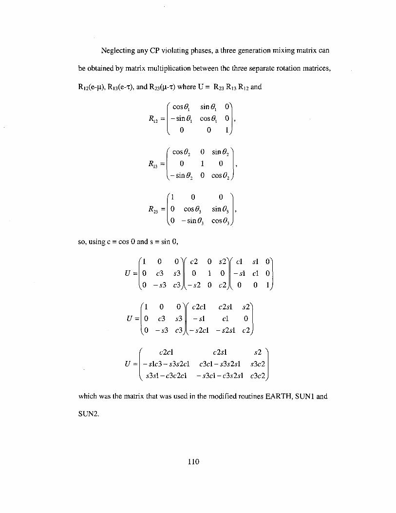
Neglecting any CP violating phases, a three generation mixing matrix can

be obtained by matrix multiplication between the three separate rotation matrices,

R12(e-/l), R13(e-T), and R23(/l-T) where U = R23 R13 R12 and

lcosO, sinO! nR!2 = -s~O! cosO!

0

lcosO,0

sinO,JR13 = 0 1 o ,

-sin 02 0 cos O2

R~ =l~0

Si:O,Jcos 03

- sin 03 cos 03

so, using c = cos 8 and s = sin 8,

U =l~0

°r2 0 S1 c1 sl OJ

c3 s3 0 1 o - sl c1 0

-s3 c3 -s2 0 c2 0 0 1

u~l~0 °Ic2c1

c2s1

S:Jc3 s3 -sl c1

-s3 c3 - s2c1 - s2s1 c2

lc2c1

U = - slc3 - s3s2c1

8381- c3c2c1

c2s1

c3c1- s3s2s1

- s3c1- c3s2s1

s2 Js3c2

c3c2

which was the matrix that was used in the modified routines EARTH, SUNI and

SUN2.

110

The electron survival probability obtained using the routine EARTH was

now found to be 0.975 which is in good agreement with values expected for the

re-conversion of mu-neutrinos into electron-neutrinos, i.e., P(v~-7Ve) = 2.5%.

After the above mixing matrix was introduced into the common block routine

SUN1, an electron neutrino survival probability of electron neutrinos propagating

through the Sun was found to be P(ve-7Ve) = 0.362 for 8 = 30°. In addition,

noticeably improved resonance curves were obtained in the output from the

program SUN2. (Compare Figures 36 and 37.)

The evolutionary probability profiles (for the SSM JCD1987) and

subsequent percent differences in P(ve-7Ve) as a function of solar radius are

shown in Figures 38 - 43. Following the lower edges of the probability

trajectories, matter enhanced resonances can be clearly seen in the region between

0.1 Ro and 0.3 Ro with a mean value around R = 0.2 Ro. When examined in

more detail, the vacuum oscillation lengths (in the region near R = Ro) are found

to be about 350 km. Using the Standard Solar Model BP2000, Figures 49 - 54

show the probability evolution and percent differences in P(ve-7Ve) with an

increased step size (discemable because of the lack of a darkened region around R

= Ro) and change in mixing angle (from 8 = 30° to 8 =33°). The lower edge of

the probability envelope dropped significantly from about 0.26 to roughly 0.17 - a

difference of approximately 0.09. (Since the survival probability is obviously

falling, the average of this value is therefore subtracted from that for the early

estimate.)

111

Nevertheless, as with the earlier percent differences in P(Ve7Ve) (Figures 40

and 43), any influence due to the electron degeneracy on the MSW effect (Figures

51 and 54) are entirely washed out by R =0.6 Ro, so there is no observable

difference in P(Ve7Ve) by the time the electron neutrinos reach the solar surface.

(The more gradual falling away of the probability difference in the region 0.5 Ro

in Figures 51 and 54 is a consequence of improved values for the FD integrals in

that region.)

A comparison was made using the output from SUN2 with some plots in

the available literature (See Figure 22 (Smimov's Figure 9).) Some of the

evolutionary trends as a function of solar density can be seen: 1) for Figures 44

and 45, there is a noticeable broadening toward the solar surface (at n =0),2) for

all of the figures (Figures 44 - 47), there is a widening of the probability envelope

with decreasing neutrino energy, and 3) there is also a steady loss of curvature as

Ev is lowered in both the SUN2 plots and Smimov's figures. (It is difficult to

compare the two lower energy graphs, however, because Smimov's density

regions have now shifted to positive values.)

Numerical calculations of the evolution of P(Ve7Ve) obtained from the

above programs have a number of features consistent with those in the literature:

(1) the matter enhanced resonance can be clearly seen in the region R =0.2 Ro,

(2) the difference between the minimum and the maximum electron neutrino

survival probabilities are within the range of other experimentally published

results (e.g., P(Ve7Ve) =0.306) [102], (3) the probability for re-conversion of v/-l's

112

passing through the Earth is the range of predicted values [130,131], (4) the

vacuum oscillation lengths found numerically (Lo - 350 kIn) are comparable with

those calculated (Lo - 300 kIn) and are correct to order of magnitude for those

measured at KamLAND (L - 200 kIn), and (5) the electron neutrino evolutionary

plots as a function of energy exhibit features that are similar to those given in

[54].

However, the numerical results from SUN2 have maxima and minima

after the resonance region that is consistently too large. This unwanted effect may

be an artifact of forcing the routine to read in SSM data stepwise, instead of

through a common block, because the routine SUNI gives good estimates of the

electron neutrino survival probability for electron neutrinos traveling through the

Sun, in addition to acceptable P(vlt ~ ve) re-conversion values for the case of

neutrinos passing through the Earth.

The modifications that were made in the numerical routine to determine

the electron survival probabilities in the case of SUN2 required introducing some

procedures that read in the data from a given SSM and allowed for two cases with

and without electron degeneracy to be calculated. The degeneracy pressure was

extracted from the SSMs with the help of the ratio of the Fermi functions

2/ 3(F3I2) giving the percent ratio of the pressure with and without electron

F1I2

degeneracy [ref. 17, p. 97]. Because the electron number density is directly

proportional to the pressure (from the ideal gas law, Pe=nekT), the same ratio of

113

Fermi functions provided a convenient way to obtain the electron neutrino

survival probabilities for the cases with and without degeneracy for a given solar

radius by directly subtracting out the electron degeneracy component from the

two different solar models (BP2000 and JCDI987).

In conclusion, I) the exponential equation describing the density profile

for the Parke and Walker analytic formula was modified to include degenerate

and non-degenerate cases. The only changes in the resulting average electron

neutrino survival probability were in the tenth decimal place, i.e., no differences

were seen in either of the final electron neutrino survival probabilities; 2) no

changes in P(ve~ve) were observed when common block density profiles with

and without electron degeneracy were introduced into the numerical routine

SUNI; and 3) calculations of the electron neutrino survival probability as a

function of distance/time found no changes with and without electron degeneracy

in P(ve~ve), once the electron neutrinos reached the solar surface. Numerical

values given by SUNI using the LMA MSW solution, i.e., P(ve~ve) =0.290, are

within 2% of that obtained using analytical methods, i.e., P(ve~ve) =0.297. Both

of these values are within 6% and 3%, respectively, with the most recently

reported experimental results from SNO: P(ve~ve) = 0.306 ± 0.026 ± 0.024.

114

8.0 Conclusion and Future Prospects

The continual progress in experimental solar neutrino physics, beginning

with the pioneering radiochemical argon experiments, have recognized the Sun as

a superb astrophysical system for advancing low energy particle physics, nuclear

physics, neutrino astronomy and, even, cosmology. Although Davis and company

were initially interested in verifying the nuclear reaction hypothesis, -- which

attempts to describe the Sun's power generation in terms of a particular sequence

of thermonuclear fusion reactions (i.e., the pp chain or the eND cycle)-- the

deficit of measured electron neutrinos observed in the Homestake argon detector

inaugurated the present period of v research marked by phenomenal growth in a

number of fields related to the physics of the stars and neutrinos.

In what turned out to be a colossal effort, investigators diligently sought to

improve upon the solar models which some believed had already reached a

developmental plateau by the 1960s. Other researchers pursued increasingly

sophisticated experiments to reduce the uncertainties of the details associated with

nuclear cross sections. In parallel with these developments, ever more refined and

reliable solar neutrino detectors experiments were built, such as the water

Cerenkov detectors, Kamiokande I and II; the radiochemical gallium detectors,

GALLEX and SAGE~ the giant SuperKamiokande light water detector~ and the

heavy water detector SNO which measures elastic scattering, neutral current and

charged current reactions - ultimately, allowing it to obtain direct evidence of

115

solar neutrino flavor conversion. There is also the neutrino accelerator

experiment, LSND (Liquid Scintillating Neutrino Detector), and the follow-up,

BooNE (Booster Neutrino Experiment) which study mu to electron oscillations

and anti-neutrino oscillations with the possibility of confirming the existence of a

fourth neutrino. Finally, the precision results from KamLAND's terrestrial

antineutrino reactor experiment in conjunction with solar neutrino data have

essentially eliminated all of the contending explanations for the solar neutrino

problem except the LMA MSW solution with a 99.73% confidence level [132].

These and other scientific advances were inspired by the solar neutrino

problem and the discovery by Mikheyev and Smimov of the phenomenon of

density dependent resonant neutrino flavor conversion. By the end of the 1980s,

many researchers realized the importance of the MSW effect as an elegant way to

resolve the solar neutrino anomaly. Because of these steady experimental and

theoretical advances, ever more detailed and demanding studies and experiments

are presently being pursued (e.g., Borexino). Some investigators have argued

that, because of the increasing precision arising from the advanced degree of

integration between astrophysics, nuclear and particle physics and solar neutrino

and solar modeling studies, a more exacting assessment of the solar (and pre-SN)

interior may be possible through neutrino astronomy -- beyond that even available

through helioseismology [57, 105].

116

The phenomenology of neutrino mixing and nonzero neutrino masses,

especially the identification of the LMA MSW solution to the solar neutrino

problem (and the results from WMAP), have had a significant impact on the

development of some grand unified theories. In retrospect, it appears that purely

leptonic interactions offer good physical systems for investigating astrophysical

applications of quantum field theories [149] because they avoid many of the

difficulties associated with quark-related interactions and they exhibit sufficient

intricacy to make them interesting, research-worthy phenomena.

8.1 Neutrinos and Cosmology

While the solar neutrino problem has been convincingly solved, the

determination of the absolute masses of the neutrinos has proved elusive. We

now know, however, that neutrinos do indeed have mass because of atmospheric

neutrino vJ1 f-7 V T oscillation measurements made at SK (hep-ex/9807003) and

direct measurements of converted solar neutrinos to other generations performed

at SNO (nucl-ex/0106015). Advanced experiments are presently being conducted

to obtain significantly improved values for the oscillation parameters, as well as

experiments to probe the absolute neutrino mass scale, such as the dedicated

tritium decay measurements (mv< 2.2 eV, Mainz) which are gradually pushing

down the upper mass limits (as the proposed KATRIN experiment with an

expected mass sensitivity of around 0.3 eV), in addition to future searches for

117

neutrinoless double beta decay (which require massive Majorana neutrinos) with

anticipated mass sensitivities of 0.01 eV [133] and mee < 0.35 eV [134].

Still, no lower bounds to neutrino masses have yet been experimentally

verified, nor has the determination been made whether or not neutrinos are

Majorana, Dirac or Weyl particles. In addition, the total number of families of

neutrinos still remains an open question. Core collapse of massive stars, such as

SN 1987A (which found my < 20 eV), may provide the best means for obtaining

mass limits from nearby (- lOkpc) future galactic supernovae [135]. Recent

precision cosmology studies have helped close in on the upper bounds of these

absolute neutrino masses (e.g., Lmy< 0.7 eV, WMAP), so that cosmology will

most likely play an important role in interpreting neutrino masses. Perhaps, even

gamma-ray bursters (GBR) may prove to be another viable astrophysical source

for studying the physics of neutrinos [136] through the detailed information that

they can provide concerning the structure and composition of pre-SN stars [137].

Conversely, the neutrino mass scale arrived at through the see-saw model

[138] (my - 0.008 eV) has provided theoretical justification for recent models of

large-scale structure of the universe. Some cosmologists, who consider a scalar

field description of the cosmological constant, A, have argued that the neutrino

mass scale for the MSW solution offers an explanation for why the vacuum

118

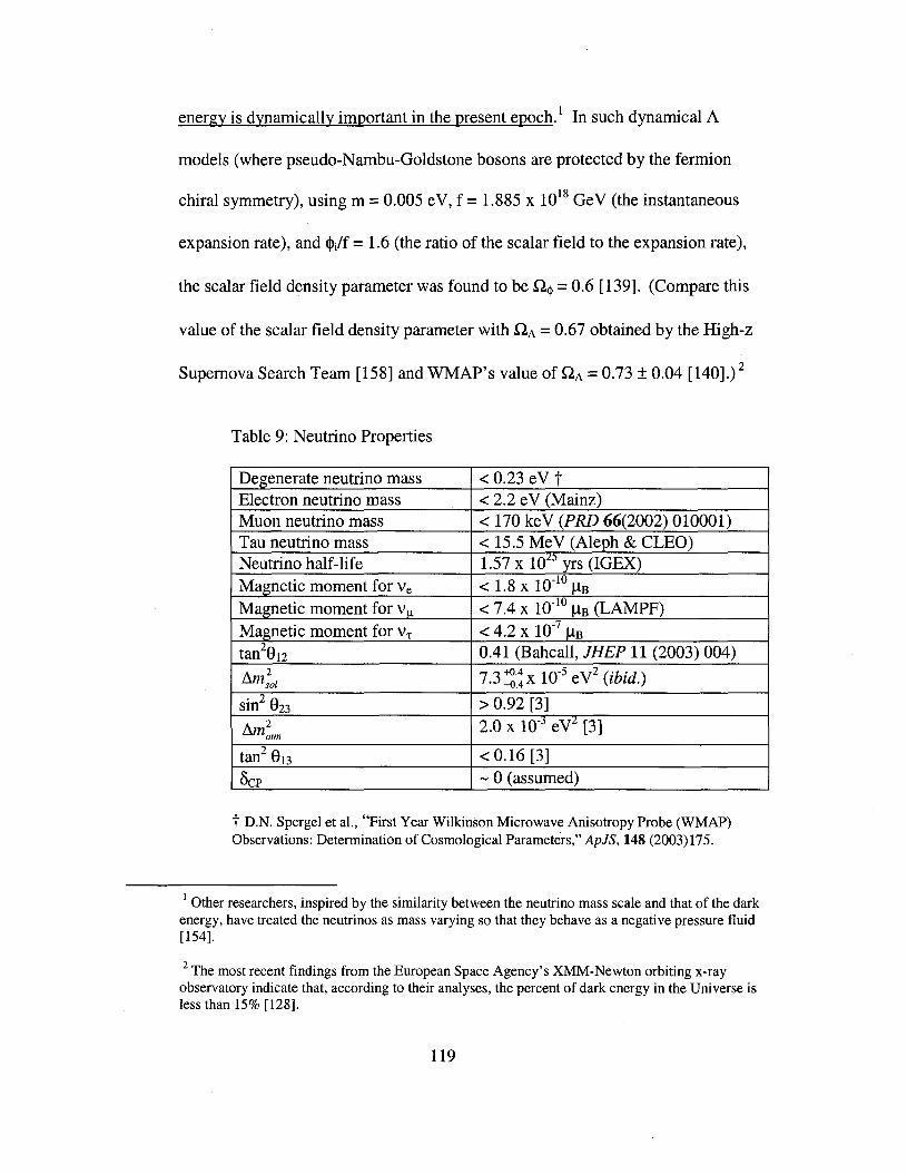
energy is dynamically important in the present epoch. 1 In such dynamical A

models (where pseudo-Nambu-Goldstone bosons are protected by the fermion

chiral symmetry), using m =0.005 eY, f =1.885 X 1018 GeY (the instantaneous

expansion rate), and <I>/f = 1.6 (the ratio of the scalar field to the expansion rate),

the scalar field density parameter was found to be Q<I> =0.6 [139]. (Compare this

value of the scalar field density parameter with Q A =0.67 obtained by the High-z

Supernova Search Team [158] and WMAP's value of QA =0.73 ± 0.04 [140].) 2

Table 9: Neutrino Properties

Degenerate neutrino mass < 0.23 eY tElectron neutrino mass < 2.2 eY (Mainz)Muon neutrino mass < 170 keY (PRD 66(2002) 010001)Tau neutrino mass < 15.5 MeY (Aleph & CLEO)Neutrino half-life 1.57 x lOL

:l yrs (IGEX)Magnetic moment for Ve < 1.8 X 10-10 IlBMagnetic moment for v Il < 7.4 X 10-10 IlB (LAMPF)Magnetic moment for V1: < 4.2 X 10-7 IlBtan2

8 12 0.41 (Bahcall, JHEP 11 (2003) 004)

/}.m~ol 7.3~~::x 10-5 ey2 (ibid.). 28 > 0.92 [3]sm 23

/}.m~tm 2.0 x lO-J eYl. [3]

tan28 13 < 0.16 [3]

OCP - 0 (assumed)

t D.N. Spergel et aI., "First Year Wilkinson Microwave Anisotropy Probe (WMAP)Observations: Determination of Cosmological Parameters," ApJS, 148 (2003) 175.

1 Other researchers, inspired by the similarity between the neutrino mass scale and that of the darkenergy, have treated the neutrinos as mass varying so that they behave as a negative pressure fluid[154].

2 The most recent findings from the European Space Agency's XMM-Newton orbiting x-rayobservatory indicate that, according to their analyses, the percent of dark energy in the Universe isless than 15% [128].

119

An alternative approach to the grand unified theoretic treatment of the see-

saw mechanism for explaining the origin of the extremely small neutrino masses

arises in left-right symmetric models (e.g., SU(2k x SU(2)R xU(l)) where the

neutrinos are found to have arbitrary but finite masses [141]. In these models

spontaneous parity nonconservation provides an explanation for understanding the

very small neutrino masses due to the fact that the suppression of V + A currents

2

are proportional to the neutrino masses. In particular, by using mv = gme andh3mWR

mWR - 300 GeV, the upper bounds on the masses of the three families of

neutrinos are found to be mv ::; 1.5 eV, mv ::; 56 keV I mv ::; 18 MeV -- valuese I" T

which compare favorably with recent experimental results: mVe

::; 2.2 eV (Mainz),

mv ::;170 keV,and mv ::;18 MeV (Aleph).I" T

Alternatively, if the lightest left-handed neutrino mass has a value below

mVe

::; O.leV, then cosmological baryon asymmetry can be achieved as long as

lepton number generation takes place in a preceding epoch where, in such non-

GUT models, the observation of a neutrino mass above mVe

- O.leV in a OvJ3J3

decay experiment would lead to the conclusion that the GUT baryon number

generating scenario must not be viable [142].

120

In minimal supersymmetric standard models supplemented with two U(l)

symmetries, it is shown that one of the symmetries breaks at 1015 GeV while the

other is broken in accordance with the MSW solution to the solar neutrino

problem through a see-saw mechanism [143]. Some researchers find that a

relatively small asymmetry between the electron neutrinos and the antielectron

neutrinos can significantly impact the ratio of the neutron to proton ratio in the

early Universe in the presence of additional degrees of freedom (i.e., including a

new energy density) [144]. By introducing three right-handed neutrinos, other

studies have found approximate values for absolute neutrino masses [145].

Altarelli and Feruglio believe that the smallness of the neutrino mass is probably

related to the fact that the neutrinos are completely neutral and are Majorana

particles [146].

In cosmological models that describe baryogenesis through leptogenesis,

the departure from equilibrium in the early Universe (the third Sakharov condition

where Band CP violation are the other two) occurs through the decay of heavy

neutrinos, i.e., through the Yukawa interaction of heavy Majorana where

yC ~ fH and yC ~ fH (with CP violation). The nonconservation of L is a

consequence of the ilL =2 term that creates the Majorana mass. The mechanism

of baryogenesis through leptogenesis is disfavored if Imvl ~ 0.1 eV, whereas the

degenerate neutrino model with Imvl ::; 0.23 eV is favored following the results

121

from KamLAND and WMAP [ref. 146, p. 9] where an experimental limit of the

Majorana mass has been given to be around 0.2 eV [147].

In nonlocal theories of baryogenesis, the bubble wall -- an expanding

region of the early Universe where the high temperature phase changes into a low

temperature phase -- interacts with the fermions with unbroken phase through a

chiral to baryon asymmetry carried by quarks and leptons. In particular, because

of the large Yukawa coupling, the main contribution to the conversion of the

chiral asymmetry to the baryon asymmetry comes from the top quark and the tau

lepton [ref. 143, p. 1486].

Even though neutrinos do not appear to have the requisite mass to account

for the closure of the Universe (-20 eV), they are of cosmological significance

because of tantalizing clues that they may hold the key to 1) the matter-antimatter

asymmetry of the Universe, 2) cosmic dark energy and 3) universal dark matter

(through their ostensible supersymmetric partner- the neutralino).

Thus, in leptoquark models, the smallness of the neutrino masses are a

consequence of processes that violate lepton number conservation so the observed

values of baryon asymmetry appear to be intrinsically bound up with neutrino

phenomenology [ref. 146, p. 10].3

3 For more details concerning the fundamental theory of neutrino masses and mixings, see [151].

122

8.2 Neutrinos and Stellar Physics

The recent advances in neutrino astronomy, especially those pertaining to

the Sun and SN 1987A, have given us an improved understanding and, in

combination with other experiments and studies, added confidence for

approaching more complex astrophysical systems. The theory of partial

degeneracy offers an effective tool for probing astrophysical objects because it is

based on well-understood physics and so introduces little error into calculations

dealing with the Sun, SNe and stars of various masses during their diverse

evolutionary phases. The physical insights that the MSW effect has provided (in

accurately describing relevant solar processes) offers increased assurance for

pursuing neutrino studies of more challenging astrophysical objects and events

such as those pertaining to pre-SN stars and the mechanism of core collapse of

massive stars. In addition, data from future neutrino experiments may possibly be

used to quantitatively investigate the existence of solar density fluctuations. In

this regard, investigations of density dependent neutrino flavor conversion may

allow for unparalleled profiling of the solar interior.

Similarities in the underlying physics describing the Sun and massive core

collapsing stars offer unique opportunities for better comprehension of pre-SN

structure and core collapse processes as well as a means of obtaining more

accurate values for the absolute mass, decay rates, and magnetic moments of

neutrinos. The Sun, for example, which only has one physically allowable critical

123

density region for a given energy neutrino, can be thought of as a simpler version

of a pre-SN star whose H-resonance region can be studied by replacing the solar

density profile with the most accurately available pre-SN density profiles, the

solar neutrino oscillation parameters with those obtained from atmospheric

studies (i.e., ~m13 and 813), in addition to making any needed modifications in the

matter enhanced weak interacting potential [43].

Since the sustained effort over the decades, beginning with

Schwarzschild's solar modeling hand calculations in the 1940s to the incredibly

sophisticated contemporary solar model calculations (in addition to neutrino and

helioseismological findings), exceptionally detailed investigations of refined

astrophysical properties and phenomena are becoming increasingly common.

Consequently, because of the ability of neutrino astronomy to help quantifiably

characterize various solar properties, one should expect an ever more detailed

understanding of the physical processes underlying stellar evolution and structure

in the near future. On the other hand, astrophysical objects, such as supernovae,

and events, such as ORBs, emerge as stellar phenomena that are ideally suited for

advancing the study of low-energy, weak interaction particle physics through

upcoming experimental neutrino astrophysical studies.

124

Table 10: Solar Parameters (from Bahcall, Rev Mod. Phys. 54 (1982) 767)

Luminosity 3.86 x 1O.j.j (3.846 x 1O.j.j t erg sec-1

Mass 1.99 x 1O.j.j (1.989 x lO.j.j)a g

Radius 6.96 x lOw (6.95508 x lOW)t cmAge ~ 4.55 x 109 (4.57 X 109)a yrCentral Density 156 g (150)a cm-1

Central Temperature 15.7 x lOb KCentral Hydrogen abundance by mass 0.355Effective surface temperature 5.78 x lOj (5.77 x lO.j)a KPrimordial mass helium abundance 0.25 ± 0.01Primordial ratio of heavy elements to H 0.0228Neutrino flux from pp reaction 6.1xlO lU (5.95xlO lU )t cm-.t sec-1

Neutrino flux from llB decay 5.6xlOb(5.05xlOb)t cm-.t sec- 1

Fraction of energy from pp chain 0.985Fraction of energy from CND cycle 0.015

:j: from Allen's Astrophysical Quantities. 4th ed., Editor, A Cox. New York: AlP Press, 2000.t from J.N. Bahcall and C. Pefia-Garay, "A road map to solar neutrino fluxes, neutrino oscillation

parameters, and tests for new physics," JHEP 11(2003)004.a NASAIMarshall Space Flight Center/Solar Physics: http://science.nasa.gov/ssl/pad/solar/

Through neutrino astrophysics, 1) the pp chain has been identified as the

primary reaction sequence powering the Sun -a low-mass star(SAGE, GALLEX);

thus, verifying the standard solar model, 2) the fundamental physical processes

underlying supernova explosions has been verified following SN 1987A (1MB,

Kamiokande I, Baksan), 3) the LMA MSW solution to the solar neutrino problem

has been confirmed (KamLAND), and 4) the deep solar (and pre-SN) interior may

been quantitatively investigated in the near future to obtain a more detailed

understanding of the core nuclear reaction rates, temperature and composition.

125

8.3 Neutrinos and Degenerate Electrons

The effects of electron degeneracy on the MSW effect in the Sun opens a

window for describing the physics of neutrino propagation in other astrophysical

systems, such as stars in the red giant stage, white dwarfs, and pre-white dwarfs

because the underlying physics describing electron degeneracy is well understood

and highly relevant for investigating such evolved stellar systems. Additionally,

there are a sufficient number of exploitable similarities between the much better

understood processes associated with the Sun -- a low mass star -- and the vastly

more complicated physics describing more massive stars, as well as those in later

stages of their evolutionary cycle, such as those undergoing core collapse -- where

the electrons, the neutrinos and the neutrons may all be in degenerate states. One

parallel in the calculations of such obviously dissimilar objects (as low mass stars

and supernovae) comes about through the fact that the critical physical parameter

in elucidating the effect of the electrons on the exiting neutrinos is the electron

density profile of the stellar system under consideration. Because the varying

(stellar and planetary) density profiles are of decisive importance in causing

neutrino flavor conversion, analyzing the effects of neutrino conversion through

static "snapshots" of the density versus stellar radii of massive stars undergoing

core collapse as a function of time may offer a tractable way of approaching the

supernova problem.4 For example, any significant increase in neutrino luminosity

4 NOTE: Complications arise in attempting to describe neutrino propagation during supernova corecollapse when all the degrees of spin are included in the calculations. See [148] for more details.

126

in regions where the MSW effect and the RSF conversion mechanism take place

may be indicative of a means whereby converted neutrinos could revive a stalled

SN shock wave.

Questions regarding the effects of partial electron degeneracy on the MSW

effect in the Sun, red giants, Si-burning pre-SN and core collapsing SN offer a

simple but discerning way to gain a more detailed understanding of the inner

workings of stars covering a spectrum of masses at various stages during their life

cycle. Similarities in the physical processes of partial degeneracy in low-mass

stars, such as the Sun, and pre-SN core collapsing stars may provide opportunities

for an increasingly refined analysis of the solar interior and improved models of

pre-SN structure.

Following the identification of the LMA MSW solution as the most

probable mechanism for explaining the deficit of solar neutrinos and the

verification of the fundamental physics underlying the Sun and supernovae,

improved calculations of the electron neutrino survival probabilities and FD

integrals may be of interest for investigating density fluctuations in SNe [105] and

the solar core [57], as well as a means for quantifying the very small relativistic

effects which arise through the Sun's partial electron degeneracy [63].

Through the use of statistical quantum field theory [149], some

investigators have considered neutrino Cerenkov emission heating of degenerate

electron plasmas as a possible mechanism to revive stalled supernova shock

127

waves [24]. Since collisional damping is reduced in the case of a degenerate

electrons gas, neutrino induced electromagnetic wave heating becomes a viable

means of solving the supernova problem because the degenerate electrons reduce

the Debye screening length -- leading to a suppression of Landau damping. For

such neutrino induced heating of the plasma to take place, the magnetic field

outside the neutrinosphere must be of the order of B ~ 1015 G and the thermal

instabilities in the region must be significant. Electron neutrinos may excite

electrostatic waves through kinetic instabilities which may be important to

reviving the stalled SN shock wave because the neutrino-electron cross section

increases with the square of the neutrino energy [155]. Astronomical

observations of magnetic fields on the order of 1016 G [4] in conjunction with

turbulent instabilities, known to follow shock wave propagation [150], give this

regeneration scenario some plausibility,S

However, recent numerical hydrodynamical calculations of spherically

symmetric core collapsing supernovae indicate that non-electron neutrino

luminosities and energies increase when cooler degenerate electron gas is

replaced by the earlier, shock-heated nondegenerate electrons [156].

5 Other approaches have identified the Zimanyi and Moszkowski equation of state [152] in themean-field approximation as favorable to the delayed explosion mechanism because of theexistence of large trapped lepton concentrations [153]

128

In conjunction with the available solar neutrino data, the small influence

of the partial degeneracy in the Sun has been investigated. Analytic and

numerical solutions showed no observable variations in the electron neutrino

survival probabilities whether degenerate electrons were included or not in the

solar density profiles of SSMs. The fact that the partially degenerate electrons

were found to have no discemable effect on the inhomogeneous density

dependent flavor conversion of neutrinos exiting the solar surface was contrary to

expectations. These negative results could be due to 1) the crudeness of the

analytic and numerical models used, 2) the fact that, in the numerical routines, the

final results are a consequence of using the adiabatic approximation (in contrast

with their actual quasi-adiabaticity), or 3) perhaps the results reflect the nature of

the phenomenon, i.e., the small percentage of degenerate electrons in the region of

the solar core has, indeed, no influence on the MSW effect in the Sun.6

6 Table 2 in [72] implies that the non-ideal gas effects due to electron degeneracy in the OPALequation of state also have no noticeable influence, according to their studies.

129

APPENDIX A

Fierz transformation of the interaction Hamiltonian

Let 'If represent a four-component Dirac spinor, and r represent the set of

any physically allowable combination of the Dirac matrices {I, yll, yl!o.{, 'I, and

a llV} which stand for the scalar, polar vector, axial (or, pseudo) vector,

pseudoscalar and tensorial gamma matices, respectively. In four-component

notation, a four-particle interaction can be written as

or, more generally

where r K and r L correspond to any of the 16 combination of Dirac matrices.

After compacting the orthonormal trace formulae Tr{l} =4, Tr{yS ys}=4,

matrix M into a complete orthonormal set, i.e., M =L ~K r K ' the trace of theK

product of the matrix and the generalized gamma matrices is given by

Tr(MrJ =L~KTr(rKrJ.K

But, since Tr{rKrJ= 4JKL , then after collapsing the summation

130

In component form, the above coefficients can be written as

Rewriting the four particle interaction in terms of the components of the

respective column vectors and matrices,

and expressing the bilinear If/fJ (2)lf/o (3) as the matrix M fJo ' and repeating the

same normalization procedure using the trace formulae in the general case, we

find If/fJlf/0 =Lr;K (rK) ,so that

K fJO

j: 1 ( (K)) 1 K 1 K .~ K =- Tr M fJo r ofJ =- M fJo (r )0fJ =-If/fJlf/0 (r )ofJ Rearrangmg terms such

4 4 4 '

spinors anticommute, {If/fJ' If/o} = 0 , i.e., If/fJlf/0 = -If/olf/fJ ' allows the four particle

interaction term to be written as

Similarly, to move If/(4) to the left of If/ (3) introduces another minus sign, giving

Dropping the indices leaves

131

Thus the general Fierz transformation can be written as

(¥/(l)r K ¥/(2)X¥/(3)rdl/(4») = L;~~ (¥/(l)rM ¥/(4)X¥/(3)rN ¥/(2»)M,N

j:KL 1 (M K N L) 1 (J:' J:')where [30] ~MN =-Tr r r r r =- 4UMK 4uNL =1, so16 16

More specifically, for the case of electron-neutrino scattering

132

ApPENDIX B

Derivation of the Energy Rate Formula1

The reaction rate formula can be written as Rrx =If cr(v)vdnr(v)dnx(v)

where dnrCv) and dnx(v) represent the number of nuclei and particles per cubic

centimeter represented as volume elements in velocity space, cr(v) is the cross-

section for the reaction which describes the probability of the interaction as a

function of the particles' velocities. A Maxwell-Boltzmann (MB) distribution is

assumed valid because of the relatively low densities in the solar interior. (Yet,

see quotation on page 50 above.) Writing the particle number volume elements

in velocity space as an MB distribution, we find:

for the particle r and a similar expression for the target nuclei X. The reaction

rate formula becomes upon substitution

( )3/2 ( )3/2 ~ ~ [( 2 2 )}R =n ~ n -.!!!L ffexp - mrVr +mxvx (v)vd 3v d 3v

rX r 27lkT x 27lkT 2kT r xo 0

Using center-of-mass velocity V = (mrvr+mx vx)/(mr+mx) and the

relative velocity v =Vr - vx, we can substitute Vr =V + mxv /(mr + mx) and

1 See Huang and Yu, Stellar Astrophysics (1998)

133

Vx =Y - mxv /(mr + mx) into the equation for the conservation of kinetic energy

to obtain mrv2+ mxv2= (mr + mx)y2+ mv2where m is the reduced mass given

by m =mrmx/(mr+mx). In addition to these substitutions, the replacement of the

volume elements of the velocity derivatives using these new coordinates, can be

written as d3vr d3vx =4ny2dY (4nv2dv). The resulting reaction formula becomes

where K(r,X) = nr(mrl2nkT)3I2nx(mx/2nkT)3/2 .

The second of the two integrals can be written in terms of energy through the

equations E =Ih mv2 and dE =mvdv so v =.J2E / m and dv =dE / .J2mE .

Upon substitution, the second integral becomes

Setting a =~ in the first integral, one obtains fe-av2V2dV. Making a change2kT 0

of variable where f =aV 2, so V = ~ and dV = db, then the first integralV-;; 2vaf

1 =f -~ r.i j: _ reV 2)becomes-m e vsd~ - 3/2' or

2a 0 2a

.J1i (2kT)3/2

2 M 3/ 2

Multiplying the two solutions (ex) and (~) gives

134

(ex).

~( )

3/2=1r 2kT fe-ElkT E1/ 2avdE.2 mM 0

Returning now to the equation for the reaction rate, we find

becomes

R =n n =f ~ 1 e-ElkT El/2avdErX r X 0 V-;- (kT)3/2

Letting I(E) ~ ~2 1,,, e-mTE'''dE, the reaction rate cao be written1r (kT)

=

RrX =nrnx(av) where the reaction probability is (av)= ff(E)avdE whoseo

physical meaning is described as the average probability for a pair of particles in a

cubic centimeter to participate in a nuclear reaction.

The energy generation rate, c, defined as the energy generated by one

gram of stellar matter in one second can be written in ergs/gls as

For two identical nuclei interacting, then r =X and nr nx =nr(nr - 1)/2::::: nr2/2, so

n.n· ( )the reaction rate formula can be rewritten as Rij =-'_J_ av where Oij is a. 1+ c:5jj

Kronecker delta. Since, ni = pNAXi the energy generation equation becomes

135

The product crv is equal to the product of the probability of tunneling

through the Coulomb barrier and the probability of the nuclei engaging in a

nuclear reaction, crv = Pp PN • For a non-resonant reaction the cross section

probability, SeE), is just a constant, so PN =So while the probability for quantum

mechanical tunneling is given by Pp = f-fE-1I2e-b/./E where b represents the

where the reaction probability decreases with increasing charge and for

decreasing energy or temperature.

Substituting the product into the reaction probability formula gives

~ 2f-f 1 ~(av) = ff(E)OVdE =So r= - 3/2 fexp[-EI kT -blJE]dE.o ~n m~T) 0

Obviously, when the term in the exponent is equal to zero, the reaction probability

will be a maximum. In other words, when E/kT + b/-VE is a minimum then the

integrand will be a maximum, i.e., ..!!-(.£+ ~J =O. When this condition isdE kT ~E

( )

2/3

satisfied, the result is l/kT - (b12)E-3/2 =0 so E3

/2 =(bkT12), or Emax = b~T

This form of the equation provides an order of magnitude approximation of the

energy associated with the Gamow peak which describes the optimum value for

136

the energy of the particles that participate in the nuclear energy generating

processes in the Sun. For the p + p reaction, b; ~m; (41<'e' I he0) ;

(27 J1I2 ( 38 2J1.67xlO- kg (39.5)(2.56xlO- C =4.87xlO-6~m/ s and so

2 (8.85xlO-12 C 2/ Nm 2 vAg

( J2/3

_ (bkT)2/3 _ (4.87xlO-6.[kim/ s)(1.38xlO-23 J / K)(1.57x107K)Emax - - ,so

2 2

Emax =(5.28xlO-22)o.6667 =6.52 X 10-15 J:::: 40 keY. This value has the same order

of magnitude as that given by Schwarzschild earlier of 20 keV. A better

approximation can be obtained by transforming the exponential term at the top of

the page into the form of a Gaussian. The width of the Gamow peak can also be

4£5/4derived, where it is found to be Llli = ;;x [ref. 66, p. 161].

v3b

Finally, to put the nuclear energy generation equation into a slightly more

explicit form, the values for NA =6.022 X 1023 and Q (MeV) into units of ergs, Q

=(106 eV)(1.602xlO-19 J/eV)(107 ergs/J) =1.6 x 10-7 ergs give

The final form for the nuclear reaction rate for the p + P step can be written as

has the distinctive T 2/3 and Tl/3 temperature dependences mentioned earlier and

requires extra terms to approximate the non-gaussian shape of the Gamow peak.

137

ApPENDIXC

Solution of the neutrino eigenvalue problem

Written in the form of an eigenvalue equation, the Schrodinger equation

has nontrivial solutions when

det(H f (t) - Li(f)) =0

where the matter modified Hamiltonian in the flavor basis is

1 [- ~ cos 28 + A ~ sin 28JH - 2 2

f -- ~ ~ .2£ -sin 28 -cos28

2 2

Thus, the determinantal equation takes the form

~ 1--cos28+-A-A

4£ 2£

~sin284£

~sin284£ =0~

-cos28-A4£

so (-~COS28+~A-A)(~COS28-A)-(~sin28)2 =04£ 4£ 4£ 4£

and the corresponding quadratic secular equation is

with solutions is

A=~±_1_~A2-2A~cos28+(~cos28Y+(~sin28Y4£ 4£

138

APPENDIXD

Transform of the neutrino vacuum propagation equation

In the basis of mass eigenstates, the evolution equation for the case of

vacuum oscillations can be written in the form of the Schrodinger-like equation

.d Hl-lf/ = If/dt m m

(

VI (t)Jwhere If/m represents the Dirac spinor If/m = .

v2 (t)To obtain the equation

expressing the neutrino evolution in the flavor basis, a unitary transformation is

made using

H'=UHU+

where the neutrino mixing matrix is given by

U =(cos 8 - sin 8Jsin8 cos8

and 8 is the vacuum mixing angle. The Hamiltonian, H, defined through the

equation

becomes

+ (cos 8 - sin 8J M 2 ( cos 8 sin 8JH'=UHU = -sin8 cos8 2p -sin8 cos8

139

=_1(COS a - sin oJ(mt2

2p sin a cos a 0

1 (m12 cos 2 a+ m~ sin 2 a

= 2p (m12

- m~ )sin acos a

The first diagonal term can be expanded as

o )( cos a sin OJm~ -sinO cosO

(m{ - m~ )sin ocos 0)2 2 2 2 •

m1 sin 0+ m2 cos a

m12 cos 2 a+ m~ sin 2 a=.!. (m1

2 cos 2 a+ m12 cos 2 a+ m~ sin 2 a+ m~ sin 2 0)

2

and rewritten as

=~ {m.' eo,'l1+ m,' ,in 2 (} +m; co,' (} +m; ,in 2 (} +m; ,in' (})+ ( m; ; m,' )'in' (} - co,' (})

and similarly for the second diagonal term, m{ sin 2 0+ m~ cos 2 O. Using the

notation ~ =m~ - m~ for the square of the neutrino mass difference, the first

diagonal term now takes the form

(m12

+ m~ Xcos 2 a+ sin 2 0) ~ (. 2 a 2 a) (m~ + mn ~ (. 2 a 2 a)-'--"---..;;...:..."'--------!.. + - sm - cos = + - sm - cos

2 2 2 2

so the transformed Hamiltonian is given by

[

(m2

+m2

) ~(. ) (). ]1 1 2 +- sm 2 0-cos 2 a m12-m~ smocoso

H'=- 2 22 . m2 +m 2

~ .'P (m,' - m;)'10 (}eo,(} ( '2 ,) +2(co,,(} - '10' (})

or H'= m{ +m~ (1 0J+~(-COS20 sin20J.4pOI 4p sin 20 cos 20

140

ApPENDIXE

Transform of the neutrino matter propagation equation

Beginning with the Schrodinger-like equation (since \If represents a Dirac

spinor, IfIj = (~:), and not a wavefunction)

where Ifff represents the state vector in the flavor basis and

1[- ~cos2B+ A ~ Sin2BJH - 2 2

f -- ~ ~ ,2£ -sinZB -cosZB

2 2

Acting on the interaction evolution equation with the mixing matrix in matter

from the left, and using H f =UM HU~ to transform the matrix into the diagonal

basis leads to

Since U~UM =1 and .!!:- (UMiff) =UM dIff + Iff dUM, the above can be written asdt dt dt

'u dlff -(U H ,dUM)1 -- -1-- Iff 'Mdt M dt

Now, acting with U~ from the left and using the unitarity property gives

141

.dlf/ -(H ·U+ dUM)1-- -1 -- If/.dt M dt

The second term on the right hand side can be written explicitly as

+ dUM (coseMU --=M dt -sin eM

where the time derivative acting on UM via the chain rule, i.e.,

d .-cos eM (t) =-sin eM (t)eM ' sodt

and

+ dUM _ . (coseMuM---eMdt -sin eM

-coseMJ.-sin eM

Multiplication of the two matrices gives

(- cos eM sin eM +sin eM cos eM

sin 2 eM +cos 2 eM- cos

2eM - sin 2 eM J (0 -olJ

sin eM cos eM - cos eM sin eM - 1

so

Thus, in the diagonal basis, the spinor propagation equation (using x =t) becomes

[[

- 2 () • deM J]d 1 m1 x 1--

. dx1-lf/ =- If/dx m 2E -i d:; m~(x) m

where ~ 2 =m;2 •. .

142

FIGURES

Figure 1. Partial, Complete and Maxwell-Boltmann Distributions

f(p)

f(p)

8 _10'5

143

II

I/

//

.Ii/ I

II

Figure 2. Fermi distribution function versus energy

~kT~I I, I

~IT=O

T>O

144

Figure 3. Masses of two flavors of neutrinos as a function of density

p

FIG. L The masses of two navors of neutrinos as a func­tion of d.ensity. The curves ne~rly cross atone point. Theelectron-antineutrino mass Vf' is also shown.

(from H.A. Bethe, Phys. Rev. Lett. 56 (1986) 1305)

145

Figure 4. Feynman diagrams for neutrino-electron scattering processes.

+

(a)

( b)

146

Figure 5. MS triangle

,00 I 1-.-._",~.__,L_,.~_~_~_..L.~..J..,J,,~ -JI-.-.-L--L-L....l.....JLLU

,OJ

-EI

WI\!aOt

I

sin260

FIG. 1. Probabinty-oontour plot for detecting an electronneutrino at the Earth which was produced in the solar inte­rior.

(from Parke Phys. Rev. Lett. 57 (1986) 1275)

147

Figure 6. Partial electron degeneracy in the solar core

-2

-1

- 4 t----'----.a...-----L.~__1

~ -3

1016 1015 1014P[Pal

148

Figure 7. Electron number density difference with and without degeneracy

6

(Y)(

Eu

........LD 4(\J

(

0.--i

X

Q)

z2

0.0 0.1

149

Figure 8. Solar density profile (BP2000)

150

(Y)100

<Eu

.........0'

0::r::~

50

0l--.l---L---l.---L-l_1.-.l--...L.-....J-.-L--l_L--.L--L---l.---L..---I_.l-....J.--....J0.0 0.1 0.2 0.3 0.4

R/Ro

150

Figure 9. Partial electron degeneracy in the solar core.

1.5

+>c(I)

() 1.0L(I)

(L

0.5

0.1 0.2R/Ro

151

0.3 0.4

Figure 10. Solar density profile (JCD1987)

150

100(Y)<Eu"-'--'0

..c.fr:

50

0.1 0.2R/Ro

0.3 0.4

152

Figure 11. Comparison of density profiles for two SSMs

140

(Y)(

E.

~ 120o

..c0::::

100

0.02

153

0.04R/Ro

0.06 0.08 0.10

Figure 12. The log of electron density versus solar radius (BP2000)(astro-ph/OO10346)

4

3log(njN.) vs. RIRE)

2 BP2000

~ 0Ill>~

-1

-2

-3

-4 a

Fig. 8.... The e!pctron numher density, fie, versus solar radius for the Standard so]ar model(BP2000). The stl'llight·Jine fit shown in Figurp S is an approximation, Eq. (14), given hy BahmH(1989). EqUlltioll (14) hilS boon used previously in many Ilna]yses of lllllttereffocts Oil solllr neutrino

, propagl1tion. Precise nUlllerir~,j vahle, for lle Ilre available Ilt

154

Figure 13. Gamow peak (theoretical)

155

E

Figure 14. Gamow peak (experimental)

- »!•.a 1.~S 16...J 1~..j uI

10t.-~ I

&

..~

010

o .......A(&II)• K.._ d .... 11.!I87)• o-n.b...d.L (1971)

- ~A(l9!I8)BIR: N..aII- """""(1998)5......1 NoocWl1it

Fig. 1 Astrophysical factor S(E) for the 3HeeHe,2p)'1Ie reaction

(from R. Bonetti et al., "First Measurement of the 3HeeHe,2p)4He CrossSection down to the Lower Edge of the Solar Gamow Peak,"nucl-exl9902004)

156

Figure 15. Log of electron density versus solar radius (sterile neutrinos) (BP2000)(astra-ph/DO10346)

-4 0 0.1 0.2 0.3 0.4 0.5 0.6 0.' 0.8 0.9R/Re

3

2

-2

-3

log(n.wrne!NA) vs. R/Re

BP2000

Fig. 9.HH The number density, fislerile, of scatterers of sterile neutrinos v'Jrsm solar nuHIl8 for tbeStandard solar model (BP2000). The straight line in Figure [I is given by an equation of the sameform as Eft. (14) excrpt that the coeffident for n~terite/N.4 is 22:J (instead of 245 for nelN'l)'

157

Figure 16. Solar neutrino flux

(From A.B. Balantekin, "Neutrinos in Stochastic Media: From Sun to Core­Collapse Supernovae," hep-ph/Ol09163: Solar Neutrino Flux)

10' ------------,

10Ii, (MeV)

FIG It[ 1. Sobr .uun. Ilul. Th< <ffi6~ .. th< rnJ"'lioa flt' ,''' SllIxIInI Sob. M~I ",.u.: kil by I!l< b1xk hondTht IIld clllrd..uon '.'1111110 ftlnWt II'I',~.. ~bylh<>Ia.'W_ nh<_~i. dw lIlOl1l1orllb<oIWaI ..... Ih<I'f<di<"'"'u "'~SlI\""pI\llxlIl<l~ ,.....~ 111<6_""" tU.t=s, ,,-$(\-1..JlInl8:OJ 11l<'JW""'Sl'-i"'J"Iioddv.lo..1Ia01WIM01 cb;<mdia~~~ l..lmlm<hlIWfmr~ihr "I'<fl..,..j<m1f ",ullaril>1lllllw...~II.:cbihlIllmc~ I "~dilcllh<l<ltIl_ .....~.I<Il.......... ,""h"Oi:II~~ ...~.~I"'s.duQN<w!,.,llhotMloly....L ~lIIIdr

we.!I!R<\<If<body,.I>.'li1)-.a1 tin...1''''1".1 6J:l1f" ....1 """"

158

Figure 17. Neutrino production as a function of radius

IGHeulriDo Production

....... Radhu.

PIG. t. Neut.riao procIucdott at • ftIDotlon of rHi-. The .......tioa of neu.trinOI that oriJiute in eIdt fracdoa or the IOIar ra­di. :ia (dF1ux/d(R/It(j»))[d(R/Ra)). The ....... Wamrateathe prodbCdon fl'IIction tor '». 'Be, H, and bep DeUtrlJwJs forthe «aDdu'd IOIIt model delcribed ia Sec. V.B and Table XI.

Rev. Mod. Phy&. VOl. la, Ho. 2. AtWI 1_

159

Figure 18. Calculated neutrino spectra

0.1 0.2 0.4 0.6 2 10 20

10 12 1r-,==--rF;";"';;;";::';:;:;;';m-:I~

1811

1010

109

108

~ J01U-

10'

105

a 4

105

~.~.:.;.~.

102

101 O·~.1':""'::::..:.J.:~:c...:JILLJ~r:::.u+:li....:J.:...LL:~~~~..:u;~

NeutrIno energy (MeV)

Figure 17: Calculated Neutrino Spectrafrom <http://borex.lngs.infn.it/aboutlborexinof.html>

160

Figure 19. Temperature dependence on solar neutrino fluxes

(6)

I" 11$.7 1$.1 15.1 .8

log 4>(hep) vs. Tc • ....

j-!j

~

j

13j

"'. Ii,

lS.s 11.1

Tc

..6'

!! '" I 1!

..,.;i.;lJJiir,:....{.,

~:~~~ .. ' .-.. . .

log 4>(7B.) vs. Tc

u-

U~i;C2:--""""":-:3'--'::-"-:-'-'":":-:'~""'::"~'-~I:;;'-;7~";';::";;-""-;;";;'~-;"(6) Tc

,.G.N-

e.ate

r .,[~

C.llc..~ .~

~..['M[

f I , " .0.0..U .U IU(4)

lUL'

"

..

Tc

~

'1..J1

~

.I, ,,' " ,,,,,,,,,,,,,,,,,,,]1$.4 JU 15.1 67 t5.8 J~. "

log 4>("B) vs. Tc

(a)

tui...

"•o.•~

t.l

o.r;....

t~

"UI-

t0.5 t. ,,,! , , I , !

15.1 15.2 11.3

T' ., ., ..~~;w~:'j~ ..~ .,.~ 1

~ ~ • a 1~3 ..J

:1',,,,,,""""""",',,""""'" J1$.2 1$.3 1$.4 11.5 15.1 1$.'1' 1i8 Is.a

F!pre '.2 Temperalure depeade""e or lhe '8 ... pp aelIIrlao BuxesIn figure 6.2•• the logarithm of the calculated"B _rino Bux is shownas a function of central lPmperature for the 1& solar models that werecalculated by Bahcall and l'lrich (1988). for this&c-.the temperature isgiven in units of 10" K and the ftux in units of 10'em-· .-'. In Figure 6.2b.the logarithm of the pp neutrino ftux is disp~ .. a function of centraltemperature for the same 1000 solar models. for Ibis figure. the 8ux isexpressed in units of 1010 cm-2 5-1: the unit oI'&emperature is the sameas for figure 6.20

r_ U Tempenlure depeBdell<e of lhe bep _ T.Be _.rino 8""esIn figure 6.3a. the Iogarithm of the calculated hop neumno 8ux IS shown as• function of central temperattUe for the 1000 solar models that. were cal-­culated b,' Bahcall and l'\rich (1988). In figure 6.36. lhe logarithm of theTae Df'utrlno 8ux is displayed as a (unction of central temperature for thesame 1000 solar models. The unit of temperature is 10' K. for figure 6.3a.the fluxes are expressed in units of loJ cm-t S-I and for Figure 6.36. inunits of lOS' cm-2 5- 1•

161

Figure 20. Level crossing diagram for SN neutrinos

normal hierarchy

v'f

ne

L-resonance

mI-V_3 -+~.....---V~(I;l

E~U V2

~

vacuum SN core

Figure 2. Level crossing diagram for normal mass hierarchies(from Takahashi and Sato, Prog. Theor. Phys. 109 (2003) 921)

162

Figure 21. Pre-SN density profile for 15 Mo star

H

10.1radius(sofar radius)

O+C HeO+Ne+Mg1x106r---........--.........-----+-----.

lOOO(l(l

10000

1000iQ 100

i 1~v

0.1

0.010.001""- .....

0.01

FIG. 3. Density profile of the presupemova star model used inthe paper [20]. The progenitor mass is set to be 15M0 .

(from Takahashi et aI., Phys. Rev. D 64 (2001) 093004 where ref. 20 isS.B. Woosley and T.A. Weaver, Ap. J. SuppI. 101 (1995) 181)

163

Figure 22. Evolution of neutrinos with different energies

--------_._._---------

-----..---.~.......-.....""'--.....

.---_.....-_ .._-_ .._----------_.

"

Figure 9: The !!I'olutioll of tllP l!eutrinn-; with dill'enmt, PIlergies in the Sun, Shown arethe dep()IHlenGes of the ilveillged value of the surviv1u prob'lbility (dashed lines), as well asInaxinml Hnd mininml values of the probability (solid lines) OIl n. Neutrino is produced illtho center of th,) SUll. The density df1creases from the loft to the right. The rOSOIlaJlce eisat n = O. The probability is the oBl:illatory curve which is iliS< Tibed in the band betweenpmux and pmi". Upper left pallel: E 14;\leV, upper right panel: E fi l\JeV, lower leftpimP] E = 2 !vleV, lower right panel E= O.8(j MeV.

(from Smimov hep-ph/0305106)

164

Figure 23. Survival probabilities

Figure f): The dependl~nCt~ of the average probability (dashed line) and the depth ofoscillations (IJ""'X, pm;n solid lines) OIl n for no = --5. The reSOIlHnee layer corresponds to11. O. For tan2 (/ "'. 0.4 (large mixjn~; MSW solution) the evolution stops at 11, '" 0.47.

165

Figure 24. Profile of survival probabilities

..••

• 2

., 1., ,.S

Figure 8: Profile of the effect. Dependence or the surviwd proof\bility on nentrino energyfor the best fit values of parameters and production in the center of the Sun (solid line).For tJ.m2 =. 7.10 5 e\'2. x ~= 2 corresponds w E ~ 10 MeV. The dashed line shows theilveraging effeet over the production region R O.1R."". The Earth matter regenerationeffect is not included.

Figure 25. Level-crossing

Figure 3: Level crossing scheme..Dependence of the eigenvalues of the Hamiltonian inIllatter, HIm lutd H2rn , on the ratio x == lv/lo for t\VO different values of VRenUIn Inixingsin2 20 =···0.825 (solid, blue lines) and sin2 0=· O.OS (dashed, red lines).

166

Figure 26. MSW Contour Plot

1r &.1 G2 U U 0.& 0.1 U 0.1 0.1 1tit

,''' 0.1 OJ! U OA U U 0.7 U ... 1til

Figure 7: The be,'t fit points and t.he allowed regions (at. different C.L.) of the 06Cillationparameters (at different C.L.) from the global fit of tile solar neutrino data (left), and froIllthe combined analysis of the solar neutrino data and KamLAND (rignt).

(Smimov hep-phl03050106)

167

Figure 27. Electron number densityvs. solar radius (JCD1987)

6.0.1025

5.0.1025

4.0.1025

(Y)<Eu

:::::3.0.1025Q)

z

2.0.1025

1.0.1025

0.0 0.1

168

0.2R/Ro

0.3 0.4

Figure 28. Electron number density vs. solar radius (BP2000)

6.0,1025

5.0.1025

4.0,10 25(Y)

(

Eu

~3.0·1025L:­0:::

2.0,1025

1.0.1025

0.0 0.1

169

0.2R/Ro

0.3 0.4

Figure 29. Electron number densities for BP2000 (upper) & JCD1987 (lower)

5.0.1025

4.0.1025

(Y)

~3.0.1025"-~

o.ccr

2.0.1025

1.0.1025

0.050 0.075 0.100

170

0.125R/Ro

0.150 0.175 0.200

Figure 30. Induced mass A vs. sin2 20 M showing matter induced resonance effects

AFIG. 2. Plot of sin220"p where Om's the etfectiveneutrino mix­ing angle in matter. as a function of A. the induced electron­neutrino mass. Here we take mj -m f==3.0 and sin28=0.03.

(from Kuo and Pantaleone Rev. Mod. Phys. 61 (1989) 947)

171

Figure 31. A vs. sin2 28M using LMA parameters where Pc=35 glee & Rc= 0.2 Ro

0.8

EI

10 0.6+.>(l)

..c+.>•(\J

(\J0.4(

c..-i(I)

0.2

0.5

172

1.0A

1.5 2.0

Figure 32. Neutrino level crossing diagram using LMA parameters

2.01.51.0A

0.5

1.25

a.aa L--...L.----'-----'---'-_'--...L.----'-------'---'-_'---'-----'------'----'_-'-----'-------'-----L_L--J

0.0

0.25

1.00

(\J<J.)<n 0.75<n10E

0.50

173

Figure 33. The solar pp chain

2 + 2 .p+p .... H+e +p p+p+e· .... H+p

t_-f-_t99.75% 0.25%

2H + P_JHe +,.86% t 14%t~---_"--:"':'t

\Ie + JHe ...."He +2p JHe + "He ....7& +.,

t 0.11%

t7Be + p ....HB +-r

t3n .....Rae· +e+ +.,

ppl ppll ppIlI

I From Balantekin and Haxton, "Solar, Supernova and Atmospheric Neutrinos,"nucl-th/9903038.

174

Figure 34. Degenerate density vs. exponential density profiles

150

100(Y)

:>- (

.j...> E..... uII)

c '-(J) ~

0 0...c.0::::

50

ol-.L-----L--L----l-~:L----L--l.----L-~"f___~::::L:::±:~=:l::::==!=o 1.0.108 2.0.108 3.0.108 4.0.10 8

R A = 245 alpha = 10.54

175

Figure 35. Degenerate vs. nondegenerate exponential profiles

150

100

50

oL-..L.---l..-..J--rf--L-....I---L--.L~:::::~~=~:=..Jo 1.0.108 2.0.108 3.0.108 4.0.108

R

176

Figure 36. Evolution of P(ve~ ve) using incorrect mixing matrix

0.8

0.6:>1\II

:>

0....

0.4

0.2

0.2 0.4R/Ro

177

0.6E= 10 MeV

0.8 1.0

Figure 37. Evolution of P(ve~ ve) using corrected mixing matrix

1.0

0.8

~ 0.6II::>

Q...

0.4

0.2

0.2 0.4R/Ro

178

0.6 0.8E= 10 MeV

1.0

Figure 38. Evolution of P(ve ---7 ve) using JeD SSM (Degenerate case) Step = 1

1.0

:>1\II

:>

a...

0.8

0.6

0.4

0.2

0.2R/Ro

0.4 0.6 0.8 1.0E = 10 MeV --> sdens=rho(1+Xl/2

179

Figure 39. Evolution of P(ve~ ve) using JeD SSM (Nondegen case) Step =1

1.0

0.8

> 0.61\

II

>0.-

0.4

0.2

0.2R/Ro

0.4 0.6 0.8 1.0E = 10 MeV n) sdens=rho(l+XJ/2

180

Figure 40. Percent difference in P(ve -7 ve) using JeD SSM (Step = 1)

100

> 50/\,,>

CLICJ+->......Q)

0~

0

-50

0.0 0.2R/Ro

0.4E= 10 MeV

181

0.6 0.8-->sdens=rholl + Xl/2

1.0

Figure 41. Evolution of P(ve~ ve) using JeD SSM (Degenerate case) Step =lh

1.0

0.8

::>- 0.6/\II

::>-

0.-- 0.4

0.2 0.4 0.6 0.8 1.0E = 10 MeV --) sdens=rhofl >XJ/2 >LIN.INTERp·

0.2

o.0 '-----J----I.-..L-L.....L.......L-.L.....J----I.-..L-L.....L.......L-.l.-JL....L-..L---l-.....L.......L-.L.....JL....L-..L--L---l.--LJ

0.0R/Ro

182

Figure 42. Evolution of P(ve -7 ve) using JeD SSM (Nondegen case) Step =Y2

1.0

0.8

> 0.6/\II

>0....

0.4

0.2

o.0 L-L---'---L......L-L.-.L---'---L......L-L....L-L--L-..L-Jl-L-L--L-..L-L..L~..-I---l.-L...1-LJ

0.0 0.2 0.4 0.6 0.8 1.0R/Ro E = 10 MeV --> sdens=rhoO' Xl/2 ·UN.INTERP-

183

Figure 43. Percent difference in P(ve --7 ve) using JeD SSM (Step =1)

100

:>- 501\II

:>-(L

10+-'

Q)

0~

0

-50

0.0R/Ro

0.2 0.4 0.6 0.8 1.0E= 10 MeV u)sdens=rhoC1+X)/2 LIN.INTERP-

184

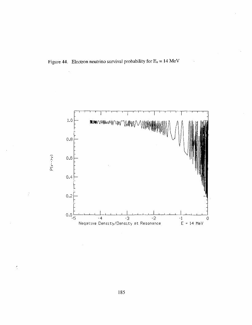
Figure 44. Electron neutrino survival probability for Ev = 14 MeV

1.0

-1 0E = 14 MeV

>1\I.>

Q...

0.8

0.6

0.4

0.2

o.0 ~--.L---l....-L---l-....L-.l..--l.--.I--1.--L-.L-..l.--L-..l.-.L.-JL...-L--L........l-L-L........L-~

-5 -4 -3 -2NegatIve DensIty/DensIty at Resonance

185

Figure 45. Electron neutrino survival probability for Ev = 6 MeV

1.0

>1\

I,>

0...

0.8

0.6

0.4

0.2

-1 0E = 6 MeV

o.0 ~'--'---'----L.----'---'---'--....l...--'--.l..--L--J-.l---L--L---L-L.--'--....L-...L-...l.....-.l..--L--Jl...-.i

-5 -4 -3 -2NegatIve DensIty/DensIty at Resonance

186

Figure 46. Electron neutrino survival probability for Ev =2 MeV

1.0

:>/\II

:>

0...

0.8

0.6

0.4

0.2

-1 0E = 2 MeV

o.0 ::--,-.-L-..L--.L---L-...L-L-.J.-L-L--.L---L-...L-.L-1--L---L.--.L-....L.......l--L-.J.-L---L..J

-5 -4 -3 -2NegatIve DensIty/DensIty at Resonance

187

Figure 47. Electron neutrino survival probability for Ev=O.86 MeV

1.0

>/\II

>(L

0.8

0.6

0.4

0.2

-1 0E = 0.86 MeV

o.0 L-.J'---.l.-----L.........L-L-L-l.---L.-...L-L-l.---l-----l.---L-L-L-L.--l.---L.-...l.-...L-.L-L-...JL...J

-5 -4 -3 -2NegatIve DensIty/DensIty at Resonance

188

Figure 48. Interpolated ratio of FD integrals

1.5

oLL

1.0

0.5

0.0 0.1R/Ro

189

0.3E= 10 MeV

0.4-->F'erm12.F'

0.5

Figure 49. Evolution of P(ve --7 ve) using BP SSM (Degenerate case) Step =1

1.0

0.8

> 0.6I,>

0...

0.4

0.2

0.2 0.4R/Ro

190

0.6 0.8E ; 10 MeV

1.0

Figure 50. Evolution of P(ve ~ ve) using BP SSM (Nondegen case) Step = 1

1.0

0.8

7' 0.6,>

(L

0.4

0.2

0.2 0.4R/Ro

191

0.6 0.8E = 10 MeV

1.0

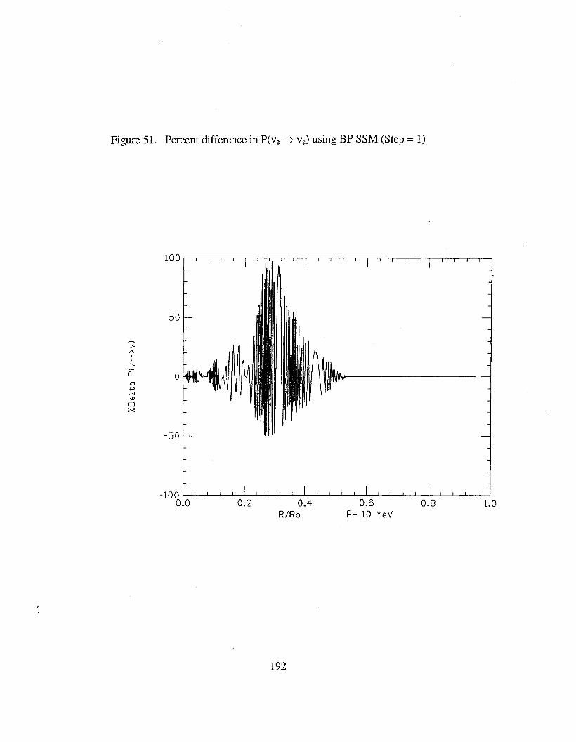
Figure 51. Percent difference in P(ve~ ve) using BP SSM (Step =1)

50

:>1\,I

:>

0... 0iO+>.......Q)

0~

-50

0.2 0.4R/Ro

192

0.6E= 10 MeV

0.8 1.0

Figure 52. Evolution of P(ve~ ve) using BP SSM (Nondegen case) 8 12 =33°

1.00.6 0.8E = 10 MeV

0.4R/Ro

0.2

1.0

o.0 '----'---'---L-l--L-..l.-L-.1----1...---l---L.....l-.L-L-.1----1...---l---L.....l-.L-L-.J.----I...---l---L..-L-..J....;

0.0

0.8

0.4

0.2

~ 0.6I,:>-

0...

193

Figure 53. Evolution of P(ve -7 ve) using BP SSM (Degenerate case) 812 =33°

1.0

:>f\,,:>

0-.

0.8

0.6

0.4

0.2

0.4

194

0.6R/Ro

0.8 1.0

Figure 54. Percent difference in P(ve -7 ve) using BP SSM (812 =33°)

100

::./\ 50,,::.

Cl.-

IO+.>-<(I) 00~

-50

-10 0 L-Jl-....1----L.........L---L--L----L--L.--L.....L......L........L....-.L..-.l....-.L-l-L-.J------.l---'------'----'---.L-..L........J

0.0 0.2 0.4 0.6 0.8 1.0R/Ro E= 10 MeV

195

REFERENCES

[1] S.M. Bilenky and S.T. Petcov, "Massive neutrinos and neutrino oscillations,"Rev. Mod. Phys. 59 (1987) 671; p. 713.

[2] G.M. Fuller et aI., "Can a Closure Mass Neutrino Help Solve the SupernovaShock Reheating Problem?" Ap. J. 389 (1992) 517; S. Sahu and V.M. Bannur,"Effect of a random magnetic field on active-sterile neutrino conversion in thesupernova core," Phys. Rev. D (2000) 023003; E. Kh. Akhmedov and T.Fukuyama, "Supernova prompt neutronization neutrinos and neutrino magneticmoments," hep-ph/0310119.

[3] K. Kifonidis, T. Plewa, H.Th. Janka and E. Milller, "Non-spherical corecollapse supernovae: I. Neutrino-driven convection, Rayleigh-Taylor instabilities,

. and the formation and propagation of metal clumps," Astron. & Astrophys. 408(2003) 621; H-Th. Janka, "Conditions for shock revival by neutrino heating incore-collapse supernovae," Astron. & Astrophys. 368 (2000) 527; T. Rahman,Effects ofMSW and RSFP on Neutrino Constraints and Supernova Dynamics.M.S. Thesis. McGill University, Montreal, Canada (Jan. 2000)

[4] R.C. Duncan and C. Thompson, "Formation of very strongly magnetizedneutron stars- Implications for gamma ray bursts," Ap.J. 392 (1992) L9; C.Kouveliotou et aI., "Discovery of A Magnetar Associated with the Soft GammaRay Repeater SGR 1900+14," Ap.J. 510 (1999) L1l5. See recent results fromXMM-Newton where the magnetic field of an isolated neutron star was measuredto be 30 times weaker than predicted: G. Bignami et aI., "The magnetic field of anisolated neutron star from X-ray cyclotron absorption lines," Nature 423 (12 June2003) 725; also, see astro-ph/0302540.

[5] A. Odrzywolek et aI., "Detection possibility of the pair-annihilation neutrinosfrom the neutrino-cooled pre-supernova star," astro-ph/0311012.

[6] M. Born, W. Heisenberg and P. Jordan, Zeits. f Phys. 35 (1925) 557 (for thefirst treatment of degenerate systems using matrix mechanics); E. Fermi, Rend.Ace. Lincei 3 (1926) 145 and Zeits .f Phys. 36 (1926) 902 (for the first papers onFermi-Dirac statistics); Sommerfeld, Zeits. f Phys. 47 (1928) 1 and NaturwifJ. 15(1927) 825 (where the charges between electrons are neglected in a statisticalassembly even though the charges are known to act on one another through longrange fields).

[7] R.H. Fowler. "On Dense Matter." Man. Not. Roy. Astra. Soc. 87 (1926) 114.

196

[8] G. Rakavy and G. Shaviv, "Instabilities in Highly Evolved Stellar Models,"Ap. J. 148 (1967) 803: Appendix B. The Equation of State, pp. 811-15.

[9] L. P. Kadanoff. Statistical Physics: Statics, Dynamics and Renormalization.(London: World Scientific, 2000), p.192.

[10] F. Reif. Fundamentals ofStatistical and Thermal Physics. (New York:McGraw-Hill, 1965), p. 350.

[11] L.E. Reichl. A Modern Course in Statistical Physics. 2nd. Ed. (New York:

Wiley, 1998), p. 381.

[12] S. Chandrasekhar. An Introduction to the Study of Stellar Structure. NewYork: Dover, 1939.

[13] H. Georgi and S. Glashow, "Unity of All Elementary-Particle Forces," Phys.Rev. Lett. 32 (1974) 438; H. Georgi, H. Quinn and S. Weinberg, "Hierarchy ofInteractions in Unified Gauge Theories," Phys. Rev. Lett. 33 (1974) 451.

[14] R D. Reed and RR Roy. Statistical Physics for Students ofScience andEngineering. (New York: Dover, 1971), p. 236.

[15] K. Huang. Statistical Mechanics. (New York: Wiley, 1987), p. 247.

[16] C.W.H. DeLoore and C. Doorn. Structure and Evolution ofSingle andBinary Stars. Dordrecht: Kluwer Academic Publishing, 1992.

[17] D.D. Clayton. Principles of Stellar Evolution and Nucleosynthesis. NewYork: McGraw Hill, 1968.

[18] RC. Tolman. The Principles ofStatistical Mechanics. (New York, 1939), pp.388-391 (for more details on the nature of this very useful mathematicalexpediency).

[19] J.P. Cox and R Thomas Giuli. Principles ofStellar Structure. Vol. 2:Application to Stars. (New York: Gordon and Breach, 1968), p. 798.

[20] J. McDougall and E.c. Stoner, "The Computation of Fermi-DiracFunctions," Phil. Trans. Roy. Soc. London 237 (1939) 67.

[21] R Latter, "Temperature Behavior of the Thomas-Fermi Statistical Model forAtoms," Phys. Rev. 99 (1955) 1854.

197

[22] L.D. Cloutman, "Numerical Evaluation of the Fermi-Dirac Integrals,"Ap.J. 71 (1989) 677.

[23] H.M. Antia, "Rational Function Approximations for Fermi-Dirac Integrals,"Ap. J. 84 (1993) 101.

[24] J.M. Laming, "Neutrino induced waves in degenerate electron plasmas: amechanism in supernovae or gamma ray bursts?" New Astronomy 4 (1999) 389; J.F. Nieves and P. B. Pal, "P- and CP-odd terms in the photon self-energy within amedium," Phys. Rev. D 39 (1989) 652.

[25] P. Langacker, "Massive Neutrinos in Gauge Theories" in Klapdor, H.V.Neutrinos. (Springer, 1988), p.73.

[26] J.e. Taylor. Gauge Theories of Weak Interactions (London: Cambridge UP,1976), p.17.

[27] T.K. Kuo and J. Pantaleone, "Neutrino oscillations in matter," Rev. Mod.Phys. 61 (1989) 937.

[28] N. Cabibbo, "Unitary Symmetry and Leptonic Decays," Phys. Rev. Lett. 10(1963) 531; M. Kobayashi and T. Maskawa, "eP-Violation in the RenormalizableTheory of Weak Interaction," Prog. Theor. Phys. 49 (1973) 652.

[29] R.P. Feynman and M. Gell-Mann, "Theory of the Fermi Interaction," Phys.Rev 109 (1958) 193; E.e.G. Sudarshan and R.E. Marshak, "Chirality Invarianceand the Universal Fermi Interaction," Phys. Rev. 109 (1958) 1860.

[30] M.E. Peskin and D.V. Schroeder. An Introduction to Quantum Field Theory.New York: Addison-Wesley, 1995.

[31] W. Greiner and G. MUller. Gauge Theory of Weak Interactions. 2nd ed.(Berlin: Springer, 1996), pp. 276-277.

[32] S.L. Glashow, J. Iliopoulos, L. Maiani, "Weak Interactions with Lepton­Hadron Symmetry," Phys. Rev. D 2 (1970) 1285.

[33] F. Abe et al., "Search for a light Higgs boson at the Fermilab Tevatronproton-antiproton collider," Phys. Rev. D 41 (1990) 1717.

[34] D.O. Caldwell, Ed. Current Aspects ofNeutrino Physics. (Berlin: Springer,2001), p. 29.

198

[35] A. Bandyopadhyay et al., "Neutrino Decay Confronts the SNO Data", hep­ph/0204173: "The lightest neutrino mass state is assumed to have a lifetime muchgreater than the Sun-Earth transit time and hence can be taken as stable (p. 1)."

[36] B. Pontecorvo. JETP 34 (1958) 247 (English translation: Soviet PhysicsJETP 7(1958) 172B); ZETF 53 (1967) 1717; and Sov. Phys. JETP 26 (1968) 984.

[37] J.M. Aparicio, "A Simple and Accurate Method for the Calculation of theGeneralized Fermi Functions," Ap.J.S. 117 (1998) 627.

[38] S.M. Bilenky. Introduction to the Physics of Electroweak Interactions.(Oxford: Pergamon, 1982), p. 77.

[39] L. Wolfenstein, "Neutrino Oscillations in Matter," Phys. Rev. D 17 (1978)2369.

[40] M. Goldberger and K. Watson. Collision Theory. New York: Wiley (1964),pp.766-772.

[41] R.R. Lewis, "Coherent detector for low-energy neutrinos," Phys. Rev. D 21(1980) 663.

[42] T. Kirsten, "Neutrino astrophysics and cosmology" in K. Winter, Ed.Neutrino Physics. Cambridge UP, 1991.

[43] D. Notzold and G. Raffelt, "Neutrino dispersion at finite temperature anddensity," Nucl. Phys. B 307 (1988) 924 and T.K. Kuo and J. Pantaleone,"Neutrino oscillations in matter," Rev. Mod. Phys. 61 (1989) 945: Table II.

[44] M. Fukugita and A. Suzuki, Eds. Physics and Astrophysics ofNeutrinos.(Tokyo: Springer, 1994), p. 48.

[45] A. Halprin, "Neutrino oscillations in nonuniform matter," Phys. Rev. D 34(1986) 3462.

[46] P.D. Mannheim, "Derivation of the formalism for neutrino matteroscillations from the neutrino relativistic field equations," Phys. Rev. D 37 (1988)1935.

[47] L.N. Chang and R.K.P. Zia, "Anomalous propagation of neutrino beamsthrough dense media," Phys. Rev. D 38 (1988) 1669.

[48] E. Sassaroli, "Flavor Oscillations in Field Theory," hep-ph/9609476.

199

[49] R.N. Mohapatra and P.B. Pal. Massive Neutrinos in Physics andAstrophysics. Singapore: World Scientific, 1991.

[50] H. Bethe, "Possible Explanation of the Solar Neutrino Problem," Phys. Rev.Lett. 56 (1986) 1305.

[51] SJ. Parke, "Nonadiabatic Level Crossing in Resonant NeutrinoOscillations," Phys. Rev. Lett. 57 (1986) 1275.

[52] X. Chen and H. Peng, "On the thermodynamic derivation of the Sahaequation modified to a two-temperature plasma," J. Phys. D: Appl. Phys. 32(1999) 1711.

[53] S.P. Mikheyev and A. Yu. Smimov, "Resonance enhancement ofoscillations in matter and solar neutrino spectroscopy," Yad. Fiz. 42 (1985) 1441.

[54] A. Yu. Smimov, "The MSW Effect and Solar Neutrinos," hep-ph/0305106.

[55] S. Nussinov, "Solar neutrinos and neutrino mixing," Phys. Lett. B 63 (1976)201.

[56] S.P. Rosen and J.M. Gelb, "Mikheyev-Smimov-Wolfenstein enhancementof oscillations as a possible solution to the solar neutrino problem," Phys. Rev. D34 (1986) 969.

[57] C. Burgess et al., "Large Mixing Angle Oscillations as a Probe of the DeepSolar Interior," Ap. J. 588 (2003) L65.

[58] A. Bulgac, "Level Crossings, Adiabatic Approximation, and Beyond," Phys.Rev. Lett. 67 (1991) 965.

[59] J.N. Bahcall. Neutrino Astrophysics. Cambridge U, 1989.

[60] M. Stix. The Sun: An Introduction. Berlin: Springer, 1989.

[61] D.C. Cheng and G.R. O'Neill. Elementary Particle Physics: An Introduction.London: Addison-Wesley, 1979.

[62] D.W. Casper, Experimental Neutrino Physics and Astrophysics with theIMB-3 Detector. Diss. University of Michigan, 1990.

[63] E. Haug, "Simple equation of state for partially degenerate semirelativisticelectrons," Astron. and Astrophys. 407 (2003) 787.

200

[64] S.M. Bilenky, "Absolute Values of Neutrino Masses: Status and Prospects,"hep-ph/0211462 (March 2003).

[65] G.S. Bisnovtyi-Kogan. Stellar Physics. Berlin: Springer-Verlag, 2001.

[66] R.Q. Huang and K.N. Yu. Stellar Astrophysics. Berlin: Springer­Verlag,1998.

[67] M. Schwarzschild. Structure and Evolution ofthe Stars. New York: Dover,1958.

[68] SJ. Parke and T.P. Walker, "Resonant-Solar-Neutrino-OscillationExperiments," Phys. Rev. Lett. 57 (1986) 2322.

[69] E. Fermi, Collected Papers, Volume I (University of Chicago Press, 1962),pp. 559-574: "Tentativo Di Una Teoria Dei Raggi ~ (Attempt of a theory of betarays)" Nuovo Cimento II, (1934)1 & "La nota preliminare," La RicercaScientifica, 4(2) (1933) 491; and "Versuch Einer Theorie Der ~-Strahlen (Attemptof a theory of beta rays)". I., Zeits. F. Phys. 88 (1934) 161 & "Die vorHiuffigeMitteilung (Preliminary note)", La Ricerca Scientifica 2 Heft (1933) 12.

[70] M. Zeilik and S.A. Gregory. Introduction to Astronomy and Astrophysics.New York: Learning, 1997.

[71] R. Kippenhahn and A. Weigert. Stellar Structure and Evolution. Berlin:Springer, 1990.

[72] S.L. Bi, M.P. Di Mauro and J. Christensen-Dalsgaard, "An improvedequation of state under solar conditions," Astron & Astrophys. 364 (2000) 879.

[73] C.J. Hansen and S.D. Kawaler. Stellar Interiors. Berlin: Springer, 1994(includes disk).

[74] W.P. Huebner, "Atomic and Radiative Processes in the Solar Interior," inPhysics ofthe Sun. Vol. I: The Solar Interior. P.A. Sturrock, Ed. Dordrecht: D.Reidel, 1986.

[75] M. Ueda et al., "Evaluation of Effective Astrophysical S factor for Non­Resonant Reactions," Phys. Rev. C 61 (2000) 045801.

[76] T. Padmanabhan. Theoretical Astrophysics. Vol II: Stars and Stellar Systems.Cambridge UP, 2001.

201

[77] N.H. Magee, A.L. Merts, J.J. Keady and D.P. Kilcrease (Los Alamos ReportLA-UR-97-1038): Info available at http://www.t4.lanl.gov/opacity/ledcop.html(LEDCOP Opacity Code).

[78] c.A. Iglesias and F.J. Rogers, "Updated Opal Opacities," Ap. J. 464 (1996)943 (paper describing OPAL95 calculations).

[79] L.G. Henyey, et al.,"A Method for Automatic Computation of StellarEvolution," Ap. J. 129 (1959) 628 and ibid., "A New Method of AutomaticComputation of Stellar Evolution," Ap. J. 139 (1964) 306.

[80] R.E. Wilson, "A Generalization of the Henyey and Integration Methods forComputing Stellar Evolution," Astron. and Astrophys 99 (1981) 43.

[81] R B. Leighton, RW. Noyes and G.W. Simon, "Velocity Fields in the SolarAtmosphere. I. Preliminary Report," Ap. J. 135 (1962) 474.

[82] J.N. Bahcall and RK. Ulrich, "Solar models, neutrino experiments, andhelioseismology," Reviews ofModern Physics 60 (1988) 297.

[83] J.N. Bahcall and M.H. Pinsonneault and S. Basu, "Solar Models: CurrentEpoch and Time Dependences, Neutrinos, and Helioseismological Properties," Ap.J. 555 (2001) 990, astro-ph/0010346.

[84] J.N. Bahcall et a1., "Standard solar models and the uncertainties in thepredicted capture rates of solar neutrinos," Rev. Mod. Phys. 54 (1982) 767.

[85] J.N. Bahcall, W.A. Fowler, I. Iben and R.L. Sears, "Solar Neutrino Flux,"Ap. J. 137 (1963) 344.

[86] G. Alimonti et al.,"Science and technology of Borexino: a real-time detectorfor low energy solar neutrinos," Astroparticle Physics 16 (2002) 205: hep­ex/0012030; See also T.J. Beau, "Status of the Borexino Experiment," hep­ex/0204035.

[87] J.N. Bahcall et al., "Standard neutrino spectrum from 8B decay," Phys. Rev.C 54 (1996) 411.

[88] LSND Collaboration, A. Guilar et al., "Evidence for neutrino oscillationsfrom the observation of ve appearance in a V,u beam," Phys. Rev. D 64 (2001)

112007. See also the follow-up experiment to confirm or refute the findings ofLSND: A. O. Bazarko, "Status of MiniBooNE," hep-ex/0210020.

202

[89] SAGE Collaboration, J.N. Abdurashitov, et a1., "Measurement of the solarneutrino capture rate with gallium metal," Phys. Rev. C 60 (1999) 055801; astro­ph/0204245. See also the earlier paper astro-ph/9907113.

[90] GALLEX Collaboration, W. Hampel, et al., "GALLEX solar neutrinoobservations: results from GALLEX IV," Phys. Lett. B 447 (1999) 127.

[91] G.G. Raffelt. Stars as Laboratoriesfor Fundamental Physics: theAstrophysics ofNeutrinos, Axions, and other Weakly Interacting Particles. UChicago P, 1996.

[92] J.N. Bahcall, "Solar Neutrinos. I. Theoretical," Phys. Rev. Lett. 12 (1964)300; R. Davis, Jr., "Solar neutrinos. II. Experimental," Phys. Rev. Lett. 12 (1964)303.

[93] R. Davis, Jr., D.S. Harmer and K.c. Hoffman, "Search for Neutrinos fromthe Sun," Phys. Rev Lett 20 (1968) 1205. See also B.T. Cleveland et a1.,"Measurement of the Solar Neutrino Flux with Homestake Chlorine Detector," Ap.J. 496 (1998) 505.

[94] M. Gai, "Precision Laboratory Measurements in Nuclear Astrophysics" inFrom the Sun to the Great Attractor: 1999 Guanajuato (Mexico) Lectures onAstrophysics. D. Page and J.D. Hirsch, Eds. Berlin: Springer, 2000.

[95] J.N. Bahcall and R. Davis, Science 191 (1976) 264.

[96] GNO Collaboration, M. Altmann et a1., "GNO Solar NeutrinoObservations," hep-ex/0006034 (29 June 2000).

[97] J.N. Bahcall et a1., "Does the Sun Shine by pp or CNO Fusion Reactions?"Phys. Rev. Lett. 90 (2003) 131301.

[98] K.S. Hirata et al., "Observation of 8B Solar Neutrinos in the Kamiokande-IIDetector," Phys. Rev Lett. 63 (1989) 16. [See also [99].]

[99] Super-Kamiokande Collaboration, Y. Fukuda et a1., "Solar 8B and hepNeutrino Measurements from 1258 Days of Super-Kamiokande Data," Phys. Rev.Lett. 86 (2001) 5651.

[100] SuperK Collaboration, Y. Fukuda et a1., "Measurement of the SolarNeutrino Flux from Super-Kamiokande First 300 Days," Phys. Rev Lett. 81(1998)1158: P(ve-7Ve) 0.358 of BP95: Bahcall and Pinsonneault, Rev Mod. Phys. 67(1995) 781. Also see J. Bahcall, astro-ph/OO10346.

203

[101] SNO Collaboration, Q.R. Ahmad et al., "Measurement of the rate ofVe + d ~ P + P + e- interaction produced by 8B solar neutrinos at the SudburyNeutrino Observatory," nucl-ex/0106015 (30 June 2001); and Q.R. Ahmad etal.,"Direct evidence for neutrino flavor transformation from neutral currentinteractions in the Sudbury Neutrino Observatory," Phys. Rev. Lett. 89 (2002)011301.

[102] SNO Collaboration, S. N. Ahmed et al., "Measurement of the Total Active8B Solar Neutrino Flux at the Sudbury Neutrino Observatory with EnhancedNeutral Current Sensitivity," nucl-ex/0309004 (6 Sept 2003) where R =0.306,~m2 =7.1 x 10-5 eV2and 8 =32.5°.

[103] KamLAND Collaboration, K. Eguchi et al.,"First Results fromKamLAND: Evidence for Antineutrino Disappearance," Phys. Rev. Lett. 90(2003) 021802.

[104] J. Christensen-Dalsgaard, "Helioseismology," Rev. Mod. Phys. 74 (2002)1073.

[105] A.B. Balantekin and H. Yiiksel, "Do the KamLAND and solar neutrinodata rule out solar density fluctuations?" Phys. Rev. D 68 (2003) 013006, and F. N.Loreti et al., "Effects of random density fluctuations on matter-enhanced neutrinoflavor transitions in supernova and implications for supernova dynamics andnucleosynthesis," Phys. Rev. D 52 (1995) 6664.

[106] C. Giunyi, "Status of Neutrino Masses and Mixing," hep-ph/0309024 (2Sept 2003); See also, G.L. Folgi et al., "Solar neutrino oscillations and indicationsof matter effects in the Sun," Phys. Rev. D 67 (2003) 073001 and M. Maltoni etal., "Combining the first KamLAND results with solar neutrino data," Phys. Rev.D 67 (2003) 093003.

[107] A. Bandyopadhyaya et al., "Exploring the sensitivity of current and futureexperiments to 80 ," hep-ph/0302243, J.N. Bahcall and C. Pena-Garay, "A roadmap to solar neutrino fluxes, neutrino oscillation parameters and tests for newphysics," hep-ph/0305159, and S. Choubey et al., "Precision Neutrino OscillationPhysics with an Intermediate Baseline Reactor Neutrino Experiment," hep­ph/0306017.

[108] Z. Maki, M. Nakagawa and S. Sakata, "Remarks on the Unified Model ofElementary Particles," Prog. Theor. Phys. 28 (1962) 870 (who also pointed outthe possibility of neutrino oscillations).

[109] J. Bahcall, "If sterile neutrinos exist, how can one determine the totalneutrino fluxes?" Phys. Rev. C 66 (2002) 035802.

204

[110] M.B. Voloshin et aI., "Neutrino electrodynamics and possibleconsequences for solar neutrinos," Zh. Eksp. Teor. Fiz. 91 (1986) 754.

[111] J.e. D'Olivo et aI., "Radiative neutrino decay in a medium," Phys. Rev.Lett. 64 (1990) 1088; I.F. Nieves and P.B. Pal, "Radiative neutrino decay in hotmedia," Phys. Rev. D 56 (1997) 365, hep-ph/9702283; S. Pakvasa, "NeutrinoDecays and Neutrino Telescopes," hep-ph/0305317; A. Shin'ichiro, "Decayingneutrinos and implications from supernova relic neutrino observations," hep­ph/0307169.

[112] D.N. Spergel et aI., "First-Year Wilkinson Microwave Anisotropy Probe(WMAP) Observations: Determination of Cosmological Parameters," Ap. J. Suppl.148 (Sept 2003) 175.

[113] V. Barger, et aI., "Progress in the physics of massive neutrinos," hep­ph/0308123 (12 August 2003); K. Takahashi and K. Sato, "Effects of NeutrinoOscillation on Supernova Neutrino," Prog. Theor. Phys. 109 (June 2003) 919.

[114] K. Takahashi, M. Watanabe, K. Sato and T. Totani, "Effects of NeutrinoOscillations on the Supernova Neutrino Spectrum," Phys. Rev. D 64 (2001)093004.

[115] E.T. Whittaker and G.N. Watson. A Modern Course in Analysis.Cambridge UP, 1935.

[116] C. Zener, "Non-Adiabatic Crossing of Energy Levels," Proc. R. Soc.London A 137 (1932) 696.

[117] L. D. Landau, Phys. Z. Sowjetunion 2 (1932) 46.

[118] L.D. Landau and E.M. Lifshitz. Quantum Mechanics: NonrelativisticTheory (Pergamon, 1958), p. 181.

[119] J.J. Sakauri. Modern Quantum Mechanics (Addison Wesley, 1994), pp.104-109.

[120] T.K. Kuo and J. Pantaleone, "Nonadiabatic neutrino oscillations in matter,"Phys. Rev. D 39 (1989) 1930.

[121] M. KachelrieB and R. Tomas, "Non-adiabatic level crossing in (non-)resonant neutrino oscillation," hep-ph/0104021.

205

[122] P. Pizzochero, "Nonadiabatic level crossing in neutrino oscillations for anexponential solar density profile," Phys. Rev. D 36 (1987) 2293.

[123] W.C. Haxton, "Adiabatic Conversion of Solar Neutrinos," Phys. Rev. Lett.57 (1986) 1271; S.T. Petcov, "On the Non-Adiabatic Neutrino Oscillations inMatter," Phys. Lett. B 191 (1987) 299.

[124] S.J. Parke and T.P. Walker, "Resonant-Solar-Neutrino-OscillationExperiments," Phys. Rev. Lett. 57(1986) 2322; S. Toshev, "Exact AnalyticalSolution of the Two-Neutrino Evolution Equation in Matter with ExponentiallyVarying Density," Phys. Lett. B 196 (1987) 170; S.T. Petcov, "Exact AnalyticDescription of Two-Neutrino Oscillations in Matter with Exponentially VaryingDensity," Phys. Lett. B 200 (1988) 373; P.I. Krastev and S.T. Petcov, "On theAnalytic Description of Two-Neutrino Transitions of Solar Neutrinos in the Sun,"Phys. Lett. B 207 (1988) 64; P. Pizzochero, "Nonadiabatic level crossing inneutrino oscillations for an exponential solar density profile," Phys. Rev. D 36(1987) 2293; P. Pizzochero, "Nonadiabatic level crossing in neutrino oscillationsfor an exponential solar density profile," Phys. Rev. D 36 (1987) 2293.

[125] W.C. Haxton, "Analytic treatments of matter-enhanced solar neutrinooscillations," Phys. Rev. D 35 (1987) 2352.

[126] S.T. Petcov, "On the Non-Adiabatic Neutrino Oscillations in Matter," Phys.Lett. B 191 (1987) 299.

[127] S. Toshev, "Exact Analytical Solution of the Two-Neutrino EvolutionEquation in Matter with Exponentially Varying Density," Phys. Lett. B 196(1987) 170. (See equation 18, p. 172.)

[128] D.H. Lumb et aI., "XMM Newton Omega Project: I. The X-rayLuminosity-Temperature Relationship at z > 0.4," astro-ph/0311344; and S.c.Vauclair, A. Blanchard et aI., "XMM-Newton Omega Project: II. CosmologicalImplications from high redshift L-T relation of X-ray clusters," Astron. &Astrophys. 37 (2003) 412, astro-ph/0311381.

[129] V. Barger, K. Whisnant, S. Pakvasa and R.J.N. Phillips, "Matter effects onthree-neutrino oscillations," Phys. Rev. D 22 (1980) 2718.

[130] Q.R. Ahmad et aI., "Measurement of Day and Night Neutrino EnergySpectra at SNO and Constraints on the Neutrino Mixing Parameters," Phys. Rev.Lett. 89 (2002) 011302 (where they find a difference of 5.7%).

206

[131] P.e. de Hollanda and A Yu. Smirnov, "LMA MSW solution of the solarneutrino problem and first KamLAND results," leAP 02 (2003) 001 (AND -3 - 5%); A MacDonald: 2002 Preliminary: AND = 0.021 ± 0.020+(0.013)­(0.012), <http://www-conf.slac .stanford.edu/pic/talks/mcdonald.pdf.>

[132] A Bandyopadhyay et al., "On the Measurement of Solar NeutrinoOscillation Parameters with KamLAND," hep-phl0309236 (where, for the lowand high LMA, the average allowed ranges are given as ~=(5.0 - 20.0)xlO-5 ey2

and sin2S12 =(0.21-0.47)).

[133] H.Y. Klapdor-Kliengrothaus et al., "Future perspectives of double betadecay and dark matter searches - GENIUS," l. Phys. G. 24 (1998) 483.

[134] H.Y. Klapdor-Kleingrothaus, "Information About the Neutrino MassMatrix from Double Beta Decay,"hep-ph/0103074.

[135] AS. Dighe and A Yu. Smirnov, "Identifying the neutrino mass spectrumfrom a supernova neutrino burst," Phys. Rev. D 62 (2000) 033007.

[136] T.J. Weiler, W.A Simmons, S. Pakvasa, and J.G. Learned, "Gamma-RayBursters, Neutrinos, and Cosmology," hep-ph/9411432; J. Alvarez-Muniz et al.,"High energy neutrinos neutrinos from gamma ray bursts," Phys. Rev. D 62(2000) 093015.

[137] D.Q. Lamb, T. Q. Donaghy and C. Graziani, "Gamma-Ray Bursts as aLaboratory for the Study of Type Ic Supernovae," astro-ph/0309463; N. Gupta,"Study of the appearance of tau neutrinos from a gamma ray burst by detectingtheir horizontal electromagnetic showers," Phys. Rev. D 68 (2003) 063006.

[138] T. Yanagida in Proc. o/Workshop on Unified Theory and Baryon Numberin the Universe, KEK, March 1979; and M.Gell-Mann, P. Raymond and R.Slansky,"Complex spinors and unified theories" in Supergravity. Eds. P. vanNieuwenhuizen and D. Freeman. Amsterdam: North Holland, Sept. 1979.

[139] K. Coble, S. Dodelson and J.A. Frieman, "Dynamical A models ofstructure formation," Phys. Rev. D 55 (1997) 1851.

[140] C.L. Bennet et al., "First Year Wilkinson Microwave Anisotropy Probe(WMAP) Observations: Preliminary Maps and Basic Results," astro-phl0302207.

[141] R.N. Mohapatra and G. Senjanovic, "Neutrino Masses and SpontaneousParity Nonconservation," Phys. Rev. Lett. 44 (1980) 912.

207

[142] M. Fukugita and T. Yanagida, "Baryogenesis Without Grand Unification,"Phys. Lett. B 174 (1986) 45.

[143] M. Trodden, "Electroweak baryogenesis," Rev. Mod. Phys. 71 (1999) 1463.

[144] V. Barger et aI., "Hiding relativistic degrees of freedom in the earlyuniverse," Phys. Lett. B 569 (2003) 123; "Progress in the physics of massiveneutrinos," hep-ph/0308123.

[145] R. Gastmans et aI., "Neutrino masses from universal fermion mixing,"Phys. Rev D 67 (2003) 053005 (where the following masses are given: Ve -

(2 - 5) x 10-3 eV, VI! - (10 - 13) x 10-3 eV, V-r - (52 - 54) x 10-3 eV); For anotherapproach, see W. Guo and Z. Xing, "Implications of the KamLAND measurementon the lepton flavor mixing matrix and the neutrino mass matrix," Phys. Rev D 67(2003) 053002.

[146] G. Altarelli and F. Feruglio, "Phenomenology and Neutrino Masses andMixing," hep-ph/0306265; See also W.-F. Chang and J.N. Ng, "Neutrino massesin 5D orbifold SU(5) unification models without right-handed singlets," JHEP 10(2003) 036 (where the overall scale of the neutrino mass is found to be partlycontrolled by the Yukawa couplings of the exotic Higgs bosons to the branelepton (with my - 10-2 eV), so that these exotic scalars may provide the Universewith sufficient matter-antimatter asymmetry (p. 20)).

[147] L. Baudis et aI., "Limits on the Majorana Neutrino Mass in the 0.1 eVRange," Phys. Rev. Lett. 83 (1999) 41.

[148] c.Y. Cardall and DJ.H. Chang, "The MSW Effect in Quantum FieldTheory," hep-ph/9904291.

[149] A.A. Abrikosov, L.P. Gor'kov and 1. Yeo Dzyaloshinskii. Quantum FieldTheoretical Methods in Statistical Physics. TransI. D.E. Brown. Oxford:Pergamon Press, 1965.

[150] SJ. Hardy and D.B. Melrose, "Langmuir Wave Generation Through ANeutrino Beam Instability," Ap. J. 480 (1997) 705; E. Braaten and D. Segal,"Neutrino energy loss from the plasma process at all temperatures and densities,"Phys. Rev. D 48 (1993) 1478; J.F. Nieves and P. B. Pal, "Propagation of gaugefields within a medium," Phys. Rev. D 40 (1989) 1350.

[151] G. Altarelli and F. Feruglio, "Theoretical Models of Neutrino Masses andMixings" in Neutrino Mass. G. Altarelli and K. Winter, Eds. Berlin: Springer,2003.

208

[152] J. Zimanyi and S.A. Moszkowski, "Nuclear equation of state withderivative scalar coupling," Phys. Rev. C 42 (1990) 1416.

[153] Z.G. Dai and K.S. Cheng, "Properties of dense matter in a supernova corein the relativistic mean-field theory," Astron. & Astrophys. 330 (1998) 569.

[154] R. Fardon, A.E. Nelson and N. Weiner, "Dark Energy from Mass VaryingNeutrinos," astro-ph/0309800.

[155] J.M. Laming, "Neutrino Induced Electrostatic Waves in DegenerateElectron Plasma," astro-ph/9905268.

[156] M. Liebendorfer et al., "A Finite Difference Representation of NeutrinoRadiation Hydrodynamics in Spherically Symmetric General RelativisticSpacetime," Ap. J. S. 150 (2004) 263.

[157] C.-H. Lai, Neutrino Electron Plasma Instability. Diss. University of Texasat Austin, December 1999. UMI: 9959524.

[158] B. J. Barris et al., "23 High Redshift Supernovae from !fA Deep Survey:Doubling the SN Sample at z > 0.7," astro-ph/0310843, and J. L. Tonry et al.,"Cosmological Results from High-z Supernovae," Ap. J. 594 (2003) 1.

209