University of Groningen

Magnetic properties of nanocrystalline materials for high frequency applicationsCraus, Cristian

IMPORTANT NOTE: You are advised to consult the publisher's version (publisher's PDF) if you wish to cite fromit. Please check the document version below.

Document VersionPublisher's PDF, also known as Version of record

Publication date:2003

Link to publication in University of Groningen/UMCG research database

Citation for published version (APA):Craus, C. (2003). Magnetic properties of nanocrystalline materials for high frequency applications.Groningen: s.n.

CopyrightOther than for strictly personal use, it is not permitted to download or to forward/distribute the text or part of it without the consent of theauthor(s) and/or copyright holder(s), unless the work is under an open content license (like Creative Commons).

Take-down policyIf you believe that this document breaches copyright please contact us providing details, and we will remove access to the work immediatelyand investigate your claim.

Downloaded from the University of Groningen/UMCG research database (Pure): http://www.rug.nl/research/portal. For technical reasons thenumber of authors shown on this cover page is limited to 10 maximum.

Download date: 17-02-2020

Chapter 6 Thin films with magnetic stripe domains The purpose of this section is to gain insight into static and dynamic magnetization processes in nanocrystalline films with perpendicular anisotropy. We present the transition between a magnetic stripe domain structure and in-plane orientation of the spins, as a function of nitrogen content, for 500 nm thick Fe-Zr-N films prepared by DC reactive sputtering on glass substrates. The saturation field decreases and the saturation magnetization increases with decreasing nitrogen content. For 4 at % N the magnetic behavior of the films becomes specific for a soft magnetic material. The magnetic spin distribution was investigated with Mössbauer Spectroscopy to probe the entire sample and Magnetic Force Microscopy to image the surface. Additional torque measurements reveal that the mechanism of magnetization reversal is composed of two separate rotations. In the first one the magnetization rotates perpendicular to the plane of the sample when the external field is decreased. In the second one a 180° rotation takes place in the plane of the sample. This is a very fast process which takes place in a small field region centered on the coercivity value. The study is completed with experiments on the high frequency permeability of these samples.

Chapter 6 94 6.1. Introduction

In the past few years, dense magnetic stripe domains in materials with perpendicular anisotropy have drawn attention in the magnetism community due to their great interest from a fundamental and a technological point of view [1]. A complete model based on energy minimization was given by Murayama [2] who obtained the exact numerical solutions for the critical conditions under which stripe domains form and for the domain periodicity as a function of film thickness. This model was applied by many authors in the approximation of one-dimensional variation of the magnetization [3, 4] where the spin distribution is given by a trial function. Recently, more detailed information was obtained from computer simulations using micromagnetic principles [5, 6]. The dense magnetic stripe domain structure was investigated experimentally by different methods like Bitter patterns, Magneto Optical Kerr Effect Microscopy and Magnetic Force Microscopy (MFM). The limitation of these techniques is that the domain pattern can be visualized only at the surface of the sample. As we shall see below, we have experimentally detected the spin distribution throughout the film thickness. The static and dynamic properties of the films were also investigated. 6.2. Experimental details

Fe-Zr-N films having a thickness around 500 nm were deposited by DC sputtering at room temperature onto glass substrates which had been cleaned in a HF solution. For a constant working pressure (3 10-3 mbar) and a fixed N2 partial pressure of 7% in the sputtering gas, we have changed the input power [7], P, from 9 to 3 W, leading to a variation in the nitrogen content from 4at% to 8at%. In our sputtering facility a constant and uniform magnetic field of 600Oe is applied to confine the plasma. The composition and the microstructure of the films were analyzed with X-Ray Diffraction (XRD) and Rutherford Backscattering (RBS). The Zr content determined with RBS was 1 at% in all samples. From XRD data we have estimated the average crystallite size to be between 10 and 20 nm, depending on the conditions of deposition. The domain structure at the surface was studied using Magnetic Force Microscopy (MFM) with soft magnetic tips magnetized perpendicular to the sample plane. Reproducible image contrast was obtained for the same sample, indicating that the tip did not influence the local spin structure. Mössbauer spectra were recorded at room temperature using a standard transmission spectrometer or a conversion electron spectrometer (CEMS). Hysteresis loops were measured by Vibrating Sample Magnetometry (VSM). Complementary torque measurements were performed in order to clarify the magnetization reversal mechanism. Ferromagnetic resonance techniques (field-dependent and frequency dependent) were used in order to calculate

Chapter 6 95 the saturation magnetization and in-plane anisotropy fields, but also to reveal the high frequency behavior specific for this type of spin system. 6.3. Results 6.3.1. Magnetization distribution

It is well known that the critical thickness tc above which the stripe domains appear depends on the saturation magnetization and the perpendicular anisotropy constant. The hysteresis loops for films with low anisotropy and a thickness higher than tc have a specific shape, called transcritical. In Fig. 6.2 we can observe the transition from stripe domains (A, B, C) to in-plane orientation of magnetization (D). This last sample has remarkably soft characteristics with a saturation magnetization of 19.6kG and a coercive field of ~1Oe . The characteristics of the layers are given in Table 6.1. From the MFM scans, Fig. 6.1, we can see that the surface magnetic structure is changing depending on the magnetic history of the sample. In the remanence state, after in-plane saturation, the samples display the smallest periodicity τ, Fig. 6.1 a. The values of τ increase for the in-plane demagnetization and for sample C the magnetic contrast seems to decrease too. Still the stripe domain structure is preserved. When the samples are demagnetized with the alternating field perpendicular to the surface the domain structure breaks into small irregular domains. The magnetic contrast is the lowest. The relatively low values for the remanent magnetization exclude the existence of stripe domains in which the perpendicular component of the magnetization displays a sine-wave type of oscillatory behavior. Instead, we envisage a structure with basically up and down domains in the bulk of the sample and closure domains at the top and the bottom of the film.

In the case of samples A, B and C we may either define a critical field HS beyond which the stripes are unstable, or we can define the thickness of the sample as a critical value tc for a given field below which the film is magnetized uniformly in the plane. The relation between tc and HS is given by [3]:

)h/(tc −= 12δ (6.1)

with

u

SS k

MHh π421

= (6.2)

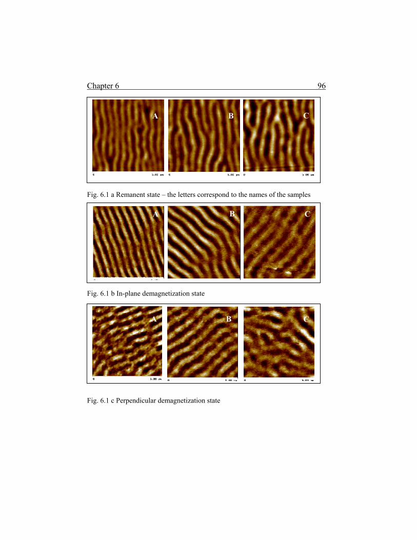
Chapter 6 96 Fig. 6.1 a Remanent state – the letters correspond to the names of the samples Fig. 6.1 b In-plane demagnetization state Fig. 6.1 c Perpendicular demagnetization state

A B C

A

A

B

B C

C

Chapter 6 97 Fig.6.2 Normalized hysteresis loops of Fe-Zr-N samples obtained by DC sputtering changing the input power, see Table 6.1 Table 6.1. Sample N

(at.%) P

(W) t

(nm) 4πMS (kG)

HS (Oe)

τ (nm)

ku (erg/cm3)

δ (nm)

A 7.6 3 500 18.3 440 220 4.3x105 62 B 6.3 5 460 19.4 175 280 2.1x105 85 C 5.7 7 480 19.4 100 315 1.4x105 103 D 4.3 9 440 19.6 - -

Characteristics of the samples versus nitrogen content. The symbols are explained in the text.

-600 -400 -200 0 200 400 600-1.0

-0.5

0.0

0.5

1.0

M/M

S

H (Oe)

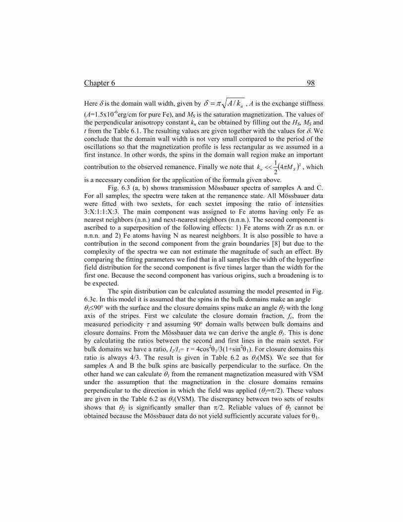
Chapter 6 98 Here δ is the domain wall width, given by ukA /πδ = , A is the exchange stiffness (A=1.5x10-6erg/cm for pure Fe), and MS is the saturation magnetization. The values of the perpendicular anisotropy constant ku can be obtained by filling out the HS, MS and t from the Table 6.1. The resulting values are given together with the values for δ. We conclude that the domain wall width is not very small compared to the period of the oscillations so that the magnetization profile is less rectangular as we assumed in a first instance. In other words, the spins in the domain wall region make an important

contribution to the observed remanence. Finally we note that ( )2421

Su Mk π<< , which

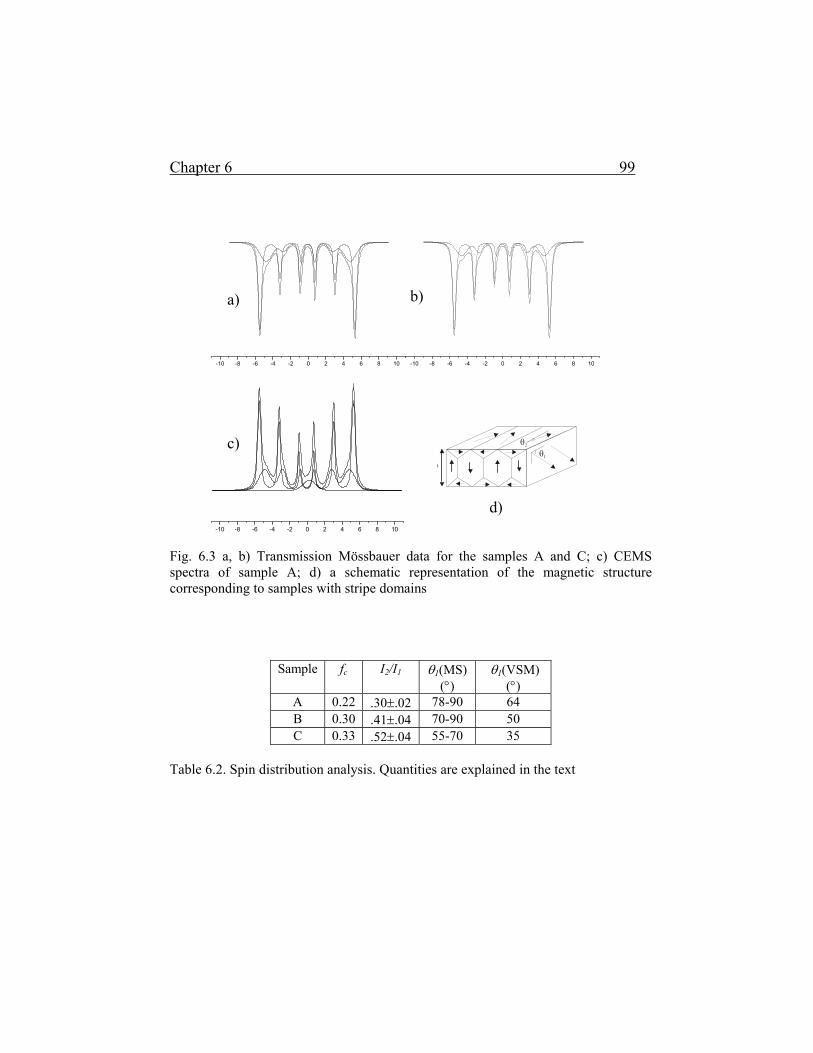
is a necessary condition for the application of the formula given above. Fig. 6.3 (a, b) shows transmission Mössbauer spectra of samples A and C.

For all samples, the spectra were taken at the remanence state. All Mössbauer data were fitted with two sextets, for each sextet imposing the ratio of intensities 3:X:1:1:X:3. The main component was assigned to Fe atoms having only Fe as nearest neighbors (n.n.) and next-nearest neighbors (n.n.n.). The second component is ascribed to a superposition of the following effects: 1) Fe atoms with Zr as n.n. or n.n.n. and 2) Fe atoms having N as nearest neighbors. It is also possible to have a contribution in the second component from the grain boundaries [8] but due to the complexity of the spectra we can not estimate the magnitude of such an effect. By comparing the fitting parameters we find that in all samples the width of the hyperfine field distribution for the second component is five times larger than the width for the first one. Because the second component has various origins, such a broadening is to be expected.

The spin distribution can be calculated assuming the model presented in Fig. 6.3c. In this model it is assumed that the spins in the bulk domains make an angle θ1≤90° with the surface and the closure domains spins make an angle θ2 with the long axis of the stripes. First we calculate the closure domain fraction, fc, from the measured periodicity τ and assuming 90° domain walls between bulk domains and closure domains. From the Mössbauer data we can derive the angle θ1. This is done by calculating the ratios between the second and first lines in the main sextet. For bulk domains we have a ratio, I2/I1= r = 4cos2θ1/3(1+sin2θ1). For closure domains this ratio is always 4/3. The result is given in Table 6.2 as θ1(MS). We see that for samples A and B the bulk spins are basically perpendicular to the surface. On the other hand we can calculate θ1 from the remanent magnetization measured with VSM under the assumption that the magnetization in the closure domains remains perpendicular to the direction in which the field was applied (θ2=π/2). These values are given in the Table 6.2 as θ1(VSM). The discrepancy between two sets of results shows that θ2 is significantly smaller than π/2. Reliable values of θ2 cannot be obtained because the Mössbauer data do not yield sufficiently accurate values for θ1.

Chapter 6 99

Fig. 6.3 a, b) Transmission Mössbauer data for the samples A and C; c) CEMS spectra of sample A; d) a schematic representation of the magnetic structure corresponding to samples with stripe domains

Sample fc I2/I1 θ1(MS) (°)

θ1(VSM) (°)

A 0.22 .30±.02 78-90 64 B 0.30 .41±.04 70-90 50 C 0.33 .52±.04 55-70 35

Table 6.2. Spin distribution analysis. Quantities are explained in the text

-10 -8 -6 -4 -2 0 2 4 6 8 10 -10 -8 -6 -4 -2 0 2 4 6 8 10

θ1

θ2

-10 -8 -6 -4 -2 0 2 4 6 8 10

a) b)

c)

d)

Chapter 6 100

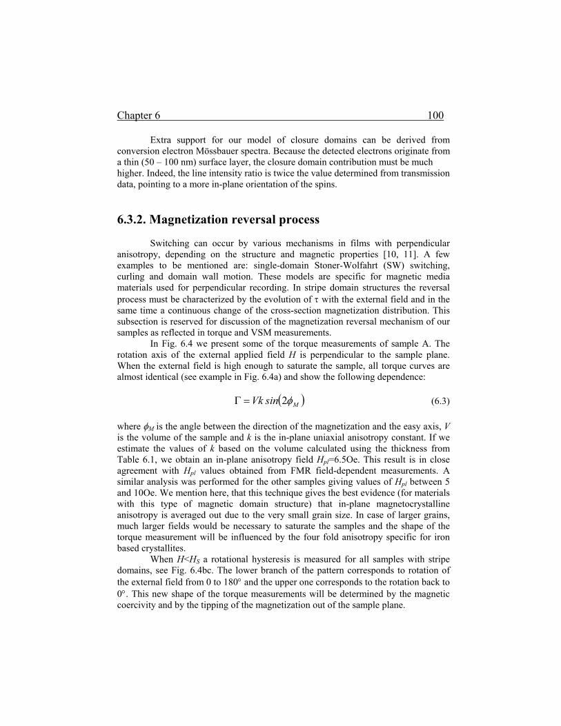
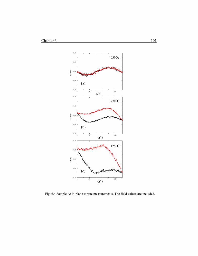
Extra support for our model of closure domains can be derived from conversion electron Mössbauer spectra. Because the detected electrons originate from a thin (50 – 100 nm) surface layer, the closure domain contribution must be much higher. Indeed, the line intensity ratio is twice the value determined from transmission data, pointing to a more in-plane orientation of the spins. 6.3.2. Magnetization reversal process Switching can occur by various mechanisms in films with perpendicular anisotropy, depending on the structure and magnetic properties [10, 11]. A few examples to be mentioned are: single-domain Stoner-Wolfahrt (SW) switching, curling and domain wall motion. These models are specific for magnetic media materials used for perpendicular recording. In stripe domain structures the reversal process must be characterized by the evolution of τ with the external field and in the same time a continuous change of the cross-section magnetization distribution. This subsection is reserved for discussion of the magnetization reversal mechanism of our samples as reflected in torque and VSM measurements. In Fig. 6.4 we present some of the torque measurements of sample A. The rotation axis of the external applied field H is perpendicular to the sample plane. When the external field is high enough to saturate the sample, all torque curves are almost identical (see example in Fig. 6.4a) and show the following dependence:

( )MsinVk φ2=Γ (6.3)

where φM is the angle between the direction of the magnetization and the easy axis, V is the volume of the sample and k is the in-plane uniaxial anisotropy constant. If we estimate the values of k based on the volume calculated using the thickness from Table 6.1, we obtain an in-plane anisotropy field Hpl=6.5Oe. This result is in close agreement with Hpl values obtained from FMR field-dependent measurements. A similar analysis was performed for the other samples giving values of Hpl between 5 and 10Oe. We mention here, that this technique gives the best evidence (for materials with this type of magnetic domain structure) that in-plane magnetocrystalline anisotropy is averaged out due to the very small grain size. In case of larger grains, much larger fields would be necessary to saturate the samples and the shape of the torque measurement will be influenced by the four fold anisotropy specific for iron based crystallites.

When H<HS a rotational hysteresis is measured for all samples with stripe domains, see Fig. 6.4bc. The lower branch of the pattern corresponds to rotation of the external field from 0 to 180° and the upper one corresponds to the rotation back to 0°. This new shape of the torque measurements will be determined by the magnetic coercivity and by the tipping of the magnetization out of the sample plane.

Chapter 6 101

Fig. 6.4 Sample A: in-plane torque measurements. The field values are included.

0 50 100 150-0.10

-0.05

0.00

0.05

0.10

Happl=50 kA/m

Γ(µN

m)

θ(O)

0 50 100 150-0.10

-0.05

0.00

0.05

0.10

Happl= 22 kA/m

Γ(µN

m)

θ(O)

0 50 100 150-0.10

-0.05

0.00

0.05

0.10

Happl=10 kA/m

Γ(µN

m)

θ(O)

(c)

(b)

(a)

630Oe

270Oe

125Oe

φ(°)

φ(°)

φ(°)

Chapter 6 102 Generally:

Γ=V[M||H sin(φM-φH)+k sin(2φM)] (6.4)

where φH is the angle made by H with respect to the in-plane anisotropy direction and M|| is the in-plane component of the magnetization. Although the torque due to the last term is still visible, the pattern is dominated by the frictional torque necessary to rotate the stripe domain pattern to a new position. This torque is associated with the first term in eq. (6.4). Starting from θ=0°, the angle ∆φ=(φM-φH) increases till the frictional torque becomes roughly constant. According to Fig. 6.4c, this happens when φH≅70° for H=250Oe. Rotating in the reverse direction this behavior repeats with the sign of the torque reversed.

The difference ∆φ shows up as a horizontal shift of the elastic part of the torque, which is measured as a function of φH. Inspection of Fig. 6.4b,c shows that ∆φ must be rather small. A reliable estimation for ∆φ in the interval [70°,180°] can be obtained by inserting the following parameters in equation 6.4: Γ(first term) = 0.7x10-4Nm, V=0.4x10-10m3, M||=0.5MS (from the VSM measurement), H=125Oe (Fig. 6.4c). We find sin∆φ=0.18, so ∆φ≅10°. For the torque measured at 270Oe, we find in the same way ∆φ=9°.

Combining the results from the in-plane torque measurements and the hysteresis loops, we obtain the following reversal mechanism of the magnetization: i) when H<HS the stripes start to form along the H direction and θ1 increases with the decrease of H, ii) the in-plane switching of the magnetization is realized when θ1 reaches a critical value and the magnetic system rotates very fast from φH-φM=180° to φH-φM=0°. Very close values of |M/MS| are recorded before and after switching. The mechanism proposed here has to be considered in the interpretation of others types of measurements like anisotropic magnetoresistance of similar samples [12, 13].

In Fig. 6.5a,b we present perpendicular torque measurements on sample A. The rotation axis of the field H⊥ is in the sample plane and perpendicular to the in- plane easy axis. Because the shape anisotropy is much bigger than ku, when H⊥ is close to the saturation value the magnetic system will rotate almost coherently. Although a very small rotational hysteresis loss is observed in all Γ(θ) curves with H⊥ smaller than the saturation value, a significant change in shape can be observed only at low fields, starting with H⊥=1.9kOe. The field angles θ0 where the switching takes place versus H⊥ are plotted in Fig. 6.5c. These angles correspond to the out-of plane direction of the average magnetization, for which the torque values are zero [13]. It can be seen that when H⊥ decreases to 0 the switching angle increases towards the value specific for the magnetization at remanence corresponding to the in-plane hysteresis loops. Since the values of H⊥ corresponding to the onset of stripe domain structure are given by the angle between magnetization and the field, as well as the

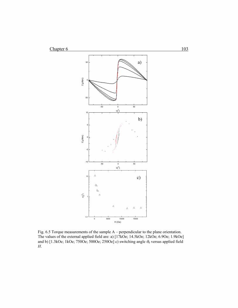
Chapter 6 103

Fig. 6.5 Torque measurements of the sample A – perpendicular to the plane orientation. The values of the external applied field are: a) [17kOe; 14.5kOe; 12kOe; 6.9Oe; 1.9kOe] and b) [1.3kOe; 1kOe; 750Oe; 500Oe; 250Oe] c) switching angle θ0 versus applied field H.

-50 0 50

-50

0

50

Γ(µ

Nm

)

θ(0)

-50 0 50-10

-5

0

5

10

Γ(µ

Nm

)

θ(O)

0 5000 10000 150000.1

1

10

θ 0(0 )

H (Oe)

a)

b)

c)

Chapter 6 104 field magnitude, H⊥= H⊥( θ0) can be much larger than HS (the saturation field for the in-plane geometry) . We do not exclude that when the external field is perpendicular to the sample plane the stripe domains can form for all fields smaller than the value required for the saturation of the sample.

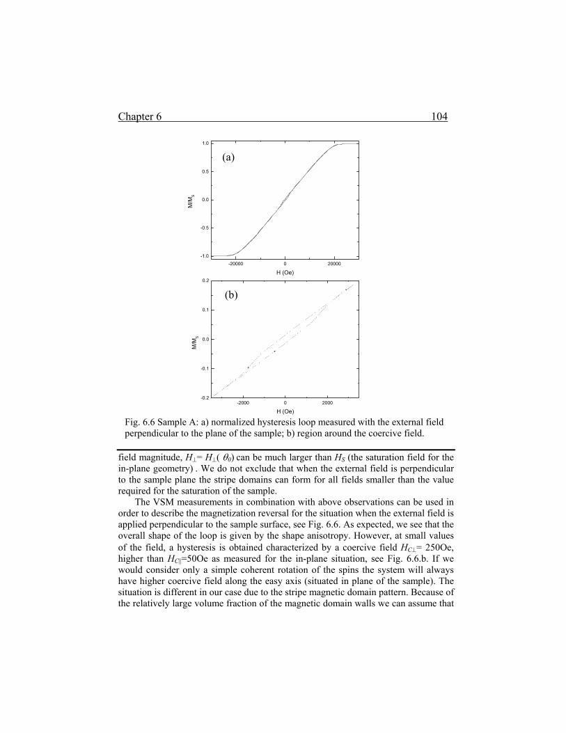
The VSM measurements in combination with above observations can be used in order to describe the magnetization reversal for the situation when the external field is applied perpendicular to the sample surface, see Fig. 6.6. As expected, we see that the overall shape of the loop is given by the shape anisotropy. However, at small values of the field, a hysteresis is obtained characterized by a coercive field HC⊥= 250Oe, higher than HC||=50Oe as measured for the in-plane situation, see Fig. 6.6.b. If we would consider only a simple coherent rotation of the spins the system will always have higher coercive field along the easy axis (situated in plane of the sample). The situation is different in our case due to the stripe magnetic domain pattern. Because of the relatively large volume fraction of the magnetic domain walls we can assume that

Fig. 6.6 Sample A: a) normalized hysteresis loop measured with the external field perpendicular to the plane of the sample; b) region around the coercive field.

-20000 0 20000-1.0

-0.5

0.0

0.5

1.0

M/M

S

H (Oe)

-2000 0 2000-0.2

-0.1

0.0

0.1

0.2

M/M

S

H (Oe)

(a)

(b)

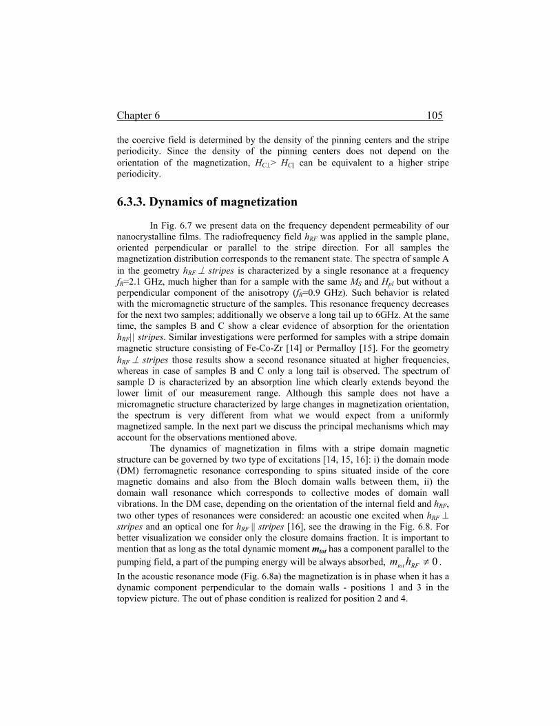
Chapter 6 105 the coercive field is determined by the density of the pinning centers and the stripe periodicity. Since the density of the pinning centers does not depend on the orientation of the magnetization, HC⊥> HC|| can be equivalent to a higher stripe periodicity. 6.3.3. Dynamics of magnetization In Fig. 6.7 we present data on the frequency dependent permeability of our nanocrystalline films. The radiofrequency field hRF was applied in the sample plane, oriented perpendicular or parallel to the stripe direction. For all samples the magnetization distribution corresponds to the remanent state. The spectra of sample A in the geometry hRF ⊥ stripes is characterized by a single resonance at a frequency fR=2.1 GHz, much higher than for a sample with the same MS and Hpl but without a perpendicular component of the anisotropy (fR=0.9 GHz). Such behavior is related with the micromagnetic structure of the samples. This resonance frequency decreases for the next two samples; additionally we observe a long tail up to 6GHz. At the same time, the samples B and C show a clear evidence of absorption for the orientation hRF|| stripes. Similar investigations were performed for samples with a stripe domain magnetic structure consisting of Fe-Co-Zr [14] or Permalloy [15]. For the geometry hRF ⊥ stripes those results show a second resonance situated at higher frequencies, whereas in case of samples B and C only a long tail is observed. The spectrum of sample D is characterized by an absorption line which clearly extends beyond the lower limit of our measurement range. Although this sample does not have a micromagnetic structure characterized by large changes in magnetization orientation, the spectrum is very different from what we would expect from a uniformly magnetized sample. In the next part we discuss the principal mechanisms which may account for the observations mentioned above.

The dynamics of magnetization in films with a stripe domain magnetic structure can be governed by two type of excitations [14, 15, 16]: i) the domain mode (DM) ferromagnetic resonance corresponding to spins situated inside of the core magnetic domains and also from the Bloch domain walls between them, ii) the domain wall resonance which corresponds to collective modes of domain wall vibrations. In the DM case, depending on the orientation of the internal field and hRF, two other types of resonances were considered: an acoustic one excited when hRF ⊥ stripes and an optical one for hRF || stripes [16], see the drawing in the Fig. 6.8. For better visualization we consider only the closure domains fraction. It is important to mention that as long as the total dynamic moment mtot has a component parallel to the pumping field, a part of the pumping energy will be always absorbed, 0≠RFtot hm . In the acoustic resonance mode (Fig. 6.8a) the magnetization is in phase when it has a dynamic component perpendicular to the domain walls - positions 1 and 3 in the topview picture. The out of phase condition is realized for position 2 and 4.

Chapter 6 106

Fig. 6.7 Permeability spectra - samples A, B, C and D. Left columncorresponds to HRF⊥ stripes and right column corresponds to HRF|| stripes.

A A

B B

C C

D D

-1000

0

1000

2000

-1000

0

1000

2000

-1000

0

1000

2000

3000

-1000

0

1000

2000

3000

-1000

0

1000

2000

3000

0.00E+000 2.00E+009 4.00E+009 6.00E+009

0

2000

4000

6000

8000

Frequency (Hz)

0.00E+000 2.00E+009 4.00E+009 6.00E+009

0

2000

4000

6000

8000

Frequency (Hz)

-1000

0

1000

2000

3000

Chapter 6 107

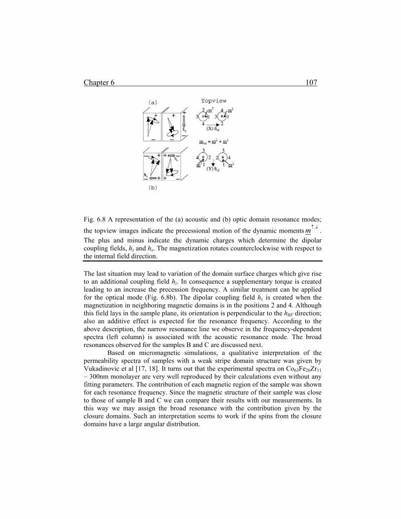
Fig. 6.8 A representation of the (a) acoustic and (b) optic domain resonance modes;

the topview images indicate the precessional motion of the dynamic moments ↓↑ ,m . The plus and minus indicate the dynamic charges which determine the dipolar coupling fields, hz and hx. The magnetization rotates counterclockwise with respect to the internal field direction.

The last situation may lead to variation of the domain surface charges which give rise to an additional coupling field hz. In consequence a supplementary torque is created leading to an increase the precession frequency. A similar treatment can be applied for the optical mode (Fig. 6.8b). The dipolar coupling field hx is created when the magnetization in neighboring magnetic domains is in the positions 2 and 4. Although this field lays in the sample plane, its orientation is perpendicular to the hRF direction; also an additive effect is expected for the resonance frequency. According to the above description, the narrow resonance line we observe in the frequency-dependent spectra (left column) is associated with the acoustic resonance mode. The broad resonances observed for the samples B and C are discussed next. Based on micromagnetic simulations, a qualitative interpretation of the permeability spectra of samples with a weak stripe domain structure was given by Vukadinovic et al [17, 18]. It turns out that the experimental spectra on Co63Fe26Zr11 – 300nm monolayer are very well reproduced by their calculations even without any fitting parameters. The contribution of each magnetic region of the sample was shown for each resonance frequency. Since the magnetic structure of their sample was close to those of sample B and C we can compare their results with our measurements. In this way we may assign the broad resonance with the contribution given by the closure domains. Such an interpretation seems to work if the spins from the closure domains have a large angular distribution.

Chapter 6 108

In the hRF || stripes geometry the resonance attributed to spins inside of the core magnetic domains corresponds to the optical domain resonance mode; additionally closure domains may also give a resonance at higher frequencies (compare the modes (4) and (5) in Ref. [17] with the corresponding spectra of samples B and C). However, in this geometry the intensity of the resonances is one order of magnitude smaller than for the other geometry. This is reflected in the experimental data. In view of the limited precision we do not discuss them in any detail. 6.4. Conclusions

We have studied Fe-Zr-N thin films with a dense stripe magnetic domain structure. A continuous transition to in-plane spin orientation was observed in films with the same thickness and a variable composition. The sample without stripe magnetic domains has a small coercive field and high saturation magnetization.

By combining magnetic force microscopy, VSM measurements and Mössbauer spectroscopy we have detected the spin distribution perpendicular to the plane of the sample. This method can be used as an alternative to the much more “expensive” investigations using x-ray resonant magnetic scattering [9], for samples with a thickness from a few nanometers to one micrometer. The stripe domain structure has a magnetization reversal mechanism which consists of two separate rotation processes. First the spins in the stripe domains turn out of the plane. When the out of plane angle θ1 reaches a critical value θ1C the entire spin pattern rotates 180° keeping the average magnetization in plane of the sample.

We have proven that the materials with stripe domain magnetic structure are potential candidates for high frequency applications. The sample with the highest perpendicular anisotropy has a high initial permeability, a FMR frequency higher than 2 GHz and a linewidth of 500MHz. These properties are adjusted by changing the perpendicular anisotropy component via nitrogen concentration. Depending on the micromagnetic structure the permeability spectra show the influence of the different magnetic regions in the sample.

Chapter 6 109 References

1. L. Klein, Y. Kats, A.F. Marshall, J.W. Reiner, T.H. Geballe, M.R. Beasley, and A. Kapitulnik, Phys.Rev.Lett. 84, 6090 (2000), and therein references

2. Y. Murayama, J.Phys.Soc.Japan, vol 21, No.11, 2253 (1966) 3. L.M. Alvarez-Prado, G.T. Pérez, R. Morales, F.H. Salas, and J.M. Alameda,

Phys.Rev.B. 56, 3306 (1997), and theirs references 4. A.Marty, Y.Samson, B. Gilles, M. Belakhovsky, E. Dudzik, H.Dürr, S.S.

Dhesi, G. van der Laan, J.B. Goedkoop, J.Appl.Phys., Vol. 87, No.9, 5472 (2000)

5. A. Hubert and R. Schäfer, Magnetic domains, Springer-Verlag Berlin Heidelberg New-York, (2000)

6. M. Labrune anf J. Miltat, J. Appl. Phys. 75, 2156, (1994) 7. K.H. Kim, Y.K. Kim, J. Kim, S.H. Han, H.J. Kim, J. Magn. Magn. Mater.

215-216, 368 (2000) 8. J.Balogh, L.Bujdosó, D.Kaptas, and T. Kemény, I. Vincze, S. Szabó, and

D.L. Beke, Phys. Rev. B 61, 4109 (2000) 9. E. Dudzik, S.S. Dhesi, H.A. Dürr, S.P. Collins, M.D. Roper, G. van der Laan,

K. Chesnel, M. Belakhovsky, and Y. Samson, Phys. Rev. B 62, 5779 (2000) 10. Y. Ishii, S. Hasegawa, M. Saito, Y. Tabayashi, Y. Kasajima, and T.

Hashimoto, J. Appl. Phys. 82, 3593 (1997) 11. G. T. A. Huysmans, J. C. Lodder, and J. Walkui, J. Appl. Phys. 64, 2016

(1988) 12. N. Saito, H. Fujiwara, and Y. Sugita, J. Phys. Soc. Jap. 19, 1116 (1964) 13. U. Rüdiger, J. Yu, L. Thomas, S. S. P. Parkin, and A. D. Kent, Phys. Rev. B

59,11914 (1999). 14. O. Acher, C. Boscher, B. Brule, and G. Perrin, J. Appl. Phys. 81, 4057

(1997) 15. E. Moriatakis, L. Kompotiatis, M. Pissas, D. Niarcos, J. Magn. Magn. Mater.

222, 168 (2000). 16. U. Ebels, P. E. Wingen, and K. Ounadjela, J. Magn. Magn. Mater. 177-181,

1239 (1998) 17. N. Vukadinovic, O. Vacus, M. Labrune, O. Acher, and D. Pain, Phys. Rev.

Lett. 85, 2817 (2000) 18. N. Vukadinovic, M. Labrune, J. Ben Youssef, A. Marty, J.C. Toussaint, and

H. Le Gall, Phys. Rev.B 65, 054403 (2001).

Chapter 6 110