university of groningen forecasting in planning ike, p
TRANSCRIPT

University of Groningen
Forecasting in PlanningIke, P.; Voogd, Henk
Published in:Environmental and Infrastructure Planning
IMPORTANT NOTE: You are advised to consult the publisher's version (publisher's PDF) if you wish to cite fromit. Please check the document version below.
Document VersionPublisher's PDF, also known as Version of record
Publication date:2004
Link to publication in University of Groningen/UMCG research database
Citation for published version (APA):Ike, P., & Voogd, H. (2004). Forecasting in Planning. In H. Voogd, & G. Linden (Eds.), Environmental andInfrastructure Planning (pp. 157 - 182). Geo Press.
CopyrightOther than for strictly personal use, it is not permitted to download or to forward/distribute the text or part of it without the consent of theauthor(s) and/or copyright holder(s), unless the work is under an open content license (like Creative Commons).
The publication may also be distributed here under the terms of Article 25fa of the Dutch Copyright Act, indicated by the “Taverne” license.More information can be found on the University of Groningen website: https://www.rug.nl/library/open-access/self-archiving-pure/taverne-amendment.
Take-down policyIf you believe that this document breaches copyright please contact us providing details, and we will remove access to the work immediatelyand investigate your claim.
Downloaded from the University of Groningen/UMCG research database (Pure): http://www.rug.nl/research/portal. For technical reasons thenumber of authors shown on this cover page is limited to 10 maximum.
Download date: 27-01-2022

Environmental and Infrastructure Planning 157
9 Forecasting in planning
Paul Ike and Henk Voogd
1 Introduction
Planning is concerned with a deliberate set of actions aimed at
improvements in future qualities that would not otherwise be realized
within a given time. This description indicates that ‘the future’ is a key
concept in planning. However, the word ‘qualities’ also implies that the
future is not an objective reality but rather a subjective construction.
Evidently, each person has his or her own interpretation of the meaning
of ‘good quality’. A forecast is a statement about future conditions and
therefore is always arbitrary, rather than being ‘a statement of fact’.
The term ‘forecasting’ is often used for both quantitative predictions of
future developments and for qualitative explorations of possible futures
(Armstrong, 1985; Makridakis et al., 1998; Pourahmadi, 2001). In this
paper we will discuss both types of forecasts and their use in
environmental and infrastructure planning.
2 Qualitative forecasting
Qualitative forecasting methods principally rely on personal judgements
to generate forecasts. These methods consist of guidelines or procedures
for gathering the opinions of experts, stakeholders or other interested
parties. Qualitative methods can be used when one or more of the
following conditions occur:
158 Paul Ike and Henk Voogd
There is little or no historical data on the variables to be forecast
The relevant environment is likely to be unstable during the
forecast horizon
The forecast has a long time horizon, that is, five years or more.
The two most popular qualitative approaches will be briefly discussed
here: the ‘Delphi method’ and the ‘Scenario’ approach.
2.1 Delphi method
An interactively structured collection of anonymous opinions is often
called a Delphi method (Sackman, 1975; Kenis, 1995). The anonymous
exchange of opinions is the most important characteristic of a Delphi
approach, as in a group setting opinions can be influenced by many
things, including the dominant positions of some participants, personal
characteristics and ‘alleged expertise’. It is less meaningful to strive for a
consensus forecast by just putting all the experts in a room and letting
them ‘argue it out’. This method falls short because those individuals
with the best group interaction and persuasion skills often control the
situation.
The Delphi method was originally developed in the 1950s by the
RAND Corporation, a US Intelligence think tank. It had its greatest
triumphs in the 1960s and 1970s (Linstone and Turoff, 1975). However,
in the last decade we have seen a strong revival due to, among others
reasons, modern computer techniques for organizing such brainstorming
sessions in a network setting, so-called ‘groupware’. At present, many
consulting firms have their own approach to structured brainstorming
and, of course, their own ‘trade name’. Evidently, recent interest in
collaborative approaches and consensus planning is another important
reason for the application of this method (Woltjer, 2000).
The basic structure of a procedure according to the Delphi
method is as follows:
1. The selection of participants.
2. An initial set of questions sent to all participants. For example, in the
case of a forecast they can be asked for estimates of certain variables at a
future time, for the likelihood that these estimates will be realized, for
minimum and maximum estimates, and last but not least, the reasons for
these estimates.
3. The co-ordinator, or computer program, then tabulates or summarizes
the outcomes into, for example, expected or average figures.
4. Results are then returned to each participant along with anonymous
statements and they are asked to review their earlier opinion.

Environmental and Infrastructure Planning 159
5. The process continues until little or no change occurs. The end result
may then be seen as a consensus solution.
A strong point of this approach is that it can be applied under
many circumstances since it is not strictly dependent on a priori
information. A brief fact sheet, a long report or a presentation of the
problem under consideration may, of course, benefit the thinking of
participants, but the original idea is that each participant enters the
procedure with only his or her own basic knowledge. The process of the
group creation of judgmental forecasts is largely one of reasoning and
argumentation. These reasons and justifications underpinning the
forecast may be crucial in persuading outsiders to accept the outcomes.
A weak point is that the final result will always depend on the people
who are invited to participate, on their ability to think along the lines
required and to express themselves clearly. Also, a consensus solution
may give a false idea of ‘certainty’, but in planning, ‘consensus’ usually
has a much higher priority than attempting to predict certainty in a future
that is intrinsically uncertain.
2.2 Scenario approach
Wiener and Kahn (1967) introduced the notion ‘scenario’ in their book
‘The Year 2000’. A scenario is a narrative forecast that describes a
potential course of events. It should recognize the interrelationships of
system components. A scenario is a "script" for defining a possible
future including likely impacts on the other components and the system
as a whole.
I II III
Figure 1. Scenarios describe the present situation (I) and possible future
situations (III) and a plausible route between both (II)
Scenarios are written as long-term predictions of the future. A proper
scenario involves a description of a future situation (III in Figure 1) and
the course of events (II) that enables a system to move forward from the

160 Paul Ike and Henk Voogd
original situation (I) to the future situation (III). Scenarios often consider
events such as new technology, population shifts, changing economic
situations, for example, regarding consumer preferences, and different
levels of government involvement, for example through investments.
The primary purpose of a scenario is to provoke thinking of
policymakers who can then posture themselves for the fulfilment of the
scenario(s). A most likely scenario is usually written, along with at least
one optimistic and one pessimistic scenario, but of course other
assumptions can also be used as leading motive.
Two major types of scenario are often identified:
- Projective scenarios (sometimes also called exploratory
scenarios): starting from past and present trends and leading to a
likely future;
- Prospective scenarios (or anticipatory or normative scenarios):
built on the basis of different visions of the future that may be
desired or, on the contrary, feared.

Environmental and Infrastructure Planning 161
(adapted from Coates, 1996)
Figure 2. Example of an integrated scenario-working scheme

162 Paul Ike and Henk Voogd
Source: Das et al (1966)
Figure 3. A 1966 view on the future of Amsterdam in 2000
The preparation of a prospective scenario is also known as backcasting
(Dreborg, 1996). It involves working backward from a particular
desirable future endpoint to determine the physical feasibility of that
future and what policy measures would be required to reach it (see for
examples: Hojer, 1998). In Figure 2 an integrated working scheme is

Environmental and Infrastructure Planning 163
outlined that includes both a prospective and projective approach. This
scheme is robust, i.e. it can be combined both with a Delphi-approach
and with quantitative forecasting.
Visions of the future are of course very speculative, but very
interesting for the exploration of new avenues of thought. See for
example Figure 3, which is borrowed from a 1966 book on urban
planning (Das et al., 1966). It shows a number of developments that are
still ‘futuristic’ today, after 2000. For instance, the public resistance
against demolition of houses for new developments has clearly been
underestimated.
2.3 An example: Transit-Oriented Development
The Scenario approach can combine very well with the Delphi method.
An example, borrowed from Nelson and Niles (2000), will be briefly
summarized here. It concerns a study of a transit-oriented development
(TOD). This is a mix of shopping, service, and recreational activities at
urban centres linked together by a high quality transit system that
induces citizens to drive less and to walk and use the transit system more
often. Transit-Oriented Development (TOD) has rapidly emerged as the
central urban planning paradigm in the United States. Leaders in many
metropolitan areas have made, or are contemplating making, major
investments in new rail transit capacity under the assumption that
synergy between compact, mixed-use development and mass transit will
change car-dependent growth and travel patterns.
The success of the TOD concept (Figure 4) depends greatly on
the response of developers, consumers, and other economic actors to the
new land use-transportation configuration. This has been a reason for
applying a combined Delphi-Scenario method to learn more about
potential effects. A multidisciplinary panel was created that included
urban planners, architects, urban geographers, urban economists,
commercial developers, store site selection managers, transportation
planners, and environmental organization representatives.
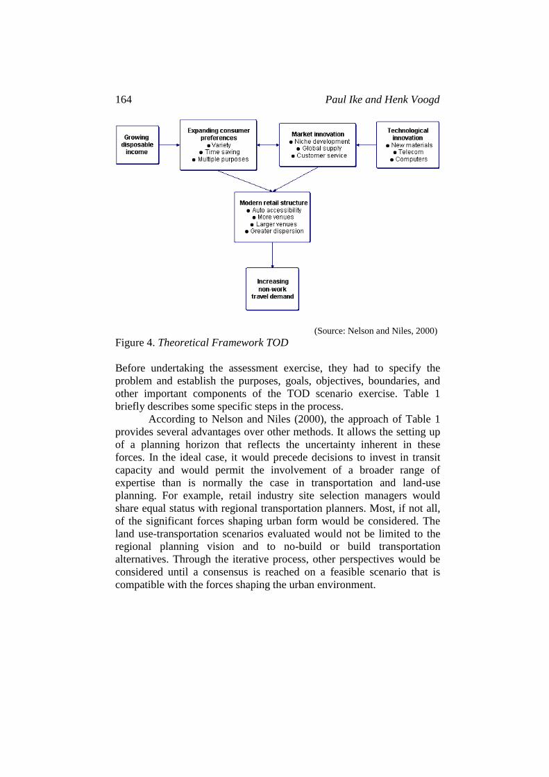
164 Paul Ike and Henk Voogd
(Source: Nelson and Niles, 2000)
Figure 4. Theoretical Framework TOD
Before undertaking the assessment exercise, they had to specify the
problem and establish the purposes, goals, objectives, boundaries, and
other important components of the TOD scenario exercise. Table 1
briefly describes some specific steps in the process.
According to Nelson and Niles (2000), the approach of Table 1
provides several advantages over other methods. It allows the setting up
of a planning horizon that reflects the uncertainty inherent in these
forces. In the ideal case, it would precede decisions to invest in transit
capacity and would permit the involvement of a broader range of
expertise than is normally the case in transportation and land-use
planning. For example, retail industry site selection managers would
share equal status with regional transportation planners. Most, if not all,
of the significant forces shaping urban form would be considered. The
land use-transportation scenarios evaluated would not be limited to the
regional planning vision and to no-build or build transportation
alternatives. Through the iterative process, other perspectives would be
considered until a consensus is reached on a feasible scenario that is
compatible with the forces shaping the urban environment.

Environmental and Infrastructure Planning 165
Step Scope
Describe present retail
structure/patterns
Present urban structure including retail market,
travel patterns, past trends
Identify forces shaping
urban form
Understanding and subjective weighting of
forces: economic, environmental, social, and
technological. Focus on current and future market
trends: commercial development, consumer
behaviour, non-work travel patterns
Specify TOD scenario Likely station-area locations and types
(residential, retail, employment, mixed)
Specify transit system Size and quality of transit afforded under fiscal
constraints
Define success Economic, societal, personal, and environmental
benefits and costs; elaborate 16 planning factors;
establish planning horizon
Evaluate success Identification of constraints and supporting
policies to achieve feasibility; adaptation to new
knowledge and consideration of alternative
solutions as needed
(Source: Nelson and Niles, 2000)
Table 1. Stages in Delphi-scenario approach for TOD
With a multi-disciplinary Delphi panel, broader social equity questions
would also likely be considered, as well as a range of opportunity costs.
The process can be open to the public in ways that quantitative
forecasting cannot be. The empirical data, estimates, and assumptions
would be available for public inspection. A report might be issued after
each step, which would allow stakeholders, including elected officials,
the opportunity to provide feedback throughout the effort. Information
considered and techniques used would be transferable across regions.
3 Quantitative forecasting
Quantitative forecasting methods use numerical empirical data to
forecast the future. The objective of these methods is to study past events
in order to understand the underlying structure of the data and use that
knowledge to predict future occurrences. Quantitative methods can be
used in planning when one or more of the following conditions occur:

166 Paul Ike and Henk Voogd
A sufficient and consistent set of historical data on the
variables to be forecast
The likely stability of the relevant environment during the
forecast horizon
The forecast has a short time horizon, that is, five years or
less.
The two most popular quantitative approaches will be briefly discussed
here: ‘Time series’ forecasting, which involves projecting future values
of a variable based on past and current observations of the variable
(Pourahmadi, 2001; Chatfield, 1996; Weigend and Gershenfeld, 1994;
Box and Jenkins, 1970) and ‘Causal’ forecasting, which involves finding
factors that relate to the variable being predicted and using those factors
to predict future values of the variable (Makridakis et al., 1998;
Morrison, 1991; Wyatt, 1989; Anas, 1987; Wesolowsky, 1976).
3.1 Time series methods
A times series refers to data which is ordered according to the time of
collection, usually spaced at equal intervals such as years. A planner is
sometimes involved in a process whereby a forecast is needed for a
variable with an unknown theoretical relationship to other predicting
variables, for example, due to a lack of data. For instance, times series
methods may be appropriate for forecasting in such cases as price
developments over time in some sectors of real estate. Three specific
time series methods are:
Moving average
Exponential smoothing
Least squares trend analysis
The ‘moving average’ method is one of the simplest methods of
forecasting. It assumes that a future value will equal an average of past
values. The moving average method uses an average of a number of
prior periods to forecast the next period. If a 2-period moving average is
calculated, the average for the two prior periods is used as the forecast
for the third period.
‘Exponential smoothing’ is a technique for averaging current and past
observations in a time series. The procedure is based on a period-by-
period adjustment of the latest smoothed average. Single exponential
smoothing models require three items of data:
The most recent forecast
The most recent actual value
A smoothing constant

Environmental and Infrastructure Planning 167
The smoothing constant or ‘damping factor’ (w) determines the weights
given to the most recent past observations and, therefore, controls the
rate of smoothing or averaging. The constant’s value must be between
zero and one. The equation for the exponential smoothing model is:
(1) Ft = wAt – 1 + (1 - w)Ft – 1
Where: Ft = exponentially smoothed forecast for period ‘t’
At – 1 = actual value in prior period
F t – 1 = exponentially smoothed forecast for prior period
w = smoothing constant or weight
To begin using the exponential smoothing method, the first actual value
is usually chosen as the forecast value for the second period. The lower
the smoothing factor is, the higher the importance attached to the most
recent data (see Figure 5).
Figure 5. Influence of smoothing factor
The least squares method can also be used to determine the trend line.
The method involves fitting a linear trend line through time-series data to
obtain an equation for a line of the form:
(2) Yt = b0 + b1Xt
Where: Yt = forecast value for time t
Xt = year
b0 = intercept of the trend line with the vertical axis, and
0
0.2
0.4
0.6
0.8
1
1 2 3 4 5 6
Periods Back
We
igh
t w = 0.500
w = 0.667
w = 0.900

168 Paul Ike and Henk Voogd
b1 = slope of the trend line
The least squares technique means that the line is fitted so that
the squared deviations between the predicted (forecasted) values and the
actual values are minimized. Regression analysis is used to determine the
trend line, whereby the years are the independent variable.
By using the least squares method also other functions than a
straight line can be fitted to the data. Options include logarithmic,
polynomial, power, and exponential functions.
Figure 6. Decomposition of a data pattern
A forecast can be improved if the underlying factors of a data pattern can
be identified and forecasted separately (e.g. see Figure 6). Breaking
down the data into its component parts is called decomposition. For
example, it can be assumed that housing sales are affected by four
factors: the general trend in the data, general economic cycles,
seasonality, and irregular or random occurrences. Considering each of
these components separately and then combining them together makes
the forecast.
A well-known forecasting method is ARIMA (Autoregressive
Integrated Moving Average), also known as the Box-Jenkins approach.
This method uses auto regression, differencing, and moving averages to
estimate time series variables. Auto regression is the relationship of
each value in a series to previous values. Differencing looks at the
changes from one observation to the next and is used to stabilize a time
series that seems to vary erratically. In a moving average process each
value is determined by the average value of the current disturbance and
one or more previous disturbances; a disturbance affects the value of the
Environmental and Infrastructure Planning 169
dependant variable for a finite number of periods and then abruptly
ceases to affect it. Specialized computer software is necessary to use the
ARIMA forecasting method and it requires a large amount of data,
which is seldom available in spatial planning settings.
3.2 Causal forecasting
Causal methods search for factors that relate to the variable being
predicted. Those factors are then used to predict future values of the
variable. Causal methods include:
Multiple regression analysis
Econometric models
Simulation models.
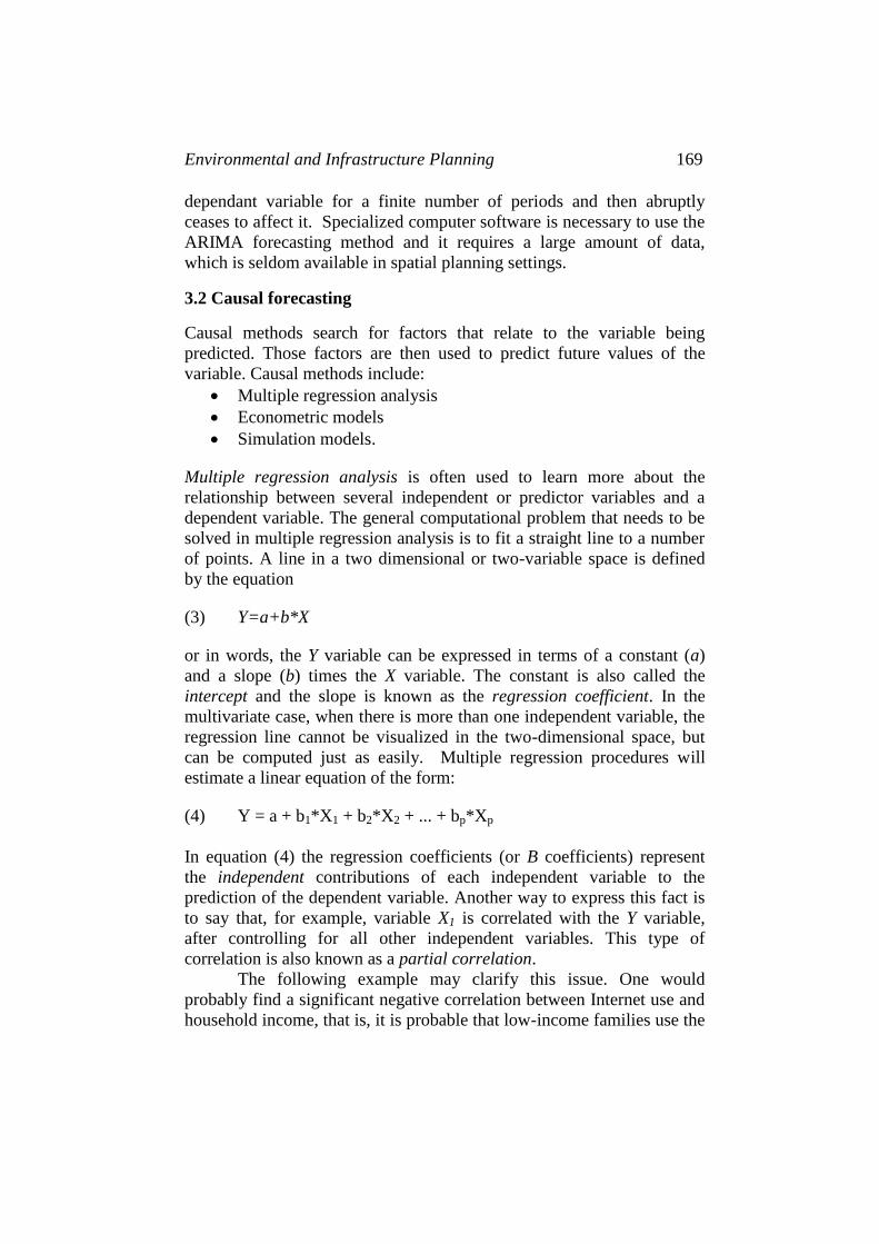
Multiple regression analysis is often used to learn more about the
relationship between several independent or predictor variables and a
dependent variable. The general computational problem that needs to be
solved in multiple regression analysis is to fit a straight line to a number
of points. A line in a two dimensional or two-variable space is defined
by the equation
(3) Y=a+b*X
or in words, the Y variable can be expressed in terms of a constant (a)
and a slope (b) times the X variable. The constant is also called the
intercept and the slope is known as the regression coefficient. In the
multivariate case, when there is more than one independent variable, the
regression line cannot be visualized in the two-dimensional space, but
can be computed just as easily. Multiple regression procedures will
estimate a linear equation of the form:
(4) Y = a + b1*X1 + b2*X2 + ... + bp*Xp
In equation (4) the regression coefficients (or B coefficients) represent
the independent contributions of each independent variable to the
prediction of the dependent variable. Another way to express this fact is
to say that, for example, variable X1 is correlated with the Y variable,
after controlling for all other independent variables. This type of
correlation is also known as a partial correlation.
The following example may clarify this issue. One would
probably find a significant negative correlation between Internet use and
household income, that is, it is probable that low-income families use the

170 Paul Ike and Henk Voogd
Internet more frequently. At first this may seem odd; however, if we
were to add the variable ‘level of urbanization’ into the multiple
regression equation, this correlation would probably disappear. This is
because in cities, on average, people have better Internet infrastructure
and facilities, for example, access to broadband cable and ADSL, but
low-income families also tend to be concentrated in cities. Thus, after we
remove this geographical difference by entering the urbanization level
into the equation, the relationship between household income and
Internet use disappears because household income does not make any
unique contribution to the prediction of Internet use, above and beyond
what it shares in the prediction with variable urbanization level. Put
another way, after controlling for the variable urbanization level, the
partial correlation between income and use of the Internet is zero.
The regression line expresses the best prediction of the dependent
variable (Y), given the independent variables (X). However, reality is
rarely (if ever) perfectly predictable, and usually there is substantial
variation of the observed points around the fitted regression line. The
deviation of a particular point from the regression line (its predicted
value) is called the residual value. The smaller the variability of the
residual values around the regression line relative to the overall
variability, the better is our prediction. If there is no relationship between
the X and Y variables, then the ratio of the residual variability of the Y
variable to the original variance is equal to 1.0. However, if X and Y are
perfectly related then there is no residual variance and the ratio of
variance would be 0.0. Usually the ratio falls somewhere between these
extremes, that is, between 0.0 and 1.0. 1.0 minus this ratio is referred to
as R-square or the coefficient of determination. This value is
immediately interpretable in the following manner. If we have an R-
square of 0.4 then we know that the variability of the Y values around
the regression line is 1-0.4 times the original variance; in other words we
have explained 40% of the original variability, and are left with 60%
residual variability. Ideally, we would like to explain most if not all of
the original variability. The R-square value is an indicator of how well
the model fits the data (e.g., an R-square close to 1.0 indicates that we
have accounted for almost all of the variability with the variables
specified in the model).
Usually, the degree to which two or more predictors (independent
or X variables) are related to the dependent (Y) variable is expressed in
the correlation coefficient R, which is the square root of R-square. In
multiple regression, R can assume values between 0 and 1. To interpret
the direction of the relationship between variables, one looks at the signs
(plus or minus) of the regression or B coefficients. If a B coefficient is

Environmental and Infrastructure Planning 171
positive, then the relationship of this variable with the dependent
variable is positive; if the B coefficient is negative then the relationship
is negative (e.g., the lower the income the higher the use of public
transport). Of course, if the B coefficient is equal to 0 then there is no
relationship between the variables.
Econometric models can be much more complex than a single multiple
regression equation. They are often made up of a hundred or possibly
many more equations, comparable to Equations 3 and 4. The basic
characteristic of proper econometric models is that the calibration of the
parameters and the reliability of the equations are empirically tested with
statistical measures. However, the aggregate prediction outcomes of
these models depend heavily on the quality of the data used and the
errors that are generated by the structure of the model itself. For
example, suppose variables A and B both have a value of 5 and an error
of +/- 1; the aggregate value of A and B is C. If C = A + B we have an
aggregate value between 4 + 4 = 8 and 6 + 6 = 12. In other words, the
aggregate value C has twice as much error than the original variables.
The amount of error considerably increases if a multiplicative
relationship is assumed, namely C = A·B. Now the aggregative value
varies between 16 and 36. In other words, C now has an error 10 times
that of the original variables! Clearly, this illustrates that the more
complex a mathematical model is, the more unreliable its outcomes are.
The same conclusion applies to ‘simulation models’. Forester has been
an important promoter of these models (Forester, 1961, 1971), which
focus on a formal representation of processes. The main difference they
have with econometric models is that the coefficients of a simulation
model have a physical significance and are measured directly or
determined by trial and error, that is, they are not deduced statistically.
Hence, the ‘plausibility’ of the outcome is an important criterion for
judging the usefulness of a simulation model.
3.3 An example: forecasting demand for sand
Causal forecasting will be illustrated by summarizing the Dutch history
of forecasting the future use of aggregates. The production of building
materials such as gravel, sand and clay usually involves the removal of
considerable amounts of the land surface, often near rivers. In addition,
in Europe materials such as hard rock and limestone are extracted from
pits. However, local policymakers and the surrounding population
usually do not appreciate this kind of ‘destructive’ land use. It is a clear

172 Paul Ike and Henk Voogd
example of a ‘not-in-my-backyard’ activity. For this reason, in several
European countries the forecasting of demand is used to show opponents
of mining that the building materials really are needed. The
policymakers concerned use the forecasts to legitimise the provision of
mineral permits, that is, the amount of land that is permitted for mineral
extraction depends on the forecasted future demand for that particular
building material. A multiple regression analysis is used as a forecasting
technique both in the Netherlands and other European countries (Lehoc,
1979; Bundesamt für Bauwesen und Raumordnung, 1998; EIB, 2002;
Department of the Environment, 1994).
This will be illustrated below with a chronological overview of
the way regression models for concrete and masonry sand have been
made in the Netherlands. Through the presentation of these models, the
use of regression analysis will be explained (Ike, 2000).
Concrete and masonry sand, i.e. coarse sand, is considered to be a scarce
building material in the Netherlands. This is not because of limited
geological availability, but instead to limited ‘land use planning’
availability. The annual demand varies between 18.5 and 24.5 million
tons per year. There has always been a problem accommodating this
demand with sufficient supply. Since 1975, models have been developed
for the prediction of industrial sand use (Vi) where ‘i’ stands for
‘industrial’. Industrial sand is the generic name for concrete and masonry
sand, sand from limestone, silica sand and asphaltic sand. At that time,
there were no separate consumption figures available for concrete and
masonry sand. Consequently, the practical value of these models was
limited due to inadequate insight into the demand figures of various sorts
of sand. The consumption of concrete and masonry sand was determined
by a factor of 0.83 of the future use of industrial sand. The real factor
value was actually between 0.79 and 0.86. The uncertainties, however,
were not taken into account. Because of the fluctuations in the
consumption of different sands this approach is not recommended. From
1979 onwards, time series for industrial sand have also been developed.
One of the first models for industrial sand consumption was done by the
Netherlands Economic Institute (NEI, 1976a, p. 13). The NEI linked the
annual mutations in industrial sand consumption [d(Vi)] to the annual
mutations of the total building investments [d(BI tnr)] collected by the
Central Bureau of Statistics (CBS), (see Equation 3.1). When doing these
equations, one has to ensure that the explanatory variable, in this case the
time series of building investments, is converted into present values.

Environmental and Infrastructure Planning 173
(3.1) d(Vi) = 0.769 * d(BI tnr) + 0.376 R2 = 0.846 R = 0.92
standard error: (0.116) (0.126) period of estimation
t-stat: (6.62) (2.98) 1966-1974
From a statistical point of view this is a good model. As a rule of thumb it
is usually assumed that the correlation coefficient should be higher than
0.8 (Wesolowsky, 1976).
In this case R = 0.92, which is good. Another rule of thumb is that the t-
values of the regression coefficients should be higher than 2 (in this case
6.62 and 2.98, respectively). A disadvantage of Model 3.1 is that it cannot
directly forecast the consumption of concrete and masonry sand, only that
of industrial sand.
In 1984, an Interdepartmental Commission for Aggregates (ICO
working group) developed a new model based on a longer period of
estimation. Also at this time a relationship was established between
industrial sand consumption (Vi) and total building investments (BI tnr)
(see Equation 3.2). However, in this model no mutations were used except
for annual figures (ICO, 1984, p. 26).
(3.2) Vi = 1.619 * BI tnr - 5256.6 R2 = 0.45 R = 0.67
t.stat (3.24) (- 0.65) Period of estimation
1966-1981
The t-value of the constant factor of this model was too low. Also, the
correlation coefficient did not exceed 0.67. In addition, Model 3.2 had to
be corrected for autocorrelation (Ike and Voogd, 1984b, p. 19).
The ICO working group also produced a second model based on
investments in housing (BI wnr):
(3.3) Vi = 2.392 * BI wnr + 4724.3 R2 = 0.67 R = 0.82
t.stat (5.4) (1.6) Period of estimation
1966-1981
Model 3.3 was soon rejected because it only dealt with one component of
the building industry, namely housing. Commercial and industrial building
as well as infrastructure building were not included in the model. As a
result the model was seen as inadequate as developments in these sectors
of the building industry can be quite distinct from those in the housing
industry with different – even opposite – investment patterns.

174 Paul Ike and Henk Voogd
In 1990 the Ministry of Housing, Spatial Planning and the Environment
(VROM) presented a new model. In this model a relation was created
between industrial sand consumption (Vi) and building production
(BPvrom):
(3.4) Vi =0.356 *{0.748 * BPvrom(t) + 0.152 * BPvrom(t+1)} R2 = 0.70
Period of estimation
std.error: (0.005) (0.264) 1971-1987
So, instead of building investments, the explanatory variable this time was
the more comprehensive building production, based on figures collected
by the Ministry. For instance, in 1997 the building production of the
Netherlands was NLG 104.8 billion, while the building investments for
the same year were determined at NLG 55.8 billion. Building investments
can be considered a better explanatory variable than building production
since production figures also include, for instance, deliveries between
building contractors.
The VROM Model 3.4 for industrial sand was adapted in 1993.
The building production (BPvrom) was then rightly replaced by the total
building investments (BI vrom), which resulted in the following model:
(3.5) Vi(t) =0.69*exp{- 0.14*(TT)}*{0.62*BI vrom(t) + 0.38*BI vrom(t+1)}
std.error: ( 0.01) (0.04) (0.35)
t-stat.: (54.81) (3.47) (1.79)
2-tail sig.: ( 0.00) (0.00) (0.09)
R2 = 0.706; R = 0.84; Adjusted R
2 = 0.701; DW = 1.45; Period of
estimation 1969-1987; SE = 1918.4
where:
Vi(t) = Consumption of industrial sand in 1000 tons in year (t)
according to the CBS
BI vrom(t) = Building investments in year (t) in NLG million, price
level 1989, according to the ministry of VROM
BI vrom(t+1) = Building investments in year (t+1) in NLG million
TT = (1971 - t) if t < 1971
TT = 0 if t > 1970, i.e. the component exp{0} is set to 1
However, the coefficients of BI vrom(t) and BI vrom(t+1) in Model 3.5 were
only statistically significant for 91%. Often a level of significance of 95%

Environmental and Infrastructure Planning 175
or more is required. This would imply a reduction of the model to one
explanatory variable (BI vrom(t)).
Models such as 3.5 are not very robust. This can be illustrated by
reducing the period of estimation by one year to 1969-1986. In this
scenario the significance of Model 3.5 drops to 78%. This is partially
caused by inaccuracies in the data and the fact that the model is ‘fitted’ by
means of trend components (TT). In general it holds that the more
coefficients that are included in a model, the higher the chance that one or
more coefficients become insignificant.
In practice a disadvantage of both Models 3.4 and 3.5 is that is not
easy to grasp how the model functions at first sight. Adapting and
processing variables outside the model into new meaningful variables
might improve this, provided, of course, that this can be theoretically
justified. Transparent models will help to increase the support for
decisions that should be based upon them.
After the creation of separate time series after 1979 for concrete and
masonry sand, regression models became available. In 1995, Ike
developed a consumption model for this type of sand that attracted much
attention in the professional world (Ike, 2000). In this model, the so-called
Equivalent Final Consumption (EFC) of concrete and masonry sand was
linked to the building investments of VROM. The notion ‘equivalent’
means that the primary and secondary substitutes were also included,
converted into units of concrete and masonry sand. These substitutes are
important for environmental reasons. The total amount of building
material (sand plus substitutes) is directly related to building investments.
The notion ‘final’ means that the model also includes the consumption of
sand that is used in the concrete industry for all kinds of concrete products
whether imported or exported.
(3.6) EFC = 0.0005337 * BIvrom
st.error: (0.000004735)
t-stat: (112.72)
2-tail sig: (0.0000)
R2 = 0.869; R = 0.93; DW = 1.94; Period of estimation 1979-1993; S.E. =
0.695.
This model appeared to be very robust. The correlation (R = 0.93) was
high and the t-value had an exceptionally high value of 112.72. When the
time series was subdivided into two periods, two almost identical
equations could be created (Ike, 2000). It was also investigated whether

176 Paul Ike and Henk Voogd
the various sectors of the building industry, i.e. housing, commercial and
industrial building, and infrastructure, could be included separately in the
model via multiple regression. For this reason an initial check was made to
determine whether the explanatory variables have a high intercorrelation
in the period of estimation. This was true for housing investments and
commercial and industrial building investments. The intercorrelation was
0.90 and 0.88, respectively. The rule is that if the intercorrelation is high
with respect to the overall correlation, one of the two variables may be
excluded. However, if one sector of the building industry is excluded the
model would have been incomplete and consequently less suitable for
forecasting. It is better to aim for a model that is, from a theoretical
perspective, as ‘complete’ as possible. Therefore, the next step was to
aggregate the investments in housing and commercial and industrial
buildings and then to try and create a model with two, instead of three,
explanatory variables. Unfortunately, this did not result in a satisfactory
model.
In the models discussed above no attention has been paid to
dematerialisation. By dematerialisation is meant that the consumption of
an aggregate, per unit of building production or building investment,
decreases over time. However, it is a process, which is most likely to fit a
product life cycle (Roozenburg and Eekels, 1991). According to this
theory, in the first stage of a product life cycle, a new material will be used
hesitantly. The popularity of the product will increase to the highest level
of product saturation, at which point the popularity of the product and its
use will decrease. Each building material has its own product life cycle.
For example, bricks have been used for centuries, while cement-based
concrete has only been used in the last hundred years. The introduction of
materials that substitute for an original aggregate could be included in a
forecasting model by expressing the ‘changes’ or ‘profits’ in terms of
equivalents of the building material under consideration. However, a
dematerialization in which less aggregate is used because of constructive
innovations is less easy to include in a model.
In 2001, the Netherlands Bureau for Economic Policy Analysis
(CPB) published a new model of the consumption of concrete and
masonry sand (CPB, 2001):
(3.7) ln (EFV) = 1.25 * ln (Bivrom) –0.007 * t + 0.39 AR (1)
t-stat: (5.3) (-2.7) (1.5)
R2 = 0.67; R = 0.82; DW = 1.8; Period of estimation 1979-1995.

Environmental and Infrastructure Planning 177
Model 3.7 is based on a log-linear relationship. According to Mannaerts
(1997) this type of model is more appropriate for incorporating the
dematerialisation problem. However, the Durbin-Watson (DW) test
showed series correlation between the residues. The t-value is less than 2
and the regression coefficient is not significant. Therefore, from a
statistical point of view Model 3.7 has a problem. It is up to the decision-
makers whether this model is acceptable.
The conclusion from this overview is that in forecasting
modelling all roads lead to Rome. It is clear that every author creates his
or her own model. This seems to be a never-ending story. A practical
recommendation from this could be to make models as simple as
possible. The model-builder needs determination to exclude variables
from the model that may seem interesting from a theoretical or political
point of view. However, by increasing the number of variables the
statistical significance is often reduced to an unacceptable level. In fact,
the influence of variables that are left out of the model should be
investigated in another way. For concrete and masonry sand, for instance,
such variables could be the future use of alternative materials and
dematerialization. These issues can be considered separately and discussed
by all parties concerned.
4 Discussion
The famous philosopher Karl Popper argued in his book The Poverty of
Historicism (1957) that it is not possible to predict the course of human
history using scientific or any other rational methods, because such a
prediction may influence the predicted event and hence distort the
original forecast. This argument more or less explains why, in practice,
reality often ‘fails’ to perform according to the forecasts made in earlier
planning. Nevertheless, this does not imply that for this reason
forecasting is a useless aspect of planning activity.
The academic interest in quantitative forecasting increased after
the introduction of computers in the 1960s. Based on the new, seemingly
unlimited, possibilities of these computers, detailed ‘integrated
disaggregated’ quantitative models were developed. The general idea at
that time was that if small models can predict well, it is reasonable to
expect that bigger and more sophisticated models would do even better
(for example Wilson, 1974). However, as outlined in Section 3.2, bigger
did not turn out to be better. Specifically in the area of weather
forecasting, it soon became evident that no matter what the size and
sophistication of the models used, forecasting accuracy decreased

178 Paul Ike and Henk Voogd
considerably when applied beyond two or three days. As Lorenz (1966)
showed, sensitive dependence on initial conditions could exert critical
influence on future weather patterns, such as those caused by the
flapping wings of a butterfly. In complex weather models a butterfly in
Brazil was able to create a storm in Europe. This came to be known as
the famous ‘butterfly effect’. In the short term as well, weather
forecasting could not improve much on the accuracy of the naive
approach, which predicts that the weather today or tomorrow will be
exactly the same as today.
In other fields, similar experiences occurred and several authors
concluded that large and sophisticated mathematical models were no
more accurate than single equation models (Armstrong, 1978;
Makridakis and Hibon, 1979).
Source: Harris (1992)
Evidently, forecasts can be very precise but quite inaccurate
(Gordon, 1992). The limitations of predictability must be accepted in
spatial planning as has already been the case in the natural sciences,
where chaos is considered as important as order (Lorenz, 1991). It may
be impossible to forecast the exact future of a chaotic system, but not

Environmental and Infrastructure Planning 179
impossible to anticipate its stability or instability. The uncertainty
surrounding all types of forecasting should be acknowledged, and we
should not expect to be able to forecast spatial-environmental systems
any better than meteorological systems. Just as chaotic aspects govern
the weather, so too do they affect spatial systems.
Last but not least, the influence of the forecaster’s contextual
environment should be stressed. Already thirty years ago convincing
evidence was presented that local officials use biased (travel) demand
forecasts to justify decisions based on considerations that are
systematically too optimistic for reasons that cannot be explained solely
by the inherent difficulty of predicting the future. Brinkman (2004)
provides some empirical evidence that unethical behaviour and misuse
can be invited by the political setting of the work. A quote in his paper
from a modelling expert explains it all: “I knew what my board wanted
and I had the model over there telling me, ‘Hey, I can’t give you the
numbers that are going to be that good.’ Well, I’ve had to close the door
of my office and go in and totally fabricate numbers.”(Brinkman, 2004,
256).
References
Anas, A.(1987), Modelling in Urban and Regional Economics, Routledge, London.
Armstrong, J.S. (1985), Long range forecasting: from crystal ball to computer, New
York, Wiley
Brinkman, P.A. (2004), Explaining the suspect behaviour of travel demand forecasters,
in C.A. Brebbia & L.C. Wadhwa (Eds), Urban Transport X, Wit Press,
Southampton/Boston, 255-264
Bundesamt für Bauwesen und Raumordnung (1998), Prognose der mittel- und
langfristigen Nachfrage nach mineralischen Baurohstoffen, Heft 85,
Forschungsberichte des BBR.
Box, G.E.P., G. Jenkins (1970), Time Series Analysis, Forecasting and Control,
Holden-Day, San Francisco.
Coates, J. (1996), An Overview of Futures Methods. In Slaughter, R. (ed). The
Knowledge Base of Futures Studies: Vol. 1, Foundation DDM Media Group,
Victoria, Australia.
Chatfield, C.(1996), The Analysis of Time Series: An Introduction, Chapman & Hall,
London/Boca Raton, 5th
edition.
CPB (2001), Verbruik van bouwgrondstoffen in de bouwnijverheid, Centraal
Planbureau, Den Haag, concept notitie 9 maart 2001
Das, R., S.A. Leeflang, W.L.B.J. Rothuizen,(1966), Op zoek naar leefruimte, Roelofs
van Goor, Amersfoort.
Department of the Environment (1994), Minerals Planning Guidance: Guidelines for
aggregates provision in England, MPG6, London, april 1994.
Dreborg, K. (1996), Essence of Backcasting, Futures, 28(9), pp.813-828
EIB (2002), Toetsing Bouwgrondstoffenmodellen, Economic Institute for the Building
Industry, Amsterdam, 4 maart 2004.

180 Paul Ike and Henk Voogd
Forrester, .J.W. (1961), Industrial Dynamics, MIT Press, Cambridge, Mass.
Forrester, .J.W. (1971), World Dynamics, Wright-Allen, New York.
Gordon, T.J. (1992), The methods of futures research, Annals of the American Academy
of Political & Social Science, 522, 25-36
Harris, S.(1992), Chalk Up Another One: The Best of Sidney Harris, Rutgers University
Press, Piscataway NJ.
Hojer, M. (1998), Transport Telematics in Urban Systems -- A Backcasting Delphi
Study, Transportation Research - D, Vol. 3, No. 6, pp. 445-464.
ICO (1986), Kerngroep Verkenningen, Aanvulling op het eindrapport van de ICO-
werkgroep "Verkenningen" van mei 1984, Interdepartementale Commissie
voor Ontgrondingen, Den Haag.
ICO (1988), Kerngroep Verkenningen, 2e Aanvulling op het eindrapport van de werk
groep Verkenningen van de Interdepartementale Commissie voor Ontgrondin-
gen, Een aanpassing van de rekenmodellen, Februari 1988, Interdepartementale
Commissie voor Ontgrondingen, Den Haag.
Ike, P (2000), De planning van ontgrondingen, Geo Pers, Groningen
Kenis, D.G.A. (1995), Improving group decisions: designing and testing techniques for
group decision support systems applying Delphi principles, Faculty of Social
Sciences, University of Utrecht (PhD dissertation).
Lehoc (1979), Economische analyse van de grind- en granulatensector in België,
Economische Hogeschool Limburg, Diepenbeek.
Linstone, H.A. and M. Turoff (eds) (1975), The Delphi Method: Techniques and
Applications, Addison-Wesley, Reading, Mass.
Lorenz, E. (1966), Large-Scale Motions of the Atmosphere: Circulation, in Hurley,
P.M. (ed), Advances in Earth Science, MIT Press, Cambridge, Mass., 95-109
Lorenz, E. (1991), The essence of Chaos, University of Washington Press, Seattle.
Makridakis, S., M. Hibon, (1979), Accuracy of Forecasting: an empirical investigation
with discussion, Journal of the Royal Statistical Society (A), 142, 97-145.
Makridakis, S., S. C. Wheelwright, and R.J Hyndman (1998), Forecasting: Methods
and Applications, Wiley, New York/London (3rd edition).
Mannaerts, H. (1997), STREAM, economic activity and physical flows in an open
economy, in: CPB-report, 1997/1.
McCarthy, J., O. F. Canziani, N. A. Leary, D. J. Dokken and K. S. White (Eds),
(2001), Climate Change 2001: Impacts, Adaptation and Vulnerability.
Intergovernmental Panel on Climate Change, Working Group II, Third
Assessment Report, Cambridge University Press, Cambridge, UK.
NEI (1976a), Het verbruik van metsel- en betonzand in Nederland, Nederlands
Economisch Instituut, Rotterdam.
Nelson, D., J. Niles (2000), Essentials for Transit-Oriented Development Planning:
Analysis of Non-work Activity Patterns and a Method for Predicting Success,
http://www.globaltelematics.com/dn-jn-pt.htm
Popper, K.R. (1957), The Poverty of Historicism, Routledge, London, edition 2002.
Pourahmadi, M. (2001), Foundations of Time Series Analysis and Prediction Theory,
Wiley, New York/London
Roozenburg, N.F.M., J. Eekels (1991), Produktontwerpen, structuur en methoden,
Lemma BV, Utrecht.
Sackman, H. (1975), Delphi critique: expert opinion, forecasting and group process,
Lexington/Heath, London.
VROM (1990), Kwartaalbericht Bouwnijverheid 1989-III, Ministry of Housing, Physical
Planning and the Environment, The Hague.

Environmental and Infrastructure Planning 181
Weigend, A.S., and Gershenfeld, N.A. (1994), Time Series Prediction: Forecasting the
Future and Understanding the Past, Addison-Wesley Publishing Company,
Reading, Mass.
Wesolowsky, G.O. (1976), Multiple Regression and Analysis of Variance, An
Introduction for Computer Users in Management and Economics, Wiley, New
York.
Wiener, A., Kahn, H. (1967). The Year 2000. Macmillan, New York
Wilson, A.G. (1974), Urban and Regional Models in Geography and Planning, Wiley,
Chichester.
Woltjer, J. (2000), Consensus Planning, the relevance of communicative planning
theory in Dutch infrastructure development; Ashgate, Aldershot, UK.
Wyatt, R. (1989), Intelligent Planning, Unwin Hyman, London.

182 Paul Ike and Henk Voogd