UNIVERSITY OF GAZIANTEP

GRADUATE SCHOOL OF

NATURAL & APPLIED SCIENCES

PHYSICAL REALIZATION OF CONTROLLED QUANTUM

GATES

M.Sc. THESIS

IN

PHYSIC ENGINEERING

BY

IBRAHIM NAZEM QADER Al-JAF

JANUARY 2013

Physical Realization of Controlled Quantum Gates

M.Sc. Thesis

In

Physic Engineering

University of Gaziantep

Supervisor

Prof. Dr. Ramazan KOÇ

By

Ibrahim Nazem Qader Al-JAF

January 2013

©2013 [Ibrahim Nazem Qader]

ABSTRACT

PHYSICAL REALIZATION OF CONTROLLED QUANTUM GATES

QADER, IBRAHIM

MSc Thesis in Physics Engineering

Supervisor: Prof. Dr. Ramazan KOÇ

January 2013, Pages 81

In this thesis, we briefly survey the quantum computers history and the main parts of

each computer, also mention some quantum computation's rule. Then, several

illustration of some quantum gates by solving the time-dependent Schrödinger

equation for several desired Hamiltonians and by controlling the parameters of time-

dependent probability equation. We have tried to show the physical realization of

quantum gates theoretically. In addition the simulations of the systems and graphs is

performed by using "Wolfram Mathematica" program.

We will simulate a basic single-qubit quantum computer which contain each input,

operation and output and the physical realization of CNOT gate by using Ising

interaction of two qubit quantum system.

Finally, the Wolfram Mathematica codes for either computations or graphics are put

in the appendices.

Keywords: Quantum Computation, Qubit, Kronecker product (tensor product),

Hamiltonian, time evaluation Schrödinger equation, Quantum Gates.

ÖZ

KONTROLLÜ KUANTUM KAPILARIN FİZİKSEL OLARAK

GERÇEKLEŞTİRİLMESİ

QADER, IBRAHIM

Yüksek Lisans Fizik Müh. Bölümü

Tez Yöneticisi(leri): Prof. Dr. Ramazan KOÇ

Ocak 2013

81 sayfa

Bu tezde kuantum bilgisayar tarihi, ana parçaları ile kuantum hesaplama kuralları

kısaca anlatılmıştır. Zamana bağlı Schrödinger denklemi bazı basit Hamiltoniyenler

için çözülmüş ve elde edilen zamana bağlı olasılık denkleminin parametreleri kontrol

edilerek kuantum mantık kapılarının fiziksel alarak gerçekleştirilmesine çalışılmıştır.

Elde edilen sistemler Mathematica programı kullanılarak Sımulasyon yapılmıştır.

Tek kübit kuantum kapıların ve CNOT kapısının Sımulasyon, iki kübit kuantum

sistemlerin Ising etkileşmesiyle modelleme Mthematikada yapılmıştır.

Son olarak hesaplamalar veya grafikler ya için programın kodları ekler konur

verilmiştir

Anahtar Kelimeler: Kuantum Hesaplama, Kübit, Zamana bağlı, Schrödinger

denklemi, Kuantum kapılar

To Humanity.

viii

ACKNOWLEDGEMENTS

I would like to thank my dear Prof. Dr. Ramazan KOÇ for helping me with important

comments and suggestions, during the preparation of the paper, he spent much time to

improve my publication .Thanks to my parents, whom learned me the meaning of life.

Thanks to Dr. Tariq, the head of physics department in college of science/ Salahaddin

University and Dr. Khalid to support me. Also Mr. Abdul Rahman Khalil to his

recommends.

Furthermore, without the constant love and support of my family, especially my wife, I

can never thank her enough.

Finally, Thanks for all my friends, especially Mr. Nabaz M. Rasul whom he helped me

to come Gaziantep University.

'Allah will raise up, to suitable ranks and degrees those of you who believe and who

have been granted knowledge'.

ix

TABLE OF CONTENTS

ABSTRACT ................................................................................................................ 6

ÖZ ................................................................................................................................ 7

ACKNOWLEDGEMENTS ...................................................................................... viii

TABLE OF CONTENTS ............................................................................................ ix

LIST OF TABLES .................................................................................................... xiv

LIST OF FIGURES ................................................................................................... xv

LIST OF SYMBOL/ABBREVIATION ................................................................. xviii

PERSONAL INFORMATION ................................................................................. xix

CHAPTERS

1. INTRODUCTION ................................................................................................... 1

1.1 Generation of Computers ................................................................................... 2

1.1.1 First Generation (1940-1956) Vacuum Tubes: ........................................... 2

1.1.2 Second Generation (1955-1965) Transistors: ............................................. 2

1.1.3 Third Generation (1964-1971) Integrated Circuit: ...................................... 2

1.1.4 Fourth Generation (1971-Present) Microprocessors ................................... 3

1.1.5 Fifth Generation (1990-present) and Beyond: Artificial Intelligence ......... 3

1.2 Scope of the Thesis ............................................................................................ 4

1.3 Outline of the Thesis .......................................................................................... 4

x

2. QUANTUM COMPUTATION ............................................................................... 6

2.1 Introduction ........................................................................................................ 6

2.2 Combination of Quantum Computer .................................................................. 6

2.3 Important of Quantum Computation .................................................................. 7

2.4 The Mathematical Concepts that Represented of Quantum Gates in term of

Dirac Notation and Hubbard Operators: .................................................................. 8

2.5 Quantum Circuit ............................................................................................... 11

2.6 Quantum Computer .......................................................................................... 12

3. QUANTUM GATES AND THEIR USAGE ......................................................... 15

3.1 Introduction ...................................................................................................... 15

3.2 Quantum Gate Manipulates on Single Qubit ................................................... 16

3.2.1 Hadamard Gate.......................................................................................... 16

3.2.2 NOT Gate .................................................................................................. 18

3.2.3 Pauli Y-Gate .............................................................................................. 20

3.2.4 Pauli Z -Gate ............................................................................................. 21

3.2.5 Phase Shift Gate ........................................................................................ 22

3.2.6 Identity Operator ....................................................................................... 24

3.2.7 T- Gate ...................................................................................................... 25

3.3 Quantum Gate Manipulates on Two Qubits: ................................................... 26

3.3.1 Swap Gate ................................................................................................. 26

3.3.2 Controlled NOT Gate (CNOT gate) .......................................................... 28

3.3.2.1 Unitary Specialty ................................................................................ 30

xi

3.3.2.2 Bell States Construction ..................................................................... 32

3.3.3 TCNOT Gate ............................................................................................. 33

3.3.3.1 Bell States created by TCNOT Gate .................................................. 36

3.3.4 G-Gate ....................................................................................................... 36

3.4 Quantum Gate Manipulates on Three Qubits................................................... 37

3.4.1 Toffoli (CCNOT) Gate .............................................................................. 37

3.4.2 Fredkin Gate (CSWAP Gate) .................................................................... 40

4. REALIZATION AND ACHIEVEMENTS OF QUBITS AND QUANTUM

GATES ....................................................................................................................... 42

4.1 Introduction ...................................................................................................... 42

4.2 Realization of Various Physical Systems ......................................................... 43

4.2.1 Trapped Ion ............................................................................................... 43

4.2.1.1 Ion Trap Satisfies Fifth David DiVincenzo Criteria: ......................... 45

4.2.1.2 (Instrumentation) The Spectroscopy Device in Ion Trap Experiment 46

4.2.1.3 Some Experimental Results of Trapped Ion ...................................... 46

4.2.1.4 Negative Effects that are Affected in Ion Traps................................. 47

4.2.1.5 Various Shapes of Ion Trap................................................................ 47

4.2.2 Nuclear Spins ............................................................................................ 47

4.2.2.1 The Mathematical Modeling for One and Two qubits ....................... 48

4.2.2.2 Some Challenges of Nuclear Spins ................................................... 48

4.2.3 Quantum Dots ........................................................................................... 49

4.2.4 Nuclear Magnetic Resonance (NMR) ....................................................... 49

xii

4.2.4.1 Experimental Result in NMR ............................................................. 50

4.2.5 Superconducting Qubit ............................................................................. 50

4.2.6 Polarization of a Photon ............................................................................ 50

4.2.6.1 The Instrumentation of a Polarization Photon ................................... 51

4.2.7 Cavity Quantum Electrodynamics (QED) ................................................ 52

4.2.7.1 Instrumentation of (QED) .................................................................. 52

4.2.8 Solid State Spin - Based Quantum Computation ...................................... 53

4.2.9 Photon Trap ............................................................................................... 53

4.2.10 Two Energy Levels of an Atom .............................................................. 53

4.2.11 Atom Trap ............................................................................................... 53

4.2.12 Single Electron Spin in Diamond ............................................................ 53

5. PHYSICAL REALIZATION OF CONTROLLED QUANTUM GATES ........... 54

5.1 Physical Realization of Controlled Single-Qubit Gate .................................... 54

5.1.1 Single Qubit Memory ................................................................................ 56

5.1.2 Single Qubit Processor .............................................................................. 58

5.2 Physical Realization of Controlled Two-Qubit Gate ....................................... 60

5.2.1 General Hamiltonian for Two-Quantum bits ............................................ 61

5.2.2 Simulation of Controlled-NOT Gate ......................................................... 62

6. CONCLUSIONS .................................................................................................... 65

REFERENCES ........................................................................................................... 66

APPENDICES ........................................................................................................... 71

A. THE MATHEMATICA CODE OF CHAPTER 2 ............................................ 72

xiii

B. MATHEMATICA CODES OF CHAPTER 3 ................................................... 74

1. Some Quantum Computations with Mathematica ......................................... 74

2. The Graphical Represented of Quantum Gate (i.e. CNOT GATE) ................ 76

3. Matrix Representation of Quantum Gates by using Mathematica Package

(BarChart3D): .................................................................................................... 77

C. THE MATHEMATICA CODE OF CHAPTER 4 ............................................ 78

xiv

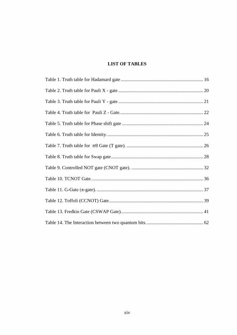
LIST OF TABLES

Table 1. Truth table for Hadamard gate ..................................................................... 16

Table 2. Truth table for Pauli X - gate ....................................................................... 20

Table 3. Truth table for Pauli Y - gate ....................................................................... 21

Table 4. Truth table for Pauli Z - Gate. ..................................................................... 22

Table 5. Truth table for Phase shift gate .................................................................... 24

Table 6. Truth table for Identity. ................................................................................ 25

Table 7. Truth table for 𝜋8 Gate (T gate). ................................................................ 26

Table 8. Truth table for Swap gate ............................................................................. 28

Table 9. Controlled NOT gate (CNOT gate). ............................................................ 32

Table 10. TCNOT Gate. ............................................................................................. 36

Table 11. G-Gate (π-gate). ......................................................................................... 37

Table 12. Toffoli (CCNOT) Gate............................................................................... 39

Table 13. Fredkin Gate (CSWAP Gate). .................................................................... 41

Table 14. The Interaction between two quantum bits. ............................................... 62

xv

LIST OF FIGURES

Figure 1. Satisfying the Moor's Law for progressing the technology of computers. ... 3

Figure 3. An arbitrary block diagram of a three-qubits quantum circuit. Where the

index i = 8, since the circuit has three inputs. ............................................................ 11

Figure 4. Hadamard gate ............................................................................................ 16

Figure 5. Bloch sphere represented a) the evaluated |1⟩ state, b) the evaluated |0⟩

state. ........................................................................................................................... 17

Figure 6. Pauli x - gate .............................................................................................. 18

Figure 7. NOT gate participates to construct, a) CNOT gate ; b) Toffoli gate. ........ 18

Figure 8. The Bar Chart (3 dimensions), represents the probability of evaluation of

single-qubit bases states due to NOT Gate operation. ............................................... 19

Figure 9. Pauli Y - gate. ............................................................................................. 20

Figure 10. Pauli Z - Gate ............................................................................................ 21

Figure 11. The Bar Chart (3 dimensions), represents the probability of evaluation of

single-qubit bases states due to Pauli-Z Gate operation. ........................................... 22

Figure 12. Phase Shift Gate. ....................................................................................... 23

Figure 13. The Identity gate operator. ........................................................................ 24

Figure 14. The Bar Chart (3 dimensions), represents the 2x2 identity matrix

operation. .................................................................................................................... 25

Figure 15. 𝜋8 Gate (T gate). ..................................................................................... 25

Figure 16. Swap gate .................................................................................................. 26

xvi

Figure 17. The Bar Chart (3 dimensions), represents the probability of evaluation of

two-qubit bases states due to SWAP Gate operation. ................................................ 28

Figure 18. Controlled NOT gate (CNOT gate) .......................................................... 29

Figure 19. The Bar Chart (3 dimensions), represents the probability of evaluation of

two-qubit bases states due to CNOT Gate operation. ................................................ 31

Figure 20. TCNOT Gate. .......................................................................................... 33

Figure 21. The Bar Chart (3 dimensions), represents the probability of evaluation of

two-qubit bases states due to TCNOT Gate operation. .............................................. 35

Figure 22. Toffoli (CCNOT) Gate. ............................................................................ 38

Figure 23. The Bar Chart (3 dimensions), represents the probability of evaluation of

three-qubit bases states due to Toffoli Gate operation. .............................................. 39

Figure 24. Fredkin Gate (CSWAP Gate) ................................................................... 40

Figure 25. The Bar Chart (three dimensions), represents the probability of evaluation

of three-qubit bases states, due to Fredkin Gate operation. ....................................... 41

Figure 26. a) Hydrogen atom in |0⟩ state, b) The state |1⟩, c) Superposition of states

12(|0⟩+ |1⟩). ............................................................................................................ 44

Figure 27. Level scheme for 40

Ca containing only the states. ................................... 45

Figure 28. Static magnetic field (𝐵0) along "z" axis and alternative time dependent

magnetic field (𝐵1) with angular frequency 𝜔 along "y" axis................................... 48

Figure 29. A schematic of the Polarization of single photon mode. (A) Horizontal

Polarization, (B) Vertically Polarization, (c) Left Circular Polarization, (d) Right

Circular Polarization, ................................................................................................. 51

Figure 30. RCP and LCP respectively. ...................................................................... 51

Figure 31. An elementary quantum logic gate using optical QED, ........................... 52

xvii

Figure 32. The physical system in the static form (the probability amplitude of each

state does not change during the time) ....................................................................... 57

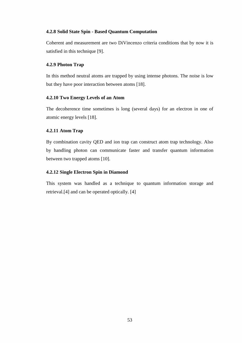
Figure 33. The physical system in the dynamical form (flipping of bases states and

superposition of states with probability amplitudes 15 𝑎𝑛𝑑 25 ) .............................. 59

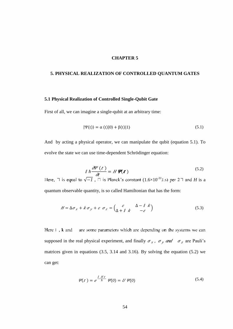
Figure 34. The overall single quantum system, which is simulated quantum

computer, the first, third and second parts demonstrate input, output (that is time-

independent without change of the state) and operation (flipping the state from 0 to 1

and vice versa)............................................................................................................ 59

Figure 35. The physical system in the dynamical (flipping of bases states and

superposition of states) and statically(the gate does not change states and work as an

Identity matrix) form.(Bar Chart representation) ....................................................... 60

Figure 36. The Bar Chart in three dimensions, that shows the physical realization of

CNOT gate, by using Ising interaction. ..................................................................... 63

Figure 37. The CNOT Gate Operation, either |00⟩ state nor |01⟩ do not change their

state, and remain constant; The other bases states (|10⟩ state and |11⟩ state) flipped to

each other. .................................................................................................................. 64

xviii

LIST OF SYMBOL/ABBREVIATION

ABBRE. FULL TEXT

CNOT Controlled NOT

NMR Nuclear Magnetic Resonance

C-Phase gate Conditional-Phase Gate

𝜎𝑥 ,𝑦 ,𝑧 Single-Qubit Pauli Operator

QED Quantum Electrodynamics

QC Quantum Computing

Reduced Planck’s Constant

CPU Central Processing Unit

VLSI Very Long Scale Integration

xix

PERSONAL INFORMATION

Name and Surname: Ibrahim Nazem Qader AL-Jaf

Nationality: Iraqi

Birth place and date: Al-Sulaymaniyah / 01.01.1987

Mariel status: Married

Phone number: Iraq Mob.: +964 750 4933789

Turkey Mob.: ---------

Fax: ------

Email:i.nazm@yahoo.com, ibrahimnazemqader@gmail.com, i.nazm@hotmail.com

EDUCATION

Degree Graduate school Year

Master Gaziantep University 2011-2013

Bachelor Salahaddin University 2008-2009

High School Sadogi /Piranshahr / Iran 2003-2004

WORK EXPERIENCE

Time Place Enrollment

2009-Present Salahaddin University / ERBIL Physical assistant

PUBLICATIONS

N. Q. Ibrahim, and R. KOÇ ―Simulation of Controlled physical quantum Gates by

using Mathematica‖ International Journal of Computer Science and Network

Security (IJCSNS), under review.

xx

LANGUAGES

Kurdish (Native)

Persian (Native)

English (Good)

Arabic (Medium)

Turkish (weak)

HOBBIES

Reading

Studying

Conferences and Seminars

Religions

1

CHAPTER 1

1. INTRODUCTION

The information technology has been changing the cover of human society.

Computer devices and their usage are in the center of these progresses. Efforts to

scheme and build devices to help humans in their computing tasks is started from

ancient times. The first mechanical computers were built from rather than 2000 years

beforehand, and generation of the modern electronic computers started in the last

century. They have many forms, some of them just performing a unique function (i.e.

Automobiles and home appliances), and some of them are very advanced (like

supercomputers for the design of airplanes and the simulation of climate changes)

[22].

In 1623, the addition and subtraction operations were performed by a calculating

clock was constructed by Professor Wilhelm Schickard. Some years later in 1666

Samuel Morland who was a British construct a mechanical device to accomplishing

basic arithmetic calculation as addition and subtraction, but the multiplying

operation in 1777 was satisfied.

In 1854, a famous paper was titled "An Investigation of the Laws of Thought"

published by George Boole that introduced the basic logic of binary ("true" &

"false"). By using this idea Alan Turing in 1936, wrote the concept of the universal

computing machine. And finally in 1939, John V. Atanasoff who was a professor at

Iowa State College, by using Boolean algebra designed an electronic computer that

could accomplish arithmetic calculation.

2

The artificial of electronic computers, during progressing of science, spatially

theoretical of modern physics and practicalities of factories, have several short

generations.

1.1 Generation of Computers

1.1.1 First Generation (1940-1956) Vacuum Tubes:

In fact, when someone looking for the history of computers, can see, during the

second world war a first electronic computer was constructed by British engineers by

helping the famous mathematician, Alan M. Turing. It could decode the message of

the Germans were encoded by ENIGMA machine.

1.1.2 Second Generation (1955-1965) Transistors:

The John Bardeen and Walter Brattain were two inventors that in 1947 at Bell

Laboratory made the first transistor, it was one of the important inventions in

humanity.

1.1.3 Third Generation (1964-1971) Integrated Circuit:

After invention integrated circuit (IC) in 1959, the computer's memory and processor

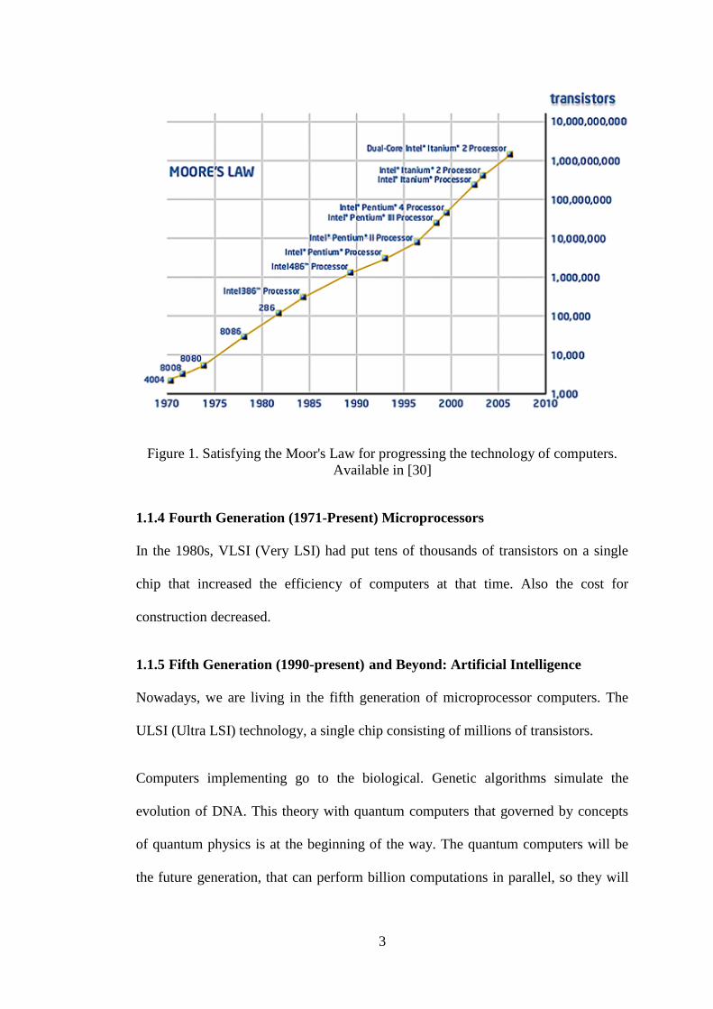
become smaller. Moor has predicted that the number of transistors which occupied

the specific area in an integrated circuit doubles every 18 months approximately

[18,21]( On the other hand empirical results in the last years shows that the power of

quantum computers duplicate every six years [32]).

3

Figure 1. Satisfying the Moor's Law for progressing the technology of computers.

Available in [30]

1.1.4 Fourth Generation (1971-Present) Microprocessors

In the 1980s, VLSI (Very LSI) had put tens of thousands of transistors on a single

chip that increased the efficiency of computers at that time. Also the cost for

construction decreased.

1.1.5 Fifth Generation (1990-present) and Beyond: Artificial Intelligence

Nowadays, we are living in the fifth generation of microprocessor computers. The

ULSI (Ultra LSI) technology, a single chip consisting of millions of transistors.

Computers implementing go to the biological. Genetic algorithms simulate the

evolution of DNA. This theory with quantum computers that governed by concepts

of quantum physics is at the beginning of the way. The quantum computers will be

the future generation, that can perform billion computations in parallel, so they will

4

make a big revolution in science and spatially in humankind, and will change the

cover of the world in general.

The quantum mechanical systems can be represented by matrices. For a single

particle system, it is not so difficult to controlling its parameters to manipulate the

system, but when the numbers of particles in a system increased, the matrix's

parameters manually uncontrollable. Since, the computers have handled to progress

themselves, and to design the future computer generation, in fact, we must use, by

now, the classical computers to simulate each part of hardware (i.e. Physical

structure) and software (i.e. Programming of computer for various tasks).

1.2 Scope of the Thesis

In this thesis we will see the progress of the quantum computation, theoretically and

experimentally, also, the new techniques to realize quantum gates. The structure of

the thesis is as follows:

1.3 Outline of the Thesis

Chapter 2, contains a general scope of quantum computation and the name of some

centers are working in this area. Also several importance of the field that makes it

become an interlining field for many scientists in the world. In the continuation of

the chapter there are some mathematical tools which we need in the quantum

computation. Finally in brief, we will talk about quantum computer, which is the

objective of all researchers in the scope.

Chapter 3 contains the definition and the matrix representation of single, two and

three qubit quantum gates in several ways. We have tried to demonstrate how one

can decompose a quantum gate or even a circuit to the bases computational states,

5

and by using rules of linear algebra (i.e. Kronecker product and scalar product) can

get a single square matrix for whole of quantum circuit. Also we can see the

simulation of quantum gates as (bar chart) in three dimensions by using the

"Wolfram Mathematica" program.

Chapter four includes the literature survey of realization of various physical systems,

which were performed experimentally, by using some groups of researcher. These

realizations are in the scope of satisfying David DiVincenzo criteria, entangled

multi-qubits for a desired time during operational process. More details are taken for

some systems with high fidelity to construct the large scale quantum computer.

Chapter five, is the most important part of this dissertation, that contains illustration

of some quantum gates by solving the time-dependent Schrödinger equation for

several desired Hamiltonians and by controlling the parameters of time-dependent

probability equation, we have tried to show the physical realization of quantum gates

theoretically. In addition, the simulations of the systems and graphs are performed by

using "Wolfram Mathematica" program.

Chapter six is covering the discussion of the results and conclusions of the study with

the future work.

6

CHAPTER 2

2. QUANTUM COMPUTATION

2.1 Introduction

The quantum computation (or nano computation [18]) and quantum information are

based on some postulates of quantum mechanics [10,20]. But nowadays, they are not

just a branch of physics but many mathematician, chemist and computer scientists

attempt whether experimentally or in theory. [17] This area is trying to study for

developing computer technology and based on quantum’s principles. [33]

The goal of quantum computing is to find new definition for defined instruments

(transistors, bit, gate...etc) by using new techniques to harnessing quantum effects in

the nano scale material. To getting this aim one has to know about quantum

mechanics and information science. [18]

Current centers of research in quantum computing include D-Wave, [18] , DARPA

(Defense Advanced Research Projects Agency) with the U.S. military [26],

Clarendon Laboratory at Oxford or the Centre for Quantum Computing at

Cambridge, both in the UK, [35], MIT [27], IBM [28], Oxford University[29], and

the Los Alamos National Laboratory [31].

2.2 Combination of Quantum Computer

The quantum computer is combined of three parts: [2]

1. The input of information as encoded qubits.

7

2. A quantum process unit consisting of quantum gates to accomplish unitary

transformations on input data.

3. The last part is a measurement on the output state and breakdown the

superposition of states to the computational basis of the individual qubits.

The block diagram of a general form of a quantum computer is as follows:

Figure 2. A block diagram of an quantum computer, which consisting of three parts:

input information, quantum unit processor (QUP) and the last part is a measurable

states of quantum information.

2.3 Important of Quantum Computation

Every bit physically represented by a capacitor or a point is magnetized on disc. So

the main differences between classical and quantum computers appear from this

point that all classical bit represented by the quantities that controlled by laws of

classical physics but quantum bits or quantum gates governed by quantum mechanics

features [17]. Some of these quantum mechanical properties are as following:

1. Superposition

2. Entanglement

3. Phase

8

4. Reversibility

5. No-Cloning

6. Quantum Error Correction (QEC)

7. Quantum teleportation

2.4 The Mathematical Concepts that Represented of Quantum Gates in term of

Dirac Notation and Hubbard Operators:

We can represent every quantum gates by using either Dirac notations or Hubbard

operators 𝑋𝑟𝑐 , (where X is represented a unit matrix element and each r and c are the

rows and column number respectively).

Hubbard operators obey the following rule:

𝑋𝑟𝑐𝑋𝑚𝑛 = 𝑋𝑟𝑛𝛿𝑐𝑚 (2.1)

𝑤𝑕𝑒𝑟𝑒 𝛿𝑐𝑚 = 0 𝑖𝑓 𝑐 ≠ 𝑚1 𝑖𝑓 𝑐 = 𝑚

For example:

𝑋11𝑋22 = 1 00 0

0 00 1

= 0

𝑋12𝑋21 = 0 10 0

0 01 0

= 1 00 0

= 𝑋11

The matrix representation of NOT gate (Pauli-X or Sigma-1 gate) can be construct

by the following ways:

𝑁𝑂𝑇 = 𝑋12𝑋22 + 𝑋22𝑋21 = 0 10 0

0 00 1

+ 0 00 1

0 01 0

= 0 10 0

+ 0 01 0

= 0 11 0

(2.2)

9

Also we can write it in another form:

𝑁𝑂𝑇 = 𝑋11𝑋12 + 𝑋21𝑋11 = 1 00 0

0 10 0

+ 0 01 0

1 00 0

= 0 10 0

+ 0 01 0

= 0 11 0

(2.3)

In the other side, Dirac notations can be used. The notation, bra | is represented

row vector and ket or (state vector) was symbolized in the form | ⟩ is the column

vector. Also by taking conjugate of ket we get bra [10]. Therefore, the symbol

is so - called bra-ket [5].

A vector in space 𝕔 𝑛 and vector in complex space 𝕔 𝑛∗ are denoted respectively

by[12,17] :

| 𝑥⟩ =

𝑥1𝑥2..𝑥𝑛

, 𝑦 | = {𝑦1 ,𝑦2 … ,𝑦𝑛} (2.4)

𝑤𝑕𝑒𝑟𝑒 𝑥𝑛 ,𝑦𝑛 ∈ 𝕔

Dirac notations similarly can be used to construct quantum gates from basic unit

matrices:

𝑋𝑟𝑐 = | 𝑟 − 1⟩ 𝑐 − 1 | (2.5)

The above equation is an outer product (kronecker product). Also the inner product

of a two orthogonal vector, is satisfy:

10

𝑛 𝑚 = 𝛿𝑛𝑚 (2.6)

𝑤𝑕𝑒𝑟𝑒 𝛿𝑛𝑚 = 1 𝑤𝑕𝑒𝑛 𝑛 = 𝑚0 𝑤𝑕𝑒𝑛 𝑛 ≠ 𝑚

For instance the result of multiplication of a square matrix 𝑋𝑟𝑛 and | 𝑚⟩ or two

square matrices 𝑋𝑟𝑛𝑋𝑚𝑠 become:

𝑟⟩ 𝑛 𝑚⟩ = | 𝑟⟩𝛿𝑛𝑚 (2.7)

𝑟⟩ 𝑛 𝑚 𝑠 = | 𝑟⟩ 𝑠|𝛿𝑛𝑚 (2.8)

Now by using these rules we can construct NOT gate that is consisting two parts, one

of them can converts |0⟩ to |1⟩ and the other part has conversion |1⟩ to |0⟩ duty. as

following:

0⟩ 1 = 0 01 0

(2.9)

1⟩ 0 = 0 10 0

(2.10)

by adding the equations (2.9) and (2.10), we get NOT gate:

0⟩ 1 + 1⟩ 0 = 0 01 0

+ 0 10 0

= 0 11 0

(2.11)

Since, one of quantum computational conditions for a matrix to being useable as a

quantum gate is unitary properties. To check if a square matrix is a unitary or not we

can use the following way:

𝐴𝐴∗ = 𝑛⟩ 𝑚 + 𝑚⟩ 𝑛 𝑛⟩ 𝑚 + 𝑚⟩ 𝑛

= |𝑛⟩ 𝑚|𝑛⟩ 𝑚| + |𝑛⟩ 𝑚|𝑚⟩ 𝑛| + |𝑚⟩ 𝑛|𝑛⟩ 𝑚| + |𝑚⟩ 𝑛|𝑚⟩ 𝑛|

= |𝑛⟩ 𝑛| + |𝑚⟩ 𝑚| = 𝐼 (2.12)

11

(Where 𝑛 ≠ 𝑚 , 𝐼 is identity matrix and 𝐴∗ is adjoin of A).

By these ways we can mathematically construct unitary matrices to manipulate

qubits and controlled quantum gates.

2.5 Quantum Circuit

Quantum circuit is an array of quantum gates, that their arrangement for different

tasks changed. The quantum information inter a quantum circuit and after evaluation

get out as an output. In a quantum circuit each component represented by a square

matrix, which is produced by kronecker product. In the quantum circuit conveniently

the inputs are in the left side of the circuit and the outputs are in the other side.

Figure 3. An arbitrary block diagram of a three-qubits quantum circuit. Where the

index i = 8, since the circuit has three inputs.

Therefore, from the left side the matrices are start from 𝑍𝑖 to 𝐴𝑖 (in the matrix 𝐴𝑖 , i

represented the dimension of the matrix), then the final result is a single square

matrix which its dimension is equal to i :

12

𝑀𝑖 = 𝐴𝑖𝐵𝑖 … .𝑌𝑖 𝑍𝑖 (2.13)

For example we have two matrices A and B with dimension two:

𝐴2 = 𝑎1,1 𝑎1,2

𝑎2,1 𝑎2,2 ,𝐵2 =

𝑏1,1 𝑏1,2

𝑏2,1 𝑏2,2 (2.14)

The matrix multiplication of A and B of the equation (2.14) is as follows:

𝐶3,3 = 𝑐1,1 𝑐1,2

𝑐2,1 𝑐2,2 (2.15)

where:

𝑐1,1 = 𝑎1,1𝑏1,1 + 𝑎2,1𝑏2,1 ; 𝑐1,2 = 𝑎1,1𝑏1,2 + 𝑎1,2𝑏2,2;

𝑐2,1 = 𝑎2,1𝑏1,1 + 𝑎2,2𝑏2,1 ; 𝑐2,2 = 𝑎2,1𝑏1,2 + 𝑎2,2𝑏2,2 ;

2.6 Quantum Computer

Constructing quantum computer is the end of quantum computational field. The first

idea was formed when scientists thought about limitation of classical computing and

the obstacle that laws of physics makes when the size of computers according to

moor’s law have daily squeezing. [18]

The beginning to this field back to early of the seventies that suggested by an

unlucky researcher (Stefan Wiesner) who worked on the last year of the seventies but

his work was published in 1983. Furthermore, Charles Bennett in IBM, Paul Benioff

of Argonne National Laboratory [18], David Deutsch in Oxford university and

finally Richard feynman in California Institute of Technology separately worked on

this category. [17]

13

It is a quantum mechanical Turing machine [14] to accomplishing quantum

information processing [3] without dissipate energy [14]. There is an abstract model

of such computer was suggested and is so-called ―Quantum Turing Machine‖ or

―Universal Quantum Computer‖ [18] Schrodinger equation is a way to simulate

quantum computer [2]. for one qubit ,the Schrodinger equation can be used.

Quantum computer is not a hyper computer but it is faster than traditional computer

[25]. Nowadays it is one of active field because of its potential power [13] that is one

of particular feature with respect to its classical partner. By getting its realization we

may use of its potential power to encrypted messages, factoring a large number or

used for internet business [13].

Photons have poor interaction with each other but they are the best candidate to

transfer information from one point to another point. In contrast, the particles such

atoms, ions and electrons have faster interaction but have slower movement. Atoms

can change their energy levels so fast which is an advantage of them for quantum

computers [18]. So by harnessing atomic scale particles, designer will generate new

efficiency memory and processor in the future computer.

Read, write and information processing are three properties of every computers [18].

Quantum computers similar to classical computers consist of two parts, one of them

is software which includes quantum algorithms e.g. Shor’s algorithm. The other part

is hardware that needs to realize quantum logic gates and quantum memory register

(qubit) physically [8,10]. Consequently we can summarized them; classical computer

consists of LOAD–RUN–READ and quantum computer has PREPARE–EVOLVE–

MEASURE parts [10].

14

One may ask how one can write in quantum computer ? One method is excited atoms

by using laser beam. For instance the atom of hydrogen, when we want write 0, we

don’t need to do anything, but to writing 1 by using proper laser pulse atom exited

from ground state to an exited state. In contrast, if the atom be in an exited state, the

laser pulse makes the atom back to ground state (zero state) [18].

A quantum computer with 30 qubits has power of a traditional computer with its

processor could accomplish 10 Tera computation per second (10 Teraflops) on

decimal number. By now, the faster super computer has 2 Teraflops [18]. They are

going to evolve in the future, simulations of global warming and weather prevision

would be much more accurate. Medical, Social and Physical sciences would gain a

very strong instrumentation in having novel levels of resolution in data for research

[35].

In a few years later the quantum computers will produced in the laboratories by

physicists, chemists, computer scientists and mathematicians [18]. By now, Bruce

Kane who is a Australian physicist has designed a quantum computer in which based

on nuclear spins of phosphorus silicon atoms [10]. Also, In 2011 ―D-Wave Systems‖

company, was claimed that successfully make a quantum computer with 128 qubit

processor. They made superconductor circuits with Niobium (Nb) in a very low

temperature [18].

15

CHAPTER 3

3. QUANTUM GATES AND THEIR USAGE

3.1 Introduction

In quantum computation we execute unitary operations on arrange of qubits. These

operations are called gates. When we want to construct a quantum computer we are

meant at manufacture the qubits, the elements saving information using physical

properties, and another important part to manipulate information. That is, finding a

good way to store information and read it out would not be enough - we would like

to run it by gates. So, for each type of qubit accomplishment, we would like to build

a reasonable procedure of accomplishing operations on it [27].

Quantum gates are operators that evaluate a quantum system from one state to

another. Every quantum mechanical operators are linear. According to quantum

mechanical principle the operators which can be used in quantum computation are

unitary and represented as a matrix that apply to an arbitrary quantum state (qubit)

[17]. Also a quantum circuit is composed of single quantum gates and CNOT gate

[11].

There are many ways to represented the elements of quantum computer (i.e.

Quantum gates, qubits). Also, one can use the Mathematica packages, like:

QDENSITY [62,54], to simulate quantum computer's part.

16

3.2 Quantum Gate Manipulates on Single Qubit

3.2.1 Hadamard Gate

Figure 4. Hadamard gate

Hadamard gate [3,6,8,10,17] can simulate non-deterministic computation. It is a

single-qubit gate that can construct some composed states from basis states is as

(equation 3.1):

H |0⟩ = 1

2 (|0⟩ + |1⟩) , H|1⟩ =

1

2 (|0⟩ - |1⟩) (3.1)

Hadamard gate is able to make an entanglement between two qubits [3]. In general

we can write [6]:

H | x⟩ = 1

2 (−1)𝑥𝑧𝑧 ∈{ 0,1} |z⟩ (3.2)

Also by measuring the output of this quantum gate yields 50 percentage |0⟩ or |1⟩

computational basis states. The truth table is as below:

Table 1. Truth table for Hadamard gate

Input Output

0 𝟏

𝟐 (|0⟩ + |1⟩)

1 𝟏

𝟐 (|0⟩ - |1⟩)

17

In the figure (5) we can see the state of qubit after Hadamard operator act on it.

(a) (b)

Figure 5. Bloch sphere represented a) the evaluated |1⟩ state, b) the evaluated |0⟩ state.

The Hadamard gate can be described by the following operator [6,8,10,17]:

H = 1

2 (|0⟩ 1|+|0⟩ 1|+|1⟩ 0|-|1⟩ 1|)

= 1

2

10 ⊗ 1 0 +

10 ⊗ 0 1 +

01 ⊗ 1 0 −

01 ⊗ 0 1

= 1

2

1 00 0

+ 0 10 0

+ 0 01 0

+ 0 00 −1

= 1

2

1 11 −1

(3.3)

Also there is another way to get the same result, by using two matrices of Pauli:

𝐻 =1

2(𝜎𝑥 + 𝜎𝑧) (3.4)

Here we mention some properties of Hadamard gate [26]:

𝐻2 = 1 , 𝐻 𝜎𝑥 𝐻 = 𝜎𝑧 , 𝐻 ≡ 𝐻𝑒𝑟𝑚𝑖𝑡𝑖𝑎𝑛 𝑚𝑎𝑡𝑟𝑖𝑥 (3.5)

18

3.2.2 NOT Gate

Pauli X - Gate (NOT gate) [1,3,6,10] is another reversible single-qubit operator that

is the most important quantum gate. Graphically it is represented by:

Figure 6. Pauli x - gate

It participates to construct other quantum gates like Controlled-NOT (CNOT) [61]

gate which is a two-qubit quantum gate and Control-Control-NOT (Toffoli) gate

which is a three-qubit operator:

(a) (b)

Figure 7. NOT gate participates to construct, a) CNOT gate ; b) Toffoli gate.

19

The gate which is represented as the first Pauli matrix, can be obtained from bellow

operator:

𝜎𝑥= |0⟩ 1| + |1⟩ 0| = 0 10 0

+ 0 01 0

= 10 ⊗ 0 1 +

01 ⊗ 1 0

= 0 11 0

(3.6)

The result of a circuit of gates (Hadamard ⤑ Z gate ⤑ Hadamard) is a NOT gate:

When it applies to a superposition state, during its action, the probability amplitude is

flipping 𝛼 0⟩+ 𝛽 1⟩ 𝑡𝑜 𝛽 0⟩+ 𝛼|1⟩ or in the form of matrix we have:

𝜎𝑥 𝛼𝛽 =

𝛽𝛼 𝑎𝑛𝑑 𝑣𝑖𝑠𝑒 𝑣𝑒𝑟𝑠𝑎 𝜎𝑥

𝛽𝛼 =

𝛼𝛽 (3.7)

Figure 8. The Bar Chart (3 dimensions), represents the probability of evaluation of

single-qubit bases states due to NOT Gate operation.

.

Now, we give an example with basis states |0⟩ and |1⟩, now by acting 𝜎𝑥 to each of

them we get [17]:

20

𝜎𝑥 |0⟩ = 0 11 0

. 10 =

01 = |1⟩ (3.8)

𝜎𝑥 |1⟩ = 0 11 0

. 01 =

10 = |0⟩ (3.9)

There are some properties of NOT gate as following [26]:

0 𝜎𝑥 0⟩ = 0

1 𝜎𝑥 1⟩ = 0

𝜎𝑥 .𝜎𝑥 = 𝐼

𝜎𝑥 ≡ 𝐻𝑒𝑟𝑚𝑖𝑡𝑖𝑎𝑛 𝑚𝑎𝑡𝑟𝑖𝑥

(3.10)

(3.11)

(3.12)

(3.13)

Consequently, the truth table for single-quantum NOT gate is given in table (2):

Table 2. Truth table for Pauli X - gate

Input Output

𝜶 𝟎⟩+ 𝜷|𝟏⟩ 𝜷|𝟎⟩+ 𝜶|𝟎⟩ 0 𝟏

1 𝟎

3.2.3 Pauli Y-Gate

Pauli Y-Gate [6] is another Pauli matrix operator, which is graphically represented

by the figure (9):

Figure 9. Pauli Y - gate.

Also, its matrix can obtain from the operator:

21

𝜎𝑦 = 1⟩ 0 − 0⟩ 1 𝑒𝑖 𝜋2 =

10 ⊗ 0 −𝑖 +

01 ⊗ 𝑖 0

= 0 −𝑖0 0

+ 0 0𝑖 0

= 0 −𝑖𝑖 0

(3.14)

When it applies to a superposition state, during its action, the probability amplitude is

flipping 𝛼 0⟩+ 𝛽 1⟩ 𝑡𝑜 𝛽 0⟩+ 𝑖 𝛼|1⟩ or in the form of matrix we have:

𝜎𝑦 𝛼𝛽 =

−𝑖𝛽𝑖 𝛼

𝑎𝑛𝑑 𝑣𝑖𝑠𝑒 𝑣𝑒𝑟𝑠𝑎 𝜎𝑦 𝛽𝛼 =

−𝑖𝛼𝑖 𝛽

(3.15)

Finally we can show the truth table in the table (3):

Table 3. Truth table for Pauli Y - gate

Input Output

𝜶 𝟎⟩+ 𝜷|𝟏⟩ −𝒊 𝜷|𝟎⟩+ 𝒊|𝜶⟩

|0⟩ 𝒊 |𝟎⟩

|1⟩ −𝒊|𝟏⟩

3.2.4 Pauli Z -Gate

The third and the final Pauli matrix is Z - Gate [3,6,10], that its scheme is graphically

it represented by the figure(10):

Figure 10. Pauli Z - Gate

And one can get the Z - Gate matrix by using following operator that consist of bases

states (|0⟩ and |1⟩) [6,10]:

22

𝜎𝑧 = 0⟩ 0 − 1⟩ 1 = 10 ⊗ 1 0 −

01 ⊗ 0 1 =

1 00 0

− 0 00 1

= 1 00 −1

(3.16)

The action on a single-qubit in superposition is:

𝜎𝑧(𝛼|0⟩+ 𝛽|1⟩) = (𝛼 0⟩ − 𝛽|1⟩) (3.17)

Figure 11. The Bar Chart (3 dimensions), represents the probability of evaluation of

single-qubit bases states due to Pauli-Z Gate operation.

The truth table that consist of all possible inputs and outputs is shown in the table

(4):

Table 4. Truth table for Pauli Z - Gate.

Input Output

𝜶|𝟎⟩+ 𝜷|𝟏⟩ 𝜶 𝟎⟩ − 𝜷|𝟏⟩

0 𝟎

1 −𝟏

3.2.5 Phase Shift Gate

The graphic symbol for Phase Shift Gate [6,8] was come which it has a shape with a

line and square that a label "S" on it:

23

Figure 12. Phase Shift Gate.

The general form of phase shift gate is as bellow matrix:[8]

𝑆 = 1

2

1 00 𝑒𝑖𝜃

(3.18)

The action on bases states (|0⟩ and|1⟩) only changes |1⟩ state by a phase of (ⅇiθ) as

we can see:

0⟩ → 0⟩ & |1⟩ → ⅇiθ|1⟩ (3.19)

And its action on a single qubit in superposition becomes:

𝛼 0⟩+ 𝛽|1⟩ → 𝛼 0⟩+ 𝛽𝑒𝑖𝜃 |1⟩ (3.20)

The realization has been done by using Quantum electrodynamics (QED) experiment

[10].

𝑆 = 1

2

1 00 𝑖

(3.21)

As we can see it is one of spatial form of the phase shift operator, and it is obtained

when (θ=π/2 ,5π/2, 9π/2 ...etc).

Here is the truth table for every input and output convenient quantum information in

the single-qubit form:

24

Table 5. Truth table for Phase shift gate

Input Output

𝜶|𝟎⟩+ 𝜷|𝟏⟩ 𝜶 𝟎⟩+ 𝜷 𝒆𝒊𝜽 |𝟏⟩

0 𝟏

𝟐|𝟎⟩

1 𝟏

𝟐e−iθ|𝟏⟩

3.2.6 Identity Operator

Graphically it represented in the figure (13):

Figure 13. The Identity gate operator.

The operator for a (2x2) Identity matrix is represented in the equation (3.22):

𝜎0 = 𝐼 = |0⟩ 0| + |1⟩ 1| = 10 ⊗ 1 0 +

01 ⊗ 0 1 =

1 00 0

+ 0 00 1

= 1 00 1

(3.22)

When it applies to a superposition state, during its action, the state of qubit, remains

constant.

25

Figure 14. The Bar Chart (3 dimensions), represents the 2x2 identity matrix

operation.

The truth table for (2x2) identity operator with one input and one output has given as

the table (6):

Table 6. Truth table for Identity.

Input Output

𝜶|𝟎⟩+ 𝜷|𝟏⟩ 𝜶|𝟎⟩+ 𝜷|𝟏⟩

0 𝟎

1 𝟏

3.2.7 T- Gate

Graphical scheme of T - Gate ( 𝜋

8 Gate ) [3,6] is represented by the figure (15):

Figure 15. 𝜋

8 Gate (T gate).

26

Now, by using quantum computational basis states (|0⟩ and |1⟩) we can construct the

matrix representation of the gate:

𝑇 = |0⟩ 0| + 𝑒𝑖𝜋4 |1⟩ 1| =

1 0

0 eiπ4 (3.23)

Square of T gate is equal to phase gate (T = S ). [3]

The truth table that shows us the action of operator on input states to getting new

state as a output, is come in the table (7):

Table 7. Truth table for 𝜋

8 Gate (T gate).

Input Output

𝜶|𝟎⟩+ 𝜷|𝟏⟩ 𝛼 0⟩+ 𝛽𝑒𝑖𝜋4 |1⟩

|0⟩ |0⟩

|1⟩ 𝑒𝑖𝜋4 |1⟩

3.3 Quantum Gate Manipulates on Two Qubits:

3.3.1 Swap Gate

Figure 16. Swap gate

Also, the graphical symbol of swap gate is as shown:

27

And its matrix representation is [8]:

𝑈𝐴𝑊𝐴𝑃 =

1 00 0

0 01 0

0 10 0

0 00 1

(3.24)

We can prove the equation (3.24) as the following:

𝑈𝐴𝑊𝐴𝑃 = 00⟩ 00 + 01⟩ 10 + 10⟩ 01 + 11⟩ 11

= 0⟩ 0 ⊗ 0⟩ 0 + 0⟩ 1 ⊗ 1⟩ 0 + 1⟩ 0 ⊗ 0⟩ 1 + 1⟩ 1 ⊗ 1⟩ 1

=

1 00 0

0 01 0

0 10 0

0 00 1

(3.25)

When it applies to a two-qubit with similar basis state (|11⟩ or |00⟩) do not change,

otherwise the gate as an operator swap 0 with 1. [8] It is shown as follows:

|00⟩ → |00⟩, |01⟩ → |10⟩, |10⟩ → |01⟩, |11⟩ → |11⟩

And for a two-qubit in superposition we have:

𝛼 00⟩+ 𝛽 01⟩+ 𝛾 10⟩+ 𝛿 11⟩ → 𝛼 00⟩+ 𝛾 01⟩+ 𝛽 10⟩ + 𝛿 11⟩

Or any entangled states:

SWAP ( 𝛾|01⟩+ 𝜉|10⟩ ) = SWAP

0𝛾𝜉0

=

0𝜉𝛾0

= 𝜉|01⟩+ 𝛾|10⟩ (3.26)

28

SWAP ( 𝛾|00⟩+ 𝜉|11⟩ ) = SWAP

𝛾00𝜉

=

𝛾00𝜉

= 𝛾|00⟩+ 𝜉|11⟩ (3.27)

Figure 17. The Bar Chart (3 dimensions), represents the probability of evaluation of

two-qubit bases states due to SWAP Gate operation.

Therefore, the truth table contains the inputs and outputs, that each qubit effected on

the other partner and swap it is in the table (8):

Table 8. Truth table for Swap gate

Input Output

Q1 Q2 Q1 Q2

|0⟩ |0⟩ |0⟩ |0⟩

|0⟩ |1⟩ |1⟩ |0⟩

|1⟩ |0⟩ |0⟩ |1⟩

|1⟩ |1⟩ |1⟩ |1⟩

3.3.2 Controlled NOT Gate (CNOT gate)

C-NOT gate [8,21,27] is one of universal quantum gates [10,23]. Barenco showed (in

1995) that any multiple qubit quantum logic gate 𝑈(2𝑁) consisting on universal

CNOT gate [14]. It is similar to the NAND classical gate. Graphically its represented

by the figure (18):

29

Figure 18. Controlled NOT gate (CNOT gate)

Every n-qubit operations can be constructed by a combination of this gate [21]. As

an example we can mention the Beam splitter based structure, that can be worked as

a quantum CNOT gate [20].

Here we give two methods for obtaining the matrix operator of CNOT gate, by using

Wolfram Mathematica and manually:

a) Its matrix representation is can be obtained by the following operator

[8,17,20,23,24]:

𝑈𝐶𝑁𝑂𝑇 = 00⟩ 00 + 01⟩ 01 + 10⟩ 11 + 11⟩ 10 =

1 00 1

0 00 0

0 00 0

0 11 0

(3.28)

b) C-Not gate can be constructed from particular CPhase gate [3]

(Hadamard gate → two qubit gate → Hadamard gate) [23]

𝐶𝑁𝑂𝑇 = 𝐻 2 . 𝑐𝑈11 .𝐻 2 = 𝐼 ⊗ 𝐻 . 𝐼 ⊕ 𝑍 . 𝐼 ⊗ 𝐻

30

The position of the target and Controlled qubits of CNOT can be exchanged with

each other when we conjugate it with H on both qubits:

3.3.2.1 Unitary Specialty

One of conditions for an operator be one of universal quantum gate is, unitary

specialty. So, we want to check whether CNOT matrix is unitary matrix or not:

𝐶𝑁𝑂𝑇.𝐶𝑁𝑂𝑇 =

1 00 1

0 00 0

0 00 0

0 11 0

.

1 00 1

0 00 0

0 00 0

0 11 0

=

1 00 1

0 00 0

0 00 0

1 00 1

= 𝐼𝑑𝑒𝑛𝑡𝑖𝑡𝑦 𝑀𝑎𝑡𝑟𝑖𝑥 ⇒ 𝑈𝑛𝑖𝑡𝑎𝑟𝑦 𝑀𝑎𝑡𝑟𝑖𝑥 (3.29)

Now, by acting on basis states, we can see that the second qubit result is conform to

the result of a classical XOR gate [8,20,23]:

00⟩ → 00⟩ , |01⟩ → 01⟩, |10⟩ → 11⟩, |11⟩ → |10⟩

The general form of its action is coming as following: [25]

𝐶𝑁𝑂𝑇 𝑎, 𝑏⟩ = 𝑎,𝑎 ⊗ 𝑏⟩ (3.30)

𝑤𝑕𝑒𝑟𝑒 𝑎, 𝑏 ∈ {0,1}

Detail : it swaps |10⟩ with |11⟩ and vice versa [10]. In another word, the first input

can act on the second and flip it if its value be 1 [17,21].

31

Proof:

Let me show by giving an example to show, when the first qubits be in 0 states, the

second one after acting CNOT gate do not change:

For instance we have two qubits |𝜳⟩ and |∅⟩ in superposition and also they are flip

of each other:

𝛹⟩ = 𝜉 1⟩+ 𝛾 |0⟩ = 𝜉 01 + 𝛾

10 =

𝛾𝜉 & ∅ ⟩ = 𝛾 1⟩+ 𝜉 |0⟩

= 𝛾 01 + 𝜉

10 =

𝜉𝛾 (3.31)

Figure 19. The Bar Chart (3 dimensions), represents the probability of evaluation of

two-qubit bases states due to CNOT Gate operation.

Suppose, for a two-qubit CNOT gate, the state |0⟩ as the first qubit and the state |𝛹⟩

in the second one (|0,𝛹⟩):

|0⟩ ⊗ 𝛹⟩ = 0⟩ ⊗ 𝜉 1⟩+ 𝛾 0⟩ = 𝜉 0,1⟩+ 𝛾 0,0⟩

= 𝜉

0100

+ 𝛾

1000

=

0𝜉00

+

𝛾000

=

𝛾𝜉00

(3.32)

32

Then by applying CNOT gate, we get:

𝐶𝑁𝑂𝑇 |0,𝛹⟩ = 𝐶𝑁𝑂𝑇

𝛾𝜉00

=

𝛾𝜉00

= |0,𝛹⟩ (3.33)

As we can see the state |0,𝛹⟩ stay constant without any change. The truth table for

this universal quantum gate is as follows:

Table 9. Controlled NOT gate (CNOT gate).

Input Output

Control Target Control Target

0 0 0 0

0 1 0 1

1 0 1 1

1 1 1 0

3.3.2.2 Bell States Construction

We can construct the entangled Bell states:

1

2(|00⟩+ |11⟩),

1

2(|01⟩+ |10⟩),

1

2( 01⟩ − |10⟩) 𝑎𝑛𝑑

1

2( 00⟩ − |11⟩) (3.34)

by using a Hadamard gate located at the first qubit state and the CNOT gate in the

next of it:

33

3.3.3 TCNOT Gate

TCNOT Gate [7] is another unitary quantum gate that graphically is shown in the

figure (20), the location of control and target exchanged together (target is located in

the first and controlled quantum gate in the second):

Figure 20. TCNOT Gate.

The structure consistence is equal with the CNOT gate but, since the component

element has a different position, so its action be different.

𝑇𝐶𝑁𝑂𝑇 =

1 00 0

0 00 1

0 00 1

1 00 0

(3.35)

One can find the matrix representation of TCNOT gate, by following mathematical

ways:

1- The first one is as follows:

𝑈𝐶𝑁𝑂𝑇 = 00⟩ 00 + 01⟩ 11 + 10⟩ 10 + 11⟩ 01 =

1 00 0

0 00 1

0 00 1

1 00 0

(3.36)

2) TCNOT gate similar to the CNOT gate can be constructed from particular CPhase

gate:

34

(Hadamard gate → two_qubit gate → Hadamard gate)

𝐶𝑁𝑂𝑇 = 𝐻 1 . 𝑐𝑈11 .𝐻 1 = 𝐻⊗ 𝐼 . 𝐼 ⊕ 𝑍 .𝐻⊗ 𝐼

=1

2

1 11 −1

⊗ 1 00 1

. 1 00 1

⊕ 1 00 −1

.1

2

1 11 −1

⊗ 1 00 1

=1

2

1 00 1

1 00 −1

1 00 −1

−1 00 −1

.

1 00 1

0 00 0

0 00 0

1 00 −1

.1

2

1 00 1

1 00 −1

1 00 −1

−1 00 −1

=

1 00 0

0 00 1

0 00 1

1 00 0

(3.37)

The position of target and Controlled qubits of TCNOT also can be exchanged with

each other when we conjugate it with H on both qubits:

In general, the action, similar to CNOT gate, make a change in target quantum gate

output and the second qubit, controlled quantum gate, without change. But, because

35

of differences in position of the components, the outputs will be different from

CNOT gate:

𝑇𝐶𝑁𝑂𝑇|𝑎, 𝑏⟩ = |𝑎 ⊗ 𝑏, 𝑏⟩ ,𝑤𝑕 𝑒𝑟𝑒 𝑎, 𝑏 ∈ {0,1}

(3.38)

𝑇𝐶𝑁𝑂𝑇|00⟩ =

1 00 0

0 00 1

0 00 1

1 00 0

.

1000

=

1000

= |00⟩ (3.39)

𝑇𝐶𝑁𝑂𝑇|01⟩ =

1 00 0

0 00 1

0 00 1

1 00 0

.

0100

=

0001

= |11⟩ (3.40)

𝑇𝐶𝑁𝑂𝑇|10⟩ =

1 00 0

0 00 1

0 00 1

1 00 0

.

0010

=

0010

= |10⟩ (3.41)

𝑇𝐶𝑁𝑂𝑇|11⟩ =

1 00 0

0 00 1

0 00 1

1 00 0

.

0001

=

0100

= |01⟩ (3.42)

From the results, we can get that the quantum gate flips first qubit when the second

one is in the |1⟩ state.

Figure 21. The Bar Chart (3 dimensions), represents the probability of evaluation of

two-qubit bases states due to TCNOT Gate operation.

Like other quantum gate, TCNOT gate to be useful in quantum computation must

pass the unitary condition:

36

𝑇𝐶𝑁𝑂𝑇.𝑇𝐶𝑁𝑂𝑇 =

1 00 0

0 00 1

0 00 1

1 00 0

.

1 00 0

0 00 1

0 00 1

1 00 0

=

1 00 1

0 00 0

0 00 0

1 00 1

= 𝐼𝑑𝑒𝑛𝑡𝑖𝑡𝑦 𝑀𝑎𝑡𝑟𝑖𝑥 ⇒ 𝑈𝑛𝑖𝑡𝑎𝑟𝑦 𝑚𝑎𝑡𝑟𝑖𝑥 (3.43)

The truth table for this universal quantum gate is shown in the table (10):

Table 10. TCNOT Gate.

Input Output

Target Control Target Control

0 0 0 0

0 1 1 1

1 0 1 0

1 1 0 1

3.3.3.1 Bell States created by TCNOT Gate

In similar to the CNOT gate we can use TCNOT gate and Hadamard gate together to

create Bell states. Here is the circuit's shape which its component location is shown

and the mathematical method:

3.3.4 G-Gate

G-Gate [23] is another two-qubit quantum state that its matrix representation is

shown as following:

37

𝐺 = 00⟩ 00 + 01⟩ 01 + 10⟩ 10 + 𝑒𝑖𝜃 ( 11⟩ 11

= 0⟩ 0 ⊗ 0⟩ 0 + 0⟩ 0 ⊗ 1⟩ 1 + 1⟩ 1 ⊗ 0⟩ 0 + 𝑒𝑖𝜃 1⟩ 1 ⊗ 1⟩ 1

=

1 00 1

0 00 0

0 00 0

1 00 𝑒𝑖𝜃

(3.44)

Also the name of gate is changed to (π gate). By taking the value (±𝜋) instead of θ.

When this quantum gate acts on every two qubit quantum bases state, leaves the state

without change, just |11⟩ is changed to 𝑒𝑖𝜃 |11⟩:

|00⟩ → |00⟩, |01⟩ → |01⟩, |10⟩ → |10⟩, |11⟩ → 𝑒𝑖𝜃 |11⟩

In general its action on basis states:

00⟩ → 𝑒𝑖𝜑00 00⟩ , 01⟩ → 𝑒𝑖𝜑01 01⟩, 10⟩ → 𝑒𝑖𝜑10 10⟩, |00⟩ → 𝑒𝑖𝜑11 |11⟩

where: 𝜑00 ,𝜑01 ,𝜑10 = 0 & 𝜑11 = ±𝜋

Finally, the truth table of G-gate is taken as the table (11):

Table 11. G-Gate (π-gate).

Input Output

|0⟩ |0⟩ |0⟩ |0⟩

|0⟩ |1⟩ |0⟩ |1⟩

|1⟩ |0⟩ |1⟩ |0⟩

|1⟩ |1⟩ |1⟩ |1⟩

3.4 Quantum Gate Manipulates on Three Qubits

3.4.1 Toffoli (CCNOT) Gate

It has three input and three output, two of them are controlled qubit without any

manipulating on input state and the other is target which is flipped by the other qubits

38

if both of them are set of |1⟩ and if one or both of them are |0⟩ is left alone [5,11].

Graphically it is represented by figure(22):

Figure 22. Toffoli (CCNOT) Gate.

The matrix representation can produced by the following operator [8]:

𝑇𝑜𝑓𝑓𝑜𝑙𝑖 = 000⟩ 000 + 001⟩ 001 + 010⟩ 010 + 011⟩ 011 + 100⟩ 100

+ 101⟩ 101 + 110⟩ 111 + 111⟩ 110

= 0⟩ 0 ⊗ 0⟩ 0 ⊗ 0⟩ 0 + 0⟩ 0 ⊗ 0⟩ 0 ⊗ 1⟩ 1 + 0⟩ 0 ⊗ 1⟩ 1

⊗ 0⟩ 0 + 0⟩ 0 ⊗ 1⟩ 1 ⊗ 1⟩ 1 + 1⟩ 1 ⊗ 0⟩ 0 ⊗ 0⟩ 0 + 1⟩ 1

⊗ 1⟩ 1 ⊗ 0⟩ 0 + 1⟩ 1 ⊗ 1⟩ 1 ⊗ 0⟩ 1 + 1⟩ 1 ⊗ 1⟩ 1

⊗ 1⟩ 0

=

1 0 00 1 0

0 00 0

0 0 00 0 0

0 0 10 0 0

0 01 0

0 0 00 0 0

0 0 00 0 00 0 00 0 0

0 10 00 00 0

0 0 01 0 00 0 10 1 0

(3.45)

39

The CCNOT (Toffoli) gate manipulates the third qubit in a three input qubit state,

when the first two qubits are in 1 state, at that time the operator flip the third one, as

you can see in the below:

000⟩ → 000⟩, 001⟩ → 001⟩, 010⟩ → 010⟩, 011⟩ → 011⟩,

|100⟩ → |100⟩, |101⟩ → |101⟩, |110⟩ → |111⟩, |111⟩ → |110⟩

Detail: it swaps |110⟩ with |111⟩ and vice versa.

Figure 23. The Bar Chart (3 dimensions), represents the probability of evaluation of

three-qubit bases states due to Toffoli Gate operation.

The Truth table for Controlled-Controlled-NOT gate is as the table (12):

Table 12. Toffoli (CCNOT) Gate.

Input Output

0 0 0 0 0 0

0 0 1 0 0 1

0 1 0 0 1 0

0 1 1 0 1 1

1 0 0 1 0 0

1 0 1 1 0 1

1 1 0 1 1 1

1 1 1 1 1 0

40

3.4.2 Fredkin Gate (CSWAP Gate)

Figure 24. Fredkin Gate (CSWAP Gate)

The final quantum gate that here is investigated, is the Fredkin quantum gate, which

has three inputs and three outputs. Its matrix representation is [8]:

𝐹𝑟𝑒𝑑𝑘𝑖𝑛 = 000⟩ 000 + 001⟩ 001 + 010⟩ 010 + 011⟩ 011

+ 100⟩ 100 + 101⟩ 110 + 110⟩ 101 + 111⟩ 111

= 0⟩ 0 ⊗ 0⟩ 0 ⊗ 0⟩ 0 + 0⟩ 0 ⊗ 0⟩ 0 ⊗ 1⟩ 1 + 0⟩ 0

⊗ 1⟩ 1 ⊗ 0⟩ 0 + 0⟩ 0 ⊗ 1⟩ 1 ⊗ 1⟩ 1 + 1⟩ 1

⊗ 0⟩ 0 ⊗ 0⟩ 0 + 1⟩ 1 ⊗ 1⟩ 1 ⊗ 1⟩ 0 + 1⟩ 1

⊗ 1⟩ 0 ⊗ 0⟩ 1 + 1⟩ 1 ⊗ 1⟩ 1 ⊗ 1⟩ 1

=

1 0 00 1 0

0 00 0

0 0 00 0 0

0 0 10 0 0

0 01 0

0 0 00 0 0

0 0 00 0 00 0 00 0 0

0 10 00 00 0

0 0 00 1 01 0 00 0 1

(3.46)

41

Detail: Its action on qubits becomes swapping |101⟩ with |110⟩ and vice versa:

000⟩ → 000⟩, 001⟩ → 001⟩, 010⟩ → 010⟩, 011⟩ → 011⟩,

|100⟩ → |100⟩, |101⟩ → |110⟩, |110⟩ → |101⟩, |111⟩ → |111⟩

Figure 25. The Bar Chart (three dimensions), represents the probability of evaluation

of three-qubit bases states, due to Fredkin Gate operation.

The truth table for Fredkin quantum gate is as the table (13):

Table 13. Fredkin Gate (CSWAP Gate).

Input Output

0 0 0 0 0 0

0 0 1 0 0 1

0 1 0 0 1 0

0 1 1 0 1 1

1 0 0 1 0 0

1 0 1 1 1 0

1 1 0 1 0 1

1 1 1 1 1 1

42

CHAPTER 4

4. REALIZATION AND ACHIEVEMENTS OF QUBITS AND QUANTUM

GATES

4.1 Introduction

We know that constructing quantum computer’s building block (qubits and logic gates)

by several techniques and different size and features are studied other experimentally or

during abstract mathematical modeling.

Therefore, to the realization of any physical system we can use experimental result and

mathematical modeling of systems. There are many experiments were performed by

scientists and Hamiltonian models to investigate input, accomplish process and finally

the output. As an example Quantum hybrid device [37,38] consists of three most

important parts: memory (natural atom), quantum processor unit (artificial atoms and

molecule)[40] and flying qubits (photon) [45-47] to transfer information. The natural

atoms consisting of ions and neutral atoms that long decoherence time, is one of

advantageous feature of them to be used in quantum memory, and similarly, we have

artificial atoms like semiconductor quantum dots [41-44], electron or nuclear spin in

solid and superconducting circuits [48,49] which have a so faster operation than other

candidates and become a best nomination to construct quantum processor [9].

In most of the instrumentation that was suggested to realize any part of quantum

computer [39,50], they have used cooling systems as a technique for initialization by

43

reducing the kinetic energy of moving during temperature T, for instance, in two

energy level systems , as an electron in Hydrogen atom [51], the electron will be in

minimum energy level (ground state) with a high accuracy. In the other hand, cooling

down some systems such as liquid state NMR, obviously known that the state of the

system will change [14].

The most practical realization was achieved in this field is the teleportation of

quantum information was performed in 1997 at Institute of Experimental Physics,

University of Innsbruck in Austria [17].

Decoherence time [52,53] is the biggest problem with realization quantum gates in

all quantum systems [23] that we will observe when continuing afterwards.

4.2 Realization of Various Physical Systems

4.2.1 Trapped Ion

Nowadays, quantum computational researchers focused on building a large-scale

ion-trap quantum computer [3,4,8,10,18]. The technique was proposed by Peter

Zoller and Ignacio Cirac in 1995 [3,8,10]. and they handled ―Paul‖ trap [8]. They

succeeded to verification 90% implemented CNOT gate operation by using

beryllium ion as encoding qubits [10]. Also the efforts of Wolfgang Paul who was a

researcher lead to introduce the concept of ion trap experiment and share to

progressing atomic spectroscopy [8].

Naturally the ions with a similar charge push away each other, and they are

squeezing by the electric fields of the trap.

44

Quantum information is stored to electronic energy levels. The experimentalist use

cold trapped ions as a technique so the information able to stored in ground state

levels [8].

Ions in a linear trap are confined by a harmonic oscillator in three directions {x, y,

z}[55-57] and in this case the frequency of x direction is less than the others. The

linear electromagnetic trap was used in this technique [8].

To decrease the noise we can use ultra-high vacuum which makes improving of the

ion trap system from the collision of unwanted particles [8].

Both nuclear and valence electron spin determine the state of the qubit (figure 26). If

both of them have the same spin, they represent |1⟩ qubit state and otherwise qubit

be in |0⟩ state. While the spin of nuclear and valence electron have both up and

down simultaneously we say it is in superposition [8].

Figure 26. a) Hydrogen atom in |0⟩ state, b) The state |1⟩ , c) Superposition of states 1

2(|0⟩+ |1⟩).

Available at [8]

Prof. Christopher Monroe said "a cadmium atom can stay in its state for a thousand

years" [8,15,18].

45

e.g. we use a laser to pumping in a low temperature .We supposed to (𝐶𝑎 +) ion

(𝐷5/2) level represents state |1⟩ and 𝑆 3/2 as state |0⟩ .

Figure 27. Level scheme for 40

Ca containing only the states.

Available at [16]

4.2.1.1 Ion Trap Satisfies Fifth David DiVincenzo Criteria:

1. Scalability : in several ions can make superposition between ground state |0⟩

and exited state |1⟩ .

2. Initialization state : by using a laser with a proper frequency and power can

manipulate state of qubits.

3. Decoherence time : the decoherence time is 1000 degrees greater than gate

operations.

4. A universal set of quantum gates.

5. Capable to measure each qubit because for instance in 𝐂𝐚 + ion (figure 27)

as an example the difference energy level of 𝐏 𝟏 /𝟐 and 𝐃𝟓 /𝟐 (∆𝑬𝟏 ) is

contrary from 𝐏 𝟏 /𝟐 and 𝐒 𝟏 /𝟐 (∆𝑬𝟐 ). So when the ion in the ground state

46

𝐒 𝟏 /𝟐 absorbs a convenient photon exited to 𝐏 𝟏 /𝟐 and by emitted a photon

goes back to the ground state and we can measure the fluorescent light of

|0⟩ state more accurately. [8,57,59,60]

4.2.1.2 (Instrumentation) The Spectroscopy Device in Ion Trap Experiment

a) A sample,

b) A glass tube to hold the sample and should be designed as an evacuated

chamber,

c) Superconducting magnet,

d) A source of radiofrequency resonator that must have desired phase, power,

and frequency .

e) The cooling system, so-called optical molasses [8,10]

4.2.1.3 Some Experimental Results of Trapped Ion

a) Long decoherence time has been shown by several experiments, [3,8]

b) It is possible to work at room temperature, [8]

c) Poor scalability,[8]

d) Slow gate operation, [8]

e) Initialization of states is difficult, [8]

f) The most qubit used in ion trap is 14 entangled ions was recorded by the

Innsbruck group [32] in March 2011, [8]

g) Eight calcium ions were used in quantum computers, [3]

h) DJ Algorithm has employed [4,10] with a 𝐂𝐚 + by Innsbruck group at

2003, [8]

47

i) By using an ion trap technique the 3- entanglement particle was created [10].

and Greenberger–Horne–Zeilinger (GHZ) and W, was succeeded to realize

more than 14 qubits [9].

j) In 1995 the C-NOT quantum logic gate with a single cold trapped 𝐵𝑒 + ion

experiment was performed by NIST group [6,8].

k) Quantum error correction and decoherence free qubits was demonstrated [9].

4.2.1.4 Negative Effects that are Affected in Ion Traps

a) Temperature; [8]

b) Collision between ions makes the loss of quantum information;

c) Since the ions are charged particles, their interaction with the environment is

greater than neutral atoms [18].

4.2.1.5 Various Shapes of Ion Trap

a) The cylindrically symmetric 3D ring trap; [8]

b) The linear trap with a combination of cavity QED;

c) The symmetric quadrupole linear trap.

4.2.2 Nuclear Spins

This system was handled as a technique to quantum information storage and retrieval

[4] and can be manipulated by hyperfine coupling [4]. Also NMR technology can be

used as a method to manipulate spin in nuclei of atoms [10].

The spin direction ordered due to the effects of a desired NMR. At the time, all

nuclear oriented to minimum energy level, therefore they aligned direction similar to

the applying field then convenient radio frequency can be handled to manipulate

them [10].

48

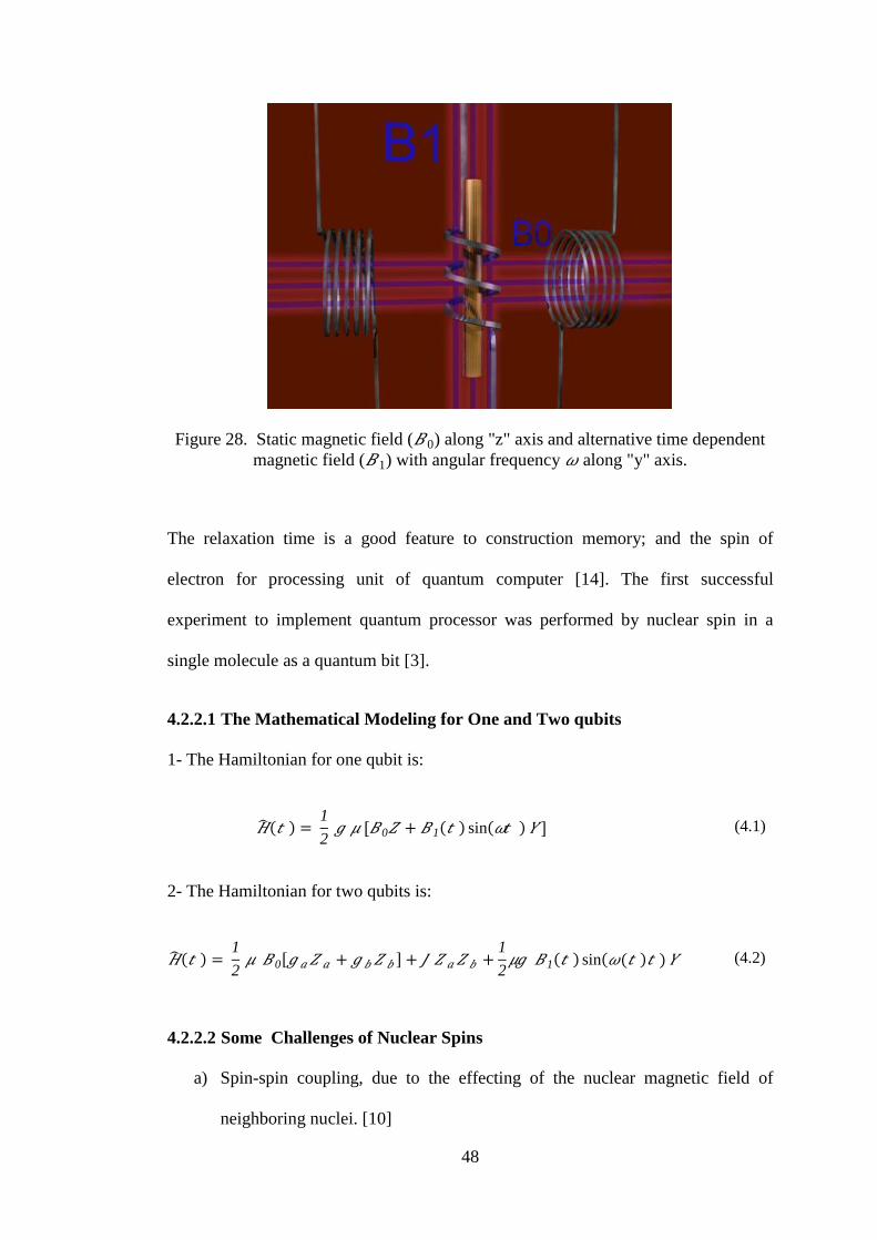
Figure 28. Static magnetic field (𝐵 0) along "z" axis and alternative time dependent

magnetic field (𝐵 1) with angular frequency 𝜔 along "y" axis.

The relaxation time is a good feature to construction memory; and the spin of

electron for processing unit of quantum computer [14]. The first successful

experiment to implement quantum processor was performed by nuclear spin in a

single molecule as a quantum bit [3].

4.2.2.1 The Mathematical Modeling for One and Two qubits

1- The Hamiltonian for one qubit is:

𝐻 𝑡 = 1

2 𝑔 𝜇 [𝐵 0𝑍 + 𝐵 1 𝑡 sin 𝜔𝑡 𝑌 ] (4.1)

2- The Hamiltonian for two qubits is:

𝐻 𝑡 = 1

2 𝜇 𝐵 0 𝑔 𝑎 𝑍 𝑎 + 𝑔 𝑏 𝑍 𝑏 + 𝐽 𝑍 𝑎 𝑍 𝑏 +

1

2𝜇𝑔 𝐵 1 𝑡 sin 𝜔(𝑡 𝑡 )𝑌 (4.2)

4.2.2.2 Some Challenges of Nuclear Spins

a) Spin-spin coupling, due to the effecting of the nuclear magnetic field of

neighboring nuclei. [10]

49

b) Chemical shift, due to nearest electron orbits of neighboring atoms [10].

4.2.3 Quantum Dots

Quantum dots [4,8,10,14,18] are made from semiconductor crystals and their

capability to save the electron charge for a long time has made them to be one of the

best candidates for constructing memory of computers [18].

They are similar to tiny island of semiconductor which are taken on an electronic

chip [18] and electrically isolated. The electrical voltage is used to manipulate the

amount of free electron inside quantum dots. Also by applying a laser beam with

proper frequency to changing the state of qubit from |0⟩ to |1⟩ [10].

This technique has several disadvantages (short coherence time) and advantage (like

easy to scalability) [10]. Nowadays, quantum dot working on low temperature [18].

The technology gets to a level that can produce quantum dots (artificial atom) and

coupled quantum dots (artificial molecule). And because of their particular electrical

feature is the reason that one can manipulate all parameters of them by using external

voltage. [14] By using electric field one can confine an electron in a semiconductor

quantum dot.

4.2.4 Nuclear Magnetic Resonance (NMR)

Its abundance applications and tremendous parallelism make this technique be

preference with respect to others [3,4,8,10]. The spin of the nucleus is used as a

quantum bit in NMR technique [8]. This physical system consists of two parts. The

first part is a sample like: 1H,

13C,

19F,

19N and ...etc. That their protons should have

spin 1

2 . The other part is the NMR spectroscopy device [8]. Also the electromagnetic

50

waves uses for NMR technology is radio frequency that can retouch state of spin of

nuclear [8].

There are some other applications of NMR (magnetic resonance image (MRI) in

medicine and chemistry and as a qubits [3,8].

4.2.4.1 Experimental Result in NMR

a) Satisfy two qubit algorithms and seven qubits for factoring number 15, that

demonstrated Shor’s algorithm experimentally [3].

b) DJ Algorithm has employed experimentally [4].

c) Long coherence time [3].

4.2.5 Superconducting Qubit

One of advantage of this technique is used huge number (millions or billions) of

electrons so it is not necessary to control each individual electron alone. Nowadays,

superconductors can produce in low temperature (mK), so this is one of

disadvantages of them [18]. In the other hand they occupy small area (about μm), so

can concentrate on chips [9] and can be control its electrical by standard microwave

and radio - frequency (RF) [3].

The energy relaxation times from nanoseconds progressed to microseconds (μs) [9]

after 10 years ago [3] and three qubits were successfully entangled in this technique.

[9]

4.2.6 Polarization of a Photon

Photons work as flying qubit [6,8,10,18] but they have a poor desire to interact with

each other so it makes difficult to build more than one qubit gate.

51

Figure 29. A schematic of the Polarization of single photon mode. (A) Horizontal

Polarization, (B) Vertically Polarization, (c) Left Circular Polarization, (d) Right

Circular Polarization,

Available at[20].

Figure 30. RCP and LCP respectively.

Available at[34]

4.2.6.1 The Instrumentation of a Polarization Photon

a) Photon generator

b) Photo-detector

c) Phase shifter,

d) A beam splitter.

52

4.2.7 Cavity Quantum Electrodynamics (QED)

This theory investigates the interaction of individual atoms with optical field [8]. The

polarization of photons represented qubits is sent by optical resonator and after

manipulating by trapping atoms inside the cavity, get out as a result of computing

[8].

It can demonstrate single quantum phase gate [19] but constructing a quantum circuit

is a challenge to extend this technology [10].

As an experimental result we can mention multi qubit was performed [23].

4.2.7.1 Instrumentation of (QED)

a) Trapped atom as a sample like Calcium (Ca), Cesium(Cs), Rubidium(Rb) and

Barium(Ba);

b) A cavity;

c) Optical resonator.

Figure 31. An elementary quantum logic gate using optical QED,

Available at [8]

53

4.2.8 Solid State Spin - Based Quantum Computation

Coherent and measurement are two DiVincenzo criteria conditions that by now it is

satisfied in this technique [9].

4.2.9 Photon Trap

In this method neutral atoms are trapped by using intense photons. The noise is low

but they have poor interaction between atoms [18].

4.2.10 Two Energy Levels of an Atom

The decoherence time sometimes is long (several days) for an electron in one of

atomic energy levels [18].

4.2.11 Atom Trap

By combination cavity QED and ion trap can construct atom trap technology. Also

by handling photon can communicate faster and transfer quantum information

between two trapped atoms [10].

4.2.12 Single Electron Spin in Diamond

This system was handled as a technique to quantum information storage and

retrieval.[4] and can be operated optically. [4]

54

CHAPTER 5

5. PHYSICAL REALIZATION OF CONTROLLED QUANTUM GATES

5.1 Physical Realization of Controlled Single-Qubit Gate

First of all, we can imagine a single-qubit at an arbitrary time:

Ψ t ⟩ = ⍺ t 0⟩+ β t |1⟩ (5.1)

And by acting a physical operator, we can manipulate the qubit (equation 5.1). To

evolve the state we can use time-dependent Schrödinger equation:

𝕚 ħ𝜕𝛹 (𝑡 )

𝜕𝑡= 𝐻 𝜳(𝒕 )

(5.2)

−1 (1.6×10-31

H is a

quantum observable quantity, is so called Hamiltonian that has the form:

𝐻 = ∆𝜎 𝑥 + 𝑘 𝜎 𝑦 + 휀 𝜎 𝑧 = 휀 ∆ − 𝕚 𝑘

∆+ 𝕚 𝑘 −휀 (5.3)

supposed in the real physical experiment, and finally 𝜎 𝑥 , 𝜎 𝑦 𝑎𝑛𝑑 𝜎 𝑧 are Pauli’s

matrices given in equations (3.5, 3.14 and 3.16). By solving the equation (5.2) we

can get:

𝛹 𝑡 = 𝑒𝕚 𝐻 𝑡

ħ 𝛹 0 = 𝑈 𝛹(0) (5.4)

55

𝑈 = 𝑒𝕚 𝐻 𝑡

ħ (5.5)

Ψ 0 = α 0 + β 0 = α 0

β 0 =

𝑎 + 𝕚 𝑏𝑐 + 𝕚 𝑑

(5.6)

Here, U is a unitary transformation, that can transform the state Ψ 0 , from an initial

time (t=0) to any arbitrary time (t).

By now, we can use "Wolfram Mathematica" as a powerful program to simulate the

single qubit system, and investigate it as a general. By taking the equation (5.3) in

the Schrödinger equation (5.2), we can get a solution in the matrix form:

𝑈 = Cos[𝑡𝜔 ]−

ⅈ휀 Sin[𝑡𝜔 ]

𝜔ℏ−

(𝑘 + ⅈ𝛥 )Sin[𝑡𝜔 ]

𝜔ℏ(𝑘 − ⅈ𝛥 )Sin[𝑡𝜔 ]

𝜔ℏCos[𝑡𝜔 ] +

ⅈ휀 Sin[𝑡𝜔 ]

𝜔ℏ

The above matrix is a 2x2 unitary matrix, that by giving different values to the

parameters, one can get, any known single-qubit quantum gates. For instance the

matrix U act on a single - qubit in a superposition of two states that has the form:

ϒ 0⟩+ 𝜉 |1⟩

0⟩𝑎𝑛𝑑 |1⟩ and respectively.

Since, after evaluation, we will have the form:

⍺ 0⟩+ 𝛽 |1⟩

That each values 𝛼 𝑎𝑛𝑑 𝛽 are the probability amplitude for new evaluated state.

56

𝛼 = −(𝑘 + ⅈ𝛥 )𝜉 Sin[𝑡𝜔 ]

𝜔ℏ+ 𝛾 Cos 𝑡𝜔 −

ⅈ 휀 Sin 𝑡𝜔

𝜔ℏ (5.7)

𝛽 =𝛾 𝑘 − ⅈ𝛥 Sin 𝑡𝜔

𝜔ℏ+ 𝜉 Cos 𝑡𝜔 +

ⅈ 휀 Sin 𝑡𝜔

𝜔ℏ (5.8)

By having the probability amplitudes (𝛼 𝑎𝑛𝑑 𝛽 ) we can leave the initial qubit

without change during processing, and the operator, operate as an identity matrix;

Also we can construct an arbitrary 2x2 unitary matrices that can change the state of

qubit during the evaluation.

5.1.1 Single Qubit Memory

First of all, we make a 2x2 matrix (or "PauliMatrix[0]" [36]) to simulate single-qubit

memory (storage part of quantum computer) by following considerations:

휀 ≫ 𝑘 ,∆

휀 = 25 ∗ 106; 𝑘 = 0; 𝛥 = 0; 𝑡 = 10

−9; ℏ =1

2Pi; 𝜔 = 2Pi 𝛥 2 + 𝑘 2 + 𝜖 2;

The real value of Planck's constant is ( 6.626068 × 10-34

m2 kg / s) [15], but we take

the value 1 to make our computation easy; Also the units of the quantities are

omitted.

Since, the probability amplitude 𝛾 after evaluation transform to 𝛼 and 𝜉 to 𝛽 . So,

the initial probability amplitudes in principle must not change and remain constant.

When the values of 𝛾 𝑎𝑛𝑑 𝜉 are chosen 0 and 1 and vice versa, so the value of 𝛼

and 𝛽 must be 0 and 1 respectively (𝛾 = 𝛼 , 𝜉 = 𝛽 ) as we can see in the figure

(32):

57

Figure 32. The physical system in the static form (the probability amplitude of each

state does not change during the time)

Therefore , by using given values to the parameters, we can check that the state

satisfy one of principles of quantum mechanics, that says: "the normalization of a

state should equal to one". Since, the summation of probability functions must equal

to 1:

|𝛼 |2 + |𝛽 |2 = 1 (5.9)

58

5.1.2 Single Qubit Processor

By now, to give a dynamical rule to the quantum system to become a processor , the

NOT gate as an example, (σx or its Wolfram Mathematica code is: PauliMatrix [1]).

We can give new values to the parameters in the equations (5.7 and 5.8), as

following:

(ε ≪ k ,∆)

ℏ =1

2π;𝜔 = 2Pi 𝛥 2 + 𝑘 2 + 𝜖 2; 휀 = 0; 𝑘 = 0; 𝑡 = 10

−9;

By using the given values in the equation (5.9), one can find the exact value of :

(∆= 2.5 × 108 𝑜𝑟 ∆= −2.5 × 10

8)

The following figures (33, 34 and 35), are the results of the single-qubit simulation

by using the Mathematica program, in each freezing state of the qubit and dynamical

form in term of bases states and superposition of bases states.

59

Figure 33. The physical system in the dynamical form (flipping of bases states and

superposition of states with probability amplitudes 1

5 𝑎𝑛𝑑

2

5 )

Figure 34. The overall single quantum system, which is simulated quantum

computer, the first, third and second parts demonstrate input, output (that is time-

independent without change of the state) and operation (flipping the state from 0⟩ to 1⟩ and vice versa).

60

Figure 35. The physical system in the dynamical (flipping of bases states and

superposition of states) and statically(the gate does not change states and work as an

Identity matrix) form.(Bar Chart representation)

5.2 Physical Realization of Controlled Two-Qubit Gate

The state of two-qubit quantum gate controlled by the solution of time evaluation

Schrodinger equation:

∅ 𝑡 ⟩ = 𝑒−𝑖 𝐻 𝑡

ħ ∅ 0 ⟩ = 𝑈 |∅ (0)⟩ (5.10)

61

Each of the states of ∅ 𝑡 ⟩𝑎𝑛𝑑 |∅ (0)⟩ are represented by a 4x1 matrices which

are called column matrices because they have four rows and one column. Therefore,

the operator (𝑈 = 𝑒−𝑖 𝐻 𝑡

ħ ) is a square 4x4 matrix.

5.2.1 General Hamiltonian for Two-Quantum bits

In general, for a system that has an anisotropic interaction the Hamiltonian is

represented by:

𝐻 = 𝐻𝑎 +𝐻𝑏 + 𝐻𝑖 (5.11)

In the equation (5.11), 𝐻𝑎 ,𝐻𝑏 𝑎𝑛𝑑 𝐻𝑖 are the Hamiltonian for first qubit, second

qubit and energy interaction between them respectively. And each of them in general

can be represented as following:

𝐻𝑎 = ∆𝑎 𝜎 𝑥𝑎 + 𝑘 𝑎 𝜎 𝑦𝑎 + 휀 𝑎 𝜎 𝑧𝑎 (5.12)

𝐻𝑏 = ∆𝑏 𝜎 𝑥𝑏 + 𝑘 𝑎 𝜎 𝑦𝑏 + 휀 𝑏 𝜎 𝑧𝑏 (5.13)

𝐻𝑖 = 𝐽 𝑥 𝜎 𝑥𝑎 𝜎 𝑥𝑏 + 𝐽 𝑦 𝜎 𝑦𝑎 𝜎 𝑦𝑏 + 𝐽 𝑧 𝜎 𝑧𝑎 𝜎 𝑧𝑏 (5.14)

In the equations (5.12, 5.13 and 5.14), ∆𝑎 ,∆𝑏 ,𝑘 𝑎 ,𝑘 𝑏 , 휀 𝑎 𝑎𝑛𝑑 휀 𝑏 are the

parameters of both qubits (a and b), also 𝐽 𝑥 , 𝐽 𝑦 𝑎𝑛𝑑 𝐽 𝑧 are coupling constants.

So the Hamiltonian of the system become:

𝐻 = ∆𝑎 𝜎 𝑥𝑎 + 𝑘 𝑎 𝜎 𝑦𝑎 + 휀 𝑎 𝜎 𝑧𝑎 + ∆𝑏 𝜎 𝑥𝑏 + 𝑘 𝑎 𝜎 𝑦𝑏 + 휀 𝑏 𝜎 𝑧𝑏

+ 𝐽 𝑥 𝜎 𝑥𝑎 𝜎 𝑥𝑏 + 𝐽 𝑦 𝜎 𝑦𝑎 𝜎 𝑦𝑏 + 𝐽 𝑧 𝜎 𝑧𝑎 𝜎 𝑧𝑏 (5.15)

There are, 𝜎 𝑥𝑎 ,𝜎 𝑦𝑎 𝑎𝑛𝑑 𝜎 𝑧𝑎 the tensor products of Pauli matrices with 2 × 2

Identity matrix and 𝜎 𝑥𝑏 , 𝜎 𝑦𝑏 and 𝜎 𝑧𝑏 are the tensor product of 2 × 2 Identity

matrix with each x, y and z, Pauli matrices, respectively. By taking the result of each

of the above outer products in Hamiltonian equation, we can get:

62

𝐻

=

휀 𝑎 + 휀 𝑏 + 𝐽 𝑧 ∆𝑏 − 𝑖 𝑘 𝑏∆𝑏 + 𝑖 𝑘 𝑏 휀 𝑎 − 휀 𝑏 − 𝐽 𝑧

∆𝑎 − 𝑖 𝑘 𝑎 𝐽 𝑥 − 𝐽 𝑦 𝐽 𝑥 + 𝐽 𝑦 ∆𝑎 − 𝑖 𝑘 𝑎

∆𝑎 + 𝑖 𝑘 𝑎 𝐽 𝑥 + 𝐽 𝑦 𝐽 𝑥 − 𝐽 𝑦 ∆𝑎 + 𝑖 𝑘 𝑎

−휀 𝑎 + 휀 𝑏 − 𝐽 𝑧 ∆𝑏 − 𝑖 𝑘 𝑏 ∆𝑏 + 𝑖 𝑘 𝑏 −휀 𝑎 − 휀 𝑏 + 𝐽 𝑧

(5.16

)

There are several actions and reaction between two qubits, which is demonstrated in

the table (14):

Table 14. The Interaction between two quantum bits.

Relations Interaction Name Comment

𝑱 𝒙 = 𝑱 𝒚 = 𝑱 𝒛 Heisenberg interaction The general form of most two qubit

systems, (spin coupled quantum dot) is

one of them

𝑱 𝒙 = 𝑱 𝒚 = 𝟎 Ising Interaction To simulate the interaction between

superconducting Josephson junction

𝑱 𝒛 = 𝟎 XY Interaction -

𝑱 𝒙 = 𝑱 𝒚 XXZ Interaction -

5.2.2 Simulation of Controlled-NOT Gate

In our purpose, we chose Ising Interaction (𝐽𝑥

= 𝐽 𝑦 = 0). Also we give the zero

value to each parameters (𝑘 𝑎 𝑎𝑛𝑑 ∆𝑎 ),whereby the Hamiltonian gets the following

form:

𝐻

=

𝐽 𝑧 + 휀 𝑎 + 휀 𝑏 −ⅈ𝑘 𝑏 + 𝛥 𝑏 0 0

ⅈ𝑘 𝑏 + 𝛥 𝑏 −𝐽 𝑧 + 휀 𝑎 − 휀 𝑏 0 0

0 0 −𝐽 𝑧 − 휀 𝑎 + 휀 𝑏 −ⅈ𝑘 𝑏 + 𝛥 𝑏0 0 ⅈ𝑘 𝑏 + 𝛥 𝑏 𝐽 𝑧 − 휀 𝑎 − 휀 𝑏

(5.17

)

As we can see, the final Hamiltonian 4 × 4 matrix, consists of 8 elements, that by

giving desire values to the parameters we can solve Schrödinger equation (5.2) to get

CNOT gate which is the important universal quantum gate. So the value of the

remains entries being as follows:

63

𝐻11 = 1 ,𝐻12 = 0 ,𝐻21 = 0 ,𝐻22 = 1 ,𝐻33 = 0 ,𝐻34 = 1 ,𝐻43 = 1 ,𝐻44 = 0

Therefore, we give the numerical values to each parameter as follows:

𝑘 = 0;𝛥 = 25 × 106; 휀 𝑏 = 48.4 × 106; 휀 𝑎 = 0; 𝜉 = 48.5 × 106; 𝑡 = 10 × 10−9;ℏ =1

2π;

By now, we can represent the final states of two-qubit bases states in the figure (36).

Figure 36. The Bar Chart in three dimensions, that shows the physical realization of

CNOT gate, by using Ising interaction.

64

Figure 37. The CNOT Gate Operation, either |00⟩ state nor |01⟩ do not change their

state, and remain constant; The other bases states (|10⟩ state and |11⟩ state) flipped

to each other.

As we can see in the figure (37), the two-qubit universal quantum gate is simulated

under the Ising interaction in an general physical system, modeling by "Wolfram

Mathematica 7" program. There are many physical systems is shown in the table

(14), that one can investigate.

65

CHAPTER 6

6. CONCLUSIONS

In this dissertation, we have tried to show the physical realization for single qubit and

two qubit have demonstrated and the results have shown as the Bar Chart in three

dimensions by using a package of "Wolfram Mathematica" program. We could

successfully simulate a quantum computer for a single qubit in three time intervals,

from (0 to 2) nano seconds the state of qubit remains constant as an input, from (2-3)

nano seconds the qubit under operation, flips its state as a NOT gate in the classical

gate which the 0 flips to 1 and vice versa; finally the evaluated state from (3-5) nano

seconds, the qubit stay constant.

We can see that the parameter (휀 ) works as a switch. When its value is so greater

than the values (𝛥 and k), the state of qubit does not change and the operator acts as

a 2 × 2 identity matrix. Otherwise, when the parameters (𝛥 and k), have a huge value

with respect to 휀 , the operator acts as NOT gate in the single qubit.

In the second-qubit quantum system, by handling Ising interaction and some

arbitrary values for the other parameters, we have realized the CNOT gate which is a

universal quantum gate like NAND gate in the classical logic gates.

66

REFERENCES

[1] Sh. Mohammad Nejad, M. Mehmandoost. (2010). Realization of Quantum

Hadamard Gate by Applying Optimal Control, ICMEE, 2,293

[2] Agung Trisetyarso. (2011). Theoretical study towards realization of

measurement-based quantum computers. Diss. Keio Univ.

[3] Jerry Moy Chow. (2010) . Quantum Information Processing with

Superconducting Qubits, PRL, 105, 4,5,11,13,18.

[4] Shi, F., Rong, X., Xu, N., Wang, Y., Wu, J., Chong, B., ... & Du, J. (2010).

Room-temperature implementation of the Deutsch-Jozsa algorithm with a

single electronic spin in diamond. Physical review letters, 105(4), 40504.

[5] Andre Berthiaume. "Quantum Computation". Centrum voor Wiskunde en

Informatica, Kruislaan 413, 1098 SJ Amsterdam.

[6] Rosner, Jonathan L. - Enrico Fermi. (2011). "An introduction to Quantum

Computing using Trapped cold Ions". University of Chicago.

[7] W Knill, E., Laflamme, R., Barnum, H., Dalvit, D., Dziarmaga, J., Gubernatis,

J., & Zurek, W. H. (2002). Introduction to quantum information

processing. arXiv preprint quant-ph/0207171.

[8] Tsampardoukas, C. (2011). Ion trap quantum computing, Naval Postgraduate

School Montery, California.

[9] Buluta, I., Ashhab, S., & Nori, F. (2011). Natural and artificial atoms for

quantum computation. Reports on Progress in Physics, 74(10), 104401.

[10] Nagy, M., & Akl, S. G. (2006). Quantum computation and quantum

information†. The International Journal of Parallel, Emergent and Distributed

Systems, 21(1), 1-59.

[11] Nielsen, M. A., & Chuang, I. L. (2010). Quantum computation and quantum

information. Cambridge university press. UK.

[12] Mikio Nakahara, Robabeh Rahimi and Akira SaiToh. (2007). Mathematical

Aspects of Quantum Computing, World Scientific Publishing Co. Pte. Ltd, 1,

2.

[13] Mikio Nakahara, Yukihiro Ota, Robabeh Rahimi, Yasushi Kondo and

Masahito Tada-Umezaki. (2007). Molecular Realizations of Quantum

Computing, World Scientific Publishing Co. Pte. Ltd, 2, 1.

67

[14] Mikio Nakahara Shigeru Kanemitsu, Martti M Salomaa and Shin Takagi.

(2004). Physical realization of quantum computing, World Scientific

Publishing Co. Osaka, Japan.

[15] The Trap Technique. Available at:

spectrum.ieee.org/semiconductors/design/the-trap-technique/0. Accessed

July/14/2012.

[16] Riebe, M. (2005). Preparation of entangled states and quantum teleportation

with atomic qubits (Doctoral dissertation, Ph. D. dissertation, Innsbruck Univ.,

Innsbruck, Austria).

[17] Mohammad Rastegari, Moin Nabi. The Study of quantum Computation,

Shomal University, 2-5,14 &15.

[18] Shekofa Masoudi. (2011). Quantum Computer, Welfare of the Province

Markazi, 1- 24. ( ایران /بهزیستی استان مرکزی". کامپیوتر کوانتومی. "شکوفا مسعودی )

[19] Sina Khorasani. (2009). Quantum Dots in Photonic Crystal Cavities, School of

Electrical Engineering, Sharif University of Technology. P. O. Box 11365-

9363, Tehran, Iran.

[20] Biswas, K. K., & Sajeed, S. (2012). Design and realization of a quantum

Controlled NOT gate using optical implementation.

[21] Kumar, P. (2007). Reduced Hamiltonian technique for designing quantum

logic gates and data channels.

[22] Ziavras, S. G. (2002). History of computation. Retrieved July, 21, 2011.

[23] Garelli, M. S., & Kusmartsev, F. V. (2005). Buckyball quantum computer:

realization of a quantum gate. The European Physical Journal B-Condensed

Matter and Complex Systems, 48(2), 199-206.

[24] Berman, G. P., Doolen, G. D., López, G. V., & Tsifrinovich, V. I. (1998).

Dynamics of a quantum control-not gate for an ensemble of four-spin

molecules at room temperature. Physical Review B, 58(17), 11570.

[25] Scott Aaronson. (2008). The Limits of Quantum, SCIENTIFIC AMERICAN,

INC. California.

[26] Quantum Future: GTRI Researchers are Designing and Testing Microfabricated Planar

Ion Traps. Available at:

http://gtresearchnews.gatech.edu/ion-traps/. Accessed Dec/07/2012

[27] Quantum computing. Available at:

http://web.mit.edu/newsoffice/topic/quantum-computing.html. Accessed

Dec/08/2012

68

[28] IBM Research Advances Device Performance for Quantum Computing.

Available at:

http://www-03.ibm.com/press/us/en/pressrelease/36901.wss. Accessed

Dec/08/2012

[29] Quantum Computation and Cryptography. Available at:

http://www.maths.ox.ac.uk/groups/mathematical-physics/research-

areas/quantum-information. Accessed Dec/08/2012

[30] Moore's Law: More or Less? Available at:

http://njtechreviews.com/2011/09/04/moores-law/. Accessed Dec/15/2012

[31] Quantum computing. Available at:

http://whatis.techtarget.com/definition/quantum-computing. Accessed

Dec/12/2012.

[32] Moore's Law for Quantum Computers. Available at:

http://www.quantenblog.net/physics/moores-law-quantum-computer. Accessed

September/01/2012

[33] Quantum Computing. Available at:

http://plato.stanford.edu/entries/qt-quantcomp/. Accessed July.07.2012

[34] Circular polarization. Available at:

http://www.ask.com/wiki/Circular_polarization. Accessed August/27/2012

[35] Quantum Computing – An arms race of the 21st century. Available at:

http://themadscientists.wordpress.com/category/uncategorized/. Accessed

23.08.2012

[36] Pauli Matrices. Available at:

http://mathworld.wolfram.com/PauliMatrices.html. Accessed June/15/2012

[37] Le Gall, F. (2009). Exponential separation of quantum and classical online

space complexity. Theory of Computing Systems, 45(2), 188-202.

[38] Deng, M. T., Yu, C. L., Huang, G. Y., Larsson, M., Caroff, P., & Xu, H. Q.

(2012). Observation of Majorana Fermions in a Nb-InSb Nanowire-Nb Hybrid

Quantum Device. arXiv preprint arXiv:1204.4130.

[39] Quantum Computers. Available at:

http://ewh.ieee.org/r10/bombay/news4/Quantum_Computers.htm. Accessed

Dec/15/2012

[40] Buluta, I., Ashhab, S., & Nori, F. (2011). Natural and artificial atoms for

quantum computation. Reports on Progress in Physics, 74(10), 104401.

[41] Jefferson, J. H., & Häusler, W. (1997). Quantum dots and artificial

atoms. arXiv preprint cond-mat/9705012.

69

[42] Nozik, A. J., Beard, M. C., Luther, J. M., Law, M., Ellingson, R. J., & Johnson,

J. C. (2010). Semiconductor quantum dots and quantum dot arrays and

applications of multiple exciton generation to third-generation photovoltaic

solar cells. Chemical reviews, 110(11), 6873.

[43] S. Fafard, K. Hinzer , and C. N. Allen. (2004). Semiconductor Quantum Dot

Nanostructures and their Roles in the Future of Photonics, Brazilian Journal of

Physics, 34, 550-554.

[44] Tillmann, K., & Jäger, W. (2000). Quantitative HRTEM analysis of

semiconductor quantum dots. Journal of electron microscopy, 49(2), 245-257.

[45] Lim, Y. L., Barrett, S. D., Beige, A., Kok, P., & Kwek, L. C. (2006). Repeat-

until-success quantum computing using stationary and flying qubits. Physical

Review A, 73(1), 012304.

[46] Oliver Benson. (2008). "Quantum Information & Quantum Computing,

University Press, Cambridge, UK

[47] Liu, R. B., Yao, W., & Sham, L. J. (2010). Quantum computing by optical

control of electron spins. Advances in Physics, 59(5), 703-802.

[48] Kubo, Y., et al. "Viewpoint: Towards superconductor-spin ensemble hybrid

quantum systems." Phys. Rev. Lett 105 (2010): 140502.

[49] Morton, J. J., & Lovett, B. W. (2011). Hybrid solid state qubits: the powerful

role of electron spins. arXiv preprint arXiv:1103.0418.

[50] How to build a million-qubit quantum computer. Available at:

http://www.kurzweilai.net/how-to-build-a-million-qubit-quantum-computer.

Accessed Dec/15/2012

[51] Energy Levels of Electrons. Available at:

http://cas.sdss.org/dr6/en/proj/advanced/spectraltypes/energylevels.asp.

Accessed Dec/15/2012

[52] Qureshi, T. (2011). Decoherence, time scales and pointer states. Physica A:

Statistical Mechanics and its Applications.

[53] Quantum Decoherence, or Interactive Decoherence. Available at:

http://mulhauser.net/research/tutorials/decoherence/index.html. Accessed

Dec/15/2012

[54] QDENSITY Simulation of a Quantum Computer. Available at:

http://www.pitt.edu/~tabakin/QDENSITY/. Accessed at Dec/20/2012

[55] Girvin, S. M., M. H. Devoret, and R. J. Schoelkopf. (2009). Circuit QED and

engineering charge-based superconducting qubits, Physica Scripta 2009, no.

T137: 014012.

70

[56] Eschner, Jürgen, Giovanna Morigi, Ferdinand Schmidt-Kaler, and Rainer Blatt.

(2003). Laser cooling of trapped ions, JOSA B 20, no. 5: 1003-1015

[57] Douglas, Donald J., Aaron J. Frank, and Dunmin Mao. (2004). Linear ion traps

in mass spectrometry, Mass spectrometry reviews 24.1: 1-29.

[58] Riebe, Mark, et al. (2004). Deterministic quantum teleportation with

atoms, Nature429.6993: 734-737, 734-737.

[59] Hughes, Marcus D., Bjoern Lekitsch, Jiddu A. Broersma, and Winfried K.

Hensinger. (2011). Microfabricated ion traps, Contemporary Physics 52, no. 6:

505-529.

[60] David Szwer. (2009). High Fidelity Readout and Protection of a 43Ca+

Trapped Ion Qubit, PhD diss., Oxford University.

[61] Kumar, Preethika, and Steven R. Skinner. (2007). Simplified approach to

implementing controlled-unitary operations in a two-qubit system." Physical

Review A 76, no. 2: 022335.

[62] Juliá-Díaz, Bruno, Joseph M. Burdis, and Frank Tabakin. (2006).

QDENSITY—a Mathematica quantum computer simulation, Computer

physics communications 174, no. 11: 914-934.

71

APPENDICES

72

APPENDIX - A

A. THE MATHEMATICA CODE OF CHAPTER 2

The code of graphical represented of quantum computer is used in the chapter

one, is as follows:

Graphics[{

Opacity 0.5 , Thickness 0.01 , Black, Line 0,0 , 12,0 ,

Thickness 0.01 , Black, Line 0,2 , 12,2 , Thickness 0.01 , Black,

Line 0,4 , 12,4 , Opacity 1 , Orange, Rectangle 1,−0.5 , 2,0.5 ,

Opacity 1 , Orange, Rectangle 5,−0.5 , 6,2.5 , Opacity 1 , Orange,

Rectangle 3,1.5 , 4,2.5 , Opacity 1 , Orange, Rectangle 1,1.5 , 2,4.5 ,

Opacity 1 , Orange, Rectangle 7,3.5 , 8,4.5 , Opacity 1 , Orange,

Rectangle 9,−0.5 , 10,4.5 , EdgeForm Thickness 0.01 , Blue , FaceForm ,

Rectangle −2,−0.05 , −0.1,4.05 , EdgeForm Thickness 0.01 , Red ,

FaceForm , Rectangle 12.1,−0.05 , 14,4.05 ,

Text Style Input, 15, Blue, Bold, Italic , −1,−1 ,

Text Style Output, 15, Red, Bold, Italic , 13,−1 ,

Text Style Quantum Gates, 15, Black, Bold, Italic , 6,−1 ,

Text Style |000⟩ , 11, Red, Bold, Italic , −1,3.5 ,

73

Text Style |001⟩ , 11, Red, Bold, Italic , −1,3 ,

Text Style |010⟩ , 11, Red, Bold, Italic , −1,2.5 ,

Text Style |011⟩ , 11, Red, Bold, Italic , −1,2 ,

Text Style |100⟩ , 11, Red, Bold, Italic , −1,1.5 ,

Text Style |101⟩ , 11, Red, Bold, Italic , −1,1.1 ,

Text Style |110⟩ , 11, Red, Bold, Italic , −1,0.7 ,

Text Style |111⟩ , 11, Red, Bold, Italic , −1,0.3 ,

Text Style |000⟩ , 11, Blue, Bold, Italic , 13,3.5 ,

Text Style |001⟩ , 11, Blue, Bold, Italic , 13,3 ,

Text Style |010⟩ , 11, Blue, Bold, Italic , 13,2.5 ,

Text Style |011⟩ , 11, Blue, Bold, Italic , 13,2 ,

Text Style |100⟩ , 11, Blue, Bold, Italic , 13,1.5 ,

Text Style |101⟩ , 11, Blue, Bold, Italic , 13,1.1 ,

Text Style |110⟩ , 11, Blue, Bold, Italic , 13,0.7 ,

Text Style |111⟩ , 11, Blue, Bold, Italic , 13,0.3

}]

74

APPENDIX - B

B. MATHEMATICA CODES OF CHAPTER 3

1. Some Quantum Computations with Mathematica

The Hadamard gate can be described by the following operator:

H = 1

2 (|0⟩ 1|+|0⟩ 1|+|1⟩ 0|-|1⟩ 1|)

𝐼𝑛 1 ≔ S0 = 10 ; S1 =

01 ;

𝐻 =1

2(KroneckerProduct[S0, Transpose[S0]]

+ KroneckerProduct[S0, Transpose[S1]]

+KroneckerProduct S1, Transpose S0

− KroneckerProduct[S1, Transpose[S1]])

//MatrixForm

𝑂𝑢𝑡 1 //𝑀𝑎𝑡𝑟𝑖𝑥𝐹𝑜𝑟𝑚 =

1

2

1

21

2−

1

2

Also there is another way to get the same result, by using two Pauli matrices:

𝐻 =1

2(𝜎𝑥 + 𝜎𝑧)

75

𝐼𝑛 2 ≔1

2(𝑃𝑎𝑢𝑙𝑖𝑀𝑎𝑡𝑟𝑖𝑥 1 + 𝑃𝑎𝑢𝑙𝑖𝑀𝑎𝑡𝑟𝑖𝑥 3 // 𝑀𝑎𝑡𝑟𝑖𝑥𝐹𝑜𝑟𝑚

𝑂𝑢𝑡 2 //𝑀𝑎𝑡𝑟𝑖𝑥𝐹𝑜𝑟𝑚 =

1

2

1

21

2−

1

2

some properties of Hadamard gate:

𝐻2 = 1 , 𝐻 𝜎𝑥 𝐻 = 𝜎𝑧 , 𝐻 ≡ 𝐻𝑒𝑟𝑚𝑖𝑡𝑖𝑎𝑛 𝑚𝑎𝑡𝑟𝑖𝑥

𝐼𝑛 3 ≔ 𝐻 =1

2 1,1 , 1,−1 ;

𝑀𝑎𝑡𝑟𝑖𝑥𝑃𝑜𝑤𝑒𝑟 𝐻, 2 // 𝑀𝑎𝑡𝑟𝑖𝑥𝐹𝑜𝑟𝑚

𝑂𝑢𝑡 3 //𝑀𝑎𝑡𝑟𝑖𝑥𝐹𝑜𝑟𝑚 =

1 00 1

𝐼𝑛 4 ≔ 𝐻.𝑃𝑎𝑢𝑙𝑖𝑀𝑎𝑡𝑟𝑖𝑥[1].𝐻//MatrixForm

𝑂𝑢𝑡 4 //𝑀𝑎𝑡𝑟𝑖𝑥𝐹𝑜𝑟𝑚 =

1 00 −1

In another way we can check wither H2

is equal to an (2x2) identity matrix:

In 5 ≔ MatrixPower[𝐻, 2] === IdentityMatrix[2]

𝑂𝑢𝑡 5 = 𝑇𝑟𝑢𝑒

76

Now we are checking (𝐻 𝜎𝑥 𝐻 = 𝜎𝑧):

𝐼𝑛 6 ≔ 𝐻. PauliMatrix[1].𝐻 === PauliMatrix[3]

𝑂𝑢𝑡[6] = True

At this point we check the Hermitian of the matrix by WM:

In 7 ≔ If[TrueQ[Transpose@Conjugate[𝐻] == 𝐻],

Print "Hadamart operator is a Hermitian matrix" ,

Print["Hadamard operator isn′t a Hermitian matrix"]]

Out 7 = "Hadamard operator is a Hermitian matrix"

2. The Graphical Represented of Quantum Gate (i.e. CNOT GATE)

Graphics[{

Orange, Disk 3,2 , 0.2 , Darker@Pink, Thickness 0.01 , Line 0,0 , 2.5,0 ,

Darker@Pink, Thickness 0.01 , Line 2.5,0 , 6,0 , Orange, Circle 3,0 , 0.5 ,

Darker@Pink, Thickness 0.01 , Line 0,2 , 2.8,2 , Thickness 0.01 ,

Line 3.2,2 , 6,2 , Thickness 0.01 , Line 3,1.8 , 3,0.5 ,

Orange, Thickness 0.01 , Line 3,0.5 , 3,−0.5 , Orange, Thickness 0.01 ,

Line 2.5,0 , 3.5,0 , Text Style Input State, 15, Red , 1.5,2.2 ,

Text Style Output State, 15, Red , 4.5,2.2 , Text Style |00⟩, 22, Blue , 1.5,1.7 ,

Text Style |01⟩, 22, Darker@Green , 1.5,1.22 ,

77

Text Style |10⟩, 22, Darker@Yellow , 1.5,0.76 ,

Text Style |11⟩, 22, Red , 1.5,0.3 , Text Style |00⟩, 22, Blue , 4.5,1.7 ,

Text Style |01⟩, 22, Darker@Green , 4.5,1.22 ,

Text Style |11⟩, 22, Darker@Yellow , 4.5,0.76 ,

Text Style |10⟩, 22, Red , 4.5,0.3

}]

3. Matrix Representation of Quantum Gates by using Mathematica Package

(BarChart3D):

For CNOT Gate:

BarChart3D[{

{1,0,0,0}, {0,1,0,0}, {0,0,0,1}, {0,0,1,0}}, ImageSize → 400,

AxesStyle → Thick, Blue , Thick, Darker@Green , Thick, Red , BarSpacing

→ 0.4,

BarStyle → Opacity 0.8 , Yellow , TicksStyle → Directive Red, 22 ,

Ticks → {{{1, "|00⟩"}, {2, "|01⟩"}, {3, "|10⟩"}, {4, "|11⟩"}}, {{1, "|00⟩"}, {2, "|11⟩"},

{3, "|10⟩"}, {4, "|11⟩"}}, {{0, "0"}, {1, "1"}}}, ViewPoint → {3,1,2},

PlotLabel → Style[Framed["C− NOT Matrix Operation"],50, Blue, Italic, Bold,

Background → Lighter[Orange, 0.9],20], LabelStyle → Directive[Orange, 20, Bold],

AxesLabel → {Rotate[FinalState, 70Degree], Rotate[InitialState,−11Degree],

Rotate State Probability, 95Degree

}]

78

APPENDIX - C

C. THE MATHEMATICA CODE OF CHAPTER 4

Solving time-dependent Schrödinger equation:

DSolve[𝜓′ [𝑡] ==−ⅈ𝐻

ℏ𝜓[𝑡],𝜓[𝑡], 𝑡]/.𝐶[1] → 𝜓[0]

Define the symbols 𝜎𝑥 ,𝜎𝑦𝑎𝑛𝑑 𝜎𝑧 ,which are represented Pauli matrices. Also a and b

as bases states of a single-qubit and finally Hamiltonian equation for single qubit

quantum system as following:

𝜎𝑥 = 𝑃𝑎𝑢𝑙𝑖𝑀𝑎𝑡𝑟𝑖𝑥 1 ;

𝜎𝑦 = 𝑃𝑎𝑢𝑙𝑖𝑀𝑎𝑡𝑟𝑖𝑥 2 ;

𝜎𝑧 = 𝑃𝑎𝑢𝑙𝑖𝑀𝑎𝑡𝑟𝑖𝑥 3 ;

𝑎 = 10 ; 𝑏 =

01 ;

𝐻 = ∆𝜎𝑥 + 𝑘 𝜎𝑦 + 휀 𝜎𝑧 ;

Now, by using the following string Mathematica codes, we can find a unitary matrix,

and then defined the probability amplitudes (𝛼 𝑎𝑛𝑑 𝛽) for a single qubit state in an

arbitrary time:

79

𝑈 = Simplify[ExpToTrig[PowerExpand[MatrixExp[−𝐼𝐻𝑡/ℏ]

/.𝛥2 → ℏ𝜔 2 − 𝑘2 − 휀2]]]. {γ, ξ}

𝛼 = 𝑈 1 ;

𝛽 = 𝑈 2 ;

To show, the probability (|𝛼|2 𝑎𝑛𝑑 |𝛽|2) of the state evaluation in an interval of

time, we can use the following string Mathematica code (furthermore, to demonstrate

an information about the lines we can handle the Mathematica Package):

Needs "PlotLegends`"

휀 = 2510^6; 𝑘 = 0;𝛥 = 0;ℏ =1

2Pi;𝜔 = 2Pi 𝛥2 + 𝑘2 + 휀2; 𝛾 =. ; 𝜉 =. ; 𝑡 =. ;

Plot[

{𝑁@Abs@FactorTerms@TrigExpand[𝛼2]/. {𝛾 → 1, 𝜉 → 0},

𝑁@Abs@FactorTerms@TrigExpand[𝛽2]/. {𝛾 → 1, 𝜉 → 0}}, {𝑡, 0, 10−9},

PlotStyle → Red, Thick , Blue, Thick , AxesStyle → Opacity 0.5 , Opacity 1 ,

PlotLegend → γ=1→ α=1,ξ=0 → β=0 ,

LegendPosition → 0.9,0 , LegendSize → 0.5,

AxesLabel → time/sec, P 0⟩&P 1⟩ , ImageSize → 500

]

The above code is written for the freezing qubit (time-independent).

80

APPENDIX - C

C. THE MATHEMATICA CODE OF CHAPTER 4

Solving time-dependent Schrödinger equation:

DSolve[𝜓′ [𝑡] ==−ⅈ𝐻

ℏ𝜓[𝑡],𝜓[𝑡], 𝑡]/.𝐶[1] → 𝜓[0]

Define the symbols 𝜎𝑥 ,𝜎𝑦𝑎𝑛𝑑 𝜎𝑧 ,which are represented Pauli matrices. Also a and b

as bases states of a single-qubit and finally Hamiltonian equation for single qubit

quantum system as following:

𝜎𝑥 = 𝑃𝑎𝑢𝑙𝑖𝑀𝑎𝑡𝑟𝑖𝑥 1 ;

𝜎𝑦 = 𝑃𝑎𝑢𝑙𝑖𝑀𝑎𝑡𝑟𝑖𝑥 2 ;

𝜎𝑧 = 𝑃𝑎𝑢𝑙𝑖𝑀𝑎𝑡𝑟𝑖𝑥 3 ;

𝑎 = 10 ; 𝑏 =

01 ;

𝐻 = ∆𝜎𝑥 + 𝑘 𝜎𝑦 + 휀 𝜎𝑧 ;

Now, by using the following string Mathematica codes, we can find a unitary matrix,

and then defined the probability amplitudes (𝛼 𝑎𝑛𝑑 𝛽) for a single qubit state in an

arbitrary time:

81

𝑈 = Simplify[ExpToTrig[PowerExpand[MatrixExp[−𝐼𝐻𝑡/ℏ]

/.𝛥2 → ℏ𝜔 2 − 𝑘2 − 휀2]]]. {γ, ξ}

𝛼 = 𝑈 1 ;

𝛽 = 𝑈 2 ;

To show, the probability (|𝛼|2 𝑎𝑛𝑑 |𝛽|2) of the state evaluation in an interval of

time, we can use the following string Mathematica code (furthermore, to demonstrate

an information about the lines we can handle the Mathematica Package):

Needs "PlotLegends`"

휀 = 2510^6; 𝑘 = 0;𝛥 = 0;ℏ =1

2Pi;𝜔 = 2Pi 𝛥2 + 𝑘2 + 휀2; 𝛾 =. ; 𝜉 =. ; 𝑡 =. ;

Plot[

{𝑁@Abs@FactorTerms@TrigExpand[𝛼2]/. {𝛾 → 1, 𝜉 → 0},

𝑁@Abs@FactorTerms@TrigExpand[𝛽2]/. {𝛾 → 1, 𝜉 → 0}}, {𝑡, 0, 10−9},

PlotStyle → Red, Thick , Blue, Thick , AxesStyle → Opacity 0.5 , Opacity 1 ,

PlotLegend → γ=1→ α=1,ξ=0 → β=0 ,

LegendPosition → 0.9,0 , LegendSize → 0.5,

AxesLabel → time/sec, P 0⟩&P 1⟩ , ImageSize → 500

]

The above code is written for the freezing qubit (time-independent).