University of California

Los Angeles

Computational Complexity and

Decidability of Tileability

A dissertation submitted in partial satisfaction

of the requirements for the degree

Doctor of Philosophy in Mathematics

by

Jed Chang-Chun Yang

2013

c© Copyright by

Jed Chang-Chun Yang

2013

Abstract of the Dissertation

Computational Complexity and

Decidability of Tileability

by

Jed Chang-Chun Yang

Doctor of Philosophy in Mathematics

University of California, Los Angeles, 2013

Professor Igor Pak, Chair

For finite polyomino regions, tileability by a pair of rectangles is NP-complete for all but

trivial cases yet can be solved in quadratic time for simply connected regions. Through a

series of reductions and improvements, we construct a set of 117 rectangles for which the

tileability of simply connected regions is NP-complete.

Tiling by dominoes in the plane is a matching problem, and thus can be solved in poly-

nomial time. While the decision problem remains polynomial in higher dimensions, we

prove that the counting problem becomes #P-complete. We also establish NP- and #P-

completeness results for another generalization of domino tilings to higher dimensions.

We show that tileability of cofinite regions is undecidable, even for some fixed set of

tiles, but present an algorithm for solving the case where all tiles are rectangular. We also

show that whether a finite region can be enlarged by tiles such that the resulting region

becomes tileable is also undecidable. Moreover, the existence of a tileable rectangle by a set

of polyominoes is also shown to be undecidable.

It is not surprising that tiles can emulate other computational systems such as Turing

machines and cellular automata. Some of these connections and consequences are explored

and outlined. In particular, there are conjectures in the theory of cellular automata that, if

proved, could lead to improvements of results in the theory of tilings.

ii

The dissertation of Jed Chang-Chun Yang is approved.

Bruce L. Rothschild

Amit Sahai

Benjamin Sudakov

Igor Pak, Committee Chair

University of California, Los Angeles

2013

iii

To the Author

iv

Table of Contents

1 Introduction . . . . . . . . . . . . . . . . . . . . . . . . . . . . . . . . . . . . . . 1

1.1 Tiling simply connected regions with rectangles . . . . . . . . . . . . . . . . 1

1.2 The complexity of generalized domino tilings . . . . . . . . . . . . . . . . . . 2

1.3 Rectangular tileability and complementary tileability are undecidable . . . . 3

1.4 Turing machines, cellular automata, and related conjectures . . . . . . . . . 4

2 Tiling simply connected regions with rectangles . . . . . . . . . . . . . . . 6

2.1 Introduction . . . . . . . . . . . . . . . . . . . . . . . . . . . . . . . . . . . . 6

2.2 Definitions and basic results . . . . . . . . . . . . . . . . . . . . . . . . . . . 7

2.3 Reduction lemmas . . . . . . . . . . . . . . . . . . . . . . . . . . . . . . . . 11

2.4 Proof of the First Reduction Lemma (Lemma 2.3.2) . . . . . . . . . . . . . . 15

2.5 Proof of the Second Reduction Lemma (Lemma 2.3.3) . . . . . . . . . . . . . 19

2.6 Proof of theorems . . . . . . . . . . . . . . . . . . . . . . . . . . . . . . . . . 27

2.7 Final remarks and open problems . . . . . . . . . . . . . . . . . . . . . . . . 29

3 Reducing the number of rectangles . . . . . . . . . . . . . . . . . . . . . . . 35

3.1 Improving the Wang tileset . . . . . . . . . . . . . . . . . . . . . . . . . . . 35

3.2 Improving the Second Reduction Lemma . . . . . . . . . . . . . . . . . . . . 37

3.3 Ad-hoc optimizations . . . . . . . . . . . . . . . . . . . . . . . . . . . . . . . 39

4 The complexity of generalized domino tilings . . . . . . . . . . . . . . . . . 43

4.1 Introduction . . . . . . . . . . . . . . . . . . . . . . . . . . . . . . . . . . . . 43

4.2 Definitions and basic results . . . . . . . . . . . . . . . . . . . . . . . . . . . 45

4.3 Proof of Theorem 4.1.3 . . . . . . . . . . . . . . . . . . . . . . . . . . . . . . 47

v

4.4 Proof of Theorem 4.1.4 . . . . . . . . . . . . . . . . . . . . . . . . . . . . . . 49

4.5 Proof of Theorem 4.1.1 and the first part of Theorem 4.1.5 . . . . . . . . . . 55

4.6 Proof of Theorem 4.1.2 and the second part of Theorem 4.1.5 . . . . . . . . 61

4.7 Generalized dominoes in higher dimensions . . . . . . . . . . . . . . . . . . . 65

4.8 Final remarks and open problems . . . . . . . . . . . . . . . . . . . . . . . . 66

5 Rectangular tileability and complementary tileability are undecidable . 72

5.1 Introduction . . . . . . . . . . . . . . . . . . . . . . . . . . . . . . . . . . . . 72

5.2 Basic definitions . . . . . . . . . . . . . . . . . . . . . . . . . . . . . . . . . . 74

5.3 Rectangular tileability . . . . . . . . . . . . . . . . . . . . . . . . . . . . . . 75

5.4 Complementary tileability . . . . . . . . . . . . . . . . . . . . . . . . . . . . 80

5.5 Tiling indented quadrants with rectangles . . . . . . . . . . . . . . . . . . . 84

5.6 Augmentability . . . . . . . . . . . . . . . . . . . . . . . . . . . . . . . . . . 85

5.7 Final remarks and open problems . . . . . . . . . . . . . . . . . . . . . . . . 89

6 Demonstrating the power of tiles by emulating Turing machines . . . . . 95

6.1 Emulating Turing machine with tiles . . . . . . . . . . . . . . . . . . . . . . 95

6.2 Tiles that do something specific, e.g., calculate the digits of π . . . . . . . . 97

7 The interplay between tilings and cellular automata . . . . . . . . . . . . 100

7.1 Emulating cellular automata with tiles . . . . . . . . . . . . . . . . . . . . . 100

7.2 Rule 110, an example . . . . . . . . . . . . . . . . . . . . . . . . . . . . . . 101

7.3 Emulating tiles with cellular automata . . . . . . . . . . . . . . . . . . . . . 104

7.4 Function-pair universality of cellular automata . . . . . . . . . . . . . . . . . 105

7.5 Using Turing computation universality of cellular automata . . . . . . . . . . 109

vi

8 Conjectural improvements on the number of rectangles . . . . . . . . . . 112

8.1 Alternate number theory component . . . . . . . . . . . . . . . . . . . . . . 112

8.2 Another alternate number theory component . . . . . . . . . . . . . . . . . . 114

References . . . . . . . . . . . . . . . . . . . . . . . . . . . . . . . . . . . . . . . . . 117

vii

List of Figures

2.1 A colored region and a Wang tiling. . . . . . . . . . . . . . . . . . . . . . . . 9

2.2 From generalized Wang tiles to Wang squares. . . . . . . . . . . . . . . . . . 12

2.3 Geometric encoding of a Wang square as a polyomino. . . . . . . . . . . . . 13

2.4 Tiles in tileset T. . . . . . . . . . . . . . . . . . . . . . . . . . . . . . . . . . 15

2.5 More tiles in T. . . . . . . . . . . . . . . . . . . . . . . . . . . . . . . . . . . 16

2.6 Variations of tiles in T. . . . . . . . . . . . . . . . . . . . . . . . . . . . . . . 17

2.7 A small example of how to place crossover tiles. . . . . . . . . . . . . . . . . 19

2.8 A bigger example of the unique base tiling. . . . . . . . . . . . . . . . . . . . 20

2.9 Rectangular tiles R0. . . . . . . . . . . . . . . . . . . . . . . . . . . . . . . . 22

2.10 Boundary region Γ0(2, 2). . . . . . . . . . . . . . . . . . . . . . . . . . . . . . 22

2.11 Unique base tiling labeled by order. . . . . . . . . . . . . . . . . . . . . . . . 24

2.12 Shifting an expansion of the unique tiling to represent Wang tiles. . . . . . . 25

2.13 Tiles for 2SAT. . . . . . . . . . . . . . . . . . . . . . . . . . . . . . . . . . . 28

3.1 Tiles for constructing W15. . . . . . . . . . . . . . . . . . . . . . . . . . . . . 36

3.2 Tiles for constructing Wa. . . . . . . . . . . . . . . . . . . . . . . . . . . . . 40

3.3 Right boundary to be used with the Wa tiles. . . . . . . . . . . . . . . . . . 41

4.1 Examples of non-contractible regions of Z3. . . . . . . . . . . . . . . . . . . . 46

4.2 A vertex with three incident wires. . . . . . . . . . . . . . . . . . . . . . . . 49

4.3 A plate with a unique tiling. . . . . . . . . . . . . . . . . . . . . . . . . . . . 50

4.4 Overview of the layout. . . . . . . . . . . . . . . . . . . . . . . . . . . . . . . 51

4.5 A wire (left) and a tension line (right). . . . . . . . . . . . . . . . . . . . . . 51

4.6 Half of a vertex V-gadget (left) and a hole H-gadget (right). . . . . . . . . . 52

viii

4.7 A splitter Y-gadget. . . . . . . . . . . . . . . . . . . . . . . . . . . . . . . . . 53

4.8 A variable V-gadget, with six wires coming out of it. . . . . . . . . . . . . . 56

4.9 Synchronization of variables. . . . . . . . . . . . . . . . . . . . . . . . . . . . 57

4.10 A clause C-gadget, where three wires meet. . . . . . . . . . . . . . . . . . . . 57

4.11 Diagram in the z = 0 (bi)plane. . . . . . . . . . . . . . . . . . . . . . . . . . 58

4.12 A variable V-gadget, shown in two perspectives. . . . . . . . . . . . . . . . . 61

4.13 Regions used to modify the V-gadget. . . . . . . . . . . . . . . . . . . . . . . 62

4.14 A hole H-gadget. . . . . . . . . . . . . . . . . . . . . . . . . . . . . . . . . . 63

4.15 A construction of contractible 3-dim regions for tromino tilings. . . . . . . . 68

4.16 Cross sections of large regions in R3 with exactly two tilings. . . . . . . . . . 70

4.17 Using LEGO bricks to help with visualization. . . . . . . . . . . . . . . . . . 71

5.1 PCP tiles. . . . . . . . . . . . . . . . . . . . . . . . . . . . . . . . . . . . . . 77

5.2 Transmitter tiles. . . . . . . . . . . . . . . . . . . . . . . . . . . . . . . . . . 77

5.3 Border tiles. . . . . . . . . . . . . . . . . . . . . . . . . . . . . . . . . . . . . 77

5.4 Initial tiles. . . . . . . . . . . . . . . . . . . . . . . . . . . . . . . . . . . . . 81

5.5 Border tiles BM. . . . . . . . . . . . . . . . . . . . . . . . . . . . . . . . . . 86

5.6 Filler tiles F. . . . . . . . . . . . . . . . . . . . . . . . . . . . . . . . . . . . 87

5.7 Tiling of Γ′\Γ. . . . . . . . . . . . . . . . . . . . . . . . . . . . . . . . . . . . 87

6.1 Machine tiles MM. . . . . . . . . . . . . . . . . . . . . . . . . . . . . . . . . 96

6.2 Initialization tiles for tiling the fourth quadrant. . . . . . . . . . . . . . . . . 98

7.1 Emulating Rule 110 with 8 tiles. . . . . . . . . . . . . . . . . . . . . . . . . 102

7.2 Emulating Rule 110 with 6 tiles W6. . . . . . . . . . . . . . . . . . . . . . . 102

7.3 Tiles to initialize Rule 110 to fill the third quadrant. . . . . . . . . . . . . . 103

ix

7.4 Rule 110 filling the third quadrant started with a single 1. . . . . . . . . . . 103

7.5 Tiles to introduce random initial configuration for Rule 110. . . . . . . . . . 104

7.6 Tiles for constructing Wd. . . . . . . . . . . . . . . . . . . . . . . . . . . . . 108

8.1 Tiling sk by s tiles, k = 3 shown. . . . . . . . . . . . . . . . . . . . . . . . . 115

x

List of Tables

3.1 Number of tiles in Ra of each type. . . . . . . . . . . . . . . . . . . . . . . . 42

8.1 Summary of the bounds on the number of rectangles obtained. . . . . . . . . 112

8.2 Summary of modular arithmetic constraints of tiles. . . . . . . . . . . . . . . 116

xi

Acknowledgments

I must first thank my doctoral advisor, Igor Pak, without whom I would never have completed

my degree. He not only proposed many research problems, but also patiently listened to my

thoughts every week and encouraged my progress. Beyond fruitful mathematical discussions,

his guidance in general regarding a career in mathematics has also been invaluable. Besides

being an incredible and knowledgeable mathematician, he is also a kind person who cares

about his students. Moreover, he shares my sense of humour, making our meetings that

much more enjoyable.

Chapter 2 is a version of [PY11], co-authored with my advisor, who is partially supported

by the NSF and BSF grants. We are grateful to Alex Fink, Jeff Lagarias, Leonid Levin, Cris

Moore, Gunter Rote, and Damien Woods for helpful conversations at various stages of that

project, some of which inspired further work detailed in the following chapter. We also thank

the anonymous referees for attentive reading and useful comments on previous versions of

this paper. Chapter 4 is a version of [PY12], also co-authored with my advisor. We are

very grateful to Cris Moore for helpful conversations; in particular, Theorem 4.1.1 arose as a

question in our discussions. Chapter 5 is a version of [Yan12]. I am grateful to my advisor Igor

Pak for proposing these problems, helpful conversations, reading this paper, and providing

invaluable feedback. My work is supported by the NSF under Grant No. DGE-0707424.

In addition to my advisor, I would like to mention a few professors. I thank Richard M.

Wilson, who introduced me to combinatorics during my undergraduate studies at Caltech.

He guided me in two summers of research under Caltech’s SURF (Summer Undergraduate

Research Fellowship) program, without which I would have had no prior research experience

when starting my graduate career. One of the summers resulted in [Yan10]. Cris Moore, an

expert in tilings, among many other subjects, attended my Advancement to Candidacy exam

and asked interesting questions that inspired more research. I thank my doctoral committee

members, who read and approved my dissertation. Paul Balmer’s lectures, where I learned

the art of commutative diagrams (see Section 7.2), were so enjoyable that I took six algebra

xii

courses with him, which is numerically co-maximal with the number of courses I took from

my advisor.

The atmosphere and camaraderie amongst graduate students at UCLA are also to be

praised. Many of us encouraged one another when studying for qualifying exams. Beren

Sanders once said, “The beauty of quals, Jed, is that it is not a zero-sum game. We could

all pass.” And that we did. I especially want to thank Athipat Thamrongthanyalak, my

officemate and friend. We must have eaten over a hundred meals together. Siddhartha

Kanungo had encouraged me with his superb work ethics, wisdom from life experiences, and

was my trainer and coach for all three departmental table tennis tournaments, where I won

silver once and bronze twice, losing to professors Kefeng Liu, Christoph Thiele, and exchange

student Alfonso, respectively, while remaining undefeated amongst graduate students. I

have known Joshua Zahl since our Caltech days, and together we have played violin duets,

travelled to conferences, and shared many meals at Enzo’s Pizzeria. Stedman Wilson, my

advisor’s first student at UCLA, and I have shared “uncountably many conversations about

mathematics, the universe, and life (in that order).” I am grateful to have a colleague who

shares my love of music and my (and our advisor’s) sense of humour. After our success in

harmonizing and serenading You Are My Sunshine at a conference in Wyoming, he invited

me to the annual Messiah sing-along at his church, an experience so enjoyable that I attended

again even in his absence.

Outside of my colleagues at UCLA, I would like to thank my two de facto best friends.

Since I am a mathematician, I will use numbers to justify this unofficial designation. During

my graduate career, I have talked on the phone for about 600 hours, roughly 60% of which is

divided fairly evenly between my parents and these two friends. The next friend is responsible

for about 3%, and the subsequent 9 friends account for 6% in aggregate. With the sharpness

of this threshold, it seems fitting to thank them by name. Caleb E. Ng and I attended Caltech

together, though we were merely acquaintances there. After graduation, we started talking

a lot more, despite never living in the same city concurrently. Throughout our graduate

careers, we often encouraged one another to continue despite setbacks. I would not be here

xiii

today if not for our phone conversations several times a week. Indeed, in the last five years,

we have talked for over 140 hours. Stephanie C. Chan has also been a very faithful friend.

Although she has only talked to me on the phone for about 64% as much as Caleb, this is

more than four times as much as the length with my next friend, and she made up for it by

visiting me at least 30 times and allowing me to visit her a similar amount. We served the

Lord together in various capacities, and have faithfully prayed for one another through our

ups and downs.

One of the main reasons I chose to pursue my PhD at UCLA was because of the desire

to continue meeting at the Alhambra Christian Fellowship, which I attended during my four

years at Caltech. There are too many individuals here that would be worth mentioning.

Due to space constraints, I will only name a few. Jonah Chang, a fellow UCLA graduate

student in the Department of Chemistry, was the only one who visited me regularly besides

Stephanie. He didn’t mind eating the same mapo tofu and broccoli I repetitively cooked

for him. We would have some fellowship and sing hymns in two-part harmony. During my

Caltech days, Hou-En and June Han, my “parents,” drove me to ACF twice a week and took

care of me in general. After my move to UCLA, Steve and Tammy Lu continued the good

work and looked after me: we have shared plenty of meals together, and I would sometimes

visit them late at night to borrow DVDs. I am thankful for having them in my life, and for

their kindness in opening up their home for prayer meetings week after week. Throughout

my time here, I have had the opportunity to provide rides to eight UCLA students regularly.

Even if this was a burden at times, overall I have been blessed by getting to know these

younger ones. Among them, Hannah Chan had frequently offered to drive (my car) so as

to lessen my burden. When I started my project on domino tilings in three dimensions, it

was helpful to have LEGO bricks to help visualize my ideas (see Figure 4.17). I borrowed

an ample supply from Cether Deng (and family).

I would, of course, like to thank my parents, Wei-Pang and Chien-Ling C. Yang, for their

unconditional support. They taught me rudimentary arithmetic (e.g., a youtiao is $3 and

a shaobing is $5; given $20 to buy two youtiao and one shaobing , how much money will be

xiv

left?) by age 2, and solving simple systems of linear equations (e.g., between chickens and

rabbits, there are 5 heads and 14 legs, how many of each are there?) by age 3. We had a

big white board in our dining room, and while I was in elementary school, mathematics was

always a dish served at dinner. While my mother cooked, my father would teach me math,

and we would continue discussing throughout dinner. Sometimes we could not figure out a

problem after dinner, and would simply give up and leave it on the board. We would return

later and find it already solved by my mother. Besides teaching me mathematics, they also

taught me many valuable life lessons: e.g., “aim for the second best,” “put in 20% effort

to achieve 80%,” and “study less and play more.” These maxims, which are the opposite

of traditional Chinese teachings, nurtured me into the person I am today. I also thank my

sister, Jung Chang-Hsiung Yang, for always being there for me. In my entire life up to this

point, she has never let me down even once. She gives me a hug whenever I am tired or need

encouragement. She never argues, but is always willing to listen. I cannot imagine my life

without her.

Finally, I offer up thanksgiving to Jesus Christ, who not only is my Saviour but also my

Lord. “And we know that all things work together for good to them that love God, to them

who are the called according to his purpose.” My mathematical abilities, self-discipline,

and work ethic—traits that were indispensable to my success—are all from Him. Even the

environment and circumstances about me have been sovereignly arranged by His hands. “All

the way my Saviour leads me, what have I to ask beside?” Indeed, my graduate work, yea,

even my life would have been impossible without His loving support and guidance. I owe

my all to Him.

xv

Vita

2008 Bachelor of Science with Honor, Mathematics,

California Institute of Technology, Pasadena, CA, USA

2008–2010 Chancellor’s Fellowship,

University of California, Los Angeles, CA, USA

2010 Master of Arts, Mathematics,

University of California, Los Angeles, CA, USA

2010–2013 NSF GRFP Graduate Research Fellow,

National Science Foundation, USA

xvi

CHAPTER 1

Introduction

We consider tilings on the integer lattice, where tiles are finitely many closed unit squares

glued together along edges. A tiling is a collection of translated copies of tiles that are

pairwise disjoint in their interior. The tiled region is the union of the tiles in the tiling.

1.1 Tiling simply connected regions with rectangles

Tiling finite regions in the plane with a pair of horizontal and vertical bars is NP-complete

[BNRR95], as long as one bar has length at least 3. On the other hand, for any pair of two

rectangles, there is a quadratic time algorithm (in the area of the region) for deciding the

tileability of simply connected regions by these two rectangles [Rem05]. This is in sharp

contrast to the fact that even tileability by bars of length 3 is NP-complete for regions which

have holes, and may suggest that simple connectivity plays a crucial role in the complexity

of finite tilings.

One very natural question to ask is whether the quadratic time algorithm for simply

connected regions extends to the case for more rectangles. In Chapter 2, we construct a finite

set R of rectangles such that tileability of simply connected regions with R is NP-complete.

We perform this construction in two steps. First, we create a set of tiles whose corresponding

tileability question for simply connected regions is NP-complete (Lemma 2.3.2). This is

done using a reduction from a variant of the boolean satisfiability problem known as Cubic

Monotone 1-in-3 SAT. We then prove a general reduction lemma (Lemma 2.3.3) that

creates a set R of rectangles from a set T of tiles and provide a corresponding transformation

1

of the regions so that tileability of the given region by T is equivalent to the tileability

of the transformed region with R. Combining the two results, we get a set of at most

106 rectangular tiles whose tileability problem for simply connected regions is NP-complete

(Theorem 2.1.1). Along the way, we also show that the associated counting problem is

#P-complete (Theorem 2.1.2).

Chapter 2 consists of material in [PY11] and the sketch of (iii)⇒(ii) in the proof of

Lemma 2.3.1, which is taken from the appendix of [Yan12].

After [PY11] was written, the bound of 106 is subsequently reduced to 117 by a series

of ideas that build on top of each other. The first is a simplification of the tiles based on

a suggestion by Gunter Rote, which reduces the number to at most 20808. The second is

inspired by a question from Alex Fink and improves the general bound in the reduction

lemma. This leads to a set of at most 353 rectangles such that the corresponding tileability

problem for simply connected regions is NP-complete. Finally, some ad-hoc optimizations

lead to the promised bound of 117 rectangles. These improvements are detailed in Chapter 3

and have not appeared elsewhere.

1.2 The complexity of generalized domino tilings

As mentioned above, for tilings by a horizontal and a vertical bar in the plane, tileability is

known to be NP-complete in general, except when both bars have length two (“dominoes”).

Tiling by dominoes is a matching problem and thus can be solved in polynomial time. While

computing the number of matchings is classically #P-complete [Val79b], the number of

domino tilings in the plane can be computed in polynomial time (see e.g. [Ken04, LP09]).

In Chapter 4, we consider two higher-dimensional analogues of these problems. One

way to think of a domino is a pair of adjacent hypercubes. Tiling with these dominoes,

even in higher dimensions, correspond to matching problems, and thus can still be solved in

polynomial time. However, the counting problem is #P-complete and remains so even when

considering only contractible regions (Theorem 4.1.4).

2

We also consider slabs, halves of hypercubes of side length 2, which are also dominoes

in the plane. For this generalization, we are able to prove both NP-completeness and #P-

completeness for tiling by slabs. Similarly, these results hold for contractible regions alone

as well.

The proofs involve embedding the problem of counting perfect matchings in cubic bi-

partite graphs (which is #P-complete) and 1-in-3 SAT (which is NP-complete and #P-

complete) as higher-dimensional domino and slab tilings, respectively. We then modify the

regions constructed in these reductions to obtain contractibility without introducing new

tilings. One of the goals is to show that even though simply connected regions are much

simpler to tile in the plane, as seen in the examples mentioned above, simple connectivity

(and even contractibility) do not play major roles in tilings of higher dimensions. Indeed,

methods such as augmentation (see Subsection 4.8.5) are readily available.

Chapter 4 is a copy of [PY12].

1.3 Rectangular tileability and complementary tileability are un-

decidable

Considering decidability for infinite problems is as natural as computational complexity for

finite problems. One such question is whether a given set of tiles can tile some rectangular

region. Even though the tiling is finite, the size of the smallest such witness might grow

without bound. Indeed, it is shown in Chapter 5 that this is the case, and the existence

of a tileable rectangle is undecidable. This is proved by embedding the undecidable Post

Correspondence Problem. Moreover, the result holds even if the number of tiles is

bounded to be at most 19. The problem is decidable if we are limited to a single tile (with

translated copies). However, it is unknown what happens for a single tile and its isometric

copies.

Another way to obtain undecidability is to tile infinite regions. It is known that tileability

of the infinite plane is undecidable with the set of tiles as the input [Ber66]. One could reverse

3

the question by fixing the set of tiles while varying the infinite region. To phrase the infinite

region as a finite input, one could consider tiling of cofinite regions or tiling infinite regions

with periodic boundaries. These are considered in sections 5.4 and 5.5, respectively, and are

indeed undecidable.

Tileability of a finite region is a finite problem, and signed tileability is well understood by

algebraic methods (see [Pak00]). Therefore it may be of interest that augmentability of finite

regions, an intermediate concept between tileability and signed tileability, is undecidable.

This is demonstrated in Section 5.6.

The material in Chapter 5 appears in [Yan12] with minor additions as promised in the

paper. In particular, the proofs of Lemma 5.5.1 and Theorem 5.5.2 have been expanded,

and the theorem and its proof in Subsection 5.7.7 are newly added.

1.4 Turing machines, cellular automata, and related conjectures

Proofs in Chapter 5 frequently call upon the emulation of Turing machines by tiles. This

classical technique is outlined in Chapter 6, followed by an application to demonstrate the

(computational) power of tiles from a philosophical standpoint.

In the same vein, emulation of cellular automata by tiles is described in Chapter 7. A

more involved construction shows that tiles can be emulated by cellular automata as well.

By using a suitably strong form of universality of cellular automata, the number of rectangles

needed in Chapter 2 can be decreased. Indeed, some corollaries of open conjectures regarding

cellular automata are sketched. In particular, if a specific cellular automaton is shown to be

(intrinsically) universal, then the number of rectangles needed in Theorem 2.1.1 is reduced

to 51.

Finally, in Chapter 8, two number theoretic conjectures are stated. If solved, these

would lead to more improvements on the number of rectangles. In particular, if the claims

are proved, the bound for the number of rectangles is further reduced to 8. That is, one

4

would obtain a set of 8 rectangles such that the corresponding tileability of simply connected

regions is NP-complete.

Except for the paragraph before Lemma 6.1.1, which is adapted from the appendix

of [Yan12], the remainder of Chapters 6, 7, and 8 are newly written.

5

CHAPTER 2

Tiling simply connected regions with rectangles

In [BNRR95], it was shown that tiling of general regions with two rectangles is NP-complete,

except for a few trivial special cases. In a different direction, Remila [Rem05] showed that

for simply connected regions by two rectangles, the tileability can be solved in quadratic

time (in the area). We prove that there is a finite set of at most 106 rectangles for which

the tileability problem of simply connected regions is NP-complete, closing the gap between

positive and negative results in the field. We also prove that counting such rectangular tilings

is #P-complete, a first result of this kind.

2.1 Introduction

The study of finite tilings is a classical subject of interest in both theoretical and recreational

literature [Gol65, GS87]. In the tileability problem, a finite set of tiles T is fixed, and a region

is an input. This problem is known to be polynomial in some cases, and NP-complete in

others (see [Pak03]). Over the years, the hardness results were successively simplified (in

statement, not in proof), with both sets of tiles and the regions becoming more restrictive.

This chapter is a new step in this direction.

In [BNRR95], it was shown that tiling of general regions with two bars is NP-complete,

except for the case of dominoes. In a different direction, Remila [Rem05] (building on the

ideas in [KK92, Thu90]), showed that for simply connected regions and two rectangles, the

tileability can be solved in quadratic time (in the area). The following theorem closes the

gap between these polynomial and NP-complete results.

6

Theorem 2.1.1 (Main Theorem) There exists a finite set R of at most 106 rectangular

tiles, such that the tileability problem of simply connected regions with R is NP-complete.

Our proof of the Main Theorem is split into two parts. In the first part, we use the

language of Wang tiles to reduce the Cubic Monotone 1-in-3 SAT problem, known to be

NP-complete, to the T-tileability of simply connected regions with Wang tiles. In the second

part, we reduce Wang tileability to tileability with rectangular tiles. Both our reductions are

parsimonious and are used to prove that counting the number of tilings of simply connected

regions is also hard, via reduction from 2SAT.

Theorem 2.1.2 There exists a finite set R of at most 106 rectangular tiles, such that

counting the number of tilings of simply connected regions with R is #P-complete.

Although #P-completeness is known for tilings of general regions with right tromino

and square tetromino [MR01], nothing was known for tilings with rectangles. We refer to

Section 2.7 for the history of the problem, references, and further remarks.

2.2 Definitions and basic results

2.2.1 Polyomino tiles

Consider the integer lattice Z2 as a union of closed unit squares with pairwise disjoint

interiors. A region is a finite union of such unit squares such that the interior is connected.

A (polyomino) tile is a finite simply connected region.

A tileset T is a collection of tiles. Given a region Γ and a tileset T, a T-tiling of Γ is

a union of translated copies of tiles from T with pairwise disjoint interiors covering Γ. If a

region admits a T-tiling then it is T-tileable. We may simply say tiling and tileable when T

is understood. Consider the following decision problems regarding tileability:

7

Simply Connected Tileability

Instance: Simply connected region Γ, finite tileset T.

Decide: Whether Γ is T-tileable?

Simply Connected T-Tileability

Instance: Simply connected region Γ.

Decide: Whether Γ is T-tileable?

An input region can be given by the (finite) union of the squares it contain. The following

is one of the early NP-completeness results [GJ79].

Theorem 2.2.1 If both region Γ and tileset T are part of the input, Simply Connected

Tileability is NP-complete in the plane.

For the rest of the chapter, we will focus on finding a fixed T such that Simply Con-

nected T-Tileability is NP-complete. The following result is an extension of Theo-

rem 2.2.1.

Theorem 2.2.2 There exists a set T of 23 tiles, such that Simply Connected T-

Tileability is NP-complete.

The proof follows an explicit construction of Wang tiles (see below). While we do not use

Theorem 2.2.2, it is of independent interest, and the intermediate results in its proof provide

a key step towards the proof of the Main Theorem. The history behind this theorem and its

potential generalizations is outlined in Subsection 2.7.1.

2.2.2 Wang tiles

The edges of a polyomino tile are the unit-length edges on the boundary. Given a set of

colors and a polyomino tile τ , a generalized Wang tile is an assignment of colors to the edges

of τ . A generalized Wang tile of a unit square is also called a Wang square. The region Γ we

are trying to tile will also have specified colors on its boundary. A region is (Wang) tileable

8

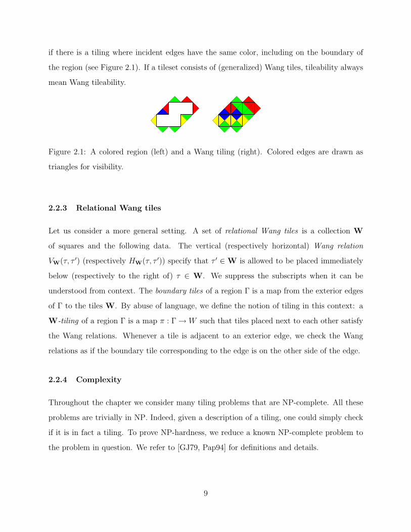
if there is a tiling where incident edges have the same color, including on the boundary of

the region (see Figure 2.1). If a tileset consists of (generalized) Wang tiles, tileability always

mean Wang tileability.

Figure 2.1: A colored region (left) and a Wang tiling (right). Colored edges are drawn as

triangles for visibility.

2.2.3 Relational Wang tiles

Let us consider a more general setting. A set of relational Wang tiles is a collection W

of squares and the following data. The vertical (respectively horizontal) Wang relation

VW(τ, τ ′) (respectively HW(τ, τ ′)) specify that τ ′ ∈W is allowed to be placed immediately

below (respectively to the right of) τ ∈ W. We suppress the subscripts when it can be

understood from context. The boundary tiles of a region Γ is a map from the exterior edges

of Γ to the tiles W. By abuse of language, we define the notion of tiling in this context: a

W-tiling of a region Γ is a map π : Γ→ W such that tiles placed next to each other satisfy

the Wang relations. Whenever a tile is adjacent to an exterior edge, we check the Wang

relations as if the boundary tile corresponding to the edge is on the other side of the edge.

2.2.4 Complexity

Throughout the chapter we consider many tiling problems that are NP-complete. All these

problems are trivially in NP. Indeed, given a description of a tiling, one could simply check

if it is in fact a tiling. To prove NP-hardness, we reduce a known NP-complete problem to

the problem in question. We refer to [GJ79, Pap94] for definitions and details.

9

We will embed Cubic Monotone 1-in-3 SAT as a tiling problem. LetX = x1, . . . , xn

be a set of boolean variables. A (monotone 1-in-3) clause C is a set of three variables. A

(cubic monotone 1-in-3) expression E is a finite collection C of monotone 1-in-3 clauses,

where each variable xi ∈ X occurs three times. We say such E is (1-in-3) satisfiable if there

is an assignment of boolean values 0, 1 to the variables xi ∈ X such that each clause in E

contains precisely one variable receiving 1 (and thus two variables receiving 0).

Cubic Monotone 1-in-3 SAT

Instance: Set X of variables, cubic monotone expression E.

Decide: Whether E is 1-in-3 satisfiable?

The following result was shown by Gonzalez in the language of exact covers:

Theorem 2.2.3 ([Gon85]) Cubic Monotone 1-in-3 SAT is NP-complete.1

We will reduce Cubic Monotone 1-in-3 SAT to a tiling problem Simply Connected

T-Tileability for some fixed T.

2.2.5 Counting problems

Throughout the chapter we consider natural counting problems corresponding to the decision

problems. For example, instead of asking whether satisfying assignments exist, we ask how

many satisfying assignments there are. Similarly, for tileability, we count the number of

tilings. If in the proof of NP-completeness, the corresponding reductions give a bijection

between the sets of solutions, we call such reduction parsimonious.

Parsimonious reductions have the additional benefit of proving counting results using the

same reduction. The class #P consists of the counting problems associated with decisions

problems in NP. A counting problem is #P-complete if it is in #P and every #P question

1Given an expression E, we can associate a bipartite graph G with vertex set X t C, where a variablex ∈ X is adjacent to a clause C ∈ C if x ∈ C. Moore and Robson showed something stronger in [MR01],that this problem is NP-complete even if we require the associated graph to be planar. They did this byreducing from Planar 1-in-3 SAT, which is NP-complete [Lar93, MR08]. However, we do not need to usethe planar version.

10

can be reduced to it. Thus, if there is a parsimonious reduction from problem Q1 to Q2, then

if Q1 is #P-complete, then so is Q2. We refer to [Val79b] (see also [Pap94]) for definitions

and details on #P complexity class.

One main goal is to reduce Cubic Monotone 1-in-3 SAT to a tiling problem Simply

Connected T-Tileability for some fixed T. This reduction will turn out to be parsi-

monious, hence the number of satisfying assignments of a given instance of the satisfiability

problem can be calculated by counting the number of tilings of the transformed instance.

However, it is not known whether the associated counting problem #Cubic Monotone

1-in-3 SAT is #P-complete. To get the #P-completeness result in Theorem 2.1.2, we will

modify the reduction to use 2SAT instead, whose associated counting problem #2SAT is

#P-complete.

2.3 Reduction lemmas

2.3.1 Basic reductions

In this section we consider five classes of Tileability problems. Let T be a collection of

tiles and R be a collection of regions. A decision problem in (T ,R)-Tileability consists

of a fixed tileset T ⊂ T , receives some Γ ∈ R as input, and outputs whether Γ is T-tileable.

We say (T ,R)-Tileability is linear time reducible to (T ′,R′)-Tileability if for any

finite tileset T ⊂ T , there exists a finite tileset T′ ⊂ T ′ and a reduction map f : R → R′

that is computable in linear time (in the complexity of Γ ∈ R), such that Γ ∈ R is T-

tileable if and only if f(Γ) is T′-tileable.2 If, moreover, that (T ′,R′)-Tileability is linear

time reducible to (T ,R)-Tileability, then they are linear time equivalent. Note that the

transformation of the tilesets need not be efficient nor bijective.

For instance, if T is the collection of all rectangular tiles and R consists of simply

connected regions, then (T ,R)-Tileability is a class of problems regarding tiling simply

2Recall that the tiles in the input are given as collections of unit squares.

11

connected regions with rectangular tiles. To simplify the notation, we drop the prefix in

(T ,R)-Tileability when the sets T and R are understood.

Lemma 2.3.1 (Tileability Equivalence Lemma) The following classes of Simply Con-

nected Tileability problems are linear time equivalent:

(i) Tileability with a fixed set of rectangular tiles.

(ii) Tileability with a fixed set of polyomino tiles.

(iii) Tileability with a fixed set of generalized Wang tiles.

(iv) Tileability with a fixed set of Wang squares.

(v) Tileability with a fixed set of relational Wang tiles.

Moreover, the size of the tileset can be preserved in the reductions between (ii) and (iii).

Proof. The reductions (i)⇒(ii)⇔(iii)⇒(iv)⇒(v) are elementary and given below. The re-

duction (v)⇒(i) is stated separately as Lemma 2.3.3 and proved in the next section.

We may consider a rectangular tile as a polyomino tile, which in turn is a monochromatic

generalized Wang tile. Therefore the reductions (i)⇒(ii)⇒(iii) are immediate, where each

reduction map is simply the identity.

(iii)⇒(iv). Given a set of generalized Wang tiles, color each interior edge with a new color

not used anywhere else, and consider each square as a separate Wang square (see Figure 2.2).

These tiles are forced to reassemble themselves as the original generalized Wang tiles. The

reduction map is again the identity.

Figure 2.2: From generalized Wang tiles to Wang squares.

12

(iv)⇒(v). It is obvious how to define the Wang relations to mimic the colored Wang tiles

without increasing the number of tiles. To encode the boundary conditions, we may need

to introduce less than 4χ tiles, where χ is the number of colors permitted on the boundary.

Indeed, to specify a color c on the top boundary, we need to choose an (arbitrary) tile whose

bottom color is c. If no such tile exists, we must add a new tile to do so. If we do not

involve the new tile in any Wang relations in the other directions, then it will never be used

in the actual tiling, and thus will not affect tileability. We do the same for the other three

directions.

The final reduction (v)⇒(i) is more difficult and is the content of Lemma 2.3.3 and proved

in a later section.

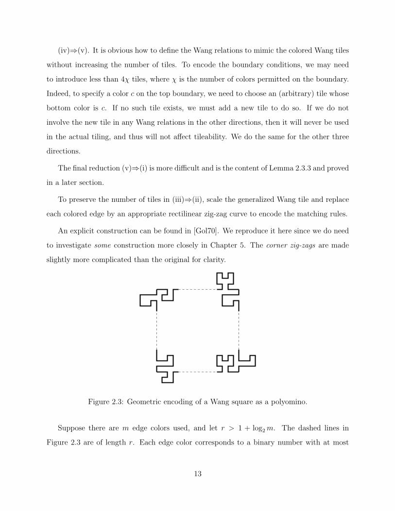
To preserve the number of tiles in (iii)⇒(ii), scale the generalized Wang tile and replace

each colored edge by an appropriate rectilinear zig-zag curve to encode the matching rules.

An explicit construction can be found in [Gol70]. We reproduce it here since we do need

to investigate some construction more closely in Chapter 5. The corner zig-zags are made

slightly more complicated than the original for clarity.

Figure 2.3: Geometric encoding of a Wang square as a polyomino.

Suppose there are m edge colors used, and let r > 1 + log2m. The dashed lines in

Figure 2.3 are of length r. Each edge color corresponds to a binary number with at most

13

r digits. These digits are used to modify the dashed line segments. A digit 0 makes no

modification, while a digit 1 adds a square outward in the corresponding position on the

bottom and right, and removes a square inward along the top and left.

The zig-zags on the corners force these tiles to align in a (dilated) square lattice grid.

Note that even if rotations and reflections are allowed, the corner zig-zags moreover force all

the tiles to have the same orientation. Thus we could in fact allow all isometries when tiling

by polyominoes. This fact is used in the proof of Corollary 5.3.4. When these polyominoes

are adjacent, the series of one-square modifications on the touching boundaries enforce the

color matching rules. This construction clearly works for tiling finite or cofinite regions

instead of the plane as well.

2.3.2 Two main reductions

Lemma 2.3.2 (First Reduction Lemma) There exists a set T of at most 23 general-

ized Wang tiles with total area 133 and using 9 colors such that Simply Connected T-

Tileability is NP-complete. Moreover, this will be achieved by a parsimonious reduction

from Cubic Monotone 1-in-3 SAT.

Lemma 2.3.3 (Second Reduction Lemma) For a set W of at most k Wang squares with c

(boundary) colors, there exists a set R of at most 8(k+4c)2 rectangular tiles with the following

property. Given a simply connected colored region Γ, there is a simply connected region

Γ′ such that Γ is W-tileable if and only if Γ′ is R-tileable. Moreover, this reduction is

parsimonious and can be computed in linear time.

We may transform the set of 23 generalized Wang tiles afforded by Lemma 2.3.2, according

to the procedure outlined in (iii)⇒(ii) of Lemma 2.3.1, in order to obtain Theorem 2.2.2

using 23 polyomino tiles. Similarly, using the transformation of Lemma 2.3.3, we conclude

the result for rectangular tiles in Theorem 2.1.1 (see Subsection 2.6.1). Theorem 2.1.2 can

be shown by modifying the proof of Lemma 2.3.2 to achieve a parsimonious reduction from,

say, 2SAT, whose associated counting problem is #P-complete (see Subsection 2.6.2).

14

2.4 Proof of the First Reduction Lemma (Lemma 2.3.2)

2.4.1 General setup

The goal of this section is to construct a set of generalized Wang tiles that could be used

to solve Cubic Monotone 1-in-3 SAT. Each expression will be encoded as a colored

rectangular boundary. Tiles corresponding to variables and clauses will appear on the left

and right sides of the region, respectively. The variable tiles will “transmit” its state (0 or 1)

through “wires” to the clause tiles; each clause tile will “check” if precisely one out of three

signals it receives is 1. The path of the transmissions will be regulated by placing “crossover

tiles” that allow signals to crossover at specific locations. The positioning of such tiles will

be enforced by using a combination of “control tiles” that follow instructions encoded on the

boundary. Empty spaces will be filled by “filler tiles.”

2.4.2 Tileset T

Let T be a tileset with the 7 small tiles shown in Figure 2.4 and the 3 big tiles in Figure 2.5.

Some horizontal edges are colored by their labels; all unlabeled edges are colored by 0, which

is omitted in the figures for clarity, but acts as any other ordinary color.

4

1

1

(a) left tile L

4

4

2

2

(b) weak tile W

4

4

2

2

6

6

(c) strong tile S

4

3

3

6

(d) right tile R

5

5

8

62

(e) bottom tile B

8

3

5

(f) corner tile K

8

8

(g) filler tile F

Figure 2.4: Tiles in tileset T.

15

5

61

8

(a) crossover tile X

7

7

(b) variable tile V

7

7

(c) clause tile C

Figure 2.5: More tiles in T.

2.4.3 Tileset T′

Recall that the vertical edges of our tiles in T are all colored with 0. Form T′ by recoloring

the vertical edges of tiles in T as follows. Given each small tile τ ∈ T in Figure 2.4, we

introduce a variant by coloring all its vertical edges with 1. The color of the vertical edges

is called the parity of τ . Include both this variant and the original in T′.

Given a rectangular array of these tiles, the parities are consistent across each row and

are independent across the columns. Intuitively, these tiles act as wires that can transmit

data (parity of the tile) horizontally across the region.

We continue defining T′. We add three new versions of the crossover tile X as in Fig-

ure 2.6a. Intuitively, this allows the data transmissions to crossover. We also add a variant

of the variable tile V , as in Figure 2.6b, where all the right vertical edges are colored with 1.

The parity of the variable tile corresponds to the truth value assigned to that variable. Fi-

nally, we replace the clause tile C by the three shown in Figure 2.6c, where each tile has one

out of three pairs of left vertical edges colored with 1. Thus T′ consists of 23 tiles.

We will place the variable tiles on the left and the clause tiles on the right. It remains

to send the data from the variables to the correct clauses. We achieve this by specifying

boundary colors to force crossover tiles to appear at the desired locations.

16

1

1

1

1 1

1

1

1

1

1

1

1

1

1

1

15

61

8

5

61

8

5

61

8

X X X

(a) crossover tile X

7

7

1

1

1

1

1

1

V

(b) variable tile

7

7

7

7

7

7

1

1

1

1

1

1

C C C

(c) clause tile

Figure 2.6: Variations of tiles in T.

2.4.4 Reduction construction

Our goal is to embed the decision problem Cubic Monotone 1-in-3 SAT as a tiling prob-

lem. Given a cubic monotone 1-in-3 SAT expression E with variables X = x1, . . . , xn

and clauses C = C1, . . . , Cn, consider it as a permutation σ = σE ∈ S3n in the sym-

metric group on 3n letters as follows. Think of σ as a bijection from the ordered multiset

X ′ = x1, x1, x1, x2, . . . , xn to the ordered multiset C ′ = C1, C1, C1, C2, . . . , Cn, where

each variable and each clause is listed three times. For each xi ∈ Cj, we have σ(xi) = Cj

once. Now identify each multiset with [3n] = 1, 2, . . . , 3n to get σ as a permutation in S3n.

Let si = (i, i + 1) be an adjacent transposition for i ∈ [3n− 1]. Write σ = si1si2 . . . sid as a

product of adjacent transpositions, with d = O(n2).3

Let ck be the color sequence 01(02)k−163. Define a rectangular region Γ = ΓE as follows.

The height of Γ is 6n and the vertical edges are colored with 0. The width is the length of

the color sequence 7ci1ci2 . . . cid07, which is used as the top boundary. The bottom boundary

is 7(08)t07 with the same length as the top boundary. The following result demonstrates the

ability to place the crossover tile X at arbitrary depth of a large rectangular region.

3For illustration purposes, it is often convenient to encode the product of adjacent transpositions usingwiring diagrams, as shown in Figures 2.7a and 2.8a.

17

Sublemma 2.4.1 The region Γ admits a unique T-tiling.

Proof. The left and right sides are forced to be filled with variable and clause tiles, respec-

tively. Now consider the section in between.

For k ≥ 1 and ` ≥ 0, consider a row of tiles LW kS`R (meaning an L tile followed

by a W tiles k times, an S tile ` times, and ending with an R tile). The bottom color

sequence is 01(02)k(62)`63. One easily checks that the unique way to tile the next row is

with LW k−1S`+1R.

If k = 0, we get the case where we have a row LS`R with bottom color sequence 01(62)`63.

The unique way to tile the next row is with XB`K.

The section below will be filled by filler tiles F . Thus every section below ci is filled

uniquely, with the crossover tile X occupying rows i and i+ 1 in the first column.

The above proof is illustrated with two examples in the next subsection.

Corollary 2.4.2 The expression E is satisfiable if and only if ΓE is T′-tileable. Moreover,

the reduction is parsimonious, that is, the number of tilings of ΓE is the number of satisfying

assignments for E.

The corollary follows immediately from the construction given above, and concludes the

proof of Lemma 2.3.2.

2.4.5 Examples of the tiling construction

In Figure 2.7 we show how to place a crossover tile in a special case, corresponding to ex-

pression (x, y, x), (x, y, y). We illustrate the crossings with a wiring diagram and then give

a complete Wang tiling. In Figure 2.8 below we give a bigger example of the wiring diagram

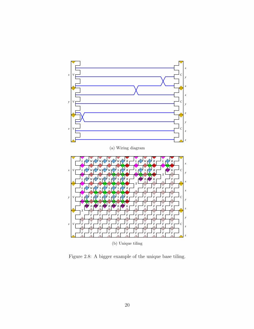
and the unique Wang tiling, corresponding to expression (x, y, x), (x, y, z), (y, z, z).

18

7

7

7

7 7

7

7

7

V

V C

C

x

y

x

x

y

y

y

x

(a) Wiring diagram

7

7

7

7

5

61

8

4

1

1

4

1

1

4

4

2

2

4

4

2

2

6

6

4

3

3

6

4

3

3

6

5

5

8

62

8

3

5

5

61

8

4

1

1

4

3

3

6

8

3

5

8

8

8

8

8

8

8

8

8

8

8

8

8

8

8

8

8

8

8

8

8

8

8

8

8

8

8

8

8

8

7

7

7

7

V

V

X

L

L

W

S

R

R

B K

X

L R

K

F

F F F F

F F F F F

F F F F F

C

C

x

y

x

x

y

y

y

x

(b) Unique tiling

Figure 2.7: A small example of how to place crossover tiles.

2.5 Proof of the Second Reduction Lemma (Lemma 2.3.3)

2.5.1 Basics

In this section, we provide a further connection between Wang tiles and rectangular tiles

(by making a reduction from the latter to the former). Recall that by Lemma 2.3.1, we can

replace generalized Wang tiles with relational Wang tiles.

Without loss of generality, we may assume that the Wang relations are irreflexive, that is,

there is no tile τ such that H(τ, τ) or V (τ, τ). Indeed, suppose W is a set of Wang tiles. Let

W′ = τi : i ∈ 0, 1, τ ∈W be a doubled set of tiles. Define its horizontal Wang relation

as follows. For τ, τ ′ ∈W and i, j ∈ 0, 1, let HW′(τi, τ′j) if and only if HW(τ, τ ′) and i 6= j.

Its vertical Wang relation is defined analogously. It is clear that the Wang relations of W′

are irreflexive. Moreover, a W-tiling can be made into a W′-tiling by adding subscripts to

the tiles in a checkerboard fashion, while the reverse can be done by ignoring the subscripts.

Of course, the same transformation is done on the boundary tiles as well. Clearly this does

not affect tileability nor the number of such tilings.

From now on, assume we are given a fixed set W of relational Wang tiles whose relations

H and V are irreflexive. Our goal is to produce a fixed set R of rectangular tiles with the

following property: Given any simply connected region Γ with specified boundary tiles, we

19

7

7

7

7

7

7

7

7

7

7

7

7

V

V

V

C

C

C

y

x

z

x

y

x

y

z

z

y

z

x

(a) Wiring diagram

7

7

7

7

4

1

1

4

4

2

2

4

4

2

2

4

4

2

2

4

1

1

4

4

2

2

4

4

2

2

4

4

2

2

4

1

1

7

7

5

61

8

4

4

2

2

6

6

4

1

1

4

1

1

4

4

2

2

4

3

3

6

4

3

3

6

4

4

2

2

6

6

4

4

2

2

6

6

4

4

2

2

6

6

4

4

2

2

4

4

2

2

4

4

2

2

4

4

2

2

6

6

4

4

2

2

6

6

4

4

2

2

6

6

8

8

8

8

4

4

2

2

6

6

4

4

2

2

6

6

4

4

2

2

6

6

4

3

3

6

4

3

3

6

4

3

3

6

5

5

8

62

5

5

8

62

5

5

8

62

5

5

8

62

8

3

5

8

8

8

8

8

8

8

8

8

8

8

8

8

8

8

8

8

8

8

8

8

8

8

8

8

8

8

8

8

8

8

8

5

61

8

4

1

1

4

1

1

4

4

2

2

6

6

4

4

2

2

5

5

8

62

8

3

5

4

3

3

6

4

3

3

6

5

61

8

7

7

7

7

4

1

1

4

3

3

6

8

3

5

8

8

8

8

8

8

8

8

8

8

8

8

8

8

8

8

8

8

8

8

8

8

8

8

8

8

8

8

8

8

8

8

8

8

8

8

8

8

8

8

8

8

8

8

8

8

8

8

8

8 7

7

8

8

8

8

8

8

8

8

V

V

L W W W

L WW

WL

V

X

SL

L

W

R

R

S

S

SW

W

W

S

S S

F

F

S S S

R

R

R

B B B B K

F

F

F

F

F

F

F

F

F

F

F

F

F

FF

F

X

L

L

S

W

B K

R

R

X

C

C

L R

K

F

F

F

F F

F

F

F

F

F

F

F

F

F

F

F

F

F

F

F

F

F

F

F

F

C

F

F

F

F

y

x

z

x

y

x

y

z

z

y

z

x

(b) Unique tiling

Figure 2.8: A bigger example of the unique base tiling.

20

can produce (in linear time) a simply connected region Γ′ such that Γ is W-tileable if and

only if Γ′ is R-tileable. Moreover, the number of W-tilings of Γ will be the same as the

number of R-tilings of Γ′.

For simplicity, we first consider the case where we are given an r × c rectangular region

Γ with specified boundary tiles.

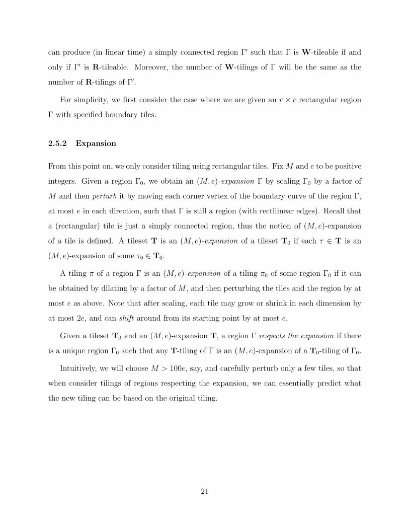
2.5.2 Expansion

From this point on, we only consider tiling using rectangular tiles. Fix M and e to be positive

integers. Given a region Γ0, we obtain an (M, e)-expansion Γ by scaling Γ0 by a factor of

M and then perturb it by moving each corner vertex of the boundary curve of the region Γ,

at most e in each direction, such that Γ is still a region (with rectilinear edges). Recall that

a (rectangular) tile is just a simply connected region, thus the notion of (M, e)-expansion

of a tile is defined. A tileset T is an (M, e)-expansion of a tileset T0 if each τ ∈ T is an

(M, e)-expansion of some τ0 ∈ T0.

A tiling π of a region Γ is an (M, e)-expansion of a tiling π0 of some region Γ0 if it can

be obtained by dilating by a factor of M , and then perturbing the tiles and the region by at

most e as above. Note that after scaling, each tile may grow or shrink in each dimension by

at most 2e, and can shift around from its starting point by at most e.

Given a tileset T0 and an (M, e)-expansion T, a region Γ respects the expansion if there

is a unique region Γ0 such that any T-tiling of Γ is an (M, e)-expansion of a T0-tiling of Γ0.

Intuitively, we will choose M > 100e, say, and carefully perturb only a few tiles, so that

when consider tilings of regions respecting the expansion, we can essentially predict what

the new tiling can be based on the original tiling.

21

2.5.3 Rectangular tiles R0 and the region Γ0(r, c)

Consider the following tileset:

R0 = f = R(34, 11), w = R(31, 14), s = R(10, 10), h = R(11, 31), v = R(14, 34) ,

where R(a, b) denotes a rectangle of height a and width b (see Figure 2.9). For a rectangle

t, write ht t and wd t for its height and width, respectively.

f

(a)

w

(b)

s

(c)

h

(d)

v

(e)

Figure 2.9: Rectangular tiles R0: (a) fixed rectangle f , (b) fixed rectangle w, (c) flexible

square s, (d) flexible rectangle h, and (e) flexible rectangle v.

Now consider the region Γ0(r, c) defined as follows (see Figure 2.10). On each vertical

side, there are r protrusions of height hth and width wd s, separated by height ht f . On

each horizontal side, there are c cavities of width wd v and height ht s, separated by width

wd f .

wd s

hht

sht

wd f

wd v

fht

Figure 2.10: Boundary region Γ0(2, 2).

Sublemma 2.5.1 The unique R0-tiling of Γ0(r, c) consists of r rows and c columns of the

w tile.

22

Proof. Fix natural numbers a = 10 and b = 1. The tiles introduced above can now be

written as f = R(3a + 4b, a + b), w = R(3a + b, a + 4b), s = R(a, a), h = R(a + b, 3a + b),

and v = R(a+ 4b, 3a+ 4b).

We begin with a few definitions. A horizontal (vertical) segment of a region is called

bounded if the region extends downward (to the right) on both sides of the segment. For

t ∈ v, h, a pair (t, s) is the configuration of placing the tile s above or below t, aligned

on the left. The orientation of the pair is positive (negative) if s is placed below (above).

Similarly, for t ∈ w, f, a pair (t, s) is obtained by placing s to the left or right of t, aligned

on top. The orientation is positive (negative) if s is placed to the right (left). A bounded

segment is tiled by a tile (pair) if in all tilings, the tile (pair) is adjacent to the segment.

We will tile the region Γ0(r, c) in steps, as indicated by the numbers labeled on Figure 2.11.

Note that since a > b, each bounded horizontal segment of width wd f on the top border

must be tiled by f tiles, labeled 1. Similarly on the left, the bounded vertical segments of

height hth must be tiled by h tiles, labeled 2. This creates a bounded vertical segment of

height ht v+ ht s on the top left corner; since a > 3b, it is tiled by the pair (v, s), labeled 3.

Since a > 4b, it is obvious that it needs to be positively oriented, to avoid a hole of width

wd v −wd s and height ht s, which cannot be filled.

Note that since a > 3b, this creates a new bounded horizontal segment of width wdw +

wd s, which is tiled by the pair (w, s), labeled 4. If w is on the left, it will create a bounded

horizontal segment of width wd f + wd s to its left. Otherwise, if w is on the right, several

s will be forced to appear on the left and still create the same bounded segment. Therefore,

the (w, s) pair creates the bounded segment, regardless of how it is oriented.

Since a > 3b, this bounded horizontal segment of width wd f + wd s is again tiled by

an (f, s) pair, labeled 5. Like the (v, s) pair above, since a > 4b, this needs to be positively

oriented. This creates the bounded vertical segment of height ht v + ht s, tiled by a pair

(v, s), labeled 6, as above. In either orientation, it bounds the vertical segment of height

htw above, concluding that the (w, s) pair (labeled 4) we placed above needs to be positively

oriented. Furthermore, this bounds the vertical segment of height hth + ht s, again tiled

23

h

v

s

f w

1 1 1

2

2

3

3

4

4

5

5

6

6

7

7

8

8

9

9

10

10

11

11

12

12

13

14

14

15

15

16

16

17

18

18

19

19

20

21

21

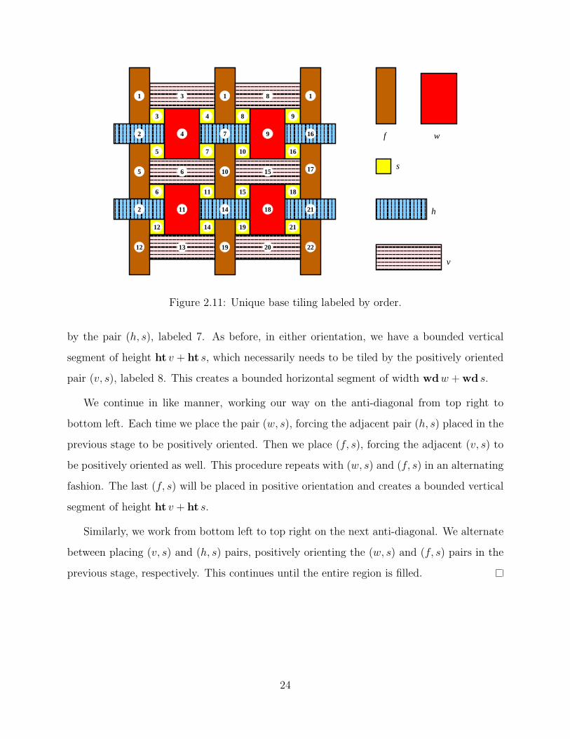
22

Figure 2.11: Unique base tiling labeled by order.

by the pair (h, s), labeled 7. As before, in either orientation, we have a bounded vertical

segment of height ht v + ht s, which necessarily needs to be tiled by the positively oriented

pair (v, s), labeled 8. This creates a bounded horizontal segment of width wdw + wd s.

We continue in like manner, working our way on the anti-diagonal from top right to

bottom left. Each time we place the pair (w, s), forcing the adjacent pair (h, s) placed in the

previous stage to be positively oriented. Then we place (f, s), forcing the adjacent (v, s) to

be positively oriented as well. This procedure repeats with (w, s) and (f, s) in an alternating

fashion. The last (f, s) will be placed in positive orientation and creates a bounded vertical

segment of height ht v + ht s.

Similarly, we work from bottom left to top right on the next anti-diagonal. We alternate

between placing (v, s) and (h, s) pairs, positively orienting the (w, s) and (f, s) pairs in the

previous stage, respectively. This continues until the entire region is filled.

24

2.5.4 Expansion R of R0

We will now define a clever set of perturbed expansion tiles that will correspond to the rela-

tional Wang tiles. Only the tiles s, h, and v will have perturbations. Let W = τ1, . . . , τn

be the fixed set of relational Wang tiles with irreflexive horizontal and vertical Wang rela-

tions H and V , respectively. Fix e = 5n and M = 100e for the remainder of the section. Let

R be an (M, e)-expansion of R0 as follows:

For t ∈ s, h, v, let t(a, b) be the scaled version of t with height and width increased by

a and b, respectively. Imagine that the h and v tiles can stretch horizontally and vertically,

respectively, and the s tiles can stretch in both directions. Then the w tiles, having no

perturbations, will only shift around a little (by at most e). The f tiles will stay fixed,

enforcing the global structure. See Figure 2.12. A w tile will be shifted to the right and

down by 5i to represent the Wang tile τi. To restrict the shifts to only those sizes, we replace

s with the appropriate perturbed versions. Namely, for each i, introduce four tiles with

perturbations s(±5i,±5i), where all four combinations of signs are included. To enforce

the Wang relations, for each τi, τj ∈ W such that V (τi, τj) or H(τi, τj), we introduce the

perturbation v(5j − 5i, 0) or h(0, 5j − 5i), respectively. This is the set R we will use.

τ

τj

i

Figure 2.12: Shifting an expansion of the unique tiling to represent Wang tiles.

25

2.5.5 Rectangular tiling

Obtain an (M, e)-expansion Γ(r, c) of Γ0(r, c) by scaling with a factor of M and then per-

turbing it as follows. Recall that there are r protrusions on each vertical side and c cavities

on each horizontal side. Each protrusion or cavity corresponds to a boundary tile of Γ in a

natural way. Perturb the protrusion or cavity to the right or down, respectively, by 5i units

if it corresponds to τi.

Sublemma 2.5.2 The (M, e)-expansion Γ(r, c) of Γ0(r, c) respects the expansion R of R0.

Proof. Recall the argument in the proof of Sublemma 2.5.1. As the inequalities are all

satisfied, the f tiles are fixed and force the perturbations to stay local. The w tiles have two

degrees of freedom. They can move ±5i in each direction, as regulated by the s tiles. Now

note that the inequalities in the proof of Sublemma 2.5.1 are preserved. We leave the (easy)

details to the reader.

We now return to the proof of Lemma 2.3.3. It is clear that given a Wang W-tiling of

the rectangle Γ with boundary, we will get an R-tiling of Γ(r, c). Indeed, simply take the

unique tiling of Γ0(r, c) as afforded by Sublemma 2.5.1, scale by a factor of M , and then

shift each w tile to the right and down by 5i if it represents τi, and adjust the other tiles in

the obvious way.

Conversely, if we are given an R-tiling of Γ(r, c), we wish to recover the W-tiling of

Γ. This is achieved using the following two sublemmas, both of which are clear when all

numbers are considered in base 5; we omit the (easy) details.

Sublemma 2.5.3 The equation 5i − 5j = 5k + 5` does not admit a solution in N.

Therefore each w tile will shift to the right and down (as opposed to shifting left or up),

and hence indeed represents a Wang tile τi for some i.

Sublemma 2.5.4 The equation 5i − 5j = 5k − 5` does not admit solutions in N except if

i = j or i = k.

26

If a w tile representing τj is to the right of a w tile representing τi, then h(0, 5j − 5i)

must be in R. By the sublemma above, the differences 5j − 5i are all distinct (recall that

the Wang relations are irreflexive, so i = j does not happen), therefore we must have had

H(τi, τj) as part of the Wang relation. Similarly for the vertical Wang relation V . So by

reading off the associated tile τi from the shifts of each w tile, we get a Wang W-tiling of Γ.

This completes the construction of Γ0(r, c) for the case when Γ is a rectangle. For the

general case, when Γ is a simply connected region, the proof follows verbatim after replacing

Γ(r, c) and Γ0(r, c) by appropriate regions.

It remains to get the upper bound estimates on the number of rectangles involved in

the construction. Suppose we are given a set of k Wang squares using c colors (on the

boundary). By Lemma 2.3.1 we can equivalently consider a set of less than k+ 4c relational

Wang tiles. To satisfy irreflexivity, we might need to double the set of tiles, resulting in

n = |W| < 2(k + 4c) tiles. When making R, we will have one each of f and w tiles. There

will be 4n perturbed s tiles and at most n2 perturbed h and v tiles each. In total,

|R| ≤ 2n2 + 4n+ 2 = 2(n+ 1)2 ≤ 8(k + 4c)2.

This concludes the proof of Lemma 2.3.3.

2.6 Proof of theorems

2.6.1 Proof of Theorem 2.1.1

In the proof of Lemma 2.3.2 in Section 2.4, we constructed the set W of 23 generalized

Wang tiles using 9 colors, such that Simply Connected W-Tileability is NP-complete.

It remains to count the total number of rectangles we obtain from the series of reduction

constructions.

First, compute the number of Wang squares given by the transformation in Lemma 2.3.1.

Observe that the total area of tiles in W is 9 · 5 + 8 · 4 + 4 · 14 = 133. Therefore we can

break them into 133 Wang squares by adding 133− 23 more colors. But as these colors do

27

not appear on the boundary, they need not be counted. Hence, in Lemma 2.3.3, we can take

k = 133 and c = 9, thus giving us at most 106 rectangles.

2.6.2 Proof of Theorem 2.1.2

First, note that the reduction in the proof of Theorem 2.1.1 is parsimonious. However, there

seems to be no #P-completeness result for the #Cubic Monotone 1-in-3 SAT problem.

This is easy to fix by making a similar reduction from the 2SAT problem, whose associated

counting problem is #P-complete (see [Val79b]).

An instance of 2SAT is a set of variables and a collection of clauses. Each clause is

a disjunction of two literals, where each literal is either a variable or a negated variable.

The problem is to decide whether there is a satisfying assignment such that each clause has

at least one true literal. We modify the proof of Lemma 2.3.2 to obtain a parsimonious

reduction from 2SAT. By replacing the two variations of the variable tile by the ones shown

in Figure 2.13a, we may set up unnegated and negated copies of a single variable. Indeed,

with a sequence of 5(26)r−136(26)s−14 as colors on the left vertical edge, we create a list of

r + s variables, where the last s are negated. By replacing the three variants of the clause

tile by the three obvious candidates in Figure 2.13b, we force each clause to be satisfied.

61

11

67

5

11

75

2

21

11

31

31

1

47

47

11

(a) tiles for variables

1

7

7

1

7

7

1

1

7

7

1

1

1

1

(b) clause tiles

Figure 2.13: Tiles for 2SAT.

Note that the modified tileset has a smaller total area, and has the same number of colors

used on the boundary. Therefore as in the proof of Theorem 2.1.1, we apply Lemma 2.3.3

to conclude that 106 rectangles suffice.

28

2.7 Final remarks and open problems

2.7.1

Theorem 2.2.1 was only announced in [GJ79], referencing an unpublished preprint. Of course,

now we have much stronger results.

A version of Lemma 2.3.2 was first announced in Levin’s original 1973 short note on NP-

completeness [Lev73], but the proof has never been published.4 Although we were unable

to find in the literature an explicit construction for either Lemma 2.3.2 or, equivalently,

of Theorem 2.2.2, we do not claim this result as ours, since it became a folklore decades

ago. We include the proof for completeness, and since we need an explicit construction. An

alternative proof is outlined in Subsection 2.7.2 below.

Let us mention that using [Oll09], the number of tiles in Theorem 2.2.2 can be reduced

to 11, but this reduction has no effect on the number of tiles in the main theorems. Indeed,

Theorem 2.2.2 is an immediate corollary of Lemma 2.3.2, which is the one needed in the

proof of main theorems 2.1.1 and 2.1.2.

2.7.2

Our proof of Lemma 2.3.2 is completely elementary and yields explicit bounds (see also

Subsection 2.7.1). Let us sketch an alternate proof of the lemma, using a non-deterministic

universal Turing machine (UTM). It was suggested to us by Cris Moore.

Fix some non-deterministic universal Turing machine M. Given two finite tape configu-

rations and a natural number t (in unary), it is NP-complete to decide whether M transforms

the first tape configuration to the second with t steps of computation. Fix a finite set W

of Wang tiles that simulate the space-time computation diagram of M (see Section 6.1).

Encode the given tape configurations as the top and bottom boundaries of a rectangular

region with height t. This region is tileable by W if and only if M transforms the first

4Leonid Levin, personal communication.

29

tape configuration to the second in precisely t steps. The details are straightforward (see

e.g. [LP97, §7]).

Note that this method also proves the counting result. Indeed, one can devise a UTM so

that there is a bijective correspondence between the accepting paths of the UTM and of the

Turing machine it is simulating.

We do not know if this approach leads to improvements in the number of Wang tiles in

the lemma, as this would depend on the smallest UTM. Given an m-state n-symbol Turing

machine with k instructions, the standard construction of Wang tiles to simulate such a

Turing machine yields more than nm + n + k tiles. As a perspective, among the smallest

known UTMs, this minimum is achieved by Rogozhin’s 4-state 6-symbol machine with 22

instructions, which already yields more than 52 tiles [Rog96] (see also [NW09]). Unless a

substantial progress is made in finding small UTMs, our elementary proof still gives better

bounds.

Indeed, the proof of Lemma 2.3.2 constructs a set of 23 generalized Wang tiles (133

Wang squares). However, it is possible to decrease these numbers by elementary means.

After this chapter (as a paper) was written, incremental improvements have led to a set of

117 rectangles. The details are in the next chapter.

2.7.3

In the tiling literature, the original theoretical emphasis was on tileability of the plane, the

decidability and aperiodicity. The problem was often stated in the equivalent language of

Wang tiles [Ber66, Rob71, Wan65]. Unfortunately, there does not seem to be any stan-

dard treatment of the finite Wang tiling problems. Although some equivalences in the

Lemma 2.3.1 are routine, such as the reduction in Figure 2.2, others seem to be new. We

present full proofs for completeness.

30

2.7.4

Historically, finite tilings were a backwater of the tiling theory, with coloring arguments

being the only real tool [Gol65]. On a negative (complexity) side, originally, the tileability

problem was studied for general regions, where the tiles were part of the input. The NP-

completeness of this most general problem is given in [GJ79, §GP13]. When the set of tiles

is fixed, NP-completeness was shown for general regions and various fixed small sets of tiles

(see [MR01] and [BNRR95] building on the earlier unpublished work by Robson).

On the positive side, papers of Thurston [Thu90] and Conway & Lagarias [CL90] intro-

duced the height function and the tiling group interrelated approaches. The key underlying

idea is the use of combinatorial group theory applied to the boundary word of the sim-

ply connected regions, so the tilings become Van Kampen diagrams of the corresponding

tiling group. This approach allowed numerous applications to perfect matchings [Cha96],

tile invariants [Kor04, MP02, Rei03], tileability [She02], various local move connectivity re-

sults [KP04, Rem98], classical geometric problems [Ken96], applications to colorings and

mixing time [LRS01], etc. More relevant to this chapter, the breakthrough result by C. and

R. Kenyon [KK92] proved that tileability with bars of simply connected (s.c.) regions can

be decided in polynomial time. This result was further extended to all pairs of rectangles by

Remila in [Rem05], and by Korn [Kor04] to an infinite family of generalized dominoes. Our

Main Theorem puts an end to the hopes that these results can be extended to larger sets of

rectangles.

Note also that having s.c. regions gives a speed-up for polynomial problems. For example,

domino tileability is a special case of perfect matching, solvable in quadratic time on all

planar bipartite graphs [LP09]. However, Thurston’s algorithm is linear time (in the area),

for all s.c. regions (see [Cha96, Thu90]).

31

2.7.5

We conjecture that in the Main Theorem (Theorem 2.1.1), the number of rectangles can be

reduced down to 3, thus matching the lower bound (Remila’s tileability algorithm for the

case of two rectangles). As a minor supporting evidence in favor of this conjecture, let us

mention that the proofs in [KK92, Rem05] are crucially based on local move connectivity,

which fails for three general rectangles. In the absence of algebraic methods, there seem to

be no other (positive) approach to tileability.

2.7.6

This result of Main Theorem can be contrasted with a large body of positive results on tiling

rectangular regions with a fixed set of rectangles.

Theorem 2.7.1 (“Tiling rectangles with rectangles” Theorem [LMP05]) For every finite

set R of rectangular tiles, the tileability problem of an [M × N ] rectangle can be decided in

O(logM + logN) time.

Note that Theorem 2.7.1 has linear time complexity for the rectangular regions written

in binary. This result is based on the pioneer results by Barnes [Bar82a, Bar82b] applying

commutative algebra, the finite basis theorem [DK75] (see also [Rei05]), and the transfer

matrix method (see e.g. [Sta97, Ch. 4]).

It seems, tilings of rectangles have additional structure, which general regions do not

have. See e.g. [BSST40, CGG+82, Rob82] for assorted results on the subject. On the other

hand, when the tiles are part of the input, deciding tileability can be NP-hard, and the proof

can be used to show that counting tilings is #P-hard. Note that the results in [LMP05] only

discuss tileability, not counting. It would be interesting to obtain general results on the local

move connectivity and hardness of counting results for tilings of rectangular regions with

rectangles.

32

2.7.7

Although counting perfect matchings in general graphs is #P-complete, for the grid graphs a

Pfaffian formula gives a count for the number of domino tilings for any (not necessarily simply

connected) region; this formula can be applied in polynomial time [LP09] (see also [Ken04]).

In a different direction, Moore and Robson [MR01] conjecture that already for two bars, the

problem is #P-complete for general regions. They note that the corresponding reductions

in [BNRR95, MR01] are not parsimonious. Thus, until now, the #P-completeness was open

for any finite set of rectangular tiles, even for general regions.

We make a stronger conjecture that for every tileset T of two bars [1 × k] and [` × 1],

where k, ` ≥ 2, (k, `) 6= (2, 2), the counting of tilings by T of simply connected regions

is #P-complete. In particular, the number 106 in Theorem 2.1.2 can be decreased to 2.

There is no direct evidence in favor of this, except that the general combinatorial counting

problems tend to be #P-complete unless there is a special algebraic formula counting them.

Furthermore, when it comes to tile counting, there seem to be no direct benefit of simple

connectivity of the regions, so such result is likely to be equally hard as for general regions.

We refer to [Jer03] for the introduction and references.

2.7.8

By a simple modification of the Wang tiles, we can also get a parsimonious reduction

from SAT. For that, first, we can introduce wire splitters and the NOT gate. By doing

so, we remove the “cubic” and “monotone” constraints, respectively. These would play the

same role as crossover tiles, and require a separate color on the boundary for each. This

would also increase the set of tiles by introducing new variants for the V and L tiles as well.

We omit the details.

We can then introduce the AND gate in a similar fashion, again with a new control color

on the top and new versions of the V , C and L tiles. This gives the embedding of SAT.

33

This reduction is parsimonious in the same way as the reduction in Theorem 2.1.2, which

implies that the associated counting problem is also #P-complete.

Let us compute the total number of rectangles necessary for this construction. First, this

would increase the number of Wang tiles from 23 to no more than 23 · 8. Then, the same

argument as above gives the 108 bound in the number of rectangular tiles. We omit the

(easy) calculation and details.

2.7.9

The reductions in this chapter can be used to prove uniqueness results on tileability with

rectangles, i.e. whether there exists a unique tiling of a region with a given set of rectangular

tiles. In [BNRR95], the problem was completely resolved in the case of two bars. An even

simpler solution follows from [KK92] in this case. Since all tilings are local move connected,

taking the “minimal tiling” constructed by the algorithm in [KK92] and trying all potential

moves gives an easy polynomial time test. More generally, Remila [Rem05] showed that for

two general rectangles one can go from one to another with certain non-local moves which

are easy to describe. Again, since he produces the “minimal tiling,” his algorithm can be

used to decide unique tileability with two rectangles.

Now, our approach, via reduction from the general SAT problem (see above) shows that

for a certain finite set of rectangles, uniqueness of tilings of a simply connected region is

as hard as UNIQUE SAT, which is co-NP-hard and has been extensively studied [BG82,

VV86]. This seems to be the first result of this type.

2.7.10

Although Theorem 2.7.1 extends directly to bricks in higher dimensions [LMP05], this is an

exception rather than the rule. In fact, in Chapter 4, we show that almost no other positive

tileability results extend to higher dimensions, even Thurston’s algorithm mentioned above.

34

CHAPTER 3

Reducing the number of rectangles

In the previous chapter, we established that a bound of 106 suffices to find a fixed set

of rectangles R such that the tileability problem of simply connected regions with R is

NP-complete. In this chapter, we will incrementally reduce this number by incorporating

various ideas. Obvious places of attack include optimizing the Wang tileset construction in

Lemma 2.3.2 and the bound in the Second Reduction Lemma (Lemma 2.3.3).

3.1 Improving the Wang tileset

The generalized Wang tileset W15 consists of Vi, Li, Ri, and Fi, for i ∈ 0, 1, Xij for

i, j ∈ 0, 1, and Ci for i ∈ 1, 2, 3 (see Figure 3.1, where δi,j is the Kronecker delta, 1 if

i = j and 0 otherwise). When referring to a tile, we may suppress the subscript for notational

convenience.

Note that a color sequence of `okr on the top boundary will conjure a crossover tile X to

appear in row k + 1 below the color `. Using these, we can follow the same general setup

as before to embed a cubic monotone 1-in-3 SAT expression. Indeed, create a rectangular

region of height 3n, where n is the number of variables. Color the left, right, and bottom

boundaries by `, r, and o, respectively.

This means that there will be n variable tiles on the left, each either V0 or V1, denoting

whether the variable is false or true, respectively. The L, R, F tiles all transmit data hor-

izontally, as before. The X tiles will appear at predefined locations, causing the signals to

crossover. Finally, the n clause tiles C on the right will check 1-in-3 satisfaction.

35

Vi

`

`

`

i

i

i

o

o

(a) Tile Vi.

Ci

δi,1

δi,2

δi,3 r

r

r

o

o

(b) Tile Ci.

Xiji

j

j

i

` r

o

o

(c) Tile Xij .

i

`

`

iLi

(d) Tile Li.

i

o

o

iFi

(e) Tile Fi.

Rii i

r

r

o

o

(f) Tile Ri.

Figure 3.1: Tiles for constructing W15.

This proves the following lemma, improving the previous construction of 23 generalized

Wang tiles.

Lemma 3.1.1 There exists a set W15 of at most 15 generalized Wang tiles such that Simply

Connected T-Tileability is NP-complete.

This directly leads to an improvement of Theorem 2.1.1.

Theorem 3.1.2 There exists a finite set R15 of at most 20808 rectangular tiles, such that

the tileability problem of simply connected regions with R15 is NP-complete.

Proof. The total area of W15 is 3 ·9+2 ·2+1 ·4 = 35, thus we may take k = 35 (the number

of Wang squares) and c = 4 (the number of boundary colors) in Lemma 2.3.3 to get a set

R15 of at most 20808 rectangular tiles.

36

3.2 Improving the Second Reduction Lemma

What follows is a second version of the Second Reduction Lemma (Lemma 2.3.3).

Lemma 3.2.1 (Second Second Reduction Lemma) For a set W of at most k Wang squares

with c colors, there exists a set R of at most 2k + 8 mink, c2+ 3 rectangular tiles with the

following property. Given a simply connected colored region Γ, there is a simply connected

region Γ′ such that Γ is W-tileable if and only if Γ′ is R-tileable. Moreover, this reduction

is parsimonious and can be computed in linear time.

In particular, this gives a linear bound 10k + 3, which is a big improvement over the

previous quadratic bound 8(k + 4c)2. Note that here c is the number of colors, not just the

boundary colors as in the original Second Reduction Lemma 2.3.3. Another distinction is

that the Wang tiles here are not relational.

Proof. First assume that each Wang tile does not have monochromatic parallel edge pairs,

and follow the proof of the original Second Reduction Lemma and take the same R0 as

constructed in Section 2.5. Let R′ be a different (M, e)-expansion of R0 as follows:

The tiles f , h, and v will have no perturbations. Suppose the Wang tiles have colors

1, 2, . . . , c. For each Wang tile with colors N , E, S, W on the north, east, south, and

west sides, respectively, denoted τ(W, NS, E), introduce a perturbed w tile w(5S − 5N , 5E −

5W ). Furthermore, introduce four perturbed s tiles s(−5N , 5W ), s(−5N ,−5E), s(5S, 5W ),

and s(5S,−5E). This finishes the construction.

Instead of having a single w tile shift 5i to the right and down to indicate tile τi, we shift

the h and v tiles 5i to the right and down, respectively, to indicate color i on the edge of the

two adjacent Wang tiles. Given a colored [r× c] rectangular region, let Γ(r, c) be an (M, e)-

expansion of Γ0(r, c), obtained by perturbing the protrusions and the cavities corresponding

to color i on the boundary by 5i to the right and down, respectively (cf. Section 2.5).

37

It is easy to see that if we are given a Wang tiling, we can place all the h and v tiles by

shifting them the appropriate amounts from the base tiling, and then filling in the w and s

tiles, which are, by construction, available to fill the gaps precisely.

Conversely, if there is a rectangular tiling, Sublemma 2.5.3 implies that the h and v will

always shift to the right or down only, thus enabling us to color the edges of a Wang tiling

of the rectangular boundary given. Sublemma 2.5.4 implies that the Wang tiles and the w

tiles are in bijective correspondence, hence the Wang tiling obtained above by coloring edges

is indeed a tiling by Wang tiles.

Note that for this argument, a Wang tile cannot have monochromatic parallel edge pairs.

This is analogous to the irreflexivity requirement of the relational Wang tiles. To ensure this,

one can double the set of tiles as follows: replace a Wang tile τ(W, NS, E) by tiles τ(W, N

S′ , E′)

and τ(W ′, N ′

S, E).

Let us count the number of tiles created. We have the three fixed tiles f , h, and v. For

each Wang tile in the doubled set of size 2k, we create a w tile and four perturbed versions

of s. Some of the s tiles may be the same, thus we get an upperbound of 8k. On the other

hand, for the s tiles involving north and west colors, there are at most 2c2 of them, one from

each type of the doubled tiles. Similarly for the other three corners, thus yielding a bound

of 8c2 instead. Combining these gives the desired 2k + 8 mink, c2+ 3 bound.

Corollary 3.2.2 There exists a finite set Rf of at most 353 rectangular tiles, such that the

tileability problem of simply connected regions with Rf is NP-complete.

Proof. Starting with the generalized Wang tiles W15 constructed in Lemma 3.1.1, we break

them into k = 35 Wang squares. The number of colors far exceed√

35, thus we use the

10k + 3 bound from the second Second Reduction Lemma to obtain a set of at most 353

rectangles.

38

3.3 Ad-hoc optimizations

The procedures of the Second Reduction Lemmas work on general sets of Wang tiles. How-

ever, we need only apply to a specific set. Let us consider this carefully to further reduce

the number of rectangles needed.

One obvious waste is the general bound, where we estimate the number of tiles given the

construction. At the end, we will carefully count exactly how many rectangles we obtain.

Recall that for the original Second Reduction Lemma, the Wang tiles must be irreflexive—no

tile is allowed adjacent to itself. To ensure this, we had to double the number of tiles. Sim-

ilarly, in the second Second Reduction Lemma, the Wang tiles cannot have monochromatic

parallel edge pairs. We also doubled the number of tiles to satisfy this requirement. In what

follows, we will modify the set of tiles slightly by hand so no doubling is needed. This will

increase the number of tiles, but not as much as doubling.

Lemma 3.3.1 There exists a set Wa of at most 33 Wang squares, without monochromatic

parallel edge pairs, such that Simply Connected T-Tileability is NP-complete.

Proof. Please refer to Figure 3.2 for the modifications of the L, F, X, and C tiles from W15.

Recall that the setup is for tiles to transmit truth values horizontally from left to right. We

invert the truth values at each column, so the L and the F tile do not have monochromatic

pairs of vertical edges. For easy reading of the truth values of variables, we may use a

rectangle with even width, so the clause tiles will get as input truth values that have been

inverted even number of times (i.e., not at all). The truth inversion setup solves the problem

for the two Xii tiles having monochromatic vertical pairs for the bottom squares, but shifts

the problem to the other two Xij tiles, namely, when i 6= j. Thus we make those tiles [2× 2]

squares with the obvious fourth tile. Namely, the right color of the fourth tile is the same

as the left color of the tile in the top left. To match with what follows, the bottom color of

the fourth tile will be ` instead of the expected o.

39

i

o

`

1− iLi

(a) Tile Li.

Xiii

i

i

1− i

` r

o

o

(b) Tile Xii.

Xi,1−i

i

1− i

1− i

i

` r

o `

(c) Tile Xi,1−i.

i

`

o

1− iFi

(d) Tile Fi.

i

o

`

i′Ci

(e) Tile Ci.

C2

1

0

0′

1

o

o

o `

(f) Tile C2.

Figure 3.2: Tiles for constructing Wa.

As for horizontal edges, the L and the F tiles are the only ones presenting problems. We

replace the top of L by color o and similarly replace the top of F by color `. Now L and F will

occur as alternating sequences in each column. Imagine placing a crossover X tile where we

want it to occur, and putting R tiles diagonally on top of it. We can then fill in the region

above and below with L and F tiles. The top and bottom edges will be alternating sequence

of o and ` colors. They will start as the same sequence if the number of variables is even,

and opposite otherwise. To place a crossover tile with its top in row k, we change one of the

` on the top boundary to r, and change the kth color to its left from ` to o if k is even, and

o to ` if k is odd.

We have removed the need for doubling, yielding a set of 4 · 2 + 3 · 7 + 2 · 2 + 1 · 4 = 37

Wang squares, much better than 35 tiles doubled to 70. We now apply one last ad-hoc trick

to reduce this number further.

Replace the C tiles (accounting for 3 · 3 of the area) with the tiles Ci, i ∈ 0, 1, and C2

that contribute only 5 to the area.

40

0′

0′

1′

o o

o o

o o

Figure 3.3: Right boundary to be used with the Wa tiles.

To use these tiles instead, we replace the right boundary of the rectangle by n copies of

the boundary shown in Figure 3.3. We then extend the bottom boundary of the rectangle

to reach the end of this staircase boundary, using the colors ` and o depending on the

parity of how many squares are above. Namely, the sequence . . . `2o2`2o2`2, comprising of

an alternating sequence of `2 and o2, ending with `2 on the right.

We will start with a rectangle of even width, so as to have the same parity between the

second vertical edge (the right edge of a variable tile) and the penultimate vertical edge (the

left edge of the right-most square) in each row. If the penultimate edge has color i while the

color of the last vertical edge is i′, then tile Ci fits there. Otherwise, C2 allows shuffling a 1

signal down a row, provided that the next row carries a 0 signal. In such a manner, every

three rows will check 1-in-3 satisfaction, as desired.

The space below such a clause region will not be disturbed, and will simply be filled with

L and F tiles. This results in the desired construction of Wa with 33 Wang squares.

We now explicitly count how many rectangles we get when applying the second Second

Reduction Lemma to this carefully constructed tileset Wa.

Theorem 3.3.2 There exists a finite set Ra of 117 rectangular tiles, such that the tileability

problem of simply connected regions with Ra is NP-complete.

Proof. Recall that besides the three tiles (f , h, and v) that do not have perturbations, we

create five types of tiles, listed below in the first column of Table 3.1. We count the number

of new rectangles created due to the introduction of L,F, . . . ,C tiles, in that order. For

41

example, the top and left edges of the left tile of Ri are colored the same as that of Fi, thus

the s(−5N , 5W ) entry for R is 2 instead of 4. We also note that when breaking Xij, i 6= j,

into four Wang squares each, we may color the internal horizontal edge on the right as o,

then the top right corner tile of Xij, i 6= j, is the same as the one for Xjj. That is, we may

use the same color for the top internal vertical edge for these as to shave the number of tiles

from 33 down to 31.

L F R V X C Σ

w(5S − 5N , 5E − 5W ) 2 2 4 6 12 5 31

s(−5N , 5W ) 2 2 2 5 8 2 21

s(−5N ,−5E) 2 2 4 4 6 1 19

s(5S, 5W ) 2 2 4 5 8 2 23

s(5S,−5E) 2 2 2 5 6 4 20

Σ 10 10 16 24 40 14 114

Table 3.1: Number of tiles in Ra of each type.

The row and column labeled Σ gives the row and column sums, respectively. Using these

ad-hoc methods, we have constructed a set of 114 + 3 = 117 rectangles, as desired.

42

CHAPTER 4

The complexity of generalized domino tilings

Tiling planar regions with dominoes is a classical problem in which the decision and count-

ing problems are polynomial. We prove a variety of hardness results (both NP- and #P-

completeness) for different generalizations of dominoes in three and higher dimensions.

4.1 Introduction

The study of domino tilings is incredibly rich in its history, applications, and connections to

other fields. A geometric version of the perfect matching problem in grid graphs, the problem

is a special case of a general study of tilings of finite regions, with its own set of problems

and generalization directions, very different from graph theory. In this chapter we study the

decision and the counting problems for the tilings of a given region. Both problems have

a large literature and long history in combinatorics and computational complexity, as well

as in the recreational literature, but much of the work concentrated on tilings in the plane.

Significantly less is known in three and higher dimensions, where much of the intuition and

many tools specific to two dimensions break down.

To summarize the results of this chapter in one sentence, we show that the classical

domino tiling problems become computationally hard already in three dimension, even when

the topology of regions is restricted. This further underscores the fundamental difficulty of

obtaining even the most basic (positive) tiling results in higher dimensions. We should

mention that dimension three is critically important for applications ranging from enumer-

43

ative combinatorics to probability, to statistical physics, and to solid-state chemistry (see

e.g. [KRS96, Ken04, LP09, dT08]).

The (single tile) tileability problem can be stated as follows. Given a tile T , decide

whether a region Γ ⊂ Rd is tileable with copies of T (rotations and reflections are allowed).

When T is a domino [2 × 1], the tileability problem can be solved in polynomial time, via

the reduction to perfect matching [LP09], and the result generalizes to any d ≥ 2. On the

other hand, when T is a bar [3× 1], the tileability problem is NP-complete [BNRR95] in the

plane.

Our first result is on the tileability with a brick T = [2 × 2 × 1], which we call a slab.

Viewed as half-cubes, slabs can be thought of as a natural generalization of 2-dimensional

dominoes.

Theorem 4.1.1 Tileability of 3-dimensional regions with slabs is NP-complete.

Now, when the region Γ ⊂ R2 is simply connected (s.c.), the tileability problem is simpler

in many cases. For example, when T is a domino, the s.c. tileability problem can be solved

in linear time in the area |Γ|, while quadratic for general regions [Thu90] (see also [Cha96]).

Moreover, when T is any rectangle, the s.c. tileability problem is polynomial [Rem05] (see

also [KK92]), as opposed to NP-complete for general regions. Interestingly, this phenomenon

does not extend to higher dimensions.

Theorem 4.1.2 Tileability of contractible 3-dimensional regions with slabs is NP-complete.

For the definition of contractible regions in higher dimension, generalizing s.c. regions in

the plane, see Section 4.2. Note that in the plane, finding a tile such that the tileability prob-

lem of simply connected regions is NP-complete remains an open problem (see Section 4.8).

The next set of results concerns counting problems : given Γ, compute the number of

tilings of Γ with copies of tile T (again, rotations and reflections are allowed). It is well

known that in the plane, the number of domino tilings of Γ can be computed in polynomial

time (see e.g. [Ken04, LP09]). This is perhaps surprising, since computing the number of

44

perfect matchings is classically #P-complete [Val79b]. The following result is one of the

historically first applications of #P-completeness.

Theorem 4.1.3 (Valiant [Val79a]) Number of domino tilings of 3-dimensional regions is

#P-complete.

Let us note that Valiant’s result is strongly related, but slightly different (see Subsec-

tion 4.8.4). We re-prove Valiant’s theorem both for completeness and as a stepping stone

towards stronger results. The proof uses a reduction from the perfect matching problem

in cubic bipartite graphs. This construction allows us to prove the following far-reaching

extension of Theorem 4.1.3.

Theorem 4.1.4 Number of domino tilings of contractible 3-dimensional regions is #P-

complete.

We conclude with the following counting version of theorems 4.1.1 and 4.1.2. This is

obtained essentially for free by using the same construction as in the proof of the theorems.

Theorem 4.1.5 Number of slab tilings of 3-dimensional regions is #P-complete. Moreover,

the result holds when considering only contractible regions.

Much of the rest of the chapter consists of proofs of these results. In Section 4.7, we

present generalizations to dimensions d ≥ 4. We conclude with final remarks and open

problems in Section 4.8, where we also continue a historical discussion of these and related

tiling results.

4.2 Definitions and basic results

Consider Z3 as the union of closed unit cubes in R3 centered at the integer lattice points. We

will suggestively refer to the elements of Z3 as cubes. A region Γ is a finite subset of Z3, and

is naturally identified with Γ ⊂ R3, the union of the corresponding closed unit cubes. We say

that a region Γ ⊂ Z3 is contractible if Γ ⊂ R3 is contractible and has contractible interior.

45

Figure 4.1: Examples of non-contractible regions of Z3.

Neither of the requirements is redundant. For example, the set on the left in Figure 4.1

consisting of six closed cubes is contractible but its interior is not, since the center becomes

a hole. The region on the right with seven closed cubes is not contractible but its interior

is. We wish to be strict and consider these as non-contractible.

Let T be a tile, which is simply a contractible region. A T -tiling of a region Γ is a

partition of Γ into pairwise disjoint (as subsets of Z3) isomorphic copies of T . Here we allow

T to be rotated and reflected—though all the tiles we will consider are bricks, which have

mirror symmetries. When the tile T is understood, we simply call it a tiling. This leads us

to the following two decision problems:

T -Tileability

Instance: A region Γ.

Decide: Does the region Γ admit a T -tiling?

Contractible T -Tileability

Instance: A contractible region Γ.

Decide: Does the region Γ admit a T -tiling?

To analyze the complexities of these problems, we will follow the usual line of attack by

embedding known problems as tiling problems. As such, let us define two more decision

problems we will use. A graph is cubic if each vertex has degree 3. A perfect matching is a

collection of pairwise-disjoint edges that cover all the vertices.

Cubic Bipartite Perfect Matching

Instance: A cubic bipartite graph G.

Decide: Does the graph G admit a perfect matching?

46

Suppose we are given a set of boolean variables. A literal is a variable or the negation thereof.

A 3-SAT expression C is a conjunction of clauses, each a disjunction of three literals. We

will write C = C1, . . . , Ct as a set of triples Ci of literals, where the negation of a variable

v is denoted v. An assignment of boolean values to the variables is 1-in-3 satisfying if each

clause Ci has precisely one true literal. This leads to the following natural decision problem:

1-in-3 SAT

Instance: A 3-SAT expression C.

Decide: Does the expression C admit a 1-in-3 satisfying assignment?

For each decision problem, we also have an associated counting problem, where we count the

number of witnesses. In particular, for the problems above, we need to count the number of

tilings, perfect matchings, and satisfying assignments, respectively. By abuse of language,

we say a decision problem is #P-complete if its associated counting problem is #P-complete.

We reduce the tiling problems from the following two well-known problems.

Theorem 4.2.1 ([DL92]) Cubic Bipartite Perfect Matching is #P-complete.

Theorem 4.2.2 ([Sch78, CH96]) 1-in-3 SAT is NP-complete and #P-complete.

For convenience and without loss of generality, we will assume that each variable vk

appears unnegated somewhere in the boolean expression. Indeed, if a variable occurs only

negated, we may simply replace it by its negation. If vk does not occur, add the clause

(vk, vk, f), where f is a new variable. The number of satisfying assignments is obviously

preserved.

4.3 Proof of Theorem 4.1.3

4.3.1 Reduction construction

We will reduce the counting of perfect matchings in cubic bipartite graphs to the counting of

tilings with dominoes. Given a cubic bipartite graph, we want to create a region, such that

the number of tilings of the region is the number of perfect matchings of the given graph.

47

Given two cubes u, v ∈ Z3, a wire is a sequence of distinct cubes u = c1, c2, . . . , ct = v in

Z3, such that ci and cj are adjacent if and only if |i− j| = 1. We call c1 and ct the endpoints

of the wire, c2, . . . , ct−1 the interior, and t the length. A collection of wires is proper if no

wires intersect the interior of other wires, and any two cubes in the union of the wires are

adjacent if and only if they are consecutive elements in (precisely) one such wire.

Let G be a connected graph. We will create a region Γ ⊂ Z3 representing this graph G

as follows. Let f : V (G)→ Z3 be an injective map, and identify each vertex with its image.

For each edge uv ∈ E(G), we connect f(u) and f(v) by a wire, which is identified with the

edge. Let Γ be the union of these wires (and thus contains the vertices). If the collection of

the wires is proper, we call Γ a lattice drawing of G.

Color the space χ : Z3 → Z2 in a checkerboard fashion, and call χ(x, y, z) = x + y + z

(mod 2) the parity of (x, y, z) ∈ Z3.

Lemma 4.3.1 Every connected simple graph G with maximum degree at most 6 has a

lattice drawing. Moreover, if G is bipartite, it can be drawn with each edge having endpoints

of opposite parity.

Proof. It is obvious that if we pick f so that the images are sufficiently spaced out, we

can connect the vertices with proper wires. The maximum degree condition is due to the

limitation that a cube has only 6 neighbors. The second part of the lemma is immediate.

4.3.2 Proof of correctness

Fix a lattice drawing Γ constructed above, and consider a tiling by dominoes. The neighbor-

hood of a vertex is shown in Figure 4.2. The solid blue square represents the vertex, with

three emanating wires representing its incident edges.

Consider a wire corresponding to some edge. Since the collection of wires is proper, there

are no other cubes adjacent to the interior of this wire. Thus in any domino tiling, the

dominoes must tile the wire along its length. Since the endpoints have opposite parity, this

wire has even number of cubes. Hence either it is partitioned into dominoes under the tiling,

48

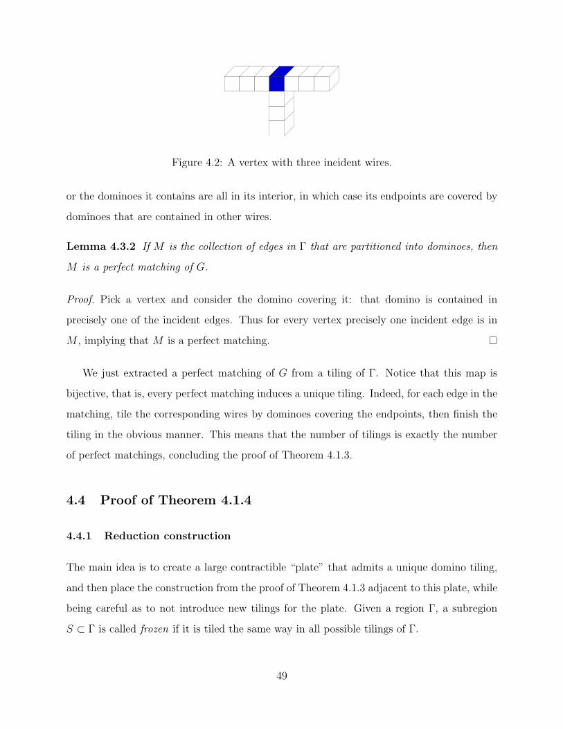
Figure 4.2: A vertex with three incident wires.

or the dominoes it contains are all in its interior, in which case its endpoints are covered by

dominoes that are contained in other wires.

Lemma 4.3.2 If M is the collection of edges in Γ that are partitioned into dominoes, then

M is a perfect matching of G.

Proof. Pick a vertex and consider the domino covering it: that domino is contained in

precisely one of the incident edges. Thus for every vertex precisely one incident edge is in

M , implying that M is a perfect matching.

We just extracted a perfect matching of G from a tiling of Γ. Notice that this map is

bijective, that is, every perfect matching induces a unique tiling. Indeed, for each edge in the

matching, tile the corresponding wires by dominoes covering the endpoints, then finish the

tiling in the obvious manner. This means that the number of tilings is exactly the number

of perfect matchings, concluding the proof of Theorem 4.1.3.

4.4 Proof of Theorem 4.1.4

4.4.1 Reduction construction

The main idea is to create a large contractible “plate” that admits a unique domino tiling,

and then place the construction from the proof of Theorem 4.1.3 adjacent to this plate, while

being careful as to not introduce new tilings for the plate. Given a region Γ, a subregion

S ⊂ Γ is called frozen if it is tiled the same way in all possible tilings of Γ.

49

We will call the z = k plane Layer k. The entire construction of Γ will lie in four layers,

from Layer −1 to Layer 2. When considering cubes on a layer, we will employ the usual

convention of referring to the +x, −x, +y, −y directions as right, left, above, and below.

When referring to an adjacent cube in a different layer, we will specify the layer specifically,

as to avoid confusion.

Let us start with a plate that lies in Layer 0, which is a region whose columns have

even lengths and are offset with each other, causing jagged borders. It is obvious that it

Figure 4.3: A plate with a unique tiling.

admits a unique tiling, which is shown in Figure 4.3. We will modify this plate carefully as

to introduce only local changes in the tilings while preserving the unique global tiling.

Suppose we are given a cubic bipartite graph G with bipartition A and B. We will place

the vertices in A on the left side of a plate, and vertices in B on the right side. Now we must

connect the corresponding vertices with wires. We can achieve the desired connections by

interchanging adjacent wires in steps. Indeed, think of the correspondence as a permutation

and write it as a product of transpositions. The resulting schematic is known as a wiring

diagram. These wires will, for the most part, stay in Layer 1. In between each pair of wires,

we will add a tension line. We then modify the region locally with a crossover X-gadget at

each location indicated in the wiring diagram.

As an example, we see the general picture in Figure 4.4. There is a big plate, with offset

columns causing jagged borders on the top and bottom of the region, indicated by the short

dashes. There are four vertices, each one with three wires coming out of it, indicated by the

50

Figure 4.4: Overview of the layout.

solid lines. The tension lines between the wires are indicated by the long dashed lines. The

red boxes are the X-gadgets.

The wire and the tension line are shown in Figure 4.5. The schematic is drawn in

(a) (b)

Figure 4.5: A wire (left) and a tension line (right).

Layer 0. The unique tiling of the frozen region in Layer 0 is shown: dominoes that are

entirely in this layer are drawn as 2× 1 rectangles in the plane. When a + (resp. −) sign is

present, it means the region includes the adjacent cube in Layer +1 (resp. −1).

Here we show half of a vertex V-gadget in Figure 4.6a. A single square in the schematic

denotes that the cube in Layer 0 is always tiled with a domino sticking out to Layer 1 or −1.

The symbol ± signifies that the adjacent cubes in both Layers ±1 are included. The blue

circle is the center of the V-gadget, and needs to satisfy positional parity as defined in the

proof of the previous theorem. Besides some isolated cubes, Layer 1 contains the wires.

Notice that there are three wires coming out of the center of the V-gadget. The third wire

that is not drawn completely in the figure should mirror the other wire in the obvious way,

51

(a) (b)

Figure 4.6: Half of a vertex V-gadget (left) and a hole H-gadget (right).

including the initialization of the tension line. The wires (sequences of +) extend towards

the right. Between each pair, we have a tension line (the sequence of jagged + and −).

Notice that we can easily make the V-gadgets taller as to have more separation between

the wires and tension lines exiting to the right. This will be used to align all these things

together correctly. We use the mirror image when putting the V-gadget on the right side of

the plate. Between pairs of V-gadgets, we also add tension lines running horizontally across

the entire plate.

To make the crossover X-gadget, we combine the hole H-gadget (Figure 4.6b) and the

splitter Y-gadget (Figure 4.7). We use the same schematic convention as above in these

figures. Here the symbol ⊕ denotes that there is a cube in Layer 1, but not in Layer 0.

Similarly, symbol signifies the inclusion of the cubes on Layers 1 and 2 (in addition to

Layer 0). First use the H-gadget to guide the lower wire to Layer −1, and use the Y-gadget

to merge and align them together. Then we reverse the process using a rotated copy of the

splitter, as to make the wires crossover each other. Finally, bring the wire back to Layer 1

with another H-gadget. This completes the construction of the crossover X-gadget.

It is clear that the X-gadget takes two wires on the left, separated by a tension line,

and outputs two wires on the right, again separated by a tension line. Notice that in the

construction of the X-gadget, we could make the output wires further away from each other,

52

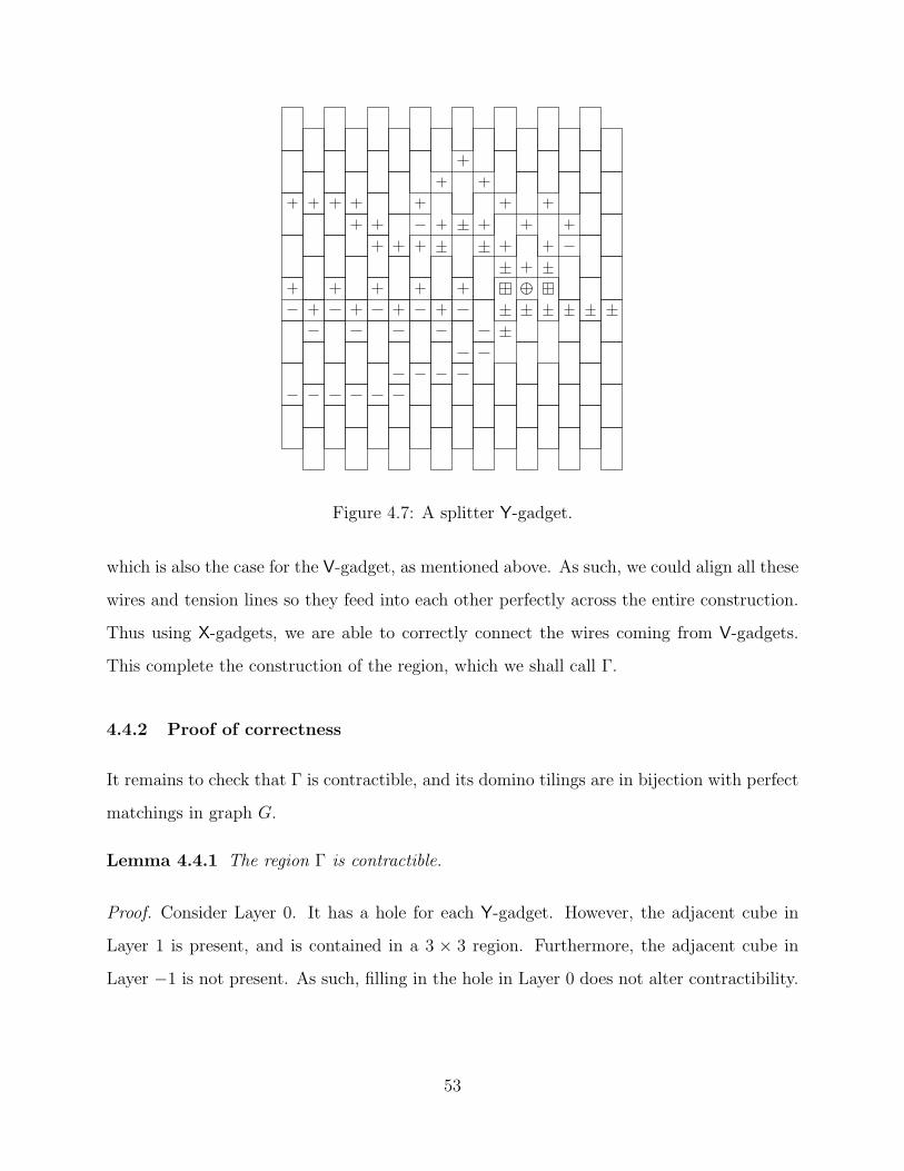
Figure 4.7: A splitter Y-gadget.

which is also the case for the V-gadget, as mentioned above. As such, we could align all these

wires and tension lines so they feed into each other perfectly across the entire construction.

Thus using X-gadgets, we are able to correctly connect the wires coming from V-gadgets.

This complete the construction of the region, which we shall call Γ.

4.4.2 Proof of correctness

It remains to check that Γ is contractible, and its domino tilings are in bijection with perfect

matchings in graph G.

Lemma 4.4.1 The region Γ is contractible.

Proof. Consider Layer 0. It has a hole for each Y-gadget. However, the adjacent cube in

Layer 1 is present, and is contained in a 3 × 3 region. Furthermore, the adjacent cube in

Layer −1 is not present. As such, filling in the hole in Layer 0 does not alter contractibility.

53

Now that there are no holes in Layer 0, we may deformation retract everything in other

layers to Layer 0, and then contract it to a point.

It remains to find a frozen subregion Γ′ ⊂ Γ such that Γ0 = Γ\Γ′ is a lattice drawing of

the given graph. Let us start with Γ′ = ∅ (thus Γ0 = Γ) and alter Γ′ inductively. A cube

in a region is isolated if it has precisely one neighbor (out of the six adjacent possibilities).

Notice that an isolated cube must be tiled by a domino covering its unique neighbor. We

will remove the isolated cubes of Γ0 by moving them from Γ0 to Γ′. We repeat this process

inductively until there are no more isolated cubes.

Lemma 4.4.2 At any step, Γ′ is a frozen subregion of Γ. When the process finishes, Γ0 is

a lattice drawing of the given graph.

Proof. It follows immediately by construction that Γ′ is frozen. The rest of this proof is

devoted to the second part of the lemma.

Let us perform another induction on the number of X-gadgets. For the base case, suppose

we did not have any X-gadgets. That is, we start with the boring cubic graph where disjoint

pairs of vertices are joined by three edges each.

Consider each V-gadget. After the first step, everything in Layers 0 and −1 on the two

left-most columns in Figure 4.6a are removed, leaving the wire in Layer 1. The tension lines

are all removed as well. It is clear that in the next step, the remaining horizontal domino

will also be removed, along with the domino above it.

Thus after two steps, what we are left with in Layer 0 is a collection of disconnected

plates, each of which has a wire across it horizontally in Layer 1. These wires protrude to

the left and right.

Each of these plates have jagged columns thanks to the initial boundary and the tension

lines. As such, in each step, the top- and bottom-most cubes are isolated, hence removed

with their neighbors, creating another jagged boundary. This process continues until all

cubes in Layer 0 are removed, including the ones adjacent to the wire in Layer 1. Note that

54

half of the cubes adjacent to said wire are removed from above, and the other from below.

Thus it is important that both sides were jagged, which is the motivation for introducing

the tension lines. We are left with the lattice drawing of the aforementioned contrived cubic

graph.

Now for the inductive step, suppose we add an extra X-gadget. We want to show that

the global situation is not altered, and that the local situation is what we wanted. Indeed,

the X-gadget consists of two H-gadgets and two Y-gadgets. Having analyzed the V-gadget,

one should be able to inspect the H-gadget construction in Figure 4.6b, and easily see that

after finitely many steps, we will be left with the wires in Layers ±1, plus the connecting

cube between them in Layer 0.

The Y-gadget is a bit more complicated, but can be carefully analyzed in the same

manner. Indeed, after the first step, all the cubes in Layer −1 are removed except for the

wire. Similarly, the Layers 1 and 2 cubes for are removed, so are all the cubes in Layer 1,

save the wire. As for Layer 0, we get a small island of six vertical dominoes in the middle,

and a giant plate with enough tension lines such that a similar inductive removal process as

above will remove it completely. Hence we are left with precisely the wires, thus completing

the proof of the lemma.

4.5 Proof of Theorem 4.1.1 and the first part of Theorem 4.1.5

4.5.1 Reduction construction

Here we reduce 1-in-3 SAT to a tiling problem. The reduction will be parsimonious, thus

proving both NP-completeness and #P-completeness.

Consider a sequence of cubes in the z = 0 plane, where two cubes are adjacent if and

only if they are consecutive elements in the sequence (this is called a wire in the proof of

Theorem 4.1.3). Consider the sequence as a region and duplicate it also in the z = 1 plane.

We now call a wire the union of these two copies. In a wire, a pair of adjacent cubes, one with

55

z = 0 and one with z = 1, is called a cube pair. In any tiling by slabs, each cube pair must

be covered by the same slab. If we translate the wire to the z = k and the z = k+ 1 planes,

we say the wire lives in the z = k biplane. Color the biplane χ(x, y, z) = x+ y (mod 2) in a

checkerboard fashion, ignoring the z-coordinate. We call the color of a cube (pair) its parity,

which can be even or odd. Similarly, we may rotate and consider wires living in x = k or

y = k biplanes. In those cases, the biplane coloring would ignore the x- or the y-coordinate,

respectively. Notice that a cube (x, y, z) ∈ Z3 might have different parities depending on the

biplane being considered. However, each cube pair lives in a unique biplane: thus the parity

of a cube pair is unambiguous. When we draw diagrams consisting of wires in each biplane,

we simply draw the two-dimensional regions used to form the wires.

The variable V-gadget, shown in Figure 4.8, is made by removing two diagonal cubes of

a 2× 2× 2 region, and then attaching six wires. Notice that the wires come in pairs, and

z

yx

+y

−y

−z

+z

+x

−x

Figure 4.8: A variable V-gadget, with six wires coming out of it.

each pair lives in a biplane. We label the wires with their initial coordinate directions. Each

wire has an endpoint in the V-gadget, called the variable endpoint ; the other one is called

the free endpoint. We now describe where to place the V-gadgets and how to join these free

endpoints together.

56

Suppose we are given a 3-SAT expression C = C1, . . . , Ct on the variable set X =

v1, v2, . . . , vn, where each clause Ci = (ci1, ci2, ci3) consists of three literals, each either a

variable vk or a negation vk, for some k ∈ [n] = 1, . . . , n. We now construct a region Γ.

If cij is vk or its negation vk, place a V-gadget at (10k, 10(3i + j), 0). That is, the wires

live in the x = 10k, y = 10(3i+ j), and z = 0 biplanes, respectively. Moreover, the variable

endpoint of each wire has odd parity with respect to the coloring of the biplane in which the

wire lives.

Consider the x = 10k plane for each k ∈ [n], which is drawn schematically in Figure 4.9.

Notice that all the ±z wires corresponding to the variable vk are on this biplane. For each

+

v−

+

v−

+ +

v v− −

y

z

Figure 4.9: Synchronization of variables: This is a diagram in some x = 10k (bi)plane. The

squares represent the V-gadgets and the lines represent the wires.

V-gadget, we will bend the +z wire to the left and down as shown. We link up the first wire

with the last, and also the remaining adjacent pairs.

Figure 4.10 shows a clause C-gadget, which is simply a joining of three wires. The parity

Figure 4.10: A clause C-gadget, where three wires meet.

of the gadget is the parity of the blue cube pair at the center where the three wires meet.

Now let us work in the z = 0 biplane, schematically shown in Figure 4.11. For each

57

++

+

−−

−v

x

y1

6v3

odd

v

even

Figure 4.11: Diagram in the z = 0 (bi)plane. The circles, where the lines meet, indicate the

C-gadgets, which are at two different parities.

clause, there are three corresponding V-gadgets. From each V-gadget, take the +y (resp. −y)

wire if the corresponding variable appears in the clause unnegated (resp. negated). Extend

these three wires to x = 10(n + 1) and join them together at a C-gadget with even parity.

Similarly, extend the three remaining ±y wires to x = −10 and join together at a C-gadget

with odd parity. We call these the even and odd C-gadgets corresponding to each clause,

respectively.

Finally, for each V-gadget, let us join the remaining +x wire and the −x wire together

to form a loop.

Lemma 4.5.1 The wires can be joined together such that no cubes are adjacent unless they

are in fact adjacent cubes from a single wire.

Proof. As the V-gadgets are sufficiently spaced out, it is very obvious that we can make the

wires avoid each other, besides when they meet at the V- and C-gadgets.

This finishes the construction.

4.5.2 Proof of correctness

Fix a region Γ constructed above from a 3-SAT expression C. It remains to show that the

tilings of Γ and the 1-in-3 satisfying assignments of C are in bijective correspondence.

58

First, consider a tiling of Γ. We say that the phase of an endpoint of a wire is positive if

the wire contains the tile that covers that endpoint, and negative otherwise.

Lemma 4.5.2 A wire of even length has the same phase at both endpoints, while a wire of

odd length has opposite phases at its two endpoints.

Proof. As in the proof of Theorem 4.1.3, the slabs must line up along the length of the wire,

since the various wires do not intersect or come near each other (except at the endpoints).

The following is immediate by observing the way slabs can come together to tile the

V-gadget:

Lemma 4.5.3 There are two ways to tile each V-gadget locally. In either tiling, the three

+ wires have the same phase at their variable endpoints, and the three − wires have the

opposite phase at their variable endpoints as the + wires.

Let the phase of the V-gadget be the common phase of the + wires at their variable

endpoints.

Lemma 4.5.4 The V-gadgets corresponding to vk (or its negation vk) all have the same

phase.

Proof. Consider two adjacent V-gadgets in the construction shown in Figure 4.9. Sup-

pose the gadget on the left has positive phase (the opposite situation is similar). Then

by Lemma 4.5.3, its −z wire has negative phase at the variable end. This wire is linked with

the +z wire of the gadget on the right. Since both endpoints have odd parity, the wire has

odd length, thus by Lemma 4.5.2, the variable endpoint of the +z wire of the gadget on the

right (hence the gadget) has positive phase.

This allows us to assign a truth value to the variable vk:

Lemma 4.5.5 Let the boolean assignment of vk be the common phase of the V-gadgets

corresponding to vk. This defines a 1-in-3 satisfying assignment.

59

Proof. Fix a clause (c1, c2, c3) and consider the corresponding even C-gadget. There are three

wires connecting the corresponding V-gadgets to the center of the C-gadget. The variable

endpoints of the wires have odd parity, and the free endpoints are all at the center of the

C-gadget, which has even parity. As such, the wires have even lengths; thus by Lemma 4.5.2,

each wire has the same phase on both its endpoints.

The center of the C-gadget is tiled by some slab, which is contained in precisely one of

its three wires. Without loss of generality, suppose only the wire corresponding to c1 is of

positive phase (at both of its endpoints). Recall that the phase of a V-gadget is the phase

of its + wires at their variable endpoints. If ci = vk is an unnegated variable, then the +y

wire was used, and thus vk (and hence ci) is positive if and only if i = 1. On the other hand,

if ci = vk is a negated variable, then the −y wire was used. Thus vk is negative if and only

if i = 1, but then ci is again positive if and only if i = 1.

This shows that the assignment is indeed 1-in-3 satisfying. We thus have a map from the

tilings of Γ to the satisfying assignments of C.

For the inverse, suppose we have a 1-in-3 satisfying assignment. Simply tile each V-gadget

according to the assignment in the obvious way. It only remain to tile the wires. However,

by construction, once we choose the phase of a V-gadget, the tiling of all six wires emanating

from that region is forced.

The ±z wires fit together because the phases of the V-gadgets are consistently assigned,

in accordance to the truth value of the variable in the given satisfying assignment.

Recall that for each V-gadget, its +x and −x wires form a loop. Since the two endpoints

both have odd parity, the length of the wire is odd. By Lemma 4.5.2, the two endpoints

have opposite phases in a tiling, which is precisely what the V-gadget would produce as in

Lemma 4.5.3.

It is obvious that the ±y wires fill up the even C-gadgets perfectly because the boolean

assignment was 1-in-3 satisfying. For the odd C-gadgets, notice that since we take the leftover

wires, precisely one of the three is negative at its variable endpoint. However, since we join

60

them at a cube pair with odd parity, the wires are of odd lengths, thus precisely one of the

three is positive on the free endpoint at the C-gadget, as needed.

This establishes the desired bijective correspondence, and implies that the construction

is indeed a parsimonious reduction from 1-in-3 SAT to the slab tiling problem, concluding

the proof of Theorem 4.1.1. Note that this also implies that the associated counting problem

is #P-complete, yielding the first part of Theorem 4.1.5; in the next section we prove a

stronger result.

4.6 Proof of Theorem 4.1.2 and the second part of Theorem 4.1.5

4.6.1 Reduction construction

Given a region Γ0 as constructed from the previous section, we will enlarge it to a contractible

region Γ ⊃ Γ0, such that Γ′ = Γ\Γ0 is a frozen subregion of Γ.

z

y

x

z

yx

Figure 4.12: A variable V-gadget, shown in two perspectives.

First we modify the variable V-gadget. The following description is relative to a V-

gadget placed at (0, 0, 0). We must make these adjustments to each V-gadget used. Recall

that in the proof of Theorem 4.1.1, each +z wire was bent as in Figure 4.9. Let us make

this precise by making it bend towards the −y direction when it hits z = 3, and bend

towards −z when it hits y = −5 (see Figure 4.12). We define a region X, shown in Fig-

61

z

xy

1 2 3

4 56

(a) Region X.

z

yx

1

1

1

1

1

22

2

2

2

33

4

(b) Region Y .

Figure 4.13: Regions used to modify the V-gadget.

ure 4.13a, that will fill the hole this loop makes. Indeed, let X = −1 × [−5, 0] × [0, 3] ∪

(0,−1, 0), (0,−1, 1)\(−1, 0, 0), (−1, 0, 1). The unique tiling is indicated in the figure;

the labels will be used in the proof of Lemma 4.6.2. Similarly, the ±x wires are linked

together to form a loop. Let us bend them towards the +z direction when they hit 4 and

−3, respectively, and bend towards each other when they hit z = 5. Define a region that

will fill this hole, shown in Figure 4.13b: Take

[−3, 4]× 2 × [0, 5],

add the following six cubes

(−4, 2, 0), (−4, 2, 1), (1, 3, 0), (2, 3, 0), (1, 1, 1), (2, 1, 1),

and remove these two cubes

(0, 2, 0), (0, 2, 1).

Call this region Y . Note that the slab labeled 4 in the figure extends behind and is hid-

den from view. We will add regions X and Y to the V-gadget. This makes the V-gadget

contractible.

Let Z = [−10, 10n+ 11]× [0, 30(t+ 1) + 1]× −1 ⊂ Z3, where n and t are the number

of variables and clauses, respectively. We then modify Z with a hole H-gadget around each

V-gadget to allow its ±z wires to pass through. Indeed, Figure 4.14 shows the construction

62

zx

y

1 1

Figure 4.14: A hole H-gadget.

in the z = −1 plane viewed from below. The surrounding slabs on the boundary match that

of the unique tiling of Z. The two cube pairs missing allow the ±z wires to pass through

(spaced out according to the precise construction of the V-gadget in Figure 4.12). The cube

pairs in z = −2 plane are necessarily tiled with its unique neighbor in the z = −1 plane.

Let Xk = 10k− 1× [0, 30(t+ 1) + 1]× [−9,−2] for each k ∈ [n]. Here we assume that the

linking of the ±z wires (see Figure 4.9) are done at z-coordinates, say, −5 and −7, which

are in [−9,−2]. Let Γ′ be the disjoint union of the X and Y for each V-gadget, the region

Z, and the Xk for each k. This finishes the construction.

4.6.2 Proof of correctness

It remains to check that that the construction works. The following two lemmas easily imply

the result.

Lemma 4.6.1 The region Γ constructed above is contractible.

Proof. Notice that there are no holes in the z = −1 plane. In z < −1, we may deformation

retract the wires onto the Xk plates, and then deformation retract these plates onto the

z = −1 plane.

We now check that the modified V-gadget is contractible. The center of an original

V-gadget was an example of a non-contractible region shown in Figure 4.1. Indeed, the

interior will leave a point hole in the middle; however, it is filled by the slab labeled 4 in

63

Figure 4.13b. The loop formed by the +z wire bending down is filled by X, while the loop

formed by joining the ±x wires is filled by Y . Moreover, the ±y wires are all lying along Z so

we may deformation retract everything to the z = −1 plane. We omit the (easy) details.

Lemma 4.6.2 The subregion Γ′ ⊂ Γ is frozen.

Proof. Consider a cube c ∈ Γ. If it forms a 3× 1× 1 region with a cube pair, then no slab

containing this cube may contain its neighbor that is part of the cube pair. Not counting

such cube pairs, if c only has two neighbors left, then c must be tiled by a slab covering

both these neighbors. If this happens, we call c isolated and say that it forces the unique

slab containing c. Just like in the proof of Theorem 4.1.4, we may inductively remove these

forced slabs, which are obviously frozen.

Consider region Xk. Notice that the cube at the corner (10k− 1, 1,−9) is isolated. After

removing the slab forced by it, we may consider the new corner next to it at (10k−1, 3,−9).

Inductively, we may remove the cubes with z = −9 or −8. Now when looking at z = −7,

we may run into cubes that neighbor ±z wires. However, these wires are made of cube pairs

that form 3×1×1 regions with the cubes in question. As such, we may continue the removal

process unhindered. It is clear that in this manner, we may remove all cubes from Xk.

Similarly, we remove most slabs from Z, starting from the boundary and working our

way in. The ones sticking down out of the z = −1 plane can also be removed, leaving us

with precisely two slabs around the hole for the −z wire from the H-gadget (labeled with 1 in

Figure 4.14). As for each V-gadget, we remove all the cubes from X and Y . In Figure 4.13,

the forced slabs are labeled with a sample removal order, where each number is positioned on

the isolated cube used at each step. Finally, we may remove the leftover slabs from Z.

Now, given a 1-in-3 SAT expression C, we may take a region Γ0 constructed in the

proof of Theorem 4.1.1 and enlarge it to a contractible region Γ as described above. Since

Γ′ = Γ\Γ0 is frozen, Γ is tileable if and only if Γ0 is tileable. These are tileable if and only

if C is 1-in-3 satisfiable, thus Theorem 4.1.2 is proved. Moreover, since both reductions are

parsimonious, we conclude the second counting result in Theorem 4.1.5 as well.

64

4.7 Generalized dominoes in higher dimensions

Let Ddr ⊂ Zd be a 2 × . . . × 2 × 1 × . . . × 1 region with r number of 2’s and d − r number

of 1’s. We call this a generalized domino in d dimensions of rank r. Call the r coordinate

directions that are 2 cubes wide fat. Previously we were concerned with tiling by dominoes

D31 and slabs D3

2 in three dimensions.

Theorem 4.7.1 For 2 ≤ r < d, tiling (contractible) d-dimensional regions with Ddr is NP-

complete. Similarly, for 1 ≤ r < d and d ≥ 3, tiling (contractible) d-dimensional regions

with Ddr is #P-complete.

Note that in other cases of r and d, these problems are in P (see next section).

Proof. We reduce specific tiling problems in Z3 to higher dimensions. Let us first prove the

statements without the contractibility constraint.

Suppose 2 ≤ r < d. Let Γ ⊂ Z3 be a region as afforded by the proof of Theorem 4.1.1.

Let Γ′ = Γ×0, 1r−2×0d−r−1, that is, (x1, . . . , xd) ∈ Zd : (x1, x2, x3) ∈ Γ, x4, . . . , xr+1 ∈

0, 1, xr+2 = . . . = xd = 0. Consider a tiling of Γ′ by Ddr . Notice that there are no 2×2×2

subregion in Γ, thus each tile must be oriented with two of its fat directions in the first three

coordinates, the remaining r − 2 fat directions in the next r − 2 coordinates. This means

that any Ddr -tiling of Γ′ induces a D3

2-tiling of Γ. It is easy to see that this correspondence

is actually a bijection, finishing the proof of NP-completeness, and also #P-completeness

when r ≥ 2.

The case of r = 1 is straightforward. Take Γ from the proof of Theorem 4.1.3. Define

Γ′ = Γ× 0d−3, and follow the argument above.

To prove the result for contractible regions, proceed in the same manner, and take the

regions constructed in the proof of the corresponding theorems. For 2 ≤ r < d, take the

region Γ from the proof of Theorem 4.1.2, and define Γ′ in the same way as above. Notice,

however, that the above strategy does not yield a reduction from D32-tilings to Dd

r -tilings

in general. Indeed, we used the fact that the specific Γ ⊂ Z3 did not contain 2 × 2 × 2

65

subregions, which is no longer the case. The outlined argument actually still works, but

more care must be taken. A tile might now be oriented with three of its fat directions in

the first three coordinates. This means a Ddr -tiling of Γ′ will, a priori, induce a tiling of Γ

with slabs and the [2× 2× 2] cube. However, in the proof of Theorem 4.1.2, we see that no

tilings of Γ by slabs contain a 2× 2× 2 subregion tiled by two slabs. As such, all Ddr tiles in

Γ′ are still constrained to be oriented as before, with precisely two fat directions in the first

three coordinates. This implies the result in this case.

The same approach works for the r = 1 case as well. Take Γ as in the proof of Theo-

rem 4.1.4, and define Γ′ as above. Now notice that in any tiling of Γ, there is no 2 × 2 × 1

subregion of Γ that is tiled by two dominoes, which proves the result.

4.8 Final remarks and open problems

4.8.1

Historically, the tiling problems played a crucial role in the developments of modern theo-

retical computer science. The tileability of the whole plane with a set of tiles was shown

to be undecidable [Ber66, Rob71]. A version of the finite tileability problem was stated

to be NP-complete in Levin’s original paper [Lev73], where he (independently) defined NP-

completeness. Finally, Theorem 4.1.3 is one of the first few applications of #P-completeness,

developed by Valiant [Val79b].

4.8.2

In the context of statistical physics, the domino tiling problem is called the dimer problem,

and has a long history. The classical results of Fisher [Fis61] and Kasteleyn [Kas61] express

the number of domino tilings of finite regions in the plane as a certain Pfaffian, equal to

a square root of a determinant. A closely related monomer-dimer model is #P-complete

already in the plane [Jer87] (see also [Vad01]). Let us mention that both models can be

66

polynomially approximated (see [JSV04, KRS96]). We refer to [Tho06] for graph-theoretic

reasons precluding the Pfaffian method in higher dimensions, and to [DG00, HK81] (see

also [HN04]) for the general hardness results on graph homomorphisms, a concept generalizing

perfect matchings.

4.8.3

In the general tileability problem, a set T of tiles is fixed, and one considers tilings with

parallel translations of copies of tiles T ∈ T. For a single tile T , the tileability problem is a

special case, where T consists of all reflections and rotations of T . Let us briefly elaborate

on the state of art of these tiling problems as they pertain to our results.

In the plane, when |T| = 1, i.e., when translates of a single tile are used, the tileability

problem is linear in the area. However, already for T = 2 × 1, 1 × 3, the tileability is

NP-complete [BNRR95]. It is not known whether the corresponding counting problem is

#P-complete. The smallest set T for which #P-completeness is known is the set of four

rotations of the L-tromino and a [2× 2] square [MR01].

For simply connected regions in the plane, we recently found a set of 23 Wang tiles, which

they showed to be NP-complete and #P-complete (see Chapter 2). This construction can

be further decreased to 15 tiles (Lemma 3.1.1), and we conjecture that only three rectangles

suffices (see Subsection 2.7.5). In contrast to the decision problem, it is still unclear how

much the simple connectivity of regions helps counting the number of tilings, other than

making the reductions harder and more technical.

4.8.4

In [Val79a], Valiant’s goal is to show the hardness of the number of perfect matchings of

grid graphs, defined as subgraphs (of the unit distance graph) of Z3. This is slightly weaker

than the hardness of domino tilings of 3-dim regions, since the latter problem corresponds to

induced subgraphs of Z3. However, Valiant’s proof can be slightly modified, from subgraphs

67

of [2× n× n] to induced subgraphs of [3× n× n], to achieve the same goal. The proof we

present in Section 4.3 is in fact a variation of the argument in [Val79a].

4.8.5

For tiling in three dimensions, we consider the domino and the slab. Here each tile has three

distinct orientations. If we only allow two out of the three orientations in either case, each

problem becomes equivalent to the ordinary domino tiling problem in two dimensions, and

hence is in P. Of course, two orientations suffices for the tromino tile I3 = [3 × 1 × 1] (or

the [3 × 3 × 1] tile) to guarantee NP-completeness, since we have NP-completeness for the

[3× 1] tile.

Note that the augmentation approach, mentioned in the introduction, allows us to show

the NP-completeness of the tileability problem with I3 of contractible regions in R3. To see

this, start with a flat region and color the holes in a checkerboard fashion. Now fill each

unit cube with an up or down vertical tromino, depending on the color (see Figure 4.15).

The contractible region thus obtained is tileable with I3 if and only if the starting region is

tileable by [3× 1].

Figure 4.15: A construction of contractible 3-dim regions for tromino tilings.

4.8.6

The conditions in Theorem 4.7.1 are best possible. Indeed, if r = 0 or r = d, we are tiling

with cubes of side length 1 or 2, respectively, both of which are linear in the volume. The

68

only remaining cases are the decision problem with Dd1, and the counting problem of ordinary

dominoes in dimension d = 2, both of which are in P (see e.g. [LP09]).

4.8.7

The idea of graph embedding into a grid is quite standard. In this context of domino tilings

it was used in [DKLM10, Val79a], and for other small sets of tiles in [BNRR95, MR01] and

Chapter 2. Of course, the technical details are somewhat different in each case.

4.8.8

It would be interesting to see if Theorem 4.1.4 holds for contractible regions inside a [2×n×n]

brick, as they have a rather simple geometric structure. Our proof gives only a width 4

bound, but we believe that a width 3 modification can be made without difficulty. We

should mention that for every fixed c, the counting problem is polynomial for regions inside

a [c× c× n] brick.

4.8.9

In the plane, there are several other generalizations of domino tilings. Notably, ribbon tilings

was introduced and studied (see [Pak03]). Another interesting set of generalized dominoes

Tn = 2k × 2n−k, 0 ≤ k ≤ n was studied in [Kor04]. Both sets satisfy the local move

property: every two tilings of a s.c. region Γ can be obtained by a sequence of flips, each

involving a fixed number of tiles (2 in both cases, see [Pak03]). For the (usual) domino tilings

this is a classical property going back to Kasteleyn and famously proved by Thurston via

the height functions [Thu90].

Of course, for the domino tilings of general regions there is no local move property, as large

cycles can involve an unboundedly many tiles. However, for contractible regions, one would

naturally assume that domino tilings and slab tilings are connected by flips corresponding to

69

different tilings of [2× 2× 2]. This is, in fact, false. As an early prequel to the constructions

in the proofs of theorems 4.1.2 and 4.1.4, we state the following easy result.

Proposition 4.8.1 Domino tilings of contractible regions in R3 does not have the local move

property. The same result holds for slab tilings.

The proof is apparent from Figure 4.16 (cf. Figure 4.15). In the first case, the middle

dominoes alternate between up and down. In the second case, slabs are all vertical, with the

middle slabs all one layer below.

Figure 4.16: Cross sections of large regions in R3 with exactly two tilings, by dominoes and

by slabs, respectively.

70

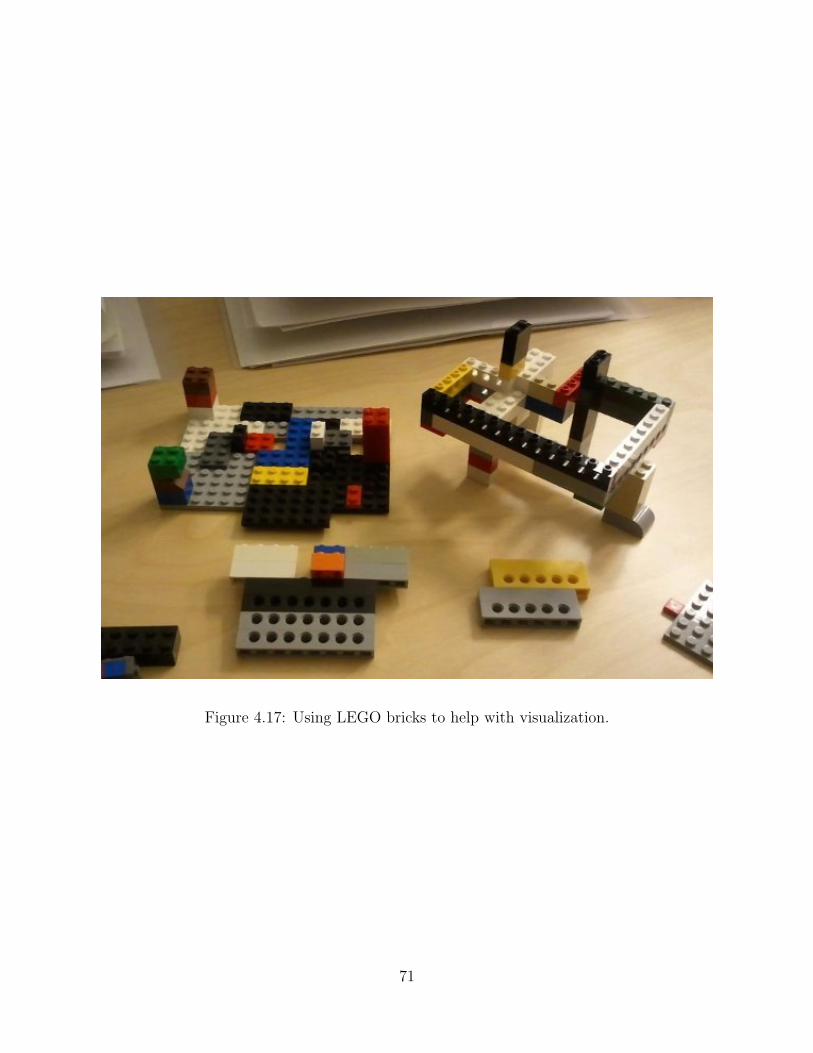
Figure 4.17: Using LEGO bricks to help with visualization.

71

CHAPTER 5

Rectangular tileability and complementary tileability

are undecidable

Does a given set of polyominoes tile some rectangle? We show that this problem is unde-

cidable. In a different direction, we also consider tiling a cofinite subset of the plane. The

tileability is undecidable for many variants of this problem. However, we present an algo-

rithm for testing whether the complement of a finite region is tileable by a set of rectangles.

5.1 Introduction

Tileability on the plane has been a subject of much study [GS87]. A lot of focus was in tilings

on the square grid by polyominoes [Gol65], including establishing NP-completeness [Lew78,

MR01] and finding efficient algorithms when possible [KK92, Rem05]. Aperiodicity in tilings

of the entire plane has also been well studied [Moz97, Pen74], with connections to ergodic

theory [Rad99, CR98] and quasicrystals [DS99]. Recently, a single (disconnected) tile that

exhibits aperiodic behavior was found [ST11], partially settling a famous open problem.

Can the plane be tiled using translated copies of a given set of polyomino tiles? Berger

showed that this decision problem is undecidable [Ber66], meaning that there is no general

algorithm that can always answer this question from the input. This implies that there

exists aperiodic tilesets, i.e., tiles that can only tile the plane without translational symmetry.

Indeed, Berger provided an aperiodic tileset of 20426 tiles, and Robinson reduces this number

to 6 if rotations and reflections are allowed in addition to translations [Rob71]. This disproves

a conjecture of Wang (see Subsection 5.7.4).

72

To have aperiodicity and undecidability, clearly the complexity of tiles and tilings must

increase without bound. The following result shows that one can encode this complexity in

a single tile alone.1

Theorem 5.1.1 (Complementary Tileability) There is a tileset T such that it is undecidable

whether the complement of a finite input region Γ is tileable by T.

Instead of tiling the entire plane or a cofinite subset, we also consider tiling finite regions.

If a rectangle is tileable, then of course the plane is tileable. Thus the following is a variation

of the result above.

Theorem 5.1.2 (Rectangular Tileability) It is undecidable whether a given tileset T can

tile some rectangle.

This should be contrasted with tiling a given rectangle by a fixed tileset:

Theorem 5.1.3 ([LMP05]) Tileability of an [n × m] rectangle by a fixed tileset can be

determined in time O(log n+ logm).

We discuss this connection and some curious consequences of Theorem 5.1.2 in Subsec-

tion 5.7.2. It is worth noting that if we are given a finite region to tile as opposed to the

entire plane, the problem is decidable simply with exhaustive search (see Subsection 5.7.1

for results in this finite setting). However, although the region to be tiled in Rectan-

gular Tileability is finite, the problem is (potentially) undecidable as the finite region

is unspecified. That is, we are tiling a finite object from an infinite collection. Indeed,

Theorem 5.1.2 shows that Rectangular Tileability is undecidable. We prove this in

Section 5.3, where we moreover show that the problem remains undecidable when the size

|T| of the tileset is fixed. Also, as a corollary, we see that tileability of a unit square by

finitely many similar copies of tiles (where rotations, reflections, and dilations are allowed in

addition to translations) is also undecidable.

1We require that this tile be used precisely once. To that end, we consider it as an input and tile itscomplement by a fixed tileset.

73

In Section 5.6, we prove undecidability for Augmentability, where we are to augment

a finite simply connected region Γ by tiles so that the union is tileable. Any augmentable

region Γ by the (horizontal and vertical) dominoes must necessarily be balanced, i.e., has

the same number of black and white squares when the plane is colored as a checkerboard.

Korn showed that this is not sufficient, and also proved that Γ is augmentable if it is row-

convex, i.e., each horizontal row forms a single contiguous region [Kor04, §11]. This should

be compared with Theorem 5.1.4 below.

Usually once a result is established for a decision problem with several inputs, one may

consider fixing some of these inputs and aim to obtain the same conclusion. To that end,

we fix the tileset and instead let the region vary as the input of Tileability. However,

decidability makes sense only if the input is finite, yet the region is infinite. As such,

in Section 5.4, we consider some variations of tiling cofinite regions. Though most of these

problems are undecidable, in the positive direction, we provide an algorithm for Tileability

of cofinite regions by arbitrary sets of rectangular tiles.

Theorem 5.1.4 It is decidable whether the complement of a given finite region Γ is tileable

by a given tileset T consisting only of rectangles.

In contrast, we show in Section 5.5 that Tileability of indented quadrants by rectangles

is undecidable.

5.2 Basic definitions

We call a subset of Z2 a region. By identifying Z2 as a union of closed unit squares in R2

centered at the integer lattice points, a region takes on a geometric shape in the obvious

manner. We freely switch between viewpoints when convenient.2 We say a finite region is

an (polyomino) tile if its shape is simply connected (s.c.). A finite collection of tiles is called

a tileset. Note that Z2 acts naturally on a tile by translation. Given a region Γ and a tileset

2For example, finite and disjoint refer to regions as subsets of Z2, so the shapes of disjoint regions (e.g.,tiles in a tiling) may intersect on their boundaries, but simply connected refers to the shapes of regions.

74

T, a T-tiling is a partition of Γ into translated copies of tiles in T. A region is T-tileable

if it admits a T-tiling. When the tileset T is understood, we may suppress the prefix for

notational convenience.

The boundary of (the shape of) a tile consists of unit-length horizontal and vertical edges.

A (generalized) Wang tile is a tile whose edges are labeled with symbols that are referred

to as colors. When tiling with Wang tiles, incident edges must be the same color. When a

Wang tile is a single square, it is also called a Wang square.3

Consider the following decision problem:

Tileability

Instance: A tileset T and a region Γ.

Decide: Does Γ admit a T-tiling?

Berger proved that Tileability for Wang squares is undecidable when Γ = Z2 is the

whole plane [Ber66]. By straight-forward reductions (see Lemma 2.3.1), most problems

involving tileability of polyominoes, generalized Wang tiles, and Wang squares are equivalent.

In this chapter we will consider a few other tileability problems that are undecidable. We will

usually state theorems for polyominoes, but prove them (first) for Wang tiles, then appeal

to the reductions in the appendix.

5.3 Rectangular tileability

Here we consider the decision problem Rectangular Tileability, where the input is a

tileset and the region to be tiled is unspecified.

Rectangular Tileability

Instance: A tileset T.

Decide: Does there exist some rectangle that is tileable by T?

3In the literature, a square Wang tile is usually simply called a Wang tile and sometimes called a dominodespite being a single square.

75

By an alphabet Σ we mean a set of symbols, whose elements could be juxtaposed to form

words. Let Σ∗ denote the set of all finite words in the alphabet Σ. The Post Correspon-

dence Problem is a well-known undecidable decision problem:

PCP

Instance: An alphabet Σ, positive integer n, and words jt, kt ∈ Σ∗ for t ∈ [n].

Decide: Does there exist a positive integer d and ei ∈ [n] for i ∈ [d], such that

the concatenated words je1je2 . . . jedand ke1ke2 . . . ked

are the same?

Theorem 5.3.1 ([Pos46]) PCP is undecidable.

Given a PCP instance I, we will construct a tileset T such that T tiles some rectangle

if and only if I admits a solution, and thus proving Theorem 5.1.2.

Lemma 5.3.2 Given a PCP instance I, there is a computable4 tileset W of generalized

Wang tiles such that W tiles a white rectangle if and only if I admits a solution.

Proof. For each jt = x1x2 . . . xr ∈ Σ∗, create a 1 × r tile Jt whose top boundary edges

are all colored U , the bottom color sequence is (x1, t), x2, . . . , xr, and the vertical sides are

colored V . Similarly for kt = y1y2 . . . ys ∈ Σ∗, create a 1 × s tile Kt whose top boundary is

(y1, t), y2, . . . , ys, the bottom colored D, and the vertical sides are colored V (Figure 5.1).

For each x ∈ Σ and t ∈ [n], create the following six transmitter tiles in Figure 5.2. Finally,

add in the border tiles in Figure 5.3, which are the only ones with white (unlabeled) colors.

This finishes the construction of the tileset W.

If I has a solution e1, . . . , ed, we first put Je1 , Je2 , . . . , Jedin a row on top, Ke1 ,Ke2 , . . . ,Ked

in a row on the bottom. If we view the color (x, t) as x, then the bottom of the top row

and the top of the bottom row have the same color sequence. The transmitter tiles allow

“shifting” the tag t to the left or right one step at a time until they match up as well. We

4The main proof technique of undecidability is by reducing a known undecidable problem to the currentproblem. This transformation must be done in a computable manner, i.e., by a deterministic algorithm.Thus computable means that the existence of the object in question can be substantiated by an explicitconstruction.

76

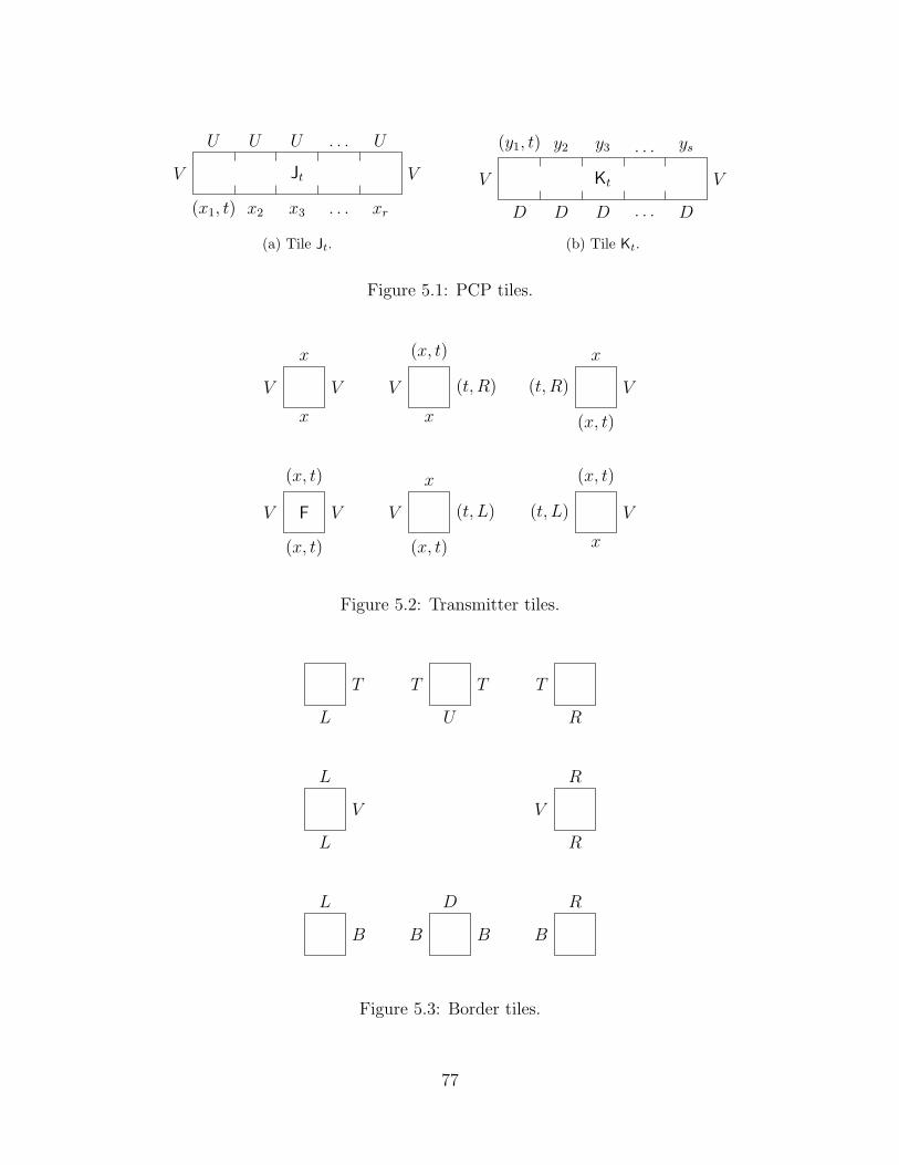
Jt

(x1, t)

U U U

x2 x3 . . .

. . .

xr

U

V V

(a) Tile Jt.

Kt

(y1, t)

D D D

y2 y3

. . .

. . . ys

D

V V

(b) Tile Kt.

Figure 5.1: PCP tiles.

V

x

x

V V

(x, t)

x

(t, R) (t, R)

x

(x, t)

V

V

(x, t)

(x, t)

VF V

x

(x, t)

(t, L) (t, L)

(x, t)

x

V

Figure 5.2: Transmitter tiles.

L

T T

U

T T

R

L

L

V V

R

R

L

B B

D

B B

R

Figure 5.3: Border tiles.

77

thus have a rectangle with the top and bottom colored U and D, respectively, while the

vertical sides are colored V . Notice that the border tiles can tile a rectangular border of any

size, whose outside boundary is white, and the inside colors match exactly what we have.

Conversely, suppose W tiles a white rectangle. Consider the smallest white rectangle it

can tile. The border tiles occur only on the boundary. Indeed, if there is any border tile in

the interior, by construction, it must form a white rectangular frame with filled interior, a

contradiction to the minimality. Now remove the border tiles on the boundary, the top (resp.

bottom) row must be a sequence of Jt (resp. Kt) tiles. Let e1, . . . , ed be the indices of the

top sequence. By construction of the transmitter tiles, the bottom sequence share the same

indices. Furthermore, viewing the color (x, t) as x, the color sequences are the same. This

means that the concatenated words coincide, and we indeed extracted a solution to I.

Corollary 5.3.3 Given a PCP instance I, there is a computable tileset T of polyominoes

such that T tiles a rectangle if and only if I admits a solution.

Proof. Take the set W of generalized Wang tiles afforded by Lemma 5.3.2, and transform it

to a set T of polyomino tiles using Lemma 2.3.1 with a minor change. In the construction,

we will replace the color white by a straight boundary, including the omission of the corner

zig-zags.

If I admits a solution, then there is a tiling of a white rectangle by W. Replace each

Wang tile by its corresponding polyomino in T. By construction, they fit together to form

a tiling of a rectangle by T.

Conversely, suppose T tiles some rectangle. Consider the smallest rectangle tileable by T

and fix one such tiling. Note that the only tiles that can touch the boundary of the rectangle

are the border tiles (i.e., those tiles in T that correspond to the border tiles in W), lest

there be small holes that cannot be filled. Conversely, the border tiles cannot occur in the

interior by minimality, since they always form rectangular frames. We have replicated the

exact same situation as in the proof of Lemma 5.3.2, allowing us to extract a minimal Wang

tiling of a white rectangle, and thus a solution to I, as desired.

78

This concludes the proof of Theorem 5.1.2. Moreover, we can allow the pieces to be

rotated, reflected, or even dilated.

Corollary 5.3.4 It is undecidable whether a tileset T can tile a unit square with finitely5

many similar copies of its tiles.

Proof. We claim that the specific tiles T in the proof of Corollary 5.3.3 tile a rectangle by

translation alone if and only if it admits a similar tiling of the unit square.

Suppose T tiles some [a × b] rectangle by translation. By repeating the rectangle ab

times, we have a tiling of an [ab× ab] square. Dilating, we obtain a similar tiling of the unit

square.

Conversely, suppose T admits a similar tiling of the unit square. Let S be the union of all

tiles with the minimum scaling factor. All the corner zig-zag of tiles in S must be matched

by other tiles of the same scaling factor. As such, all tiles that touch the boundary of S must

be border tiles. In the proof of Lemma 2.3.1, we note that the interlocking corner zig-zags

force all tiles to have the same orientation. This works even when we removed the corner

zig-zags for the white edges. In this case, each border tile must be part of a rectangular frame

with all its border tiles in the same orientation. Since there are finitely many rectangular

frames, there exists one without border tiles within. This rectangular frame is fully tiled in

its interior by tiles at this minimum scaling factor. Indeed, if there were any gaps, that would

be a boundary of S, a contradiction. Finally, note that all tiles in this rectangular region

has the same orientation. Thus T tile some rectangle by translation alone, as desired.

Theorem 5.1.2 remains true even if the number of tiles is bounded.

Theorem 5.3.5 Rectangular Tileability with 19 tiles is undecidable.6

5If infinitely many similar copies are allowed, any tileset can tile a unit square greedily in a manner akinto that of an Apollonian gasket.

6Of course, the number of tiles can be incremented by splitting a tile in such a way that the pieces mustreassemble to form the previous tile, or by adding tiles that cannot be used in any tiling of rectangles.

79

Proof. We first prove that some finite number suffices. This comes directly from the fact

that PCP remains undecidable when the number of pairs n is fixed, for n ≥ 7 [MS05]. Of

course, by using a binary encoding of the alphabet, we may assume m = |Σ| = 2. By making

sure that this encoding is of even length, we may omit the transmitter tile F that fixes (x, t),

and let the labels oscillate back and forth. This means we need only 2n+m+ 4nm+ 8 tiles.

Taking n = 7 and m = 2, we see that 80 tiles suffices.

Now we briefly sketch a proof of the claimed 19 bound. In [Oll09], Ollinger constructs a

tileset T of 11 polyominoes for an arbitrary Wang tileset W, such that T tiles the plane if

and only if W tiles the plane. By adding 8 (different) border tiles similar to the idea used

above, we obtain a tileset T′ of 19 polyominoes such that T′ tile some rectangle if and only

if W tile some white rectangle. It is worth noting that in [Oll09], the Wang squares are

arranged on the square lattice grid as if they are (Aztec) diamonds. Thus we must create

a new set of “diamond” Wang tiles to fit this setup, and create the border tiles to create a

periodic border that fits Aztec diamonds. We omit the easy details.

5.4 Complementary tileability

5.4.1 Tiling cofinite regions with a fixed tileset

Now we will consider a series of complementary tiling problems. First, as motivated in

Section 5.2, we consider tiling a cofinite region, given by its finite complement in the plane.

Complementary Tileability

Instance: A tileset T and a finite region Γ.

Decide: Does the cofinite region Z2\Γ admit a T-tiling?

We will see that this is undecidable, by showing that the problem is undecidable even if

the tileset T is fixed:

80

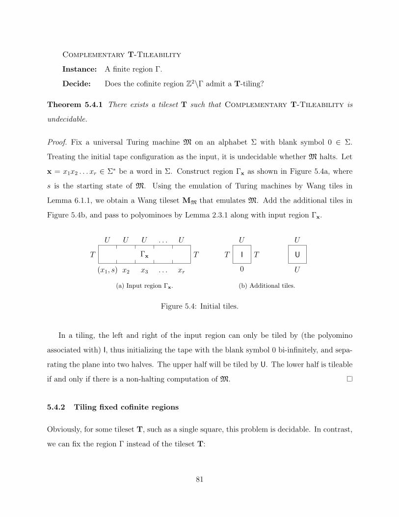
Complementary T-Tileability

Instance: A finite region Γ.

Decide: Does the cofinite region Z2\Γ admit a T-tiling?

Theorem 5.4.1 There exists a tileset T such that Complementary T-Tileability is

undecidable.

Proof. Fix a universal Turing machine M on an alphabet Σ with blank symbol 0 ∈ Σ.

Treating the initial tape configuration as the input, it is undecidable whether M halts. Let

x = x1x2 . . . xr ∈ Σ∗ be a word in Σ. Construct region Γx as shown in Figure 5.4a, where

s is the starting state of M. Using the emulation of Turing machines by Wang tiles in

Lemma 6.1.1, we obtain a Wang tileset MM that emulates M. Add the additional tiles in

Figure 5.4b, and pass to polyominoes by Lemma 2.3.1 along with input region Γx.

Γx

(x1, s) x2 x3 xr

U U U U

. . .

. . .

T T

(a) Input region Γx.

T

U

0

TI

U

U

U

(b) Additional tiles.

Figure 5.4: Initial tiles.

In a tiling, the left and right of the input region can only be tiled by (the polyomino

associated with) I, thus initializing the tape with the blank symbol 0 bi-infinitely, and sepa-

rating the plane into two halves. The upper half will be tiled by U. The lower half is tileable

if and only if there is a non-halting computation of M.

5.4.2 Tiling fixed cofinite regions

Obviously, for some tileset T, such as a single square, this problem is decidable. In contrast,

we can fix the region Γ instead of the tileset T:

81

Γ-Complementary Tileability

Instance: A tileset T.

Decide: Does the region Z2\Γ admit a T-tiling?

Theorem 5.4.2 Γ-Complementary Tileability is undecidable for any finite simply

connected7 region Γ.

In particular, even if we fix Γ as a single square, denoted [1 × 1], this problem is still

undecidable.8

Sketch of proof. We modify Complementary Tileability to have a fixed starting region.

Indeed, suppose we are given an instance consisting of a tileset T and a region Γ. Let T′ be

obtained by passing T∪Γ to Wang tiles and back to polyominoes via Lemma 2.3.1. Scale

all these tiles by a factor of 2, and then remove a single square from the tile Γ′ corresponding

to Γ. Note that Z2\[1× 1] admits a T′-tiling if and only if Z2\Γ admits a T-tiling. Indeed,

by passing to Wang tiles and back, these tiles automatically align in a dilated integer lattice

grid in any tiling. Since all tiles were dilated by a factor of 2, if Γ′ is not used, there is no

way to tile around the [1 × 1] unit square. On the other hand, every occurrence of Γ′ will

leave a [1 × 1] square uncovered. Thus Γ′ will be used precisely once, matching the square

at where it was removed. This transforms the original complementary tiling problem to one

with fixed input region [1× 1].

Fixing Γ as something else is similar. Indeed, let S be a large [N ×N ] square containing

Γ, such that S ′ = S\Γ is connected. It is possible that S ′ is not simply connected, in which

case we can break S ′ into two s.c. pieces that will interlock with each other only. Given an

instance T of [1 × 1]-Complementary Tileability, scale all tiles in T by a factor of N

to obtain an equivalent [N × N ]-Complementary Tileability problem. Now add (the

7Simple connectivity is necessary. Indeed, if Γ has a missing unit square in its interior, then its complementis tileable if and only if the tileset contains a single unit square.

8This is not surprising, since tiling the entire plane (Γ = ∅) is undecidable [Ber66]. In fact, the maindifficulty was the lack of a starting point. The case we consider is essentially the origin-constrained versionof tileability, which is undecidable [Wan63]. We include a sketch for completeness.

82

two pieces of) S ′ to the scaled tileset, reducing to Γ-Complementary Tileability, as

desired.

5.4.3 Tiling cofinite regions with rectangles

On the positive side, somewhat surprisingly, when the tileset consists only of rectangles, the

most general case (with neither the region nor the tileset fixed) is actually decidable.

Complementary Tileability with Rectangles

Instance: A region Γ and a tileset R of rectangles.

Decide: Does the region Z2\Γ admit a R-tiling?

Proof of Theorem 5.1.4. We first describe the algorithm. Suppose we are given a region Γ

and a tileset T consisting only of rectangles. Let A be the smallest rectangular region that

contains Γ in its interior. Place tiles to cover A (where tiles are allowed to protrude outside

of A), such that Γ is uncovered. Formally, find a region B ⊃ A and a tiling of B\Γ. Even

though this may look like an infinite problem with B unspecified, note that it is really a

finite problem, since we can exhaustively search all local tilings around Γ. Either there is no

way to cover A while avoiding Γ, in which case there is no tiling of Z2\Γ, or we find such a

B and a tiling π of B\Γ, in which case the complement of Γ is tileable.

Indeed, we may assume that π is minimal in the sense that removing any tile will leave

parts of A uncovered. Consider the tiling π at the top boundary of A. It consists of some

rectangles sticking out, and some that tile A just right. Regardless, simply use each of these

rectangles to tile the infinite half-strip above each segment. Similarly, tile the three half-

strips from the other three edges. Now we are left with four quadrants, which are obviously

tileable.

83

5.5 Tiling indented quadrants with rectangles

Lemma 2.3.1 lists several classes of Tileability problems that are equivalent. Tiling with

rectangles is equivalent with the others for finite regions, but Theorem 5.1.4 puts an end to

the hope of extending the equivalence to cofinite regions. Here we present an equivalence for

special infinite regions, and use it to exhibit yet another undecidable result.

Lemma 5.5.1 Given a (Wang) tileset T, it is undecidable whether the (white) fourth quad-

rant is T-tileable.

Proof. Take a Turing machine M with blank symbol b and initial state q0. Use Lemma 6.1.1

to get an associated tileset MM. Add the three initialization tiles from Figure 6.2, where ∅

signifies the white boundary of the fourth quadrant. Similar to the proof of Theorem 6.2.1,

we see that the fourth quadrant is tileable if and only if the Turing machine has a non-halting

computation when started on a 1-way infinite blank tape. Since that is undecidable (with

M varying as input), tileability of the quadrant is undecidable.

As usual, this result holds for a tileset of polyominoes by Lemma 2.3.1, where edges with

color ∅ are replaced by straight edges. Obviously, it makes no sense to ask the same question

for rectangular tiles. However, if we replace the boundary of the quadrant by periodic

rectilinear curves, then the problem becomes undecidable again. Call such a boundary a

periodically indented fourth quadrant.

Theorem 5.5.2 Given a periodically indented fourth quadrant Γ and a tileset R of rectan-

gles, it is undecidable whether Γ admits a R-tiling.

Proof. Take a set of polyominoes T. The reduction in Lemma 2.3.3 provides a set of rect-

angles R, and a linear-time function f that transforms a finite region Γ to another finite

region Γ′, such that Γ is T-tileable if and only if Γ′ is R-tileable. Explicitly, f takes each

unit-length edge of Γ and replaces it with a rectilinear curve to get Γ′. By feeding a single

vertical and a single horizontal edge to f , we get two rectilinear curves that can be used

84

to make the periodic boundary of an indented fourth quadrant. By carefully following the

proof of the bijective correspondence of T-tilings of regions and R-tilings of the transformed

regions, one can see that everything works for this specific infinite case as well. In particular,

in Sublemma 2.5.1, the unique R0-tiling of Γ0(r, c) was proved by placing tiles in the order

labeled in Figure 2.11. It is evident that this ordering extends to the infinite quadrant, and

the proof works verbatim.

We should note that the quadrant having a corner is essential when applying the proof

of Lemma 2.3.3 to this context. For example, this reduction does not work for the half-

plane. Indeed, for that case, the sketch of Lemma 5.5.1 does not work, but can be fixed with

some additional ideas to prove the corresponding lemma. The theorem, however, cannot be

salvaged, as the algorithm of Theorem 5.1.4 would apply with some minor alterations.

5.6 Augmentability

In the style of Rectangular Tileability, where we are interested if there is some finite

(rectangular) region from an infinite collection that is tileable by a given tileset, we consider

the following notion. A finite region Γ is augmentable if there is a finite s.c. region Γ′ ⊃ Γ

such that both Γ′\Γ and Γ′ are tileable.

Augmentability

Instance: A tileset T and a region Γ.

Decide: Is Γ augmentable by T?

As above, we can fix either T or Γ in the input (obviously not simultaneously). We have

the following result:

Theorem 5.6.1 Augmentability is undecidable. Moreover, it remains undecidable even

when Γ is fixed. Similarly, there exists some tileset T such that Augmentability with T

fixed is undecidable.

85

Proof. We first prove undecidability in general, then briefly sketch how Γ or T may be fixed

at the end of the proof. Recall that it is undecidable whether a Turing machine with a 1-way

infinite tape halts. By convention, the machine head starts at the left end of the tape, where

the input is written. Fix a Turing machine M on an alphabet Σ, with blank symbol 0 ∈ Σ,

and starting state s. Let MM denote the associated tileset of machine tiles afforded by

Lemma 6.1.1. Let BM be the tileset of border tiles defined in Figure 5.5, consisting of T, TR,

L, R, BL, and BR, Lx, Rx, and Hx,q for x ∈ Σ and q a halting state of M. The tileset F of filler

tiles consists of those in Figure 5.6. Finally, replace unlabeled edges in TM = MM∪BM∪F

with four new colors depending on which way each edge faces. By abuse of language, we will

continue to refer to these four colors on the boundary as white, with the understanding that

the white colors do not match, and thus the border tiles can only be used on the boundary

of a tiling and not in its interior. This finishes the construction of the tileset T = TM.

Γx

L (x1, s) x2 x3 xr. . .

T T

0

TT T

R

TR

L

L

VL V

R

R

R

L

x

LLx L

(x, q)

RHx,q R

x

RRx

L

LBL R

R

BR

Figure 5.5: Border tiles BM.

Let x = x1x2 . . . xr ∈ Σ∗ be a word in Σ. Construct region Γ = Γx as shown in Fig-

ure 5.5, where s is the starting state of M, and the white colors are subject to the same

aforementioned replacement treatment. It remains to show that Γx is augmentable by TM

if and only if M halts on input x.

86

L′

T ′TL′ T ′

H ′

T ′T′ T ′

R′

TR′

L′

L′

V ′L′ V ′

H ′

H ′

V ′C′ V ′

R′

R′

R′

L′

B′BL′ B′

H ′

B′B′ B′

R′

BR′

Figure 5.6: Filler tiles F.

Γx T T T TR

space-time diagram of a halting computation

(x, q)

L R

L R

L R

L R

Hx,qL• L• L• R• R• R• R•BL BR

Figure 5.7: Tiling of Γ′\Γ.

87

First, suppose M halts on input x. Take a tiling representing the space-time diagram

of a halting computation. By definition, the top boundary color sequence of the tiling is x,

possibly with blank symbol 0 repeated on its right. We may therefore place Γ above the

space-time diagram, with tiles T to its right (see Figure 5.7). Now we surround the region

by the other border tiles to get a white rectangular region Γ′. Of course, the bottom is tiled

by Hx,q, which matches the state symbol in the last row of the space-time diagram, and with

L• and R• tiles on the sides, where • denotes some unspecified symbol from Σ. We thus get

a tiling of Γ′\Γ automatically. Notice that since Γ′ is a white rectangle, it is tileable by the

filler tiles F ⊂ TM, as desired.

Conversely, suppose Γx is augmentable by TM. Since no tiles could be immediately above

or to the left of Γ, Γ′ matches the upper left corner of Γ. Thus in any tiling of Γ′, the space

currently occupied by Γ must be tiled by filler tiles. Note that as the filler tiles can only be

adjacent to other filler tiles, and since Γ′ is (simply) connected, Γ′ is tileable by filler tiles

alone. Of course, tilings of Γ′\Γ must not use filler tiles, as they cannot be adjacent to Γ.

This means the boundary of Γ′ must be colors common to both filler and non-filler tiles,

meaning that Γ′ is a white rectangle. The only way to tile Γ′\Γ is by using the border tiles

as shown in Figure 5.7, with precisely one Hx,q somewhere. Since the interior cannot utilize

border tiles, it must be tiled by the machine tiles MM alone. Thus it emulates a computation

starting from x, potentially followed by finitely many blank symbols, and ending at a halting

state (forced by the presence of a border tile Hx,q on the bottom boundary) after finitely

many steps, as desired.

We may interchange the role of Γx and TL′, adding Γx to the tileset and removing TL′ to

be used as the input region. This shows that Augmentability remains undecidable even

when Γ is fixed. On the other hand, by fixing M as some Universal Turing machine, we see

that there is some fixed T such that Augmentability is undecidable.

88

5.7 Final remarks and open problems

5.7.1

Tileability of a given finite region is decidable simply by exhaustive search. In this context,

tileability of finite regions by a finite tileset is NP-complete [Lew78].9 This is true even

when the tileset is fixed as a horizontal bar hn of n squares and a vertical bar vm of m

squares, n ≥ 2 and m ≥ 3 [BNRR95].10 However, when the region is simply connected

(s.c.), tileability by hn, vm can be determined in linear time [KK92].11 By comparing

these results, it is apparent that simple connectivity makes a difference. This is in part

due to Thurston’s height function approach [Thu90] and techniques in combinatorial group

theory developed by Conway and Lagarias [CL90]. Using these methods, Remila showed

that tileability of s.c. regions is quadratic for any two fixed rectangles [Rem05]. Perhaps

surprisingly, there is a finite set of rectangular tiles such that tileability of s.c. regions is

NP-complete (see Chapter 2). On the other hand, tileability of a rectangular region for a

fixed set of tiles can be determined in linear time (see below). Of course, if the rectangular

region is unspecified, undecidability returns. In a related direction, it is undecidable whether

a tileset is a code [BN03], i.e., every tileable finite region is uniquely tileable.

5.7.2

Theorem 5.1.2 leads to some curious consequences.

Theorem 5.7.1 ([DK75]) Given a tileset T, there is a tileset T′ consisting only of rectan-

gular tiles such that T and T′ tile the same rectangular regions.

9This was also indicated in an unpublished manuscript by Garey, Johnson, and Papadimitriou; see [GJ79,Pap94].

10Note that everything is tileable if n = 1; if n = m = 2, it is a matching problem and thus is solvable inpolynomial time (see e.g. [LP09]).

11Whenever the tileset is fixed, the complexity of the running time is given in terms of the area of theinput region.

89

Note that T can tile some rectangle if and only if T′ is non-empty. As such, in light of

our main theorem, it is undecidable if T′ is non-empty and, a fortiori, T′ is not computable

from T. Indeed, while the proof in [DK75] seems purely existential, now there is proof that

it cannot be made constructive.

Theorem 5.7.2 ([LMP05]) Tileability of an [n×m] rectangle by a fixed tileset of rectangles

can be determined in time O(log n+ logm).

Combining the two results, we see that there is a linear time algorithm for testing tileabil-

ity of rectangles for any fixed tileset. Again, the main theorem proves that the linear time

algorithm afforded by combining [DK75] with [LMP05] cannot be algorithmically determined

if the tileset is not fixed in advance. In the next subsection, we outline another consequence

regarding the growth of certain functions.

5.7.3

For a polyomino P that tiles some rectangle, Klarner defined the order h(P) of P as the

minimum number of copies it takes to tile some rectangle [Kla69], and conjectured that there

is no polyomino of order 3, which has since been confirmed [SW92]. There are polyominoes

of order 4s for each s ∈ N [Gol89], but no non-rectangular polyomino whose order is odd12

is known, and their existence is an open question (see e.g. [GO04, §15]).

For convenience, let us set h(P) = 0 if P does not tile any rectangle, and let

f(n) = maxh(P) : |P| = n,

where |P| is the area of (the shape of) P. If it is computable or bounded above by a

computable function, then Rectangular Tileability for a single polyomino would be

decidable. Indeed, if there exists a computable function g(n) such that f(n) ≤ g(n), then

given P, simply try tiling all rectangles with areas up to g(|P|). This is a finite process that

terminates. If no tilings are found, then P does not tile any rectangle. There are several

12One should not confuse this with the notion of odd order, also introduced in [Kla69].

90

claims that the problem is decidable (thus the function f(n) is computable), but to our best

knowledge (see e.g. [AS10]), no proofs are currently known.

Along the same vein, let h(T) denote the minimum area of a rectangle tileable by a

tileset T, and set h(T) = 0 if T does not tile any rectangle. Note that when T = P is a

single polyomino, we have h(P) = h(P)/ |P|. Similarly, define

f(n) = maxh(T) : T has total area n.

Corollary 5.7.3 The function f(n) grows faster than any computable function, e.g., the

fast-growing Ackermann function.

Proof. This follows immediately from the undecidability of Rectangular Tileability

(Theorem 5.1.2).

5.7.4

Wang conjectured that there is no aperiodic tileset of Wang squares [Wan61]. If this conjec-

ture were true, Tileability for Wang squares would be decidable. Indeed, simply enumerate

all tilings of [N ×N ] squares, N = 1, 2, . . .. Either some square admits no tiling (and thus

the plane is not tileable), or at some point a finite fundamental domain will be found that

can be used to tile the whole plane periodically. Berger disproved the conjecture by showing

the undecidability of this tileability problem [Ber66]. As a consequence, there is an aperiodic

tileset of Wang squares. After a series of reductions in the number of Wang squares, the

current record is 13 [Cul96].

5.7.5

Reducing the number of tiles in an aperiodic tileset has been the subject of much effort.

The famous Penrose tilings derive aperiodicity from a pair of tiles [Pen74]. Here a tile is

a geometric shape that can be rotated (and reflected) in addition to translation. These

tilings inherit aperiodicity from quasicrystals and thus do not admit transformations onto

91

lattices. Socolar and Taylor constructed a single tile on the hexagonal lattice that exhibits

aperiodic behavior when external matching rules are enforced [ST11]. Since the matching

rules span non-adjacent tiles, encoding this as a geometric tile (with no external matching

rules) necessarily resulted in a tile whose interior is disconnected. There seems to be no

obvious way to circumvent this in the plane.

Returning to the square lattice, it is unknown whether there is a single polyomino that

could force aperiodic behavior. Decidability of whether a polyomino admits a tiling (or a

periodic tiling) of the plane is open. However, there is a polynomial-time algorithm for

deciding whether a given polyomino admits an isohedral tiling [KV99], i.e., a tiling where

the group of isometries acts transitively on the tiles thereof. If only translations are allowed

on a single polyomino, Tileability of the plane is decidable [BN91], and an algorithm with

running time quadratic in the boundary length is known [GV07].

5.7.6

Let us consider tilings of finite regions. Traditionally, the use of coloring maps is a main

tool for proving non-tileability (see [Gol65]). It actually proves the non-existence of signed

tilings, i.e., a finite collection of tiles with ±1 weights such that the weights of tiles covering

each square sum to 1 inside the region and 0 outside (see [CL90]). Conversely, when there

are no signed tilings, there is a coloring argument that certifies it (see [Pak00]). This is not

true for ordinary tilings. Indeed, there are non-tileable regions that admit signed tilings,

thus proving non-tileability using this method is impossible for those regions.

The notion of augmentability considered in Section 5.6 can be formulated in this language

of signed tilings, by requiring tiles with equal weights to be pairwise disjoint. Augmentability

is therefore a (proper) intermediate notion between tileability and signed tileability. That

is, tileable regions are augmentable, and augmentable regions are signed tileable. Moreover,

the implications are not bidirectional [Kor04].

92

5.7.7

There are instances where results of tilings in the plane do not extend to higher dimen-

sions. For example, the number of tilings of a finite region by dominoes can be counted

efficiently in the plane, but is #P-complete in higher dimensions (see Chapter 4). However,

all of the results in this chapter extend easily to higher dimensions. Indeed, Rectangular

Tileability extends by simply endowing each 2D tile with height 1 in the remaining di-

rections. The results involving Turing machines can also be easily extended in the obvious

manner. Extending Complementary Tileability with rectangles to higher dimensions

is only slightly trickier. A brick in Zn is the Cartesian product of n intervals.

Theorem 5.7.4 It is decidable whether the complement of a given finite region Γ in Zn is

tileable by a given tileset T consisting only of bricks.

Proof. We follow the same proof as given in Subsection 5.4.3. Indeed, let A be the smallest

brick region that contains Γ in its interior. Find a region B ⊃ A and a tiling π of B\Γ. This

task is finite, and is possible if and only if Zn\Γ is tileable.

Indeed, assume that π is minimal. It remains to exhibit a tiling of Zn\B. For a brick

in π, call its facet free if it is entirely on the boundary of B. Suppose a brick centered at

coordinates x has a free facet. Its cone is the set of copies of the brick centered at x + Z+v,

where v is the width vector from the opposite facet to the free facet, and Z+ = 0, 1, 2, . . ..

More generally, if a brick centered at x has k free facets, with corresponding width vectors

v1, . . . ,vk, define its cone as the set of copies of the brick centered at x+ Z+v1 + . . .+ Z+vk.

(This works even if some pairs of free facets are opposite one another.) It is easy to see that

the cones of the bricks partition Zn\Γ.

Another direction of generalization is to consider other infinite regions with reasonable

finite descriptions. For example, consider a periodic perforated plane, where there are holes

occurring throughout the region in some periodic manner. This may lead to interesting

results like Theorem 5.5.2.

93

One could also ask for the running-time complexity of the algorithm described in the

proof of Theorem 5.1.4. In particular, what happens if the tileset is the (horizontal and

vertical) dominoes?

94

CHAPTER 6

Demonstrating the power of tiles by emulating Turing

machines

In this short chapter, we outline the classical technique of emulating Turing machines with

tiles, an idea mentioned in Subsection 2.7.2 and heavily used in Chapter 5. We then create

a tileset that tiles a quadrant uniquely while performing prescribed calculations.

6.1 Emulating Turing machine with tiles

Consider a Turing machine M on an alphabet Σ and let Q denote its set of states. We refer

to the elements of Σt (Σ×Q) as colors, where (x, q), x ∈ Σ and q ∈ Q, are called compound

colors. A configuration of M is represented as a (possibly infinite) sequence of colors, where

all but finitely many are the blank symbol b ∈ Σ. Moreover, there must be precisely one

compound color (x, q). Reading (x, q) as x, this sequence represents the contents of the

tape. The head of the machine is at the position of (x, q), and the current state is q. Such a

sequence of colors (corresponding to a valid configuration) is called valid. A row of (possibly

infinite) Wang squares is valid if their bottom colors form a valid sequence. We say a set

of Wang squares W emulates M if given a valid row of Wang squares, and a second row of

Wang squares below it, the second row represents a configuration obtained from the previous

one after one time step (and therefore is a valid row). Moreover, if M is non-deterministic,

all possible next configurations are realizable by such tilings. This way, a tiling with W is a

space-time computation diagram of M, given that it starts with a valid row. Furthermore,

all possible space-time diagrams are realizable as tilings.

95

Lemma 6.1.1 There is a computable tileset MM of Wang squares that emulates a given

Turing machine M.

Proof. This construction is classical and well known (see e.g. [LP97, §6]). For completeness

and also to fix an explicit construction, we provide a proof here.

Let M = (Q, q0,Σ, b, δ) be a deterministic Turing machine, with a finite set Q of states

that contains a starting state q0 ∈ Q, a finite alphabet Σ that contains a blank symbol b ∈ Σ,

and a transition function δ : Σ × Q → Σ × Q × L,R. There is a tape with a horizontal

row of cells, each cell holds precisely one symbol from Σ. The tape has a left-most cell, but

extends infinitely to the right. At the beginning, every cell contains the blank symbol b. The

head of the Turing machine starts on the left-most cell, in starting state q0. At each step,

the head reads the symbol a from the cell at which it is located. Suppose the current state

is q, and δ(a, q) = (a′, q′, D). The head replaces the content of the cell by a′, and enters

state q′. Moreover, it moves to the left or right on the tape depending on if D is L or R.

Let τ(w, ns, e) denote a Wang tile whose north, east, south, and west colors are n, e, s,

and w, respectively. To emulate M, we introduce the following tiles (see Figure 6.1). For

each a ∈ Σ, add a Wang tile τ(V, aa, V ), where V is a new symbol. For each a ∈ Σ and

q ∈ Q, if δ(a, q) = (a′, q′, L), introduce τ((q′, L), (a,q)a′ , V ). Analogously, if δ(a, q) = (a′, q′, R),

add τ(V, (a,q)a′ , (q

′, R)). Finally, add τ((q, R), a(a,q)

, V ) and τ(V, a(a,q)

, (q, L)). To summarize,

V

a

a

V V

a

(a, q)

(q, L) (q′, L)

(a, q)

a′

V

V

(a, q)

a′

(q′, R) (q, R)

a

(a, q)

V

Figure 6.1: Machine tiles MM.

96

the horizontal colors are Σt (Σ×Q), and the vertical colors are V and Q×L,R. We refer

to the colors involving Q as compound colors, and call these tiles the machine tiles MM.

Let us look at the top colors of a row of tiles. Suppose it has one compound color (a, q),

and all others are not. The color sequence depicts contents of the tape, if we read (a, q)

as a. The location of (a, q) indicates the position of the head, and q is the current state.

In this manner, the color sequence encodes precisely the Turing machine at some time step.

The bottom colors of this row of tiles will be the Turing machine at the next step. Indeed,

suppose δ(a, q) = (a′, q′, L). By construction, there is precisely one tile that has top color

(a, q). It has bottom color a′, corresponding to replacing a with a′ at the location of the head.

The left color is (q′, L), which causes the tile on the left to be precisely τ(V, c(c,q′)

, (q′, L)),

meaning now the head has moved left one tile. For all other tiles, if the top color is c, it must

be the tile τ(V, cc, V ). Indeed, the other options would involve having a compound colors on

a vertical side, forcing an adjacent tile to have a compound color on top, a contradiction.

Note that for a non-deterministic Turing machine, where the transition table is not

necessarily a function, we simply add tiles corresponding to each possible transition. We

omit the simple details.

6.2 Tiles that do something specific, e.g., calculate the digits of π

In this section, we illustrate the power of tiles by creating a set of tiles that encode the digits

of π in some precise sense. Of course, there is nothing too special about π, and we can

encode some other number that we know how to calculate well.

Theorem 6.2.1 There exists a tileset T that admits a unique tiling of the fourth quad-

rant, such that the top row of this tiling uses tiles τ0, τ1 ∈ T, and the sequence of 0 and 1

corresponding to the tiles used is the binary expansion of π.

The idea is to encode a specific Turing machine M using a set W of Wang tiles, and then

pass to a set of tiles as usual.

97

Let M be a Turing machine satisfying the following:

(i) when started on a blank tape, the head never moves left past the starting position,

(ii) its alphabet Σ contains immutable symbols 0 and 1, that is,

(iii) if it writes 0 or 1 on the tape, it never tries to change it at a later step, and

(iv) each cell on the tape is eventually marked with 0 or 1, which forms the binary expansion

of π − 2 with the decimal point omitted.

The existence of M can be proved by explicitly constructing such a Turing machine, and

is essentially guaranteed by the Church–Turing thesis. Take such an M and consider the

machine tiles MM afforded by Lemma 6.1.1.

Suppose we are to tile the fourth quadrant, whose boundary color is denoted ∅. Introduce

three initialization tiles τ∅ = τ(∅, ∅b,∅), τI = τ(∅, b

L, (q0, R)), and τL = τ(∅, L

L, V ). Notice

∅

∅

b

∅τ∅

∅

b

L

(q0, R)τI

∅

L

L

VτL

Figure 6.2: Initialization tiles for tiling the fourth quadrant.

that the top row is uniquely tiled by using only τ∅, and the left column is uniquely tiled

by τ∅, τI , followed by τL repeatedly. Moreover, these three tiles cannot be used anywhere

98

else. Thus we have initialized a decorated quadrant with top color b, and left color sequence

(q0, R), V, V, . . .. This exactly allows the machine tiles to start computation on a blank tape

with initial state q0, as desired.

After encoding the Turing machine M as a set of Wang squares MM and adding a few

tiles to initialize, we are ready to employ one last trick to make the digits of π materialize at

the top row. For each machine tile τ(w, ns, e), replace it with two tiles τ(w, (n,i)

(s,i), e), i ∈ 0, 1,

except when s ∈ 0, 1, in which case we only add the tile with s = i. We call i the parity of

the tile. By construction, each column of a tiling by these tiles must have consistent parity.

This is possible since we will not have 0 or 1 occurring in the same cell in the Turing machine

computation, as they are immutable. On the other hand, since each cell eventually is written

with 0 or 1, the parities are forced. In other words, we have successfully lifted the output of

the Turing machine computation all the way to the top!

It remains to make slight modifications to the initialization tiles as follows: replace τ∅

with τi = τ(∅, ∅(b,i)

,∅), i ∈ 0, 1, change τI to τ(∅, (b,1)L, (q0, R)), and leave τL unchanged.

Note that this hard codes the corner tile to be τ1, which is why we chose a Turing machine

that calculates the binary expansion of π − 2. The unique tiling of the quadrant is now

restored, and the top row consists of τ0 and τ1, whose indices form the binary expansion of

π, as desired.

99

CHAPTER 7

The interplay between tilings and cellular automata

The theory of cellular automata is rich and has attracted a lot of study (see e.g. [Kar05]

for standard terminology and a survey of results), including the search for simple universal

systems [Coo04, Oll02]. This is akin to the efforts in finding small universal Turing ma-

chines [NW09, Rog96]. In this chapter, we describe easy constructions to emulate cellular

automata with tiles (Section 7.1) and vice versa (Section 7.3). In Section 7.2, we emulate the

so-called Rule 110 cellular automaton efficiently using this technology. A notion of function-

pair universality is introduced in Section 7.4, which promises conjectural improvements of

the number of rectangles needed in Theorem 2.1.1. Finally, we provide a brief reasoning as

to the hope of such conjectural improvements being possible (Section 7.5). In this chapter,

most proofs are merely sketches, and all cellular automata are 1-dimensional.

7.1 Emulating cellular automata with tiles

A cellular automaton A of rank n consists of a finite set of states Σ and a (local) update rule

fA : Σn → Σ. Let the global update function ΦA : ΣZ → ΣZ be the action of applying fA

synchronously everywhere. Given a cellular automaton with neighborhood consisting of cells

at most distance d away (i.e., n = 2d+ 1), we construct the following set of Wang squares.

For each (x−d, . . . , x0, . . . , xd) ∈ Σn, we introduce a tile whose left and right colors are

(x−d, . . . , xd−1) and (x−d+1, . . . , xd), respectively, the top color is x0, and the bottom color is

f(x−d, . . . , xd). This construction yields sn Wang squares.

100

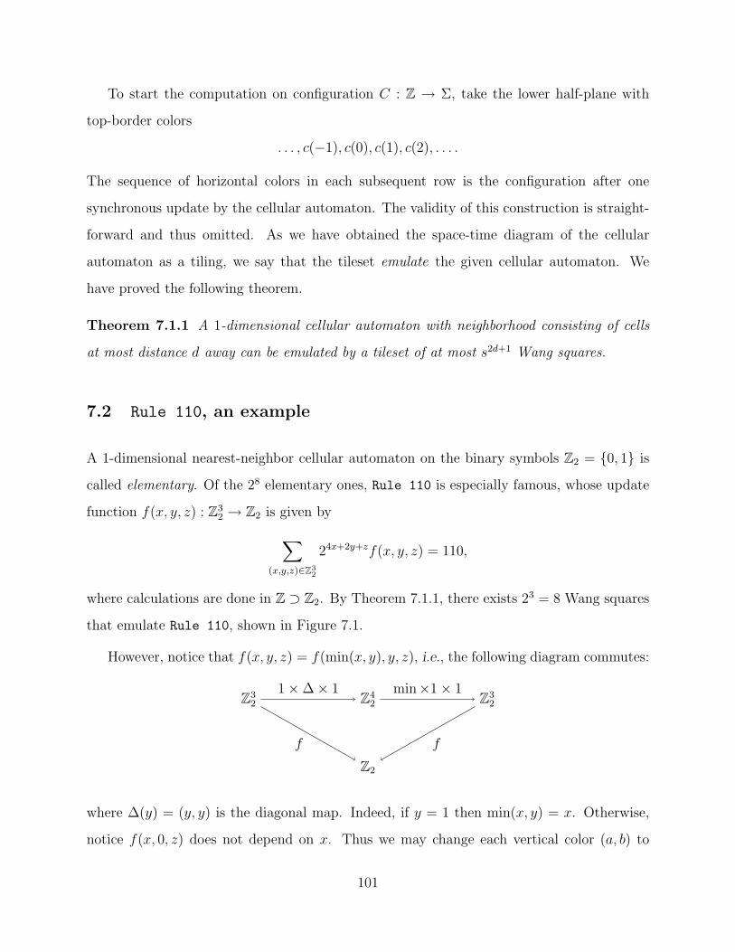
To start the computation on configuration C : Z → Σ, take the lower half-plane with

top-border colors

. . . , c(−1), c(0), c(1), c(2), . . . .

The sequence of horizontal colors in each subsequent row is the configuration after one

synchronous update by the cellular automaton. The validity of this construction is straight-

forward and thus omitted. As we have obtained the space-time diagram of the cellular

automaton as a tiling, we say that the tileset emulate the given cellular automaton. We

have proved the following theorem.

Theorem 7.1.1 A 1-dimensional cellular automaton with neighborhood consisting of cells

at most distance d away can be emulated by a tileset of at most s2d+1 Wang squares.

7.2 Rule 110, an example

A 1-dimensional nearest-neighbor cellular automaton on the binary symbols Z2 = 0, 1 is

called elementary. Of the 28 elementary ones, Rule 110 is especially famous, whose update

function f(x, y, z) : Z32 → Z2 is given by∑

(x,y,z)∈Z32

24x+2y+zf(x, y, z) = 110,

where calculations are done in Z ⊃ Z2. By Theorem 7.1.1, there exists 23 = 8 Wang squares

that emulate Rule 110, shown in Figure 7.1.

However, notice that f(x, y, z) = f(min(x, y), y, z), i.e., the following diagram commutes:

Z32 Z4

2 Z32

Z2

1×∆× 1 min×1× 1

f f

where ∆(y) = (y, y) is the diagonal map. Indeed, if y = 1 then min(x, y) = x. Otherwise,

notice f(x, 0, z) does not depend on x. Thus we may change each vertical color (a, b) to

101

(1, 1)

1

0

(1, 1) (1, 1)

1

1

(1, 0) (1, 0)

0

1

(0, 1) (1, 0)

0

0

(0, 0)

(0, 1)

1

1

(1, 1) (0, 1)

1

1

(1, 0) (0, 0)

0

1

(0, 1) (0, 0)

0

0

(0, 0)

Figure 7.1: Emulating Rule 110 with 8 tiles.

(min(a, b), b) in the construction (see Figure 7.2, changes are underlined). This yields the

general tile

τ((min(x, y), y),y

f(min(x, y), y, z), (min(y, z), z)).

Thus we get six tiles, one for each x, y, z ∈ 0, 1 with x ≤ y.

(1, 1)

1

0

(1, 1) (1, 1)

1

1

(0, 0)

(0, 1)

1

1

(1, 1) (0, 1)

1

1

(0, 0) (0, 0)

0

1

(0, 1) (0, 0)

0

0

(0, 0)

Figure 7.2: Emulating Rule 110 with 6 tiles W6.

Corollary 7.2.1 There is a set W6 of 6 Wang squares that emulate Rule 110.

We can use these tiles in various ways. For example, by adding the initialization tiles

in Figure 7.3, the (white) third quadrant will admit a unique tiling showcasing the famous

picture of Rule 110 started with a single 1. In Figure 7.4, each tile with bottom color 0

(resp. 1) is drawn as a white (resp. black) pixel.

102

T

0

TI0 T

1

C C

R

(0, 0)

R

R

Figure 7.3: Tiles to initialize Rule 110 to fill the third quadrant.

Figure 7.4: Rule 110 filling the third quadrant started with a single 1.

103

Alternatively, we can add the tiles in Figure 7.5 to allow random initial configurations

for Rule 110 for the lower half-plane, say.

T

0

TI0 T

1

TI1

Figure 7.5: Tiles to introduce random initial configuration for Rule 110.

7.3 Emulating tiles with cellular automata

Since we can emulate cellular automata with tiles, we could emulate a specific universal

cellular automaton, in the hopes of reducing the size of our tilesets. For simplicity, we avoid

repeatedly defining “emulate” in various settings, implicitly appealing to standard literature

when the meaning is not clear from context.

A tileset of Wang squares is NW-deterministic if there are no two Wang squares that

have the same colors on their north and west edges as each other.

Lemma 7.3.1 A tileset of NW-deterministic Wang squares can be emulated by a cellular

automaton.

Proof. Denote the vertical and horizontal colors of the tileset V and H, respectively, and let

Σ = V t H. Define a nearest-neighbor cellular automaton on Σ with the following update

rule: for w ∈ V , let f(z, w, n) = s, where s is the south color of the unique tile1 with west

and north colors w and n, respectively; similarly, for n ∈ H, let f(w, n, z) = e, where e is the

east color of the same tile. This finishes the construction. Each tiling appears as a subset of

some space-time diagram of this cellular automaton (rotated by π/4).

There are several notions of universality in the theory of cellular automata. If a cel-

lular automaton can emulate any other cellular automata (of the same dimension), it is

1If no such tile exists, the update rule can be arbitrary, as that case will not be used in the emulation.

104

intrinsically universal. Intrinsic universality is strictly stronger than Turing computational

universality.

Corollary 7.3.2 There is a tileset of Wang squares that emulate any NW-deterministic

Wang squares.

Proof. Fix an intrinsically universal 1-dimensional cellular automaton A. For example,

[OR11] presents one with only 4 states (see also [Oll02]). Any tileset of NW-deterministic

Wang squares can be emulated by a cellular automaton (Lemma 7.3.1), which in turn can

be emulated by A, and is finally emulated with Wang squares (Theorem 7.1.1). Since A is

fixed, so is the resulting tileset.

Unfortunately, known examples of intrinsically universal cellular automata all lead to too

many Wang squares when emulating, thus foiling our plan. In the previous section, we saw

that, as an example, Rule 110 can be emulated with 6 Wang squares. However, though

Turing universal [Coo04], it is unknown whether Rule 110 is intrinsically universal. In the

following section, we outline a weaker form of universality that is sufficient for our purposes.

7.4 Function-pair universality of cellular automata

Let ⊕ denote string concatenation. A cellular automaton on alphabet Σ with global update

function Φ is function-pair universal if for all pairs f, g : Ω2 → Ω, where Ω is an arbitrary

alphabet, we have injective “encoding function” h : Ω → Σt for some t ∈ N, “time dilation

factor” N ∈ N, and “program” words a, b, c, d ∈ Σ∗, such that

ΦN(a⊕ h(x)⊕ b⊕ c⊕ h(y)⊕ d) = c⊕ h f(x, y)⊕ d⊕ a⊕ h g(x, y)⊕ b (*)

for all x, y ∈ Ω, regardless of the states of the rest of the cellular automaton. The following

theorem is important, albeit obvious.

Theorem 7.4.1 Every intrinsically universal cellular automaton is function-pair universal.

105

This demonstrates the existence of function-pair universal cellular automata. We now

show that they are sufficiently powerful for our needs.

Theorem 7.4.2 Any tileset W of NW-deterministic Wang squares can be emulated by any

function-pair universal cellular automaton A.

Proof. Fix some W and A as in the statement. Let Ω be the set of colors used in W, and let

f(w, n) and g(w, n) be the south and east colors, respectively, of the unique tile with west

and north colors w and n, respectively. By function-pair universality, there are programs

a, b, c, d ∈ Σ∗, encoding function h, and time dilation factor N such that (*) is satisfied. We

may now represent an NW-staircase boundary by encoding the colors by h, punctuated by

the programs a, b, c, and d. The output of running A for N steps would be (an encoding of)

the colors on the next diagonal of the unique tiling by W. Moreover, the programs c and

d would trade places with the programs a and b, allowing the computation of the next row

using the new boundary.

We say that function-pair universality is tight if for Ω = Σt, (*) is satisfied with the

identity map as h. Now we aim to emulate a tileset whose tiling problem is known to be

NP-complete.

Lemma 7.4.3 There exists a NW-deterministic Wang tileset W and tiles τ0, τ1, appearing

only on the boundary, such that Simply Connected W ∪ τ0, τ1-Tileability is NP-

complete.

Proof. Consider the set W15 constructed in the proof of Lemma 3.1.1. It is not NW-

deterministic for several reasons, including the tile Ri that transmit information to the left,

the tile Xij that transmit information upwards, and Vi that initiates the computation. Be-

sides the last one (which is needed for the tiling to have computational power), the others

are easily fixed.

Indeed, we modify W15 to obtain Wd. The tiles are drawn in Figure 7.6, where the

symbols i, j, and k, which appear in the subscripts of the tiles can be replaced by 0 or 1, and

106

the other symbols are distinct colors. First, we trade the roles of L and R so L propagates

signal to the southeast while R goes due south. We make the X tiles appear when L2 would

have intersected with an R2 tile. To solve the X problem, we shift everything down by one

on a column with R. That is, after starting with R1, the signal of the current row will be

propagated downward (coupled with r). This signal will be exhibited on the next row by

R2, which also shifts a signal down, and similarly onwards with many R2 tiles. Then X1 will

do the same, but summons X2, which allows the signal in this row to pass through without

change. Then X3 displays the signal from two rows above (thus effectively crossing two

signals over), and continue the chain of moving the signals down one row by repeated use of

X3 tiles. Finally, the X4 tile is used for the last tile, which has west boundary ∅. If there

are n variables, the old region for W15 is a trapezoid of height 3n. Now the region starts

with 3n rows, becomes 3n + 1 rows in a column whose top color is r, and is followed by 3n

rows shifted one row down. This is repeated as many times as the color r is used on the

top boundary. The extra vertical edges resulting from the shifted boundary will be colored

by ∅.

It is pretty easy to break V and C tiles into Wang squares. Finally, we add in Fi from

W15 without modification. This completes the construction. Removing τi = V1i from Wd

yields a NW-deterministic tileset of Wang squares, as desired.

Theorem 7.4.4 Suppose there is a tight function-pair universal cellular automaton A

that can be emulated by a tileset W of n Wang squares. The tileset Wd constructed in

Lemma 7.4.3 can be emulated by adding two extra tiles to W.

Proof. Recall that the Wd is not NW-deterministic because of τi. We change tile τi to

have color i′ instead of ∅ on the west edge. Represent all the colors as different strings of

Ω = Σt, where 0′ and 1′ are the same string except for one bit. Apply the construction in

Theorem 7.4.2. Finally, add a special pair of tiles (cf. Figure 7.5) that can be used on the

boundary to change a bit, representing either τ0 or τ1 as the starting tile for computation.

107

i

`

o

(`, i)L1i

(`, i)

o

`

iL2i

(a) L tiles.

i

r

(r, i)

∅R1i

i

(r, j)

(r, i)

jR2ij

(b) R tiles.

(`, i)

(r, j)

(p, i)

jX1ij

i

(p, j)

(x, j)

iX2ij

i

(x, j)

(x, i)

jX3ij

∅

(x, j)

o

jX4j

(c) X tiles.

∅

v0

(v1, i)

iV1i

∅

(v1, i)

(v2, i)

iV2i

∅

(v2, i)

v0

iV3i

(d) V tiles.

i

c0

(c1, i)

∅C1i

j

(c1, i)

(c2, i+ j)

∅C2ji

k

(c2, 1− k)

c0

∅C3k

(e) C tiles.

Figure 7.6: Tiles for constructing Wd.

108

Recall that Rule 110 can be emulated by 6 tiles (Corollary 7.2.1). Combining with the

series of results in this section, we get the following conjectural result.

Corollary 7.4.5 If Rule 110 is tight function-pair universal (or intrinsically universal),

then it can emulate Wd with 8 Wang squares W8. As such, Simply Connected W8-

Tileability is NP-complete.

Finally, this leads to another conjectural improvement on the number of rectangles needed

in Theorem 2.1.1.

Corollary 7.4.6 If Rule 110 is tight function-pair universal, then there exists a set R51

of 51 rectangles such that Simply Connected R51-Tileability is NP-complete.

Proof. Apply Lemma 3.2.1 to the tileset W6 in Figure 7.2 that emulates Rule 110. By

adding two tiles with the width of the h tiles but a height too tall to fit in anywhere else

(one needs to trace through the uniqueness proof in Sublemma 2.5.1 to verify this), we can

make it possible for colors 0 and 1 to appear on the boundary without being specified. This

removes the need for emulating W8. By counting carefully the number of resulting tiles (as

in Theorem 3.3.2), we see that W6 yields 23 tiles before doubling, thus giving a total of

23 · 2 + 3 + 2 = 51 tiles.

7.5 Using Turing computation universality of cellular automata

Let M be a Turing machine defining a partial recursive function Ψ : T → T , where T is

some countable set of Turing machine tapes. A cellular automaton A on alphabet Σ with

global update function Φ emulates M if there exists mappings h : T → ΣZ and g : ΣZ → T ,

a finite “program” word p ∈ Σ∗, and a “time dilation factor” N ∈ N, so that

Ψ(x) = g ΦN(h(x)⊕ p) (†)

whenever Ψ(x) is defined. If this can be done for all M, then A is Turing (computation)

universal.

109

Towards evidence of function-pair universality, we consider this following simplification.

Fix a Turing universal cellular automaton A. Let f : Σt → Σt be some total function. Find

p and N such that

ΦN(x⊕ p) = f(x)⊕ p.

We sketch an argument below to show how this may be accomplished by using Turing

universality.

For each string q, there is a Turing machine Mq calculating Ψq : Σt → Σt+|q| given by

Ψq(x) = f(x)⊕ q,

where |·| denotes the length of a string. By universality of A, there exists (h, g, p,N) for each

q satisfying (†). For simplicity, suppose that h and g are identity (so T = ΣZ), N = N(t)

does not depend on f , and denote the p obtained by each q as p(q). We thus obtain

ΦN(x⊕ p(q)) = Ψq(x) = f(x)⊕ q.

We wish to find a fixed point e such that p(e) = e. We cannot do this, but we can use results

from logic to do something that is sufficient for our purpose:

Theorem 7.5.1 (Second Recursion Theorem) If F is a total computable function then

there is an index e such that ϕe = ϕF (e), where ϕe is the partial recursive function with

Godel number e.

For each program p, associate a function

ϕp(x) = ΦN(|x|)(x⊕ p).

Note that by universality, ϕp enumerates all partial recursive functions. Thus we may apply

the Second Recursion Theorem with F = p to obtain an index e such that ϕe = ϕp(e).

Therefore we get

ΦN(|x|)(x⊕ e) = ϕe(x) = ϕp(e)(x) = ΦN(|x|)(x⊕ p(e)) = Ψe(x) = f(x)⊕ e,

110

as desired. In other words, there is a way to select a program e such that running the cellular

automaton A for N = N(t) steps transforms a string of length t to an arbitrary target string

of the same length. Moreover, the program e will appear in the right place for us to run the

computation again.

111

CHAPTER 8

Conjectural improvements on the number of rectangles

Lemma 2.3.3 establishes a bound of 2n2 + 4n + 2 rectangles, where n = 2k is double the

size of the input Wang tileset. The state of the art for this bound given in Lemma 3.2.1 is

5n + 3. This improvement is made by fixing the h and the v tiles and varying the w tile

instead (see Table 8.1). In the first section, we go back to the original setup and outline a

conjecture that would reduce the number of h and v tiles to constants without increasing

the number of w tiles. In the second section, we tackle the 4n bottleneck for the s tiles with

another conjecture, which is a strengthening of the first.

8.1 Alternate number theory component

A digraph G on [n] is a subset of [n]2. For this chapter, digraphs are loopless, i.e., (i, i) /∈ G

for any i ∈ [n]. Let a = (a1, . . . , an) ∈ Nn, N ∈ N, and D ⊂ N. We say (a, N,D) emulates a

digraph G if

(i) N > 1000 maxi ai, and

h and v w s f Sum

Lemma 2.3.3 2 · n2 1 4n 1 2n2 + 4n+ 2

Lemma 3.2.1 2 · 1 n 4n 1 5n+ 3

Conjecture 8.1.1 2 · 3 1 4n 1 4n+ 8

Conjecture 8.2.1 2 · 3 1 3 1 11

Table 8.1: Summary of the bounds on the number of rectangles obtained.

112

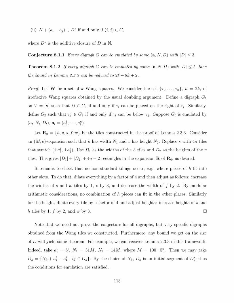
(ii) N + (ai − aj) ∈ D∗ if and only if (i, j) ∈ G,

where D∗ is the additive closure of D in N.

Conjecture 8.1.1 Every digragh G can be emulated by some (a, N,D) with |D| ≤ 3.

Theorem 8.1.2 If every digraph G can be emulated by some (a, N,D) with |D| ≤ `, then

the bound in Lemma 2.3.3 can be reduced to 2`+ 8k + 2.

Proof. Let W be a set of k Wang squares. We consider the set τ1, . . . , τn, n = 2k, of

irreflexive Wang squares obtained by the usual doubling argument. Define a digraph G1

on V = [n] such that ij ∈ G1 if and only if τi can be placed on the right of τj. Similarly,

define G2 such that ij ∈ G2 if and only if τi can be below τj. Suppose Gt is emulated by

(at, Nt, Dt), at = (a1t , . . . , a

nt ).

Let R0 = h, v, s, f, w be the tiles constructed in the proof of Lemma 2.3.3. Consider

an (M, e)-expansion such that h has width N1 and v has height N2. Replace s with 4n tiles

that stretch (±ai1,±ai

2). Use D1 as the widths of the h tiles and D2 as the heights of the v

tiles. This gives |D1|+ |D2|+ 4n+ 2 rectangles in the expansion R of R0, as desired.

It remains to check that no non-standard tilings occur, e.g., where pieces of h fit into

other slots. To do that, dilate everything by a factor of 4 and then adjust as follows: increase

the widths of s and w tiles by 1, v by 3, and decrease the width of f by 2. By modular

arithmetic considerations, no combination of h pieces can fit in the other places. Similarly

for the height, dilate every tile by a factor of 4 and adjust heights: increase heights of s and

h tiles by 1, f by 2, and w by 3.

Note that we need not prove the conjecture for all digraphs, but very specific digraphs

obtained from the Wang tiles we constructed. Furthermore, any bound we get on the size

of D will yield some theorem. For example, we can recover Lemma 2.3.3 in this framework.

Indeed, take ait = 5i, N1 = 31M , N2 = 14M , where M = 100 · 5n. Then we may take

Dk = Nk + aik − a

jk | ij ∈ Gk. By the choice of Nk, Dk is an initial segment of D∗k, thus

the conditions for emulation are satisfied.

113

8.2 Another alternate number theory component

In this section, we provide a strengthening of Conjecture 8.1.1, where we prescribe some

structure to the a, N , and D that emulate a digraph G. We follow the notations from the

previous section.

Conjecture 8.2.1 Given digraphs G1 and G2, there exist

(i) an odd prime p,

(ii) a ≡ a′ ≡ b ≡ b′ ≡ 0 (mod 2), ab ≡ 2 (mod 3), a, b, b′ ≡ 0 (mod p), a′ ≡ 1 (mod p),

(iii) D1 ⊂ N consisting of multiples of 2p,

(iv) D2 ⊂ N consisting of odd multiples of 3p,

(v) ` > 0 and g : [n]→ N such that min g > `,

(vi) (p− 2)a′ > wd f ,

(vii) ht f odd multiple of 3p, wd f even and −2 (mod p),

(viii) sk = R(ka+ (k + 1)b, a′ + (k + 1)b′),

(ix) N1 = 2wd s` + wd f is a multiple of 2p, and N2 = ht f − 2ht s` is 1 (mod 6), and

(x) ai1 = wd sg(i) −wd s` and ai

2 = ht sg(i) − ht s`,

such that (at, Nt, Dt) emulates Gt. Moreover, this can be done with |D1| , |D2| ≤ 3.

The conditions in the statement of the conjecture may seem daunting, but that is because

we recorded exactly the modular arithmetic constraints needed to prove the claim below.

It seems reasonable to think that methods of proving this conjecture would apply in such

a generality as to allow much of a, N , and D to be prescribed when emulating a general

digraph G.

For the conjecture to be useful, we need a corresponding theorem like the one immediately

following Conjecture 8.1.1.

114

Claim 8.2.2 If Conjecture 8.2.1 holds for all digraphs, then the bound in Lemma 2.3.3 can

be reduced to 11.

Unfortunately, this one is much more complicated, with a lot of details to be checked

while carefully following the proof of Sublemma 2.5.1 to prove uniqueness of a base tiling.

For simplicity, we call this a claim and omit the details. We say a few words on how the

claim can be proved.

Figure 8.1: Tiling sk by s tiles, k = 3 shown.

Add rectangles R(a, a′), R(a+ b, b′), and R(b, a′+ b′) for s. Note that sk is constructable

with these three s rectangles (Figure 8.1). The tiles corresponding to h will have the same

height hth ≡ 1 (mod p), and numbers in D1 as widths. Similarly, the tiles corresponding to

v have the same width wd v, and numbers in D2 as heights. When choosing the remaining

parameters, we further stipulate that (p + 1)hth > htw and hth > ht f , which are both

easy to satisfy. Some of the inequalities imply pa′ + 2(` + 1)b′ > N1 > 1000b′(max g − `),

which of course gives pa′ > b′[1000(max g − `) − 2(` + 1)]. We summarize the modular

arithmetic requirements in Table 8.2. An asterisk (*) means that there is no constraint. A

set is listed if each element in the set appears as some tile. The ones marked “big” have

inequalities (from below) that need to be satisfied. The table also reiterates that the widths

of the h tiles and the heights of the v tiles come from D1 and D2, respectively.

For instance, when tiling the (v, s) pair at the location labeled 6 in Figure 2.11, there is a

bounded segment of height ht f−ht s, which is obviously too short for f to fit. Furthermore,

since htw > hth > ht f by construction, they are also too tall. Thus we must fill this gap

115

tile ht → Z2 × Z3 × Zp wd → Z2 × Zp

s 0, Z3, 0 0, 0, 1

f 1, 0, 0 0, −2

w *, 2, 1; big 1, *; big

h *, 0, 1; big 0, 0; D1

v 1, 0, 0; D2 1, *; big

Table 8.2: Summary of modular arithmetic constraints of tiles.

with v and s tiles. Since ht f − ht s is odd, we must have an odd number of v tiles. Since

ht v ≡ 0 (mod 3) but the gap is not, we also must use s tiles, thus we will have a (v, s) pair.

If v is on top, it is wide enough to overhang and create the next bounded segment,

allowing us to continue with the argument for placing the adjacent (h, s) pair at label 7. On

the other hand, if only s tiles are on top, overhang still occurs as s tiles have even widths

while wdw is odd.

Similar arguments must be carefully made for the placement and orientation of each

pair. We omit the details. Indeed, if more modular arithmetic restrictions are needed to

make the argument work, we can simply add those requirements to the setup. Presumably

the only way to prove the conjecture would be robust enough to take into account any

non-contradictory modular arithmetic restrictions.

116

References

[AS10] F. Ardila and R. P. Stanley, Tilings, Math. Intelligencer 32 (2010), 32–43.

[Bar82a] F. W. Barnes, Algebraic theory of brick packing, I, Discrete Math. 42 (1982),7–26.

[Bar82b] , Algebraic theory of brick packing, II, Discrete Math. 42 (1982), 129–144.

[Ber66] R. Berger, The undecidability of the domino problem, Mem. Amer. Math. Soc. 66(1966), 72 pp.

[BG82] A. Blass and Y. Gurevich, On the unique satisfiability problem, Inform. andControl 55 (1982), 80–88.

[BN91] D. Beauquier and M. Nivat, On translating one polyomino to tile the plane,Discrete Comput. Geom. 6 (1991), 575–592.

[BN03] , A codicity undecidable problem in the plane, Theoret. Comput. Sci. 303(2003), 417–430.

[BNRR95] D. Beauquier, M. Nivat, E. Remila, and M. Robson, Tiling figures of the planewith two bars, Comput. Geom. 5 (1995), 1–25.

[BSST40] R. L. Brooks, C. A. B. Smith, A. H. Stone, and W. T. Tutte, The dissection ofrectangles into squares, Duke Math. J. 7 (1940), 312–340.

[CGG+82] F. R. K. Chung, E. N. Gilbert, R. L. Graham, J. B. Shearer, and J. H. van Lint,Tiling rectangles with rectangles, Math. Mag. 55 (1982), 286–291.

[CH96] N. Creignou and M. Hermann, Complexity of generalized satisfiability countingproblems, Inform. and Comput. 125 (1996), 1–12.

[Cha96] T. Chaboud, Domino tiling in planar graphs with regular and bipartite dual,Theoret. Comput. Sci. 159 (1996), 137–142.

[CL90] J. H. Conway and J. C. Lagarias, Tiling with polyominoes and combinatorialgroup theory, J. Combin. Theory Ser. A 53 (1990), 183–208.

[Coo04] M. Cook, Universality in elementary cellular automata, Complex Systems 15(2004), 1–40.

[CR98] J. H. Conway and C. Radin, Quaquaversal tilings and rotations, Invent.Math. 132 (1998), 179–188.

[Cul96] K. Culik II, An aperiodic set of 13 Wang tiles, Discrete Math. 160 (1996), 245–251.

117

[DG00] M. Dyer and C. Greenhill, The complexity of counting graph homomorphisms,Random Structures Algorithms 17 (2000), 260–289.

[DK75] N. G. de Bruijn and D. A. Klarner, A finite basis theorem for packing boxes withbricks, Philips Res. Rep. 30 (1975), 337∗–343∗, available at http://tinyurl.

com/65g8kvr

[DKLM10] S. Datta, R. Kulkarni, N. Limaye, and M. Mahajan, Planarity, determinants,permanents, and (unique) matchings, ACM Trans. Comput. Theory 1 (2010),10.

[DL92] P. Dagum and M. Luby, Approximating the permanent of graphs with largefactors, Theoret. Comput. Sci. 102 (1992), 283–305.

[DS99] D. P. DiVincenzo and P. J. Steinhardt, Quasicrystals: The State of the Art,World Scientific, Singapore, 1999.

[dT08] B. de Tiliere, The dimer model in statistical mechanics, Lecture notes at SwissDoctoral Program in Mathematics and the EPFL doctoral school, University ofNeuchatel, 2008, available at http://proba.jussieu.fr/~detiliere/Cours/

polycop_Dimeres.pdf

[Fis61] M. E. Fisher, Statistical mechanics of dimers on a plane lattice, Phys. Rev.(2) 124 (1961), 1664–1672.

[GJ79] M. R. Garey and D. S. Johnson, Computers and intractability: A guide to thetheory of NP-completeness, Freeman, San Francisco, CA, 1979.

[GO04] J. E. Goodman and J. O’Rourke (eds.), Handbook of discrete and computationalgeometry, 2nd ed., CRC, Boca Raton, FL, 2004.

[Gol65] S. W. Golomb, Polyominoes, Scribners, New York, 1965.

[Gol70] , Tiling with sets of polyominoes, J. Combinatorial Theory 9 (1970),60–71.

[Gol89] , Polyominoes which tile rectangles, J. Combin. Theory Ser. A 51 (1989),117–124.

[Gon85] T. F. Gonzalez, Clustering to minimize the maximum intercluster distance, The-oret. Comput. Sci. 38 (1985), 293–306.

[GS87] B. Grunbaum and G. C. Shephard, Tilings and patterns, Freeman, New York,1987.

[GV07] I. Gambini and L. Vuillon, An algorithm for deciding if a polyomino tiles theplane, Theor. Inform. Appl. 41 (2007), 147–155.

118

[HK81] P. Hell and D. G. Kirkpatrick, On generalized matching problems, Inform. Pro-cess. Lett. 12 (1981), 33–35.

[HN04] P. Hell and J. Nesetril, Counting list homomorphisms for graphs with boundeddegrees, in Graphs, morphisms and statistical physics, DIMACS Ser. DiscreteMath. Theoret. Comput. Sci., vol. 63, Amer. Math. Soc., Providence, RI, 2004,pp. 105–112.

[Jer87] M. Jerrum, Two-dimensional monomer-dimer systems are computationally in-tractable, J. Statist. Phys. 48 (1987), 121–134, Erratum in 59 (1990), 1087–1088.

[Jer03] , Counting, sampling and integrating: algorithms and complexity, Lec-tures in Mathematics ETH Zurich, Birkhauser Verlag, Basel, 2003.

[JSV04] M. Jerrum, A. Sinclair, and E. Vigoda, A polynomial-time approximation al-gorithm for the permanent of a matrix with nonnegative entries, J. ACM 51(2004), 671–697.

[Kar05] J. Kari, Theory of cellular automata: a survey, Theoret. Comput. Sci. 334 (2005),3–33.

[Kas61] P. W. Kasteleyn, The statistics of dimers on a lattice, I, Physica 27 (1961),1209–1225.

[Ken96] R. Kenyon, A note on tiling with integer-sided rectangles, J. Combin. TheorySer. A 74 (1996), 321–332.

[Ken04] , An introduction to the dimer model, in School and Conference on Prob-ability Theory, ICTP Lect. Notes, XVII, Abdus Salam Int. Cent. Theoret. Phys.,Trieste, 2004, pp. 267–304.

[KK92] C. Kenyon and R. Kenyon, Tiling a polygon with rectangles, in Proc. 33rd FOCS(1992), 610–619.

[Kla69] D. A. Klarner, Packing a rectangle with congruent n-ominoes, J. CombinatorialTheory 7 (1969), 107–115.

[Kor04] M. R. Korn, Geometric and algebraic properties of polyomino tilings, Ph.D. the-sis, Massachusetts Institute of Technology, 2004, available at http://dspace.

mit.edu/handle/1721.1/16628

[KP04] M. Korn and I. Pak, Tilings of rectangles with T-tetrominoes, Theoret. Comput.Sci. 319 (2004), 3–27.

[KRS96] C. Kenyon, D. Randall, and A. Sinclair, Approximating the number of monomer-dimer coverings of a lattice, J. Statist. Phys. 83 (1996), 637–659.

[KV99] K. Keating and A. Vince, Isohedral polyomino tiling of the plane, Discrete Com-put. Geom. 21 (1999), 615–630.

119

[Lar93] P. Laroche, Satisfiabilite de 1-parmi-3 planaire est NP-complet, C. R. Acad. Sci.Paris Ser. I Math. 316 (1993), 389–392.

[Lev73] L. A. Levin, Universal sorting problems, Problems of Information Transmission 9(1973), 265–266.

[Lew78] H. R. Lewis, Complexity of solvable cases of the decision problem for the predi-cate calculus, in Proc. 19th FOCS (1978), 35–47.

[LMP05] T. Lam, E. Miller, and I. Pak, Tiling rectangles with rectangles, unpublishedmanuscript, 2005.

[LP97] H. R. Lewis and C. H. Papadimitriou, Elements of the Theory of Computation,Prentice Hall, Upper Saddle River, NJ, 1997.

[LP09] L. Lovasz and M. D. Plummer, Matching theory, AMS, Providence, RI, 2009,Corrected reprint of the 1986 original.

[LRS01] M. Luby, D. Randall, and A. Sinclair, Markov chain algorithms for planar latticestructures, SIAM J. Comput. 31 (2001), 167–192.

[Moz97] S. Mozes, Aperiodic tilings, Invent. Math. 128 (1997), 603–611.

[MP02] C. Moore and I. Pak, Ribbon tile invariants from the signed area, J. Combin.Theory Ser. A 98 (2002), 1–16.

[MR01] C. Moore and J. M. Robson, Hard tiling problems with simple tiles, DiscreteComput. Geom. 26 (2001), 573–590.

[MR08] W. Mulzer and G. Rote, Minimum-weight triangulation is NP-hard, J. ACM 55(2008), Art. 11, 29 pp.

[MS05] Y. Matiyasevich and G. Senizergues, Decision problems for semi-Thue systemswith a few rules, Theoret. Comput. Sci. 330 (2005), 145–169.

[NW09] T. Neary and D. Woods, Four small universal Turing machines, Fund. Inform. 91(2009), 123–144.

[Oll02] N. Ollinger, The quest for small universal cellular automata, in Automata, lan-guages and programming, Lecture Notes in Comput. Sci., vol. 2380, Springer,Berlin, 2002, pp. 318–329.

[Oll09] , Tiling the plane with a fixed number of polyominoes, in Proc. 3rd LATA(2009), 638–647.

[OR11] N. Ollinger and G. Richard, Four states are enough!, Theoret. Comput. Sci. 412(2011), 22–32.

[Pak00] I. Pak, Ribbon tile invariants, Trans. Amer. Math. Soc. 352 (2000), 5525–5561.

120

[Pak03] , Tile invariants: New horizons, Theoret. Comput. Sci. 303 (2003), 303–331.

[Pap94] C. H. Papadimitriou, Computational complexity, Addison-Wesley, Reading, MA,1994.

[Pen74] R. Penrose, The role of aesthetics in pure and applied mathematical research,Bull. Inst. of Math. and its Appl. 10 (1974), 266–271.

[Pos46] E. L. Post, A variant of a recursively unsolvable problem, Bull. Amer. Math.Soc. 52 (1946), 264–268.

[PY11] I. Pak and J. Yang, Tiling simply connected regions with rectangles, preprint,2011, arXiv:1305.2796

[PY12] , The complexity of generalized domino tilings, preprint, 2012,arXiv:1305.2154

[Rad99] C. Radin, Miles of tiles, Student Mathematical Library, vol. 1, AMS, Providence,RI, 1999.

[Rei03] M. Reid, Tile homotopy groups, Enseign. Math. (2) 49 (2003), 123–155.

[Rei05] , Klarner systems and tiling boxes with polyominoes, J. Combin. TheorySer. A 111 (2005), 89–105.

[Rem98] E. Remila, Tiling groups: new applications in the triangular lattice, DiscreteComput. Geom. 20 (1998), 189–204.

[Rem05] , Tiling a polygon with two kinds of rectangles, Discrete Comput.Geom. 34 (2005), 313–330.

[Rob71] R. M. Robinson, Undecidability and nonperiodicity for tilings of the plane, In-vent. Math. 12 (1971), 177–209.

[Rob82] P. J. Robinson, Fault-free rectangles tiled with rectangular polyominoes, in Com-binatorial mathematics, IX (Brisbane, 1981), Lecture Notes in Math., vol. 952,Springer, Berlin, 1982, pp. 372–377.

[Rog96] Y. Rogozhin, Small universal Turing machines, Theoret. Comput. Sci. 168(1996), 215–240.

[Sch78] T. J. Schaefer, The complexity of satisfiability problems, in Proc. 10th STOC(1978), 216–226.

[She02] S. Sheffield, Ribbon tilings and multidimensional height functions, Trans. Amer.Math. Soc. 354 (2002), 4789–4813.

121

[ST11] J. E. S. Socolar and J. M. Taylor, An aperiodic hexagonal tile, J. Combin. TheorySer. A 118 (2011), 2207–2231.

[Sta97] R. P. Stanley, Enumerative combinatorics, vol. 1, Cambridge University Press,Cambridge, 1997, Corrected reprint of the 1986 original.

[SW92] I. N. Stewart and A. Wormstein, Polyominoes of order 3 do not exist, J. Combin.Theory Ser. A 61 (1992), 130–136.

[Tho06] R. Thomas, A survey of Pfaffian orientations of graphs, in Proc. ICM, Vol. III(2006), 963–984.

[Thu90] W. P. Thurston, Conway’s tiling groups, Amer. Math. Monthly 97 (1990), 757–773.

[Vad01] S. P. Vadhan, The complexity of counting in sparse, regular, and planar graphs,SIAM J. Comput. 31 (2001), 398–427.

[Val79a] L. G. Valiant, Completeness classes in algebra, in Proc. 11th STOC (1979),249–261.

[Val79b] , The complexity of enumeration and reliability problems, SIAM J. Com-put. 8 (1979), 410–421.

[VV86] L. G. Valiant and V. V. Vazirani, NP is as easy as detecting unique solutions,Theoret. Comput. Sci. 47 (1986), 85–93.

[Wan61] H. Wang, Proving theorems by pattern recognition, II, Bell System Tech. J. 40(1961), 1–41.

[Wan63] , Dominoes and the AEA case of the decision problem, in Proc. Sympos.Math. Theory of Automata (1963), 23–55.

[Wan65] , Games, logic and computers, Scientific American 213 (Nov. 1965), 98–106.

[Yan10] J. Yang, Vertex-pancyclicity of hypertournaments, J. Graph Theory 63 (2010),338–348.

[Yan12] , Rectangular tileability and complementary tileability are undecidable,preprint, 2012, arXiv:1212.3380

122