arX

iv:1

403.

1864

v1 [

mat

h.A

G]

7 M

ar 2

014

UNIVERSITY OF CALIFORNIARIVERSIDE

Deformations of Compact Holomorphic Poisson Manifolds and Algebraic PoissonSchemes

A Dissertation submitted in partial satisfactionof the requirements for the degree of

Doctor of Philosophy

in

Mathematics

by

Chunghoon Kim

March 2014

Dissertation Committee:

Professor Ziv Ran, ChairpersonProfessor Wee Liang GanProfessor David Rush

Copyright byChunghoon Kim

2014

The Dissertation of Chunghoon Kim is approved:

Committee Chairperson

University of California, Riverside

Acknowledgments

I thank Professor Ziv Ran for being my advisor and providing me with advice, in partic-

ular, in the preparation of the part II of the thesis which is based on his paper [Ran00]. I thank

Professor Wee Liang Gan for helpful conversations, his generosity and his help as a graduate ad-

visor. Especially I thank Professor Wee Liang Gan for bringing Namikawa’s paper [Nam08] to my

attention. Namikawa’s paper [Nam08] was crucial in this thesis. My work began when I started

thinking about the holomorphic version of deformations of Poisson schemes presented in [Nam08].

I was inspired by Kodaira’s informal explanation on deformations of complex structures, saying

that “deformations of a complex manifold M is the glueing of the same polydisks Uj via different

identification” parametrized by a variable t. The double complex in the proof of Proposition 8 in

Namikawa’s paper [Nam08], gave me the idea that deformations of a holomorphic Poisson manifold

(M,Λ) is the glueing of the Poisson polydisks (Uj ,Λj(t)) via different identification parametrized

by a variable t. That led me to define a Poisson analytic family on the basis of Kodaira-Spencer. I

thank Professor David Rush for serving on my dissertation committee and his wonderful courses he

gave. I thank Professor Gerhard Gierz for financial support in my final year in the PhD program.

My thesis would not have existed without great books, articles, and papers from senior

mathematicians. I am deeply indebted to the following books and articles: Kodaira’s book [Kod05],

Sernesi’s book [Ser06], Manetti’s lecture notes [Man04], Hartshorne’s book [Har10], and Schlessinger

and Lichtenbaum’s paper [LS67]. During summer vacation in 2012 in Korea, I spent everyday

reading Kodaira’s monumental book “complex manifolds and deformations of complex structures”

([Kod05]) with Ravel’s G major piano concerto 2nd movement and Thomas Mann’s Doctor Faustus.

That was the most happiest in my whole graduate years.

I have been fortunate to have great friends here in UCR. I thank John Dusel for being

my friend. I learned a lot from him on the importance of writing. I truly appreciate his support,

encouragement, and advice. I will miss our numerous conversations. I thank Adam Navas for being

my friend. Probably he is the one whom I most hung out with in my graduate years. I will miss the

times I spent with him and I appreciate his tremendous help. I don’t want to imagine how my life in

UCR would be without him. I thank Jorge Perez for his genuine kindness. He is the kindest person

I have ever met in my whole life. His existence gave me a lot of thoughts on human nature, and I

believe that he will find his meaning of life. I thank Jason Payne for being my friend. After he left

UCR, sometimes I missed our conversations on mathematics, and I really appreciate his occasional

emails. I also thank Daniel Majcherek and Oliver Thistlethwaite for spending our graduate years

together as good friends. I thank Dr. Sung Rak Choi for his kindness and his help in my early

graduate years while he was a postdoc here in UCR.

I thank my family whose constant encouragement and support helped me to finish my

thesis. Lastly, I thank Professor Yongnam Lee who encouraged me to be a mathematician when I

was an undergraduate student. I deeply appreciate his help and support.

iv

In memory of my grandfather Joo Young Kim, whose unconditional love will remain

forever in my heart.

v

ABSTRACT OF THE DISSERTATION

Deformations of Compact Holomorphic Poisson Manifolds and Algebraic Poisson Schemes

by

Chunghoon Kim

Doctor of Philosophy, Graduate Program in MathematicsUniversity of California, Riverside, March 2014

Professor Ziv Ran, Chairperson

In this thesis, we study deformations of compact holomorphic Poisson manifolds and al-

gebraic Poisson schemes. Deformations of compact holomorphic Poisson manifolds is based on

Kodaira-Spencer’s analytic deformation theory of compact complex manifolds, and deformations

of algebraic Poisson schemes is based on Grothendieck’s algebraic deformation theory of algebraic

schemes. The only difference is that we deform an additional structure, namely ‘Poisson structures’

as well as underlying complex structures or algebraic structures in a family of compact holomor-

phic Poisson manifolds or in a family of algebraic Poisson schemes. Hence when we ignore Poisson

structures, the underlying deformation theory is same to ordinary deformation theory in the sense

of Kodaira-Spencer, and Grothendieck.

In the part I of the thesis, we study deformations of compact holomorphic Poisson mani-

folds. We define a concept of a family of holomorphic Poisson manifolds, called a Poisson analytic

family on the basis of Kodaira-Spencer’s complex analytic family. We use the truncated holomorphic

Poisson cohomology to study infinitesimal deformations of holomorphic Poisson manifolds and define

a Poisson Kodaira Spencer map. We deduce the integrability condition. We study the ‘theorem of

existence’ for holomorphic Poisson structures.

In the part II of the thesis, we describe a differential graded Lie algebra governing in-

finitesimal Poisson deformations of a compact holomorphic Poisson manifold (X,Λ0) over a local

artinian C-algebra with the residue C. We study an universal Poisson deformation of (X,Λ0) when

HP 1(X,Λ0) = 0.

In the part III of the thesis, we study deformations of algebraic Poisson schemes. We focus

on infinitesimal Poisson deformations of an algebraic Poisson scheme (X,Λ0) over a local artinian

k-algebra with the residue k, where k is a algebraically closed field. We study first order Poisson

deformation, obstruction and Poisson deformation functor PDef(X,Λ0). By following [LS67], we

construct a Poisson contangent complex for a Poisson k-algebra homomorphism A → B and a

Poisson B-module M and define PT i(B/A,M).

vi

vii

Contents

Preface 1

I Deformations of compact holomorphic Poisson manifolds 6

1 Poisson analytic families 101.1 Families of holomorphic Poisson manifolds . . . . . . . . . . . . . . . . . . . . . . . . 101.2 Infinitesimal deformation . . . . . . . . . . . . . . . . . . . . . . . . . . . . . . . . . 15

1.2.1 Infinitesimal deformation and truncated holomorphic Poisson cohomology . . 151.2.2 Tirivial, locally trivial family and rigidity . . . . . . . . . . . . . . . . . . . . 181.2.3 Change of parameter . . . . . . . . . . . . . . . . . . . . . . . . . . . . . . . . 19

2 Integrability condition 222.1 Preliminaries . . . . . . . . . . . . . . . . . . . . . . . . . . . . . . . . . . . . . . . . 22

2.1.1 Identification of the deformations of complex structures with ϕ(t) . . . . . . . 242.1.2 Identification of the deformations of Poisson structures with Λ(t) . . . . . . . 25

2.2 Expression of infinitesimal deformations in terms of ϕ(t) and Λ(t) . . . . . . . . . . . 292.3 Integrability condition . . . . . . . . . . . . . . . . . . . . . . . . . . . . . . . . . . . 34

3 Theorem of Existence for holomorphic Poisson structures 373.1 Theorem of existence . . . . . . . . . . . . . . . . . . . . . . . . . . . . . . . . . . . . 37

3.1.1 Statement of the theorem . . . . . . . . . . . . . . . . . . . . . . . . . . . . . 373.1.2 Construction of α(t) =ϕ(t) + Λ(t) . . . . . . . . . . . . . . . . . . . . . . . . 393.1.3 Construction of a Poisson analytic family . . . . . . . . . . . . . . . . . . . . 41

3.2 A concept of Kuranishi family in holomorphic Poisson category . . . . . . . . . . . . 43

II Infiniteismal Poisson deformations and Universal Poisson deforma-tions of compact holomorphic Poisson manifolds 47

4 Jacobi complex 504.1 Preliminaries . . . . . . . . . . . . . . . . . . . . . . . . . . . . . . . . . . . . . . . . 50

4.1.1 Induced differential . . . . . . . . . . . . . . . . . . . . . . . . . . . . . . . . . 524.2 Jacobi complex . . . . . . . . . . . . . . . . . . . . . . . . . . . . . . . . . . . . . . . 554.3 Morphic elements . . . . . . . . . . . . . . . . . . . . . . . . . . . . . . . . . . . . . . 59

4.3.1 Morphic elements and ring homomorphism . . . . . . . . . . . . . . . . . . . 604.3.2 Explicit description of a morphic element . . . . . . . . . . . . . . . . . . . . 61

viii

5 Infinitesimal Poisson deformations 635.1 Bracket calculus . . . . . . . . . . . . . . . . . . . . . . . . . . . . . . . . . . . . . . 635.2 Deformations of a compact holomorphic Poisson manifold . . . . . . . . . . . . . . . 655.3 Integrability condition . . . . . . . . . . . . . . . . . . . . . . . . . . . . . . . . . . . 67

5.3.1 Integrability Condition . . . . . . . . . . . . . . . . . . . . . . . . . . . . . . . 715.3.2 [ǫ(α)] ∈ H0(Jn(g)) as a canonical element associated with X . . . . . . . . . . 75

6 Universal Poisson deformations 806.1 Isomorphism of two deformation functors Defg ∼= PDef(X,Λ0) . . . . . . . . . . . . . 80

6.1.1 Deformation functors . . . . . . . . . . . . . . . . . . . . . . . . . . . . . . . . 806.1.2 The Poisson deformation functor Def(X,Λ0) is controlled by the differential

graded Lie algebra g = (⊕

p+q−1=i,q≥1 A0,p(X,∧qT ), L = ∂ + [Λ0,−], [−,−]) . 81

6.2 Universal Poisson deformations . . . . . . . . . . . . . . . . . . . . . . . . . . . . . . 856.2.1 Independence of choices of morphic elements giving the same cohomology class 856.2.2 n-th Universal Poisson deformations . . . . . . . . . . . . . . . . . . . . . . . 886.2.3 Formal Completition . . . . . . . . . . . . . . . . . . . . . . . . . . . . . . . . 89

III Deformations of algebraic Poisson schemes 91

7 Deformations of algebraic Poisson schemes 947.1 Definitions of Poisson schemes, morphisms and cohomology . . . . . . . . . . . . . . 94

7.1.1 Characterization of a Poisson bracket −,− of a Poisson algebra A over R . 947.1.2 Affine Poisson Schemes . . . . . . . . . . . . . . . . . . . . . . . . . . . . . . 967.1.3 Poisson Schemes . . . . . . . . . . . . . . . . . . . . . . . . . . . . . . . . . . 997.1.4 (truncated) Lichnerowicz-Poisson cohomology . . . . . . . . . . . . . . . . . . 101

7.2 Deformations of algebraic Poisson schemes . . . . . . . . . . . . . . . . . . . . . . . . 1027.2.1 Basic materials on deformations of algebraic Poisson schemes . . . . . . . . . 1027.2.2 Infinitesimal Poisson deformations . . . . . . . . . . . . . . . . . . . . . . . . 1047.2.3 Higher-order Poisson deformation-obstructions . . . . . . . . . . . . . . . . . 107

8 Poisson deformation functors 1128.1 Schlessigner’s criterion . . . . . . . . . . . . . . . . . . . . . . . . . . . . . . . . . . . 1128.2 Poisson Deformation functors . . . . . . . . . . . . . . . . . . . . . . . . . . . . . . . 116

9 Poisson cotangent complex 1239.1 Poisson modules and Poisson enveloping algebras . . . . . . . . . . . . . . . . . . . . 1239.2 Poisson cotangent complex . . . . . . . . . . . . . . . . . . . . . . . . . . . . . . . . 1269.3 First order Poisson deformations of affine Poisson schemes . . . . . . . . . . . . . . . 1429.4 First order deformations of a Poisson closed subscheme of an affine Poisson scheme . 143

A Basic materials on Poisson algebras and holomorphic Poisson manifolds 146

B Hypercohomology 149

C Differential graded Lie algebra structure on⊕

i≥0 gi =

⊕

p+q−1=i,q≥1 A0,p(M,∧qTM )153

D Ellipticity of the operator ∂ + [Λ,−] 157

Bibliography 162

ix

Preface

In this thesis, we study deformations of compact holomorphic Poisson manifolds 1 and

algebraic Poisson schemes.2 Deformations of compact holomorphic Poisson manifolds is based on

Kodaira-Spencer’s deformation theory of compact complex manifolds, and deformations of algebraic

Poisson schemes is based on Grothendieck’s deformation theory of algebraic schemes. The only

difference is that we deform an additional structure, namely ‘Poisson’ structures’ in a family of

compact holomorphic Poisson manifolds or algebraic Poisson schemes. Hence when we ignore Poisson

structures, the underlying deformation theory is same to ordinary deformation theory in the sense

of Kodaira-Spencer, and Grothendieck. The relationship between deformations of compact complex

manifolds and deformations of algebraic schemes is well described in the Introduction of Sernesi’s

book [Ser06]. I will briefly explain their relationship described in [Ser06], and then extend their

relationship to the relationship between deformations of compact holomorphic Poisson manifolds,

and algebraic Poisson schemes in the following.

Given a compact complex manifold X , a family of deformations of X is a commutative

diagram of holomorphic maps between complex manifolds

ξ :

X −−−−→ Xy

yπ

⋆ −−−−→ B

with π proper and smooth, B connected and where ⋆ denotes the singleton space. We denote by Xt

the fibre π−1(t), t ∈ B. We call (X , B, π) a complex analytic family. Kodaira and Spencer started

studying small deformations of X in a complex analytic family by defining, for every tangent vector

∂∂t ∈ Tt0B, the derivative of the family along ∂

∂t ∈ Tt0B as an element

∂Xt∂t∈ H1(X,Θ)

1For general information of Poisson geometry, see Appendix A. A holomorphic Poisson manifold is a complexmanifold such that its structure sheaf is a sheaf of Poisson algebras. For more details of deformations of compactholomorphic Poisson manifolds, see the part I of the thesis.

2A Poisson algebraic scheme is an algebraic scheme over an algebraically closed field k such that its structure sheafis a sheaf of Poisson algebras. For more details of the definition of Poisson schemes and deformations of algebraicPoisson schemes, see the part III of the thesis.

1

which gives a Kodaira Spencer map κ : Tt0B → H1(X,Θ). They investigated the problem of

classifying all small deformations of X , by constructing a “complete family” of deformations of X

which roughly means that every small deformation of X is induced from the complete family. More

precisely, they established the following theorems.

Theorem 0.1 (Theorem of Existence) LetX be a compact complex manifold and suppose H2(X,Θ) =

0. Then there exists a complex analytic family (X , B, π) with 0 ∈ B ⊂ Cm satisfying the following

conditions:

1. π−1(0) =M

2. ρ0 : ∂∂t →

(∂Mt

∂t

)

t=0with Mt = π−1(t) is an isomorphism of T0(B) onto H1(M,Θ) : T0(B)

ρ0−→

H1(M,Θ).

Theorem 0.2 (Theorem of Completeness) Let (X , B, π) be a complex analytic family and π−1(0) =

X. If ρ0 : T0B → H1(X,Θ) is surjective, the complex analytic family (X , B, π) is compete at 0 ∈ B.

By combing these two theorems, we get

Corollary 0.3 If H2(X,Θ) = 0, then there exists a complete family of deformations of X whose

Kodaira Spencer map is an isomorphism. If moreover, H0(X,Θ) = 0, then such complete family is

universal.

Later Kuranishi generalized this result without assumptions on H2(X,Θ) = 0 by relaxing

the definition of a family of deformations of X in a way that B is allowed to be an analytic space.

On the other hand, Grothendieck’s algebraic deformation theory is to algebraically formal-

ize Kodaira-Spencer’s analytic deformation theory. Let X be an algebraic scheme over k, where

k is an algebraically closed field. A local deformation, or a local family of deformations of X is a

commutative diagram

ξ :

X −−−−→ Xy

yπ

Spec(k) −−−−→ S

where π is a flat, S = Spec(A) where A is a local k-algebra with residue field k, and X is identified

with the fibre over the closed point. We can define a deformation functor

DefX : A∗ → (Sets)

defined by DefX(A) = local deformations of X over Spec(A)/(isomorphisms), where A∗ is the

category of noetherian local k-algebras with the residue k. To study the question of representability

of the functor DefX by some noetherian local k-algebra O, the approach of Grothendieck was to

2

formalize the method of Kodaira and Spencer, which consists in a formal construction followed by

a proof of convergence. One of main problems is on prorepresentabiliy of DefX : Art → (Sets),

where Art is the category of local artinian k-algebras with residue k.

As I said before, deformation theories of holomorphic Poisson manifolds and algebraic

Poisson schemes are based on deformation theories of compact complex manifolds and algebraic

schemes. The main difference is that we simply put one more structure on complex analytic fam-

ilies or algebraic families, namely “Poisson structures”. So deformations of compact holomorphic

Poisson manifolds, or algebraic Poisson schemes mean that we deform not only underlying complex

or algebraic structures, but also Poisson structures. I will explain small deformations of compact

holomorphic Poisson manifolds. Given a holomorphic Poisson manifold (X,Λ0), a family of defor-

mations of (X,Λ0) is a commutative diagram of holomorphic maps between a holomorphic Poisson

manifold (X ,Λ) and a complex manifold B

ξ :

(X,Λ0) −−−−→ (X ,Λ)y

yπ

⋆ −−−−→ B

with π is proper and smooth, B is connected and where ⋆ denotes the singleton space. We denote

(Xt,Λt) the fiber π−1(t), t ∈ B which is a compact holomorphic Poisson submanifold of (X ,Λ). We

call (X ,Λ, π, B) a Poisson analytic family. As in a complex analytic family, we can define, for every

tangent vector ∂∂t ∈ Tt0B, the derivative of the family along ∂

∂t as an element

∂(Xt,Λt)

∂t∈ HP 2(X,Λ0)

which gives a linear map

ϕ : Tt0B → HP 2(X,Λ0)

called the Poisson Kodaira Spencer map of the family (X ,Λ, π, B). We can also define the concept of

a complete family as in deformations of compact complex manifolds. I was interested in the problem

of classifying all small deformations of (X,Λ0), by constructing a “complete family” of deformations

of (X,Λ0), but by some technical issues, I believe that I only proved the theorem of existence for

holomorphic Poisson structures.

Theorem 0.4 (Theorem of Existence for holomorphic Poisson structures) Let (M,Λ0) be

a compact holomorphic Poisson manifold satisfying some assumption and suppose that HP 3(M,Λ0) =

0. Then there exists a Poisson analytic family (X ,Λ, B, π) with 0 ∈ B ⊂ Cm satisfying the following

conditions:

1. π−1(0) = (X,Λ0)

2. ϕ0 : ∂∂t →

(∂(Mt,Λt)

∂t

)

t=0with (Xt,Λt) = π−1(t) is an isomorphism of T0(B) onto HP 2(M,Λ0) :

T0Bρ0−→ HP 2(M,Λ0).

3

Conjecture 1 (Theorem of Completeness for holomorphic Poisson structures)

Let (X ,Λ, B, π) be a Poisson analytic family and π−1(0) = (X,Λ0). If ϕ0 : T0B →

HP 2(X,Λ0) is surjective, then the Poisson analytic family (X ,Λ, B, π) is complete at 0 ∈ B.

By combining the theorem and the conjecture, we get

Corollary 0.5 If HP 3(X,Λ0) = 0, then there exists a complete family of deformations of (X,Λ0)

whose Poisson Kodaira Spencer map is an isomorphism. Moreover if HP 1(X,Λ0) = 0, then such

complete family is universal.

The natural question is the existence of Kuranishi family for deformations of a holomorphic Poisson

manifold.

Conjecture 2 A complete family of deformations of (X,Λ0) such that the Poisson Kodaira Spencer

map is an isomorphism exists without assumptions on HP 3(X,Λ0) = 0 provided the base B is allowed

to be an analytic space.

While I worked on deformations of holomorphic Poisson structures, the reason why I focused on

“theorem of existence”, “theorem of completeness” and“construction of Kuranishi family” for holo-

morphic Poisson structures is that I wanted to extend the relationship between Kodaira Spencer’s

analytic deformation theory and Grothendieck’s algebraic deformation theory to the relationship

between analytic Poisson deformation theory and algebraic deformation theory of Poisson schemes

as presented in the book [Ser06]. Now I will explain deformations of algebraic Poisson schemes.

Deformations of Poisson schemes have already been studied by Namikawa ([Nam08]), Ginzburg,

and Kaledin ([GK04]). It seems that Ginzburg and Kaledin ([GK04]) defined firstly deformations

of Poisson schemes in the context of Grothendieck’s deformation theory. Let’s fix an algebraically

closed field k and consider an Poisson algebraic k-scheme (X,Λ0). A local Poisson deformation or a

local family of Poisson deformations of (X,Λ0) is a cartesian diagram

ξ :

(X,Λ0) −−−−→ (X ,Λ)y

yπ

Spec(k) −−−−→ S

where π is a flat morphism, S = SpecA and (X ,Λ) is a Poisson S-scheme via π where A is a local

k-algebra with residue field k, and the Poisson k-scheme (X,Λ0) is identified with the fiber over the

closed point. Similarly we can define a Poisson deformation functor

DefX : A∗ → (Sets)

defined by DefX(A) = local Poisson deformations of X over Spec(A)/(isomorphisms), where A∗

is the category of noetherian local k-algebras with the residue k. We can consider analogous problems

coming from classical deformation theory of algebraic schemes.

4

I have been guided by the analytic and algebraic deformation theory originating from

Kodaira-Spencer and Grothendieck in the context of Poisson category through books, articles and

papers from senior mathematicians. My thesis on deformations of compact holomorphic Poisson

manifolds and algebraic Poisson schemes is the sophistication of this general picture.

5

Part I

Deformations of compact

holomorphic Poisson manifolds

6

In the first part of the thesis, we study deformations of holomorphic Poisson structures

in the framework of Kodaira and Spencer’s deformation theory of complex analytic structures

([KS58],[KS60]). The main difference from Kodaira and Spencer’s deformation theory is that for

deformations of a holomorphic Poisson manifold, we deform not only its complex structures, but also

holomorphic Poisson structures. We thoroughly apply Kodaira and Spencer’s ideas to holomorphic

Poisson category.

Kodaira and Spencer’s main idea of deformations of complex analytic structures is as

follows [Kod05, p.182]. A n-dimensional compact complex manifold M3 is obtained by glueing

domains U1, ..., Un in Cn :M = ∪nj=1Uj where U = Uj|j = 1, ..., n is a locally finite open covering

of M , and that each Uj is a polydisk:

Uj = zj ∈ Cn||z1j | < 1, ..., |znj | < 1

and for p ∈ Uj ∩ Uk, the coordinate transformation

fjk : zk → zj = (z1j , ..., znj ) = fjk(zk)

transforming the local coordinates zk = (z1k, ..., znk ) = zk(p) into the local coordinates zj = (z1j , ..., z

nj ) =

zj(p) is biholomorphic. According to Kodaira,

“A deformation of M is considered to be the glueing of the same polydisks Uj via dif-ferent identification. In other words, replacing fαjk(zk) by the functions fαjk(zk, t) =fαjk(zk, t1, ..., tm), fjk(zk, 0) = fαjk(zk) of zk, and the parameter t = (t1, ..., tm), we obtaindeformations Mt of M = M0 by glueing the polydiscks U1, ..., Un by identifying zk ∈ Ukwith zj = fjk(zk, t) ∈ Uj”

A n-dimensional compact holomorphic Poisson manifoldM is a compact complex manifold

such that the structure sheaf OM is a sheaf of Poisson algebras.(See Appendix A) The holomor-

phic Poisson structure is encoded in a holomorphic section (a holomorphic bivector field) Λ ∈

H0(M,∧2ΘM ) with [Λ,Λ] = 0.4 In the sequel a holomorphic Poisson manifold will be denoted by

(M,Λ). For deformations of a holomorphic Poisson manifold (M,Λ), we use the ideas of Kodaira

and Spencer. A n-dimensional holomorphic Poisson manifold is obtained by glueing the domains

U1, ..., Un in Cn: M =⋃nj=1 Uj where U = Uj |j = 1, ..., n is a locally finite open covering of M

and each Uj is a polydisk

Uj = zj ∈ Cn||z1j | < 1, ..., |znj | < 1

equipped with a holomorphic bivector fields Λj =∑nα,β=1 g

jαβ(zj)

∂∂zαj∧ ∂

∂zβj

5 with [Λj,Λj ] = 0 on

3In this thesis, we assume that a complex manifold is connected4We denote by T = TM the holomorphic tangent bundle of M , by ΘM the sheaf of holomorphic vector fields on

M , by T ∗ = T ∗M

by the dual bundle of TM , by T = TM the anti holomorphic tangent bundle, by T ∗ = T ∗M

the dualbundle of T ∗

M , by TCM = T ⊕ T the complexified tangent bundle, and by T ∗CM = T ∗ ⊕ T ∗ the dual bundle of TCM

and the bracket [−,−] is the Schouten bracket. See Appendix C.5In this thesis, we always assume that g

j

αβ(z) = −g

j

βα(z)

7

Uj and for p ∈ Uj ∩ Uk, the coordinate transformation

fjk : zk → zj = (z1j , ..., znj ) = fjk(zk)

transforming the local coordinates zk = (z1k, ..., znk ) = zk(p) into the local coordinates zj = (z1j , ..., z

nj ) =

zj(p) is a biholomorphic Poisson map.6

Deformations of a holomorphic Poisson manifold (M,Λ) is the glueing of the Poisson poly-

disks (Uj ,Λj(t)) parametrized by t via different identification. That is, replacing fαjk(zk) by the

functions fαjk(zk, t)(fjk(zk, 0) = fαjk(zk) of zk), replacing Λj =∑n

α,β=1 gjαβ(zj)

∂∂zαj∧ ∂

∂zβjby Λj(t) =

∑nα,β=1 g

jαβ(zj , t)

∂∂zαj∧ ∂

∂zβjwith [Λj(t),Λj(t)] = 0 and Λj(0) = Λj, and the parmeter t = (t1, ..., tm),

we obtain defomrations (Mt,Λt) by gluing the Poisson polydisks (U1,Λ1(t)), ..., (Un,Λn(t)) by iden-

tifying zk ∈ Uk with zj = fjk(zk, t) ∈ Uj . The work on deformations of holomorphic Poisson

structures is based on this fundamental idea.

In chapter 1, we define a family of compact holomorphic Poisson manifolds, called a Poisson

analytic family in the framework of Kodaira-Spencer deformation theory. In other words, when we

ignore Poisson structures, a family of compact holomorphic Poisson manifolds is just a family of

compact complex manifolds in the sense of Kodaira and Spencer. So deformations of holomorphic

Poisson manifolds means that we deform complex structures as well as Poisson structures. And we

show that infinitesimal deformation of a holomorphic Poisson manifold (M,Λ) in a Poisson analytic

family is encoded in the truncated holomorphic Poisson cohomology. More precisely, an infinitesimal

deformation is realized as an element in the second hypercohomology group7 HP 2(M,Λ) of a complex

of sheaves 0→ ΘM → ∧2ΘM → · · · → ∧nΘM → 0 induced by [Λ,−]. Analogously to deformations

of complex structure, we define so called Poisson Kodaira Spencer map where the Kodaira Spencer

map is realized as a component of the Poisson Kodaira Spencer map. We define a concept of a trivial

family, locally trivial family, rigidity and pullback family, and raise some questions that I cannot

answer at this stage.

In chapter 2, we study the integrability condition for a Poisson analytic family. Kodaira

showed that given a family of deformations of a compact complex manifold M , locally the family is

represented by a C∞(0, 1) vectors ϕ(t) with ϕ(0) = 0 satisfying ∂ϕ(t) − 12 [ϕ(t), ϕ(t)] = 0. And we

show that given a family of deformations of a holomorphic Poisson manifold (M,Λ), locally the family

is represented by a C∞(0, 1) vectors ϕ(t) with ϕ(0) = 0 and a C∞ bivectors Λ(t) with Λ(0) = Λ

satisfying [Λ(t),Λ(t)] = 0, ∂Λ(t)− [Λ(t), ϕ(t)] = 0, and ∂ϕ(t) − 12 [ϕ(t), ϕ(t)] = 0. Replacing ϕ(t) by

−ϕ(t), the integrability condition becomes ∂(ϕ(t) + Λ(t)) + 12 [ϕ(t) + Λ(t), ϕ(t) + Λ(t)] = 0 which

is a solution of the Maurer Cartan equation of the differential graded Lie algebra (g, ∂, [−,−]).(See

Appendix C). But we have another differential graded Lie algebra structure on g.(See Proposition

C.14) If we take Λ′(t) = Λ(t)−Λ. Then we have Λ′(0) = 0 and the integrability condition is equivalent

6For the definition of Poisson map, See Appendix A.7We adopt the notation from [Nam08] for the expression of the truncated holomorphic Poisson cohomology groups

8

to L(ϕ(t) + Λ′(t)) + 12 [ϕ(t) + Λ′(t), ϕ(t) + Λ′(t)] = 0 where L = ∂ + [Λ,−].8 Then ϕ(t) + Λ′(t) is

a solution of the Mauer Cartan equation of the differential graded Lie algebra (g, L, [−,−]). In the

part II of the thesis, we show that the differential graded Lie algebra (g, L, [−,−]) is a differential

graded Lie algebra governing the holomorphic Poisson deformations of (M,Λ) in the language of

functor of Artin rings.

In chapter 3, under some assumption, we establish an analogous theorem to the following

theorem of Kodaira and Spencer.([KNS58],[Kod05] p.270)

Theorem 0.6 (Theorem of Existence) LetM be a compact complex manifold and suppose H2(M,Θ) =

0. Then there exists a complex analytic family (M, B, ω) with 0 ∈ B ⊂ Cm satisfying the following

conditions:

1. ω−1(0) =M

2. ρ0 : ∂∂t →

(∂Mt

∂t

)

t=0with Mt = ω−1(t) is an isomorphism of T0(B) onto H1(M,Θ) : T0(B)

ρ0−→

H1(M,Θ).

Similiary, under the assumption (3.1), we prove the theorem of existence for deformations of holo-

morphic Poisson structures.(See Theorem 3.2)

Theorem 0.7 (Theorem of Existence for holomorphic Poisson structures) Let (M,Λ0) be

a compact holomorphic Poisson manifold satisfying (3.1) and suppose that HP 3(M,Λ0) = 0. Then

there exists a Poisson analytic family (M,Λ, B, ω) with 0 ∈ B ⊂ Cm satisfying the following condi-

tions:

1. ω−1(0) = (M,Λ0)

2. ϕ0 : ∂∂t →

(∂(Mt,Λt)

∂t

)

t=0with (Mt,Λt) = ω−1(t) is an isomorphism of T0(B) ontoHP 2(M,Λ0) :

T0Bρ0−→ HP 2(M,Λ0).

Our proof is rather formal. We throughly follow the Kuranishi methods presented in [MK06]. The

reason for the assumption is to apply their methods in the holomorphic Poisson context and my

unfamiliarity with the analytic properties of the operator ∂ + [Λ,−]. I do not know that we could

relax the assumption (3.1). Lastly, based on Kuranishi’s lecture notes [Kur71], we define a Poisson

analytic family over a complex space, a concept of pullback family, and complete family. We pose a

problem on the existence of Kuranishi family in holomorphic Poisson context. I could not access to

this problem for my unfamiliarity with analysis behind the operator ∂ + [Λ,−].

8We remark that the integrability condition was proved in more general context in the language of generalizedcomplex geometry (See [Gua11]). As H1(M,Θ) is realized as a subspace of the generalized second cohomology groupof a complex manifold M , HP 2(M,Λ) is realized as a subspace of the generalized second cohomology group of aholomorphic Poisson manifold (M,Λ). In this thesis, we deduce the integrability condition by following Kodaira’soriginal approach, that is, by starting from a concept of a geometric family (a Poisson analytic family).

9

Chapter 1

Poisson analytic families

1.1 Families of holomorphic Poisson manifolds

Definition 1.1 (compare [Kod05] p.59) Suppose given a domain B ∈ Cm , and a set (Mt,Λt)|t ∈

B of holomorphic Poisson manifolds (Mt,Λt), depending on t ∈ B. We say that (Mt,Λt)|t ∈ B

is a family of compact holomorphic Poisson manifolds or a Poisson analytic family of compact

holomorphic Poisson manifolds if (M,Λ) is a holomorphic Poisson manifold and a holomorphic

map π :M→ B satisfies the following properties

1. π−1(t) is a compact holomorphic Poisson submanifolds of (M,Λ).

2. (Mt,Λt) = π−1(t)(Mt has the induced Poisson holomorphic structure Λt from Λ).

3. The rank of Jacobian of π is equal to m at every point of M.

Then we can choose a system of local complex coordinates z1, ..., zj, ..., zj : p → zj(p),

and coordinate polydisks Uj with respect to zj satisfying the following conditions.

1. zj(p) = (z1j (p), ..., znj (p), t1, ..., tm), (t1, ..., tm) = ω(p)

2. U = Uj |j = 1, 2, ... is locally finite.

Then

p 7→ (z1j (p), ..., znj (p))|Uj ∩Mt 6= ∅

gives a system of local complex coordinates onMt. In terms of these coordinates, ω is the projection

given by

ω : (z1j , ..., znj , t1, ..., tm)→ (t1, ..., tm).

10

For j, k with Uj ∩ Uk 6= ∅, we denote the coordinate transformations from zk to zj by

fjk : (z1k, ..., znk , t)→ (z1j , ..., z

nj , t) = fjk(z

1k, ..., z

nk , t)

Note that t1, ..., tm as part of local coordinates onM do not change under these coordinate trans-

formations. Thus fjk is given by

zαj = fjk(z1k, ..., z

nk , t1, ..., tm), α = 1, ..., n.

We now discuss the holomorphic Poisson structures. Since Mt → M is a holomorphic

Poisson manifold induced from Λ and M = ∪Mt, the Poisson structure Λ on M can be expressed

in terms of local coordinates as Λ = gαβ(z1j , ..., z

nj , t)

∂∂zαj∧ ∂

∂zβjon Uj . For fixed t

0, the holomorphic

Poisson structure Λt0 on Mt0 is given by gαβ(z1j , ..., z

nj , t

0) ∂∂zαj∧ ∂

∂zβjby restricting Λ to Mt0 and

gαβ(zj, t) is holomorphic with respect to zj .

Of course, the definition can be extended to the case B is an arbitrary complex manifold.

We also could define a family of compact holomorphic Poisson manifolds in the following way.

Definition 1.2 (compare [SU02] p.2) A holomorphic map π of M onto B is called a family of

compact holomorphic Poisson manifolds or a Poisson analytic family of compact holomorphic poisson

manifolds if theres a holomorphic Poisson manifold (M,Λ) satisfying the following conditions

1. π is proper. In other words, inverse image of a compact set in B is compact.

2. π is a submersion. In other words, for each point x ∈ M, dπx : TxM→ Tπ(x)B is surjective.

(The above two conditions imply that π−1(t) is a complex submanifold ofM for each t ∈ B.)

3. π−1(t) is a holomorphic Poisson submanifold of (M,Λ) for each t ∈ B

4. π−1(t) is connected.

Example 1.3 (complex tori) ([KS58] p.408) Let S be the space of n× n matrices s = (sαβ) with

|Js| > 0, where α denotes the row index and β the column index. For each matrix s ∈ S we define

an n× 2n matrix ω(s) = (ωαj (s)) by

ωαj (s) =

δαj , for 1 ≤ j ≤ n

sαj , for j = n+ β, 1 ≤ β ≤ n(1.4)

Let Cn be the space of n complex variables z = (z1, ..., zα, ..., zn) and let G be the discon-

tinuous abelian group of analytic automorphisms of Cn × S generated by

gj : (z, s)→ (z + ωj(s), s), j = 1, ..., 2n,

where ωj(s) = (ω1j (s), ..., ω

αj (s), ..., ω

nj (s)) is th j-th column vector of ω(s). The factor space

B = Cn × S/G

11

is obviously a complex manifold and the canonical projection Cm × S → S induces a regular map

ω : B → S such that Bs = ω−1(s) is a complex torus of complex dimension n with the periods ωj(s)

(j = 1, ..., 2n) Then B = Bs, s ∈ S forms a complex analytic family of complex tori.

We would like to describe a G-invariant holomorphic bicvector field of the form∑

i,j f(z, s)∂∂zi∧

∂∂zj

on Cn×S. Then this induces a holomorphic bivector field on B. Any element of g ∈ G is of the

form g : (z, s)→ (z+m1ω1(s)+ · · ·+mnω2n(s), s). Hence for∑

i,j fij(z, s)∂∂zi∧ ∂∂zj

to be invariant

vector field, we have fij(z, s) = fij(z+m1ω1(s)+ · · ·+mnω2n(s), s) for any inters m1, ...,m2n. This

means that f(z, s) is independent of z. So f(z, s) = f(s). Hence an invariant bivector field is of the

from Λ =∑

i,j fij(s)∂∂zi∧ ∂∂zj

. Since fij(s) are independent of z, we have [Λ,Λ] = 0. So (B,Λ) is

a Poisson analytic family.

Example 1.5 (Hirzebruch-Nagata surface) ([SU02] p.13) Take two C × P1 and write the co-

ordinates as (u, (ξ0 : ξ1), (v, (η0 : η1)), respectively, where (ξ0 : ξ1), (η0 : η1) are the homogeneous

coordinates of P1. Patch C× P1 together by relation

u = 1/v,

(ξ0 : ξ1) = (η0 : vmη1)(1.6)

Then we obtain a two dimensional compact complex manifold Fm. The complex manifold

Fm is called the Hirzebruch-Nagata surface. Now we deform the patching by introducing a new

patching relation with parameter t ∈ C.

u = 1/v,

(ξ0 : ξ1) = (η0 : vmη1 + tvkη0),m− 2 ≤ 2k ≤ m(1.7)

and patching two C× P1 by the relation, we obtain a surface St for each t ∈ C. By the relation we

have S0 = Fm and ω : S = Stt∈C → C is an complex analytic family.

We put a holomorphic Poisson structure Λ on S so that (S,Λ) is a Poisson analytic family.For one C×P1 with coordinate (u, (ξ0 : ξ1)), we have two affine covers, namely, C×C and

C× C. They are glued via C× (C− 0) and C× (C− 0) by (u, x = ξ1ξ0) 7→ (u, y = ξ0

ξ1) = (u, 1x).

Similary for another C× P1 they are glued via C× (C− 0) and C× (C− 0) and C× (C− 0)via (v, w = η1

η0) 7→ (v, z) = (v, 1

w = η0η1). We put holomorphic Poisson structures Λ with [Λ,Λ] = 0

on each patches and show that they are glued via the above relations to give a global bivector fieldon S. On (u, x) coordinate, we give g(t)x2 ∂

∂u ∧∂∂x . On (u, y) coordinate, we give −g(t) ∂∂u ∧

∂∂y . On

(v, w) coordinate, we give −g(t)v2k−m+2(wvm−k + t)2 ∂∂v ∧

∂∂w . And on (v, z) coordinate, we give

g(t)v2k−m+2(vm−k + tz)2 ∂∂v ∧

∂∂z . In the following picture, we have

(u, x) = ( 1v, vmw + tvk) = ( 1

v, vm+tvkz

z), g(t)x2 ∂

∂u∧ ∂

∂x←−−−−−−− (v, w),−g(t)v2k−m+2(wvm−k + t)2 ∂

∂v∧ ∂

∂w

y

y

(u, y) = (u, 1x

) = ( 1v, zvm+tvkz

) = ( 1v, 1vmw+tvk

),−g(t) ∂∂u∧ ∂

∂y←−−−−−−− (v, z = 1

w), g(t)v2k−m+2(vm−k + tz)2 ∂

∂v∧ ∂

∂z

we have ∂∂x = − 1

x2∂∂y ,

∂∂v = − 1

v2∂∂u+(mvm−1w+ktvk−1) ∂∂x = − 1

v2∂∂u+

mvm−1+ktvk−1zz

∂∂x =

− 1v2

∂∂u + −mvm−1−ktvk−1

(vm+tvk)2∂∂y .

12

∂∂w = vm ∂

∂x = −vm

(vmw+tvk)2∂∂y , and

∂∂z = −vm

z2∂∂x = vm

(vm+tvkz)2∂∂y ,

∂∂w = − 1

w2∂∂z .

Now we show that they are glued.

1. (u, x) and (u, y). g(t)x2 ∂∂u ∧

∂∂x = g(t)x2(− 1

x2 )∂∂u ∧

∂∂y = −g(t) ∂∂u ∧

∂∂y

2. (v, w) and (v, z). −g(t)v2k−m+2(wvm−k + t)2 ∂∂v ∧

∂∂w = −g(t)v2k−m+2(wvm−k + t)2(−1

w2 )∂∂v ∧

∂∂z = g(t)v2k−m+2(vm−k + tz)2 ∂

∂v ∧∂∂z

3. (u, x) and (v, w). −g(t)v2k−m+2(wvm−k+t)2 ∂∂v∧

∂∂w = −g(t)v2k−m+2(wvm−k+t)2(−vm−2) ∂∂u∧

∂∂x = g(t)x2 ∂

∂u ∧∂∂x

4. (u, y) and (v, z). g(t)v2k−m+2(vm−k+tz)2 ∂∂v∧

∂∂z = g(t)v2k−m+2(vm−k+tz)2 vm

(vm+tvkz)2(− 1

v2 )∂∂u∧

∂∂y = −g(t) ∂∂u ∧

∂∂y

5. (u, x) and (v, z). g(t)v2k−m+2(vm−k + tz)2 ∂∂v ∧

∂∂z = g(t)v2k−m+2(vm−k + tz)2 v

m−2

z2∂∂u ∧

∂∂x =

g(t)(vm

z + tvk)2 ∂∂u ∧

∂∂x = g(t)x2 ∂

∂u ∧∂∂x

6. (u, y) and (v, w). −g(t)v2k−m+2(wvm−k+t)2 ∂∂v∧

∂∂w = −g(t)v2k−m+2(wvm−k+t)2 vm−2

(vmw+tvk)2∂∂u∧

∂∂y = −g(t) ∂∂u ∧

∂∂y

So (S,Λ) is a Poisson analytic family.

Example 1.8 (Hopf surfaces) By a Hopf surface we mean any complex manifold homeomorphic

to S1 × S3. Let W = C2 − 0.

Theorem 1.9 For every Hopf surface X there exist numbers m ∈ N, a, b, t,∈ C satisfying

0 < |a| ≤ |b| < 1 and (bm − a)t = 0

such that X is biholomorphic to W/ < γ >, where γ is an automorphism of W given by

γ(z1, z2) = (az1 + tzm2 , bz2)

Conversely, for any m, a, b, t as above, the corresponding group < γ > acts freely and properly

discontinuous on W and the complex manifold W/ < γ > is a Hopf surface.

Proof. See [Kod66].

We construct an one parameter Poisson analytic family of general Hopf surfaces. An

automorphism of W × C given by

g : (z1, z2, t)→ (az1 + tzm2 , bz2, t)

where 0 < |a| ≤ |b| < 1 and bm − a = 0(i.e a = bm), generates an infinitely cyclic group G, which

properly discontinuous and fixed point free by Theorem 1.9. Hence M = W × C/G is a complex

manifold. Since the projection of W ×C to C commutes with g, it induces a holomorphic map ω of

13

M to C. Clearly the rank of the Jacobian matrix of ω is equal to 1. Thus (M,C, ω) is a complex

analytic family with ω−1(t) =W/Gt =Mt.

We give a holomorphic Poisson structure on M. A holomorphic bivector field on M

is induced from a G-invariant holomorphic bivector field on W × C. In what follows we write

(z′, t′) = (z′1, z′2, t

′) instead of (anz1 + nan−1tzm2 , bnz2, t). In this notation we have

gn : (z1, z2, t)→ (z′1, z′2, t

′),

We consider a G-invariant holomorphic bivector field on W×C of the form f(z1, z2, t)∂∂z1∧

∂∂z2

, where f(z1, z2, t) is a holomorphic function on W × C. Since

∂

∂z1= an

∂

∂z′1,

∂

∂z2= mnan−1tzm−1

2

∂

∂z′1+ bn

∂

∂z′2

the bivector field f(z1, z2, t)∂∂z1∧ ∂∂z2

is transformed by gn into the bivector field

f(z1, z2, t)anbn

∂

∂z′1∧

∂

∂z′2

Since f(z1, z2, t)∂∂z1∧ ∂∂z2

is G-invariant, we have

f(z′1, z′2, t

′) = f(z1, z2, t)anbn

By Hartog’s theorem, holomorphic function f(z1, z2, t) on W ×C are extended to holomorphic func-

tion on C2 × C. Therefore we may assume that f(z1, z2, t) is holomorphic on all C2 × C. We

have

f(z1, z2, t) =1

anbnf(anz1 + nan−1tzm2 , b

nz2, t) =1

bn(m+1)f(bnmz1 + nbm(n−1)tzm2 , b

nz2, t)

Consequently, since 0 < |b| < 1, letting

f(z1, z2, t) =

+∞∑

i,j,k

cijkz1iz2

jtk

be the power series expansion of f(z1, z2, t), we have

f(z1, z2, t) = limn→+∞

1

bn(m+1)

∑

i,j,k

cijk(bnmz1 + nbm(n−1)tzm2 )i(bnz2)

jtk

= (c0(m+1)0 + c0(m+1)1t+ c0(m+1)2t2 + · · · )zm+1

2

Hence (M, ([(c0(m+1)0 + c0(m+1)1t+ c0(m+1)2t2+ · · · )zm+1

2 ] ∂∂z1 ∧∂∂z2

) is a Poisson analytic

family of Hopf surfaces. For each t, we have a holomorphic Poisson structure [(c0(m+1)0+c0(m+1)1t+

c0(m+1)2t2 + · · · )zm+1

2 ] ∂∂z1 ∧∂∂z2

on a Hopf surface Mt.

14

1.2 Infinitesimal deformation

1.2.1 Infinitesimal deformation and truncated holomorphic Poisson co-

homology

In this section, we show that for a Poisson analytic family (M,Λ, B, ω), the infinitesimal

deformation of a holomorphic Poisson manifold (Mt,Λt) with dimension n is captured by the second

Hyperohomology group of complex of sheaves 0→ ΘMt → ∧2ΘMt → · · · → ∧

nΘMt → 0 induced by

[Λt,−]1 analogously to how the infinitesimal deformation of a complex manifold Mt is captured by

the first cohomology group H1(Mt,Θt).

Let (M,Λ) be a holomorphic Poisson manifold and consider the complex of sheaves

0→ ΘM[Λ,−]−−−→ ∧2ΘM

[Λ,−]−−−→ · · ·

[Λ,−]−−−→ ∧nΘM → 0

where ΘM is the holomorphic tangent sheaf. Let U = Uj be sufficiently fine open covering of M

such that Uj = zj ∈ Cn||zαj | < rαj , α = 1, ..., n. Then we can compute the hypercohomology group

of the above complex of sheaves by the following Cech resolution.(See Appendix B)

[Λ,−]

x

C0(U ,∧3ΘM )−δ−−−−→ · · ·

[Λ,−]

x [Λ,−]

x

C0(U ,∧2ΘM )δ

−−−−→ C1(U ,∧2ΘM )−δ−−−−→ · · ·

[Λ,−]

x [Λ,−]

x [Λ,−]

x

C0(U ,ΘM )−δ−−−−→ C1(U ,ΘM )

δ−−−−→ C2(U ,ΘM )

−δ−−−−→ · · ·

x

x

x

x

0 −−−−→ 0 −−−−→ 0 −−−−→ 0 −−−−→ · · ·

Definition 1.10 We say that the i-th truncated holomorphic Poisson cohomology group2 of a holo-

morphic Poisson manifold (M,Λ) is the i-th hypercohomology group associated with the complex of

sheaves 0 → ΘM[Λ,−]−−−→ ∧2ΘM

[Λ,−]−−−→ · · ·

[Λ,−]−−−→ ∧nΘM → 0 where ΘM is the holomorphic tangent

sheaf, and is denoted by HP i(X,Λ)3

1For the definition, see Appendix B2In [ELW99], holomorphic Poisson cohomology for a holomorphic Poisson manifold (M,Λ) is defined by the i-th

hypercohomology group of complex of sheaves OM → ΘM → ∧2ΘM → · · · → ∧nΘM → 0 induced by [Λ,−]. Howeversince there is no role of the structure sheaf OM in deformations of holomorphic Poisson manifolds, we truncate thecomplex of sheaves. See also [Nam08].

3We adopt the notation from [Nam08]. By general philosophy of deformation theory, it might be natural to shiftthe grading after truncation so that the 0-th cohomology group corresponds to infinitesimal automorphisms, the firstcohomology group corresponds to infinitesimal deformations and third cohomology group corresponds to obstructions.However, we follow [Nam08]. So I put 0 → 0 → 0 · · · on the bottom of the complex.

15

Now we relate the 2nd truncated holomorphic Poisson cohomology group HP 2(Mt,Λt) to

the infinitesimal deformation of (Mt,Λt) in a Poisson analytic family (M,Λ, B, π) for each t. Let

t0 ∈ B and choose a sufficiently small polydisk ∆ with t0 ∈ ∆ ⊂ B. Then ω−1(∆) =M∆ =⋃lj=1 Uj

where Uj := Uj ×∆ such that Uj is a polydisk, and (zj , t) ∈ Uj ×∆ and (zk, t) ∈ Uk ×∆ are the

same point onM∆ if

zαj = fαjk(zk, t), α = 1, ..., n

zαj = fαjk(z1k, ..., z

nk , t1, ..., tm) is a holomorphic transition function in z1k, ..., z

nk , t1, ..., tm. And on each

local complex coordinate system Uj×∆, Λ can be expressed as∑

α,β gjαβ(z, t)

∂∂zαj∧ ∂

∂zβjwhere gjαβ(z, t)

is a holomorphic function on Uj × ∆ and gjαβ(f1jk(zk, t), ..., f

njk(zk, t)) =

∑

r,s gkrs(zk, t)

∂fαjk

∂zrk

∂fβjk

∂zskon

Uj ×∆ ∩ Uk ×∆. We will denote U tj := Uj × t. For each t ∈ ∆, U t = U tj be an open covering of

Mt. Let∂∂t =

∑mλ=1 cλ

∂∂tλ

, cλ ∈ C, of B. We show that

Proposition 1.11

(θjk(t) =n∑

α=1

∂fαjk(zk, t)

∂t

∂

∂zαj, Λj(t) =

∑

α,β

∂gjαβ(z, t)

∂t

∂

∂zαj∧

∂

∂zβj) ∈ C1(U t,ΘMt)⊕ C

0(U t,∧2ΘMt)

define a 2-cocycle and call its cohomology class ∈ HP 2(Mt,Λt) the infinitesimal (Poisson) deforma-

tion along ∂∂t and this expression is independent of the choice of system of local coordinates.

Proof. First, δ(θjk(t)) = 0 (See [Kod05] p.201). Second, since [∑

α,β gjαβ(z, t)

∂∂zαj∧ ∂

∂zβj,∑

α,β gjαβ(z, t)

∂∂zαj∧

∂

∂zβj] = 0, by taking the derivative with repect to t, we have [

∑

α,β

∂gjαβ(z,t)

∂t∂∂zαj∧ ∂

∂zβj,∑

α,β gjαβ(z, t)

∂∂zαj∧

∂

∂zβj]+[∑

α,β gjαβ(z, t)

∂∂zαj∧ ∂

∂zβj,∑

α,β

∂gjαβ(z,t)

∂t∂∂zαj∧ ∂

∂zβj] = 2[

∑

α,β gjαβ(z, t)

∂∂zαj∧ ∂

∂zβj,∑

α,β

∂gjαβ(z,t)

∂t∂∂zαj∧

∂

∂zβj] = 0. It remains to show that δ(Λj(t))+ [Λt, θjk] = 0. More precisely, on U tjk, we show that

Λk(t)− Λj(t) + [Λt, θjk(t)] = 0. In other words,

(∗)n∑

r,s=1

∂gkrs∂t

∂

∂zrk∧

∂

∂zsk−

n∑

α,β=1

∂gjαβ∂t

∂

∂zαj∧

∂

∂zβj+ [

n∑

r,s=1

gjrs(z, t)∂

∂zrj∧

∂

∂zsj,

n∑

c=1

∂f cjk(zk, t)

∂t

∂

∂zcj] = 0

We note that since zαj = fαjk(z1k, ..., z

nk , t1, ..., tm) for α = 1, ..., n, ∂

∂zrk=∑na=1

∂fajk

∂zrk

∂∂zaj

for r = 1, ..., n.

Hence

n∑

r,s=1

∂gkrs∂t

∂

∂zrk∧

∂

∂zsk=

n∑

r,s,a,b=1

∂gkrs∂t

∂fajk∂zrk

∂f bjk∂zsk

∂

∂zaj∧

∂

∂zbj

16

[n∑

r,s=1

gjrs(z, t)∂

∂zrj∧

∂

∂zsj,n∑

c=1

∂f cjk(zk, t)

∂t

∂

∂zcj] =

n∑

r,s,c=1

[gjrs(z, t)∂

∂zrj∧

∂

∂zsj,∂f cjk(zk, t)

∂t

∂

∂zcj]

=

n∑

r,s,c=1

[gjrs∂

∂zrj,∂f cjk∂t

∂

∂zcj] ∧

∂

∂zsj− gjrs[

∂

∂zsj,∂f cjk∂t

∂

∂zcj] ∧

∂

∂zrj

=

n∑

r,s,c=1

gjrs∂

∂zrj

(∂f cjk∂t

)∂

∂zcj∧

∂

∂zsj−∂f cjk∂t

∂gjrs∂zcj

∂

∂zrj∧

∂

∂zsj+ gjrs

∂

∂zsj

(∂f cjk∂t

)∂

∂zrj∧

∂

∂zcj

By considering the coefficients of ∂∂zaj∧ ∂∂zbj

, (∗) is equivalent to

(∗∗)n∑

r,s=1

∂gkrs∂t

∂fajk∂zrk

∂f bjk∂zsk

−∂gjab∂t−

n∑

c=1

∂gjab∂zcj

∂f cjk∂t

+

n∑

c=1

gjcb∂

∂zcj

(∂fajk∂t

)

+ gjac∂

∂zcj

(

∂f bjk∂t

)

= 0

On the other hand, since∑n

α,β=1 gjαβ

∂∂zαj∧ ∂

∂zβj=∑n

r,s=1 gkrs

∂∂zr

k∧ ∂∂zs

k=∑nr,s,a,b=1 g

krs∂fa

jk

∂zrk

∂fbjk

∂zsk

∂∂zaj∧

∂∂zbj

on U tj ∩ Utk 6= ∅, we have

gjab(f1jk(zk, t), ..., f

njk(zk, t), t1, ..., tm) =

n∑

r,s=1

gkrs∂fajk∂zrk

∂f bjk∂zsk

.

By taking the derivative with respect to t, we have

∂gjab∂z1j

∂f1jk

∂t+ · · ·+

∂gjab∂znj

∂fnjk∂t

+∂gjab∂t

=

n∑

r,s=1

∂gkrs∂t

∂fajk∂zrk

∂f bjk∂zsk

+ gkrs(∂

∂zrk

(∂fajk∂t

)∂f bjk∂zsk

+∂fajk∂zrk

∂

∂zsk

(

∂f bjk∂t

)

)

Hence (∗∗) is equivalent to

n∑

c=1

gjcb∂

∂zcj

(∂fajk∂t

)

+ gjac∂

∂zcj

(

∂f bjk∂t

)

=

n∑

r,s=1

gkrs(∂

∂zrk

(∂fajk∂t

)∂f bjk∂zsk

+∂fajk∂zrk

∂

∂zsk

(

∂f bjk∂t

)

)

Indeed,

n∑

c=1

gj

cb

∂

∂zcj

(

∂fajk

∂t

)

+ gjac

∂

∂zcj

(

∂fbjk

∂t

)

=

n∑

r,s,c=1

gkrs

∂fcjk

∂zrk

∂fbjk

∂zsk

∂

∂zcj

(

∂fajk

∂t

)

+ gkrs

∂fajk

∂zrk

∂fcjk

∂zsk

∂

∂zcj

(

∂fbjk

∂t

)

n∑

r,s=1

gkrs(

∂

∂zrk

(

∂fajk

∂t

)

∂fbjk

∂zsk+

∂fajk

∂zrk

∂

∂zsk

(

∂fbjk

∂t

)

) =n∑

r,s,c=1

gkrs

∂fcjk

∂zrk

∂

∂zcj

(

∂fajk

∂t

)

∂fbjk

∂zsk+ g

krs

∂fajk

∂zrk

∂fcjk

∂zsk

∂

∂zcj

(

∂fbjk

∂t

)

It remains to show that (Λ(t), θ(t)) is independent of the choice of systems of local coordinates. We

can show the infinitesimal deformation does not change under the refinement of the open covering

(See [Kod05] page 190). Since we can choose a common refinement for two system of local coordi-

nates, it is sufficient to show that given two local coordinates xj = (zj , t) and uj = (wj , t) on each

Uj , the infinitesimal deformation (η(t),Λ′(t)) with respect to uj coincides with (θ(t),Λ(t)) with

respect to xj. Let

wαj = gαj (z1j , ..., z

nj , t)

17

the coordinate transformation from (zj , t) to (wj , t) which is holomorphic in z1j , ..., znj . So we have

∂∂zrj

=∑

a

∂gaj∂zrj

∂∂wa

j. And let

θj(t) =

n∑

α=1

∂gαj (zj , t)

∂t

∂

∂wαj, wαj = gαj (zj , t),

Then we claim that (θjk(t),Λj(t))−(ηjk(t),Λ′j(t)) = θk(t)−θj(t)−[Λ, θj(t)] = −δ(−θ(t))+[Λ,−θ(t)].

Since δ(θj(t)) = θjk(t)−ηjk(t)(see page 192). We only need to see Λj(t)−Λ′j(t)+ [Λ, θj(t)] = 0.

Equivalently,

∑

r,s

∂Λrsj (zj , t)

∂t

∂

∂zrj∧

∂

∂zsj−

∑

α,β

∂Λ′αβj (wj , t)

∂t

∂

∂wαj

∧∂

∂wβj

+ [∑

α,β

Λ′αβj (wj , t)

∂

∂wαj

∧∂

∂wβj

,∑

c

∂gcj(zj , t)

∂t

∂

∂wcj

] = 0

But the computation is essentially same to the above.

Definition 1.12 ((holomorphic) Poisson Kodaira-Spencer map) Let (M,Λ, B, π) be a fam-

ily of compact holomorphic Poisson manifolds, where B is a domain of Cm, and (z, t) its system of

local coordinates. Then each (zj , t) on Uj is a local complex coordinate system of the complex mani-

fold M. And in the local complex coordinate system Λ can be expressed as∑

α,β gjαβ(z, t)

∂∂zαj∧ ∂

∂zβj

where gjαβ(z, t) is a holomorphic function on Uj. For a tangent vector ∂∂t =

∑mλ=1 cλ

∂∂tλ

, cλ ∈ C, of

B, we put

∂Λt∂t

=∑

α,β

[m∑

λ=1

cλ∂gjαβ(z, t)

∂tλ

]

∂

∂zαj∧

∂

∂zβj

The (holomorphic) Poisson Kodaira-Spencer map is a C-linear map of

ϕt : Tt(B)→ HP 2(Mt,Λt)

∂

∂t7→

[

ρt

(∂

∂t

)(

=∂Mt

∂t

)

,∂Λt∂t

]

=∂(Mt,Λt)

∂t

where ρt : Tt(B)→ H1(Mt,Θt) is the Kodaira-Spencer map. (See [Kod05] p.201)

1.2.2 Tirivial, locally trivial family and rigidity

Definition 1.13 Two Poisson analytic families (M,Λ, B, π) and (N ,Λ′, B, π′) are equivalent if

there is a biholomorphic Poisson map Φ of (M,Λ) onto (N ,Λ′) such that π = π′ Φ. Then (Mt,Λt)

and (Nt,Λt) are biholomorphic Poisson map.

Definition 1.14 A Poisson analytic family (M,Λ, , B, π) is called trivial if it is equivalent to (M ×

B,Λt0 ⊕ 0, B, π′)4 with M = π−1(t0) where t0 is some point of B. Similarly we define the local

4For the definition of product of holomorphic Poisson manifolds, see Appendix A. Here we consider B as a holo-morphic Poisson manifold with trivial Poisson structure 0

18

triviality of (M,Λ, B, π) : for each t ∈ B, there exists a neighborhood ∆ of t such that (M∆,Λ∆,∆, π)

is trivial.5

The following problem is an analogue of a question from deformations of complex structures.

Problem 3 If dimHP 2(Mt,Λt) is independent of t ∈ B, and ϕt = 0 identically, then is the

holomorphic Poisson family (M,Λ, B, π) locally trivial ?6

Definition 1.15 We say that a compact holomorphic Poisson manifold (M,Λ0) is rigid if, for

any Poisson analytic family (M,Λ, B, π) such that Mt0 = M , we can find a neighborhood ∆ of

t0 such that Mt = Mt0 for t ∈ ∆. More precisely, (M∆,Λ∆,∆, π) is Poisson biholomorphic to

(Mt0 ×∆,Λt0 ⊕ 0,∆, pr) where we consider ∆ as a trivial holomorphic Poisson manifold (∆, 0) and

pr is the second projection.

The following problem is an analogue of a question from deformations of complex structures.

Problem 4 If HP 2(M,Λ0) = 0, is (M,Λ0) is rigid ?7

1.2.3 Change of parameter

(compare [Kod05] p.205) Suppose given a Poisson analytic family (Mt,Λt)|(Mt,Λt) =

ω−1(t), t ∈ B = (M,Λ, B, π) of compact holomorphic Poisson manifolds, where B is a domain of

Cm. Let D be a domain of Cr and h : s → t = h(s), s ∈ D, a holomorphic map of D into B. Then

by changing the parameter from t to s, we construct a Poisson analytic family (Mh(t),Λh(t))|s ∈ D

on the parameter space D in the following way.

LetM×B D := (p, s) ∈ M× B|ω(p) = h(s). Then we have the following commutative

diagram

M×B Dp

−−−−→ M

π

y

yω

Dh

−−−−→ B

Since ω is a submersion, M×B D is a complex submanifold of M× D and π is a submersion.

So (M ×B D,D, π) is a complex analytic family in the sense of Kodaira and Spencer and we

5Let (M,Λ, B, π) be a Poisson analytic family. Let ∆ be an open set of B. Then (M∆ = π−1(∆),Λ|M∆,∆, π|M∆

)is an Poisson analytic family. We denote the family by (M∆,Λ∆,∆, π)

6For the question of deformations of complex structures, we can find the proof in [Kod05]. But I could not accessto this problem for unfamiliarity of analysis

7I verified that we can use Kodaira’s methods presented in [MK06]. Actually the proof is the special case oftheorem of completeness(See [Kod05]). But I could not prove the inductive step in Kodaira’s methods. However, inthe part III of the thesis, we prove that for a nonsingular Poisson variety (X,Λ0) over an algebraically closed field k,if HP 2(X,Λ0) = 0, then (X,Λ0) is rigid in algebraic Poisson deformations (see Proposition 7.42). I could not findany example with HP 2(M,Λ) = 0. Even for complex projective plane P2

Cwith any holomorphic Poisson structure Λ,

HP 2(P2C,Λ) 6= 0. See [HX11].

19

have π−1(s) = Mh(s). We show that it is naturally a Poisson analytic family such that π−1(s) =

(Mh(s),Λh(s)). Note that D can be considered as a holomorphic Poisson manifold with trivial

Poisson structure. In other words, (D, 0) is a holomorphic Poisson manifold. Then (M×D,Λ⊕0) is

a holomorphic Poisson manifold.8 We show thatM×B D is a holomorphic Poisson submanifold of

(M×D,Λ⊕ 0). We check locally by applying Proposition A.8 (3). Let (p0, s0) ∈M×B D. Taking

a sufficiently small coordinate polydisk ∆ with h(s0) ∈ ∆, we represent (M∆,Λ∆) = ω−1(∆) in the

form of

(M∆,Λ∆) = (

l⋃

j=1

Uj ×∆,∑

α,β

gjαβ(zj, t)∂

∂zαj∧

∂

∂zβj)

where each Uj is a polydisk independent of t, and (zj, t) ∈ Uj ×∆ and (zk, t) ∈ Uk×∆ are the same

point onM∆ if zαj = fαjk(zk, t), α = 1, ..., n. Let E be a sufficiently small polydisk of D with s0 ∈ E

and h(E) ⊂ ∆. Then we can representM×D locally in the form of

(M∆ × E,Λ∆ ⊕ 0) = (l⋃

j=1

Uj ×∆× E,∑

α,β

gjαβ(zj, t)∂

∂zαj∧

∂

∂zβj)

where (zj , t, s) ∈ Uj × ∆ × E and (zk, t, s) ∈ Uk × ∆ × E are the same point on M∆ × E if

zj = fjk(zk, t). And we can representM×B D locally in the form of

l⋃

j=1

Uj ×GE ⊂M×∆

where GE = (h(s), s)|s ∈ E ⊂ ∆ × E and (zj , h(s), s) ∈ Uj × GE and (zk, h(s), s) ∈ Uk × GE

are the same points if zj = fjk(zk, h(s)). We note that at (p0, s0) ∈ M ×B D, we have (Λ ⊕

0)(p0,s0) =∑

α,β gjαβ(p0, h(s0))

∂∂zαj|p0 ∧

∂

∂zβj|p0 ∈ ∧

2TM×BD. Hence M ×B D is a holomorphic

Poisson submanifold of (M × D,Λ ⊕ 0). Since i : M ×B D → M × D is a Poisson map and

M×D →M is a Poisson map, p :M×B D →M is a Poisson map.

Since GE is biholomorphic to E. The holomorphic Poisson manifoldM×BD is represented

locally by the form

(l⋃

j=1

Uj × E,∑

α,β

gjαβ(zj , h(s))∂

∂zαj∧

∂

∂zβj)

where (zk, s) ∈ Uk × E and (zj, s) ∈ Uj × E are the same points if zj = fjk(zk, h(s)).

Definition 1.16 The Poisson analytic family (M×B D,D, (Λ⊕ 0)|M×BD, π) is called the Poisson

analytic family induced from (M, B,Λ, ω) by the holomorphic map h : D → B.

Now we consider the change of variable formula in the infinitesimal deformations.

8For the definition of product of two holomorphic Poisson manifolds, see Appendix A

20

Theorem 1.17 For any tangent vector ∂∂s = c1

∂∂s1

+ · · · + cr∂∂sr∈ Ts(D), the infinetesimal holo-

morphic poisson deformation of (Mh(s),Λh(s)) along∂∂s is given by

∂(Mh(s),Λh(s))

∂s= (

m∑

λ=1

∂tλ∂s

∂Mt

∂tλ,m∑

λ=1

∂tλ∂s

∂Λt∂tλ

)

Proof. We put

θλjk(t) =

n∑

α=1

∂fαjk(zk, t1, ..., tm)

∂tλ

∂

∂zαj,

ηjk(s) =

n∑

α=1

∂fαjk(zk, h(s))

∂s

∂

∂zαj,

Λλj(t) =

n∑

α,β=1

∂gjαβ(zj , t1, ..., tm)

∂tλ

∂

∂zαj∧

∂

∂zβj,

Λj(s) =

n∑

α,β=1

∂gjαβ(zj , h(s))

∂s

∂

∂zαj∧

∂

∂zβj

∂(Mt,Λt)∂tλ

is the cohomology class of the 1-cocycle (θλjk(t), Λj(s)), and∂(Mh(s),Λh(s))

∂s is that of

(ηjk(s), Λj(s)). Since h(s) = (t1, ..., tm), we have

∂fαjk(zk, h(s))

∂s=

m∑

λ=1

∂tλ∂s

∂fαjk(zk, t1, ..., tm)

∂tλ,

∂gjαβ(zj , h(s))

∂s=

r∑

l=1

cl∂gjαβ(zj, h(s))

∂sl=

r∑

l=1

m∑

λ=1

cl∂tλ∂sl

∂gjαβ(zj , t1, ..., tm)

∂tλ=

m∑

λ=1

∂tλ∂s

∂gjαβ(zj , t1, ..., tm)

∂tλ

Hence we get the theorem.

At this point, we discuss a concept of completeness in deformations of holomorphic Poisson

manifolds. We define a complete family.

Definition 1.18 Let (M,Λ, B, ω) be a Poisson analytic family of compact holomorphic Poisson

manifolds, and t0 ∈ B. Then (M,Λ, B, ω) is called complete at t0 ∈ B if for any Poisson analytic

family (N ,Λ′, D, π) such that D is a domain of Cl containing 0 and that π−1(0) = ω−1(t0), there

are a sufficiently small domain ∆ with 0 ∈ ∆ ⊂ D, and a holomorphic map h : s → t = h(s) with

h(0) = t0 such that (N∆,Λ′∆,∆, π) is the Poisson analytic family induced from (M,Λ, B, ω) by h

where (N∆,Λ′∆) = π−1(∆).

The following problem is an analogue of theorem of completeness from deformations of

complex structures.

Problem 5 (Theorem of Completeness for deformations of holomorphic Poisson manifolds)

If ϕ0 : T0B → HP 2(M,Λ0) is surjective, is the Poisson analytic family (M,Λ, B, ω) complete at

0 ∈ B?9

9I verified that for this problem, we can use Kodaira’s methods presented in [Kod05]. But I could not prove theinductive step in the Poisson direction.

21

Chapter 2

Integrability condition

In a family (M, B,Λ) of deformations of a complex manifold M , the deformations near

M are represented by a C∞ vector (1, 0)-form ϕ(t) ∈ A0,1(M,TM ) on M with ϕ(0) = 0, ∂ϕ(t) −12 [ϕ(t), ϕ(t)] = 0 where t ∈ ∆ a sufficiently small polydisk in B. In this chapter, we show that in a

family (M, B,Λ, π) of deformations of a holomorphic Poisson manifold (M,Λ0), the deformations

near (M,Λ0) are represented by C∞ vector (1, 0)-form ϕ(t) ∈ A0,1(M,TM ) and C∞ bivector Λ(t) ∈

A0,0(M,∧2TM ) with ϕ(0) = 0, Λ(0) = Λ0 and ∂(ϕ(t) + Λ(t)) + 12 [ϕ(t) + Λ(t), ϕ(t) + Λ(t)] = 0. To

deduce the integrability condition, we follow Kodaira’s approach ([Kod05] section §5.3 (b) page 259)

in the context of holomorphic Poisson deformations.

2.1 Preliminaries

Let (M,Λ, B, ω) be a Poisson analytic family of compact Poisson holomorphic manifolds,

and put (Mt,Λt) = ω−1(t) where B is a domain of Cm containing the origin 0. Define |t| = maxλ|tλ|

for t = (t1, ..., tm) ∈ Cm, and let ∆ = ∆r = t ∈ Cm||t| < r the polydisk of radius r > 0. If we take

a sufficiently small ∆ ⊂ B,M∆ = ω−1(∆) is represented in the form

M∆ =⋃

j

Uj ×∆

We denote a point of Uj by ξj = (ξ1j , ..., ξnj ) and its holomorphic Poisson structure Λj = gjαβ(ξj , t)

∂∂ξαj∧

∂

∂ξβjon Uj × ∆. For simplicity we assume that Uj = ξj ∈ Cm||ξj | < 1 where |ξ| = mata|ξaj |.

(ξj , t) ∈ Uj × ∆ and (ξk, t) ∈ Uk × ∆ are the same point on M∆ if ξαj = fαjk(ξk, t), α = 1, ..., n

where fαjk(ξk, t) is a poisson holomorphic map of ξ1k, ..., ξnk , t1, ..., tm, defined on Uk × ∆ ∩ Uj × ∆

and we have gjαβ(f1jk(ξk, t), ..., f

njk(ξk, t)) =

∑

r,s gkrs(ξk, t)

∂fαjk

∂ξrk

∂fβjk

∂ξsk. So (Mt,Λt) = ∪j(Uj ,Λj(t)) is a

compact holomorphic Poisson manifold obtained by glueing a finite number of Poisson polydiscks

(U1,Λ1(t)), ..., (Uj ,Λj(t)), ... by identifying ξj ∈ Uj and ξk ∈ Uk if ξj = fjk(ξk, t), and that holo-

morphic Poisson structure of (Mt,Λt) varies since the manner of glueing and holomorphic Poisson

22

structure vary with t. We note that by [Kod05] Theorem 2.3, when we ignore complex structures

and Poisson structures Mt for any t ∈ ∆ is a diffeomorphic to M0 as differentiable manifolds.

By [Kod05] Theorem 2.5, if we take a sufficiently small ∆, there is a diffeomorphism Ψ of

M ×∆ ontoM∆ as differentiable manifolds such that ω Ψ is the projection M ×∆ → ∆, where

we put M =M0. If we denote a point of M by z, we have

ω Ψ(z, t) = t, t ∈ ∆.

Ψ is the identity of M = M × 0 onto M = M0 ⊂ M, namely Ψ(z, 0) = z. Put

Ψ(z, t) = (ξ, t) = (ξj , t) for Ψ(z, t) ∈ Uj ×. Then each component ξαj = ξαj (z, t), α = 1, ..., n, of

ξj = (ξ1j , ..., ξnj ) is a C

∞ function:

Ψ(z, t) = (ξ1j (z, t), ..., ξnj (z, t), t1, ..., tm).

If we identifyM∆ = Ψ(M×∆) with M0×∆ via Ψ, (M∆,Λ) is considered as a holomorphic Poisson

structure defined on the C∞ manifold M ×∆ by the system of local coordinates

(ξj , t)|j = 1, 2, 3, ..., (ξj , t) = (ξ1j (z, t), ..., ξnj (z, t), t1, ..., tm).

and local holomorphic Poisson structures on Uj ×∆

∑

α,β

gjαβ(ξj(z, t), t)∂

∂ξαj∧

∂

∂ξβj|j = 1, 2, 3, ...

Let (z1, ..., zn) be arbitrary local complex coordinates of a point z of M0.

ξαj (z, t) = ξαj (z1, ..., zn, t1, ..., tm), α = 1, ..., n,

areC∞ functions of the complex variables z1, ..., zn, t1, ..., tm. Since for t = 0, both (ξ1j (z, 0), ..., ξnj (z, 0))

and (z1, ..., zn) are local complex coordinates on the complex holomorphic manifoldM0 =M , ξαj (z, 0)

are holomorphic functions of z1, ..., zn, and

det

(∂ξαj (z, 0)

∂zλ

)

α,λ=1,...,n

6= 0

Hence, if we take ∆ sufficiently small, it follows that

det

(∂ξαj (z, t)

∂zλ

)

α,λ=1,...,n

6= 0

for any t ∈ ∆.

With this preparation, we identify the holomorphic Poisson deformations near (M,Λ0),

whereM =M0 in the analytic family (M,Λ, B,∆) with ϕ(t)+Λ(t) where ϕ(t) is a C∞ vector (0, 1)

form and Λ(t) is a C∞ bivector on M .

23

2.1.1 Identification of the deformations of complex structures with ϕ(t)

We consider ∂ξαj (z, t) =∑∂ξαj (z, t)dz

v. The domain Uj = Ψ−1(Uj × ) of ξαj (z, t) is a

domain of M ×.

Since det(∂ξαj (z,t)

∂zλ

)

α,λ=1,...,n6= 0, we define a (0, 1)-form ϕλj (z, t) =

∑nv=1 ϕ

λjv(z, t)dzv in

the following way:

ϕ1j (z, t)...

ϕnj (z, t)

:=

∂ξ1j∂z1

. . .∂ξ1j∂zn

......

∂ξnj∂z1

. . .∂ξnj∂zn

−1

∂ξ1j...

∂ξnj

Then we have

∂ξ1j∂z1

. . .∂ξ1j∂zn

......

∂ξnj∂z1

. . .∂ξnj∂zn

ϕ1j (z, t)...

ϕnj (z, t)

=

∂ξ1j...

∂ξnj

which is equivalent to

∂ξ1j∂z1

. . .∂ξ1j∂zn

......

∂ξnj∂z1

. . .∂ξnj∂zn

ϕ1j1 . . . ϕ1

jn

......

ϕnj1 . . . ϕnjn

dz1...

dzn

=

∂ξ1j∂z1

. . .∂ξ1j∂zn

......

∂ξnj∂z1

. . .∂ξnj∂zn

dz1...

dzn

In other words, we have (0, 1)-forms

ϕλj (z, t) =

n∑

v=1

ϕλjv(z, t)dzv

for each λ = 1, ..., n, such that

∂ξαj (z, t) =

n∑

λ=1

ϕλj (z, t)∂ξαj (z, t)

∂zλ, α = 1, ..., n

The coefficients ϕαjv(z, t) are C∞ functions on Uj .

Lemma 2.1 On Uj ∩ Uk, we have

n∑

λ=1

ϕλj (z, t)∂

∂zλ=

n∑

λ=1

ϕλk(z, t)∂

∂zλ

Proof. See [Kod05] p.262.

If for (z, t) ∈ Uj , we define

ϕ(z, t) :=

n∑

λ=1

ϕλj (z, t)∂

∂zλ=∑

v,λ

ϕλv (z, t)dzv∂

∂zλ(2.2)

24

By Lemma 2.1, ϕ(t) = ϕ(z, t) is a C∞ vector (0, 1)-form on M for every t ∈ .

Then since ∂ξαj (z, 0) = 0, and det(∂ξαj (z,t)

∂zλ

)

α,λ=1,...,n6= 0, we have ϕ(0) = 0. ϕ(t) satisfies

∂ϕ(t)− 12 [ϕ(t), ϕ(t)] = 01 and we have the following theorem.

Theorem 2.3 If we take a sufficiently small polydisk ∆, then for t ∈ ∆, al local C∞ function f on

M is holomorphic with respect to the complex structure Mt if and only if f satisfies the equation

(∂ − ϕ(t))f = 0

Proof. See [Kod05] Theorem 5.3 p.263.

2.1.2 Identification of the deformations of Poisson structures with Λ(t)

For, on each Uj × ∆, the holomorphic Poisson structure∑

α,β gjα,β(ξj , t)

∂

∂ξβj∧ ∂

∂ξβj, there

exists the unique bivector field Λ′ =∑

r,s fjrs(z, t)

∂∂zr∧ ∂

∂zson Uj = Ψ−1(Uj × ∆) such that

∑

r,s fjrs(z, t)

∂ξαj∂zr

∂ξβj∂zs

= gjαβ(ξj(z, t), t). Indeed, since det(∂ξαj (z,t)

∂zλ

)

α,λ=1,...,n6= 0, we set

f j11(z, t) . . . f j1n(z, t)...

......

f jn1(z, t) . . . f jnn(z, t)

:=

∂ξ1j∂z1

. . .∂ξ1j∂zn

......

...∂ξnj∂z1

. . .∂ξnj∂zn

−1

gj11(ξj(z, t)) . . . gj1n(ξj(z, t))...

......

gjn1(ξj(z, t)) . . . gjnn(ξj(z, t))

∂ξ1j∂z1

. . .∂ξnj∂z1

......

...∂ξ1j∂zn

. . .∂ξnj∂zn

−1

Then we have the unique C∞ bivector field Λ′j :=

∑

r,s fjrs(z, t)

∂∂zr∧ ∂∂zs

on Uj

Lemma 2.4 On Uj ∩ Uk, we have f jrs(z, t) = fkrs(z, t).

Proof. We first note the following identities.

∂ξ1j∂z1

. . .∂ξ1j∂zn

......

∂ξnj∂z1

. . .∂ξnj∂zn

f j11(z, t) . . . f j1n(z, t)...

......

f jn1(z, t) . . . f jnn(z, t)

∂ξ1j∂z1

. . .∂ξnj∂z1

......

...∂ξ1j∂zn

. . .∂ξnj∂zn

=

gj11(ξj(z, t)) . . . gj1n(ξj(z, t))...

......

gjn1(ξj(z, t)) . . . gjnn(ξj(z, t))

∂ξ1k∂z1

. . .∂ξ1k∂zn

......

...∂ξnk∂z1

. . .∂ξnk∂zn

fk11(z, t) . . . fk1n(z, t)...

......

fkn1(z, t) . . . fknn(z, t)

∂ξ1k∂z1

. . .∂ξnk∂z1

......

...∂ξ1k∂zn

. . .∂ξnk∂zn

=

gk11(ξk(z, t)) . . . gk1n(ξk(z, t))...

......

gjn1(ξk(z, t)) . . . gknn(ξk(z, t))

∂ξ1j∂ξ1k

. . .∂ξ1j∂ξnk

......

...∂ξnj∂ξ1k

. . .∂ξnj∂ξnk

gk11(ξk(z, t)) . . . gk1n(ξk(z, t))...

......

gkn1(ξk(z, t)) . . . gknn(ξk(z, t))

∂ξ1j∂ξ1k

. . .∂ξnj∂ξ1k

......

...∂ξ1j∂ξn

k. . .

∂ξnj∂ξn

k

=

gj11(ξj(z, t)) . . . gj1n(ξj(z, t))...

......

gjn1(ξj(z, t)) . . . gjnn(ξj(z, t))

1For the proof, see [Kod05] p.263,p.265

25

Since∂ξqj∂zp

=∑n

r=1

∂ξqj∂ξrk

∂ξrk∂zp

, we have

∂ξ1j∂ξ1k

. . .∂ξ1j∂ξnk

......

...∂ξnj∂ξ1k

. . .∂ξnj∂ξnk

∂ξ1k∂z1

. . .∂ξ1k∂zn

......

...∂ξnk∂z1

. . .∂ξnk∂zn

=

∂ξ1j∂z1

. . .∂ξ1j∂zn

......

...∂ξnj∂z1

. . .∂ξnj∂zn

∂ξ1k∂z1

. . .∂ξnk∂z1

......

...∂ξ1k∂zn

. . .∂ξnk∂zn

∂ξ1j∂ξ1k

. . .∂ξnj∂ξ1k

......

...∂ξ1j∂ξnk

. . .∂ξnj∂ξnk

=

∂ξ1j∂z1

. . .∂ξnj∂z1

......

...∂ξ1j∂zn

. . .∂ξnj∂zn

Since det(∂ξαj (z,t)

∂zλ

)

α,λ=1,...,n6= 0, we have f jrs(z, t) = fkrs(z, t).

If for (z, t) ∈ Uj , we define

Λ(z, t) :=∑

r,s

f jrs(z, t)∂

∂zr∧

∂

∂zs. (2.5)

By Lemma 2.4, Λ(t) = Λ(z, t) is a C∞ bivector field on M for every t ∈ ∆.

Theorem 2.6 If we take a sufficiently small polydiesk ∆, then for the Poisson structure∑

α,β gjα,β(ξj , t)

∂

∂ξβj∧

∂

∂ξβjon Uj ×∆ for each j, there exists the unique bivector field Λ′

j =∑

r,s fjrs(z, t)

∂∂zr∧ ∂∂zs

on Uj

satisfying

1.∑

r,s fjrs(z, t)

∂ξαj∂zr

∂ξβj∂zs

= gjαβ(ξj(z, t), t)

2. Λ′j are glued together to define a C∞ bivector field Λ′ on M ×∆

3. for each j, [Λ′j ,Λ

′j] = 0. Hence we have [Λ′,Λ′] = 0

We need the following lemma to prove the theorem.

Lemma 2.7 If ρ =∑

p,q σpq∂∂zp∧ ∂∂zq

, then [σ, σ] = 0 is equivalent to

n∑

l=1

σlk∂σij∂zl

+ σli∂σjk∂zl

+ σlj∂σki∂zl

= 0

for each 1 ≤ i, j, k ≤ n.

Proof of Theorem 2.6. We have already showed (1) and (2). It remains to show

(3). We note that [∑

α,β gjαβ(ξj , t)

∂∂ξαj∧ ∂

∂ξβj,∑

α,β gjαβ(ξj , t)

∂∂ξαj∧ ∂

∂ξβj] = 0 and gjαβ(ξj(z, t), t) =

∑

a,b fjab(z, t)

∂ξαj∂za

∂ξβj∂zb

is holomorphic with respect to ξj = (ξαj ), α = 1, ..., n. In the following, for

simplicity, we denote ξαj (zj , t) by ξα and f jab(z, t) by fab. By Lemma 2.7, we have

26

0 =∑

a,b,c,d,l

fab∂ξl∂za

∂ξk∂zb

∂

∂ξl

(

fcd∂ξi∂zc

∂ξj∂zd

)

+ fab∂ξl∂za

∂ξi∂zb

∂

∂ξl

(

fcd∂ξj∂zc

∂ξk∂zd

)

+ fab∂ξl∂za

∂ξj∂zb

∂

∂ξl

(

fcd∂ξk∂zc

∂ξi∂zd

)

+∑

a,b,c,d,l

fab∂ξl∂za

∂ξk∂zb

∂

∂ξl

(

fcd∂ξi∂zc

∂ξj∂zd

)

+ fab∂ξl∂za

∂ξi∂zb

∂

∂ξl

(

fcd∂ξj∂zc

∂ξk∂zd

)

+ fab∂ξl∂za

∂ξj∂zb

∂

∂ξl

(

fcd∂ξk∂zc

∂ξi∂zd

)

=∑

a,b,c,d,l

fab∂ξl∂za

∂ξk∂zb

∂fcd∂ξl

∂ξi∂zc

∂ξj∂zd

+ fab∂ξl∂za

∂ξk∂zb

fcd∂

∂ξl

(∂ξi∂zc

)∂ξj∂zd

+ fab∂ξl∂za

∂ξk∂zb

fcd∂ξi∂zc

∂

∂ξl

(∂ξj∂zd

)

+∑

a,b,c,d,l

fab∂ξl∂za

∂ξi∂zb

∂fcd∂ξl

∂ξj∂zc

∂ξk∂zd

+ fab∂ξl∂za

∂ξi∂zb

fcd∂

∂ξl

(∂ξj∂zc

)∂ξk∂zd

+ fab∂ξl∂za

∂ξi∂zb

fcd∂ξj∂zc

∂

∂ξl

(∂ξk∂zd

)

+∑

a,b,c,d,l

fab∂ξl∂za

∂ξj∂zb

∂fcd∂ξl

∂ξk∂zc

∂ξi∂zd

+ fab∂ξl∂za

∂ξj∂zb

fcd∂

∂ξl

(∂ξk∂zc

)∂ξi∂zd

+ fab∂ξl∂za

∂ξj∂zb

fcd∂ξk∂zc

∂

∂ξl

(∂ξi∂zd

)

+∑

a,b,c,d,l

fab∂ξl∂za

∂ξk∂zb

∂fcd

∂ξl

∂ξi∂zc

∂ξj∂zd

+ fab∂ξl∂za

∂ξk∂zb

fcd∂

∂ξl

(∂ξi∂zc

)∂ξj∂zd

+ fab∂ξl∂za

∂ξk∂zb

fcd∂ξi∂zc

∂

∂ξl

(∂ξj∂zd

)

+∑

a,b,c,d,l

fab∂ξl∂za

∂ξi∂zb

∂fcd

∂ξl

∂ξj∂zc

∂ξk∂zd

+ fab∂ξl∂za

∂ξi∂zb

fcd∂

∂ξl

(∂ξj∂zc

)∂ξk∂zd

+ fab∂ξl∂za

∂ξi∂zb

fcd∂ξj∂zc

∂

∂ξl

(∂ξk∂zd

)

+∑

a,b,c,d,l

fab∂ξl∂za

∂ξj∂zb

∂fcd

∂ξl

∂ξk∂zc

∂ξi∂zd

+ fab∂ξl∂za

∂ξj∂zb

fcd∂

∂ξl

(∂ξk∂zc

)∂ξi∂zd

+ fab∂ξl∂za

∂ξj∂zb

fcd∂ξk∂zc

∂

∂ξl

(∂ξi∂zd

)

=∑

a,b,c,d

fab∂fcd∂za

∂ξk∂zb

∂ξi∂zc

∂ξj∂zd

+ fab∂ξk∂zb

fcd∂2ξi∂za∂zc

∂ξj∂zd

+ fab∂ξk∂zb

fcd∂ξi∂zc

∂2ξj∂za∂zd

+∑

a,b,c,d

fab∂fcd∂za

∂ξi∂zb

∂ξj∂zc

∂ξk∂zd

+ fab∂ξi∂zb

fcd∂2ξj∂za∂zc

∂ξk∂zd

+ fab∂ξi∂zb

fcd∂ξj∂zc

∂2ξk∂za∂zd

+∑

a,b,c,d

fab∂fcd∂za

∂ξj∂zb

∂ξk∂zc

∂ξi∂zd

+ fab∂ξj∂zb

fcd∂2ξk∂za∂zc

∂ξi∂zd

+ fab∂ξj∂zb

fcd∂ξk∂zc

∂2ξi∂za∂zd

=∑

a,b,c,d

fab∂fcd∂za

∂ξk∂zb

∂ξi∂zc

∂ξj∂zd

+ fab∂fcd∂za

∂ξi∂zb

∂ξj∂zc

∂ξk∂zd

+ fab∂fcd∂za

∂ξj∂zb

∂ξk∂zc

∂ξi∂zd

=∑

a,b,c,d

(

fab∂fcd∂za

+ fac∂fdb∂za

+ fad∂fbc∂za

)∂ξi∂zc

∂ξj∂zd

∂ξk∂zb

Since det(∂ξαj (z,t)

∂zλ

)

α,λ=1,...,n6= 0,

∑

a fab∂fcd∂za

+fac∂fdb∂za

+fad∂fbc∂za

= 0. So by Lemma 2.7, [Λ′j ,Λ

′j ] = 0.

Remark 2.8 In summary, for holomorphic Poisson manifold (Mt,Λt) for each t ∈ ∆ in the Poisson

analytic family, there exists a bivector field Λ′(t) on M with [Λ′(t),Λ′(t)] = 0 for t ∈ ∆. Conversely,

Λ′(t) induces Λt via diffeomorphism Ψ. More precisely, the (2, 0)-part of Ψ∗Λ′(t) is Λt for t ∈ ∆.2

Now we discuss the condition when a C∞ bivector field Λ on M with [Λ,Λ] = 0 gives

2For the type of a bivector field, we mean the decomposition ∧2TCM = ∧2T 1,0⊕T 1,0⊗T 0,1⊕∧2T 0,1 with respectto the almost complex structure induced from the complex structure. If Λ ∈ C∞(∧TCM), then we denote by Λ2,0 thecomponent of C∞(∧2T 1,0), by Λ1,1 the component of C∞(T 0,1 ⊗T 0,1), and by Λ0,2 the component of C∞(∧2T 0,1).So we have Λ = Λ2,0 + Λ1,1 + Λ0,2.

27

a holomorphic bivector field Λ2,0 with respect to the complex structure Mt when we restrict Λ

to (2, 0) part. Before proceeding our discussion, we recall a bracket structure [−,−] on A =⊕

p+q=i,p≥0,q≥1 A0,p(M,∧qTM ) (See Appendix C), which we need for the computation of the in-

tegrability condition.

The bracket structure on A is defined in the following way.

[−,−] : A0,p(M,∧qTM )×A0,p′(M,∧q′

TM )→ Ap+p′

(M,∧q+q′−1TM )

In local coordinates it is given by

[fdzI∂

∂zJ, gdzK

∂

∂zL] = (−1)|K|(|J|+1)dzI ∧ dzK [f

∂

∂zJ, g

∂

∂zL]

Then (A[1], ∂, [−,−]) is a differntial graded Lie algebra. So we have the following. For a ∈

A0,p(M,∧qTM ), b ∈ A0,p′(M,∧q′

TM ),

1. [a, b] = −(−1)(p+q+1)(p′+q′+1)[b, a]

2. [a, [b, c]] = [[a, b], c] + (−1)(p+q+1)(p′+q′+1)[b, [a, c]]

3. ∂[a, b] = [∂a, b] + (−1)p+q+1[a, ∂b]

Theorem 2.9 If we take a sufficiently small polydisk ∆, then for t ∈ ∆, a (2, 0)-part Λ2,0 of a

C∞ bivector field Λ =∑n

α,β=1 fαβ(z)∂∂zα∧ ∂

∂zβon M is holomorphic with respect to the complex

structure Mt, if and only if it satisfies the equation

∂Λ− [Λ, ϕ(t)] = 0

Moreover, if [Λ,Λ] = 0, then [Λ2,0,Λ2,0] = 0.

Proof. Since (2, 0) part of Λ =∑nα,β=1 fαβ(z)

∂∂zα∧ ∂∂zβ

is∑

α,β,i,j fαβ∂ξi

∂zα

∂ξj

∂zβ∂∂ξi ∧

∂∂ξj , we

have to show that for each i, j,∑

α,β fαβ∂ξi

∂zα

∂ξj

∂zβis holomorphic with respect to the complex struc-

ture Mt, which is equivalent to (∂ − ϕ(t))(∑

α,β fαβ∂ξi

∂zα

∂ξj

∂zβ) = 0 by Theorem 2.3, if and only if

∂Λ − [Λ, ϕ(t)] = 0. First we compute ∂Λ − [Λ, ϕ(t)] =∑

α,β,v∂fαβ

∂zvdzv

∂∂zα∧ ∂∂zβ− [∑

α,β fαβ∂∂zα∧

∂∂zβ

,∑

v,λ ϕλv (z, t)dzv

∂∂zλ

] =∑

α,β,v∂fαβ

∂zvdzv

∂∂zα∧ ∂∂zβ−∑

α,β,v,λ[fαβ∂∂zα∧ ∂∂zβ

, ϕλvdzv∂∂zλ

] =∑

α,β,v∂fαβ

∂zvdzv

∂∂zα∧

∂∂zβ

+∑

α,β,v,λ[fαβ∂∂zα∧ ∂∂zβ

, ϕλv∂∂zλ

]dzv =∑

α,β,v∂fαβ

∂zvdzv

∂∂zα∧ ∂∂zβ

+∑

α,β,v,λ[fαβ∂∂zα∧ ∂∂zβ

, ϕλv∂∂zλ

]dzv =∑

α,β,v∂fαβ

∂zvdzv

∂∂zα∧ ∂∂zβ

+∑

α,β,v,λ(fαβ∂φλ

v

∂zα∂∂zλ∧ ∂∂zβ− ϕλv

∂fαβ

∂zλ∂∂zα∧ ∂∂zβ

+ fαβ∂ϕλ

v

∂zβ∂∂zα∧ ∂∂zλ

)dzv.

By considering the coefficients of dzv∂∂zα∧ ∂∂zβ

, ∂Λ − [Λ, ϕ(t)] = 0 is equivalent to∑

α,β,v[∂fαβ

∂zv+

∑

c(fcβ∂ϕα

v

∂zc− ϕcv

∂fαβ

∂zc+ fαc

∂ϕβv

∂zc)]dzv

∂∂zα∧ ∂∂zβ

= 0 which is equivalent to

(∗)∂fαβ

∂zv+∑

c(fcβ∂ϕα

v

∂zc− ϕcv

∂fαβ

∂zc+ fαc

∂ϕβv

∂zc)] = 0 for each α, β, v.

On the other hand, we compute (∂−ϕ(t))(∑

α,β fαβ∂ξi

∂zα

∂ξj

∂zβ) =

∑

α,β(∂−ϕ(t))(fαβ∂ξi

∂zα

∂ξj

∂zβ) for each

i, j.∑

α,β(∂ − ϕ(t))(fαβ∂ξi

∂zα

∂ξj

∂zβ) =

∑

α,β,v(∂fαβ

∂zv

∂ξi

∂zα

∂ξj

∂zβ+ fαβ

∂∂zv

( ∂ξi

∂zα) ∂ξ

j

∂zβ+ fαβ

∂ξi

∂zα∂∂zv

( ∂ξj

∂zβ))dzv −

∑

α,β,v,λ ϕλvdzv(

∂fαβ

∂zλ

∂ξi

∂zα

∂ξj∂zβ

+ fαβ∂2ξi

∂zα∂zλ

∂ξj

∂zβ+ fαβ

∂ξi

∂zα

∂ξj

∂zβ∂zλ). So (∂ − ϕ(t))(

∑

α,β fαβ∂ξi

∂zα

∂ξj

∂zβ) = 0

is equivalent to

28

(∗∗)∑

α,β(∂fαβ

∂zv

∂ξi

∂zα

∂ξj

∂zβ+ fαβ

∂∂zα

( ∂ξi

∂zv) ∂ξ

j

∂zβ+ fαβ

∂ξi

∂zα∂∂zβ

( ∂ξj

∂zv))−

∑

α,β,c ϕcv(∂fαβ

∂zc

∂ξi

∂zα

∂ξj∂zβ

+

fαβ∂2ξi

∂zα∂zc

∂ξj

∂zβ+ fαβ

∂ξi

∂zα

∂ξj

∂zβ∂zc) = 0

for each i, j, v. Since

∂ξ1

∂z1. . . ∂ξ1

∂zn...

...∂ξn

∂z1. . . ∂ξn

∂zn

ϕ11 . . . ϕ1

n

......

ϕn1 . . . ϕnn

=

∂ξ1

∂z1. . . ∂ξ1

∂zn...

...∂ξn

∂z1. . . ∂ξn

∂zn

,

we have ∂ξi

∂zv=∑

c∂ξi

∂zcϕcv and ∂ξj

∂zv=∑

c∂ξj

∂zcϕcv. So (∗∗) is equivalent to

∑

α,β∂fαβ

∂zv

∂ξi

∂zα

∂ξj

∂zβ+∑

α,β,c(fαβ(∂2ξi

∂zα∂zcϕcv +

∂ξi∂zc

∂ϕcv

∂zα) ∂ξ

j

∂zβ+ fαβ

∂ξi

∂zα( ∂2ξj

∂zβ∂zcϕcv +

∂ξj∂zc

∂ϕcv

∂zβ))−

∑

α,β,c ϕcv(∂fαβ

∂zc

∂ξi

∂zα

∂ξj∂zβ

+ fαβ∂2ξi

∂zα∂zc

∂ξj

∂zβ+ fαβ

∂ξi

∂zα

∂ξj

∂zβ∂zc) = 0.

which is equivalent to

∑

α,β∂fαβ

∂zv

∂ξi

∂zα

∂ξj

∂zβ+∑

α,β,c(fαβ(∂ξi∂zc

∂ϕcv

∂zα) ∂ξ

j

∂zβ+ fαβ

∂ξi

∂zα(∂ξj∂zc

∂ϕcv

∂zβ))−

∑

α,β,c ϕcv(∂fαβ

∂zc

∂ξi

∂zα

∂ξj∂zβ

) = 0

which is equivalent to

∑

α,β [∂fαβ

∂zv+∑

c(fcβ∂ϕα

v

∂zc− ϕcv

∂fαβ

∂zc+ fαc

∂ϕβv

∂zc)] ∂ξ

i

∂zα

∂ξj

∂zβ= 0 for each i, j, v.

Since det(∂ξαj (z,t)

∂zλ

)

α,λ=1,...,n6= 0, this is equivalent to

(∗ ∗ ∗)∂fαβ

∂zv+∑

c(fcβ∂ϕα

v

∂zc− ϕcv

∂fαβ

∂zc+ fαc

∂ϕβv

∂zc) = 0 for each α, β, v.

Note that (∗) is same to (∗ ∗ ∗).

For the second statement, we can write Λ =∑

a,b fab∂∂za∧ ∂∂zb

=∑

a,b,i,j fab∂ξi∂za

∂ξj∂zb

∂∂ξi∧

∂∂ξj

+ 2fab∂ξi∂za

∂ξj∂zb

∂∂ξi∧ ∂∂ξj

+ fab∂ξi∂za

∂ξj∂zb

∂∂ξi∧ ∂∂ξj

= Λ2,0 + Λ1,1 + Λ2,0. Since [Λ,Λ] = 0, (3, 0) part

of [Λ,Λ] = 0. But (3, 0) part happens in [Λ2,0,Λ2,0] + [Λ2,0,Λ1,1]3,0. Since Λ2,0 is holomorphic with

respect to the complex structure induced by ϕ(t), [Λ2,0,Λ1,1]3,0 = 0.

Remark 2.10 A C∞ complex bivector field Λ on M with [Λ,Λ] = 0 gives a Poisson bracket on C∞

complex valued functions on M . We point out that when we restrict to holomorphic functions with

respect to the complex structure Mt, this is exactly the Poisson bracket induced from Λ2,0.

2.2 Expression of infinitesimal deformations in terms of ϕ(t)

and Λ(t)

In this section, we study how the infinitesimal deformation of (M,Λ0) in a family is repre-

sented in terms of ϕ(t) and Λ(t). Recall that (M,Λ, B, π) is a Poisson analytic family of compact

29

holomorphic Poisson manifolds with (M,Λ0) = ω−1(0) and for sufficiently small polydisk ∆ ⊂ B,

M∆ = ω−1(∆) is represented in the formM∆ =⋃

j Uj ×∆ where Uj = xj ∈ Cm||ξj | < 1 and the

holomorphic Poisson structures on Uj is∑

αβ gαβ(ξj , t)∂∂ξαj∧ ∂

∂ξβjand ξαj = fαjk(ξk, t), α = 1, ...,m on

Uk×∆∩Uj×∆. We showed that the infinitesimal deformation at (M,Λ0) is captured by the element

( (Mt,Λt)∂t )t=0 ∈ HP 2(M,Λ0) of the complex of sheaves of 0 → ΘM → ∧2ΘM → · · · → ∧nΘM → 0

by using the following Cech hypercohomology resolution associated with the open covering U0 =

U0j := Uj × 0. (See Proposition 1.11)

[Λ,−]

x

C0(U0,∧3ΘM )−δ−−−−→ · · ·

[Λ,−]

x [Λ,−]

x

C0(U0,∧2ΘM )δ

−−−−→ C1(U0,∧2ΘM )−δ−−−−→ · · ·

[Λ,−]

x [Λ,−]

x [Λ,−]

x

C0(U0,ΘM )−δ−−−−→ C1(U0,ΘM )

δ−−−−→ C2(U0,ΘM )

−δ−−−−→ · · ·

x

x

x

x

0 −−−−→ 0 −−−−→ 0 −−−−→ 0 −−−−→ · · ·

And we can also compute the hypercohomology group of 0 → ΘM → ∧2ΘM → · · · →

∧nΘM → 0 by using the following Dolbeault type resolution.(See example B.6)

[Λ,−]

x

A0,0(M,∧3TM )∂

−−−−→ · · ·

[Λ,−]

x [Λ,−]

x

A0,0(M,∧2TM )∂

−−−−→ A0,1(M,∧2TM )∂

−−−−→ · · ·

[Λ,−]

x [Λ,−]

x [Λ,−]

x

A0,0(M,TM )∂

−−−−→ A0,1(M,TM )∂

−−−−→ A0,2(M,TM )∂

−−−−→ · · ·x

x

x

x

0 −−−−→ 0 −−−−→ 0 −−−−→ 0 −−−−→ · · ·

We describe how the element in the Cech hypercohomology look like in the Dolbeault hypercoho-

mology. In the picture below, we connect two resolutions. We only depict a part of resolutions that

we need in the next page.

30

∧3ΘM

vv

// C0(∧3ΘM )

vv

A0,0(M,∧3TM ) // C0(A0,0(∧3TM ))

∧2ΘM

OO

vv

// C0(∧2ΘM )

OO

vv

δ// C1(∧2ΘX )

ww♦♦♦♦♦♦♦

A0,0(M,∧2TM )

OO

vv♠♠♠♠♠♠♠♠

// C0(A0,0(∧2TM ))

OO

uu

δ// C1(A0,0(TM ))

A0,1(M,∧2TM ) // C0(A0,1(∧2TM )) C0(ΘM )

vv

OO

−δ// C1(ΘX )

OO

ww♦♦♦♦♦♦♦

A0,0(M, TM )

OO

//

vv

C0(A0,0(TM ))

[Λ,−]

OO

−δ//

∂uu

C1(A0,0(TM ))

vv♠♠♠♠♠♠♠♠

OO

A0,1(M, TM )

OO

// C0(A0,1(TM ))

OO

// C1(A0,1(TM ))

Now we explicitly construct the isomorphism of second hypercomology groups from Cech

hyperresolution and Dolbeault hyperresolution, namely

HP 2(M,Λ0) ∼=ker(A0,0(M,∧2TM )⊕A1,0(M,TM )→ A0,0(M,∧3TM )⊕A1,0(M,∧2TM )⊕A2,0(M,TM ))

im(A0,0(M,TM )→ A0,0(M,∧2TM )⊕A1,0(M,∧TM ))

Note that each horizontal complex is exact except for edges of the “real wall”.

We define the map in the following way: let (b, a) ∈ C0(U ,∧2ΘM ) ⊕ C1(U ,ΘM ) be a

cohomology class of HP 2(M,Λ). Since δa = 0, there exists a c ∈ C0(U ,A 0,0(TM )) such that

−δc = a. Since a is holomorphic (∂a = 0), by the commutativity ∂c ∈ A0,1(M,TM ). And we claim

that [Λ, c]−b ∈ A0,0(M,∧2TM ). Indeed δ([Λ, c]−b) = δ([Λ, c])−δb = −[Λ,−δc]−δb = −[Λ, a]−δb =

0. Now we show that (∂c, [Λ, c] − b) is a cohomology class of Dolbeault type resolution. Clearly

∂(∂c) = 0. [Λ, [Λ, c]− b] = 0. And ∂([Λ, c]− b) + [Λ, ∂c] = −[Λ, ∂c] + [Λ, ∂c] = 0. We define the map

by (b, a) 7→ ([Λ, c]− b, ∂c).

Now we show that this map is well defined.

1. (independence of choice of c) let c′ with −δc′ = a. Then −δ(c − c′) = 0. So d = c − c′ ∈

A0,0(M,ΘM ). Then ([Λ, c]− b, ∂c)− ([Λ, c′]− b, ∂c′) = ([Λ, c− c′], ∂(c− c′)) = ∂d+ [Λ, d]

2. (independence of choice of (b, a)) Let (b, a) and (b′, a′) are in the same cohomology class. We

show that (b − b′, a − a′) is mapped to 0. Indeed, there exists e ∈ C0(U ,ΘM ) such that

−δe + [Λ, e] = (a − a′) − (b − b′). We can use e as c. Then (b − b′, a − a′) is mapped to

([Λ, e]− (b− b′), ∂e) = (0, 0).

For the inverse map, let (β, α) ∈ A0,0(M,∧2TM ) ⊕ A0,1(M,TM ) be the cohomology class

of Dolbeault type resolution. Then there exists c ∈ C0(U ,A 0,0(TM )) such that ∂c = α. We define

the inverse map (β, α) 7→ ([Λ, c]− β,−δc).

31

Theorem 2.11((

∂ϕ(t)∂t

)

t=0,−(∂Λ(t)∂t

)

t=0

)

satisfies

[Λ0,−(∂Λ(t)∂t

)

t=0] = 0, ∂

(

−(∂Λ(t)∂t )t=0

)

+ [Λ0,(∂ϕ(t)∂t

)

t=0] = 0, ∂

(∂ϕ(t)∂t

)

t=0= 0, and

under the isomorphism

HP 2(M) ∼=ker(A0,0(M,∧2TM )⊕A1,0(M,∧TM )→ A0,0(M,∧3TM )⊕A1,0(M,∧2TM )⊕A2,0(M,TM ))

im(A0,0(M,TM )→ A0,0(M,∧2TM )⊕A1,0(M,∧TM ))

((Mt,Λt)∂t

)

t=0∈ HP 2(M,Λ0) corresponds to

((∂ϕ(t)∂t

)

t=0,−(∂Λ(t)∂t

)

t=0

)

Proof. By taking the derivative of our integrability condition with respect to t and plugging

0, we get the first claim. Now we construct the isomorphism between two second cohomology groups

and their correspondence. Put

θjk =

n∑

α=1

(∂fαjk(ξk, t)

∂t

)

t=0

∂

∂ξαj

σj =

n∑

r,s=1

(∂grs(ξ, t)

∂t

)

t=0

∂

∂ξrj∧

∂

∂ξsj

The infinitesimal deformation(∂(Mt,Λt)

∂t

)

t=0∈ HP 2(M,Λ0) is the cohomology class of the (θjk, σj) ∈

C1(U0,Θ)⊕ C0(U0,∧2Θ). We fix a tangent vector ∂∂t ∈ T0(∆), denote

(∂f(t)∂t

)

t=0by f . By differ-

entiating

ξαj (z, t) = fαjk(ξk(z, t), t) = fjk(ξ1k(z, t), ..., ξ

nk (z, t), t)

with respect to t and putting t = 0, we get

ξjα:=

n∑

β=1

∂ξαj

∂ξβk

˙ξβk +

(∂fαjk(ξk, t)

∂t

)

t=0

where ξαj = ξαj (z, 0) and ξβk = ξβk (z, 0). Therefore putting

ξj =

n∑

α=1

ξjα ∂

∂ξαj

for each j, we have

θjk = ξj − ξk

Since ξjα

=(∂ξαj (z,t)

∂t

)

t=0is a C∞ function on Uj , ξj is a C∞ vector field on Uj. So we have

ξj ∈ C0(U0,A0,0(Θ)) and δξj = −θjk where δ is the usual Cech map.

We need the following lemma.

Lemma 2.12 ∂ξj =∑nλ=1

(∂ϕλ(z,t)

∂t

)

t=0

∂∂zλ

=∑n

λ=1 ϕλ ∂∂zλ

= ϕ and Λ − σj + [Λ0, ξj ] = 0. More

precisely,

32

n∑

r,s=1

(∂frs(z, t)

∂t

)

t=0

∂

∂zr∧

∂

∂zs−

n∑

α,β=1

(

∂gjαβ(ξj , t)

∂t

)

t=0

∂

∂ξαj∧

∂

∂ξβj+ [

n∑

r,s=1

gjrs(ξj , 0)∂

∂ξrj∧

∂

∂ξsj,

n∑

c=1

ξcj∂

∂ξcj] = 0

equivalently,

(∗)∑

r,s

˙frs∂

∂zr∧

∂

∂zs−

n∑

α,β=1

gjαβ∂

∂ξαj∧

∂

∂ξβj+ [

n∑

r,s=1

gjrs(ξj , 0)∂

∂ξrj∧

∂

∂ξsj,

n∑

c=1

ξcj∂

∂ξcj] = 0

Proof. By differentiating

∂ξαj (z, t) =

n∑

λ=1

ϕλ(z, t)∂ξαj (z, t)

∂zλ

with respect to t, and putting t = 0, we obtain

∂ξαj =n∑

λ=1

ϕλ∂ξαj (z, 0)

∂zλ

since ϕλ(z, 0) = 0. Hence

∂ξj =n∑

α=1

∂ξαj∂

∂ξαj=

n∑

λ=1

n∑

α=1

ϕλ∂ξαj (z, 0)

∂zλ

∂

∂ξαj=

n∑

λ=1

ϕλ∂

∂zλ= ϕ

For (∗), we note that

∑

r,s=1

˙frs∂

∂zr∧

∂

∂zs=

∑

r,s,a,b=1

˙frs∂ξaj (z, 0)

∂zr

∂ξbj(z, 0)

∂zs

∂

∂ξaj∧

∂

∂ξbj

n∑

r,s,c=1

[gjrs(ξj , 0)∂

∂ξrj∧

∂

∂ξsj, ξcj

∂

∂ξcj] =

∑

r,s,c=1

[gjrs(ξj , 0)∂

∂ξrj, ξcj

∂

∂ξcj] ∧

∂

∂ξsj− gjrs(ξj , 0)[

∂

∂ξsj, ξcj

∂

∂ξcj] ∧

∂

∂ξrj

=

n∑

r,s,c=1

gjrs(ξj , 0)∂ξcj∂ξrj

∂

∂ξcj∧

∂

∂ξsj− ξcj

∂grs(ξj , 0)

∂ξcj

∂

∂ξrj∧

∂

∂ξsj+ gjrs(ξj , 0)

∂ξcj∂ξsj

∂

∂ξrj∧

∂

∂ξcj

By considering the coefficients of ∂∂ξaj∧ ∂∂ξbj

, (∗) is equivalent to

(∗∗)n∑

r,s=1

˙frs∂ξaj (z, 0)

∂zr

∂ξbj(z, 0)

∂zs− gjab −

n∑

c=1

ξcj∂gab(ξj , 0)

∂ξcj+

n∑

c=1

gjcb(ξj , 0)∂ξaj∂ξcj

+ gjac(ξj , 0)∂ξbj∂ξcj

= 0

On the other hand, we have

gjab(ξ1j (z, t), ..., ξ

nj (z, t), t1, ..., tm) =

n∑

r,s=1

frs(z, t)∂ξaj (z, t)

∂zr

∂ξbj (z, t)

∂zs

33

By taking the derivative with respect to t and putting t = 0, we have

∂gjab(ξj , 0)

∂ξ1jξ1j + · · ·+

∂gjab(ξj , 0)

∂ξnjξnj + gjab =

n∑

r,s=1

frs∂ξaj (z, 0)

∂zr

∂ξbj(z, 0)

∂zs+ frs(z, 0)(

∂ξaj∂zr

∂ξbj(z, 0)

∂zs+∂ξaj (z, 0)

∂zr

∂ξbj∂zs

)

Hence (∗∗) is equivalent to

n∑

c=1

gjcb(ξj , 0)∂ξaj∂ξcj

+ gjac(ξj , 0)∂ξbj∂ξcj

=

n∑

r,s=1

frs(z, 0)∂ξaj∂zr

∂ξbj(z, 0)

∂zs+ frs(z, 0)

∂ξaj (z, 0)

∂zr

∂ξbj∂zs

Indeed,

n∑

c=1

gjcb(ξj , 0)∂ξaj∂ξcj

+ gjac(ξj , 0)∂ξbj∂ξcj

=n∑

r,s,c=1

frs(z, 0)∂ξcj(z, 0)

∂zr

∂ξbj(z, 0)

∂zs

∂ξaj∂ξcj

+ frs(z, 0)∂ξaj (z, 0)

∂zr

∂ξcj (z, 0)

∂zs

∂ξbj∂ξcj

=

n∑

r,s=1

frs(z, 0)∂ξaj∂zr

∂ξbj(z, 0)

∂zs+ frs(z, 0)

∂ξaj (z, 0)

∂zr

∂ξbj∂zs

Going back to our proof of Theorem 2.11, we defined the isomorphism between two hypercoho-

mology groups (b, a) 7→ ([Λ, c] − b) where −δc = a in the discussion above the Theorem 2.11. We

take (b, a) = (σj, θjk) and c = ξj. Since −δξj = θjk, we have −δc = a. Then by the

isomorphism (σj, θjk) is mapped to ([Λ, ξj] − σj, ∂ξj) which is (−Λ, ϕ) by Lemma 2.12.

2.3 Integrability condition

We showed that given a Poisson analytic family (M,Λ, B, ω) deformation (Mt,Λt) of M

near (M0,Λ0) is represented by the vector (0, 1)-form ϕ(t) and the bivector field Λ(t) on M with

ϕ(0) = 0 and Λ(0) = Λ0 satisfying the conditions: (1)[Λ(t),Λ(t)] = 0, (2)∂Λ(t)− [Λ(t), ϕ(t)] = 0 and

(3)∂ϕ(t)− 12 [ϕ(t), ϕ(t)] = 0

Conversely, we show that on the holomorphic Poisson manifold (M,Λ0), a vector (0, 1)-

form ϕ and a bivector field Λ on M such that ϕ and Λ0 + Λ satisfying the interability condition

define another holomorphic Poisson structure on M .

Let ϕ =∑n

λ=1 ϕλv (z)dz

v ∂∂zλ

be a C∞ vector (0, 1)-form and Λ be a C∞ bivector field on

a holomorphic Poisson manifold (M,Λ0) and suppose det(δλv −∑

µ ϕµvϕ

λµ) 6= 0. We assume that ϕ

and Λ satisfies the integrability condition3

3If we replace ϕ by −ϕ, then (1), (2), and (3) are equivalent to

L(Λ + ϕ) +1

2[Λ + ϕ,Λ + ϕ] = 0 where L = ∂ + [Λ0,−]

which is a solution of the Maurer-Cartan equation of a differential graded Lie algebra (g =⊕

i≥0 gi =⊕

p+q−1=i,q≥1 A0,p(M,∧qTM ), L, [−,−])(See Appendix C). In the part II of the thesis, we prove that this differ-

ential graded Lie algebra controls deformations of a holomorphic Poisson manifold (M,Λ0) in the language of functorof Artin rings.

34

(1)[Λ0 + Λ,Λ0 + Λ] = 0

(2)∂(Λ0 + Λ)− [Λ0 + Λ, ϕ] = 0

(3)∂ϕ−1

2[ϕ, ϕ] = 0

Then by the Newlander-Nirenberg theorem([NN57],[Kod05]), the condition (3) gives a finite

open covering Uj of M and C∞-functions ξαj = ξαj (z), α = 1, ..., n on each Uj such that ξj : z →

ξj(z) = (ξ1j (z), ..., ξnj (z)) gives complex coordinates on Uj and ξ1, ..., ξj , ... defines another complex

structure onM ,which we denote byMϕ. And by Theorem 2.9, the condition (1) and (2) gives another

holomorphic Poisson structure (Λ0 + Λ)2,0 on M with respect to the complex structure induced by

ϕ where (Λ0 +Λ)2,0 means the (2, 0)-part of Λ0 + Λ with respect to the complex structure induced

by ϕ.

Example 2.13 (Hitchin-Goto family) Hitchin showed the following theorem.

Theorem 2.14 Let (M,σ) be a holomorphic Poisson manifold which satisfies the ∂∂-lemma. Then

any class σ([ω]) ∈ H1(M,T ) for [ω] ∈ H1(M,T ∗) is tangent to a deformation of complex structure

induced by φ(t) = σ(α) where α = tω + ∂(t2β2 + t3β3 + · · · ) for (0, 1)-forms βi with respect to the

original complex structure.

Proof. See [Hit12] theorem 1.

And also Hitchin showed for each φ(t), there is a holomorphic Poisson structure σt with

respect to Mφ(t). We construct a Poisson analytic family (M,Λ) such that (Mt,Λt) = (Mφ(t), σt)

by showing that (φ(t), σ) satisfies the integrability condition.

Lemma 2.15 Let σ ∈ C∞(∧2TM ) be a bivector of a complex manifold M such that [σ, σ] = 0. Then

we have [σ, σ(∂β)] = 0 where β is an (0, 1)-form.

Proof. If we write σ =∑nl,k=1 σ

lk ∂∂zl∧ ∂∂zk

and β =∑ni=1 fidzi. Then ∂β =

∑ni,j=1

∂fi∂zj

dzj∧

dzi. Then σ(∂β) =∑

i,l,k σlk ∂fi∂zl

∂∂zk

dzi − σlk∂fi∂zk

∂∂zldzi =

∑

i,l,k 2σlk ∂fi∂zl

∂∂zk

dzi. So it is sufficient to

show that

∑

p,q,l,k

[σpq∂

∂zp∧

∂

∂zq, σlk

∂fi∂zl

∂

∂zk] = 0

∑

p,q,l,k[σpq ∂∂zp∧ ∂∂zq

, σlk ∂fi∂zl∂∂zk

] =∑

p,q,l,k[σpq ∂∂zp

, σlk ∂fi∂zl∂∂zk

] ∂∂zq −σpq [ ∂∂zq , σ

lk ∂fi∂zl

∂∂zk

] ∂∂zp

=∑

p,q,l,k σpq ∂σlk

∂zp

∂fi∂zl

∂∂zk∧ ∂

∂zq+ σpqσlk ∂2fi

∂zp∂zl∂∂zk∧ ∂∂zq− σlk ∂fi∂zl

∂σpq

∂zk∂∂zp∧ ∂∂zq− σpq ∂σ

lk

∂zq

∂fi∂zl

∂∂zk∧

∂∂zp− σpqσlk ∂2fi

∂zq∂zl∂∂zk∧ ∂∂zp

.

Let’s consider∑

p,q,l,k σpqσlk ∂2fi

∂zp∂zl∂∂zk∧ ∂∂zq−σpqσlk ∂2fi

∂zq∂zl∂∂zk∧ ∂∂zp

= 2∑

p,q,l,k σpqσlk ∂2fi

∂zp∂zl∂∂zk∧

∂∂zq

. By considering the coefficient of ∂∂za∧ ∂∂zb

of∑

p,q,l,k σpqσlk ∂2fi

∂zp∂zl∂∂zk∧ ∂∂zq

, we have∑

p,l σpbσla ∂2fi

∂zp∂zl∂∂za∧

∂∂zb−∑

p,l σpaσlb ∂2fi

∂zp∂zl∂∂za∧ ∂∂zb

=∑

p,l σpbσla ∂2fi

∂zp∂zl∂∂za∧ ∂∂zb−∑

p,l σlaσpb ∂2fi

∂zl∂zp∂∂za∧ ∂∂zb

= 0

35

So we have∑

p,q,l,k[σpq ∂∂zp∧ ∂∂zq

, σlk ∂fi∂zl∂∂zk

] =∑

p,q,l,k σpq ∂σlk

∂zp

∂fi∂zl

∂∂zk∧ ∂∂zq−σlk ∂fi∂zl

∂σpq

∂zk∂∂zp∧

∂∂zq−σpq ∂σ

lk

∂zq

∂fi∂zl

∂∂zk∧ ∂∂zp

=∑

q,k,l

(∑

p σpq ∂σlk

∂zp

∂fi∂zl

∂∂zk∧ ∂∂zq− σlp ∂fi∂zl

∂σkq

∂zp∂∂zk∧ ∂∂zq− σqp ∂σ

lk

∂zp

∂fi∂zl

∂∂zk∧ ∂∂zq

)

=∑

q,k,l

(∑

p σpq ∂σlk

∂zp

∂fi∂zl

∂∂zk∧ ∂∂zq

+ σpl ∂fi∂zl∂σkq

∂zp∂∂zk∧ ∂∂zq

+ σkp ∂σlq

∂zp

∂fi∂zl

∂∂zk∧ ∂∂zq

)

= 0 by Lemma 2.7.

Now we assume that φ(t) = σ(α) constructed by Hitchin converges for t ∈ ∆ ⊂ C. And

we know that ψ(t) = −φ(t) satisfies ∂ψ(t) − 12 [ψ(t), ψ(t)] = 0. We can consider φ := φ(t) as a

C∞(0, 1)-vector on M ×∆. Then by Newlander-Nirenberg theorem([NN57],[Kod05] p.268), we can

give a holomorphic coordinate on M × ∆ induced by φ (more precisely −φ) . Let’s denote the

complex manifold induced by φ byM. Then ω :M→ ∆ is a family of compact complex manifolds.

If we choosee a sufficiently fine locally finite open covering Uj of M , we have n+ 1 holomorphic

coordinates ξβj (z, t), β = 1, ..., n and t on each Uj ×∆, and the map

ξj : (z, t)→ (ξ1j (z, t), ..., ξnj (z, t), t)

gives local complex coordinates of M on Uj ×∆.

And we can think of σ on M as a C∞ bivector on M ×∆. (more precisely, σ ⊕ 0 ). We

note that a bivector (2, 0) part Λ of σ ∈ C∞(∧2TM ) on M ×∆ is holomorphic with respect to the

complex structure M, in other words with respect to coordinates systems ξj(z, t), if and only if it

satisfies

∂σ + [σ, φ(t)] = 0

Since σ satisfies the equation by Lemma 2.15, Λ is a holomrphic bivector field onM and Λt

induces Poisson holomorphic structure onMφ(t) for each t. If we write σ =∑n

α,β=1 σαβ(zj)

∂∂zαj∧ ∂

∂zβj

on Uj ×∆, then in new complex coordinate systems, it becomes Λ =∑n

p,q,α,β=1 σαβ(zj)

∂ξpj∂zαj

∂ξqj∂zqj

∂∂ξpj∧

∂∂ξqj

. So we have a Poisson analytic family (M,Λ). For each t, we have

Λt =

n∑

p,q,α,β=1

σαβ(zj)∂ξpj (zj , t)

∂zαj

∂ξqj (zj , t)

∂zqj

∂

∂ξpj∧

∂

∂ξqj

On the other hand, Hitchin defines a holomorphic Poisson structure on Mφ(t) in the fol-

lowing way:

σt(f, g) = σ(∂f, ∂g)

for f, g local holomorphic functions with respect to the complex structure at t. So we have σt(ξpj (z, t), ξ

qj (z, t)) =

∑nα,β=1 σ

αβ(zj)∂ξpj (zj,t)

∂zαj

∂ξqj (zj ,t)

∂zqj. This implies that (Mt,Λt) = (Mφ(t), σt). And since Λ does not de-

pend on t, we have 0 in the Poisson direction under the Poisson Kodaira Spencer map ϕ0 : T0∆→

HP 2(M,σ) by Theorem 2.11. More precisely ϕ0(∂∂t ) = (σ([ω]), 0).

36

Chapter 3

Theorem of Existence for

holomorphic Poisson structures

3.1 Theorem of existence

In this chapter, we prove theorem of existence for holomorphic Poisson deformations under

the assumption (3.1) as an analogue of theorem of existence for deformations of complex structure.

3.1.1 Statement of the theorem

Before we state the theorem of existence, we discuss the assumption (3.1) 1 that we use in

the proof of theorem of existence. Let (M,Λ) be compact holomorphic Poisson manifold. First we

note that the differential operator L = ∂ + [Λ,−] is elliptic and so we have operators L∗, H,G and

= LL∗ + L∗L.(See Appendix D)

we introduce the Holder norms in the spaces Ap = A0,p−1(M,T )⊕ · · · ⊕A0,0(M,∧pT ). To

do this, we fix a finite open covering Uj of M such that (zj) are coordinates on Uj. Let ϕ ∈ Ap,

ϕ =∑

r+s=p,s≥1

ϕjα1···αrβ1···βs(z)dzα1

j ∧ · · · ∧ dzαr

j ∧∂

∂zβ1

j

∧ · · · ∧∂

∂zβs

j

Let k ∈ Z, k ≥ 0, α ∈ R, 0 < α < 1. Let h = (h1, ..., h2n), hi ≥ 0,∑2ni=1 hi = |h| where n = dim M .

Then denote

Dhj =

(

∂

∂x1j

)h1

· · ·

(

∂

∂x2nj

)h2n

, zαj = x2α−1j + ix2αj

1For my unfamiliarity of analysis, I do not know that we can relax the assumption

37

Then the Holder norm ||ϕ||k+α is defined as follows:

||ϕ||k+α = maxj∑

h,|h|≤k

(

supz∈Uj

|Dhj ϕjα1···αrβ1···βs(z)|

)

+ supy,z∈Uj,|h|=k

|Dhj ϕjα1···αrβ1···βs(y)−D

hj ϕjα1···αrβ1···βs(z)|

|y − z|α,

where the sup is over all α1, ..., αr, β1, ..., βs

Our assumption is the following. For any ϕ ∈ A2,

||ϕ||k+α ≤ C(||ϕ||k−2+α + ||ϕ||0) (3.1)

where k ≥ 2, C is a constant which is independent of ϕ

and ||ϕ||0 = maxj,α1,...,βs supz∈Uj|ϕjα1···αrβ1···βs(z)|.

Now we state the theorem of existence of holomorphic Poisson deformations.

Theorem 3.2 (Theorem of Existence) Let (M,Λ0) be a compact holomorphic Poisson manifold

satisfying (3.1) and suppose that HP 3(M,Λ0) = 0. Then there exists a Poisson analytic family

(M,Λ, B, ω) with 0 ∈ B ⊂ Cm satisfying the following conditions:

1. ω−1(0) = (M,Λ0)

2. ϕ0 : ∂∂t →

(∂(Mt,Λt)

∂t

)

t=0with (Mt,Λt) = ω−1(t) is an isomorphism of T0(B) ontoHP 2(M,Λ0) :

T0Bρ0−→ HP 2(M,Λ0).

Assume that there is a Poisson analytic family (M,Λ, B, ω) satisfying (1) and (2). Take

a sufficiently small ∆ with 0 ∈ ∆ ⊂ B, and the C∞ vector (0, 1)-form ϕ(t) =∑nλ=1 ϕ

λ(z, t) ∂∂zλ

and Λ(t) on M defined by (2.2) and (2.5) defined by (M∆,Λ∆,∆, ω). Then we have [Λ(t),Λ(t)] =

0, ∂Λ(t)− [Λ(t), ϕ(t)] = 0, ∂ϕ(t) = 12 [ϕ(t), ϕ(t)] and we have ϕ(0) = 0,Λ(0) = Λ0. If we put

(ϕλ,−Λλ) = (

(∂ϕ(t)

∂tλ

)

t=0

,−

(∂Λ(t)

∂tλ

)

t=0

), λ = 1, ...,m,

Then (ϕ1,−Λ1), ..., (ϕm,−Λm) forms a basis of HP 2(M,Λ0).

Conversely, given (βλ, πλ) ∈ A0,1(M,T )⊕A2,0(M,∧2T ) for λ = 1, ...,m, such that (η1, π1), ..., (ηm, πm)

forms a basis of HP 2(M,Λ0), assume that there is a family (ϕ(t),Λ(t))|t ∈ ∆ of C∞ vector (0, 1)-

forms ϕ(t) and (2, 0) vector Λ(t) on M with 0 ∈ ∆ ⊂ Cm, which satisfy

1. [Λ(t),Λ(t)] = 0

2. ∂Λ(t)− [Λ(t), ϕ(t)] = 0

3. ∂ϕ(t) = 12 [ϕ(t), ϕ(t)]

38

and the initial conditions

ϕ(0) = 0,Λ(0) = Λ0, (

(∂ϕ(t)

∂tλ

)

t=0

,−

(∂Λ(t)

∂tλ

)

t=0

) = (ηλ, πλ), λ = 1, ...,m,

Since ∆ is assumed to be sufficiently small, we may assume that ϕ(t) =∑

λ

∑

v ϕλvdzv

∂∂zλ

satisfies

det(δλv −∑

µ

ϕµv (t)ϕλµ(t)) 6= 0.

Therefore, by the Newlander-Nirenberg theorem([NN57],[Kod05] p.268), each ϕ(t) deter-

mines a complex structure Mϕ(t) on M . And condition (2),(3) implies (2, 0)-part Λ(t)2,0 of Λ(t)

is a holomorphic Poisson structure on Mϕ(t). If the family Mϕ(t),Λ(t)2,0 is a Poisson analytic

family, it satisfies the conditions (1) and (2) in Theorem 3.2 by our assumption and Theorem 2.11.

we construct such a family (ϕ(t),Λ(t))|t ∈ ∆ and then show that (Mϕ(t),Λ(t)2,0) is a Poisson

analytic family.(See 3.1.3)

Remark 3.3 Constructing ϕ(t),Λ(t) is equivalent to constructing −ϕ(t),Λ(t). By replacing

ϕ(t) by −ϕ(t), we construct ϕ(t) satisfying

1. [Λ(t),Λ(t)] = 0

2. ∂Λ(t) + [Λ(t), ϕ(t)] = 0

3. ∂ϕ(t) + 12 [ϕ(t), ϕ(t)] = 0

and the initial conditions

ϕ(0) = 0,Λ(0) = Λ0, (−

(∂ϕ(t)

∂tλ

)

t=0

,−

(∂Λ(t)

∂tλ

)

t=0

) = (−ηλ, πλ), λ = 1, ...,m,

And we note that (1), (2), (3) are equivalent to

∂(ϕ(t) + Λ(t)) + 12 [ϕ(t) + Λ(t), ϕ(t) + Λ(t)] = 0

We construct α(t) = ϕ(t) + Λ(t) in the following section.

3.1.2 Construction of α(t) =ϕ(t) + Λ(t)

We use the Kuranishi methods. We need the following lemmas.

Lemma 3.4 For ϕ, ψ ∈ A2, we have ||[ϕ, ψ]||k+α ≤ C||ϕ||k+1+α||ψ||k+1+α, where C is independent

of ϕ and ψ.

39

Lemma 3.5 For ϕ ∈ A2, we have ||Gϕ||k+α ≤ C||ϕ||k−2+α, k ≥ 2, where C depends only on k and

α, not on ϕ.

Proof. This follows from the assumption 3.1. See [MK06] p.160 Proposition 2.3.

Let us now construct the ϕ(t) and Λ(t). We want to construct α(t) := ϕ(t) + Λ(t) =

Λ0 +∑∞

µ=1 ϕµ(t) + Λµ(t), where

ϕµ(t) + Λµ(t) =∑

v1+···+vm=µ

(ϕv1···vm + Λv1···vm)tv11 · · · tvmm

where ϕv1···vm + Λv1···vm ∈ A0,1(M,T )⊕A0,0(M,∧2T ) such that

∂α(t) +1

2[α(t), α(t)] = 0 (3.6)

α1(t) = ϕ1(t) + Λ1(t) =m∑

v=1

(ηv + πv)tv, (3.7)

where ηv + πv is a basis for H2 ∼= HP 2(M,Λ0).

Let β(t) = α(t) − Λ0. Then (5.2.3) is equivalent to

Lβ(t) +1

2[β(t), β(t)] = 0.

Consider the equation

(∗)β(t) = β1(t)−1

2L∗G[β(t), β(t)],

where β1(t) = α1(t). (∗) has a unique formal power series solution β(t). Indeed,

β2(t) = −1

2L∗G[β1(t), β1(t)]

β3(t) = −1

2L∗G([β1(t), β2(t)] + [β2(t), β1(t)])

βµ(t) = −1

2L∗G

(µ−1∑

λ=1

[βλ(t), βµ−λ(t)]

)

Proposition 3.8 For small |t|, β(t) =∑∞

µ=1 βµ(t) converges in the norm || · ||k+α.

Proof. See [MK06] p.162 Proposition 2.4.

Proposition 3.9 The β(t) satisfies Lβ(t) + 12 [β(t), β(t)] = 0 if and only if H [β(t), β(t)] = 0, where

H : A3 = A0,2(M,T ) ⊕ A0,1(M,∧2T ) ⊕ A0,0(M,∧3T ) → H3 ∼= HP 3(M,Λ0) is the orthogonal

projection to the harmonic subspace of A3.

Proof. (=>) Lβ(t) = − 12 [β(t), β(t)]. If we take H on both sides, we have

0 = HLβ(t) = −1

2H [β(t), β(t)]

40

(<=) Let H [β(t), β(t)] = 0.

Set ψ(t) = Lβ(t) + 12 [β(t), β(t)] = ∂β(t) + [Λ0, β(t)] +

12 [β(t), β(t)]

2ψ(t) = 2Lβ(t) + [β(t), β(t)]

= −LL∗G[β(t), β(t)] + [β(t), β(t)]

= −LL∗G[β(t), β(t)] +G[β(t), β(t)]

= −LL∗G[β(t), β(t)] + (LL∗ + L∗L)G[β(t), β(t)]

= L∗LG[β(t), β(t)] = L∗GL[β(t), β(t)]

= 2L∗G[Lβ(t), β(t)]

since (A[1], L, [−,−]) is a differential graded Lie algebra (See Proposition C.14). So we have ψ(t) =

L∗G[ψ(t), β(t)]. And by Lemma 3.4 and Lemma 3.5, we have

||ψ(t)||k+α = ||L∗G[ψ(t), β(t)]||k+α

≤ C1||G[ψ(t), β(t)]||k+1+α

≤ C1Ck,α||[ψ(t), β(t)]||k−1+α

≤ C1Ck,αC||ψ(t)||k+α||β(t)||k+α

Choose |t| so small that ||β(t)||k+αC1Ck,αC < 1. Then we get the contradiction ||ψ(t)||k+α <

||ψ(t)||k+α unless ψ(t) = 0 for all small t since β(t) converges and β(0) = 0.

Proposition 3.10 α(t) = ϕ(t) + Λ(t) is C∞ in (z, t) and holomorphic in t.

Proof. See [MK06] p.163 Proposition 2.6.

With the assumption HP 3(M,Λ0) = 0, β(t) solves the integrabiliy condition for small |t|,

where t ∈ ∆ǫ.

3.1.3 Construction of a Poisson analytic family

We have constructed a family (ϕ(t),Λ(t))|t ∈ ǫ of C∞ vector (0, 1)-forms ϕ(t) =∑n

λ=1

∑nv=1 ϕ

λv (z, t)dz

v ∂∂zλ

and C∞ (2, 0) bivector Λ(t) =∑n

α,β=1 gαβ(z, t)∂∂zα∧ ∂∂zβ

satisfying the

integrability condition [Λ(t),Λ(t)] = 0, ∂Λ(t) = [Λ(t), ϕ(t)], ∂ϕ(t) = 12 [ϕ(t), ϕ(t)] and the initial

conditions ϕ(0) = 0,Λ(0) = Λ0, ((∂ϕ(t)∂tλ

)

t=0,−(∂Λ(t)∂tλ

)

t=0) = (βλ, πλ), λ = 1, ...,m, where ϕλv (z, t)

and gαβ(z, t) are C∞ functions of z1, ..., zn, t1, ..., tm and holomorphic in t1, ..., tm.

Each (ϕ(t),Λ(t)) determines a holomorphic Poisson structure (Mϕ(t),Λ(t)) on M . In order

to show that (Mϕ(t),Λ(t))|t ∈ ∆ǫ is a Poisson analytic family, we consider ϕ = ϕ(t) as a vector

(0, 1)-form on the complex manifold M ×∆ǫ and Λ = Λ(t) as a (2, 0) bivector on M ×∆ǫ. Namely,

we consider ϕ(t) as

41

ϕ = ϕ(t) =n∑

λ=1

(n∑

v=1

ϕλvdzv +

m∑

µ=1

ϕλn+µdtµ

)

∂

∂zλ+

m∑

µ=1

ϕn+µ∂

∂tµ

with ϕt+µ = ϕλn+µ = 0, µ = 1, ...,m. Then since ϕλv = ϕλv (z, t) are holomorphic in t1, ..., tm (Propo-

sition 3.10), we have∂ϕλ

v

∂tµ= 0 in

∂ϕ =

n∑

λ,v=1

n∑

β=1

∂ϕλv∂zβ

dzβ +

m∑

µ=1

∂ϕλv∂tµ

dtµ

∧ dzv∂

∂zλ

Similary since gαβ(z, t) is holomorphic in t1, ..., tm (Proposition 3.10), we have∂gαβ

∂tµ= 0 in

∂Λ =∑

α,β

(n∑

v=1

∂gαβ∂zv

dzv +

m∑

µ=1

∂gαβ∂tµ

dtµ

)

∂

∂zα∧

∂

∂zβ

By ∂ϕ(t) we denote the exterior differential of ϕ(t) as a vector (0, 1)-form on M with fixed

t. Then ∂ϕ coincides with ∂ϕ(t) and we obtain [ϕ, ϕ] = [ϕ(t), ϕ(t)]. Similary ∂Λ(t) coincides with

∂Λ and we obtain [Λ, ϕ] = [Λ(t), ϕ(t)] and [Λ,Λ] = [Λ(t),Λ(t)]. Therefore as a C∞ vector (0, 1)-form

on M × ∆ǫ and C∞ (2, 0) bivector on M × ∆ǫ, ϕ and Λ satisfies ∂ϕ = 12 [ϕ, ϕ], ∂Λ = [Λ, ϕ], and

[Λ,Λ] = 0.

Then by the Newlander-Nirenberg theorem([NN57],[Kod05] p.268), ϕ defines a complex

structure M on M ×∆ǫ and ∂Λ = [Λ, ϕ], and [Λ,Λ] = 0 imply that (2,0)-part Λ2,0 of Λ defines a

holomorphic Poisson structure (M,Λ2,0). If we choose a sufficiently fine locally finite open covering

Uj of M , and take a sufficiently small ∆ǫ, we have C∞ functions ξβj (z, t), β = 1, ...,m+n on each

Uj ×∆ǫ, and the map

ξj : (z, t)→ (ξ1j (z, t), ..., ξn+mj (z, t))

gives local complex coordinates ofM on Uj ×∆ǫ, and ξn+µj (z, t) = tµ for µ = 1, ...,m.

Then we have

ξj : (z, t)→ (ξ1j (z, t), ..., ξnj (z, t), t1, ..., tm).

Therefore

ω : (ξ1j (z, t), ..., ξnj (z, t), t1, ..., tm)→ (t1, ..., tm)

is a holomorphic map of M onto ∆ǫ. For each t ∈ ∆ǫ, ω−1(t) is a holomorphic Poisson manifold

whose system of local complex coordinates is given by ξ1j (z, t), ..., ξnj (z, t) and a holomorphic

Poisson structure is given by (2, 0)-part Λ(t)2,0 of Λ(t). So we have ω−1(t) = (Mϕ(t),Λ(t)2,0). Thus

(Mϕ(t),Λ(t)2,0)|t ∈ ∆ǫ forms a Poisson analytic family (M,Λ2,0,∆ǫ, ω).

42

Example 3.11 Let Ui = [z0, z1, z2]|zi 6= 0 i = 0, 1, 2 be an open cover of complex projective plane

P2C. Let x = z1

z0and w = z2

z0be coordinates on U0. Then the holomorphic Poisson structures on U0

are parametrized by t = (t1, ..., t10) ∈ C10

(t1 + t2x+ t3w + t4x2 + t5xw + t6w

2 + t7x3 + t8x

2w + t9xw2 + t10w

3)∂

∂x∧

∂

∂w

This parametrizes the whole holomorphic Poisson structures on P2C.(See [HX11] Proposition 2.2). Let

Λ0 = x ∂∂x∧

∂∂w be the holomorphic Poisson structure on P2

C. Then HP 2(P2

C,Λ0) = 5, HP 3(P2

C,Λ0) =

0.(See [HX11] Example 3.5 ) and w2 ∂∂x ∧

∂∂w , x

3 ∂∂x ∧

∂∂w , x

2w ∂∂x ∧

∂∂w , xw

2 ∂∂x ∧

∂∂w and w3 ∂

∂x ∧∂∂w

are the representatives of the cohomology classes consisting of the basis of HP 2(P2C,Λ0). Let t =

(t1, t2, t3, t4, t5) ∈ C5. Let Λ(t) = (t1w2+x+t2x

3+t3x2w+t5xw

2+t5w3) ∂∂x ∧

∂∂w be the holomorphic

Poisson structure on P2C× C5. Then (P2

C× C5,Λ(t),C5, ω), where ω is the natural projection, is a

Poisson analytic family with ω−1(0) = (P2C,Λ0). Since the complex structure does not change in the

family, the Poisson Kodaira Spencer map is an isomorphism. Hence the family satisfies the theorem

of existence for (P2C,Λ0).

3.2 A concept of Kuranishi family in holomorphic Poisson

category

By following the lecture notes of Kuranishi [Kur71], we extend the definition of complex

analytic family over a complex space to Poisson analytic family over a complex space and raise the

question of existence of a complete family without assumption HP 3(M,Λ) = 0 where (M,Λ) is a

holomorphic Poisson manifold.

In this section M is a real C∞ compact manifold. And an analytic set S is by definition a

subset of a domain D (which is called the ambient space of S) defined by zero locus of finitely many

holomorphic functions on D. A map f : S → S′ between two analytic sets is called analytic if for

each s ∈ S, f can be extended to a complex analytic map from an open neighborhood of s in D into

the ambient space of S′.

Definition 3.12 Let S be an analytic set. By a C∞ family of holomorphic Poisson charts of M

with a parameter in S we mean

1. a C∞ map

z : U × S′ → Cn

where U (resp S′) is an open subset of M (resp. of S), such that the map zt : U → Cn defined

by zt(p) = z(p, t) is a holomorphic complex chart of M for each t ∈ S′.

43

2. A C∞-complex bivector field Λ of the form∑

i,j gij(x, t)∂∂xi∧ ∂∂xj

onM×S 2 such that [Λ,Λ] = 0

for each t ∈ S and (2, 0)-part Λ2,0t of the restriction Λt of Λ on M× t is a holmorphic bivector

field with respect to the complex structure defined by zt.

Let z♯ : U × S′ → Cn × S′ defined by z♯ = (z(p, t), t).

If w is another such family with domain V and over S′′, we mean by change of charts from

z to w the map w♯ z♯−1 of z♯((U ∩ V )× (S′ ∩ S′′)) to w♯((U ∩ V )× (S′ ∩ S′′)). The domain and

the image of the change of charts are open subsets of Cn × S, and hence we may ask if the change

is complex analytic.

Now we can define the notion of a Poisson analytic family of holomopric poisson structures

on M

Definition 3.13 Let S be an analytic set. By a Poisson analytic family of holomorphic Poisson

structures on M with a parameter in S we mean

1. A C∞ complex bivector field Λ on M × S of the form∑

i,j gij(x, s)∂∂xi∧ ∂∂xj

with [Λ,Λ] = 0

for each s ∈ S.

2. a collection (Φ,Λ) of C∞ families of holomorphic Poisson charts of M with a parameter in S

satisfying

(a) If z,w ∈ Φ, then the change of charts from z to w is complex analytic.

(b) for any p in M and any t in S there is a z in Φ with domain U and S′ such that

(p, t) ∈ U × S′.

(c) If u is a C∞ family of Poisson holomorphic charts of M with a parameter in S and if

the change of charts from z to u is complex analytic for any z in Φ, then u is in Φ.

If this is the case, for each fixed t, Φt = zt : z ∈ Φ is a chart covering of a holomophic

Poisson structure, say (Mt,Λ2,0t ) on M. (Mt,Λ

2,0t ) is called the holomoprhic Poisson structure in Φ

over t. Thus we have a collection (Mt,Λt) : t ∈ S of holomoprhic Poisson structures on M.

Let B be an analytic set. Denote by τ an analytic map B → S and let Λ τ =∑

i,j gij(x, h(s))∂∂xi∧ ∂

∂xj. If z is a C∞ family of holomorphic Poisson chart of M with domain

U and over S′ ⊂ S, then z (id× τ) : U ×B′ → Cn where B′ = τ−1(S′) and id is the identity map

of U , is a C∞ family of holomorphic Poisson charts of M with a parameter in B with respect to

Λ τ =∑

i,j gij(x, h(s))∂∂xi∧ ∂∂xj

. It is clear that the collection z (id× τ) : z ∈ Φ can be enlarged

to a unique Poisson analytic family of holomorphic Poisson structures (Φ τ,Λ τ) on M.

Definition 3.14 The above family (Φ τ,Λ τ) is called the Poisson analytic family induced from

(Φ,Λ) by τ .

2Here we mean by a C∞ bivector field Λ on M × S that for each s ∈ S, gij(x, s) can be extended to be C∞

functions on M × U where U is a neighorbood of s in the ambient space of S

44

Let (Φ,Λ) and (Ψ,Λ′) be Poisson analytic family over an analytic set B. Denote by f a

family of diffeomorphism of M parametrized by B, say f b : b ∈ B

Definition 3.15 We say that f induces an isomorphism from (Φ,Λ) to (Ψ,Λ′) over the identity

map of B if the following conditions are satisfied:

1. for w : V × B′ → Cn in Ψ, let U,B′′ be open subsets such that f b(U) ⊂ V for all b ∈ B′′.

Then (p, b) ∈ U × B′′ 7→ w(f b(p), b) ∈ Cn is an element of Φ.

2. the map (p, b) ∈M ×B 7→ f b(p) ∈M is a C∞ map, i.e. on a neighborhood of each point it is

C∞

3. let F : M×B →M×B defined by (x, t)→ (f t(x), t). Then F∗Λ = Λ′. In particular we have

f b∗Λ2,0b = Λ

′2,0b for each b ∈ B.

Definition 3.16 Let (M,Λ0) be a holomorphic Poisson structure on M. We say that (Φ,Λ) is a

Poisson analytic family of deformations of (M,Λ0) over (S, s0) if the holomorphic Poisson structure

in Φ over s0 is (M,Λ0).

Definition 3.17 A Poisson analytic family (Φ,Λ) of deformations of (M,Λ0) over (S, s0) is called

complete at s0 if for any pointed analytic set (B, b0) and any Poisson analytic family (Ψ,Λ′) of

deformations of (M,Λ) over (B, b0), we can find an open neighborhood B′ of b0 and a complex

analytic map τ : (B′, b0)→ (S, s0) such that (Ψ|B′ ,Λ′|B′) is isomorphic to the family (Φ τ,Λ τ).

The following problem is an analogue of Kuranishi’s completeness theorem.

Problem 6 Let (M,Λ0) be a compact holomorphic Poisson manifold. Then does there a complete

Poisson analytic family of deformations of (M,Λ0) exist?3 4

3For my unfamiliarity of analysis, I could not access to this problem.4 Let (M,Λ0) be a compact holomorphic Poisson manifold. We fix a Hermitian metric on M and define L∗,, G, ...,

and so forth. Let ηv + πv|v = 1, ...,m be a base for H2 ∼= HP 2(M,Λ0). Assume that we have a unique convergentpower series solution β(t) of

β(t) = β1(t) +1

2L∗G[β(t), β(t)],

where β1(t) =∑m

v=1(ηv + πv)tv . β(t) = α(t) − Λ0 satisfies

Lβ(t) +1

2[β(t), β(t)] = 0

if and only if H[β(t), β(t)] = 0. Let βλ|λ = 1, ..., r be an orthonomal base of H3 and let (−,−) be the inner productin A0,0(M,∧3T )⊕A0,1(M,∧2T )⊕ A0,2(M,T ). Then

H[β(t), β(t)] =r∑

λ=1

([β(t), β(t)], βλ)βλ

Hence H[β(t), β(t)] = 0 if and only if ([β(t), β(t)], βλ) = 0 for λ = 1, ..., r. Since β(t) is a power series in t so is([β(t), β(t)], βλ) = bλ(t). Thus bλ(t) is holomorphic in t for λ = 1, ..., r and |t| small (|t| < ǫ). Also bλ(0) = 0. Definean analytic set S as follows:

S = t||t| < ǫ, bλ(t), λ = 1, ..., r

Then S is an analytic subset of Bǫ containing the origin. I believe that this would be the base space of Kuranishifamily for holomorphic Poisson deformations of M .

45

Lastly, we pose some natural questions I can not answer at this stage.

Problem 7 Can we establish the upper-semicontinuity theorem in a Poisson analytic family? (See

[Kod05] page 200)

Problem 8 Let (M, B, ω) be a complex analytic family. Let b ∈ B and ω−1(b) = Mb with a

holomorphic Poisson structure Λb. What is the conditions or obstructions for the following?

“There exists an open neighborhood U of b in B such that (M|U , U, ω) can be extended to be a

Poisson analytic family (M|U ,Λ, U, ω) such that ω−1(b) = (Mb,Λb)”.5

Problem 9 Can we establish the stability theorem for holomorphic Poisson submanifolds in the

holomorphic Poisson category? ([Kod63])

5This problem is related to the operator L = ∂ + [Λ,−]

46

Part II

Infiniteismal Poisson deformations

and Universal Poisson

deformations of compact

holomorphic Poisson manifolds

47

In the part II of the thesis, we present infinitesimal deformations of a compact holomorphic

Poisson manifold (X,Λ0) over an artinian local C-algebra (R,m) with residue C. We extend the

method of [Ran00] to show that given an infinitesimal Poisson deformation of (X,Λ0), as in the

case of the part I of the thesis, we can canonically associate an element φ + Λ ∈ (A0,0(X,T ) ⊕

A0,0(X,∧2T )) ⊗ m satisfying the Maurer-Cartan equation L(φ + Λ) + 12 [φ + Λ, φ + Λ] = 0 of the

differential graded Lie algebra g =⊕

i gi = (⊕

p+q−1=i,p≥0,q≥1 A0,p(X,∧qT ), L = ∂+[Λ0,−], [−,−]).

By using the language of functors of Artin rings, we show that the differential graded Lie algebra

g controls infinitesimal Poisson deformations of (X,Λ0). In other words, we establish the following

theorem.

Theorem 10 Let (X,Λ0) be a compact holomorphic Poisson manifold. Then the Poisson deforma-

tion functor PDef(X,Λ0) is controlled by the differential graded Lie algebra g = (⊕

p+q−1=i,p≥0,q≥1

A0,p(X,∧qT ), L = ∂ + [Λ0,−], [−,−]). In other words, we have an isomorphism of two functors

Defg ∼= PDef(X,Λ0)

We study universal Poisson deformation of a compact holomorphic Poissonmanifold (X,Λ0)

withHP 1(X,Λ0) = 0. Based on the method of [Ran00], we explicitly construct a n-th order universal

Poisson deformation space Pun over an artinian C-algebra (Run,mun) with exponent n (i.e mun+1

n = 0)

such that any infinitesimal Poisson deformation of (X,Λ0) over an artinian local C-algebra (R,m)

with exponent n (i.e mn+1 = 0) can be induced from the n-th order universal Poisson deformation

space via base change from a canonical ring homomorphism r : Run → R up to equivalence. By

taking the limit, we have a universal Poisson formal space. The main ingredient of universal Poisson

deformation is the Jacobi complex or Quillen standard complex associated with the differential

graded Lie algebra g =⊕

i gi = (⊕

p+q−1=i,p≥0,q≥1 A0,p(X,∧qT ), L := ∂+[Λ0,−], [−,−]). The base

ring of an n-th universal Poisson deformation is given by Run := C ⊕ mun, where mun = H0(Jn(g))∗

which is the dual of 0-th Jacobi cohomology group associated to g. For given an infinitesimal Poisson

deformation, the associated element α := φ+Λ ∈ (A0,0(X,T )⊕A0,0(X,∧2T ))⊗m gives an element

[ǫ(α)] in H0(Jn(g)) ⊗ m which is the 0-th Jacobi cohomology group associated with the differential

graded Lie algebra g ⊗ m. The element [ǫ(α)] gives a ring homomorphism r : Run → R. We will

present the full detail of the construction of Jacobi complex since we need actual computations for

our main theorem6 in the following:

Theorem 11 Let (X,Λ0) be a compact holomorphic Poisson manifold with HP 1(X,Λ0) = 0 and J

6Similar result on universal Poisson deformation of a Poisson algebra is proved in [GK04] (Theorem 1.10). Moreprecisely, for a Poisson algebra A with HP 1(A) and HP 2(A) a finite-dimensional vector space over C, there isan universal formal Poisson deformation of the algebra A. We also prove in the part III of the thesis that thePoisson deformation functor PDef(X,Λ0) is prorepresentable when (X,Λ0) is a smooth projective Poisson scheme

with HP 1(X,Λ0) = 0.

48

be the Jacobi complex associated with the differential graded Lie algebra

g =⊕

i

gi = (⊕

p+q−1=i,p≥0,q≥1

A0,p(X,∧qT ), L := ∂ + [Λ0,−], [−,−])

where [−,−] is the Schouten bracket. Then

1. For each n ≥ 1, Run = C ⊕ H0(Jn(g))∗ is a local artinian C-algebra with the residue C in a

canonical way. The maximal ideal of Run is given by mun = H0(Jn(g))∗ and have exponent n

(which means mun+1n = 0).

2. There is a n-th order universal Poisson deformation Pun of (X,Λ0) over Run in the following

sense: for any artinian local C-algebra (R,m) of exponent n (which means mn+1 = 0) and

infinitesimal Poisson deformation P of (X,Λ0) over R, there is a canonical homomorphism

r : Run → R and an isomorphism of Poisson analytic spaces over R

P/R∼−→ r∗Pun := Pun ×Spec(Ru

n)Spec(R);

3. For each n ≥ 1, Pun /Run fit together to form a direct system with limit, which give an universal

formal Poisson doformation Pu/Ru := lim−→n

Pun /Run of (X,Λ0) over R

u in the following sense:

if R = lim←−n

Rn is a complete local noetheiran C-algebra and P /R = lim−→n

Pn/Rn, then r =

lim←−n

rn : Ru → R exists and P /R ∼= r∗(Pu/Ru) := Pu ×Spec(Ru) Spec(R).

In chapter 4, we present the construction of n-th Jacobi complex or Quillen standard

complex associated to a differential graded Lie algebra g. We show that we can canonically define

a local artinian C-algebra structure on C ⊕ H0(Jn(g))∗ with residue C and exponent n, where

H0(Jn(g))∗ is the dual space of 0-th Jacobi cohomology group H0(Jn(g)) associated with the Jacobi

complex Jn(g). We also describe a morphic element in H0(Jn(g)) ⊗ m which gives an C-algebra

homomorphism C⊕H0(Jn(g))∗ → R, where (R,m) is a local artinian C-algebra with residue C and

exponent n.

In chapter 5, we study infinitesimal Poisson deformations of compact holomorphic Poisson

manifolds. We define infinitesimal deformations of compact holomorphis Poisson manifolds over local

artinian C-algebras with residue C which is an infinitesimal version of Poisson analytic families. We

deduce the same integrability condition as in the Part I of the thesis. The idea is essentially same

to the Part I of the thesis. However, we use the infinitesimal language.

In chapter 6, we show that the differential graded Lie algebra g controls infinitesimal Poisson

deformations in the language of functor of Artin rings. We complete the proof of Theorem 11 on

universal Poisson deformations.

49

Chapter 4

Jacobi complex

We present the full details of the construction of the Jacobi complex or Quillen standard

complex associated with a differential graded Lie algebra since we need actual computations for our

infinitesimal Poisson deformations. See also [HS97] 2.2 Quillen standard complex.

4.1 Preliminaries

Let g =⊕

i≥0 gi be a graded complex with a differential d where gi is a vector space over

a field C. In other words, we have the following complex g : g0d−→ g1

d−→ g2

d−→ · · · .

Definition 4.1 The symmetric algebra of a graded complex (g, d) are defined as a graded complex

S(g) = T (g)/I, where T (g) =∑

n≥0 g⊗n is the tensor algebra of g and I is the two sided ideal

generated by elements of the form a⊗ b − (−1)|a||b|b⊗ a where a, b are homogeneous elements of g.

We denote S(g) = T (g)/I, where T (g) =∑

n≥1 g⊗n. We will denote by x1 ⊙ · · · ⊙ xn the image of

x1 ⊗ · · · ⊗ xn.

Definition 4.2 The exterior algebra of a graded vector space g are defined as∧g = T (g)/I where

T (g) =∑

n≥0 g⊗n is the tensor algebra of g and I is the two sided ideal generated by elements of

the form a⊗ b+(−1)|a||b|b⊗ a where a, b are homogeneous elements of g. We denote∧g = T (g)/I,

where T (g) =∑

n≥1 g⊗n. We will denote by x1 ∧ · · · ∧ xn the image of x1 ⊗ · · · ⊗ xn.

Remark 4.3 we have

∧ng = ∧n(g0 ⊕ g1 ⊕ g2 ⊕ · · · )

=⊕

r0+r1+···=n,ri≥0

(∧r0g0)⊗ (symr1g1)⊗ · · · ⊗ (∧r2kg2k)⊗ (symr2k+1g2k+1)⊗ · · ·

50

where ∧kV is the usual k-th anti-symmetric product of a vector space V and symkV is the usual

k-th symmetric product of a vector space V when we ignore the grading.

Definition 4.4 We can define the coalgebra structure ∆′ and ∆ on S(g) and∧g in the following

way:

∆′(x1 ⊙ · · · ⊙ xn) =∑

I

(−1)s(I)xI ⊗ xI

∆(v1 ∧ · · · ∧ vn) =∑

I

(−1)t(I)vI ⊗ vI

where the summation is over all subsets I = r1, ..., rp, r1 < · · · < rp and I = s1, ..., sq such

that s1 < · · · < sq with I ∪ I = 1, ..., n, xI = xr1 ⊙ · · · ⊙ xrp , xI = xs1 ⊙ · · · ⊙ xsq and similary

vI = vr1 ∧ · · · ∧ vrp , vI = vs1 ∧ · · · ∧ vsq . Here s(I) and t(I) are determined in the following way:

x1 ⊙ · · · ⊙ xn = (−1)s(I)xI ⊙ xI

v1 ∧ · · · ∧ vn = (−1)t(I)vI ∧ vI

Let (g, d) be a graded complex and we denote (g[n], d) be a graded complex by shifting the

degree by n, i.e. g[n]i = gn+i.

Remark 4.5 (decalage isomorphism) We have an isomorphism

dec : Sn(g[1]) ∼= (

n∧

g)[n]

x1 ⊙ · · · ⊙ xn 7→ (−1)∑n−1

i=1 (n−i)pix1 ∧ · · · ∧ xn

where xi is an element of g, xi is an element of g[1] via the natural map g → g[1], and pi is the

degree of xi

Notation 12 Let I = p1, .., pr. AI is defined by the following relation: dec(xp1 ⊙ · · · ⊙ xpr ) =

(−1)AIxp1 ∧ · · · ∧ xpr . We will denote xI = xp1 ⊙ · · · ⊙ xpr and xI = xp1 ∧ · · · ∧ xpr . We denote

|I| = r the cadinality of I and |xI | := deg(xp1) + · · ·+ deg(xpr )

Via this isomorphism dec, we have the following commutative diagram

S(g[1])dec−−−−→

∧g

∆′

y

y∆

S(g[1])⊗ S(g[1])˜dec

−−−−→∧g⊗

∧g

where ˜dec is defined in the following way: ˜dec(xI ⊗ xJ ) = (−1)AI+AJ+|xI ||J|xI ⊗ xJ .

51

4.1.1 Induced differential

Let g be a differential graded Lie algebra. We define the map Qn : ∧ng→ ∧n−1g by

Qn(x1 ∧ · · · ∧ xn) =∑

i<j

(−1)a[xi, xj ] ∧ x1 ∧ · · · ∧ xi ∧ · · · ∧ xj · · ·xn

where a is defined in the following way

x1 ∧ · · · ∧ xn = (−1)axi ∧ xj ∧ x1 ∧ · · · ∧ xi · · · ∧ xj · · · ∧ xn

More precisely,

a = i− 1 + pi(p1 + · · ·+ pi−1)︸ ︷︷ ︸

first moving xi

+ j − 2 + pj(p1 + · · ·+ pi + · · ·+ pj−1)︸ ︷︷ ︸

second moving xj

And we define dn : ∧ng→ ∧ng inductively on n by

dn(x1 ∧ · · · ∧ xn) = dx1 ∧ x2 ∧ · · · ∧ xn +

n∑

i=2

(−1)p1+···+pi−1x1 ∧ · · · ∧ xi−1 ∧ dxi ∧ xi+1 · · · ∧ xn

First we show that d2 = 0 and Q2 = 0. We show d2 = 0 by induction on k, where

x1 ∧ · · · ∧ xk. For k = 1, the statement is true by the definition of d. Assume that the statement is

true for k = n− 1.

d d(x1 ∧ · · · ∧ xn) = d(dx1 ∧ x2 · · · ∧ xn + (−1)p1x1 ∧ d(x2 ∧ · · · ∧ xn))

= ddx1 ∧ x2 · · · ∧ xn + (−1)p1+1dx1 ∧ d(x2 ∧ · · · ∧ xn)

+ (−1)p1dx1 ∧ d(x2 ∧ · · · ∧ xn) + (−1)p1+p1x1 ∧ dd(x2 ∧ · · · ∧ xn) = 0

by the induction hypothesis. For Q2 = 0, we recall the definition of Q. Then Q Q(x1 ∧ · · · ∧ xn) is

of the following form

∑

i<j<k

((−1)a[[xi, xj ], xk] + (−1)b[[xj , xk], xi] + (−1)c[[xi, xk], xj ])x1 ∧ · · · ∧ xi · · · ∧ xj · · · ∧ xj · · · ∧ xk ∧ · · · ∧ xn

where

a = i− 1 + pi(p1 + · · ·+ pi−1)︸ ︷︷ ︸

first moving xi

+ j − 2 + pj(p1 + · · ·+ pi + · · ·+ pj−1)︸ ︷︷ ︸

second moving xj

+

k − 3 + pk(p1 + · · ·+ pi + · · ·+ pj + · · ·+ pk−1)︸ ︷︷ ︸

third moving xk

b = j − 1 + pj(p1 + · · ·+ pj−1)︸ ︷︷ ︸

first moving xj

+ k − 2 + pk(p1 + · · ·+ pj + · · ·+ pk)︸ ︷︷ ︸

second moving xk

+ i− 1 + pi(p1 + · · ·+ pi−1)︸ ︷︷ ︸

third moving xi

c = i− 1 + pi(p1 + · · ·+ pi−1)︸ ︷︷ ︸

first moving xi

+ k − 2 + pk(p1 + · · ·+ pi + · · ·+ pk)︸ ︷︷ ︸

second moving xk

+ j − 2 + pj(p1 + · · ·+ pi + · · ·+ pj−1)︸ ︷︷ ︸

third moving xj

52

Set

d = i+ j + k + pi(p1 + · · ·+ pi−1) + pj(p1 + · · ·+ pj−1) + pk(p1 + · · ·+ pk−1)

Then

(−1)d = (−1)a+pjpi+pkpi+pkpj (−1)a = (−1)d+pjpi+pkpi+pkpj

(−1)d = (−1)b+pkpj (−1)b = (−1)d+pkpj

(−1)d = (−1)c+1+pkpi+pjpi (−1)c = (−1)d+1+pkpi+pjpi

So we have

(−1)a[[xi, xj ], xk] + (−1)b[[xj , xk], xi] + (−1)c[[xi, xk], xj ]

= (−1)d((−1)pjpi+pkpi+pkpj [[xi, xj ], xk] + (−1)pkpj [[xj , xk], xi] + (−1)1+pkpi+pjpi [[xi, xk], xj ]

)= 0

by the following relations and graded Jocobi identity

(−1)pjpi+pkpi+pkpj [[xi, xj ], xk] = (−1)pjpi+pkpj+pkpj [xk, [xi, xj ]]

(−1)pkpj [[xj , xk], xi] = (−1)pkpj+pipj+pipk [xi, [xj , xk]]

(−1)1+pkpi+pjpi [[xi, xk], xj ] = (−1)pkpj+pjpi+pjpi [xj , [xk, xi]]

(−1)pipk [xi, [xj , xk]] + (−1)pjpi [xj , [xk, xi]] + (−1)pkpj [xk, [xi, xj ]] = 0

Hence we have Q2 = 0.

Next we will show that Qd = dQ by induction on k where x1 ∧ · · · ∧ xk. For k = 2,

Q d(x1 ∧ x2) = Q(dx1 ∧ x2 + (−1)p1x1 ∧ dx2) = [dx1, x2] + (−1)p1 [x1, dx2]

d Q(x1 ∧ x2) = d[x1, x2] = [dx1, x2] + (−1)p1 [x1, dx2]

So induction holds for k = 2. Now we assume that the statement holds for k = n− 1. We will prove

that it holds for k = n.

d(x1 ∧ · · · ∧ xn) = dx1 ∧ (x2 ∧ · · · ∧ xn) + (−1)p1x1 ∧ d(x2 ∧ · · · ∧ xn)

dx1 ∧ (x2 ∧ · · · ∧ xn) = (−1)n−1+(p1+1)(p2+···+pn)(x2 ∧ · · · ∧ xn) ∧ dx1

(−1)p1x1 ∧ d(x2 ∧ · · · ∧ xn) = (−1)p1+i−2+pi(p2+···pi−1)x1 ∧ d(xi ∧ x2 ∧ · · · ∧ xi ∧ · · · ∧ xn)

= (−1)p1+i−2+pi(p2+···+pi−1)x1 ∧ dxi ∧ x2 ∧ · · · ∧ xi ∧ · · · ∧ xn

+ (−1)p1+i−2+pi(p2+···+pi−1)+pix1 ∧ xi ∧ d(x2 ∧ · · · ∧ xi ∧ · · · ∧ xn)

= (−1)p1+n−2+p1(p2+···+pn+1)d(x2 ∧ · · · ∧ xn) ∧ x1

53

Then

Qd(x1 ∧ · · · ∧ xn) =n∑

i=2

(−1)i−2+pi(p2+···+pi−1)[dx1, xi] ∧ x2 ∧ · · · xi ∧ · · · ∧ xn

+ (−1)n−1+(p1+1)(p2+···+pn)Q(x2 ∧ · · · ∧ xn) ∧ dx1

+n∑

i=2

(−1)p1+i−2+pi(p2+···+pi−1)[x1, dxi] ∧ x2 ∧ · · · ∧ xi ∧ · · · ∧ xn

+

n∑

i=2

(−1)p1+i−2+pi(p2+···+pi−1)+pi [x1, xi] ∧ d(x2 ∧ · · · ∧ xi ∧ · · · ∧ xn)

+ (−1)p1+n−2+p1(p2+···+pn+1)Qd(x2 ∧ · · · ∧ xn) ∧ x1

Now we compute dQ. First we note the following relations

x1 ∧ (x2 ∧ · · ·xn) = (−1)i−2+pi(p1+···+pi−1)x1 ∧ xi ∧ x2 ∧ · · · ∧ xi ∧ · · · ∧ xn

= (−1)n−1+p1(p2+···+pn)(x2 ∧ · · · ∧ xn) ∧ x1

Then

Q(x1 ∧ (x2 ∧ · · · ∧ xn)) =n∑

i=2

(−1)i−2+pi(p1+···+pi−1)[x1, xi] ∧ x2 ∧ · · · ∧ xi ∧ · · · ∧ xn

+ (−1)n−1+p1(p2+···+pn)Q(x2 ∧ · · · ∧ xn) ∧ x1

Hence we have

dQ(x1 ∧ · · · ∧ xn) =n∑

i=2

(−1)i−2+pi(p1+···+pi−1)[dx1, xi] ∧ x2 ∧ · · · ∧ xi ∧ · · · ∧ xn

+

n∑

i=2

(−1)i−2+pi(p1+···+pi−1)+p1 [x1, dxi] ∧ x2 ∧ · · · ∧ xi ∧ · · · ∧ xn

+n∑

i=1

(−1)i−2+pi(p1+···+pi−1)+p1+pi [x1, xi] ∧ d(x2 ∧ · · · ∧ xi ∧ · · · ∧ xn)

+ (−1)n−1+p1(p2+···+pn)dQ(x2 ∧ · · · ∧ xn) ∧ x1

+ (−1)n−1+p1(p2+···+pn)+(p2+···+pn)Q(x2 ∧ · · · ∧ xn) ∧ dx1

By induction hypothesis for k = n − 1, we have Qd(x2 ∧ · · · ∧ xn) = dQ(x2 ∧ · · · ∧ xn).

Hence we have

Qd(x1 ∧ · · · ∧ xn) = dQ(x1 ∧ · · · ∧ xn)

So the statement holds for k = n. Hence Qd = dQ. So if we we define Q′

Q′(x1 ∧ · · · ∧ xn) = ((−1)nd+Q)(x1 ∧ · · · ∧ xn)

Then Q′ Q′ = 0.

54

4.2 Jacobi complex

Definition 4.6 (un-degree shifted complex) Let g be a differential graded Lie algebra. Let’s

consider the total complex of the following bicomplex with the differential Q′ defined as above,

g0−d

−−−−−−−→ g1−d

−−−−−−−→ g2−d

−−−−−−−→ g3 −−−−−−−→ · · ·

Qx

Qx

Qx

Qx

∧2 g0d

−−−−−−−→ (g0 ⊗ g1)d

−−−−−−−→ (g0 ⊗ g2) ⊕ sym2g1d

−−−−−−−→ (g0 ⊗ g3) ⊕ (g1 ⊗ g2) −−−−−−−→ · · ·

Qx

Qx

Qx

Qx

∧3 g0−d

−−−−−−−→ (∧2 g0) ⊗ g1

−d−−−−−−−→ (

∧2 g0 ⊗ g2) ⊕ (g0 ⊗ sym2g1)−d

−−−−−−−→ (∧2 g0 ⊗ g3) ⊕ (g0 ⊗ g1 ⊗ g2) −−−−−−−→ · · ·

⊕sym3g1

Qx

Qx

Qx

Qx

∧4 g0d

−−−−−−−→ (∧3 g0) ⊗ g1

d−−−−−−−→ (

∧3 g0 ⊗ g2)d

−−−−−−−→ (∧3 g0 ⊗ g3) −−−−−−−→ · · ·

⊕(∧2 g0 ⊗ sym2g1) ⊕(

∧2 g0 ⊗ g1 ⊗ g2)

⊕(g0 ⊗ sym3g1)

Qx

Qx

Qx

Qx

· · · −−−−−−−→ · · · −−−−−−−→ · · · −−−−−−−→ · · ·

Qx

Qx

Qx

Qx

∧ng0(−1)nd−−−−−−−→ (∧n−1g0) ⊗ g1

(−1)nd−−−−−−−→ · · ·

(−1)nd−−−−−−−→ · · · −−−−−−−→ · · ·

Now we will define n-th order Jacobi complex Jn(g). First we note that we can consider the direct

sum of each components in the above whole complex as a subset Sn of S = S(g[1]) via dec.

Definition 4.7 We define a differential Q on S(g[1]) in a way that the following commutative

diagram commutes.

xIdec−−−−→ (−1)AIxI

Q

y Q

y

Q(xI)dec−−−−→ (−1)AIQ(xI)

In other words, Q := dec−1 Q dec.

Definition 4.8 we define a differential d in a way that the following diagram commutes

xIdec−−−−→ (−1)AIxI

d

y (−1)|I|d

y

d(xI)dec−−−−→ (−1)AI+|I|d(xI)

We translate the above complex (∧

g, d,Q) (un degree shifted complex in Definition 4.6) in terms

of (S(g[1]), d, Q) via dec to define Jacobi complex.

Definition 4.9 (Jacobi complex) Let g be a differential graded Lie algebra. The n-th order Jacobi

complex Jn(g) is the total complex of the following bicomplex (here we have to be careful of the

grading: we are working on Sn ⊂ S(g[1]), hence here the grading of gi is actually i− 1)

55

g0d

−−−−−−−→ g1d

−−−−−−−→ g2d

−−−−−−−→ g3 −−−−−−−→ · · ·

Qx

Qx

Qx

Qx

∧2 g0d

−−−−−−−→ (g0 ⊗ g1)d

−−−−−−−→ (g0 ⊗ g2) ⊕ sym2g1d

−−−−−−−→ (g0 ⊗ g3) ⊕ (g1 ⊗ g2) −−−−−−−→ · · ·

Qx

Qx

Qx

Qx

∧3 g0d

−−−−−−−→ (∧2 g0) ⊗ g1

d−−−−−−−→ (

∧2 g0 ⊗ g2) ⊕ (g0 ⊗ sym2g1)d

−−−−−−−→ (∧2 g0 ⊗ g3) ⊕ (g0 ⊗ g1 ⊗ g2) −−−−−−−→ · · ·

⊕sym3g1

Qx

Qx

Qx

Qx

∧4 g0d

−−−−−−−→ (∧3 g0) ⊗ g1

d−−−−−−−→ (

∧3 g0 ⊗ g2)d

−−−−−−−→ (∧3 g0 ⊗ g3) −−−−−−−→ · · ·

⊕(∧2 g0 ⊗ sym2g1) ⊕(

∧2 g0 ⊗ g1 ⊗ g2)

⊕(g0 ⊗ sym3g1)

Qx

Qx

Qx

Qx

· · · −−−−−−−→ · · · −−−−−−−→ · · · −−−−−−−→ · · ·

Qx

Qx

Qx

Qx

∧ng0d

−−−−−−−→ (∧n−1g0) ⊗ g1d

−−−−−−−→ · · ·d

−−−−−−−→ · · · −−−−−−−→ · · ·

We give a bigrading on Sn by S−r,sn

∼=dec (∧rg)s. In other words, if x ∈ S−r,sn , then x

is of the form x =∑

i xi1 ⊙ · · · ⊙ xir where deg(xi1) + · · · + deg(xir ) = s in g. Then we set

Jn(g)i =

⊕

−r+s=i S−r,sn . For example, Jn(g)

0 = g1 ⊕ (g0 ⊗ g2)⊕ sym2g1 ⊕ (∧2g0 ⊗ g3)⊕ (g0 ⊗ g1⊗

g2)⊕ sym3g1 ⊕ · · · . Then we define the Jacobi complex to be the following complex

· · ·d+Q−−−→ Jn(g)

i−1 d+Q−−−→ Jn(g)

i d+Q−−−→ Jn(g)

i+1 d+Q−−−→ · · ·

We also note natural inclusions J1(g) → J2(g) → · · · → Jn(g) → · · · , which induces

Hi(J1(g))→ Hi(J2(g))→ · · · → Hi(Jn(g))→ · · · .

Definition 4.10 We denote i-th cohomology group of the n-th order Jacobi complex associated with

a differential graded Lie algebra g by Hi(Jn(g)).

Remark 4.11 We can modify the Jacobi complex Jn(g) by tensoring ⊗m for some local artinian C-

algebra (R,m) with residue C to get Jn(g)⊗m. Then its cohomology groups coincide with Hi(Jn(g))⊗

m.

Remark 4.12 In practice, when we compute the Jacobi cohomology for our infinitesimal Poisson

deformations, we use the first complex (un-degree shifted complex in Definition 4.6). In other words,

we will work on∧g for actual computation of Jacobi cohomology groups. The reason why we pass

from∧g to S(g[1]) is that we want to give a commutative C-algebra structure on C ⊕ H0(Jn(g))

∗.

We will explain this below.

Let g be a differential graded Lie algebra. Then S(g[1]) has a symmetric coalgebra structure.

Let Q be the differential induced from the bracket [−,−] as above.

Lemma 4.13 We have dec(Q(xI) ⊙ xJ ) = (−1)AI+AJ+|J||xI |Q(xI) ∧ xJ and dec(xI ⊙ Q(xJ )) =

(−1)AI+AJ+|xI |(|J|−1)xI ∧Q(xJ ).

56

Proof. We simply note that dec(xJ ) = (−1)AJxJ , dec Q(xI) = (−1)AIQ(xI) and dec Q(xJ ) =

(−1)AJQ(xJ ).

By the definition of Q on S(g[1]), we would like to show the following diagram commutes,

(which means Q is a coderivation)

S(g[1])Q

−−−−→ S(g[1])

′y ′

y

S(g[1])⊗ S(g[1])Q⊗1+1⊗Q−−−−−−−→ S(g[1])⊗ S(g[1])

Since (Q⊗1+1⊗Q)′(x1⊙· · ·⊙xn) =∑

I,J(−1)S(I,J)(Q(xI)⊗xJ+(−1)|xI |+|I|xI⊗Q(xJ )),

where x1 ⊙ · · · ⊙ xn = (−1)S(I,J)xI ⊙ xJ . First we note the following commutative diagram

S(g[1])Q

−−−−→ S(g[1])′

−−−−→ S(g[1])⊗ S(g[1])

dec

y dec

y ˜dec

y

∧g

Q−−−−→

∧g

−−−−→

∧g ⊗

∧g

By this commutativity, we are working on∧g instead of S(g[1]) to show that Q is a

coderivation on S(g[1]).

so our claim is equivalent to

∑

I,J

(−1)S(I,J) ˜dec(Q(xI)⊗ xJ + (−1)|xI |+|I|xI ⊗ Q(xJ )) = ∆ Q dec(x1 ⊙ · · · ⊙ xn) (4.14)

Remark 4.15 Via the above commutative diagram, for any I and J , where I ∪ J = 1, ..., n,

Q(xI)⊗ xJ and xI ⊗Q(xJ ) appear (up to sign) as terms in ∆ Q dec(x1 ⊙ · · · ⊙ xn). Conversely,

since Q(x1∧· · ·∧xn) =∑

(−1)P (i,j)[xi, xj ]∧x1∧· · ·∧xi∧· · ·∧xj · · ·∧xn, Q(xI)⊗xJ and xI⊗Q(xJ )

for all the pairs I, J (up to sign) exhaust all the terms in ∆ Q dec(x1 ⊙ · · · ⊙ xn). Hence in order

to prove our claim (4.14), we only need to check that the signs for Q(xI) ⊗ xJ and xI ⊗ Q(xJ ) in

∆ Q dec(x1 ⊙ · · · ⊙ xn) equal to the signs for Q(xI)⊗ xJ and xI ⊗Q(xJ ) in ˜dec(Q(xI)⊗ xJ ) and

(−1)|xI |+|I| ˜dec(xI ⊗ Q(xJ )).

We now prove the claim (4.14). We note that xI ⊙ xJ = (−1)(|I|+|xI |)(|J|+|xJ |)xJ ⊙ xI

xI ⊙ xJdec−−−−→ (−1)AI+AJ+|xI ||J|xI ∧ xJ

Q

y Q

y

Q(xI ⊙ xJ )dec−−−−→ (−1)AI+AJ+|xI ||J|Q(xI) ∧ xJ + · · ·

Hence (−1)AI+AJ+|xI ||J|Q(xI)⊗ xJ corresponds to Q(xI)⊗ xJ via ˜dec.

(−1)(|I|+|xI |)(|J|+|xJ |)xJ ⊙ xIdec−−−−→ (−1)(|I|+|xI |)(|J|+|xJ |)+AI+AJ+|xJ ||I|xJ ∧ xI

Q

y Q

y

Q(xI ⊙ xJ ) = (−1)(|I|+|xI|)(|J|+|xJ |)Q(xJ ⊙ xI)dec−−−−→ (−1)(|I|+|xI |)(|J|+|xJ |)+AI+AJ+|xJ ||I|Q(xJ ) ∧ xI + · · ·

57

We note that

(−1)(|I|+|xI |)(|J|+|xJ |)+AI+AJ+|xJ ||I|Q(xJ ) ∧ xI = (−1)(|I|+|xI|)(|J|+|xJ |)+AI+AJ+|xJ ||I|+|I|(|J|−1)+|xI||xJ |xI ∧Q(xJ )

= (−1)|xI ||J|+AI+AJ+|I|xI ∧Q(xJ )

Hence (−1)|xI ||J|+AI+AJ+|I|xI ⊗Q(xJ ) corresponds via ˜dec to

(−1)|xI ||J|+AI+AJ+|I|+AI+AJ+|xI |(|J|−1)xI ⊗ Q(xJ ) = (−1)|I|+|xI |xI ⊗ Q(xJ )

This completes the claim (4.14). Hence Q is a coderivation of S(g[1]).

On the other hand, would like to show that

d(xI ⊙ xJ ) = d(xI)⊙ xJ + (−1)|I|+|xI|xI ⊙ d(xJ )

which implies that d defines a coderivation of S(g[1]). In other words, the following commutative

diagram holds

S(g[1])d

−−−−→ S(g[1])

′y ′

y

S(g[1])⊗ S(g[1])d⊗1+1⊗d−−−−−−→ S(g[1])⊗ S(g[1])

First we note the following relations

xI ⊙ xJdec−−−−→ (−1)AI+AJ+|xI ||J|xI ∧ xJ

d

y (−1)|I|+|J|d

y

d(xI ⊙ xJ )dec−−−−→ (−1)AI+AJ+|xI ||J|+|I|+|J|d(xI ∧ xJ)

d(xI)⊙ xJdec−−→ (−1)AI+|I|+AJ+|J|(|xI |+1)dxI ∧ xJ

xI ⊙ d(xJ )dec−−→ (−1)AI+AJ+|J|+|J||xI |xI ∧ dxJ

(−1)|I|+|xI |xI ⊙ d(xJ )dec−−→ (−1)AI+AJ+|J|+|J||xI |+|I|+|xI|xI ∧ dxJ

(−1)AI+AJ+|xI ||J|+|I|+|J|d(xI ∧ xJ ) = (−1)AI+AJ+|xI ||J|+|I|+|J|dxI ∧ xJ + (−1)AI+AJ+|xI ||J|+|I|+|J|+|xI|xI ∧ dxJ

58

Hence d defines a coderivation of S(g[1]).

In conclusion, Q′ = d + Q is a coderivation of S(g(1)). In other words, the following

commutative diagram holds

S(g[1])Q′

−−−−→ S(g[1])

′y ′

y

S(g[1])⊗ S(g[1])Q′⊗1+1⊗Q′

−−−−−−−−→ S(g[1])⊗ S(g[1])

4.3 Morphic elements

We have a comultiplication map ∆′ and coderivation Q′ which is induced from differential

and bracket from a differential graded Lie algebra g.

S(g[1])Q′

−−−−→ S(g[1])

∆′

y

y∆′

S(g[1])⊗ S(g[1])Q′⊗id+id⊗Q′

−−−−−−−−−→ S(g[1])⊗ S(g[1])

The following diagram commutes with the coderivation Q′

S(g[1])∆′

−−−−→ S(g[1])⊗ S(g[1])

∆′

y

y∆′⊗id

S(g[1])⊗ S(g[1])id⊗∆′−−−−→ S(g[1])⊗ S(g[1])⊗ S(g[1])

Hence we have the following commutative diagram

H0⊕

i+j=0 Hi ⊗Hj

⊕

i+j=0 Hi ⊗Hj

H0 ⊗H0

⊕

a+b+c=0 Ha ⊗Hb ⊗Hc

H0 ⊗H0

H0 ⊗H0 ⊗H0

............................................................................................................................................................................................................................................................................ ............

....................................................................................................

....................................................................................................

......................................................................................................................................................... ............

....................................................................................................

................................................................................................................................................................................................................................................ ............

........................................................................................................................................................................................................................

............

........................................

.......................................

........................................

.......................................

........................................

.............................. ........................................................................................................................................................................................ ..........

..

.................................................................................................................................................................................................................................

.................................................................................................................................................................................................................................................................................................................................................................................................................................................................................................................................................................................................................................................... ............

This induces a comultiplication mapH0(Jn(g))→∑

i+j=0 Hi(Jn(g))⊗Hj(Jn(g))→ H0(Jn(g))⊗

H0(Jn(g)), where the last map is a projection.

And we have

59

S(g[1]) S(g[1])⊗ S(g[1])

S(g[1])⊗ S(g[1])

........................................................................................................................ ............∆′

.......................................................................................................................... ............

∆′

......................................................................................................................................

τ

where τ(a⊗ b) = (−1)|a||b|b⊗ a.

This induces

H0

⊕

i+j=0 Hi ⊗H

j

⊕

i+j=0 Hi ⊗Hj

H0 ⊗H0

H0 ⊗H

0

....................................................................................................

............................................................................................................................................... ............

...............................................................................................................

....................................................................................................

................................................................................................................... ............

................................................................................................................................................................................................................................................................................................................................................................................................................................................................................................

So the comultiplication map induces H0(Jn(g))→ sym2(H0(Jn(g))) ∼= sym2(H0(Jn(g))∗)∗,

where V ∗ is the dual space of a vector space V over C.

Remark 4.16 When we assume that H0(g) = 0 which is the main assumption for universal Poisson

deformation, we have Hi = 0 for i < 0. In this case, we have simply

⊕

i+j=0 Hi ⊗ H

j = H0 ⊗ H

0

and⊕

a+b+c=0 Ha ⊗Hb ⊗Hc = H0 ⊗H0 ⊗H0.

Remark 4.17 The commultiplication ∆′ of Sn ⊂ S(g[1]) induces a map

∗ : H0(Jn(g))∗ ×H

0(Jn(g))∗ → H

0(Jn(g))∗

satisfying the associative and commutative laws. Hence C⊕H0(Jn(g))∗ is a commuative C-algebra.

Moreover, ∆′ · · · ∆′︸ ︷︷ ︸

n+1

on Sn is 0. We have H0(Jn(g))

∗ ∗ · · · ∗H0(Jn(g))∗

︸ ︷︷ ︸

n+1

= 0.

In conclusion, set mun = H0(Jn(g))∗. Then C⊕mun is a local commutative C-algebra with the

maximal ideal mun and residue C such that mun+1n = 0. We note that for our infinitesimal Poisson

deformation, mun is finite dimensional. Hence C ⊕ mun is artinian. This proves our main Theorem

11 (1) in the Introduction of the part II of the thesis.

4.3.1 Morphic elements and ring homomorphism

Lemma 4.18 Let Av−→ B

w−→ C be a complex of vector spaces over C and C∗ w∗

−−→ B∗ v∗−→ A∗ be

induced complex of dual vector spaces. Then [b1] = [b2] ∈ H(B) and [f ] = [g] ∈ H(B∗), where [t] is

a cohomology class for t ∈ B or t ∈ B∗. Then f(b1) = g(b2).

60

Proof. First we note that w(b1) = w(b2) = 0 and v∗(f) = f v = 0, v∗(g) = g v = 0.

Let v(a) = b1 − b2 and w∗(h) = h w = f − g. f(b1) − g(b2) = f(b1) − g(b1) + g(b1) − g(b2) =

(f − g)(b1) + g(b1 − b2) = h w(b1) + g v(a) = 0

Let [φ] ∈ H0(Jn(g)) ⊗ m where m is the maximal ideal of some artinian local C-algebra

(R,m) with residue C and mn+1 = 0. Then this [φ] defines a linear map f : H0(Jn(g))∗ → m by

a → a(φ). By Lemma 4.18, the linear map f is independent of choices of a and φ. Let’s consider

a bilinear map H0(Jn(g))∗ × H0(Jn(g))

∗ → m2 defined by (a, b) 7→ f(a)f(b) = a(φ)b(φ). Since m is

commutative, this induces a map

f × f : sym2(H0(Jn(g))∗)→ m2

Definition 4.19 (morphic elements) We call [φ] ∈ H0(Jn(g))∗ a morphic element if f×f defines

a ring homormophism.

In order for f×f to be a ring homomorphism (equivalently for [φ] to be a morphic element),

we have to have f(a)f(b) = f(a · b) where · is induced from ∆′ : H0(Jn(g)) → sym2(H0(Jn(g))∗)∗.

More pricesly, by taking the dual of ∆′, we have the map · : sym2(H0(Jn(g))∗) ∼= sym2(H0(Jn(g)))

∗ →

H0(Jn(g))∗ by a · b = (a⊗ b) ∆′. Hence f(a)f(b) = f(a · b) means that

(a⊗ b)(φ⊗ φ) = a(φ)b(φ) = (a⊗ b)(∆′(φ)) = (b⊗ a)(∆′(φ))

Hence (a⊗ b)(∆′(φ)−φ⊗φ) = 0 for all a, b ∈ H0(Jn(g))

∗. This implies that ∆′(φ) = φ⊗φ.

Hence for any morphic element [φ] ∈ H0(Jn(g))⊗m, we have ∆′(φ) = φ⊗ φ.

4.3.2 Explicit description of a morphic element

We describe a morphic element v in H0(Jn(g))⊗m for some local artinian C-algebra (R,m)

with residue C and mn+1 = 0. When we consider the Jacobi bicomplex, a 0-th cohomology class v

is of the form

v = v1 + · · ·+ vn

where vi ∈ Si(g[1])⊗m. In particular v1 ∈ g1 ⊗m. For v to be a morphic element, we have to have

∆′(v) = v ⊗ v where ∆′ is the comultiplication map. So∑

∆′(vi) =∑vi ⊗ vj . So we have the

61

following relations

∆′(v1) = 0

∆′(v2) = v1 ⊗ v1

∆′(v3) = v1 ⊗ v2 + v2 ⊗ v1

∆′(v4) = v1 ⊗ v3 + v2 ⊗ v2 + v3 ⊗ v1

· · ·

∆′(vn) = v1 ⊗ vn−1 + · · ·+ vn−1 ⊗ v1

So vi is determined by v1, ..., vi−1 inductively, hence completely determined by v1. Since ∆′(v2) =

v1 ⊗ v1, we see that v2 = 12v1 ⊙ v1. Since ∆′(v3) = 1

2v1 ⊗ (v1 ⊙ v1) +12 (v1 ⊙ v1) ⊗ v1, we have

v3 = 13!v1⊙v1⊙v1. Inductively, since ∆

′(vn) =1

(n−1)!v1⊗(v1⊙· · ·⊙v1)+1

2!(n−2)!(v1⊙v1)⊗(v1⊙· · ·⊙

vn)+1

3!(n−3)! (v1⊙v1⊙v1)⊗(v1⊙· · ·⊙v1)+· · ·+1

(n−2)!2! (v1⊙· · ·⊙v1)⊗(v1⊙v1)+1

(n−1)!(v1⊙· · ·⊙v1)⊗v1,

and(ni

)= n!

i!(n−i)! , we have vn = 1n!v1 ⊙ · · · ⊙ v1. Hence a morphic element is of the form

v1 +1

2!v1 ⊙ v1 + · · ·+

1

n!v1 ⊙ · · · ⊙ v1

where 1i! v1 ⊙ · · · ⊙ v1︸ ︷︷ ︸

i

∈ symig1 ⊗mi.

62

Chapter 5

Infinitesimal Poisson deformations

5.1 Bracket calculus

Let (g =⊕

i gi, ∂, [−,−]) be a differential graded Lie algebra. Let R is a local artinian

C-algebra with residue C. Then g ⊗ R is a differential graded Lie algebra with (g ⊗ R)i = gi ⊗ R,

∂(a ⊗ r) = ∂a ⊗ r and [a ⊗ r1, b ⊗ r2] = [a, b] ⊗ r1r2 for a, b ∈ g. Let X be a complex manifold.

Since (⊕

p+q−1=i,p≥0,q≥1 A0,p(X,∧qT ), ∂, [−,−]) is a differential graded Lie algebra (see Appendix

C), this induces a differential graded Lie algebra structure on⊕

p+q−1=i,p≥1,q≥0 A0,p(X,∧qT )⊗CR.

Definition 5.1 Let X be a compact complex manifold. We consider any element of the differential

graded Lie algebra A =⊕

p+q−1=i,p≥0,q≥1 A0,p(X,∧qT )⊗C R as an operator acting on itself in the

following way. Let ψ ∈ A. We define

ψ = [ψ,−] : A→ A

a 7→ [ψ, a]

Definition 5.2 Let ∂ be the differential as an operator acting on A in g. We formally define that

[∂, a] := ∂a, i.e

∂ := [∂,−] : A→ A

a 7→ [∂, a] := ∂a

Proposition 5.3 As an operator acting on A, we have ∂a = ∂ a− (−1)|a|a ∂

Proof. [∂, [a, b]] = ∂[a, b] = [∂a, b] + (−1)|a|[a, ∂b]

Proposition 5.4 As an operator acting on A, we have [a, b] = a b− (−1)|a||b|b a

63

Proof. [[a, b], c] = [a, [b, c]]− (−1)|a||b|[b, [a, c]].

Definition 5.5 We would like to define a differential (which we will denote by still same ∂) which

generalizes Proposition 5.3 on the space of operators on LA generated by La = [a,−]|a ∈ A,

identity, and ∂ := [∂,−] in compository manner. So LA has an identity element, which we denote

by id. We set deg(∂) = 1 and deg(id) = 0. We define ∂X := ∂ X − (−1)|X|X ∂ for X ∈ LA.

Then ∂(id) = 0 and ∂(∂) = ∂([∂,−]) = 0(First ∂ is the differential on L and second ∂ is an operator

in LA). We would like to define the grading on LA in the following way: deg(a1 · · · an) =

|a1|+ · · ·+ |an| for ai ∈ A as operators where |a| is the degree of a in A. Then |∂X | = |X |+1 since

the degree of |∂| = 1 and ∂(∂X) = 0 for X ∈ LA. We define the bracket on LA in the following way:

[X,Y ] = X Y − (−1)|X||Y |Y X.

So we have [∂, a] = ∂a = ∂ a− (−1)|a|a ∂ and [a, b] = a b − (−1)|a||b|b a for a, b ∈ A

as operators. This coincides with Proposition 5.3 and Proposition 5.4.

Remark 5.6 We have an embedding

A → LA

a 7→ a := [a,−]

which is bracket ([−,−]) preserving, and differential (∂) preserving, in other words,

[a, b] 7→ [[a, b],−] = [[a, [b,−]]− (−1)|a||b|[b, [a,−]] = a b− (−1)|a||b|b a

∂a 7→ [∂a,−] = ∂ a− (−1)|a|a ∂

Proposition 5.7 (Product Rule) For X,Y ∈ LA, we have ∂(X Y ) = ∂X Y + (−1)|X|X ∂Y.

Proof. ∂(X Y ) = ∂ X Y − (−1)|X|+|Y |X Y ∂. On the other hand ∂X Y =

∂ X Y − (−1)|X|X ∂ Y , and (−1)|X|X ∂Y = (−1)|X|X ∂ Y − (−1)|X|+|Y |X Y ∂.

Example 5.8 exp(tu) u = u exp(tu), t ∈ R. Here exp(x) = id+ x+ xx2! + · · · for x ∈ LA.

Example 5.9 ddtexp(tu) = exp(tu)u for t ∈ R. Indeed, d

dtexp(tu) =ddt(id+ tu+ (tu)(tu)

2! + · · · ) =ddt (id+ tu+ 1

2 t2u u+ · · · ) = u+ tu u+ 1

2 t2u u u+ · · · = u(id+ tu+ 1

2 tu tu+ · · · ) = uexp(tu)

Example 5.10 If a ∈ A is holomorphic, then as a operator ∂(exp(a)) = 0. Indeed, since ∂a = 0,

we have ∂(exp(a)) = ∂(id+ a+ 12a a+ · · · ) = 0 by applying the product rule.

Example 5.11 Let deg(a) = 0. Then as an operator

exp(a) ∂(exp(a)) = [D(ad(a))(∂a)),−] = [∂a−[a, ∂a]

2!+

[a, [a, ∂a]]

3!+ · · · ,−]

where

D(x) =exp(x)− 1

x=

∞∑

i=0

xi

(i+ 1)!

64

5.2 Deformations of a compact holomorphic Poisson mani-

fold

Let (X,Λ0) be a compact holomorphic Poissonmanifold. In other words, the structure sheaf

OX is a sheaf of Poisson algebras induced by Λ0. We define an infinitesimal Poisson deformation of

(X,Λ0) over SpecR, where R is a local artinian C-algebra with residue C.

Definition 5.12 Let (X,Λ0) be a compact holomorphic Poisson manifold. An infinitesimal Poisson

deformation of (X,Λ0) is a cartesian diagram

Xi

−−−−→ Xy

yπ

Spec(C) −−−−→ Spec(R)

where π is a proper flat morphism, A is an local artinian C-algebra with the residue C, X ∼=

X ×Spec(A) Spec(C), and OX is a sheaf of Poisson R-algebra, which induces the Poisson C-algebra

OX given by Λ0.

Remark 5.13 When we ignore Poisson structures, an infinitesimal Poisson deformation is simply

a infinitesimal deformation of a underlying compact complex manifold. As complex analytic spaces,

X is a closed subspace of X . Since Spec(R) is a fat point (one point set with structure sheaf R itself

) and X ×Spec(A) Spec(C), we have X ∼= X topologically.

Remark 5.14 We can assume that i : X → X is an identity map as topological spaces. In other

words, i is simply equivalent to that OX (U)→ OX(U) is surjective for any open set U of X. In the

sequel, I assume that i is identity as topological spaces.

Remark 5.15 The cartesian diagram can be seen in the sheaf theoretic setting which we mainly use

in the part II of the thesis. The cartesian diagram is equivalent to the following cartesian diagram

of sheaves

OX −−−−→ OXx

x

R −−−−→ R/m ∼= C

where a sheaf morphism OX → OX over C on X such that OX is a sheaf of flat Poisson A-algebra

with OX ⊗R R/m ∼= OX as sheaves of Poisson C-algebras in the following sense: for any open set

U of X, the Poisson bracket −,−X : OX (U) ×OX (U)→ OX (U) induces the Poisson bracket on

OX(U) in the following way. −,−X : (OX (U) ⊗C R/m) × (OX (U) ⊗C R/m) → OX (U) ⊗C R/m

by f ⊗ r1, g ⊗ r2X = f, gX ⊗ r1r2.

Proposition 5.16 Let U be an open ball containing 0 ∈ Cn with a coordinate (z1, ..., zn). An

infinitesimal deformation X of U over Spec(R) is rigid. In other words, X ∼= U × Spec(R).

65

Proof. We refer to [Ser06] Theorem 1.2.4.

Let X be an infinitesimal Poisson deformation of a compact holomorphic Poisson manifold

(X,Λ0) over a local artinian C-algebra (R,m) with residue C. Let Ui be an open covering of X ,

where Ui is isomorphic to an open ball. By Proposition 5.16, locally an infinitesimal deformation X

of the underlying complex manifold X is

Ui −−−−→ X|Ui∼= Ui × Spec(R)

y

yπ

Spec(C) −−−−→ Spec(R)

We call such an open cover Ui locally trivial open covering of X .

Remark 5.17 Let Ui be a locally trivial open covering of X . Since OX (Ui) ∼= OX(Ui) ⊗C R,

the Poisson R-algebra structure on OX (Ui) is encoded in some holomorphic bivector field Λ′i ∈

Γ(Ui,A0,0(∧2TX))⊗C R with ∂Λ′

i = 0, [Λ′i,Λ

′i] = 0, where ∂ on Γ(Ui,A

0,0(∧2TX))⊗C R is induced

from ∂ on Γ(Ui,A0,0(∧2TX)) and [−,−] is induced from the bracket on Ui by extending R-linearly.

More precisely, let Ui be an open ball with coordinate z = (z1, ..., zn). Then the Poisson structure

on OX (Ui) over R, where R is generated by < 1,m1, ...,mr > over C is encoded in the bivector field

Λ′i =

∑

α,β

Λαβ∂

∂zα∧

∂

∂zβ=∑

α,β

(Λ0αβ +m1Λ

1αβ + · · ·mrΛ

rαβ)

∂

∂zα∧

∂

∂zβ

with [Λ′i,Λ

′i] = 0, where Λkαβ(z) is holomorphic on Ui for each k. Then

f, g =< Λ′i, df ∧ dg >=<

∑

α,β

Λαβ∂

∂zα∧

∂

∂zβ, df ∧ dg >=

∑

α,β

Λαβ

(∂f

∂zα

∂g

∂zβ−

∂g

∂zα

∂f

∂zβ

)

On the other hand,

[[Λ′i, f ], g] =

∑

α,β

[[Λαβ∂

∂zα∧

∂

∂zβ, f ], g] =

∑

α,β

[Λαβ∂f

∂zα

∂

∂zβ− Λαβ

∂f

∂zβ

∂

∂zα, g]

=∑

α,β

Λαβ

(∂f

∂zα

∂g

∂zβ−

∂g

∂zα

∂f

∂zβ

)

So we have the expression

f, g = [[Λ′i, f ], g]

Note that since Λ′i induces the Poisson structure of (Ui,Λ0), the Poisson structure of (X,Λ0) on Ui

is given by

Λ0 =∑

αβ

Λ0αβ

∂

∂zα∧

∂

∂zβ

66

Definition 5.18 (equivalent Poisson deformations) We say that an infinitesimal Poisson de-

formation X and an infinitesimal Poisson deformation Y of a holmorphic Poisson manifold (X,Λ0)

over a local artinian C-algebra R are equivalent if the following diagram is commutative.

(X,Λ0)

X Y

SpecR

.............................................................................................................................................

................................................................................................................................. ............

..................................................................................................................................................................................................................... ............

f ∼=..................................................................................................................................... ........

....

.................................................................................................................................................

where f : X → Y is a Poisson isomophism. In other words, f ♯ : OY → f∗OX is an isomorphism of

Poisson sheaves.

5.3 Integrability condition

Let X be a infinitesimal Poisson deformation of a compact holomorphic Poisson manifold

(X,Λ0) over R, where (R,m) is an local artinian C-algebra with residue C.

Let U = Uα be a locally trivial open covering of X . Then we have a set of isomorphisms

of Poisson R-algebra

ϕα : OX (Uα)∼−→ OX(Uα)⊗R

where the Poisson R-structure on OX(Uα)⊗R, which we denote by Λ′α, is induced from the Poisson

structure of OX (Uα) via ϕα.

θαβ := ϕαϕ−1β : (OX(Uα ∩ Uβ)⊗R,Λ

′β)→ (OX(Uα ∩ Uβ)⊗R,Λ

′α)

are Poisson isomorphisms and satisfying cocycle condition θγα θαβ = θγβ.

Lemma 5.19 In the above, if (R,m) has the exponent n (i.e mn+1 = 0), then θαβ = exp(tαβ) =

I + tαβ + 12 (tαβ)

2 + · · ·+ 1n! (tαβ)

n for some tαβ ∈ C1(U ,ΘX)⊗m.

Proof. We prove this by induction on the exponent n of the maximal ideal m of a local

artinian C-algebra (R,m).

Let’s prove that the proposition holds for n = 1. We assume that m2 = 0. Let f := f ⊗ 1 ∈

OX(Uα ∩ Uβ) ⊗ R, which we consider an element in OX(Uα ∩ Uβ). Note that θαβ is completely

determined by OX(Uα ∩ Uβ) since θ is R-algebra map. Let dimCm = r with m =< e1, ..., er >.

67

Since R = C ⊕ m, θαβ(f) = f + e1h1(f) + · · · + erhr(f). Then tαβ :=∑

i eihi is a derivation.

Indeed, for f := f ⊗ 1, g := g ⊗ 1 ∈ OX(Uα ∩ Uβ) ⊗ R, we have θαβ(fg) = θαβ(f)θαβ(g) =

fg + e1h1(fg) + · · · + erhr(fg) = (f + e1h1(f) + · · · + erhr(f))(g + e1h1(g) + · · · + erhr(g)) =

fg + e1(fh1(g) + gh1(f)) + · · · + er(fhr(g) + ghr(f)) since m2 = 0, so we have tαβ =∑

i hiei ∈

C1(U ,ΘX)⊗m and θαβ = exp(tαβ) = exp(∑hiei).

Now we assume that the proposition holds for up to n−1. Let (R,m) with mn+1 = 0. Then

(R/mn,m/mn) is a local artinian C-algebra with residue C and exponent n− 1. We note that θαβ :

OX(Uα∩Uβ)⊗R → OX(Uα∩Uβ)⊗R induces θαβ : O(Uα∩Uβ)⊗ (R/mn)→ O(Uα∩Uβ)⊗ (R/mn).

Then by the induction hypothesis, θαβ = exp(tαβ) for some tαβ ∈ C1(U ,ΘX) ⊗ (m/mn). Let tαβ

be an arbitrary lifting of tαβ via m → m/mn. Let ηαβ := θαβ − exp(tαβ). We claim that ηαβ ∈

C1(U ,ΘX)⊗mn. Indeed, let f, g as above. Then ηαβ(fg) = θαβ(f)θαβ(g)−(exp(tαβ)f)(exp(tαβ)g) =

θαβ(f)θαβ(g) − θαβ(f)(exp(tαβ)g) + θαβ(f)(exp(tαβ)g) − (exp(tαβ)f)(exp(tαβ)g) = θαβ(f)(θαβ −

exp(tαβ))(g) + (exp(tαβ)g)(θαβ − exp(tαβ))(f) = fηαβ(g) + gηαβ(f) since ηαβ(g), ηαβ(f) ∈ O(Uα ∩

Uβ)⊗mn and mn+1 = 0. So ηαβ ∈ C1(U ,ΘX)⊗mn. Hence we have

θαβ = exp(tαβ) + ηαβ = exp(tαβ + ηαβ)

Proposition 5.20 (Compare [Kod05] Theorem 2.4 page 64) Let X → SpecR be an infinites-

imal deformation of a compact complex manifold X. Then we have an isomorphism of sheaves

A0,0X∼= A

0,0X ⊗C R. In other words, a locally trivial infinitesimal C∞-deformation of a compact

complex manifold X over a local artinian C-algebra R with residue C is (globally) trivial. 1 We call

a map defining A0,0X∼= A

0,0X ⊗R a C∞-trivialization.

Remark 5.21 Before the proof of Proposition 5.20, we will clarify the meaning of A0,0X∼= A

0,0X ⊗CR.

We define a sheaf, denoted by A0,0X on X in the following way. Let U = Uα be a locally trivial open

covering of X . So we have ϕα : OX (Uα) ∼= OX(Uα) ⊗ R and ϕαϕ−1β = exp(tαβ) on OX(Uα ∩ Uβ)

satisfying cocycle conditions where tαβ ∈ C1(U ,ΘX) ⊗ m. Let A0,0X be a sheaf of complex valued

C∞-functions on X. We will denote its section on U by A0,0X (U) := Γ(U,A ∞

X ) for an open set

U of X. Then exp(tαβ) : OX(Uα ∩ Uβ) ⊗ R → OX(Uα ∩ Uβ) ⊗ R induces exp(tαβ) : A0,0X (Uα ∩

Uβ) ⊗ R → A0,0X (Uα ∩ Uβ) ⊗ R. Since exp(tαβ) satisfies cocycle conditions, this defines a sheaf

locally isomorphic to A0,0X |Uα ⊗ R on Uα, which is the sheaf A

0,0X . We will denote its section

on U by A0,0X (U) := Γ(U,A 0,0

X ). We will use the same ϕα for local trivialization of A0,0X (i.e

ϕα : A0,0X (Uα) → A

0,0X (Uα) ⊗ R). We would like to construct an explicit morphism of sheaves

A0,0X → A

0,0X ⊗R.

Proof of Proposition 5.20.

1The proposition is the infinitesimal version of [Kod05] Theorem 2.4 (page 64). It took a lot of time for me toprove this proposition. Eventually I got the idea of the proof of the proposition from [Kod05] Theorem 2.4.

68

We will prove by induction on the exponent of the maximal ideal m of R. First we show

that the proposition holds for (R,m) with m2 = 0. Let Uα be an locally trivial open covering of

X . Then locally we have A0,0X (Uα) ∼= A

0,0X (Uα)⊗CR. There exist exp(tαβ) : A

0,0X (Uβ ∩Uα)⊗CR→

A0,0X (Uα ∩ Uβ) ⊗C R and we have exp(tαγ) = exp(tαβ) exp(tβγ) which is same to 1 + tαγ =

(1 + tαβ) (1 + tβγ) = 1 + tαβ + tβγ on Uα ∩ Uβ ∩ Uγ . We also note that tαα = 0 and tαβ = −tβα.

We will show that A0,0X ⊗C R ∼= A

0,0X by defining a map which is compatible with exp(tαβ). Let

ρα be a partition of unity subordinate to the open covering Uα. Then for each α, we set

sα :=∑

γ ργtγα ∈ Γ(Uα,A0,0(TX)) ⊗m (Uγ ∩ Uα 6= ∅). Then we have

exp(sα) exp(tαβ) = 1 + tαβ +∑

γ

ργtγα = 1 +∑

γ

ργtαβ +∑

γ

ργtγα

= 1 +∑

γ

ργtγβ = exp(sβ)

So we have the following commutative diagram

A0,0X (Uα ∩ Uβ)⊗C R

A0,0X (Uβ ∩ Uα)⊗C R A

0,0X (Uα ∩ Uβ)⊗C R

.......................................................................................................................................................................................................................................................................................................................

exp(sβ)

........................................................................................................................................................................................................................................................................................................... ............

exp(sα)

................................................................................................................................................................................................................................................................................. ............

exp(tαβ) = 1 + tαβ

This compatibly shows that A0,0X∼= A

0,0X ⊗C R. So we proved the proposition for R with the

exponent 1.

Now we assume that the proposition holds for R with exponent up to n− 1. Let (R,m) be

an artinian local C-algebra with the residue C and exponent n (i.e. mn+1), and X be an infinitesimal

deformation of X over R. Then (R/mn,m/mn) is a local artinian C-algebra with exponent n − 1.

Let Uα be a locally trivializing open covering of X . There exist exp(tαβ) : A0,0X (Uβ ∩Uα)⊗CR1 →

A0,0X (Uα∩Uβ)⊗CR and we have exp(tαγ) = exp(tαβ)exp(tβγ). Then by the induction hypothesis,

we have A0,0X ⊗R R/mn ∼= A

0,0X ⊗C R/m

n and so there exist sα ∈ Γ(Uα,A0,0(TX)) ⊗ m/mn such

that exp(sα) = exp(tαβ) exp(sβ), where tαβ is the image of the natural map C1(U ,ΘX) ⊗

m → C1(U ,ΘX) ⊗ R/mn. Let sα be a lifting of sα by the natural map Γ(Uα,A0,0(TX)) ⊗ m →

Γ(Uα,A0,0(TX)) ⊗ m/mn. Then exp(tαβ) exp(sβ) − exp(sα) is 0 modulo mn and is a derivation.

Indeed, set A = exp(tαβ) exp(sβ) and B = exp(sα). Then (A − B)(fg) = A(f)(A − B)(g) +

B(g)(A − B)(f) = f(A − B)(g) + g(A − B)(f) since A − B = 0 modulo mn and mn+1 = 0.

Set rαβ := exp(tαβ) exp(sβ) − exp(sα). Since exp(−tαβ) = exp(tβα), we have exp(tβα) rαβ =

exp(sβ)− exp(tnβα) exp(sα). So we get exp(tβα) rαβ = −rβα. Since rαβ is 0 modulo mn, we have

69

rαβ = −rβα. Next we claim that rαβ = rγβ + rαγ . Indeed, since rαβ = exp(tαβ) exp(sβ)− exp(sα)

and rαβ = 0 modulo mn, by applying exp(tγα) on both sides,

rαβ = exp(tγα) rαβ = exp(tγα) exp(tαβ) exp(sβ)− exp(tγα) exp(sα)

= exp(tγβ) exp(sβ)− rγα − exp(sγ) = rγβ − rγα = rγβ + rαγ

Let ρα be a partition of unity subordinate to the open covering Uα. Then for each α,

we set eα :=∑

γ ργrαγ ∈ Γ(Uα,A0,0(TX))⊗mn. Then we have

exp(tαβ) exp(sβ + eβ) = exp(tαβ) exp(sβ) + eβ = exp(sα) + rαβ + eβ

= exp(sα) +∑

γ

ργrαβ +∑

γ

ργrβγ = exp(sα) +∑

γ

ργ(rαβ + rβγ)

= exp(sα) +∑

γ

ργrαγ = exp(sα) + eα = exp(sα + eα)

So we have the following commutative diagram

A0,0X (Uα ∩ Uβ)⊗C R

A0,0X (Uβ ∩ Uα)⊗C R A

0,0X (Uα ∩ Uβ)⊗C R

.......................................................................................................................................................................................................................................................................................................................

exp(sβ + eβ)

........................................................................................................................................................................................................................................................................................................... ............

exp(sα + eα)

................................................................................................................................................................................................................................................................................. ............

exp(tαβ)

This compatibly shows that A0,0X∼= A

0,0X ⊗C R. This completes Proposition 5.20.

As in the proof of Proposition 5.20, there is a global C∞ trivialization C : A0,0X ⊗R ∼= A

0,0X .

This induces C : A 0,0(Uα) ⊗ R → A0,0X (Uα) such that ϕα C is of the form exp(sα), where

sα ∈ Γ(Uα,A0,0(TX))⊗m. Here ϕα : A

0,0X (Uα) ∼= A

0,0X (Uα)⊗R is a local trivialization of A

0,0X (Uα).

(See Remark 5.21)

So we have

exp(sα) = ϕα C : A0,0X (Uα)⊗R→ A

0,0X (Uα)⊗R

exp(−sβ) = C−1 ϕ−1β

So we have exp(sα)exp(−sβ) = ϕα C C−1 ϕ−1β = exp(tαβ).

So we have the following commutative diagram

70

A0,0X (Uβ ∩ Uα)⊗R A

0,0X (Uα ∩ Uβ)⊗R

A0,0X (Uα ∩ Uβ)

A0,0X (Uα ∩ Uβ)⊗R

........................................................................................................................................................................................................................................................................................................................................................................................................................................................................................................ ............

exp(tαβ)

..................

..................

..................

..................

..................

..................

..................

..................

..................

..................

..................

..................

..................

..................

..................

..................

..................

..................

..................

..................

..................

..................

..................

...............................

ϕβ

.............................................................................................................................................................................................................................................................................................................................................................................................................................................................

ϕα

.......

.......

.......

.......

.......

.......

.......

.......

.......

.......

.......

.......

.......

.......

.......

.......

.......

.......

.......

.......

.......

.......

.......

.......

.......

.......

.......

.......

.......

.......

.......

.......

.......

.......

.......

.......

.......

.......

.......

.......

.......

.......

...................

............

C

............................................................................................................................................................................................................................................................................................................................................................................................................................................................................................................................................................................................................................................................................................................................................................

exp(sβ)

............................................................................................................................................................................................................................................................................................................................................................................................................................................................................................................................................................................................................................................................................................................................................................

exp(sα)

5.3.1 Integrability Condition

We set

φα := exp(−sα)∂(exp(sα)) = [D(ad(−sα))(∂sα),−] as an operator acting on A

where D is the function

D(x) =exp(x)− 1

x=

∞∑

i=0

xi

(i+ 1)!

We have

D(ad(sα))(∂sα) = ∂sα −[sα, ∂sα]

2!+

[sα, [sα, ∂sα]]

3!+ · · · ∈ Γ(Uα,A

0,1(T ))⊗m

Note that we have

0 = ∂exp(tαβ) = ∂(exp(sα)exp(−sβ)) = ∂(exp(sα))exp(−sβ) + exp(sα)∂(exp(−sβ))

So we have

exp(−sα)∂(exp(sα)) = −∂(exp(−sβ))exp(sβ)

71

Since 0 = ∂(exp(−sβ)exp(sβ)) = ∂(exp(−sβ))exp(sβ) + exp(−sβ)∂(exp(sβ)), we have

−∂(exp(−sβ))exp(sβ) = exp(−sβ)∂(exp(sβ))

Hence

exp(−sα)∂(exp(sα)) = exp(−sβ)∂(exp(sβ))

So D(ad(sα))(∂sα) glue together to give a global section

φ ∈ A0,1(X,T )⊗m

Since

∂φα = ∂exp(−sα)∂exp(−sα) = ∂exp(−sα)exp(sα)exp(−sα)∂exp(sα) = −φα φα = −1

2[φα, φα]

We have

∂φ = −1

2[φ, φ]

Now we consider the Poisson structures. We need the following lemma.

Lemma 5.22 We have [exp(a)f, exp(a)g] = exp(a)[f, g], where deg(a) = 0.

Proof. We claim that

∑

l+m=n

1

l!m![[a, [a, [· · · [a︸ ︷︷ ︸

l

, f ] · · · ], [a, [a, [· · · [a︸ ︷︷ ︸

m

, g] · · · ]] =1

n![a, [a, [· · · [a︸ ︷︷ ︸

n

, [f, g]] · · · ]

Then this implies the lemma. We will prove this by induction. First we note that [[a, f ], g] =

[a, [f, g]]− [f, [a, g]]. So we have

[a, [f, g]] = [[a, f ], g] + [f, [a, g]]

Hence the claim holds for n = 1. Now let’s assume that the claim holds for n − 1. We will prove

that it holds for n.

1

n![a, [a, [· · · [a︸ ︷︷ ︸

n

, [f, g]] · · · ] =1

n[a,

1

(n− 1)![a, [a, [· · · [a︸ ︷︷ ︸

n−1

, [f, g]] · · · ]]

=1

n[a,

∑

p+q=n−1

1

p!q![[a, [a, [· · · [a︸ ︷︷ ︸

p

, f ] · · · ], [a, [a, [· · · [a︸ ︷︷ ︸

q

, g] · · · ]](by induction hypothesis)

=1

n

∑

p+q=n−1

1

p!q![[a, [a, [· · · [a︸ ︷︷ ︸

p+1

, f ] · · · ], [a, [a, [· · · [a︸ ︷︷ ︸

q

, g] · · · ]]

72

+1

n

∑

p+q=n−1

1

p!q![[a, [a, [· · · [a︸ ︷︷ ︸

p

, f ] · · · ], [a, [a, [· · · [a︸ ︷︷ ︸

q+1

, g] · · · ]]

=1

n

∑

l+m=n,l≥1

l

l!m![[a, [a, [· · · [a︸ ︷︷ ︸

l

, f ] · · · ], [a, [a, [· · · [a︸ ︷︷ ︸

m

, g] · · · ]](by taking p+ 1 = l, q = m)

+1

n

∑

l+m=n,m≥1

m

l!m![[a, [a, [· · · [a︸ ︷︷ ︸

l

, f ] · · · ], [a, [a, [· · · [a︸ ︷︷ ︸

m

, g] · · · ]](by taking p = l, q + 1 = m)

=1

n

∑

l+m=n,l,m≥1

l +m

l!m![[a, [a, [· · · [a︸ ︷︷ ︸

l

, f ] · · · ], [a, [a, [· · · [a︸ ︷︷ ︸

m

, g] · · · ]]

+1

n

n

n![[a, [a, [· · · [a︸ ︷︷ ︸

n

, f ] · · · ], g] +1

n

n

n![f, [a, [a, [· · · [a︸ ︷︷ ︸

n

, g] · · · ]]

=∑

l+m=n

1

l!m![[a, [a, [· · · [a︸ ︷︷ ︸

l

, f ] · · · ], [a, [a, [· · · [a︸ ︷︷ ︸

m

, g] · · · ]]

Definition 5.23 Let X → SpecR be an infinitesimal deformation of X, where R is generated by <

1,m1, ...,mr >. We define a sheaf A 0,p(∧qTX/R) which is locally isomorphic to A 0,p(∧qTX)|Uα ⊗R

on Uα in the following way: we define this sheaf by gluing sheaves A 0,p(∧qTX)|Uα ⊗ R locally

defined on each Uα. On Uα ∩ Uβ, we have isomorphisms exp(tαβ) : (A 0,p(∧qTX)|Uβ)|Uα∩Uβ

→

(A 0,p(∧qTX)|Uα)|Uα∩Uβ. Since exp(tαβ) = exp(tαγ)exp(tγβ) on Uα ∩ Uβ ∩ Uγ, we can glue these

sheaves. By Lemma 5.22, we can define a bracket [−,−] on ⊕p≥1,q≥0A0,p(∧qTX/R) locally induced

from the bracket on [−,−] on ⊕p≥1,q≥0Γ(Uα,A0,p(∧qTX))⊗R.

Now we define the dolbeault differential ∂X : A 0,p(∧qTX/R) → A 0,p+1(∧qTX/R) of mor-

phism of sheaves. Locally for f ∈ Γ(Uα,A0,p(∧qTX)) ⊗ R, which is of the form f = f0 +m1f1 +

· · · + mrfr, where fi ∈ Γ(Uα,A0,p(∧qTX)), we define ∂X f = ∂f0 + m1∂f1 + · · · + mr∂fr. We

show that this is glued together. It is equivalent to show that exp(tαβ) ∂X f = ∂X exp(tαβ)f .

It is enough to show that tαβ ∂X = ∂X tαβ, which is equivalent to ∂X tαβ = 0 (more precisely,

let tαβ = t0 + m1t1 + · · · + mrtr, then above condition is equivlent to ∂ti = 0, which is equiva-

lent to tαβ ∈ C1(U ,ΘX) ⊗ m). So ∂X : A 0,p(∧qTX/R) → A 0,p+1(∧qTX/R) is well defined with

∂X ∂X = 0. We will denote ∂X simply by ∂.

Remark 5.24 Let X → SpecR be an infinitesimal Poisson deformation of (X,Λ0). Let Uα be a

locally trivial open covering of X . Then OX (Uα) ∼= OX(Uα)⊗R. The Poisson structure is encoded

in Λ′α ∈ Γ(Uα,A

0,0(∧2T ))⊗R with [Λ′α,Λ

′α] = 0 and ∂Λ′

α = 0. On Uα ∩ Uβ, exp(tαβ)[[Λ′β , f ], g] =

[[Λ′α, exp(tαβ)f ], exp(tαβ)g]. Since exp(tαβ)[[Λ

′β , f ], g] = [[exp(tαβ)Λ

′β , exp(tαβ)f ], exp(tαβ)g] by Lemma

5.22, we have exp(tαβ)Λ′β = Λ′

α. Hence the Poisson R-structure of X can be identified with the ex-

istence of a global section Λ′ of the sheaf A 0,0(∧2TX/R) with [Λ′,Λ′] = 0 and ∂Λ′ = 0 such that Λ′

induces Λ0.

73

Going back to our discussion, since exp(−sα) = C−1 (ϕα)−1 induces an isomorphism

Γ(Uα,A0,0(∧2TX))⊗R ∼= Γ(Uα,A

0,0(∧2TX))⊗R

which is compatible with each α,

Γ(Uα ∩ Uβ,A 0,0(∧2TX))⊗C R

Γ(Uα ∩ Uβ,A 0,0(∧2TX))⊗C R Γ(Uα ∩ Uβ ,A 0,0(∧2TX))⊗C R.................................................................................................................................................................................................................................................................................................................................................................................................................................

exp(−sβ)

..................

..................

..................

..................

..................

..................

..................

..................

..................

..................

..................

..................

..................

..................

..................

..................

..................

..................

..................

..................

..................

.......................................

exp(−sα)

.............................................................................................................................................................................................................................................................................................................................. ............

exp(tαβ)

we have an isomorphism of sheaves A 0,0(∧2TX/R) ∼= A 0,0(∧2T )⊗R. Since OX (Uα) ∼= OX(Uα)⊗R

locally, the Poisson structure is locally encoded in Λ′α ∈ A

0,0(∧2T )(Uα)⊗R with [Λ′α,Λ

′α] = 0, ∂Λ′

α =

0. We define Λ′′α := exp(−sα)Λ

′α. Since Λ′

α = exp(sα)exp(−sβ)Λ′β , we have Λ′′

α = exp(−sα)Λ′α =

exp(−sβ)Λ′β = Λ′′

β. So Λ′′α glue together to make a global section

Λ′′ ∈ A0,0(X,∧2T )⊗R

By Lemma 5.22, [Λ′′α,Λ

′′α] = [exp(−sα)Λ′

α, exp(−sα)Λ′α] = exp(−sα)[Λ′

α,Λ′α] = 0.

∂(Λ′′α) + [D(ad(−sα))(∂sα),Λ

′′α]

= ∂(exp(−sα)Λ′α) + exp(−sα) ∂(exp(sα))exp(−sα)Λ

′α

= ∂(exp(−sα)Λ′α) + (exp(−sα) ∂ exp(sα)− ∂)exp(−sα)Λ

′α

= ∂(exp(−sα)Λ′α) + exp(−sα) ∂Λ

′α − ∂(exp(−sα)Λ

′α) = 0

since ∂Λ′α = 0.

In conclusion, we have

1. ∂φ+ 12 [φ, φ] = 0

2. [Λ′′,Λ′′] = 0

3. ∂Λ′′ + [φ,Λ′′] = 0

74

By taking Λ = Λ′′ − Λ0 ∈ A0,0(X,∧2T )⊗m, the above equations are equivalent to

L(φ+ Λ) +1

2[φ+ Λ, φ+ Λ] = 0

where L = ∂ + [Λ0,−], which is a solution of Maurer Cartan equation of the differential graded Lie

algebra g = (⊕

p+q−1=i,p≥0,q≥1 A0,p(X,∧qT )⊗m, L = ∂ + [Λ0,−], [−,−])

Now set α = φ + Λ. Then we have Lα = − 12 [α, α] and α ∧ Lα = −Lα ∧ α.(note that

deg(α) = 1.). We denote α be the corresponding element in g[1]. Now we assume that mn+1 = 0.

We claim that

ǫ(α) := (α,1

2α⊙ α, · · · ,

1

n!α⊙ · · · ⊙ α︸ ︷︷ ︸

n

) ∈n⊕

i=1

symig1 ⊗m ⊂ Jn(g)⊗m (5.25)

is a hypercocycle in Sn ⊂ S(g[1]), which corresponds to via dec

(α, · · · , (−1)i(i−1)

21

2!α ∧ · · · ∧ α︸ ︷︷ ︸

i

, · · · , (−1)n(n−1)

21

n!α ∧ · · · ∧ α︸ ︷︷ ︸

n

)

in∧g. For the claim (5.25), we have to show that (−1)iL((−1)

(i−1)i2

1i! α ∧ · · · ∧ α︸ ︷︷ ︸

i

)+(−1)i(i+1)

21

(i+1)!

(i+12

)[α, α]∧

α ∧ · · · ∧ α︸ ︷︷ ︸

i−1

= 0. In other words, L( 1i! α ∧ · · · ∧ α︸ ︷︷ ︸

i

) + 1(i+1)!

(i+12

)[α, α] ∧ α ∧ · · · ∧ α

︸ ︷︷ ︸

i−1

= 0. Indeed,

L(1

i!α ∧ · · · ∧ α︸ ︷︷ ︸

i

) =1

i!(Lα ∧ α ∧ · · · ∧ α− α ∧ Lα ∧ α ∧ · · · ∧ α+ · · ·+ (−1)i−1α ∧ · · · ∧ α ∧ Lα)

=1

(i − 1)!Lα ∧ α ∧ · · · ∧ α

1

(i+ 1)!

(i+ 1)i

2[α, α] ∧ α ∧ · · · ∧ α =

1

(i − 1)!

1

2[α, α] ∧ α ∧ · · · ∧ α

So we get the claim (5.25) by the condition Lα + 12 [α, α] = 0. So ǫ(α) is a hypercocycle in Sn ⊂

S(g[1]). So [ǫ(α)] ∈ H0(Jn(g))⊗m.

5.3.2 [ǫ(α)] ∈ H0(Jn(g)) as a canonical element associated with X

For given an infinitesimal Poisson deformation X of (X ,Λ0) over (R,m) with mn+1 = 0 , we

could find a cohomology class [ǫ(α)] ∈ H0(Jn(g))⊗m, where α = φ+Λ ∈ A0,1(X,T )⊕A0,0(X,∧2T )

for given an locally trivial open covering Uα, ϕα and C∞-trivialization. In this subsection, we

show that the cohomology class

[ǫ(α)] ∈ H0(Jn(g)) ⊗m

is independent of choices of C∞-trivialization and local trivialization for fixed locally trivial open

covering Uα. Then for given two locally trivial open covering, by choosing refinement of these

two open coverings, we conclude that the cohomology class [ǫ(α)] is canonically associated to the

infinitesimal Poisson deformation X of (X,Λ0).

75

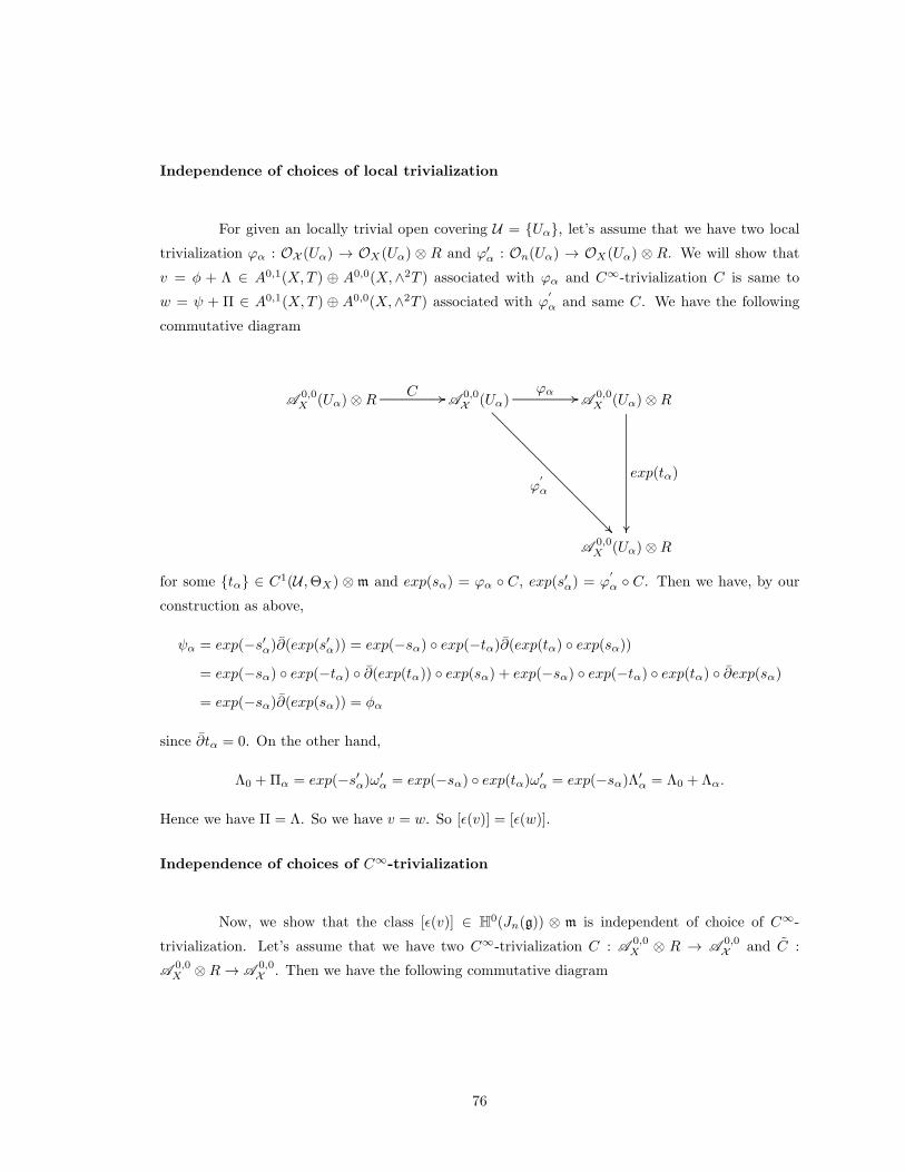
Independence of choices of local trivialization

For given an locally trivial open covering U = Uα, let’s assume that we have two local

trivialization ϕα : OX (Uα) → OX(Uα) ⊗ R and ϕ′α : On(Uα) → OX(Uα) ⊗ R. We will show that

v = φ + Λ ∈ A0,1(X,T ) ⊕ A0,0(X,∧2T ) associated with ϕα and C∞-trivialization C is same to

w = ψ + Π ∈ A0,1(X,T ) ⊕ A0,0(X,∧2T ) associated with ϕ′

α and same C. We have the following

commutative diagram

A0,0X (Uα)⊗R A

0,0X (Uα) A

0,0X (Uα)⊗R

A0,0X (Uα)⊗R

........................................................................................................................... ............C

........................................................................................................................... ............

ϕα

........................................................................................................................................................................................................................................................................................................... ............

ϕ′

α

.................................................................................................................................................................................................................................

exp(tα)

for some tα ∈ C1(U ,ΘX) ⊗ m and exp(sα) = ϕα C, exp(s′α) = ϕ′

α C. Then we have, by our

construction as above,

ψα = exp(−s′α)∂(exp(s′α)) = exp(−sα) exp(−tα)∂(exp(tα) exp(sα))

= exp(−sα) exp(−tα) ∂(exp(tα)) exp(sα) + exp(−sα) exp(−tα) exp(tα) ∂exp(sα)

= exp(−sα)∂(exp(sα)) = φα

since ∂tα = 0. On the other hand,

Λ0 +Πα = exp(−s′α)ω′α = exp(−sα) exp(tα)ω

′α = exp(−sα)Λ

′α = Λ0 + Λα.

Hence we have Π = Λ. So we have v = w. So [ǫ(v)] = [ǫ(w)].

Independence of choices of C∞-trivialization

Now, we show that the class [ǫ(v)] ∈ H0(Jn(g)) ⊗ m is independent of choice of C∞-

trivialization. Let’s assume that we have two C∞-trivialization C : A0,0X ⊗ R → A

0,0X and C :

A0,0X ⊗R→ A

0,0X . Then we have the following commutative diagram

76

A0,0X (X)⊗R A

0,0X (X)

A0,0X (X)⊗R

...................................................................................................................................................................................................................................... ............C

................................................................................................................................................................................................. ............

exp(u) = C−1 C

......................................................................................................................................................................................................

C

C−1 C is a homomorphism inducing identity up to m. As in the proof of Lemma 5.19, we can show

that there is an element u ∈ A0,0(T )⊗m such that C−1 C = exp(u).

For given an locally trivial open covering Uα and local trivializations ϕα : OX (Uα) →

OX(Uα)⊗R, let v = φ+ Λ be the element of (A0,1(X,T )⊕A0,0(X,∧2T ))⊗m induced from C and

v = φ + Λ be the element of (A0,1(X,T ) ⊕ A0,0(X,∧2T )) ⊗ m induced from C. We want to show

that [ǫ(v1)] = [ǫ(v0)].

Since exp(sα) = ϕα C, we have exp(sα) exp(u) = ϕα C. Hence we have

φ = [exp(sα) exp(u)]−1∂(exp(sα) exp(u))

= exp(−u) exp(−sα)∂exp(sα)exp(u) + exp(−u) exp(−sα)exp(sα)∂exp(u)

= exp(−u)∂exp(u) + exp(−u)φexp(u)

Λ0 + Λ = exp(−u) exp(−sα)(Λ′α)

= exp(−u)(Λ0 + Λ)

We set for t ∈ [0, 1] ⊂ R,

φt = exp(−tu)∂exp(tu) + exp(−tu)φexp(tu)

Λt = exp(−tu)(Λ0 + Λ)− Λ0

Note that φ0 = φ,Λ0 = Λ and φ1 = φ,Λ1 = Λ. We would like to show that [ǫ(v)] = [ǫ(φ + Λ)] =

[ǫ(φ + Λ)] = [ǫ(v)] by showing that [ǫ(vt)] := [ǫ(φt + Λt)] is constant independent of t. To this

end, we note that since the operator L = ∂ + [Λ0,−] is elliptic, H0(Jn(g)) is finite dimensional

vector space over C. Since g is a global section of a complex vector bundle over X , g is endowed

with a suitable metric, which induces a metric on H0(Jn(g)) by hodge theory which coincides with

the standard Euclidean topology and likewise for H0(Jn(g)) ⊗ m. So differentiation of a function

R→ H0(Jn(g))⊗m makes sense if the derivative exists with respect to the metric on H0(Jn(g))⊗m.

Now we claim that ddt ([ǫ(vt)]) =

ddt [(ǫ(φt + Λt)] = [ ddt(ǫ(φt + Λt))] = 0, which implies that [ǫ(vt)] is

constant, and so [ǫ(v)] = [ǫ(v)]. We note that

77

φ′t :=d

dt(φt) = −uexp(−tu)∂(exp(tu)) + exp(−tu)∂(exp(tu)u)

− uexp(−tu)φexp(tu) + exp(−tu)φexp(tu)u

= −uexp(−tu)∂(exp(tu)) + exp(−tu)∂(exp(tu))u + ∂u

− uexp(−tu)φexp(tu) + exp(−tu)φexp(tu)u

= −uφt + φtu+ ∂u = ∂u− [u, φt]

(Λt)′ :=d

dt(Λt) = −uexp(−tu)(Λ0 + Λ) = −u(Λt + Λ0)

= −[u,Λt] + [Λ0, u]

So v′t :=ddtvt =

ddt (φt + Λt) = φ′t + (Λt)′ = Lu− [u, φt + Λt] = Lu− [u, vt]. And we have

d

dt(ǫ(vt)) = (v′t, v

′t ⊙ vt, ...,

1

(n− 1)!v′t ⊙ vt ⊙ · · · ⊙ vt︸ ︷︷ ︸

n−1

) ∈ ⊕ni=1symig1 ⊗m

which corresponds to

(v′t, · · · , (−1)(i−1)i

21

(i− 1)!v′t ∧ vt ∧ · · · ∧ vt︸ ︷︷ ︸

i−1

, · · · , (−1)(n−1)n

21

(n− 1)!v′t ∧ vt ∧ · · · ∧ vt︸ ︷︷ ︸

n−1

)

in∧g.

Note that Lvt = −12 [vt, vt].

2 Let

(−u,−u⊙ αt, ...,1

(n− 1)!(−u)⊙ αt ⊙ ...⊙ αt

︸ ︷︷ ︸

n−1

) ∈n−1⊕

i=1

g0 ⊗ symig1 ⊗m

which corresponds to

(−u, · · · , (−1)(i−1)i

21

i!(−u) ∧ αt ∧ · · · ∧ αt

︸ ︷︷ ︸

i

, · · · , (−1)(n−2)(n−1)

21

(n− 1)!(−u) ∧ αt ∧ · · · ∧ αt

︸ ︷︷ ︸

n−1

)

in∧g.

We claim that this is the coboundary of ddt(ǫ(vt)). Indeed, (note that deg(u) = 0 and

2For given the locally trivial open covering Uα and local trivialization ϕα : OX (Uα) → OX(Uα) ⊗ R, let

Ct : A0,0X

⊗ R → A0,0X

be C∞-trivialization defined by Ct = C exp(tu). Then we have ϕα C = exp(sα) exp(tu).Then we have

φt = (exp(sα) exp(tu))−1∂(exp(sα) exp(tu))

Λ0 +Λt = (exp(sα) exp(tu))−1Λ′α

Hence by the construction, we have Lvt +12[vt, vt] = 0.

78

deg(vt) = 1.)

(−1)i+1L((−1)(i−1)i

21

i!(−u) ∧ vt ∧ · · · ∧ vt

︸ ︷︷ ︸

i

) + (−1)i(i+1)

2i+ 1

(i+ 1)![−u, vt] ∧ vt ∧ · · · ∧ vt

︸ ︷︷ ︸

i

+ (−1)i(i+1)

21

(i+ 1)!

(i+ 1

2

)

[vt, vt] ∧ (−u) ∧ vt ∧ · · · ∧ vt︸ ︷︷ ︸

i−1

= (−1)i(i+1)

21

i!(Lu ∧ vt ∧ · · · ∧ vt

︸ ︷︷ ︸

i

+u ∧ Lvt ∧ vt ∧ · · · ∧ vt − u ∧ vt ∧ Lvt ∧ vt ∧ · · · ∧ vt + · · ·

+ (−1)i−1u ∧ vt ∧ · · · ∧ vt︸ ︷︷ ︸

i−1

∧Lvt)− (−1)i(i+1)

21

i![u, vt] ∧ vt ∧ · · · ∧ vt

︸ ︷︷ ︸

i

+ (−1)i(i+1)

21

(i− 1)!

1

2u ∧ [vt, vt] ∧ vt ∧ · · · ∧ vt

︸ ︷︷ ︸

i−1

= (−1)i(i+1)

2 (1

i!Lu ∧ vt ∧ · · · ∧ vt

︸ ︷︷ ︸

i

+1

(i− 1)!u ∧ Lvt ∧ vt ∧ · · · ∧ vt

︸ ︷︷ ︸

i−1

−1

i![u, vt] ∧ vt ∧ · · · ∧ vt

︸ ︷︷ ︸

i

)

+ (−1)i(i+1)

21

(i− 1)!

1

2u ∧ [vt, vt] ∧ vt ∧ · · · ∧ vt

︸ ︷︷ ︸

i−1

= (−1)i(i+1)

21

i!(Lu− [u, vt]) ∧ vt ∧ · · · ∧ vt

︸ ︷︷ ︸

i−1

= (−1)i(i+1)

21

i!v′t ∧ vt ∧ · · · ∧ vt︸ ︷︷ ︸

i

.

So we have [ ddt (ǫ(vt))] = 0.

In conclusion, for given an infinitesimal Poisson deformation X of (X,Λ0), we can canon-

ically associate the Poisson deformation X up to equivalence with the cohomology class [ǫ(v)]. In

the next chapter, we will show that under the assumption HP 1(X,Λ0) = 0, for given a choice

v, w ∈ (A0,1(X,T ) ⊕ A0,0(X,∧2T )) ⊗ m with [ǫ(v)] = [ǫ(w)], the Poisson deformation associated

with v is equivalent to the Poisson deformation associated with w.

79

Chapter 6

Universal Poisson deformations

6.1 Isomorphism of two deformation functors Defg ∼= PDef(X,Λ0)

In this section, we will show that two functors of Artin rings are isomorphic: namely the

Poisson deformation functor Def(X,Λ0) is isomorphic to the deformation functor Defg associated

to the differential graded Lie algebra g = (⊕

p+q−1=i,q≥1 A0,p(X,∧qT ), L = ∂ + [Λ0,−], [−,−]).

So this shows that deformations of a compact holomorphic Poisson manifold are controlled by the

differential graded Lie algebra g. For deformation functors associated with a differential graded Lie

algebra, we refer to [Man04].

6.1.1 Deformation functors

Definition 6.1 A functor of Artin rings is a covariant functor

F : Art→ Sets

such that F (C) has only one element, where Art is the category of local artinian C-algebra with

residue C, and Sets is the category of sets.

Definition 6.2 (functors associated with a DGLA L) Let L = (⊕

i≥0 Li, d, [−,−]) be a dif-

ferential graded Lie algebra and (R,m) ∈ Art. Let MC(L)(R) be the set of all Maurer-Cartan

elements of L⊗m, i.e

MCL(R) = x ∈ L1 ⊗m|dx+1

2[x, x] = 0

Then MCL : Art→ Sets is a functor.

Let g = L⊗m be the induced differential graded Lie algebra from L. Then g0 = L0⊗m is a

nilpotent Lie algebra. Then the set exp(g0) = ex|x ∈ g0 forms a group by the Campbell-Hausdorff

80

formula. We have a group action of exp(g0) on g1 = L1 ⊗m given by

ea · x := x+∑

n≥1

(ad a)n−1

n!([a, x]− da) where ad a : g1 → g1 defined by b 7→ [a, b]

The action is known as the gauge action of exp(g0) on g1 and the set of Maurer-Cartan elements is

stable under the gauge action.

Definition 6.3 Let x, y ∈ MCL(R). We say that x is gauge equivalent to y if there exists ea ∈

exp(g0) such that ea · x = y. Let DefL(R) be the set of all gauge equivalence classes of elements of

MCL(R). Then the functor DefL : Art→ Sets is called the deformation functor associated to the

differential graded Lie algebra L.

Definition 6.4 We say that a functor of Artin rings F is controlled by a differential graded Lie

algebra L if F ∼= DefL.

Definition 6.5 (Poisson deformation functor) Let (X,Λ0) be a compact holomorphic Poisson

manifold. The Poisson deformation functor Def(X,Λ0) : Art→ Sets is defined by

PDef(X,Λ0)(R) = equivalent classes of infinitesimal Poisson deformations of (X,Λ0) over R

In the next subsection, we will prove that Defg ∼= PDef(X,Λ0).

6.1.2 The Poisson deformation functor Def(X,Λ0) is controlled by the dif-

ferential graded Lie algebra g = (⊕

p+q−1=i,q≥1A0,p(X,∧qT ), L = ∂ +

[Λ0,−], [−,−])

Let X → SpecR be an infinitesimal Poisson deformation of (X,Λ0), where (R,m) is gen-

erated by < 1,m1, ...,mr > with exponent n. Let Uα be a locally trivial open cover of X . We

defined a sheaf A 0,p(∧qTX/R), a bracket [−,−] and the deaulbault differential ∂X . For q = 0, we

will denote this sheaf by A0,pX and similarly for A

0,pX .

Given an element v := φ+ Λ ∈ (A0,1(X,T )⊕A0,0(X,∧2T ))⊗m with L(φ+ Λ) = − 12 [φ+

Λ, φ + Λ]. In particular, we have ∂φ = − 12 [φ, φ]. We define an operator ∂ + φ := ∂ ⊗ 1 + φ on

A 0,p ⊗R and a sequence

0→ A0,0X ⊗R

∂+φ−−−→ A

0,1X ⊗R

∂+φ−−−→ · · ·

∂+φ−−−→ A

0,pX ⊗R

∂+φ−−−→ (6.6)

which is a complex by the condition ∂φ = − 12 [φ, φ]. By tensoring ⊗RR/m, we have

0→ A0,0X ⊗ C

∂−→ A

0,1X ⊗ C

∂−→ · · ·

81

which is a acyclic resolution of OX . Hence the complex (6.6) is exact in positive degree.

We define

O(v) := ker(∂ + φ : A0,0X ⊗R→ A

0,1X ⊗R)

which is a flat R-sheaf on X .1 O(v) has a Poisson bracket induced by Λ0 +Λ. We define on −,−

on O(v) by

f, g := [[Λ0 + Λ, f ], g]

for local sections f, g ∈ O(v). Then −,− defines a biderivation since d(gh) = gdh + hdg and R-

bilinear since for a = a0 + a1m1 + · · · armr ∈ R where ai ∈ C, we have da = 0. [Λ0 +Λ,Λ0 +Λ] = 0

shows that −,− satisfies the Jacobi identity. So it remains to show that O(v) is closed under

−,−. Note that for f, g ∈ O(v), we have ∂f + [φ, f ] = 0, ∂g + [φ, g] = 0. We set ω = Λ0 + Λ.

Then we have ∂ω + [φ, ω] = 0

∂[[ω, f ], g] + [φ, [[ω, f ], g]] = [∂[ω, f ], g] + [[ω, f ], ∂g] + [[φ, [ω, f ]], g] + [[ω, f ], [φ, g]]

= [[∂ω, f ], g]− [[ω, ∂f ], g] + [[[φ, ω], f ], g]− [[ω, [φ, f ]], g]

= 0

So we have f, g ∈ O(v). Hence O(v) is a sheaf of PoissonR-algebras. We also haveO(v)⊗RR/m ∼=

OX as Poisson sheaves over C. So O(v) defines an infinitesimal Poisson deformation of (X,Λ0) over

R.

Now we define the map

O : Defg(R)→ PDef(X,Λ0)(R)

v = φ+ Λ 7→ O(v)

We claim that v is gauge equivalent to w if and only if O(v) ∼= O(w) as Poisson R-sheaves.

This claim shows that the map O is well-defined and injective. Let v = φ + Λ, w = ψ + Π ∈

(A0,1(X,T )⊕A0,0(X,∧2T ))⊗m. Since v is gauge equivalent to w, for some a ∈ A0,0(X,T )⊗m, we

have

(1)ψ = φ+∑

n≥1

(ad a)n−1

n!([a, φ]− ∂a)

(2)Π = Λ +∑

n≥1

(ad a)n−1

n!([a,Λ]− [Λ0, a]) = exp(a)(Λ0 + Λ)− Λ0

(1) is equivalent that the following commutative diagram commutes:

1In general, let R be an artinian local ring with residue field k and M be an R-module. Let

M → N0 → N1 → · · ·

be a flat resolution such that this induces a resolution

M ⊗ k → N0 ⊗ k → N1 ⊗ k · · ·

Then M is a R-flat.

82

A0,0X ⊗R

∂+φ−−−−→ A

0,1X ⊗R

exp(a)

y

yexp(a)

A0,0X ⊗R

∂+φ′

−−−−→ A0,1X ⊗R

which implies O(v) ∼= O(w) as sheaves of R-algebras.

(2) means Λ0 + Π = exp(a)(Λ0 + Λ) which means O(v) ∼= O(w) as sheaves of Poisson

R-algebras. So we get the claim.

Now we show that O : Defg(R) → Def(X,Λ0)(R) is surjective. For given an infinitesimal

Poisson deformation of (X,Λ0) over (R,m), we showed that there is a canonically associated element

v = φ+ Λ ∈ (A0,1(X,T )⊕A0,0(X,∧2T ))⊗ m with L(φ+ Λ) + 12 [φ + Λ, φ+ Λ] = 0. We claim that

for each α, the following diagram is commutative.

A0,0X (Uα)⊗R

∂+φ−−−−→ A

0,1X (Uα)⊗R

exp(sα)

y

yexp(sα)

A0,0X (Uα)⊗R

∂X=∂−−−−→ A

0,1X (Uα)⊗R

Note that exp(sα) = ϕα C. Indeed, the commutativity means that

∂f + φ(f) = ∂f + exp(−sα) ∂(exp(sα))f

= ∂f + exp(−sα) (∂ exp(sα)− exp(sα) ∂)f

= exp(−sα) ∂ exp(sα)f

Since the diagram is compatible with each α, we have the following commutative diagram

of sheaves

A0,0X ⊗R

∂+φ−−−−→ A

0,1X ⊗R

∼=

y

y∼=

A0,0X

∂X−−−−→ A0,1X

So we have isomorphism of sheaves

O(v) := ker(∂ + φ : A0,0X ⊗R→ A

0,1X ⊗R) ∼= OX = ker(∂X : A0,0

X → A0,1X )

O(v) is a sheaf of Poisson R-algebras as above defined by

f, g := [[Λ0 + Λ, f ], g] for local sections f, g ∈ O(v)

Now we claim that as Poisson R-sheaves, we have

O(v) ∼= OX

83

We check this locally on Uα: for f, g ∈ Γ(Uα,O(v)) = ker(∂ + φ : A0,0X (Uα)⊗R→ A

0,1X (Uα)⊗R),

exp(sα)f, g = exp(sα)[[Λ0 + Λ, f ], g] = exp(sα)[[Λ′′α, f ], g] = [[exp(sα)Λ

′′α, exp(sα)f ], exp(sα)g]

= [[exp(sα)exp(−sα)Λ′α, exp(sα)f ], exp(sα)g] = [[Λ′

α, exp(sα)f ], exp(sα)g]

where Λ′α ∈ Γ(Uα,A

0,0(∧2TX)) ⊗ R is the Poisson structure on OX(Uα) ⊗ R ∼= OX (Uα) and

Λ′′α = exp(−sα)Λ′

α. (See Remark 5.24 for notations)

Hence the infinitesimal Poisson deformation X of (X,Λ0) over R is equivalent to O(v) :=

ker(∂ + φ : A0,0X ⊗ R → A

0,1X ⊗ R) equipped with the Poisson structure Λ0 + Λ. This shows that

the map O : Defg(R)→ Def(X,Λ0)(R) is surjective.

So we proved that for an artinian local C-algebra R with residue C, we have an isomorphism

O : MCg(R) → PDef(X,Λ0)(R). To show that Defg ∼= PDef(x,Λ0), we have to show that O is a

morphism of functors of Artin rings, in other words, O is compatible with any local homomorphism

R→ S in Art.

Definition 6.7 (Base change) Given an infinitesimal Poisson deformation X of (X,Λ) over R,

and a local C-algebra homomorphism (R,mR) → (S,mS), we can define an infinitesimal Poisson

deformation X ×SpecR Spec S of (X,Λ) over S by base change.

X −−−−→ X ×SpecR Spec S −−−−→ Xy

y

y

SpecC −−−−→ Spec S −−−−→ SpecR

We only need to explain the induced Poisson structure of XS := X ×Spec R Spec S over S. For any

open set U of X, OXS (U) = OX (U)⊗R S. We define the Poisson bracket −,−S on OXS (U) by

f ⊗ s1, g ⊗ s2S = f, gR ⊗ s1s2

where −,−R is the Poisson bracket on OX (U).

We note that the induced infinitesimal Poisson deformation by the base change (R,mR)→

(S,mS) can be interpreted in terms of a Mauer-Cartan element of X . Let φ + Λ ∈ (A0,1(X,T ) ⊕

A0,0(X,∧2T )) ⊗ mR be a Mauer Cartan element of X . Hence OX is equivalent to ker(∂ + φ :

A 0,0⊗R→ A 0,1⊗R) with the Poisson structure Λ0+Λ. The homomorphism g : (R,mR)→ (S,mS)

induces the homomorphisms A0,p(X,∧qT )⊗mR → A0,p(X,∧qT )⊗mS. Let φS+ΛS be the image of

φ+Λ, which also satisfy LS(φS+ΛS)+12 [φS+ΛS, φS+ΛS] = 0. We have the following commutative

diagram

(A 0,0X ⊗R,Λ0 + ΛR)

∂+φ−−−−→ A

0,1X ⊗R

y

y

(A 0,0X ⊗ S,Λ0 + ΛS)

∂+φS−−−−→ A

0,1X ⊗ S

84

We claim that

Proposition 6.8 OXS is equivalent to (φS + ΛS).

Proof. We recall that for given locally trivial open covering Uα, and local trivialization ϕα :

OX (Uα) → OX(Uα) ⊗ R and C∞-trivialization C : A0,0X ⊗ R → A

0,0X for the family X , we have

φ = exp(−sα)∂exp(sα) ∈ A0,1(X,T )⊗mR and Λ = exp(−sα)(Λ0 +Λα)−Λ0 ∈ A0,0(X,∧2T )⊗mR.

Now we consider the family XS over S. For the same open covering Uα, the local trivialization is

induced from ψα by tensoring ⊗RS and C∞ trivialization is also induced from C by tensoring ⊗RS.

This observation gives the proposition.

Hence we have the following commutative diagram

Defg(R)O

−−−−→ PDef(X,Λ0)(R)y

y

Defg(S)O

−−−−→ PDef(X,Λ0)(S)

Hence we proved the following theorem.

Theorem 6.9 Let (X,Λ0) be a compact holomorphic Poisson manifold. Then the Poisson defor-

mation functor Def(X,Λ0) is controlled by the differential graded Lie algebra g = (⊕

p+q−1=i,p≥1,q≥1

A0,p(X,∧qT ), L = ∂ + [Λ0,−], [−,−]). In other words, we have an isomorphism of two functors

Defg ∼= PDef(X,Λ0)

6.2 Universal Poisson deformations

Now we assume that for a holomorphic Poisson manifold (X,Λ0), HP1(X,Λ0) = 0.

6.2.1 Independence of choices of morphic elements giving the same co-

homology class

Let m be the maximal ideal of a local artinian C-algebraR with residue such that mn+1 = 0.

Our goal is that for given v = φ+Λ, w = ψ+Π ∈ g1⊗m such that [ǫ(v)] = [ǫ(w)] in H0(Jn(g))⊗m,

where ǫ(v) = (v, 12 v⊙ v, ...,1n! v ⊙ · · · ⊙ v︸ ︷︷ ︸

n

) ∼=dec (v, · · · , (−1)(n−1)n

21n! v ∧ · · · ∧ v︸ ︷︷ ︸

n

) ∈⊕n

i=1 symig1⊗mi

and Lv = − 12 [v, v], and same for w, we want to show that the Poisson deformation O(v) is equivalent

to the Poisson deformation O(w). In other words, we want to show that

1. there exists u0 ∈ g0 ⊗m such that exp(u0)(∂ + φ)exp(−u0) = ∂ + ψ.

85

A0,0X ⊗R

∂+φ−−−−→ A

0,1X ⊗R

exp(u0)

y

yexp(u0)

A0,0X ⊗R

∂+ψ−−−−→ A

0,1X ⊗R

2. exp(u0)(Λ0 + Λ) = Λ0 +Π

We will prove the statement by induction on the exponent k of maximal ideal of artinian

local C-algebra with residue C. Let k = 1. So we have m2 = 0. Let [ǫ(v)] = [ǫ(w)] ∈ H0(J1(g))⊗m.

Then there exists u0 ∈ g0⊗m such that (−1)1Lu0 = w−v. So we have Lu0 = ∂u0+[Λ0, u0] = v−w.

In other words,

∂u0 = φ− ψ

[Λ0, u0] = Λ−Π

We note that exp(u0) = 1+u0 and exp(−u0) = 1−u0. Then since u0 ∈ g0⊗m, φ, ψ,Λ,Π ∈

g1 ⊗m and m2 = 0, we have

1.

exp(u0)(∂ + φ)exp(−u0) = (1 + u0)(∂ + φ)(1 − u0) = (∂ + φ+ u0∂ + u0φ)(1 − u0)

= ∂ + φ+ u0∂ + u0φ− ∂ · u0 − φu0 − u0∂ · u0 − u0φu0

= ∂ + φ+ u0∂ − ∂ · u0 = ∂ + φ− ∂u0

= ∂ + ψ

2.

exp(u0)(Λ0 + Λ) = (1 + u0)(Λ0 + Λ) = Λ0 + Λ+ [u0,Λ0 + Λ]

= Λ0 + Λ− [Λ0, u0] = Λ0 + Λ− (Λ−Π)

= Λ0 +Π

So the statement holds for k = 1.

Now let’s assume that the statement holds for k = n−1. Now let (R,m) be a local artinian

C-algebra with exponent n and let [ǫ(v)] = [ǫ(w)] ∈ H0(Jn(g)) ⊗ m where v, w ∈ g1 ⊗ m. We have

the following exact sequence of finite dimensional vector spaces

0→ mn → R→ R/mn → 0

So we have the following splitting as vector spaces

R ∼= (R/mn)⊕mn

86

Note that (R/mn,m/mn) is a local artinian C-algebra with exponent n − 1. Now let

v = v1+v2 = (φ1+Λ1)+(φ2+Λ2) and w = w1+w2 = (ψ1+Π1)+(ψ2+Π2), where v1, w1 ∈ g1⊗(R/mn)

and v2, w2 ∈ mn. Then we have [ǫ(v1)] = [ǫ(w1)] ∈ H0(Jn−1(g))⊗m/mn, where v1, w1 ∈ g1⊗m/mn.

By the induction hypothesis,

1. we have the following commutative diagram.

A0,0X ⊗R/mn

∂+φ1−−−−→ A

0,1X ⊗R/mn

exp(u)

y

yexp(u)

A0,0X ⊗R/mn

∂+ψ1−−−−→ A

0,1X ⊗R/mn

where some u ∈ g0 ⊗m/mn.

2. exp(u)(Λ0 + Λ1) = Λ0 +Π1.

Let’s consider the natural projection g0 ⊗ R ∼= g0 ⊗ (R/mn ⊕ mn) → g0 ⊗ R/mn. Choose

the lifting of u to be u+ 0 ∈ g0 ⊗ (R/mn ⊕mn) ∼= g0 ⊗R. Then

1. we have the following commutative diagram.

A0,0X ⊗R

∂+φ1+φ2−−−−−−→ A

0,1X ⊗R

exp(u+0)

y

yexp(u+0)

A0,0X ⊗R

∂+ψ1+φ2−−−−−−→ A

0,1X ⊗R

since φ2 = φ2 exp(u) = exp(u) φ2. (note that φ2 ∈ A0,1(X,T ) ⊗ mn, u ∈ g0 ⊗ m and

mn+1 = 0.)

2. exp(u)(Λ0+Λ1+Λ2) = Λ0+Π1+Λ2 since exp(u)(Λ2) = Λ2 (note that Λ2 ∈ A0,0(X,∧2T )⊗mn).

Since O(v1 + v2) and O(w1 + v2) are equivalent Poisson deformations, we have [ǫ(v1 + v2)] =

[ǫ(w1 + v2)]. If we show that O(w1 + v2) is equivalent to O(w1 + w2), then this means that O(v) is

equivalent to O(w).

Since [ǫ(w1 + v2)] = [ǫ(w1 + w2)], there exists (u0, ..., un−1) ∈⊕n−1

i=0 g0 ⊗ symig1 ⊗ mi+1

such that

u0(−1)1L−−−−−−−→ w2 − v2

δ

x

u1(−1)2L−−−−−−−→ − 1

2((w1 + w2)2 − (w1 + v2)2) = 0

δ

x

· · · −−−−−−−→ · · ·

δx

un−1(−1)nL−−−−−−−→ (−1)

(n−1)n2 1

n!((w1 + w2)n − (w1 + v2)n) = 0

87

Since v2, w2 ∈ g1 ⊗mn and w1 ∈ g1 ⊗m, we have

(−1)(i−1)i

21

i!((w1 + w2)

i − (w1 + v2)i) = 0 for i > 1.

Let’s consider un−1 ∈ g0⊗symn−1g1⊗mn. Write un−1 =∑

k ak⊗bk where ak ∈ g0 and bk are linearly

independent in symn−1g1 ⊗mn. Then since (−1)nLun−1 = 0, we have∑

k Lak ⊗ bk + ak ⊗ Lbk=0.

So Lak = 0. Since bk are linearly independent and, Lak ⊗ bk and ak ⊗ Lbk live in different spaces,

we have Lak = 0. Since H0(g) = HP 1(X,Λ0) = 0, we have ak = 0. un−1 = 0. In this way we can

show that u1 = ... = un−1 = 0. Hence we have (−1)1Lu0 = w2 − v2 ∈ g1 ⊗ mn. So Lu0 = v2 − w2.

In other words, we have

∂u0 = φ2 − ψ2

[Λ0, u0] = Λ2 −Π2

Let u0 := x1 + x2 ∈ g0⊗R ∼= g0⊗ (R/mn⊕mn). Since Lx1 = 0 and Lx2 = v2−w2, we have x1 = 0

by H0(g) = 0. So u0 ∈ g0 ⊗mn. Then we have the following commutative diagram.

A0,0X ⊗R

∂+ψ1+φ2−−−−−−→ A

0,1X ⊗R

exp(u0)

y

yexp(u0)

A0,0X ⊗R

∂+ψ1+ψ2−−−−−−→ A

0,1X ⊗R

Indeed,

exp(u0)(∂ + ψ1 + φ2)exp(−u0) = (1 + u0)(∂ + ψ1 + φ2)(1− u0)

= ∂ + ψ1 + φ2 + u0∂ − ∂u0

= ∂ + ψ1 + φ2 − ∂u0

= ∂ + ψ1 + ψ2

And

exp(u0)(Λ0 +Π1 + Λ2) = (1 + u0)(Λ0 +Π1 + Λ2)

= Λ0 +Π1 + Λ2 + [u0,Λ0] = Λ0 +Π1 + Λ2 − [Λ0, u0]

= Λ0 +Π1 +Π2

So the induction holds for k = n.

6.2.2 n-th Universal Poisson deformations

Recall that Run = C⊕ mun := C⊕ H0(Jn(g))∗ is a local artinian C-algebra with residue C

and expoent n (i.e. mun+1n = 0).

88

Definition 6.10 (n-th universal Poisson deformation) Since the identity map H∗(Jn(g)) →

H∗(Jn(g)) is a homomorphism, it corresponds to a morphic element

[ǫ(vu)] = [(vu,1

2vu ⊙ vu, ....,

1

n!vu ⊙ · · · ⊙ vu︸ ︷︷ ︸

n

)] ∈ H0(Jn(g))⊗mun

where vu := φu + Λu ∈ g1 ⊗ H0(Jn(g))∗. Then vu defines an infinitesimal Poisson deformaiton

Pun := O(vu) over a local artinian C-algebra Run := C⊕H0(Jn(g))∗. We will call Pun be a n-th order

universial Poisson deformation of (X,Λ0) over Run.

Let P be an infinitesimal Poisson deformation of (X,Λ0) over (R,m) with mn+1 = 0. Assume that

HP 1(X,Λ0) = 0. Let v = φ + Λ be an Maurer Cartan element corresponding to the infinitesimal

Poisson deformation P of (X,Λ0) over R. Then [ǫ(v)] = [(v, 12 v⊙v, ...,1n! v⊙· · ·⊙v)] ∈ H0(Jn(g))⊗m,

which induces a homomorphism [ǫ(v)] : mun = H0(Jn(g))∗ → m. Via the morphism r := [ǫ(v)],

vu ∈ g1 ⊗ mun is sent to vu ∈ g1 ⊗ m. Then vu satisfies the Maurer Cartan equation since vu

does. Hence [ǫ(vu)] ∈ H0(Jn(g)) ⊗ m defines a morphic element and we have the corresponding

homomorphism [ǫ(vu)] : H0(Jn(g))∗ id=[ǫ(vu)]−−−−−−→ H0(Jn(g))

∗ r−→ m, which is exactly [ǫ(v)]. Hence

we have [ǫ(v)] = [ǫ(vu)]. Hence by the assumption of HP 1(X,Λ0) = 0, the induced deformation

vu = φu + Λu from the deformation vu by the base change [ǫ(v)] : H0(Jn(g))∗ → m

(A 0,0X ⊗Run,Λ0 + Λu)

∂+φu−−−−→ A

0,1X ⊗Run

y

y

(A 0,0X ⊗R,Λ0 + Λu)

∂+φu−−−−→ A

0,1X ⊗R

is equivalent to v = φ+Λ, which represents the infinitesimal Poisson deformation P of (X,Λ0) over

R. Then we have P/R ∼= r∗Pun = Pun ×Spec(Run)Spec(R). This proves our main Theorem 11 (2) in

the Introduction of the part II of the thesis.

6.2.3 Formal Completition

The natural map H0(Jn−1(g))→ H0(Jn(g)) gives dually the homomorphism H0(Jn(g))∗ →

H0(Jn−1(g))∗. Set mun = H0(Jn(g))

∗ and Run := C ⊕ mun. Take the inverse limit mu := lim←−n

mun.

Then we have

Ru := C⊕mu = C⊕ lim←−n

mun = lim←−n

(C⊕mun) = lim←−n

Run

By our construction of Jn(g), we have C ⊕ mu/mun+1 = C ⊕ mun. Hence (Ru,mu) =

lim←−

(Run,mun) is a complete local noetherian C-algebra with respect to the mu-adic topology.

89

From mun = H0(Jn(g))∗ → mun−1 = H0(Jn−1(g))

∗, the morphic element [ǫ(vu = φu+Λu)] =

[(vu,12 vu⊙ vu, · · · ,

1n! vu⊙· · ·⊙ vu)] ∈ H0(Jn(g))⊗mun inducing the identity map on H0(Jn(g))

∗, gives

a morphic element [ǫ(vu = φu + Λu)] = [(¯vu, · · · ,1

(n−1)!¯vu ⊙ · · · ⊙ ¯vu, 0)] ∈ H0(Jn(g)) ⊗ mun−1 (via

mun → mun−1) which can be considered as an element in H0(Jn−1(g)) ⊗ mun−1 inducing the identity

map on H0(Jn−1(g))∗ and so we have the following commutative diagram:

H0(Jn(g))∗ id=[ǫ(vu)]−−−−−−→ H0(Jn(g))

∗

y

y

H0(Jn−1(g))∗ id=[ǫ(vu)]−−−−−−→ H0(Jn−1(g))

∗

Hence we have the following commutative diagram

(A 0,0X ⊗Run,Λ0 + Λu)

∂+φu−−−−→ A

0,1X ⊗Run

y

y

(A 0,0X ⊗Run−1,Λ0 + Λu))

∂+φu−−−−→ A

0,1X ⊗Run−1

So n-th universal Poisson deformations Pun /Run fit together to form a direct system with

limit

Pu/Ru = lim−→

Pun /Run

Now we set R = lim←−

(Rn,mn) is a complete local noetherian C-algebra where (Rn,mn) is a

local artinian C-algebra with residue C and P /R = lim−→n

Pn/Rn is a formal Poisson analytic space

over R, where Pn/Rn is an infinitesimal Poisson deformation of (X,Λ0), which can be interpreted

as a sequence rn of morphic elements where rn ∈ H0(Jn(g)) ⊗ mn such that rn induces rn−1 ∈

H0(Jn−1(g)) ⊗ mn−1 by the natural map mn → mn−1. Hence we have the following commutative

diagram:

H0(Jn(g))∗ rn−−−−→ mn

y

y

H0(Jn−1(g))∗ rn−1−−−−→ mn−1

So we have the map r = limnrn : Ru → R which induces P /R = r∗(Pu/Ru). This proves our main

Theorem 11 (3) in the Introduction of the part II of the thesis. So we complete the Theorem 11.

90

Part III

Deformations of algebraic Poisson

schemes

91

In the third part of the thesis, we study deformations of algebraic Poisson schemes over

an algebraic closed field k, which is an algebraic version of the first part of the thesis. In chapter

7, we discuss the definition of Poisson schemes, morphisms and cohomology. A Poisson scheme X

is a scheme whose structure sheaf OX is a sheaf of Poisson k-algebras. Equivalently, a Poisson

structure on a scheme X is characterized by an element Λ0 ∈ Γ(X,H omOX (∧2Ω1

OX/k,OX)) with

[Λ0,Λ0] = 0. By a deformation of a Poisson scheme (X,Λ0) we mean a commutative diagram

ξ :

(X,Λ0) −−−−→ (X ,Λ)y

yπ

Spec(k)s

−−−−→ S

where π is flat and surjective, and S is connected, (X ,Λ) is a Possoin scheme over S defined by

Λ ∈ Γ(X ,H om(∧2Ω1X/S,OX )) with X ∼= X ×S Spec(k) as a Poisson isomorphism. Note that when

we ignore Poisson structures, a Poisson deformation is an usual flat deformation of an algebraic

scheme X . By following Sernesi’s book [Ser06], we extend the formalism of ordinary flat deforma-

tions to Poisson deformations. We show that given a Poisson scheme (X,Λ0), first order Poisson

deformation (i.e Poisson deformations over a dual number k[ǫ]) whose underlying flat deformation

(when we ignore Poisson structures) is locally trivial, is naturally in one to one correspondence

with HP 2(X,Λ0) which is the second (truncated) Lichnerowicz-Poisson cohomology group, in other

words 2nd hypercohomology of the following complex of sheaves induced by [Λ0,−].

0→H omOX (Ω1X/k,OX)

[Λ0,−]−−−−→H omOX (∧

2Ω1X/k,OX)

[Λ0,−]−−−−→H omOX (∧

3Ω1X/k,OX)

[Λ0,−]−−−−→ · · ·

We also show that for a smooth Poisson algebraic scheme over k, any small extension e : 0 →

(t) → A → A → 0 (i.e (A,m), (A, m) are local artinian k-algebras with residue k and t · m = 0),

and an infinitesimal Poisson deformation ξ of (X,Λ0) over Spec(A), we can associate an element

oξ(e) ∈ HP 3(X,Λ0) such that oξ(e) is 0 if and only if a lifting of ξ to A exists. So HP 3(X,Λ0) is an

obstruction space. We also show that if HP 2(X,Λ0) = 0, then (X,Λ0) is rigid, which means that

any infinitesimal Poisson deformation of (X,Λ0) over A is trivial for all local artinian k-agebra A.

In chapter 8, we discuss Poisson deformation functor PDef(X,Λ0) which is a functor of

Artin rings. For a local artinian k-algebra A with residue k, PDef(X,Λ0)(A) is the set of Pois-

son deformations over Spec(A) up to Poisson equivalence. We show that for a smooth projective

Poisson scheme (X,Λ0), PDef(X,Λ0) satisfies Schlessinger’s criterion (H0), (H1), (H2), (H3) and so

PDef(X,Λ0) has a miniversal family. We also show that in addition if HP 1(X,Λ0) = 0, PDef(X,Λ0)

is pro-representable.

In chapter 9, we extend the construction of a cotangent complex ([LS67]) to Poisson cases.

Let A→ B be a Poisson homomorphism of Poisson k-algebras, and M be a Poisson B-module. We

construct PT i(B/A,M) in a similar way to construct T i(B/A,M) in [LS67]. As an application to

Poisson deformation, we show that for a Poisson algebra B0, PDefSpec(B0)(k[ǫ]) is a natural one

to one correspondence with PT 1(B0/k,B0). We also show that given a Poisson algebra B0 and an

92

Poisson ideal I of B0, deformations of a Poisson subscheme Spec(C) of Spec(B0) over Spec(k[ǫ]) is

one to one correspondence with PT 1(C/B0, C) where C = B0/I.

93

Chapter 7

Deformations of algebraic Poisson

schemes

7.1 Definitions of Poisson schemes, morphisms and cohomol-

ogy

In this section, every algebra is a commutative k-algebra, where k is a field. Our reference

is [LGPV13] Chapter 3. For algebraic geometry, we refer to [Har77], [Liu02].

7.1.1 Characterization of a Poisson bracket −,− of a Poisson algebra A

over R

In this subsection, we will characterize a Poisson structure of a commutative algebra A

over R in terms of an element Λ ∈ HomA(Ω1R/A, A) with [Λ,Λ] = 0 where [−,−] is the Schouten

bracket on⊕

p≥1HomA(∧pΩ1

A/R, A).

Definition 7.1 Let A be a commutative R-algebra and let p ≥ 1. A skew symmetric p-linear map

P ∈ HomR(∧pA,A) is called a skew symmetric p-derivation of A over R, if P is a derivation in

each of its components.

Let Ω1A/R be the A-module of relative kahler differential forms of A over R. Then the R-

module of all skew symmetric p-linear maps inHomR(∧p, A,A) is identified withHomA(∧pΩ1A/R, A).

Let P be a skew symmetric p linear map inHomR(∧pA,A). Then the associated P ∈ HomA(∧pΩ1A/R, A)

is defined in the following way: P (da1∧· · ·∧dap) := P (a1, · · · ap) where d : A→ Ω1A/R is the canonical

map.

94

The Shouten bracket on⊕

p≥1HomA(∧pΩ1A/R, A) and characterization of a Poisson bracket

on A

Definition 7.2 For p, q ∈ N, a (p, q)-shuffle is a permutation σ of the set 1, ..., p+ q, such that

σ(1) < · · · < σ(p) and σ(p+1) < · · · < σ(p+ q). The set of all (p, q)-shuffles is denoted by Sp,q. For

a shuffle σ ∈ Sp,q, we denote the signature of σ by sgn(σ). By convention, Sp,−1 := ∅ and S−1,q := ∅

for p, q ∈ N.

Definition 7.3 We define the Schouten bracket [−,−] on⊕

p≥1HomA(∧pΩ1A/R, A), namely a fam-

ily of maps

[−,−] : HomA(∧pΩ1

A/R, A)×HomA(∧qΩ1

A/R, A)→ HomA(∧p+q−1Ω1

A/R, A)

for p, q ∈ N in the following way: let P ∈ HomA(∧pΩ1A/R, A) and Q ∈ HomA(∧qΩ1

A/R, A), and for

F1, ..., Fp+q−1 ∈ A by

[P,Q](dF1 ∧ · · · ∧ dFp+q−1) =∑

σ∈Sq,p−1

sgn(σ)P (d(Q(dFσ(1) ∧ ... ∧ dFσ(q))) ∧ dFσ(q+1) · · · ∧ dFσ(q+p−1))

−(−1)(p−1)(q−1)∑

σ∈Sp,q−1

sgn(σ)Q(d(P (dFσ(1) ∧ ... ∧ dFσ(p))) ∧ dFσ(p+1) ∧ · · · ∧ dFσ(p+q−1))

Example 7.4 Let P ∈ HomA(∧2Ω1A/R, A) and Q ∈ HomA(Ω

1A/R, A). Then

[P,Q](dF1 ∧ dF2) = P (dQ(F1) ∧ dF2)− P (d(Q(F2)) ∧ dF1)−Q(d(P (dF1 ∧ dF2)))

Proposition 7.5 Let A be a commutative algebra over R. If Λ is a skew symmetric biderivation of

A over R, i.e Λ ∈ HomA(∧2Ω1A/R, A), then P defines a Poisson bracket (i.e Jaocbi identity holds)

if and only if [Λ,Λ] = 0.

Proof. See [LGPV13] Proposition 3.5 page 80.

Notation 13 Let A be a Poisson algebra over R with a Poisson bracket −,−. Let Λ be the

associated biderivation with the Poisson bracket −,−. Then we will denote by (A,Λ) the Poisson

algebra A over R with the Poisson bracket −,−.

Remark 7.6 Let (A,Λ) be a Poisson algebra over R with the Poisson structure Λ ∈ HomA(∧2,Ω1

A/R, A)

with [Λ,Λ] = 0. If we let g = ⊕i≥0gi, where gi = HomA(∧i+1Ω1A/R, A). Then g = (

⊕

i≥0 gi, [−,−], [Λ,−])

is a differential graded Lie algebra with the differential [Λ,−]. In other words, we have the following

properties: for P ∈ HomA(∧pΩ1A/R, A) and Q ∈ HomA(∧qΩ1

A/R, A) and S ∈ HomA(∧rΩ1A/R, A),

1. [Λ, [Λ, P ]]] = 0 and [Λ, P ] ∈ HomA(∧p+1Ω1A/S , A)

2. [P,Q] = −(−1)(p−1)(q−1)[Q,P ]

3. [[P,Q], S] = [P, [Q,S]]− (−1)(p−1)(q−1)[Q, [P, S]]

95

4. [Λ, [P,Q]] = [[Λ, P ], Q] + (−1)p−1[P, [Λ, Q]]

Definition 7.7 Let (A,Λ) be a Poisson algebra over R. We define i-th truncated Lichnerowicz

Poisson cohomology of (A,Λ) to be the i-th cohomology group of the following complex

0→ HomA(Ω1A/R, A)

[Λ,−]−−−→ HomA(∧

2Ω1A/R, A)

[Λ,−]−−−→ HomA(Ω

1A/R, A)

[Λ,−]−−−→ · · ·

We will denote i-th Lichnerowicz Poisson cohomology group by HP i(A,Λ).

Characterization of Poisson morphisms

Let f : A→ B be a R-homomorphism. Then we have the following commutative diagram

ΩA/R ⊗A B −−−−→ ΩB/R

dA

x dB

x

Af

−−−−→ B

So we have a canonical homomorphism ∧2ΩA/R ⊗A B → ∧2ΩB/R. This induces f∗ :

HomB(∧2ΩB/R, B)→ HomB(∧2ΩA/R ⊗A B,B) ∼= HomA(∧2ΩA/R, B)

Proposition 7.8 Let (A,P ) and (B,Q) be two Poisson R-algebras. Then a homomorphism A→ B

of R-algebras is a Poisson homomorphism if and only if f∗Q = f P .

Proof. Let f be a Poisson R-homomorphism. In other words, f(a, b) = f(a), f(b).

Then f(P (dAa, dAb)) = Q(dBf(a), dBf(b)) = f∗Q(dAa, dBb). Hence we get f∗Q = f P .

Example 7.9 (Poisson ideals) Let I be an ideal of a commutative R-algebra A and set B =

A/I. Let Λ ∈ HomA(∧2ΩA/R, A) be a Poisson structure on A over R. The map A → B induces

HomB(∧2ΩB/R, B)→ HomA(∧2ΩA/R, B) which is injective since Ω1A/R⊗AB → Ω1

B/R is surjective.

Let Λ be the composition of Λ followed by A→ B. If Λ has pre image P , then P defines a Poisson

structure on B, which makes I to be a Poisson ideal of A. Indeed, we show that [P, P ] = 0. Since

HomB(∧3ΩB/R, B)→ HomA(∧3ΩA/R, B) is injective and [P, P ] is sent to [Λ,Λ] = 0, where [Λ,Λ]

is the composition of [Λ,Λ] followed by A→ B. We have [P, P ] = 0.

7.1.2 Affine Poisson Schemes

Poisson (k)-sheaves on a topological space X

Definition 7.10 Let X be a topological space and let k be a field. A Poisson presheaf F on X

consists of the following data:

1. An Poisson k-algebra F(U) for every open subset U of X, and

96

2. a Poisson k-algebra homomorphism ρUV : F(U)→ F(V ) for every inclusion wof open subset

V ⊂ U .

which satisfy the following conditions:

1. F(∅) = 0 for the empty set ∅.

2. ρUU is the identity map F(U)→ F(U)

3. If we have three open subsets W ⊂ V ⊂ U , then ρUW = ρVW ρUV .

We call ρUV restriction maps, and we write s|V instead of ρUV (s) for s ∈ F(U). We refer to F(U)

as the sections of F over U .

Definition 7.11 We say that a Poisson presheaf F is a Poisson sheaf if we have the following

properties:

1. (Uniqueness) Let s ∈ F(U) for an open subset U of X, and Ui be a open covering of U . If

s|Ui = 0 for every i, then s = 0.

2. (Glueing local sections) Let U be an open subset of X and Ui be a open covering of U . Let

si ∈ F(Ui) such that si|Ui∩Uj = sj |Ui∩Uj . Then there exists s ∈ F(U) such that s|Ui = si.

Definition 7.12 Let F and G be Poisson presheaves on X. A morphism f : F → G is called

Poisson morphism if f(U) : F(U)→ G(U) is a Poisson homomorphism for any open set U ⊂ X.

Remark 7.13

1. Let F be Poisson presheaf on X, and let x ∈ X. The stalk Fx at x is a Poisson k-algebra.

2. Let F be a Poisson presheaf on X. There exists a Poisson sheaf F+ associated to F and a

morphism of Poisson presheaves θ : F → F+ verifying the following universal property: for

every Poisson morphism α : F → G, where G is a Poisson sheaf, there exists a unique Poisson

morphism α : F+ → G such that α = α θ.

Definition 7.14 (Poisson locally ringed spaces) A Poisson ringed topological space consists of

a topological space X endowed with a Poisson sheaf (a sheaf of Poisson k-algebras) OX on X such

that OX,x is a local ring for every x ∈ X which is a Poisson k-algebra. We denote it by (X,OX).

Definition 7.15 A Poisson morphism of Poisson ringed topological spaces

(f, f ♯) : (X,OX)→ (Y,OY )

consists of a continuous map f : X → Y and a morphism of Poisson sheaves f ♯ : OY → f∗OX such

that for every x ∈ X, the induced Poisson homomorphism f ♯x : OY,f(x) → OX,x is a local Poisson

homomorphism. We define the compositions of two Poisson morphisms of Poisson ringed topological

spaces in an obvious manner.

97

Affine Poisson schemes

We recall the following facts.

Lemma 7.16 Let A be an commutative R-algebra, S ⊂ A a multiplicatively closed systems, and AS

the corresponding localization of A. Then the module of relative differential forms Ω1AS/R

is given

by the localization (Ω1A/R)S and that the map

d : AS → (Ω1A/R)S ,

f

s7→

sdA/R(f)− fdA/R(s)

s2

serves as the exterior differential of AS over R where dA/R : A → Ω1A/R denotes the exterior

differential of A. And we have Ω1A/R ⊗A AS −→ Ω1

AS/Rand Ω1

AS/A= 0.

Proof. See [Bos13] page 354 exercise 2.

Let A be a Poisson algebra over k. Now let Λ ∈ HomA(∧2ΩA/k, A) be the Poisson k-

structure on A, denoted by −,−. Let S be a multiplicative system of A. Then Λ induces

a Poisson structure on AS , denoted by −,−S from the natural map HomA(∧2Ω1A/k, A) →

HomA(∧2Ω1A/k, AS)

∼= HomAS (∧2AS/k,AS) . More precisely, we have

a1s1,a2s2S = Λ(d(

a1s1

), d(a2s2

)) = Λ(s1da1 − a1ds1

s21,s2da2 − a2ds2

s22)

=a1, a2

s1s2−a2a1, s2

s1s22−a1s1, a2

s21s2+a1a2s1, s2

s21s22

Proposition 7.17 X = Spec(A) for a Poisson k-algebra (A,Λ) is a Poisson ringed topological

space.

Proof. Let p be a prime ideal of A. Then Ap has a natural Poisson structure induced from (A,Λ)

with the Poisson bracket −,−p. For any open set U of Spec(A) and f, g ∈ OX(U). Then a, b can

be identified with a, b : U →⋃

p∈U Ap locally defined by an element of Af for D(f) ⊂ U . We define

a, b : U →⋃

p∈U Ap by p → ap, bpp. Since for each principle open set of the from D(f), the

Poisson structure on D(f) are all induced from Λ, we have a, b ∈ OX(U). Hence the structure

sheaf OX is a Poisson sheaf. Hence X is a Poisson ringed topological space.

Definition 7.18 (affine Poisson schemes) We define an affine Poisson scheme to be a Poisson

ringed topological space isomorphic to some (SpecA,OSpecA) for a Poisson k-algebra (A,Λ).

Definition 7.19 (Poisson schemes) A Poisson scheme is a Poisson ringed topological space (X,OX)

admitting an open covering Ui of X such that (Ui,OX |Ui) is an affine Poisson k-scheme for every

i.

98

Note that any k-scheme can be considered to be a Poisson scheme since any k-algebra A

has trivial Poisson structure, i.e. f, g = 0 for any f, g ∈ A. We will consider a scheme without

Poisson structure to be a scheme with trivial Poisson structure.

7.1.3 Poisson Schemes

Definition 7.20 Let X → S be a morphism of schemes. There is an operation

[−,−] : H omOX (∧pΩX/S ,OX)×H omOX (∧qΩX/S ,OX)→H omOX (∧p+q−1ΩX/S ,OX)

which is called the Schouten bracket on a scheme X over S.

The bracket [−,−] is defined in the following way: Γ(U,H omOX (∧pΩX/S ,OX)) is the set of elements

of the form β : U →⋃

x∈U HomOX,x(∧pΩOX,x/OS,s

,OX,x) such that for any x, there exists an

affine open neighborhood V of s = f(x) and an affine open neighborhood U ⊂ f−1(V ) of x and

α ∈ HomOX(Ux)(∧pΩ1

OX(U)/OS(V ),OX(U)) with β(x) = αx. So on U , we define [β1, β2] := U →⋃

x∈U HomOX,x(∧pΩOX,x/OS,s

,OX,x), x 7→ [β1(x), β2(x)]x, where [−,−]x is the Schouten bracket on

⊕pHomOX,x(∧pΩOX,x/OS,s

,OX,x). Hence to show the existence of Schouten bracket on X over S,

we only need to check the following lemma.

Lemma 7.21 Let A be a commutative R-algebra (f : R → A), and p be a prime ideal of A. Let

q = f−1(p). The following diagram commutes

HomA(∧pΩ1A/R, A)×HomA(∧qΩ1

A/R, A)[−,−]−−−−→ HomA(∧p+q−1Ω1

A/R, A)y

y

HomA(∧pΩ1A/R, Ap)×HomA(∧qΩ1

A/R, Ap)[−,−]−−−−→ HomA(∧p+q−1Ω1

A/R, Ap)

∼=

y

y∼=

HomAp(∧pΩ1

Ap/R, Ap)×HomAp

(∧qΩ1Ap/R

, Ap)[−,−]−−−−→ HomAp

(∧p+q−1Ω1Ap/R

, Ap)

∼=

y

y∼=

HomAp(∧pΩ1

Ap/Rq, Ap)×HomAp

(∧qΩ1Ap/Rq

, Ap)[−,−]−−−−→ HomAp

(∧p+q−1Ω1Ap/Rq

, Ap)

Example 7.22 Let B⊗k A be a A-algebra where k is a field and B is a finitely generated k-algebra

(Hence Ω1B/k is finitely presented). Then HomB⊗kA(∧

pΩ1B⊗kA/A

, B ⊗k A) ∼= HomB⊗kA(∧pΩ1

B/k ⊗

A,B ⊗k A) ∼= HomB(∧pΩB/k, B ⊗k A) ∼= Homk(∧pΩ1B/k, B) ⊗k A. So the Schouten bracket

[−,−]B⊗kA on HomB(∧pΩ1B/k, B)⊗A over A can be seen as

[P ⊗ a,Q⊗ b]B⊗kA = [P,Q]B ⊗ ab

Let X be a scheme over k. We would like to characterize a Poisson structure on X by an

element Λ ∈ Γ(X,H omOX (∧2Ω1

OX/k,OX)) with [Λ,Λ] = 0.

99

Proposition 7.23 Let X be a scheme over k. The following are equivalent

1. X is a Poisson scheme over k.

2. There exists a global section Λ ∈ Γ(X,H omOX (∧2Ω1

X/k,OX)) with [Λ,Λ] = 0

Proof. Let X be a Poisson scheme over k. Then for each x, OX,x is a Poisson k-

algebra. So we have Λx ∈ HomOX,x(∧2Ω1

OX,x/k,OX,x) with [Λx,Λx] = 0. We define Λ : X →

⋃

x∈X HomOX,x(∧2Ω1

OX,x/k,OX,x). Since X is locally defined by affine Poisson schemes, for each

x ∈ X , there exists an affine neighborhood Spec(A) of x with ΛA ∈ HomA(∧2Ω1A/k, A) with

[ΛA,ΛA] = 0 which induces Λx for x ∈ Spec(A). Hence Λ ∈ Γ(X,H omOX (∧2Ω1X/k,OX)) with

[Λ,Λ] = 0.

Conversely, we assume that we have a global section Λ ∈ Γ(X,H omOX (∧2Ω1

X/k,OX))

with [Λ,Λ] = 0. Then Λ can be identified with Λ : X →⋃

x∈X HomOX,x(∧2Ω1

OX,x/k,OX,x) as

above. Hence OX,x is a Poisson k-algebra induced from Λx with the Poisson bracket −,−x. We

show that OX is a sheaf of Poisson k-algebra. Let U be open set of X . Let f, g ∈ OX(U). Then

f, g can be identified with f, g : U →⋃

x∈U OX,x which are locally defined by elements of sections

of affine open sets. We define f, g by U →⋃

x∈X OX,x, x 7→ fx, gxx. This makes OX to be a

sheaf of Poisson k-algebras. For each x, there exists an affine open set Spec(A) of x such that Λ

on Spec(A) is induced from a ΛA ∈ HomA(∧2Ω1A/k, A) with [ΛA,ΛA] = 0. So ΛA defines a Poisson

structure on Spec(A). Hence X is locally defined by affine Poisson schemes. Hence X is a Poisson

scheme over k.

Definition 7.24 Let X be a Poisson scheme over k. Let f : X → S be a morphism of schemes.

We say that X is Poisson over S or a Poisson S-scheme if for any open set U of S and OS(U)→

OX(f−1(U)), OX(f−1(U)) is a Poisson OS(U)-algebra. In other words, s, a = 0 for any s ∈

OS(U) and a ∈ OX(f−1(U))

Proposition 7.25 Let X be a scheme over k and f : X → S be a morphsim of schemes. The

following are equivalent.

1. X is a Poisson scheme over S.

2. There exists a global section P ∈ Γ(X,H omOX (∧2ΩX/S ,OX)) with [P, P ] = 0

Proof. Let Λ ∈ Γ(X,H omOX (∧2Ω1X/k,OX)) be the (k)-Poisson structure on X . Now we

assume that X is a Poisson scheme over S via f : X → S. We note that we have an exact sequence

0→ Γ(X,H omOX (∧2ΩX/S ,OX))→ Γ(X,H omOX (∧2Ω1

X/k,OX)).

We will show that Λ is actually in Γ(X,H omOX (∧2ΩX/S ,OX)). For x ∈ X , via f∗ : OS,f(x) → OX,x,

OX,x is a Poisson OS,f(x)-algebra. Since Λx is OS,f(x)-linear, we have actually

Λx ∈ HomOX,x(Ω1OX,x/OS,f(x)

,OX,x)

100

with [Λx,Λx] = 0. Hence P =: Λ ∈ Γ(X,H omOX (∧2ΩX/S ,OX)) with [P, P ] = 0.

Conversely, assume there exists a global section P ∈ Γ(X,H omOX (∧2ΩX/S ,OX)) with

[P, P ] = 0. Then P defines a Poisson scheme over k by the above exactness. Since for each x ∈ X ,

OX,x is a Poisson Os,f(x)-algebra, X is a Poisson scheme over S.

Definition 7.26 Let (X,P ) and (Y,Q) be Poisson schemes over S with g : X → S and h : Y → S.

Then a morphism f : X → Y of schemes over S is called a morphism of Poisson schemes over

S if for any open set U of S and any open set V of h−1(U) and any open set W of f−1(V ), and

f ♯ : OY (V )→ OX(W ) is a Poisson OS(U)-homomorphism.

Let f : X → Y be a morphism of schemes over S. Then we have f∗Ω1Y/S → Ω1

X/S . Since

Ω1Y/S is quasi-coherent, we have f∗(∧2Ω1

Y/S)∼= ∧2f∗Ω1

Y/S . So we have H omOX (∧2Ω1X/S ,OX) →

H omOX (f∗(∧2ΩY/S), f∗OY ). On the other hand, we have a natural sheaf morphism

H omOY (∧2Ω1

Y/S ,OY )→ f∗f∗H omOY (∧

2Ω1Y/S ,OY )→ f∗H omOX (f

∗(∧2Ω1Y/S), f

∗OY )

By taking the global sections, we have two morphsims

α :Γ(X,H omOX (∧2Ω1

X/S ,OX))→ Γ(X,H omOX (f∗(∧2ΩY/S), f

∗OY ))

β :Γ(Y,H omOY (∧2Ω1

Y/S ,OY ))→ Γ(X,H omOX (f∗(∧2ΩY/S), f∗OY )

If f : (X,P )→ (Y,Q) is a morphism of Poisson schemes over S, we have α(P ) = β(Q).

Proposition 7.27 (Glueing Poisson schemes) Let S be a k-scheme. Let us consider a family

Xi of Poisson schemes over S. We suppose given open subschemes Xij of Xi(which is nec-

essarily Poisson S-scheme) and Poisson isomorphisms of S-schemes fij : Xij → Xji such that

fii = IdXi , fij(Xij ∩ Xji) = Xji ∩ Xjk, and fik = fjk fij on Xij ∩ Xik. Then there exists

an Poisson S-scheme X, unique up to isomorphism, with Poisson open immersion of S-schemes

gi : Xi → X such that gi : Xi → X such that gi = gj fij on Xij, and X = ∪igi(Xi).

7.1.4 (truncated) Lichnerowicz-Poisson cohomology

Definition 7.28 Let (X,Λ) be a Poisson scheme over S. Then we define i-th (truncated) Lichnerowicz-

Poisson cohomology is the i-th hypercohomology group of the following complex of sheaves

0→H omOX (Ω1X/S ,OX)

[Λ,−]−−−→H omOX (∧2Ω1

X/S ,OX)[Λ,−]−−−→H omOX (∧3Ω1

X/S ,OX)[Λ,−]−−−→ · · ·

We denote i-th cohomology group by HP i(X,Λ).

Remark 7.29 Let X = Spec(A) be an affine scheme with a Poisson structure Λ ∈ HomA(∧2ΩA/S , A) =

Γ(X,H omOX (∧2Ω1

X/S ,OX)). Since H omOX (∧iΩ1X/S ,OX) are quasi coherent, and so its higher

cohomology vanishes. Hence (truncated) Lichnerowicz-Poisson cohomology of (X,Λ) is same to the

(truncated) Lichnerowicz-Poisson cohomology of a Poisson algebra (A,Λ).

101

7.2 Deformations of algebraic Poisson schemes

7.2.1 Basic materials on deformations of algebraic Poisson schemes

In this section, we discuss deformations of algebraic Poisson schemes by following [Ser06](see

Chapter 1) in the Poisson context. We will always denote by k a fixed algebraically closed field. All

schemes will be assumed to be defined over k, locally noetherian and separated. If S is a scheme

and s ∈ S, we denote k(s) = OS,s/ms the residue field of S at s. We denote by Art the category of

local artinian k-algebras with residue field k.

Definition 7.30 Let (X,Λ0) be an algebraic Poisson scheme. A cartesian diagram of morphisms

of schemes

η :

(X,Λ0)i

−−−−→ (X ,Λ)y

yπ

Spec(k)s

−−−−→ S

is called a family of Poisson deformations or a Poisson deformation of X parametrized by S where π

is flat and surjective, and S is connected, (X ,Λ) is a Possoin S-scheme with Λ ∈ Γ(X ,H omOX (∧2Ω1

X/S,OX ))

and X ∼= X ×S Spec(k) as Poisson isomorphism: in other words, Λ0 is induced from Λ. We call S

and (X ,Λ) respectively the parameter scheme and the total Poisson S-scheme of the Poisson defor-

mation η. If S is algebraic, for each k-rational point t ∈ S the scheme theoretic fiber (X (t),Λ(t))

with the induced Poisson structure Λ(t) from Λ is also called a Poisson deformation of (X,Λ0). a

Poisson deformations η over Spec(A) is called infinitesimal (reps. first-order) if A ∈ Art (reps. if

A = k[ǫ]).

Remark 7.31 We will explain more in detail that Λ0 is induced from Λ. Since Ω1X/k∼= i∗Ω1

X/S,

canonical map H omOX (∧2Ω1

X/S,OX ) → i∗i∗H omOX (∧

2Ω1X/S,OX ) → i∗H omOX (∧

2Ω1X/k,OX)

induces Γ(X ,H omOX (∧2Ω1

X/S,OX )) → Γ(X,H omOX (∧2Ω1X/k,OX)). Via this map Λ is sent to

Λ0. So (X,Λ0) is a closed Poisson subscheme of (X ,Λ) since i is a Poisson morphism.

Given another Poisson deformation

ξ :

(X,Λ0) −−−−→ (Y,Λ′)y

y

Spec(k) −−−−→ S

of (X,Λ0) over S, an isomorphism of η with ξ is an Poisson S-isomorphism φ : (X ,Λ) → (Y,Λ′)

inducing the identity on (X,Λ0), i.e. such that the following diagram is commutative.

102

(X ,Λ)

(X,Λ0)

S

(Y,Λ′)

......................................................................................................................................

.......................................................................................................................... ............

................................................................................................................................. ............

.............................................................................................................................................

.................................................................................................................................................................................... ............

φ

By a pointed scheme, we will mean a pair (S, s) where S is a scheme and s ∈ S. If K is a

field, we call (S, s) a K-pointed scheme if K ∼= k(s).

Definition 7.32 (trivial Poisson deformation) Let (X,Λ0) be a algebraic Poisson scheme, and

(S, s) be a k-pointed scheme (S, s). We define a trivial Poisson family induced by (X,Λ0) and (S, s)

to be the following Poisson deformation of (X,Λ0),

(X,Λ0) −−−−→ (X ×Spec(k) S,Λ0 ⊕ 0)y

yπ

Spec(k)s

−−−−→ S

Here (Λ0 ⊕ 0) is the Poisson structure on X ×Spec(k) S over S induced from the Poisson structure

Λ0 on X via the following diagram.

X ×Spec(k) S −−−−→ Xy

y

S −−−−→ Spec(k)

Poisson deformation of (X,Λ0) over S is called trivial if it is isomorphic to the trivial Poisson family

as above.

Definition 7.33 (rigid Poisson deformations) An algebraic Poisson scheme (X,Λ0) is called

rigid if every infinitesimal Poisson deformations of X over A is trivial for every Spec(A) in Art.

Given a Poisson deformation η of (X,Λ0) over S as above and a morphism (S′, s′)→ (S, s)

of k-pointed schemes there is induced a commutative diagram by base change

η′ :

(X,Λ0) −−−−→ (X ×S S′,Λ⊕ 0)y

y

Spec(k) −−−−→ S′

which is a Poisson deformation of (X,Λ0) over S′. This operation is functorial, in the sense that it

commutes with composition of morphisms and the identity morphism does not change η. Moreover,

it carries isomorphic Poisson deformations to isomorphic ones.

103

Definition 7.34 (locally trivial Poisson deformations) An infinitesimal Poisson deformation

η of (X,Λ0) is called locally trivial if for every point x ∈ X has an open neighborhood Ux ⊂ X such

that

(Ux,Λ0|Ux) −−−−→ (X|Ux ,Λ|Ux)y

yπ

Spec(k)s

−−−−→ S

is a trivial Poisson deformation of Ux. In other words, (X|Ux ,Λ|Ux)∼= (Ux ×spec(k) S,Λ0 ⊕ 0) as

Poisson schemes.

7.2.2 Infinitesimal Poisson deformations

Definition 7.35 (small extension) We say that for (A, m), (A,m) ∈ Art, an exact sequence of

the form 0 → (t) → A → A → 0 is a small extension if t ∈ m is annihilated by m.(i.e t · m = 0) so

that (t) is an one dimensional k-vector space.

Lemma 7.36 (compare [Ser06] Lemma 1.2.6 page 26) Let B0 be a Poisson k-algebra with the

Poisson structure Λ ∈ HomB0(∧2ΩB0/k, B0), and

e : 0→ (t)→ A→ A→ 0

a small extension in Art. Let Λ0 ∈ HomB0(∧2ΩB0/k, B0)⊗k A be a Poisson structure on B0 ⊗k A

over A inducing Λ. Let Λ1,Λ2 ∈ HomB0(∧2ΩB0/k, B0) ⊗k A be Poisson structures on B0 ⊗k A

over A which induces Λ0. This implies that there exists a Λ′ ∈ HomB0(∧2ΩB0/k, B0) such that

Λ1 − Λ2 = tΛ′. Then there is one to one correspondence

Poisson isomorphisms between (B0 ⊗k A,Λ1) and (B0 ⊗k A,Λ2)

inducing the identity on (B0 ⊗k A,Λ0)

→ P ∈ Derk(B0, B0) = HomB0(ΩB0/k, B0)|Λ′ − [Λ, P ] = Λ′ + [P,Λ] = 0

In particular, when Λ1 = Λ2, there is a canonical isomorphism of groups

Poisson automorphisms between (B0 ⊗k A,Λ1) and (B0 ⊗k A,Λ1)

inducing the identity on (B0 ⊗k A,Λ0) → PDerk(B0, B0) = HP 1(B0,Λ)

Proof. Let θ : (B0 ⊗k A,Λ1) → (B0 ⊗k A,Λ2) be a Poisson isomorphism. Then θ is A-linear and

induces the identity modulo by t. We have θ(x) = x + tPx, where P ∈ DerA(B0 ⊗k A, B0) =

Derk(B0, B0) = HomB0(Ω1B0/k

, B0). When we think of P as an element of HomB0(Ω1B0/k

, B0), we

have θ(x) = x+tP (dx). We define the correspondence by θ 7→ P . Now we check that Λ′− [Λ, P ] = 0.

104

Since θ is a Poisson map, for x, y ∈ B0, we have by Example (7.4),

θ(Λ1(dx ∧ dy)) = Λ2(d(θx) ∧ d(θy))

Λ1(dx ∧ dy) + tP (d(Λ1(dx ∧ dy))) = Λ2((dx + td(P (dx))) ∧ (dy + td(P (dy))))

Λ1(dx ∧ dy) + tP (d(Λ(dx ∧ dy))) = Λ2(dx ∧ dy) + tΛ(dx ∧ d(P (dy))) + tΛ(d(P (dx)) ∧ dy)

t[Λ′(dx ∧ dy) + P (d(Λ(dx ∧ dy)))− Λ(dx ∧ d(P (dy))) − Λ(d(P (dx)) ∧ dy)] = 0

Λ′ − [Λ, P ] = 0

Since θ is determined by P , the correspondence is one to one.

Now we assume that Λ1 = Λ2. So θ corresponds to P with [Λ, P ] = 0. First we note

that P ∈ HomB0(Ω1B0/k

, B0) with [Λ, P ] = 0 is a Poisson derivation. In other words, P (x, y) =

Px, y+ x, Py. Indeed, 0 = [Λ, P ](dx∧dy) = Λ(d(Px)∧dy)−Λ(d(Py)∧dx)−P (d(Λ(dx∧dy)).

Now we show that the correspondence is a group isomorphism. Indeed, let θ(x) = x+ tPx

and σ(x) = x+ tQx with [Λ, P ] = [Λ, Q] = 0. Then σ(θ(x)) = θ(x) + tQ(θ(x)) = x+ tPx+ tQ(x+

tPx)) = x+ tPx+ tQx = x+ t(P +Q)x. Hence θ + σ corresponds to P +Q. Since [Λ, P +Q] = 0

and identity map corresponds to 0, the correspondence is group isomorphism.

Proposition 7.37 (compare [Ser06] Proposition 1.2.9 page 29 and see also [Nam08] Proposition 8)

Let (X,Λ0) be an Poisson algebraic variety with Λ0 ∈ Γ(X,H omOX (∧2ΩX/k,OX)). There is a 1−1

correspondence:

κ : Poisson isomorphism classes of first order Poisson deformations of (X,Λ0)

whose underlying flat deformation of X is locally trivial → HP 2(X,Λ0)

such that κ(ξ) = 0 if and only ξ is the trivial Poisson deformation class. In particular, if X is

nonsingular, then we have 1− 1 correspondence

κ : Poisson isomorphism classes of first order Poisson deformations of (X,Λ0) → HP 2(X,Λ0)

Proof. Given a first-order Poisson deformation of (X,Λ0) whose underlying flat deforma-

tion is locally trivial,

(X,Λ0) −−−−→ (X ,Λ)y

y

Spec(k) −−−−→ Spec(k[ǫ])

we choose an affine open cover U = Ui = Spec(Bi)i∈I of X such that X|Ui∼= Ui × Spec(k[ǫ]) =

Spec(Bi)×Spec(k[ǫ]) is trivial for all i with the induced Poisson structure Λ0+ǫΛi =∈ HomBi(∧2Ω1

Bi/k, Bi)⊗k

k[ǫ] on Ui × Spec(k[ǫ]) from Λ. For each i, we have a Poisson isomorphism

θi : (Ui × Spec(k[ǫ]),Λi)→ (X|Ui ,Λ|Ui)

105

Then for each i, j ∈ I, θij := θ−1i θj : (Uij ×Spec(k[ǫ]),Λj)→ (Uij ×Spec(k[ǫ]),Λi) is an Poisson iso-

morphism inducing the identity on (Uij ,Λ0) by modulo ǫ. Hence by Lemma 7.36, θij corresponds to a

pij ∈ Γ(Uij , TX) where TX = H om(Ω1X ,OX) = Derk(OX ,OX) such that Λi−Λj−[Λ0, pij ] = 0. We

claim that (pij, Λ′i) ∈ C

1(U ,H omOX (Ω1X/k,OX))) ⊕ C0(U ,H omOX (∧2ΩX/k,OX)) represents

a cohomology class in the following diagram (see Appendix B):

[Λ0,−]

x

C0(U ,H omOX (∧3ΩX/k,OX)))

−δ−−−−→ · · ·

[Λ0,−]

x [Λ0,−]

x

C0(U ,H omOX (∧2ΩX/k,OX)))

δ−−−−→ C1(U ,H omOX (∧

2ΩX/k,OX)))−δ−−−−→ · · ·

[Λ0,−]

x [Λ0,−]

x [Λ0,−]

x

C0(U ,H omOX (Ω1X/k,OX)))

−δ−−−−→ C1(U ,H omOX (Ω1

X/k,OX)))δ

−−−−→ C2(U ,H omOX (Ω1X/k,OX)))

x

x

x

0 −−−−→ 0 −−−−→ 0

Since [Λ0+ǫΛi,Λ0+ǫΛi] = 0, we have [Λ0,Λi] = 0. Since on each Uijk we have θijθjkθ−1ik =

1Uijk×Spec(k[ǫ]), we have pij + pjk − pik = 0, and so δ(pij) = 0. Since Λi − Λj − [Λ0, pij ] = 0, we

have δ(Λi) + [Λ0, pij ] = 0. Hence (pij, Λi) defines a cohomology class.

Now we show that for two equivalent Poisson deformations of (X,Λ0), the cohomology class

is same. If we have another Poisson deformation

(X,Λ0) −−−−→ (X ′,Λ′)y

y

Spec(k) −−−−→ Spec(k[ǫ])

and Φ : (X ,Λ) → (X ′,Λ′) is an Poisson isomorphism of deformations, then for each i ∈ I there is

an induced Poisson isomorphism:

αi : (Ui × Spec(k[ǫ]),Λ0 + ǫΛi)θi−→ (X|Ui ,Λ|Ui)

Φ|Ui−−−→ (X ′|Ui ,Λ′|Ui)

θ′−1i−−−→ (Ui × Spec(k[ǫ]),Λ0 + ǫΛ′

i)

So αi corresponds to ai ∈ Γ(Ui, TX) such that Λ′i − Λi − [Λ0, ai] = 0 by Lemma 7.36. Since

−δ(ai) = ai−aj = p′ij−pij and Λ′i−Λi = [Λ0, ai], (pij, Λi) and (p′ij, Λ

′i) are cohomologous.

Now we define an inverse map. Given an element in HP 2(X,Λ0), we represent it by a

hyper Cech 1-cocylce (pij, Λi) for an affine open cover U = Ui of X . So we have [Λ0,Λi] = 0,

pij+pjk−pik = 0 and Λj−Λi = [Λ0, pij ] = 0. By reversing the above process, the cohomology class

gives a glueing condition to make a Poisson deformation of (X,Λ0) whose underlying deformation

is a locally trivial flat deformation.

Definition 7.38 (Poisson Kodaria-Spencer map in an algebraic Poisson family) For every

first-order Poisson deformation ξ of a Poisson algebraic variety (X,Λ0) whose underlying flat de-

106

formation is locally trivial, the cohomology class κ(ξ) ∈ HP 2(X,Λ0) is called the Poisson Kodaira-

Spencer class of ξ. Now we assume that (X,Λ0) is a nonsingular Poisson variety. Let’s consider a

Poisson deformation of (X,Λ0)

ξ :

(X,Λ0) −−−−→ (X ,Λ)y

yf

Spec(k)s

−−−−→ S

where the base space S is a connected algebraic k-scheme and X is a Poisson scheme over S defined

by Λ ∈ Γ(X ,H omOX (∧2Ω1

X/S,OX )) We define k-linear map, called Poisson Kodaira-Spencer map

of the family ξ at s ∈ S,

κξ,s : TS,s → HP 2(X,Λ0)

in the following way: let U be an affine open neighborhood of s ∈ S and d ∈ TS,s = Derk(OS,s,OS,s).

Let d : OS,s → OS,s/ms induced by d and the canonical surjection OS,s → OS,s/ms, a → a. Let’s

consider the following homomorphisms

OS(U)→ (OS,s/ms)⊕ ǫ(OS,s/ms) ∼= k[ǫ]→ OS,s/ms ∼= k, (a 7→ a+ ǫd(a) 7→ a)

This defines a morphism Spec(k) → Spec(k[ǫ]) → U → S. We pullback (X ,Λ) over S to a first

order Poisson deformation over Spec(k[ǫ]) via the map Spec(k[ǫ])→ S. Then by Proposition 7.37,

we can find a cohomology class in HP 2(X,Λ0).

7.2.3 Higher-order Poisson deformation-obstructions

Let (X,Λ0) be a nonsingular Poisson algebraic variety. Consider a small extension

e : 0→ (t)→ A→ A→ 0

in Art. let

ξ :

(X,Λ0) −−−−→ (X ,Λ)y

y

Spec(k) −−−−→ Spec(A)

be an infinitesimal Poisson deformation of (X,Λ0) over A. A lifting of ξ to A is a infinitesimal

Poisson deformation ξ over A inducing ξ. In other words,

ξ :

(X,Λ0) −−−−→ (X , Λ)y

y

Spec(k) −−−−→ Spec(A)

and an Poisson isomorphism φ of Poisson deformations such that the following diagram commutes

107

(X ,Λ)

(X,Λ0)

Spec(A)

(X , Λ)×Spec(A) Spec(A)

......................................................................................................................................

....................................................................................................................... ............

.......................................................................................................................... ............

...................................................................................................................................

..................................................................................... ............

φ

Proposition 7.39 (compare [Ser06] Proposition 1.2.12) Let (X,Λ0) be a nonsingular Poisson

variety. Let A ∈ Art and an infinitesimal Poisson deformation ξ of (X,Λ0) over A. To every small

extension e : 0 → (t) → A → A → 0, there is associated an element oξ(e) ∈ HP 3(X,Λ0) called the

obstruction lifting ξ to A, which is 0 if and only if a lifting of ξ to A exists.

Proof. Let U = Ui = Spec(Bi)i∈I be an affine open cover of X . We have Poisson

isomorphisms θi : (Ui ×Spec(A),Λi)→ (X|Ui ,Λ|Ui) and θij := θ−1i θj is a Poisson isomorphism. We

have θijθjk = θik on Uijk ×Spec(A). To give a lifting ξ of ξ to A is equivalent to give a collection of

Λi where Λi ∈ HomBi(Ω1Bi/k

, Bi) ⊗k A with [Λi, Λi] = 0 is a Poisson structure on Ui × Spec(A)

and a collection of Poisson isomorphisms θij where θij : (Uij×Spec(A), Λj)→ (Uij×Spec(A), Λi)

such that

1. θij θjk = θik as a Poisson isomorphism.

2. θij restricts to θij on Uij × Spec(A).

3. Λi restrits to Λi.

From such data, we can glue together (Ui × Spec(A), Λi) to make a Poisson deforma-

tion (X , Λ). Now given a Poisson deformation ξ = (X ,Λ) over A and a small extension e : 0 →

(t) → A → A → 0, we associate an element oξ(e) ∈ HP 3(X,Λ0). Choose arbitrary automor-

phisms θij satisfying (2) (for the existence of lifting, see [Ser06] Lemma 1.2.8) and arbitrary

Λi ∈ HomBi(Ω1Bi/k

, Bi) ⊗ A satisfying (3) (not necessarily [Λi, Λi] = 0). The lifting exists since

HomBi(Ω1Bi/k

, Bi)⊗k A→ HomBi(Ω1Bi/k

, Bi)⊗k A is surjective. Let θijk = θij θjk θ−1ik . Since θijk is

an automorphism on Uijk × Spec(A) inducing the identity on Uijk × Spec(A), θijk corresponds to

dijk ∈ Γ(Uijk, TX) and djkl − dikl+ dijl − djkl = 0. So we have −δ(dijk) = 0. Since [Λi, Λi] is zero

modulo (t) by [Λi,Λi] = 0, there exists Πi ∈ HomBi(∧3Ω1

Bi/k, Bi) such that [Λi, Λi] = tΠi. Since

0 = [Λi, [Λi, Λi]] = [Λi, tΠi] = t[Λ0,Πi] = 0, we have [Λ0,Πi] = 0.

Let fij : OX(Uij) ⊗k A → OX(Uji) ⊗k A be the ring homomorphism corresponding to

θij . We will denote by fijΛi be the induced biderivation structure on OX(Uji) ⊗k A such that

fij : (OX(Uij)⊗k A, Λi)→ (OX(Uji)⊗k A, fijΛi) is biderivation-preserving. Since fijΛi and Λj are

108

same modulo (t) by (3), there exists Λ′ij ∈ Γ(Uij ,H omOX (∧

2Ω1X/k,OX)) such that tΛ′

ij = fijΛi−Λj.

Then tΛ′ji = fjiΛj − Λi. By applying fij on both sides, we have tΛ′

ji = Λj − fijΛi = −tΛ′ij . Hence

Λ′ji = −Λ

′ij . Then tΠi − tΠj = fij(tΠi) − tΠj = fij [Λi, Λi] − [Λj , Λj] = [fijΛi, fijΛi] − [Λj , Λj] =

[Λj + tΛ′ij , Λj + tΛ′

ij ]− [Λj , Λj] = t[Λ0, 2Λ′ij]. Hence we have −Πi − (−Πj) + [Λ0, 2Λ

′ij ] = 0. So we

have −δ(−Πi) + [Λ0, 2Λ′ij] = 0. In the following isomorphism

αijk : Uijk × Spec(A)θki−−→ Uijk × Spec(A)

θjk−−→ Uijk × Spec(A)

θij−−→ Uijk × Spec(A)

which corresponds to a dijk ∈ Γ(Uijk, TX). Then we have

Id+ tdijk : OX(Uijk)⊗k Afij−−→ OX(Uijk)⊗k A

fjk−−→ OX(Uijk)⊗k A

fki−−→ OX(Uijk)⊗k A

Id+ tdijk : (OX(Uijk)⊗ A, Λi)→ (OX(Uijk)⊗k A, fkifjkfijΛi) is an isomorphism compatible with

bidervations. We note that Λi− fkifjk fijΛi = Λi− fkifjk(Λj + tΛ′ij) = Λi− fki(Λk + tΛ′

jk +Λ′ij) =

Λi − (Λi + tΛ′ki + tΛ′

jk + tΛ′ij) = −t(Λ

′ki + Λ′

jk + Λ′ij). Hence by Lemma 7.36, we have Λ′

ki + Λ′jk +

Λ′ij − [Λ0, dijk] = 0. So we have −δ(Λ′

ij)+ [Λ0, dijk] = 0. Hence α = (−Πi, 2Λ′ij, 2dijk) ∈

C0(U ,H omOX (∧3ΩX/k,OX)))⊕C1(U ,H omOX (∧

2ΩX/k,OX))⊕C2(U ,H omOX (Ω1X/k,OX))) is a

cocyle in the following diagram (see Appendix B).

[Λ0,−]

x

C0(U ,H omOX (∧3ΩX/k,OX)))

−δ−−−−→ · · ·

[Λ0,−]

x [Λ0,−]

x

C0(U ,H omOX (∧2ΩX/k,OX)))

δ−−−−→ C1(U ,H omOX (∧

2ΩX/k,OX)))−δ−−−−→ · · ·

[Λ0,−]

x [Λ0,−]

x [Λ0,−]

x

C0(U ,H omOX (Ω1X/k,OX)))

−δ−−−−→ C1(U ,H omOX (Ω1

X/k,OX)))δ

−−−−→ C2(U ,H omOX (Ω1X/k,OX)))

x

x

x

0 −−−−→ 0 −−−−→ 0

We claim that given a different choice θ′ij and Λ′i satisfying (1), (2), (3), the associated

cocyle β = (−Π′i, 2Λ

′′ij, 2d

′ijk) ∈ C

0(U ,H omOX (∧3ΩX/k,OX)))⊕C1(U ,H omOX (∧2ΩX/k,OX))⊕

C2(U ,H omOX (Ω1X/k,OX))) is cohomologous to the cocyle associated with θij and Λi. Let

fij : OX(Uij) ⊗ A → OX(Uij) ⊗ A corresponding to θij , and f ′ij : OX(Uij) ⊗ A → OX(Uij) ⊗ A

corresdpong to θ′ij . Then f ′ij = fij + tpij for some pij ∈ Γ(Uij , TX)

1 and Λ′i = Λi + tΛ′

i

for some Λ′i ∈ HomBi(∧

2Ω1Bi/k

, Bi). For each i, j, k, θ′ij θ′jk θ

′−1

ik corresponds to the derivation

d′ijk = dijk+(pij+pjk−pik). Hence δ(2pij) = 2d′ijk−(2dijk). We also note that tΠ′i = [Λ′

i, Λ′i] =

1Since f ′ij − fij is zero modulo t, we have (f ′

ij − fij)(x) = 0 + tpij(x) for some map pij . We show that pij

is a derivation. Indeed tpij(xy) = (fij − fij)(xy) = fij(x)(fij − fij)(y) + (fij − fij)(x)fij (y) = fij(x)tpij(y) +tpij(y)fij(y) = t(xpij(y) + ypij(x)). So pij is a derivation and so an element in Γ(Uij , TX).

109

[Λi+ tΛ′i, Λi+ tΛ

′i] = [Λi, Λi]+ t[2Λ

′i,Λ0] = tΠi+ t[2Λ

′i,Λ0]. Hence we have [Λ0, 2Λ

′i] = −Πi− (−Π′

i).

Since tΛ′ij = fijΛi−Λj, tΛ′′

ij = f ′ijΛ

′i−Λ

′j = fijΛ

′i+t[pij, Λ

′i]−Λ

′j = fijΛi+tΛ

′i+t[pij,Λ0]−Λj−tΛ′

j, we

have Λ′ij−Λ′′

ij = −Λ′i+[Λ0, pij ]+Λ′

j. So δ(2Λ′i)+ [Λ0, 2pij] = Λ′

ij−Λ′′ij . Hence (2Λ

′i, −2pij)

is mapped to α − β. Hence α and β are cohomologous. So given a deformation ξ and a small

extension e : 0 → (t) → A → A → 0, we can associate an element oξ(e) := the cohomology class

of α ∈ HP 3(X,Λ0). We also note that oξ(e) = 0 if and only if there exists a collection of θij

and Λi satisfying (2), (3) with [Λi, Λi] = 0 (which means Λi defines a Poisson structure), Λ′ij = 0

(which implies fijΛi = Λj) and dijk = 0 (which means (1)) if and only if there is a lifting ξ.

Definition 7.40 The Poisson deformation ξ is called unobstructed if oξ is the zero map, other-

wise ξ is called obstructed. (X,Λ0) is unobstructed if every infinitesimal deformation of (X,Λ0) is

unobstructed, otherwise (X,Λ0) is obstructed.

Corollary 7.41 A nonsingular Poisson variety (X,Λ0) is unobstructed if HP 3(X,Λ0) = 0.

Proposition 7.42 A nonsingular Poisson variety (X,Λ0) is rigid if and only if HP 2(X,Λ0) = 0.

Proof. Assume that (X,Λ0) is rigid. Since any infinitesimal Poisson deformation (in

particular, any first order Poisson deformations) are trivial, HP 2(X,Λ0) = 0 by Proposition 7.37.

Assume that HP 2(X,Λ0) = 0. First we claim that given an infinitesimal Poisson deformation η

of (X,Λ0) over A ∈ Art and a small extension e : 0 → (t) → A → A → 0, any two liftings

ξ, ξ to A are equivalent. Let Ui be an affine open covering of ξ = (X ,Λ) and ξ = (X , Λ). Let

θi where θi : Ui × Spec(A) → X|Ui , Λi where Λi is the Poisson structure on Ui × Spec(A)

induced from from Λ|Ui and let θij = θ−1i θj which corresponds to a dij ∈ Γ(Uij , TX). Let θi where

θi : Ui×Spec(A)→ X|Ui , Λi where the induced Poisson structure from Λ on Ui×Spec(A) and let

θij = θ−1i θj . Let fij : (OX(Uij)⊗ A,Λi)→ (OX(Uij)⊗ A,Λj) be the homomorphism corresponding

to θij and fij : (OX(Uij)⊗ A, Λi)→ (OX(Uij)⊗ A, Λj) corresponding to θij . Since ξ, ξ induce same

Poisson deformation η over A, we have

fij = fij + tpij , Λi = Λi + tΛ′i

for some pij ∈ Γ(Uij , TX). Since for all i, j, k we have 0 = dijk = pij +pjk−pik. Since 0 = [Λi, Λi] =

[Λi+ tΛ′i,Λi+ tΛ′

i] = 2t[Λ′i,Λ0]. Since fijΛi = Λj and fijΛi = Λj, we have Λj + tΛ′

j = Λj = fijΛi =

(fij+tpij)(Λi+tΛ′i) = Λj−t[Λ0, pij ]+tΛ

′i. Hence we have Λ

′j−Λ

′i+[Λ0, pij ] = 0. Hence (Λ′

i, pij)

defines a cocylce. Since HP 2(X,Λ0) = 0, there exists ai ∈ C0(U , TX) such that [Λ0, ai] = Λ′i and

ai − aj = pij . Now we explicitly construct a Poisson isomorphism (X , Λ) ∼= (X ,Λ). We define a

Poisson isomorphism locally on Ui × Spec(A), and show that each map glue together to give an

Poisson isomorphism (X , Λ) ∼= (X ,Λ). We claim that (Ui × Spec(A),Λi)→ (Ui × Spec(A), Λi) is a

Poisson isomorphism induced from Id+ tai : (OX(Ui)⊗k A, Λi)→ (OX(Ui)⊗k A,Λi). The inverse

110

map is Id− tai. Since Λi + t[ai, Λi] = Λi + t[ai,Λ0] = Λi + tΛ′i + t[ai,Λ0] = Λi, Id+ tai is Poisson.

We show that each Poisson isomorphism Id + tai glues together to give a Poisson isomorphism

(X , Λ) ∼= (X ,Λ). Indeed, it is sufficient to show that the following diagram commutes.

(OX(Uij)⊗k Spec(A), Λj)Id+taj−−−−−→ (OX(Uij)⊗k A,Λj)

fij

x

xfij

(OX(Uij)⊗ Spec(A), Λi)Id+tai−−−−→ (OX(Uij)⊗k A,Λi)

Indeed, the diagram commutes if and only if (Id + taj) fij = fij (Id + tai) if and only if

fij + taj = fij + tai if and only if pij = ai − aj . Hence there is at most one lifting of ξ.

Now we prove that if HP 2(X,Λ0) = 0, then (X,Λ0) is rigid. We will prove by induction on

the dimension on (A,m) ∈ Art. For A with dimkA = 2, then any first order Poisson deformation is

trivial. Let’ assume that any infinitesimal Poisson deformation of (X,Λ0) over A with dimkA ≤ n−1

is trivial. Let ξ be an infinitesimal Poisson deformation of (X,Λ0) over A with dimkA = n such

that mp−1 6= 0 and mp = 0. Choose an element t 6= 0 ∈ mp−1. Then 0 → (t) → A → A/(t) → 0 is

a small extension and dimkA/(t) ≤ n− 1. Hence induced Poisson deformation ξ over A/(t) from ξ

is trivial by induction hypothesis. Since ξ is a lifting of ξ, and trivial Poisson deformation over A is

also a lifting of ξ, ξ is trivial since we have at most one lifting of ξ.

111

Chapter 8

Poisson deformation functors

8.1 Schlessigner’s criterion

1 We discuss Functor of Artin rings in more detail and Schlessinger’s criterions. We recall

that Art is the category of local artinian k-algebras with residue field k. Before the discussion, we

note that following: let f : (A′,m′)→ (A,m) and g : (A′′,m′′)→ (A,m) be two local homomorphisms

of local artinian k-algebras with the residue k. So we have f−1(m) = m′ and g−1(m) = m′′. Let’s

consider the fiber product A = A′×AA′′ = (a, b)|a ∈ A′, b ∈ A′′, f(a) = g(b) is also a local artinian

k-algebra, which is defined by (a1, b1) · (a2, b2) = (a1a2, b1b2), (a1, b1) + (a2, b2) = (a1 + b1, a2 + b2).

We will show that A′ ×AA′′ is a local Artininan k-algebra with the residue k. The maximal ideal is

given by m = (m,n)|m ∈ m′, n ∈ m′′, f(n) = g(m). We will show that m is the unique maximal

ideal. It is enough to show that (a, b) ∈ A−m is an unit. Indeed, we have a ∈ A−m′ and b ∈ A′−m′′.

So a, b are units. Hence (a−1, b−1) is a inverse of (a, b). Now we show that A/m ∼= k. We define

a map ϕ : A → A′/m′ ×A/m A′′/m′′ by (a, b) 7→ (a, b) ∼= k ×k k ∼= k. Let ϕ(a, b) = (a, b) = 0.

Then a ∈ m′ and b ∈ m′′. Hence kerϕ = m. So the natural maps f ′ : (A, m) → (A′,m′) and

g′ : (A, m) → (A′′,m′′) are local homomorphisms of local Artininan k-algebras and f ′−1(m′) = m,

g′−1(m′′) = m.

Definition 8.1 Let R be a complete local k-algebra, and for each A ∈ Art, we define hR be a

functor of Artin rings in the following way

hR : Art→ Sets

A 7→ h(R) := Homk(R,A)

A covariant functor F : Art→ Set that is isomorphic to a functor of the form hR for some complete

local k-algebra R is called pro-representable.

1For details, see [Har10] page 106-117.

112

Let (R,m) be a complete local k-algebra. Let ϕ : hR → F be a morphism of functors of

Artin rings, then for each n, we have the following commutative diagram from the canonical map

R/mn+1 → R/mn.

Hom(R,R/mn+1)ϕn+1−−−−→ F (R/mn+1)

y

y

Hom(R,R/mn)ϕn−−−−→ F (R/mn)

Let πn : R → R/mn be the canonical surjection. Then we have ξ = ξn := ϕn(πn) ∈

lim←−

F (R/mn). We call ξ = ξn a formal family of F over R.

Definition 8.2 Let C be the category of complete local k-algebras with residue field k. Let F be a

functor of Artin rings. We define

F : C→ Sets

(R,m) 7→ F (R) = lim←−

F (R/mn)

Let ξ = ξn ∈ F (R) be a formal family. Then from this, we can define a morphism of

functors hR → F of functor of Artin rings as follows. For A ∈ Art, we define

hR(A) = Homk(R,A)→ F (A)

f 7→ F (g)(ξn)

Here g is defined in the following way. Since A is artinian, f : R → A factor through R/mn by

g : R/mn → A for some n.

Remark 8.3 If F is a functor of Artin rings, and R is a complete local k-algebra with residue

k, then there is a natural bijection between F (R) of formal families ξn|ξn ∈ F (R/mn) and the

set of homomorphisms of functors hR → F . So if F is pro-representable, there is an isomorphism

ξ : hR → F for some R, we can think of ξ as an element of F (R). We say that the pair (R, ξ)

pro-represents the functor F .

Definition 8.4 Let F be a functor of Artin rings.

1. A pair (R, ξ) with R ∈ C and ξ ∈ F (R) is called a versal family for R if the associated map

hR → F is smooth. In other words, for every surjection B → A in Art, the natural map

hR(B) → hR(A) ×F (A) F (B) is surjective. This implies that given a map R → A inducing

an element η ∈ F (A), given θ ∈ F (B) mapping to η, one can lift the map R → A to a map

R→ B inducing θ.

2. A versal family (R, ξ) with R ∈ C and ξ ∈ F (R) is called a miniversal family or F has a

pro-representable hull (R, ξ) if hR(k[ǫ])→ F (k[ǫ]) is bijective.

113

3. A pair (R, ξ) with R ∈ C and ξ ∈ F (R) is called a universal family if it pro-represents the

functor F .

Theorem 8.5 (Schlessinger’s criterion) A functor of Artin rings has a miniversal family if and

only if

• (H0) F (k) has one element.

• (H1) The natural map F (A′×AA′′)→ F (A′)×F (A)F (A′′) is surjective for every small extension

A′′ → A.

• (H2) The natural map F (A′ ×A A′′) → F (A′) ×F (A) F (A′′) is bijective when A′′ = k[ǫ] and

A = k.

• (H3) tF := F (k[ǫ]) is a finite-dimensional k-vector space.

Proof. See [Har10] Theorem 16.2.

Remark 8.6 We explain in (H3) why tF := F (k[ǫ]) is a k-vector space. Let F be a functor of Artin

rings satisfying (H0) and (H2). Then F (k[ǫ]) can be considered to be k-vector space in the following

way. Let’s consider the following map

α : k[ǫ]×k k[ǫ]→ k[ǫ]

(a+ bǫ, a+ b′ǫ) 7→ a+ (b + b′)ǫ

Then α((a+bǫ, a+b′ǫ)·(c+dǫ, c+d′ǫ)) = α(ac+(ad+bc)ǫ, ac+(ad′+b′c)ǫ) = ac+(ad+bc+ad′+b′c)ǫ.

On the other hand, α((a+ bǫ, a+ b′ǫ)) ·α((c+dǫ, c+d′ǫ)) = (a+(b+ b′)ǫ)(c+(d+d′)ǫ) = ac+(ad+

ad′ + bc+ b′c)ǫ. Hence α is a homomorphism. So α induces F (α) : F (k[ǫ]×k k[ǫ])→ F (k[ǫ]). Since

F satisfies (H3), we have F (k[ǫ])×F (k[ǫ]) ∼= F (k[ǫ]×k k[ǫ]). So We have a map F (k[ǫ])×F (k[ǫ])→

F (k[ǫ]). This defines an addition. By the following commutativity of homomorphisms and the

property (H3), the operation satisfies associativity:

k[ǫ]×k k[ǫ]×k k[ǫ]((a+ bǫ, a+ b′ǫ, a+ b′′ǫ)) −−−−→ k[ǫ]×k k[ǫ]((a+ (b + b′)ǫ, a+ b′′ǫ))y

y

k[ǫ]×k k[ǫ]((a+ bǫ, a+ (b+ b′)ǫ)) −−−−→ k[ǫ](a+ (b+ b′ + b′′)ǫ)

The zero element is the image of F (k) → F (k[ǫ]) induced from k → k[ǫ], k → k + ǫ · 0. The scalar

multiplication by c ∈ k is defined by F (k[ǫ])→ F (k[ǫ]) induced from k[ǫ]→ k[ǫ], a+ bǫ 7→ a+ (cb)ǫ.

Then the inverse is defined by the map F (k[ǫ])→ F (k[ǫ]) induced by k[ǫ]→ k[ǫ], a+ bǫ 7→ a− bǫ.

Let’s assume that the functor F satisfies H0, H1 and H2. We claim that for any small

extension 0 → (t) → A′ p−→ A → 0 and any element η ∈ F (A), there is a transitive group action of

114

the vector space tF on the set p−1(η) if it is nonempty. Here p := F (p) : F (A′) → F (A). Indeed,

we have an isomorphism

γ : k[ǫ]×k A′ → A′ ×A A

′

(x+ yǫ, a′) 7→ (a′ + yt, a′)

γ−1 : A′ ×A A′ → k[ǫ]×k A

′

(b′, a′) 7→ (a′ + (b′ − a′)ǫ, a′)

where a′ and b′ − a′ ∈ k are the residues of a′ and b′ − a′ modulo by the maximal ideal of A′. Let

β : k[ǫ]×k A′ → A, (x + yǫ, a′) 7→ a′ + yt. Then we have the following commutative diagram

k[ǫ]×k A′

A′

A′ ×A A′.................................................................................................................................................... ............γ

................................................................................................................................. ............

β

.................................................................................................................................................

pr1

Since F satisfies H2, we have a bijection α−1 : F (k[ǫ]) × F (A′) → F (k[ǫ] ×k A′), so a bijection

F (k[ǫ])×F (A′)→ F (A′×AA′) induced from F (γ) α−1. Since we have the following commutativediagram

F (A′)

F (A′) ×F (A) F (A′)

F (A′)

F (A′ ×A A′)

F (k[ǫ] ×k A′)

tF × F (A′)

.................................................................................................................................................................................................... ............

................................................................................................................................................................................................................

....................................................................................................................................................................................................................

........................................................................................................................................................................................................ ............

......................................................................................................................................................

F (γ)

......................................................................................................................................................

α−1

......................................................................................................................................................................................................................................................................................................................................................................................................................................................................................................................................

F (β) α−1

......................................................................................................................................................................................................................................................................................................................................................................................................................................................................................................................................

pr

.....................................................................................................................................................................................................................................................................................................................................

115

The map tF ×F (A′)→ F (A′)×F (A) F (A′) is surjective and an isomorphism on the second

factor since F satisfies H1. If we take η ∈ F (A) and fix η′ ∈ p−1(η), then we get a surjective map

tF × η′ → p−1(η)× η′, and hence there is a transitive group action of tF on p−1(η).

Theorem 8.7 (Schlessinger’s criterion) Let F be a functor of Artin rings. The functor F is

prorepresentable if and only if F satisfies (H0), (H1), (H2), (H3) and

• (H4) For every small extension p : A′′ → A and every η ∈ F (A) for which p−1(η) is nonempty,

the group action of tF on p−1(η) is bijective.

Proof. See [Har10] Theorem 16.2.

8.2 Poisson Deformation functors

Definition 8.8 Let (X,Λ0) be a Poisson algebraic scheme. For A ∈ Art, we let

PDef(X,Λ0) = infinitesimal Poisson deformations of (X,Λ0) over A/Poisson isomorphisms

Then PDef(X,Λ0) is a functor of Artin rings.

We will prove that PDef(X,Λ0) has a miniversal family when (X,Λ0) is a smooth projective

Poisson scheme. Before the proof, we note the following: let B,B′, B′′ are Poisson algebras over local

Artininan k-algebras A,A′, A′′ with the residue k as above. If A′-Poisson algebra homomoprhisms

p : B′ → B, and A′′-Poisson algebra homomoprhism q : B′′ → B, then B = B′×BB′′ = (m,n)|m ∈

B′, n ∈ B′′, p(m) = q(n) is a Poisson A-algebra defined in the following way: A× B → B, (a, b)×

(m,n) 7→ (am, bn). Bracket is defined by (m,n), (r, s) = (m, r, n, s). Then B → B′ is a

Poisson homomorphism over A and B → B′′ is a Poisson homomorphism over A. The Poisson

algebra satisfies an universal mapping property in the following sense: let C be a Poisson algebra

over A and assume that we have a Poisson A-homomorphism f : C → B′ and g : C → B′′ such

that p f = q g. Then there is a unique Poisson homomorphism h : C → B′ ×B B′′ defined by

h(c) = (f(c), g(c)) which is A-Poisson homomorphism since h(c1, c2) = (f(c1, c2), g(c1, c2) =

(f(c1), f(c2), g(c1), g(c2)) = (f(c1), g(c1)), (f(c2), g(c2)) = h(c1), h(c2), and for (a, b) ∈ A,

we have h((a, b)c) = (f((a, b)c), g((a, b)c)) = (af(c), bg(c)) = (a, b)(f(c), g(c))

Lemma 8.9 Let A,A′, A′′ be local artininan k-algebras, and let A = A′ ×A A′′. Let B,B′, B′′ be

algebras over A,A′, A′′ with compatible maps B′ → B and B′′ → B, and assume that B′⊗A′ A→ B

and B′′ ⊗A′′ A→ B are isomorphisms. Let B = B′ ×B B′′.

1. Assume A′′ → A is surjective. Then B ⊗A A′ → B′ is an isomorphism and so B ⊗A A → B

is an isomorphism.

2. Now assume furthermore that J = ker(A′′ → A) is an ideal of square zeros and that B′, B′′ are

flat over A′, A′′ respectively. Then B is flat over A and also B⊗AA′′ → B′′ is an isomorphism.

116

Proof. See [Har10] Proposition 16.4.

Theorem 8.10 Let (X,Λ0) be a smooth projective Poisson scheme over k. Then the Poisson de-

formation functor PDef(X,Λ0) of Poisson deformations of (X,Λ0) over local artinian rings has a

miniversal family.

Proof. We check Schlessinger’s Criterion in Theorem 8.5. First PDef(X ,Λ0)(k) is one point

set. So (H0) is satisfied. Now we prove (H2). Let’s consider the following commutative diagram of

local artinian k-algebras with residue k. Assume that A′′ → A is a small extension.

A = A′ ×A A′′ −−−−→ A′

y

y

A′′ −−−−→ A

Let (X ,Λ) be an infinitesimal Poisson deformation of (X,Λ0) over A. Let (X ′,Λ′) be an infinitesimal

Poisson deformation of (X,Λ0) over A′ and (X ′′,Λ′′) be an infinitesimal Poisson deformation of

(X,Λ0) inducing (X ,Λ) via the above diagram. So we have the following fiber product of Poisson

algebraic schemes.

(X ,Λ) −−−−→ (X ′,Λ′)y

y

Spec(A) −−−−→ Spec(A′)

(X ,Λ) −−−−→ (X ′′,Λ′′)y

y

Spec(A) −−−−→ Spec(A′)

Then we will define an infinitesimal Poisson deformation (X , Λ) of (X,Λ0) inducing (X ,Λ) and

(X ,Λ′), which implies (H1). Since Spec(A), Spec(A′) and Spec(A′′) are one point sets, X , X ′ and

X ′′ have the same topological space of X . For any open set U ⊂ X , OX ′(U)→ OX (U) is a Poisson

A′-algebra homomoprhism and OX ′′(U)→ OX (U) is a Poisson A′′-algebra homomorphism. Choose

an affine open cover Ui = Spec(Bi) of X . Then Ui are all affine open sets of X ,X ′,X ′′.2 For

affine open set U of X , let OX (U) = B,OX ′(U) = B′ and OX ′′(U) = B′′. Then we have a Poisson

homomorphism p : B′ → B and q : B′′ → B. Then B′ ⊗A′ A → B is a Poisson isomorphism

and B′′ ⊗A′′ A → B is a Poisson isomorphism. Let B′ ×B B′′ which is a Poisson algebra over A.

Since Spec(B), Spec(B′) and Spec(B′′) has same topological spaces. Spec(B)→ Spec(B′) induced

from p : B′ → B is bijective and Spec(B) → Spec(B′′) induced from q : B′′ → B is bijective. We

would like to describe prime ideals of B = B′ ×B B′′. Since A′′ → A is surjective, by Lemma 8.9,

ϕ : B⊗AA′ → B′ induced from B → B′ is an Poisson isomorphism. Then Spec(B′) is topologically

homeomorphic to Spec(B). Hence all prime ideal of Spec(B) is induced from Spec(B) from the map

B → B. Let p be the prime ideal of B. Then p = p′−1q−1(q) for the unique prime ideal q ∈ B.

Then we have Bp∼= B′

p−1(q) ×BqB′′q−1(q) which is a Poisson isomorphism induced from the natural

fibered sum of Poisson algebras

2Such open set exists: let Z0 be a closed subscheme of a scheme Z, defined by a sheaf of nilpotent ideals N ⊂ OZ .If Z0 is affine, then Z is affine as well (See [Ser06] Lemma 1.2.3 page 23)

117

Bp −−−−→ B′p−1(q)

y

y

B′′q−1(q) −−−−→ Bq

Now we globalize our arguments. We would like to construct a Poisson scheme X which

is an infinitesimal Poisson deformation over A. Our local model of X for affine open set U of X

will be isomorphic to Poisson affine scheme OX ′(U)×OX (U)OX ′′(U) with naturally induced Poisson

structure. We assume that X → X ′ and X → X ′′ are identity maps on X when we ignore sheaf

structures. Now we will define a Poisson sheaf OX on X which is a Poisson scheme X over A in

the following way: for open set U , OX (U) is a set of elements φ : U →⋃

x∈U OX ′,x ×OX,x OX ′′,x

such that for each x ∈ X , there exists an affine neighborhood Ux of x and an element (a, b) ∈

OX ′′(Ux)×OX (Ux) OX ′′(Ux) such that φ is canonically induced from (a, b) from the natural Poisson

map OX ′(Ux) ×OX (Ux) OX ′′(Ux) → OX ′,x ×OX,x OX ′′,x. Then OX is a Poisson sheaf where the

Poisson structure is induced from the Poisson structure OX ′,x ×OX,x OX ′′,x. Then OX defines a

Poisson scheme X . Indeed, for any affine open set U of X , let C = OX ′(U)×OX′ (U) OX ′′(U). Then

we have a natural sheaf homomorphism OSpec(C) → OX |U which is a Poisson isomorphism since it

is isomorphic at each stalk by the compatibility of localization as shown above.

We claim that X×Spec(A)Spec(A′) ∼= X ′ and X×Spec(A)Spec(A

′′) ∼= X ′′ as Poisson schemes.

We simply note that (OX ′,x×OX,x OX ′′,x)⊗AA′ ∼= OX ′,x and (OX ′,x×OX,x OX ′′,x)⊗AA

′′ ∼= OX ′′,x.

X is flat by Lemma 8.9.

Now we prove (H2). We assume that A′′ = k[ǫ] and A = k. Let Y be a infinitesimal

Poisson deformation of (X,Λ0) over A inducing (X ,Λ′) and (X ′′,Λ′′), i.e Y ×Spec(A) Spec(A′) ∼= X ′

and Y×Spec(A)Spec(A′′) ∼= X ′′. We will construct an Poisson isomorphism X → Y. Equivalently, we

will show an isomorphism of Poisson sheaves OY → OX . Since A′ → k and k[ǫ]→ k are surjective,

X ′ → Y and X ′′ → Y are closed immersions. Since Y is also an infinitesimal Poisson deformation

of X = (X,Λ0), we have the following commutative diagram.

Y ←−−−− X ′

x

x

X ′′ ←−−−− X = (X,Λ0)

For each affine open set ofX , we have the following commutative diagram of Poisson homomorphisms

OY(U) −−−−→ OX ′(U)y

y

OX ′′(U) −−−−→ OX(U)

which is compatible with localization at each x ∈ U . So we have the following commutative diagram

OY(U) −−−−→ OX (U)×OX(U) OX ′′(U)y

y

OY,x −−−−→ OX ′,x ×OX,x OX ′′,x

118

This induces a natural Poisson homomrphism OY,x → OX ′,x ×OX,x OY,x which is necessarily iso-

morphism. Now we define a sheaf map. For each open set U , we can identity OY(U) is the set

of elements α : U →⋃

x∈U OY,x, locally coming from an element of section of affine open set of

U . Then the map OY(U) → OX (U) induced from OX ′′,x → OX ′,x ×OX,x OX ′′,x is well defined.

OY → OX is isomorphism since it is isomorphic at each stalk.

Lastly, since (X,Λ0) is a smooth projective Poisson scheme, HP 2(X,Λ0) is a finite dimen-

sional k-vector space. We have κ : tPDef(X,Λ0)∼= HP 2(X,Λ0) as a map in Proposition 7.37. We

show that κ is isomorphism as k-vector spaces. We simply note that for given ξ, η ∈ PDef(k[ǫ])

represented by (Id+ ǫpij ,Λ0+ tΛ′i) and (Id+ ǫp′ij ,Λ0+ tΛ

′′i ), ξ+ η is given by the data (Id+ ǫ(pij +

p′ij)ǫ,Λ0 + ǫ(Λ′i + Λ′′

i )). So tPDef(X,Λ0)= PDef(X,Λ0)(k[ǫ]) is a finite dimensional k-vector space.

Hence by Schlessinger’s criterion (Theorem 8.5), PDef(X,Λ0) has a miniversal family.

Lemma 8.11 Let (X,Λ0) be smooth projective Poisson scheme with HP 1(X,Λ0) = 0. Then

for any infinitesimal Poisson deformation (X ,Λ) of (X,Λ0) over A for any A ∈ Art, we have

PAut((X ,Λ)/(X,Λ0)) = Id, where PAut((X ,Λ)/(X,Λ0)) := the set of Poisson automorphisms of

(X ,Λ) restricting to the identity Poisson automorphism of (X,Λ0).

Proof. We prove by induction on the dimension of A. Let dimk A = 1. Then A = k.

So we have nothing to prove. Let’s assume that the lemma holds for A with dimk A ≤ n − 1.

Let dimkA = n and (X ,Λ) be an infinitesimal Poisson deformation of (X,Λ0) over A. Assume

that the maximal ideal m of A satisfies mp−1 6= 0 and mp = 0. Choose t 6= 0 ∈ mp−1. Then

A/(t) ∈ Art with dimk A/(t) ≤ n− 1 and 0→ (t)→ A→ A/(t)→ 0 is a small extension. Now let

g : (X ,Λ)→ (X ,Λ) be a Poisson automorphism restricting to the identity Poisson automorphism of

(X,Λ0). Let Ui = Spec(Bi) be an affine open cover ofX . Let θi where θi : Ui×Spec(A)→ X|Ui ,

Λi where Λi is the Poisson structure on Ui×Spec(A) induced from Λ|Ui via θ and let θij = θ−1i θj

which corresponds to a Poisson homomorphism fij : (OX(Uij) ⊗k A,Λi) → (OX(Uij) ⊗k A,Λj).

Then f can be described by the data gi : (OX(Ui)⊗A,Λi)→ (OX(Ui) ⊗A,Λi) which is a Poisson

automorphism and the following commutative diagram

(OX(Uij)⊗A,Λj)gj

−−−−→ (OX(Uij)⊗A,Λj)

fij

x

xfij

(OX(Uij)⊗A,Λi)gi

−−−−→ (OX(Uij)⊗A,Λi)

Since by the induction hypothesis gi induce the identity on OX(Ui) ⊗ A/(t). gi is of the form

gi = Id + tdix, where di ∈ Derk(OX(Ui),OX(Ui)) with [Λ0, di] = 0 by Lemma 7.36. Hence

di ∈ HP 1(X,Λ0). Since HP 1(X,Λ0) = 0, we have di = 0. Hence gi is the identity. So g is the

identity. This proves the lemma.

Proposition 8.12 Let (X,Λ0) be a projective smooth Poisson scheme with HP 1(X,Λ0) = 0. Then

the functor PDef(X,Λ0) is pro-representable.

119

Proof. Since PDef(X0,Λ0) satisfies (H0), (H1), (H2), (H3) by Theorem 8.10, we will check

(H4) to show that the Poisson deformation functor PDef(X,Λ0) is pro-representable by Theorem 8.7.

Let 0 → (t) → Aµ−→ A → 0 be a small extension in Art. Let ξ = (X ,Λ) ∈ PDef(X,Λ0)(A) be an

infinitesimal Poisson deformation of (X,Λ0) over A. Let p := PDef(X,Λ0)(µ) : PDef(X,Λ0)(A) →

PDef(X,Λ0)(A) induced from µ : A→ A. We will define a map G : HP 2(X,Λ0)× p−1(ξ)→ p−1(ξ)

which is a group action ofHP 2(X,Λ0) acting on p−1(ξ). Let ξ = (X , Λ) ∈ p−1(ξ) be a lifting of ξ over

A. Let Ui = Spec(Bi) be an affine cover of ξ = (X , Λ). Let θi where θi : Ui × Spec(A)→ X|Ui ,

Λi where Λi is the Poisson structure on Ui×Spec(A) induced from Λ|Ui via θi and let θij = θ−1i θj

which corresponds to a Poisson homomorphism fij : (OX(Uij)⊗k A, Λi)→ (OX(Uij)⊗k A, Λj). We

note that tfij : OX(Uij) ⊗ A → OX(Uij) ⊗ A is same to tId since fij is identity map modulo by

maximal ideal m of A (i.e fij(x) − Id(x) ∈ m), and the maximal ideal m is killed by (t), and so

we have t(fij − Id)(x) = 0. Let (Λ′i, pij) ∈ HP

2(X,Λ0), where Λ′i ∈ HomBi(∧

2ΩBi/k, Bi) and

pij ∈ Γ(Ui, TX) = Derk(Bi, Bi). So we have [Λ0,Λ′i] = 0, Λ′

j−Λ′i+[Λ0, pij ] = 0 and pij+pjk−pik = 0.

Then we will define another lifting ξ of ξ from (Λ′i, pij) and ξ by gluing Ui × Spec(A) equipped

with Λi+tΛ′i in the following way: fij+tpij : OX(Uij)⊗kA→ OX(Uij)⊗kA which is an isomorphism

with the inverse fij − tpij . Indeed, (fji − tpij) (fij + tpij) : OX(Ui) ⊗k A → OX(Ui) ⊗k A,

Id+ t(fjipij − pij fij) = Id+ t(pij − pij) = Id. fji + tpij satisfies cocylce condition:

(fki + tpki) (fjk + tpjk) (fij + tpij) = fki fjk fij + t(pij + pjk + pki) = Id

Now let’s consider the Poisson structures. Since [Λ0,Λ′i] = 0, we have [Λi+ tΛ

′i, Λi+ tΛ

′i] = 0. Hence

Λi+ tΛ′i defines a Poisson structure on OX(Ui)⊗k A. We claim that fij + tpij : (OX(Uij)⊗k A, Λi+

tΛ′i)→ OX(Uij)⊗k A, Λj + tΛ′

j) is a Poisson isomorphism. First we note that

(Λ′j − Λ′

i + [Λ0, pij ])(dx ∧ dy)

=Λ′j(dx ∧ dy)− Λ′

i(dx ∧ dy) + Λ0(d(pij(x)) ∧ dy)− Λ0(d(pij(y))) ∧ dx)− pij(Λ0(dx ∧ dy))) = 0

(fij + tpij)((Λi + tΛ′i)(dx ∧ dy)) = (fij + tpij)(Λi(dx ∧ dy) + tΛ′

i(dx ∧ dy))

= fij(Λi(dx ∧ dy)) + tΛ′i(dx ∧ dy) + tpij(Λ0(dx ∧ dy)) = Λj(dfij(x) ∧ dfij(y)) + tΛ′

j(dx ∧ dy)

+ tΛ0(d(pij(x)) ∧ dy)− tΛ0(d(pij(y))) ∧ dx) − tpij(Λ0(dx ∧ dy)) + tpij(Λ0(dx ∧ dy))

= Λj(dfij(x) ∧ dfij(y)) + tΛ′j(dx ∧ dy) + tΛ0(d(pij(x)) ∧ dy)− tΛ0(d(pij(y))) ∧ dx)

On the other hand,

(Λj + tΛ′j)(d(fij + tpij)(x)) ∧ d((fij + tpij)(y))

=Λj(d(fij + tpij)(x)) ∧ d((fij + tpij)(y)) + tΛ′j(d(fij(x)) ∧ d(fij(y))

=Λj(dfij(x) ∧ dfij(y)) + tΛ0(d(pij(x)) ∧ dy) + tΛ0(dx ∧ d(pij(y))) + tΛ′j(dx ∧ dy)

120

Hence we can define another lifting ξ from ξ and (Λ′i, pij)∈ HP

2(X,Λ0). Now we show that the

map

G : HP 2(X,Λ0)× p−1(ξ)→ p−1(ξ)

((Λ′i, pij), ξ) 7→ ξ

is well-defined. Let (Λ′′i , p

′ij) represent the same cohomology class with (Λi, pij) inHP

2(X,Λ0).

Then we have to show that the lifting ξ defined by (Λi, pij) is an equivalent infinitesimal Poisson

deformation to the lifting ξ′ defined by (Λi, p′ij). There exists ai where ai ∈ Γ(Ui, TX) such

that [Λ0, ai] = Λ′i − Λ′′

i and −δ(ai) = ai − aj = pij − p′ij . To show ξ ∼= ξ′, it is sufficient to show

that the following diagram commutes and Id+ tai defines Poisson isomorphisms.

(OX(Uij)⊗k Spec(A), Λj + tΛ′j)

Id+taj−−−−−→ (OX(Uij)⊗k A, Λj + tΛ′′

j )

fij+tpij

x

xfij+tp

′ij

(OX(Uij)⊗ Spec(A), Λi + tΛ′i)

Id+tai−−−−→ (OX(Uij)⊗k A, Λi + tΛ′′i )

Indeed, (Id + taj) (fij + tpij) − (fij + tp′ij) (Id + tai) = fij + tpij + taj − (fij + tai + tp′ij) =

t(aj − ai + pij − p′ij) = 0. Λi + tΛ′

i − (Λi + tΛ′′i ) = t(Λi − Λ′′

i ) and Λi − Λ′′i − [Λ0, ai] = 0. So by

Lemma 7.36, Id+ tai are Poisson isomorphisms.

Next, we show that the group action HP 2(X,Λ0) × p−1(ξ) → p−1(ξ) is transitive. Let

ξ ∈ p−1(ξ) be a lifting of ξ as above. Choose arbitrary lifting η ∈ p−1(ξ) of ξ. We have to find

(Λ′i, pij) ∈ HP 2(X,Λ0) such that ((Λ′

i, pij), ξ) is mapped to η under the action. Let η

consist of the data f ′ij : (OX(Uij),⊗A, Λ′

i) → (OX(Uij) ⊗ A, Λ′j). Since ξ and η both induce ξ, we

have f ′ij = fij + tpij and Λ′

i = Λi + tΛ′i for some pij ∈ Γ(Uij , TX) and Λ′

i ∈ HomB0(∧2Ω1

Bi/k, Bi).

Then (Λ′i, pij) defines a cohomology class in HP 2(X,Λ0). So the group action is transitive.

Next, we show that the group action is free. Assume that for given v = (Λ′i, pij) ∈

HP 2(X,Λ0), we have G(v, ξ) = ξ. We have to show that v = 0 ∈ HP 2(X,Λ0). Let ξ and G(v, ξ)

as above. Then G(v, ξ) = ξ implies that we have Poisson isomorphisms gi : (OX(Ui) ⊗k A, Λi) →

(OX(Ui)⊗k A, Λi + tΛ′i) such that the following diagram is commutative.

(OX(Uij)⊗k A, Λj)gj

−−−−→ (OX(Uij)⊗k A, Λj + tΛ′j)

fij

x

xfij+tpij

(OX(Uij)⊗k A, Λi)gi

−−−−→ (OX(Uij)⊗k A, Λi + tΛ′i)

Since gi induces a Poisson automorphism on ξ = (X ,Λ) by modulo (t), which is necessarily identity

by Lemma 8.11. Hence gi is the form of gi = Id + tqi, where qi ∈ Derk(OX(Ui),OX(Ui)) with

−Λ′i− [Λ0, qi] = 0 by Lemma 7.36. Since the diagram commutes, we have 0 = gj fij− (fij+ tpij)gi =

(Id+tqj)fij−(fij+tpij)(Id+tqi) = t(qj−pij−qi). Hence pij = qj−qi. Hence v = 0 ∈ HP 2(X,Λ0).

Lastly, we claim that G is exactly same to tPDef(X,Λ0)×p−1(ξ)→ p−1(ξ) that we defined in

section 8.1. We set F := PDef(X,Λ0). Let’s describe tF×p−1(ξ)→ p−1(ξ) by following the definition

121

in section 8.1. We note that here A′ = A. We now describe α−1 : tF ×F (A)→ F (k[ǫ]×k A). Given

an element v = (Λ′i, pij) ∈ HP 2(X,Λ0) gives a first order Poisson deformation (Xǫ,Λǫ) over

k[ǫ] by Proposition 7.37. Let (X ,Λ) ∈ F (A) which is a lifting of ξ ∈ F (A). Let Ui be an affine

open set of X . (Xǫ,Λǫ) can be described by the data (Id+ ǫpij, Λ0 + ǫΛ′i), where Λ0 + ǫΛ′

i is a

Poisson structure on OX(Ui)⊗k k[ǫ] and Id+ ǫpij : OX(Uij)⊗k k[ǫ]→ OX(Uij)⊗k k[ǫ] an Poisson

isomorphism. Similarly (X ,Λ) can be described by the data (fij, Λi), where Λi is a Poisson

structure on OX(Ui) ⊗k A and fij : OX(Uij) ⊗ A → OX(Uij) ⊗ A an Poisson isomorphism. Then

α−1((Xǫ,Λǫ), (X ,Λ)) is a fibered sum Xǫ ×k X which can be described as ((Id+ ǫpij , fij), (Λ0 +

ǫΛ′i,Λi)). We note that

k[ǫ]⊗k A, (x+ yǫ, a′) −−−−→ A×A A, (a′ + yt, a′) −−−−→ A, (a′ + yt)y

A, (a′)

In the map tF ×F (A)→ F (A)×F (A) F (A), (v, ξ) 7→ (τ(v, ξ), ξ), τ(v, (X ,Λ)) = (Xǫ×kX )⊗k[ǫ]×kAA

is induced from k[ǫ]×k A→ A, (x+ yǫ, a′) 7→ (a′+ yt). Hence (Xǫ×kX )⊗k[ǫ]×kAA can be described

as (fij + tpij ,Λi + tΛ′i) which is exactly same to G(v, (X ,Λ)).

122

Chapter 9

Poisson cotangent complex

In this chapter, we extend the construction of Schlessinger and Lichtenbaum’s cotangent

complex (See [LS67]) in terms of Poisson algebras.1 We follow their arguments in Poisson context.

In this chapter, every algebra is a k-algebra for a field k.

9.1 Poisson modules and Poisson enveloping algebras

(See [Fre06])

Definition 9.1 Let A be a Poisson algebra. A Poisson module over A is a A-module M equipped

with a bracket −,− : A⊗kM →M such that

1. a, bm = a, b+ ba,m

2. ab,m = ab,m+ ba,m

3. a, b,m = a, b,m+ b, a,m

for a, b ∈ A and m ∈M .

Definition 9.2 Let M and N be Poisson modules of a Poisson algebra A. A map φ :M → N is a

morphism of Poisson modules if

φ(am) = aφ(m)

φ(a, x) = a, φ(m)

1My original goal was to generalize Hartshorne’s construction of ‘T i Functors’ presented in [Har10] page 18-25and apply to deformation problems for not necessarily smooth Poisson schemes. Hartshorne’s book [Har10] led me toLichtenbaum and Schlessinger’s original paper [LS67]. I followed Shclessinger and Lichtenbaum [LS67] in the contextof Poisson algebras in this chapter. However I could not succeed in globalization. See Remark 9.34. There is also ageneral approach to cotangent complex for algebras over an operad (see [LV12]). If our construction turns out to becorrect, I expect that our construction PT i for i = 0, 1, 2 is equivalent to the general construction in the language ofoperads.

123

for a ∈ A and m ∈ M . We denote by HomUPois(A)(M,N) or PHomA(M,N) the k-module of

morphisms of Poisson modules from M to N .

We will construct the Poisson enveloping algebra UPois(A) of a Poisson k-algebra A. This

is a associative k-algebra which is characterized by the following property: “The category of left

UPois(A)-modules is equivalent to the category of Poisson modules over A” ([Fre06]).

Definition 9.3 The Poisson enveloping algebra UPois(A) is the associated A-algebra with unit gen-

erated by the symbols Xa, a ∈ A by the quotient of the following relations

1. Xa · b = a, b+ b ·Xa

2. Xab = a ·Xb + b ·Xa

3. Xa ·Xb = Xa,b +Xb ·Xa

for a, b ∈ A

Let M be a Poisson module over A (so M is a left UPois(A)-module), then M is also a right

UPois(A)-module defined by

m · a := a ·m, m ·Xa = −a,m

So given a Poisson module M over A, by abuse of notation, we define m, a := m · Xa.

Then in practice, we treat the bracket −,− on M like a bracket of a Poisson algebra.

Definition 9.4 Let S → A be a homomorphism of Poisson algebras. A Poisson S-derivation is

a map d : A → M from a Poisson k-algebra A to a Poisson A-module M which is a S-linear

derivation with respect to multiplication and with respect to the bracket −,− of A. Explicitly, a

Poisson S-derivation d satisfies the following identites

d(sf) = sd(f)

d(fg) = df · g + f · dg

df, g = df, g+ f, dg = −g, df+ f, dg

for s ∈ S and f, g ∈ A. We denote PDerS(A,M) the A-module of Poisson S-derivations from

A→M . The functor PDerS(A,−) is representable : there exists a Poisson representation denoted

by Ω1Pois(A)/S such that

PDerS(A,M) = HomUPois(A)(Ω1

UPois(A)/S,M)

To construct Ω1UPois(A)/S

, let F be the free left UPois(A)-module generated by the symbols df, f ∈ A.

Let E be the UPois(A)-submodule of F generated by the elements of the form ds, s ∈ S, d(f + g) −

df − dg, d(fg) = df · g + f · dg and df, g = −Xg · df +Xf · dg. Ω1UPois(A)/S

is defined to be E/F .

We have a natural map d : A→ Ω1UPois(A)/S

. Via this map, the functor PDerS(A,−) is represented

by Ω1Pois(A)/S .

124

Let ρ : B → C be a Poisson homomorphism compatible with A. In other words, A→ B →

C is a Poisson homomorphism. Then there exist canonical homomorphism of UPois(C)-modules

α : UPois(C) ⊗UPois(B)Ω1Pois(B)/A → Ω1

Pois(C)/A

Proposition 9.5 Let A → B be a homomorphism of Poisson k-algebras. Let I be a Poisson ideal

of B.

If C = B/I, we have an exact sequence of UPois(C)-modules

I/(I2 ⊕ I, I)δ−→ UPois(C) ⊗UPois(B)

Ω1Pois(B)/A → Ω1

Pois(C)/A → 0 (9.6)

where for any i ∈ I, let i be the image of i in I/(I2 ⊕ I, I). We define δ(i) = 1⊗ di.

Proof.

We show that I/(I2 ⊕ I, I) is a Poisson B/I-module, defined by b, i = b, i. Let

b1, b2 ∈ B with b1 − b2 ∈ I and i1, i2 ∈ I with i1 − i2 ∈ I2 ⊕ I, I. Then b1, i1 − b2, i2 =

b1, i1 − i2+ b1 − b2, i2 ∈ I2 ⊕ I, I. Hence the bracket is well-defined. We claim that

I/(I2 ⊕ I, I) ∼= UPois(C) ⊗UPois(B)I

as UPois(C)-modules. We define a map ϕ : I/I2 ⊕ I, I → UPois(C) ⊗ UPois(B)I where ϕ(i) = 1⊗ i.

First we show that this map is well-defined. Let i, j ∈ I with i−j ∈ I2⊕I, I. Then i−j =∑

n fn ·

gn, where fn ∈ I or fn is of the from b ·Xa where a ∈ I, b ∈ UPois(B) ,and gn ∈ I as UPois(B)-module

action. Since fn = 0 for fn ∈ I and Xa = 0 for a ∈ I, we have 1⊗(i−j) = 0. Hence ϕ is well-defined.

Second, we show that ϕ is a UPois(C)-module homomorphism. Let c ∈ UPois(C). Then there exists

b ∈ UPois(B) with b = c. Then ϕ(c · i) = ϕ(b · i) = ϕ(b · i) = 1⊗b · i = b⊗ i = b(1⊗ i) = bϕ(i) = cϕ(i).

Lastly we can define an inverse map ϕ−1 : UPois(C)⊗UPois(B)I → I/(I2⊕I, I) by ϕ−1(c⊗ i) = c · i.

Now we prove the proposition. The sequence in (9.6) is equivalent to

UPois(C) ⊗UPois(B)Iδ−→ UPois(C) ⊗UPois(B)

Ω1Pois(B)/A

α−→ Ω1

Pois(C)/A → 0

where δ(b ⊗ i) := b⊗ di. Since B → B/I is surjective, α is surjective. Exactness of the sequence in

(9.6) is equivalent to the exactness of the following sequence

0→ HomUPois(C)(Ω1

Pois(C)/A, N)→ HomUPois(C)(UPois(C) ⊗UPois(B)

Ω1Pois(B)/A, N)

→ HomUPois(C)(I/(I2 ⊕ I, I), N)

for any left UPois(C)-module N . Equivalently we have to show that the following sequence is exact.

0→ PDerA(C,N)→ PDerA(B,N)φ−→ HomUPois(B)

(I,N)

where for D ∈ PDerA(B,N), φ(D) is defined by restricting D to I. Now we assume that φ(D) is

zero, thenD(I) = 0 soD factor through B/I, henceD ∈ PDerA(C,N). This proves the proposition.

125

9.2 Poisson cotangent complex

Definition 9.7 (See [Umi12]) We construct a free Poisson algebra generated by xi over k. Let

g be a free Lie algebra generated by xi with the Lie bracket [−,−]. Free Poisson algebra generated

by xi with the Poisson bracket −,− is the polynomial algebra k[g] with the Poisson bracket

defined by xi, xj := [xi, xj ]. We will denote the free Poisson algebra by kxi.

Definition 9.8 Let A be a Poisson algebra with the bracket −,−A over k. Let’s consider the free

Poisson algebra P generated by A and xi. We denote by Axi the quotient of P by Poisson ideals

generated by a, b − a, bA and a · b = a ∗ b for a, b ∈ A where · is the multiplication in P and ∗

is the multiplication in A. We call Axi a free Poisson algebra over A generated by xi. We also

note that Ω1UPois(Axi)/A

is a free UPois(Axi)-module generated by dxi.

Remark 9.9 We have the following universal mapping property: let X = xi and A → B be a

Poisson homomorphism. let j : X → B be a map. Then there exists an unique Poisson homomor-

phism Axi → B such that the following diagram commutes

A Axi B

X

........................................................................................................................... ............ ........................................................................................................................... .......

.....u

..................

..................

..................

..................

..................

..................

..................

..................

..................

..................

............................

.......

.......

.......

.......

.......

.......

.......

.......

.......

.......

.......

.......

.......

.......

.......

.......

.......

...................

............

j

Definition 9.10 Let A→ B be a Poisson homomorphism. By a Poisson extension of B over A we

mean an exact sequence

(E ) : 0→ E2e2−→ E1

e1−→ Re0−→ B → 0

where R is a Poisson algebra and e0 : R→ B is a Poisson homomorphism such that A→ B factor

through e0 : R → B, E1 and E2 are UPois(R)-modules, e1 and e2 are UPois(R)-module homomor-

phisms, and we have the following relation

e1(x)y = e1(y)x, Xe1(x)y +Xe1(y)x = 0

for x, y ∈ E1. We claim that E2 is a Poisson B-module. Indeed, let I be a kernel of e0, which

is a Poisson ideal of R. Now we give a Poisson R/I-module structure on E2. First we note that

E2 is a UPois(R)-module, and so Poisson R-module. Let a ∈ B and x ∈ E2. We define a Poisson

B-module structure on E2 by setting b · x := r · x and b, x =: r, x where r is a lifting of b under

e0 : R→ R/I ∼= B. This is well-defined since given two lifting r1 and r2 of b (i.e r1−r2 ∈ I), choose

y ∈ E1 with e1(y) = r1 − r2. Then e2(r1x − r2x) = (r1 − r2)e2(x) = e1(y)e2(x) = e1(e2(x))y = 0

126

and so we have r1x = r2x. On the other hand, e2(r1, x − r2, x) = Xr1−r2e2(x) = Xe1(y)e2(x) =

−Xe1(e2(yx))y = 0. So we have r1, x = r2, x. Then other property of a Poisson module trivially

follows.

Let A → A′ → B′ be a homomorphism of Poisson algebras, and E ′ an Poisson extension

of B′ over A′. By a homomorphism α : E → E ′ of Poisson extensions we mean a collection

(b, α0, α1, α2) with the following commutative diagram

0 −−−−→ E′2

e′2−−−−→ E′1

e′1−−−−→ R′ e′0−−−−→ B′ −−−−→ 0xα2

xα1

xα0

xb

0 −−−−→ E2e2−−−−→ E1

e1−−−−→ Re0−−−−→ B −−−−→ 0

where b, α0 is a Poisson homomorphism such that the following diagram commutes as Poisson

homomorphisms

A′ −−−−→ R′ e′0−−−−→ B′

x

xα0

xb

A −−−−→ R −−−−→e0

B

and α1 and α2 are homomorphisms of UPois(R)-modules. We consider E′1 and E′

2 are UPois(R)-

modules via α0.

Definition 9.11 Let E be an Poisson extension of B over A, we define a complex PL•(E ) of

UPois(B)-modules or equivalently Poisson B-modules:

PL•(E ) : 0→ E2d2−→ UPois(B) ⊗UPois(R)

E1d1−→ UPois(B) ⊗UPois(R)

Ω1UPois(R)/A

→ 0

where d2 is induced from e2, and d1 is defined in the following way: let I = Ker(e0)(a Poisson ideal of

R defining B). We also note that we have the canonical map d : R→ Ω1UPois(R)/A

, and by restricting

d on I, we have d : I → Ω1UPois(R)/A

and then by tensoring UPois(B), we have d : I/I2 ⊕ I, I ∼=

UPois(B)⊗UPois(R)I → UPois(B)⊗UPois(R)

Ω1UPois(R)/A

. We define d2 = d(UPois(B)⊗UPois(R)e1). This

is well-defined since im(E1) = I. PL•(E ) is a complex since e1 e2 = 0

Remark 9.12 Any Poisson extension of B over A are all obtained in the following way. Choose

a surjection e : R → B with A → R → B Poisson homomorphisms. Let I = Ker e0 be a Poisson

ideal of R. Then choose an exact sequence of UPois(R)-modules 0 → Ui−→ F

j−→ I → 0. Let U0 be

UPois(R)-submodule of F generated by j(x)y − j(y)x and Xj(x)y + Xj(x)y, where x, y ∈ F . Then

j(U0) = 0 since j(x)j(y) − j(y)j(x) = 0, Xj(x)j(y) + Xj(y)j(x) = j(x), j(y) + j(y), j(x) = 0.

Hence U0 is also a submodule of U . We take e2 : U/U0 → F/U0 and e1 : F/U0 → R which is

well-defined since j(U0) = 0. Then 0 → U/U0 → F/U0 → R → B → 0 is a Poisson extension of

B over A. Conversely, given a Poisson extension (E ) : 0 → E2e2−→ E1

e1−→ Re0−→ B → 0, we have

U0 = 0.

127

Definition 9.13 (Free Poisson extension) A Poisson extension of B over A is of the from 0→

U/U0 → F/U0 → R → B → 0 where R is a free Poisson algebra over A and F is a free UPois(R)-

module is called a free Poisson extension of B over A.

Remark 9.14 For a free Poisson extension of B over A, E : 0→ U/U0 → F/U0j−→ R = Axi

e0−→

B → 0, we have UPois(B)⊗UPois(R)(F/U0) ∼= UPois(B)⊗UPois(R)

F . Hence PL1(E ) is free. Indeed, let’s

consider the natural map α : UPois(B)⊗UPois(R)F → UPois(B)⊗UPois(R)

F/U0, defined by∑bi⊗ fi 7→

∑bi ⊗ fi, which is surjective. Let

∑bi ⊗ fi = 0. Since U(e0) : UPois(R) → UPois(B) is surjective,

we have∑bi ⊗ f =

∑1 ⊗ aif = 0, where U(e0)(ai) = bi. Hence

∑aifi = 0. So

∑aifi ∈ U0.

Hence∑

i aifi =∑a′jgj, where gj is of the form j(x)y − j(y)x or Xj(x)y +Xj(x)x where x, y ∈ F .

Let t ∈ UPois(R). Since 1⊗ t(j(x)y − j(y)x) = U(e0)(t)e0(j(x)) ⊗ y − U(e0)(t)e0(j(y)) ⊗ x = 0 and

1 ⊗ t(Xj(x)y + Xj(y)x) = U(e0)(t)Xe0(j(x)) ⊗ y + U(e0)(t)Xe0(j(y)) ⊗ x = 0, we have∑

1 ⊗ aifi =∑

1⊗ a′jgj = 0. Hence α is an isomorphism.

Consider the following commutative diagram of Poisson homomoprhisms,

Bb

−−−−→ B′

x

x

Aa

−−−−→ A′

Let E be a free Poisson extension of B over A and E ′ arbitrary Poisson extension of B′ over A′.

Then there exists a homomorphism α : E → E ′ extending b.

0 −−−−→ E′2

e′2−−−−→ E′1

e′1−−−−→ R′ e′0−−−−→ B′ −−−−→ 0xα2

xα1

xα0

xb

0 −−−−→ U/U0e2−−−−→ F/U0 = (⊕kUPois(R))/U0

e1=j−−−−→ R = Axi

e0−−−−→ B −−−−→ 0

where α0, α1 and α2 are defined in the following way: for α0, we send xi to an arbitrary lifting

of b(e0(xi)). Let vk be the canonical basis of F (i.e vk has 1 in the k-th component, and 0 in

other components). For α1, first we define a map α′1 : F → E′

1 by sending vk to an arbitrary

lifting w′k of α0(e1(vk)). So we have e′1(w

′k) = α0(e1(vk)) = α0(j(vk)). We show that α′

2(U0) = 0,

and so α1 is well-defined. Indeed, we claim that α′1(j(x)y − j(y)x) = j(x)α′

1(y) − j(y)α′1(x) =

α0(j(x))α′1(y) − α0((j(y))α

′1(x) = 0. Let x =

∑

i aivi and y =∑

k bkvk. Then j(x)y − j(y)x =∑

i,k aij(vi)bkvk − bkj(vk)aivi. Hence α′1(j(x)y − j(y)x) =

∑

i,k α0(ai)α0(j(vi))α0(bk)α′1(vk) −

α0(bk)α0(j(vk))α0(ai)α′1(vi). It is sufficient to show that

α0(ai)α0(j(vi))α0(bk)α′1(vk)− α0(bk)α0(j(vk))α0(ai)α

′1(vi) = 0.

Since e′1(α0(bk)α′1(vk)) = α0(bk)α0(j(vk)) and e′1(α0(ai)α

′1(vi)) = α0(ai)α0(j(vi)), we get the

claim. On the other hand, we claim that α′1(Xj(x)y + Xj(y)x) = 0. Indeed, Xj(x)y + Xj(y)x =

128

∑

i,kXaij(vi)bkvk+Xbkj(vk)aivi. So we have α′1(Xj(x)y+Xj(y)x) =

∑

i,kXα0(ai)α0(j(vi))α0(bk)α′1(vk)+

Xα0(bk)α0(j(vk))α0(ai)α′1(vi). So it is sufficient to show that

Xα0(ai)α0(j(vi))α0(bk)α′1(vk) +Xα0(bk)α0(j(vk))α0(ai)α

′1(vi) = 0.

Since e′1(α0(bk)α′1(vk)) = α0(bk)α0(j(vk)) and e

′1(α0(ai)α

′1(vi)) = α0(ai)α0(j(vi)), we get the claim.

For α2, we simply see that U/U0 is sent to E′2 via α1.

Next we claim that we have a homomorphism UPois(B′) ⊗UPois(B)PL•(E )→ PL•(E ′).

0 −−−−−−−→ E′21⊗d2−−−−−−−→ U

Pois(B′)⊗U

Pois(R′)E′1

1⊗d1−−−−−−−→ U

Pois(B′)⊗U

Pois(R′)Ω1UPois(R′)/A′

−−−−−−−→ 0

x

α′2

x

α′1

x

α′0

0 −−−−−−−→ UPois(B′)

⊗UPois(B)U/U0

1⊗d2−−−−−−−→ U

Pois(B′)⊗UPois(R)

F/U01⊗d1−−−−−−−→ U

Pois(B′)⊗UPois(R)

Ω1UPois(R)/A

−−−−−−−→ 0

where α′2 and α′

1 are canonical induced from α2, α1. For α′0, we note that we have a

canonical commutative diagram

Ω1UPois(R)/A

−−−−→ Ω1UPois(R′)/A′

d

x

xd′

Rα0−−−−→ R′

where d and d′ are the canonical map. Let I ′ = Ker(e′0) and I = Ker(e0). Then α0(I) ⊂ I ′. Hence

we have

Ω1UPois(R)/A

−−−−→ Ω1UPois(R′)/A′

d

x

xd′

Iα0−−−−→ I ′

x

x

F/U0α1−−−−→ E′

1

By tensoring UPois(B′), we get α′0.

Definition 9.15 a complex of the form PL•(E ), where E is a free Poisson extension of B over A

is called a Poisson cotangent complex of B over A.

Definition 9.16 We say that a Poisson homomorphism A → R has property (L) if the following

condition holds: let A → S be a Poisson homomorphism and u : M → S a homomorphism of

UPois(S)-modules such that u(x)y = u(y)x and Xu(x)y + Xu(y)x = 0 for x, y ∈ M . Then for

any Poisson homomorphism f, g : R → S such that the following commutative diagram holds and

Im(f − g) ⊂ Im(u), there exists a Poisson biderivation λ : R→M such that u λ = f − g.

M S

R

........................................................................................ ............u

..................

..................

..................

..................

..................

..................

.................................

λ....................................................................................................

f

.......

.......

.......

.......

.......

.......

.......

.......

.......

.......

..................

............

g

129

Here a Poisson biderivation means λ(xy) = λ(x)g(y) + f(g)λ(y) and λ(x, y) = λ(x), g(y) +

f(x), λ(y). Recall that M is a (UPois(S) − UPois(S))-bimodule, where right-module structure is

defined by m · s := s ·m and m ·Xs := −Xs ·m for s ∈ S.

Proposition 9.17 Consider the following commutative diagram of Poisson homomorphisms,

Bb

−−−−→ B′

x

x

Aa

−−−−→ A′

Let E be an Poisson extension of B over A and E be a Poisson extension of B′ over A′. Let

α, β : E → E ′ be a homomorphism extending b:

0 E′2 E′

1 R′ B′ 0

0 E2 E1 R B 0

........................................................................................ ............ ........................................................................................ ......

......e′2 ........................................................................................ ......

......e′1 ........................................................................................ ......

......e′0 ........................................................................................ ......

......

........................................................................................ ............ ........................................................................................ .......

.....e2

........................................................................................ ............

e1........................................................................................ .......

.....e0

........................................................................................ ............

.......

.......

.......

.......

.......

.......

.......

.......

.......

.......

..................

............

β2....................................................................................................

α2

.......

.......

.......

.......

.......

.......

.......

.......

.......

.......

..................

............

β1....................................................................................................

α1

.......

.......

.......

.......

.......

.......

.......

.......

.......

.......

..................

............

β0....................................................................................................

α0

.......

.......

.......

.......

.......

.......

.......

.......

.......

.......

..................

............

b

If R has property (L), then α and β are homotopic maps of UPois(B′) ⊗UPois(B)PL•(E )→

PL•(E ′).

Proof. There exists a Poisson biderivation λ : R → E′1 such that e′1 λ = β0 − α0. Let

θ : E1 → E′1 be the map θ = (β1 − α1) − λ e1. We note that e′1 θ = e′1 (β1 − α1 − λ e1) =

(β0 − α0) e1 − (β0 − α0) e1 = 0. Thus Im(θ) is in the UPois(B′)-module Im(e′2)∼= E′

2. Then

(e′0α0(r)−e′0β0(r))x = (e0b(r)−e0b(r))x = 0 and e′0α0(r)−e′0β0(r), x = 0 for x ∈ E′2. Hence

on E′2 (so Im(θ)) as an UPois(R)-module, the action of R via α0 and β0 coincides. We claim that θ

is Poisson R-linear or equivalently UPois(R)-linear. In other words, θ(rx) = β0(r)θ(x) = α0(r)θ(x)

and θ(r, x) = β0(r), θ(x) = α0(r), θ(x) for r ∈ R and x ∈ E1. Indeed,

θ(rx) = β0(r)β1(x) − α0(r)α1(x)− λ(re1(x))

= β0(r)β1(x) − α0(r)α1(x)− λ(r)α0(e1(x)) − β0(r)λ(e1(x))

β0(r)θ(x) = β0(r)β1(x) − β0(r)α1(x) − β0(r)λ(e1(x))

θ(rx) − β0(r)θ(x) = (β0(r) − α0(r))α1(x)− λ(r)α0(e1(x)) = e′1(λ(r))α1(x) − λ(r)e′1(α1(x)) = 0

On the other hand,

θ(r, x) = β0(r), β1(x) − α0(r), α1(x) − λ(r, e1(x))

= β0(r), β1(x) − α0(r), α1(x) − λr, α0(e1(x)) + β0(r), λ(e1(x))

β0(r), θ(x) = β0(r), β1(x) − β0(r), α1(x) − β0(r), λ(e1(x))

θ(r, x)− β0(r), θ(x) = β0(r) − α0(r), α1(x) − λr, α0(e1(x)) = Xe′1(λr)α1(x) +Xe′1(α1(x))λr = 0

130

Note that the Poisson biderivation λ : R→ E′1 induces a Poisson derivation

1⊗ λ : R→ UPois(B′) ⊗UPois(R′)E′

1

since the action induced by α0 and β0 coincides. Then by the universal mapping property of

Ω1Pois(R)/A, there is a λ : UPoiss(B′) ⊗UPois(R)

Ω1UPois(R)/A

→ UPois(B′) ⊗UPois(R′)E′

1 such that λ(b ⊗

dx) = b ⊗ λx. On the other hand, the Poisson R-module map θ : E1 → Im(e′2)∼= E′

2 induces a

θ : UPois(B′) ⊗UPois(R)E1 → E′

2

E′2UPois(B′)

⊗UPois(R′)

E′1 UPois(B′)

⊗UPois(R′)

Ω1UPois(R′)/A

UPois(B′)

⊗UPois(R)E2 U

Pois(B′)⊗UPois(R)

E1 UPois(B′)

⊗UPois(R)Ω1UPois(R)/A

............................................................................................................................................................................................................................................................................................................ ............

e′2

..................

..................

..................

..................

..................

..................

..................

..................

..................

..................

..................

..................

..................

..................

..................

..................

..................

..................

..................

..................

..................

..................

..................

..................

..................

..................

..................

..................

..................

..................

.................................

λ

..................

..................

..................

..................

..................

..................

..................

..................

..................

..................

..................

..................

..................

..................

..................

..................

..................

..................

..................

..................

..................

..................

..................

..................

..................

..................

..................

..................

..................

..................

....................................

θ

.......

.......

.......

.......

.......

.......

.......

.......

.......

.......

.......

.......

.......

.......

.......

.......

.......

.......

.......

.......

.......

.......

.......

.......

.......

.......

.......

.......

.......

.......

.......

.......

.......

.......

.......

.......

.......

.......

.......

.......

.......

.......

.......

.......

.......

.......

.......

.......

.......

.......

.......

.......

.......

.................

............

β2 − α2

.......

.......

.......

.......

.......

.......

.......

.......

.......

.......

.......

.......

.......

.......

.......

.......

.......

.......

.......

.......

.......

.......

.......

.......

.......

.......

.......

.......

.......

.......

.......

.......

.......

.......

.......

.......

.......

.......

.......

.......

.......

.......

.......

.......

.......

.......

.......

.......

.......

.......

.......

.......

.......

.................

............

β1 − α1

.......

.......

.......

.......

.......

.......

.......

.......

.......

.......

.......

.......

.......

.......

.......

.......

.......

.......

.......

.......

.......

.......

.......

.......

.......

.......

.......

.......

.......

.......

.......

.......

.......

.......

.......

.......

.......

.......

.......

.......

.......

.......

.......

.......

.......

.......

.......

.......

.......

.......

.......

.......

.......

.................

............

β0 − α0

............................................................................................................................................................................................................................... ............

1 ⊗ e2

..................................................................................................................................................................... ............

f′ := 1 ⊗ d′ e′1

.................................................................................................................................................................................. ............

f := 1 ⊗ d e1

where d : R → UPois(R)/A and d′ : R′ → UPois(R′)/A are the canonical maps. Now we claim that

β2− α2 = θ (1⊗e2), β1− α1 = e′2 θ+ λf′ and β0− α0 = f ′ λ. For β2− α2 = θ (1⊗e2), we note

that for x ∈ E2, θ(e2(x)) = (β1−α1)(e2(x))−λ(e1(e2(x))) = e′2 (β2−α2)(x). For β0− α0 = f ′ λ,

we note that since e′1 λ = β0 − α0, we have f ′ λ(b ⊗ dx) = f ′(b ⊗ λx) = b ⊗ (d′ e′(λx)) =

b ⊗ d′((β0 − α0)(x)) = (β0 − α0)(b ⊗ dx). For β1 − α1 = e′2 θ + λ f , we note that for x ∈ E1,

θ(x) = (β1 − α1)(x) − λ(e1(x)).

Lemma 9.18 A free Poisson algebra Axi over a Poisson algebra A generated by xi satisfies

the property (L).

Proof. Let A → S be a Poisson homomorphism of Poisson algebras and u : M → S be

a homomorphism of UPois(S) such that u(x)y = u(y)x and Xu(x)y + Xu(y)x = 0, for all x, y ∈ M .

Let f, g : R → S be Poisson homomorphism compatible with A such that Im(f − g) ⊂ Im(u). We

would like to define a Poisson biderivation d : R → M such that u d = f − g. Let R = Axi.

Since Im(f − g) ⊂ Im(u), we define d(xi) in M satisfying u(d(xi)) = f(xi) − g(xi) and d(a) = 0.

131

In general we define d in the following way: for example

d(x1x2[x3, ax4x5]) := d(x2)g(x2)[g(x3), g(a)g(x4)g(x5)] + f(x1)d(x2)[g(x3), g(a)g(x4)g(x5)]

+f(x1)f(x2)[d(x3), g(a)g(x4)g(x5)] + f(x1)f(x2)[f(x3), d(a), g(x4)g(x5)]

+f(x1)f(x2)[f(x3), f(a)d(x2)g(x5)] + f(x1)f(x2)[f(x3), f(a)f(x4)d(x5)]

where [−,−] is the Poisson bracket on Axi. We will show that this is well-defined and so by

definition, d is a Poisson biderivation. Let L to be the free Lie algebra generated by A and xi.

First we show that d is well-defined on L. Simply we define d on free algebra generated by A

and xi by the above relation, where the operation is [−,−]. We show that d([x, x]) = 0 and

d([x, [y, z]] + [y, [z, x]] + [z, [x, y]]) = 0 where x, y, z ∈ A∪ xi. Then d is well-defined on L. Indeed,

for [x, x], we have to show [dx, g(x)]+[f(x), dx] = 0. Since Xu(dx)dx+Xud(x)dx = 0, we have [f(x)−

g(x), dx] + [f(x)− g(x), dx] = 0. Hence we have [f(x)− g(x), dx] = 0. So [dx, g(x)] + [f(x), dx] = 0.

For [x, [y, z]]+[y, [z, x]]+[z, [x, y]], we want to show that d([x, [y, z]]+[y, [z, x]]+[z, [x, y]]) =

0, equivalently,

[dx, [g(y), g(z)]] + [f(x), [dy, g(z)]] + [f(x), [f(y), dz]]

+[dy, [g(z), g(x)]] + [f(y), [dz, g(x)]] + [f(y), [f(z), dx]]

+[dz, [g(x), g(y)]] + [f(z), [dx, g(y)]] + [f(z), [f(x), dy]] = 0

For [x, [y, z]], we note that Xu(d(x))d([y, z]) + Xu(d([y,z]))d(x) = [f(x) − g(x), [dy, g(z)] +

[f(y), dz]] + [[f(y)− g(y), g(z)], dx] + [[f(y), f(z)− g(z)], dx] = [f(x), [dy, g(z)]]− [g(x), [dy, g(z)]] +

[f(x), [f(y), dz]]−[g(x), [f(y), dz]]+[[f(y), g(z)], dx]−[[g(y), g(z)], dx]+[[f(y), f(z)], dx]−[[f(y), g(z)]dx] =

[f(x), [dy, g(z)]]−[g(x), [dy, g(z)]]+[f(x), [f(y), dz]]−[g(x), [f(y), dz]]−[[g(y), g(z)], dx]+[[f(y), f(z)], dx].

Hence we get the following. (however, we do not use this relationship for [x, [y, z]]. We do this for

the symmetric arguments [y, [z, x]] and [z, [x, y]] in the below.)

Xu(d(x))d([y, z]) +Xu(d([y,z]))d(x) = [f(x), [dy, g(z)]]− [g(x), [dy, g(z)]]

+ [f(x), [f(y), dz]]− [g(x), [f(y), dz]]

− [[g(y), g(z)], dx] + [[f(y), f(z)], dx] = 0

For [y, [z, x]], by symmetry we have

Xu(d(y))d([z, x]) +Xu(d([z,x]))d(y) = [f(y), [dz, g(x)]]− [g(y), [dz, g(x)]]

+ [f(y), [f(z), dx]]− [g(y), [f(z), dx]]

− [[g(z), g(x)], dy] + [[f(z), f(x)], dy] = 0

132

For [z, [x, y]], by symmetry we have

Xu(d(z))d([z, y]) +Xu(d([x,y]))d(x) = [f(z), [dx, g(y)]]− [g(z), [dx, g(y)]]

+ [f(z), [f(x), dy]]− [g(z), [f(x), dy]]

− [[g(x), g(y)], dz] + [[f(x), f(y)], dz] = 0

Then we have

[dx, [g(y), g(z)]] + [f(x), [dy, g(z)]] + [f(x), [f(y), dz]]

+[dy, [g(z), g(x)]] + [f(y), [dz, g(x)]] + [f(y), [f(z), dx]]

+[dz, [g(x), g(y)]] + [f(z), [dx, g(y)]] + [f(z), [f(x), dy]]

=[dx, [g(y), g(z)]] + [f(x), [dy, g(z)]] + [f(x), [f(y), dz]]

+[g(y), [dz, g(x)]] + [g(y), [f(z), dx]]− [[f(z), f(x)], dy] from Xu(d(z))d([z, y]) +Xu(d([x,y]))d(x) = 0

+[g(z), [dx, g(y)]] + [g(z), [f(x), dy]]− [[f(x), f(y)], dz] from Xu(d(z))d([z, y]) +Xu(d([x,y]))d(x) = 0

=− [g(y), [g(z), dx]] + [g(z), [g(y), dx]]− [dy, [g(z), f(x)]]− [g(z), [f(x), dy]]− [f(y), [dz, f(x)]]− [dz, [f(x), f(y)]]

+[g(y), [dz, g(x)]] + [g(y), [f(z), dx]]− [[f(z), f(x)], dy]

+[g(z), [dx, g(y)]] + [g(z), [f(x), dy]]− [[f(x), f(y)], dz]

=− [g(y), [g(z), dx]]− [dy, [g(z), f(x)]]− [f(y), [dz, f(x)]]

+[g(y), [dz, g(x)]] + [g(y), [f(z), dx]]− [[f(z), f(x)], dy]

=[g(y), [f(z)− g(z), dx]] + [dy, [f(z)− g(z), f(x)]]− [[f(y), [dz, f(x)]] + [g(y), [dz, g(x)]]

=[g(y), [f(z)− g(z), dx]]− [f(z)− g(z), [f(x), dy]]− [f(x), [dy, f(z)− g(z)]]− [[f(y), [dz, f(x)]] + [g(y), [dz, g(x)]]

On the other hand, from [g(y), Xu(dz)dx+Xu(dx)dz] = 0, we have

[g(y), [f(z)− g(z), dx]] + [g(y), [f(x)− g(x), dz]] = 0

From [f(x), Xu(dz)dy +Xu(dy)dz] = 0, we have

[f(x), [f(z)− g(z), dy]] + [f(x), [f(y)− g(y), dz]] = 0

Hence we have

[g(y), [f(z)− g(z), dx]]− [f(z)− g(z), [f(x), dy]]− [f(x), [dy, f(z)− g(z)]]− [[f(y), [dz, f(x)]] + [g(y), [dz, g(x)]]

=− [g(y), [f(x)− g(x), dz]]− [f(z)− g(z), [f(x), dy]]− [f(x), [f(y)− g(y), dz]]

− [[f(y), [dz, f(x)]] + [g(y), [dz, g(x)]]

=− [g(y), [f(x), dz]]− [f(z)− g(z), [f(x), dy]]− [f(x), [f(y)− g(y), dz]]− [[f(y), [dz, f(x)]]

=− [g(y), [f(x), dz]]− [f(z)− g(z), [f(x), dy]]− [f(x), [f(y), dz]] + [f(x), [g(y), dz]]− [[f(y), [dz, f(x)]]

=[[f(x), g(y)], dz]− [f(z)− g(z), [f(x), dy]]− [[f(x), f(y)], dz]

133

From Xu(dz)[f(x), dy] +Xu([f(x),dy])dz = 0, we have

[f(z)− g(z), [f(x), dy]] + [[f(x), f(y)− g(y)], dz]

=[f(z)− g(z), [f(x), dy]] + [[f(x), f(y)], dz]− [[f(x), g(y)], dz] = 0

Hence we have

[[f(x), g(y)], dz]− [f(z)− g(z), [f(x), dy]]− [[f(x), f(y)], dz] = 0

Hence d is well-defined on L. Since (f − g)([x, y]) = [f(x), (f − g)(x)] + [(f − g)(x), g(x)],

we have u d = f − g on L. Now we show that d is well-defined on the free commutative algebra

S generated by L. Let V = Tj be a basis of L over k. Then we define d on S by the following

formula, for a monomial Ti1 · · ·Tin ,

d(Ti1 · · ·Tin) =n∑

k=1

f(Ti1 · · ·Tik−1)d(Tik)g(Tik+1

· · ·Tin).

Then d is well-defined on S and we have u d = f − g on S (See [LS67] Lemma 2.1.6). We define a

bracket [−,−]S on S such that [Ti, Tj]S := [Ti, Tj] and we use the relation [x, yz] = y[x, z] + z[x, y]

for x, y, z ∈ L. Then from [x, yz]− y[x, z]− z[x, y] for x, y, z ∈ S, we want to show that d([x, yz]) =

d(y[x, z] + z[x, y]), equivalently,

[dx, g(y)g(z)] + [f(x), dyg(z)] + [f(x), f(y)dz] = dy[g(x), g(z)] + f(y)[dx, g(z)] + f(y)[f(x), dz]

+dz[g(x), g(y)] + f(z)[dx, g(y)] + f(z)[f(x), dy]

Equivalently,

g(y)[dx, g(z)] + g(z)[dx, g(y)] + dy[f(x), g(z)] + g(z)[f(x), dy] + dz[f(x), f(y)] + f(y)[f(x), dz]

= dy[g(x), g(z)] + f(y)[dx, g(z)] + f(y)[f(x), dz] + dz[g(x), g(y)] + f(z)[dx, g(y)] + f(z)[f(x), dy]

We note that

u(dy)d[x, z]− u(d[z, x])dy = (f(y)− g(y))([dx, g(z)] + [f(x), dz])− ([f(x) − g(x), g(z)] + [f(x), f(z)− g(z)])dy

= f(y)[dx, g(z)]− g(y)[dx, g(z)] + f(y)[f(x), dz]− g(y)[f(x), dz] + [g(x), g(z)]dy − [f(x), f(z)]dy = 0

We also note that

u(dz)d[x, y]− u(d[y, x])dz = (f(z)− g(z))([dx, g(y)] + [f(x), dy])− ([f(x) − g(x), g(y)] + [f(x), f(y)− g(y)])dz

= f(z)[dx, g(y)]− g(z)[dx, g(y)] + f(z)[f(x), dy]− g(z)[f(x), dy] + [g(x), g(y)]dz − [f(x), f(y)]dz = 0

So we have

dy[g(x), g(z)] + f(y)[dx, g(z)] + f(y)[f(x), dz] + dz[g(x), g(y)] + f(z)[dx, g(y)] + f(z)[f(x), dy]

= g(y)[dx, g(z)] + g(y)[f(x), dz] + [f(x), f(z)]dy + g(z)[dx, g(y)] + g(z)[f(x), dy] + [f(x), f(y)]dz

134

g(y)[dx, g(z)] + g(z)[dx, g(y)] + dy[f(x), g(z)] + g(z)[f(x), dy] + dz[f(x), f(y)] + f(y)[f(x), dz]

−g(y)[dx, g(z)]− g(y)[f(x), dz]− [f(x), f(z)]dy − g(z)[dx, g(y)]− g(z)[f(x), dy]− [f(x), f(y)]dz

= dy[f(x), g(z)] + f(y)[f(x), dz]− g(y)[f(x), dz]− [f(x), f(z)]dy

= (f(y)− g(y))[f(x), dz]− [(f(x), (f(z)− g(z))]dy

= u(dy)[f(x), dz]− u([f(x), dz])dy = 0

Lastly since da = 0 for all a ∈ A, d is well-defined on Axi, and d is a Poisson biderivation

and u d = f − g.

Corollary 9.19 Consider the following commutative diagram of Poisson homomorphisms

Bb

−−−−→ B′

x

x

Aa

−−−−→ A′

Let E an free Poisson extension of B over A and E ′ be a Poisson extension of B′ over A′. Then

there exists a homomrphim α : E → E ′ extending b. If β : E → E ′ is any other homomorphism

extending b, then α and β are homotopic maps of UPois(B′) ⊗UPois(B)PL•(E )→ PL•(E ′).

Definition 9.20 Let A → B a Poisson homomoprhism, E be a free extension of B over A,

and M be a Poisson B-module. We define PT i(B/A,M) := Hi(HomUPois(B)(PL•(E ),M)), i =

0, 1, 2. Since HomUPois(B)(−,M) is an contravariant additive functor and any two Poisson cotan-

gent complexes PL•(E ) and PL•(F ) induced from two free Poisson extensions E and F of B

over A are homotopically equivalent, and so HomUPois(B)(PL•(E ),M) is homotopically equivalent

to HomUPois(B)(PL•(F ),M). Hence PT i(B/A,M) is well-defined.

Proposition 9.21 Let A → B be Poisson homomorphism of Poisson algebras over k. Then for

i = 0, 1, 2, PT i(B/A, ·) is a covariant, additive functor from the category of Poisson B-modules to

category of B-modules. If 0→M ′ →M →M ′′ → 0 is a short exact sequence of Poisson B-modules,

then there is a long exact sequence

0→ PT 0(B/A,M ′)→ PT 0(B/A,M)→ PT 0(B/A,M ′′)→

→ PT 1(B/A,M ′)→ PT 1(B/A,M)→ PT 1(B/A,M ′′)→

→ PT 2(B/A,M ′)→ PT 2(B/A,M)→ PT 2(B/A,M ′′)

Proof. By construction, PT i(B/A, ·) is a covariant additive functor. Let E : 0 →

U/U0 → F/U0 → R = Axi → B → 0 be a free Poisson extension of B over A. Then

PL0 = UPois(B) ⊗UPois(R)Ω1

UPois(R)/Awhich is free UPois(B)-module and PL1 = UPois(B) ⊗UPois(R)

F

which is a free UPois(B)-module and PL2 = U/U0. Let’s consider the induced diagram.

135

0 −−−−−−−→ HomUPois(B)(PL0,M′) −−−−−−−→ HomUPois(B)

(PL0,M′) −−−−−−−→ HomUPois(B)(PL0, M′′) −−−−−−−→ 0

y

y

y

0 −−−−−−−→ HomUPois(B)(PL1,M′) −−−−−−−→ HomUPois(B)

(PL1,M′) −−−−−−−→ HomUPois(B)(PL1,M′) −−−−−−−→ 0

y

y

y

0 −−−−−−−→ HomUPois(B)(PL2,M′) −−−−−−−→ HomUPois(B)

(PL2,M′) −−−−−−−→ HomUPois(B)(PL2,M′)

First row and second row are exact since PL0 and PL1 are free, and third row is exact for the first

two terms by the right exactness of HomUPois(B)(PL2, ·). Hence we get the proposition.

Proposition 9.22 For any Poisson homomorphism A→ B and and Poisson B-moduleM , PT 0(B/A,M) =

HomUPois(B)(Ω1

UPois(B)/A,M) = PDerA(B,M). In particular, PT 0(B/A,B) = HomUPois(B)

(Ω1UPois(B)/A

, B) =

PDerA(B,B)

Proof. Let’s consider a exact sequence 0 → I → Axiφ−→ B → 0 for some free Poisson algebra

Axi over A and φ is a Poisson homomorphism compatible with A. Then we have an exact sequence

UPois(B) ⊗UPois(Axi)/AI ∼= I/(I2 ⊕ I, I)→ UPois(B) ⊗UPois(Axi)

Ω1UPois(Axi/A)

→ Ω1UPois(B)/A

Let’s choose a free Poisson UPois(Axi)-module F such that F → I → 0. Then we have an exact

sequence

PL1 → PL0 → Ω1UPois(B)/A

By taking HomUPois(B)(·,M) which is a right exact functor, we have

PT 0(B/A,M) = HomUPois(B)(Ω1

UPois(B)/A,M) = PDerA(B,M)

Proposition 9.23 If A → B is a surjective Poisson algebra homomorphism with kernel I, then

PT 0(B/A,M) = 0 for all M , and PT 1(B/A,M) = HomUPois(B)(I/I2 ⊕ I, I,M). In particular

PT 1(B/A,B) = HomUPois(B)(I/I2 ⊕ I, I, B)

Proof. We take R = A as a free Poisson extension with no generating set over A. Since

Ω1UPois(A)/A

= 0, we have PT 0(B/A,M) = 0. Let’s consider the exact sequence 0→ U → Fj−→ I → 0.

Let U0 be UPois(R)-submodule of F generated by j(x)y− j(y)x and Xj(x)y+Xj(y)x, where x, y ∈ F .

Then 0→ U/U0 → F/U0 → I → 0 is exact. So we have an exact sequence.

UPois(B) ⊗UPois(A)U/U0 → UPois(B) ⊗UPois(A)

F/U0 → I/I2 ⊕ I, I → 0

Hence we have PT 1(B/A,M) = HomUPois(B)(I/I2 ⊕ I, I,M).

Proposition 9.24 Given a commutative diagram

136

Bb

−−−−→ B′

x

x

Aa

−−−−→ A′

where every morphisms are Poisson homomorphisms. Let M ′ be a Poisson B′-module. Then there

are natural homomorphism

PT i(B′/A′,M ′)→ PT i(B/A,M ′)

Proof. Let E : 0 → F2 → F1 → P → B → 0 be a free Poisson extension of B over A and

E : 0 → F ′2 → F ′

1 → P ′ → B′ → 0 be a free Poisson extension of B′ over A′. Then we have a

homomorphism α : E → E ′ extending b : B → B′ and this induces α : PL•(E ) → PL•(E ′) (hence

UPois(B′) ⊗UPois(B)PL•(E )→ PL•(E ′)) and so we have

HomUPois(B′)(PL0′ ,M ′) −−−−−→ HomUPois(B′)

(PL1′ ,M ′) −−−−−→ HomUPois(B′)(PL2′ ,M ′)

y

y

y

HomUPois(B)(PL0,M ′) −−−−−→ HomUPois(B)

(PL1,M ′) −−−−−→ HomUPois(B)(PL2,M ′)

So this induces PT i(B′/A′,M ′) → PT i(B/A,M ′). The construction is independent of the choices

of E and E ′. Indeed, Let F be another free Poisson extension of B over A and F ′ be another free

Poisson extension of B′ over A′. Let β : PL•(F )→ PL•(F ′) a homomorphism extending B → B′

similarly to PL•(E )→ PL•(E ′) as above. Let γ : PL•(F )→ PL•(E ) and γ′ : PL•(E ′)→ PL•(F ′)

be homotopically equivalent maps. Then in the diagram

PL•(E )α

−−−−→ PL•(E ′)

γ

x

yγ′

PL•(F )β

−−−−→γ′αγ

PL•(F ′)

β and γ′ α γ are hotomopic maps since F is a free Poisson extension. Hence the induced maps

PT i(B′/A′,M ′)→ PT i(B/A,M) are equal.

Definition 9.25 (Short Poisson extension) Let A → B a Poisson homomorphism of Poisson

k-algebras, k a field, and M be a Poisson B-module. By a short Poisson extension of B over A by

M , we mean an exact sequence:

0→Mi−→ E

k−→ B → 0

where A→ E is an Poisson homomorphism of Poisson algebras and k : E → B a Poisson homomor-

phism compatible with A (i.e A→ B factor through E) and M is regarded as a square zero Poisson

ideal in E, i.e i(M) · i(M) = 0 and i(M), i(M) = 0. We note that a short Poisson extension is

a Poisson extension since M is a UPois(E)-module (the UPois(E)-module structure is induced from

137

UPois(B)-module structure via k), and so i(x)y − i(y)x and Xi(x)y + Xi(y)x are trivially 0 because

ki(x) = 0 for all x ∈M . Hence 0→ 0→M → E → B → 0 is a Poisson extension. If E′ is another

short Poisson extension of B over A by M , we say that E and E′ are equivalent if there exists a

Poisson homomorphism θ : E → E′ compatible with A inducing the following commutative diagram

0 −−−−→ Mi

−−−−→ Ek

−−−−→ B −−−−→ 0∥∥∥ θ

y

∥∥∥

0 −−−−→ Mi′

−−−−→ E′ k′−−−−→ B −−−−→ 0

Definition 9.26 We define PEx1(B/A,M) be the set of equivalence classes of short Poisson ex-

tensions of B over A by M .

Lemma 9.27 Let 0 → Mi−→ E

k−→ B → 0 be a short Poisson extension of B over A by M as

above. Given an Poisson homomorphism A → C and two Poisson homomorphisms f1, f2 : C → E

compatible with A such that kf1 = kf2, the induced map f2−f1 : C →M is an Poisson A-derivation.

Proof. We assume that i is an inclusion. First we note that M is an Poisson B-module.

We define C-module structure on M by setting c · m := f1(c)m = f2(c)m which is well-defined

since M2 = 0. We define an Poisson C-module structure on M by setting c,m := f1(c),m =

f2(c),m which is well-defined since M,M = 0. Cleary f2 − f1 is A-linear. We note that

(f2 − f1)(c1c2) = f2(c1)f2(c2)− f1(c1)f1(c2)

= f2(c1)f2(c2)− f2(c1)f1(c2) + f2(c1)f1(c2)− f1(c1)f1(c2)

= f2(c1)(f2(c2)− f1(c2)) + f1(c2)(f2(c1)− f1(c1))

= c1 · (f2 − f1)(c1) + c2 · (f2 − f1)(c1)

(f2 − f1)(c1, c2) = f2(c1), f2(c2) − f1(c1), f1(c2)

= f2(c1), f2(c2) − f2(c1), f1(c2)+ f2(c1), f1(c2) − f1(c1), f1(c2)

= f2(c1), (f2 − f1)(c2) + (f2 − f1)(c1), f1(c2)

= c1, (f2 − f1)(c2) − c2, (f2 − f1)(c1)

Definition 9.28 The short Poisson extension of B over A by M : 0→Mi−→ E

k−→ B → 0 is called

trivial if it has a section, that is if there exists a Poisson homomorphism σ : B → E such that

kσ = 1B and σ is compatible with A.

Given an Poisson B-module M , a trivial short Poisson extension of B over A by M can be

constructed by considering the Poisson algebra B⊕M whose underlying A-module is B ⊕M with

multiplication and bracket defined by

(b1,m1)(b2,m2) = (b1b2, b1m2 + b2m1)

(b1,m1), (b2,m2) = (b1, b2,−b2,m1+ b1,m2)

138

The first projection

p : B⊕M → B

is a Poisson homomorphism compatible with A and defines an Poisson extension of B over A by M .

A section of p can be identified with a Poisson A-derivations d : B → M . Indeed, if we

have a section σ : B → B⊕M with σ(b) = (b, d(b)), then for all b, b′ ∈ B

σ(bb′) = (bb′, d(bb′)) = σ(b)σ(b′) = (b, d(b))(b′, d(b′)) = (bb′, bd(b′) + b′d(b))

σ(b, b′) = (b, b′, d(b, b′) = σ(b), σ(b′) = (b, d(b)), (b′, d(b′)) = (b, b′,−b′, d(b)+ b, d(b′))

and if a ∈ A then σ(ab) = (ab, d(ab)) = aσ(b) = a(b, d(b)) = (ab, ad(b)). Hence d : B →M

is a Poisson A-derivation. Conversely, every Poisson A-derivation d : B → M defines a section

σd : B → B⊕M by σd(b) = (b, d(b)).

Proposition 9.29 Every trivial short Poisson extension E of B by M is isomorphic to (B⊕M,p).

Proof. If σ : B → E is a section, an isomorphism ξ : B⊕M → E is given by ξ((b,m)) = σ(b) +m.

We check only Poisson compatibility. ξ((b1,m1), (b2,m2)) = σ(b1, b2) − b2,m1 + b1,m2 =

σ(b1), σ(b2) − b2,m1 + b1,m2. On the other hand, (ξ((b1,m1)), ξ((b2,m2)) = σ(b1) +

m1, σ(b2) + m2 = σ(b1), σ(b2) − b2,m1 + b1,m2. We define an inverse map ξ−1(e′) =

(k(e′), e′ − σk(e′)).

Let E : 0 → M → E → B → 0 be a short Poisson extension of B over A by M as above.

Let h : A→ E be the Poisson homomorphism from E . Then we have by Proposition 9.23,

PT 1(B/E,M) = HomUPois(B)(M/M2 ⊕ M,M,M) = HomUPois(B)

(M,M).

Then by Proposition 9.24, h induces

h∗ := HomUPois(B)(M,M) = PT 1(B/E,M)→ PT 1(B/A,M)

Theorem 14 The assignment E → h∗(id) induces a bijection

ρ : PEx1(B/A,M)→ PT 1(B/A,M)

in which the class of the trivial short Poisson extension corresponds to 0.

Proof. Let

F : 0→ F2 → F1 → P → B → 0

be a fixed free Poisson extension of B over A. Given an short extension E : 0→M → E → B → 0,

which is also an Poisson extension, we have a homomorphism α : F → E extending the identity

B → B, unique up to homotopy,

139

0 −−−−→ 0 −−−−→ Mj

−−−−→ Ek

−−−−→ B −−−−→ 0xα2

xα1

xα0

xid

0 −−−−→ F2i

−−−−→ F1j

−−−−→ Pk

−−−−→ B −−−−→ 0

Let’s consider the cotangent complex of B over A

0→ F2i−→ UPois(B) ⊗UPois(R)

F1dj−−→ UPois(B) ⊗UPois(P )

Ω1UPois(P )/A

→ 0

Then we have

HomUPois(P )(Ω1

UPois(P )/A,M)→ HomUPois(P )

(F1,M)→ HomUPois(B)(F2,M)

The class of α1 : F1 →M is h∗(id). Let E ′ : 0→M → E′ → B → 0 be an equivalent short Poisson

extension with E given by θ : E → E′. The we have a homomorphism F → E ′ extending the

identity B → B,

0 −−−−→ 0 −−−−→ Mj′

−−−−→ Ek′

−−−−→ B −−−−→ 0xα2

xα1

xθα0

xid

0 −−−−→ F2i

−−−−→ F1j

−−−−→ Pk

−−−−→ B −−−−→ 0

We also have the same α1 : F1 →M . Hence ρ is well-defined.

Now we define the inverse map ρ−1 of ρ in the following way: given e ∈ PT 1(B/A,M),

choose f : F1 → M inducing e. We put J = (P ⊕M)/K where K is the Poisson ideal of (P ⊕M)

generated by the elements of the form (j(x),−f(x)) for x ∈ F1. We note that we have actually

K = (j(x),−f(x))|x ∈ F1. Indeed, let (p,m) ∈ P ⊕ M . Then (p,m) · (j(x),−f(x)) = (p ·

j(x),−pf(x) + j(x)m) = (j(px),−f(px)) since M is a Poisson P -module via Pk−→ B, so j(x)m

means k(j(x))m = 0. On the other hand (p,m), (j(x),−f(x)) = (p, j(x)P ,−p, f(x)M −

j(x),mM ) = (j(p, xF1), f(p, xF1) since j(x),mM means kj(x),mM = 0. Hence K =

(j(x),−f(x))|x ∈ F1.

Now we claim that the following sequence is a short Poisson extension of B over A by M ,

E : 0→Mj−→ (P ⊕M)/K

k−→ B → 0

where j(m) := the class of (0,m) = (0,m), and k((p,m)) := k(p) ∈ B. k is well-defined and

a surjective Poisson map since for (p,m) = (x,−f(x)) ∈ K = (j(x),−f(x))|x ∈ F1, k(p) =

k(j(x)) = 0. Now let k((p,m)) = k(p) = 0. Then there exists x ∈ F1 such that j(x) = p. Then

(p,m) − (0,m + f(x)) = (p,−f(x)) = (j(x),−f(x)) ∈ K. Hence j(m + f(x)) = (0,m+ f(x)) =

(p,m). Hence ker(k) ⊂ im(j) and clearly im(j) ⊂ ker(k). Hence im(j) = ker(k). Now we show

that j is injective. Let (0,m) = 0. Then (0,m) ∈ K. So we have 0 = j(x) and m = −f(x) for

some x ∈ F1. Hence x = i(y) for some y ∈ F2. Note that under the map HomUPois(P )(F1,M) →

HomUPois(B)(F2,M), f goes to 0 since f defines the cohomology class e, and so f i = 0. Hence

m = −f(x) = −f (i(y)) = 0. So j is injective. We have the following commutative diagram.

140

0 −−−−→ 0 −−−−→ Mj

−−−−→ (P ⊕M)/Kk

−−−−→ B −−−−→ 0x

xf

xα′0

xid

0 −−−−→ F2i

−−−−→ F1j

−−−−→ Pk

−−−−→ B −−−−→ 0

where α′0(p) = (p, 0). Indeed, let x ∈ F1. α

′0(j(x)) = (j(x), 0) and j(f(x)) = (0, f(x)). (j(x), 0) −

(0, f(x)) = (j(x),−f(x)) ∈ K. Thus e = the class of f = h∗(id).

Now we show that ρ−1 is well-defined. In other words, ρ−1(e) is independent of choices

of f inducing e ∈ T 1(B/A,M) up to equivalence of short Poisson extensions. Let f, f ′ : F1 → M

inducing e. Then there exists v : Ω1UPois(P )/A

→ M such that f ′ − f = v d j where F1j−→ P

d−→

Ω1UPois(P )/A

v−→M . Let E ′ be the Poisson extension constructed from f ′ : F1 →M as above,

0→Mj′

−→ (P ⊕M)/K ′ k′−→ B → 0

where K ′ is the Poisson ideal (j(x),−f ′(x))|x ∈ F1. Consider an endomorphism P ⊕M → P ⊕M

defined by ϕ : (p,m) 7→ (p,−v(d(p))+m), which is one to one and onto with the inverse ϕ−1(p,m) =

(p, v(d(p)) +m). We show that ϕ is a Poisson homomorphism. Indeed,

ϕ((p1,m1)(p2,m2)) =ϕ(p1p2, p1m2 + p2m1) = (p1p2,−v(p1dp2 + p2dp1) + p1m2 + p2m1)

= (p1p2, p1(−v(dp2) +m2) + p2(−v(dp1) +m1))

= (p1,−v(dp1) +m1)(p2,−v(dp2) +m2)

= ϕ(p1,m1)ϕ(p2,m2)

ϕ((p1,m1), (p2,m2)) = ϕ((p1, p2P , p1,m2M − p2,m1M )

= (p1, p2P ,−v(−p2, dp1M + p1, dp2M ) + p1,m2M − p2,m1M )

= (p1, p2P ,−p2,m1 − v(dp1)M + p1,m2 − v(dp2)M )

= ((p1,m1 − v(dp1)), (p2,m2 − v(dp2)))

= ϕ(p1,m1), ϕ(p2,m2)

On the other hand,

ϕ((j(x),−f(x)) = (j(x),−v(d(j(x))) − f(x)) = (j(x),−f ′(x))

ϕ−1(−j(x), f ′(x)) = (−j(x),−v(d(j(x))) + f ′(x)) = (−j(x), f(x))

for x ∈ F1. Hence ϕ maps K to K ′. Hence ϕ induces an isomorphism (P ⊕M)/K → (P ⊕M)/K ′.

Hence E is equivalent to E ′. Hence ρ−1 is well-defined.

Lastly we show that the class of trivial short Poisson extension 0→M → B⊕M → B → 0

corresponds to 0 ∈ PT 1(B/A,M) via ρ. In the following diagram

0 −−−−→ 0 −−−−→ M −−−−→ B⊕Mp

−−−−→ B −−−−→ 0x

xα1

xα0

xid

0 −−−−→ F2i

−−−−→ F1j

−−−−→ Pk

−−−−→ B −−−−→ 0

141

Let q : B⊕M → M be the projection. Then q α0 : P → M be a Poisson A-derivation with

α1 = q α0 j. Hence there exists a map v : Ω1UPois(P )/A

→M such that q α0 = v d. So we have

α1 = v d j. Hence the class of α1 is 0.

9.3 First order Poisson deformations of affine Poisson schemes

Let’s explain in more detail a short Poisson extension of R over A by I : 0 → Ij−→ R′ φ

−→

R→ 0, where I is a Poisson R-module with j(I) · j(I) = 0 and j(I), j(I) = 0. Here φ is a Poisson

homomorphism of Poisson k-algebras compatible with a Poisson algebra A. Then we assume that I

is a Poisson R′-module via φ, and so j is a Poisson R′-module homomorphism.

When we say that a short Poisson extension of R over A by R means that we have an

exact sequence 0 → Rj−→ R′ φ

−→ R → 0, where R is a natural Poisson R-module, the image of j

satisfies j(R)2 = 0 and j(R), j(R) = 0, R also have a R′-module structure via φ. By these R′-

module structure, and j is a Poisson R′- module homomorphism. Now we show that this extension

gives a k[ǫ]-Poisson algebra structure on R′. Note that j is completely determined by 1 since

j(f) = j(f · 1) = j(f ′ · 1) = f ′ · j(1) where f ′ is a lift of f . We will give a k[ǫ]-algebra structure

on R′ by ǫ → j(1) since j(1)2 = 0. To show k[ǫ]-Poisson algebra structure on R′, we have to show

that R′, ǫ = 0, equivalently r, j(1) = 0 for all r ∈ R′. Since j is a R′-module homomorphism,

r, j(1)R′ = j(Xr · 1) = j(φ(r), 1R) = 0.

Proposition 9.30 (compare [Har10] Theorem 5.1) Let B0 be a Poisson k-algebra, and let X0 =

Spec(B0). Then there is a natural isomorphism

PDefB0(k[ǫ])∼= PEx1(B0/k,B0)

where the class of trivial Poisson deformation corresponds to 0 ∈ PT 1B0

.

Proof. A first order Poisson deformation of B0 consists of a flat Poisson k[ǫ]-algebra B

with Poisson k-isomorphism B ⊗k[ǫ] k ∼= B0 with the following commutative diagram

Bφ

−−−−→ B0x

x

k[ǫ] −−−−→ k

where φ is a Poisson homomorphism over k. We note that a algebra B is flat over k[ǫ] if and only

if 0 → B0 ⊗k (ǫ) ∼= B0 → B is exact. (see [Har10] Proposition 2.2). So given a first order Poisson

deformation of B0, we have an exact sequence 0 → B0j=ǫ−−→ B

φ−→ B/ǫB ∼= B0 → 0, where the

first map ǫ(b0) := ǫ · b, where b is a lifting of b0 via φ. This is a short Poisson extension of B0

over k by B0 since B0 is a Poisson B-module and ǫ(B0)2 = ǫ(B0), ǫ(B0) = 0 and the induced

B0-module structure on B0 via φ is given by the multiplication on B0. Let B′ be an equivalent

142

Poisson deformation of B0 over k[ǫ] with the first order Poisson deformation B. Then we would like

to show that the following diagram commutes

0 −−−−→ B0j

−−−−→ Bφ

−−−−→ B0 −−−−→ 0∥∥∥ ∼=Φ

y

∥∥∥

0 −−−−→ B0j′

−−−−→ B′ φ′

−−−−→ B0 −−−−→ 0

where Φ is a Poisson homomorphism over k[ǫ] defining equivalent first order Poisson deformations of

B0. Since right diagram commutes by definition of equivalence, we only check that the left diagram

commutes. j(b0) = ǫb where φ(b) = b0. Since φ′(Φ(b)) = b0, j′(b0) = ǫΦ(b). Hence the diagram

commutes. So equivalent first order Poisson deformations corresponds to equivalent short Poisson

extensions B0 over k by B0.

Conversely, let 0 → B0j−→ B

φ−→ B0 → 0 be a Poisson extension. Then B is a Poisson

k[ǫ]-algebra by the above discussion. In this case, we can identify B0 with j(B0) = ǫB = B⊗k[ǫ] (ǫ).

Hence B is flat over k[ǫ] and B/ǫB = B ⊗k[ǫ] k ∼= B0. Since ǫB is a Poisson ideal (φ is a Poisson

map), φ induces a Poisson isomorphism B⊗k[ǫ] k ∼= B0. Given a equivalent Poisson extension, since

the right diagram in the above commutes, it gives an equivalent Poisson deformations of B0.

Let B0 ⊗k k[ǫ] = B0 ⊕ ǫB0 be the trivial Poisson deformation of B0. Then the associated

Poisson extension is trivial 0→ B0 → B0 ⊕ ǫB0 → B0:

Corollary 9.31 Let B0 be a Poisson k-algebra. Then the set of first order Poisson deformations of

B0 is in natural one to one correspondence PT 1(B0/k,B0).

PDefB0(k[ǫ])∼= PT 1(B0/k,B0)

Proof. By Theorem 14 and Proposition 9.30, we have PDefB0(k[ǫ])∼= PEx1(B0/k,B0) ∼=

PT 1(B0/k,B0).

9.4 First order deformations of a Poisson closed subscheme

of an affine Poisson scheme

Let X be a Poisson scheme over k and let Y be a closed Poisson subscheme of (X,Λ0).

We will define a Poisson deformation of Y over Spec k[ǫ] in X to be a Poisson subscheme Y ′ ⊂

(X × Spec(k[ǫ]),Λ0⊕ 0) where (X × Spec(k[ǫ]),Λ0⊕ 0) is the trivial Poisson deformation of X over

Spec(k[ǫ]), Y ′ ×Spec k[ǫ] k = Y and Y ′ is flat over Spec(k[ǫ]).

We discuss deformations of Poisson subschemes when X is an affine Poisson scheme. Then

X corresponds to a Poisson k-algebra (B,Λ0), and Y is defined by an Poisson ideal I ⊂ B. We

would like to find Poisson ideals of k[ǫ]-Poisson algebra (B′ = B⊗k k[ǫ],Λ0⊕ 0) such that the image

of I ′ in B = B′/ǫB′ is I and B′/I ′ is flat over k[ǫ]. We note that the flatness of B′/I ′ over k[ǫ] is

143

equivalent to the exactness of 0 → B/Iǫ−→ B′/I ′ → B/I → 0 where ǫ is the multiplication by ǫ if

and only if 0→ Iǫ−→ I ′ → I → 0 is exact. (see [Har10] page 11)

Proposition 9.32 (compare [Har10] Proposition 2.3) To give a Poisson ideal I ′ ⊂ B′ = B ⊕

ǫB such that B′/I ′ is flat over k[ǫ] and the image of I ′ in B is I is equivalent to an element

ϕ ∈ HomUPois(B)(I, B/I) = HomUPois(B/I)

(I/I2 ⊕ I, I, B/I).

In particular, ϕ = 0 corresponds to the trivial deformation given by I ′ = I ⊕ ǫI inside B′ = B⊕ ǫB.

Proof. B′ = B ⊕ ǫB is naturally a Poisson B-algebra in the following way: a · (b + ǫc) =

ab + ǫac and a, b+ ǫc = a, b+ ǫa, c. Now let I ′ be a Poisson ideal of B′ = B ⊕ ǫB such that

B′/I ′ is flat over k[ǫ] and π(I ′) = I, where π : B ⊕ ǫB → B be the projection. Let x ∈ I and

choose a lifting x′ of x via π. Then x′ = x + ǫy ∈ I ′ for some y ∈ B. Let x′′ = x + ǫy′ ∈ I ′ be

an another lifting of x. Then y − y′ ∈ I by the flatness of B′/I ′ over k[ǫ]. So the image y in B/I

is uniquely determined. So ϕ : I → B/I, x → y is well-defined. We claim that this is a Poisson

B-module homomorphism. Indeed, let ϕ(x) = y. Since x + ǫy ∈ I ′, we have bx + ǫby ∈ I ′ for

b ∈ B. So ϕ(b · x) = by = by = b · ϕ(y). On the other hand, since b, x + ǫb, y ∈ I ′, we have

ϕ(b, x) = b, x = b, x = b, ϕ(x).

Conversely, let ϕ ∈ HomUPois(B)(I, B/I). Define

I ′ = x+ ǫy|x ∈ I, y ∈ B, the image of y of y in B/I is equal to ϕ(x)

We claim that I ′ is a Poisson ideal of B′. Let x+ ǫy ∈ I ′ and a+ ǫb ∈ B′. Then x ∈ I and ϕ(x) = y.

Since (a + ǫb)(x + ǫy) = ax + ǫ(bx + ay) and bx+ ay = ay, we have ϕ(ax) = aϕ(x) = ay. On the

other hand, since a+ ǫb, x+ ǫy = a, x+ ǫ(b, x+ a, y) and b, x+ a, y = a, y, we have

ϕ(a, x) = a, y = a, ϕ(x). We have a natural exact sequence 0 → Iǫ−→ I ′ → I → 0, where ǫ

means multiplication by ǫ. Since the exactness means the exactness of 0→ B/Iǫ−→ B′/I ′ → B/I →

0, B′/I ′ is a flat over k[ǫ].

These two construction is one to one correspondence. When ϕ = 0 ∈ HomUPois(B)(B,B/I),

we have I ′ = I ⊕ ǫI.

Corollary 9.33 Let B0 be a Poisson k-algebra and I be a Poisson ideal of B0. Let C = B0/I. Then

the set of first order deformations of Poisson closed subscheme Spec(B0/I) of an affine Poisson

scheme Spec(B0) is in natural one to one correspondence with PT 1(C/B0, C).

Proof. This follows from Proposition 9.23 and Proposition 9.32

Remark 9.34 If our construction of Poisson cotangent complex may turn out to be correct and use

right languages, there is a “globalization” problem, which I cannot solve at this point. In [LS67],

Lichtenbaum and Schlessinger actually constructed a quasi-coherent sheaf T i(X/Y,F) for a mor-

phism of schemes f : X → Y and a quasi-coherent sheaf F of OX-module where X is separated, Y is

144

noetherian and f is locally of finite type. I could not show that PT i(B/A,M) commutes with local-

ization and so that we can define a sheaf PT i(X/Y,F) where f : X → Y is a morphism of Poisson

schemes satisfying suitable finiteness conditions and F is a quasi-cohernt Poisson OX-module.

145

Appendix A

Basic materials on Poisson algebras

and holomorphic Poisson manifolds

In this section, we present basic facts about holomorphic Poisson manifolds relevant to our

discussions. Our reference is [LGPV13].

Definition A.1 A commutative C-algebra A with identity is called a Poisson algebra if there is a

Poisson bracket −.− such that

1. (A, −,−) is a Lie algebra over C

2. The multiplications are compatible in the sense that

a · b, c = a · b, c+ b · a, c

for any a, b, c ∈ A

Definition A.2 Let (A, −,−1) and (B, −,−2) be Poisson algebras. A C-algebra homomor-

phism φ : A→ B is called a Poisson map if it is compatible with Poisson brackets

φ(a, b) = φ(a), φ(b)

for any a, b ∈ A.

Definition A.3 A holomorphic Poisson manifold M is a complex manifold such that the structure

sheaf is a sheaf of Poisson algebra. In other words, for any open set U ∈ M , OM (U) is a Poisson

algebra and for any open set V ⊂ U , the restriction map OM (U)→ OM (V ) is a Poisson map.

We recall a Schouten bracket, denoted by [−,−]Sch, on holomorphic polyvector fields⊕

i≥0H0(M,∧iTM ) on M .

146

Proposition A.4 Let M be a n-dimensional holomorphic Poisson manifold. Then there exist a

holomorphic bivector field Λ ∈ H0(M,∧2TM ) with [Λ,Λ]Sch = 0 and −,− is defined in the follow-

ing way: let U = (z1, ..., zn) be a coordinate neighborhood of M and Λ =∑n

i,j=1 Λij(z)∂∂zi∧ ∂∂zj

on

U , then for

(∗)f, g = Λ(df, dg) = Λ(∂f, ∂g) =

n∑

i,j=1

Λij(z)

(∂f

∂zi

∂g

∂zj−∂g

∂zi

∂f

∂zj

)

for any holomorphic functions f, g ∈ OM (U).

Conversley, a holomorphic bivector field Λ in H0(M,∧2TM ) with [Λ,Λ]Sch = 0 makes M

a holomorphic Poisson manifold by (∗).

We denote a holomorphic Poisson manifold by (M,Λ).

Definition A.5 A holomorphic map f : (M,Λ)→ (M,Λ′) between holomorphic Poisson manifolds

is called a Poisson map if for all open sets U ⊂ M and V ⊂ N with f(U) ⊂ V , the induced map

(defined by pullback) f∗ : ON (V )→ OM (U) is a Poisson map.

We recall that for each p ∈ M , we have a linear f∗ : TpM → Tf(p)N . This extends to

f∗ : ∧2TpM → ∧2Tf(p)N .

Proposition A.6 Let f : (M,Λ) → (N,Λ′) be a holomorphic map. Then f is a Poisson map if

and only if

f∗Λp = Λ′f(p)

for all p ∈M .

Definition A.7 Let (M,Λ) be a holomorphic Poisson manifold and N be a complex submanifold of

M . Assume that N is a holomorphic Poisson manifold with a holomorphic bivector field Λ′. Then

(N,Λ′) is called a Poisson submanifold if the inclusion map i : (N,Λ′)→ (M,Λ) is a Poisson map.

Hence Λ′ is uniquely determined by Λ by restricting Λ to N .

Proposition A.8 Let (M,Λ) be a holomorphic Poisson manifold and N be a complex submanifold

of M . Then the following are equivalent.

1. N is a holomorphic Poisson submanifold of (M,Λ).

2. The ideal sheaf IN ⊂ OM defined by IN (U) = f ∈ OM (U)|f |N∩U = 0 for open sets

U ⊂M is a Poisson ideal of OM (U). That is, IN (U) is an ideal under the Poisson bracket: if

f ∈ IM (U) and g ∈ ON (U), then f, g ∈ IM (U).

3. For every p ∈ N , the bivector Λp belongs to ∧2TpN .

147

Definition A.9 If (M,Λ) and (N,Λ) are holomorphic Poisson manifolds, then we can make M×N

a holomorphic Poisson manifold (M ×N,Λ⊕ Λ′) induced from Λ and Λ′ in the following way. Let

U = (z1, ..., zn) and V = (w1, ..., wm) be coordinate neighborhoods of M and N respectively. Then

U × V = (z1, .., zn, w1, ..., wm) is a coordinate neighborhood of M ×N . Let Λ =∑

i,j gij(z)∂∂zi∧ ∂∂zj

and Λ′ =∑

r,s hrs(w)∂∂wr∧ ∂∂ws

. We define

Λ ⊕ Λ′ =

n∑

i,j=1

gij(z)∂

∂zi∧

∂

∂zj+

m∑

r,s=1

hrs(w)∂

∂wr∧

∂

∂ws

Then Λ ⊕ Λ′ is a holomorphic bivector field on M and [Λ⊕ Λ′,Λ⊕ Λ′]Sch = 0.

148

Appendix B

Hypercohomology

In this appendix, we present the basic materials on hypercohomology relevant to our dis-

cussion. Our reference is [EV92] Appendix. In this section we fix M as a complex manifold. We

denote TM = T by the holomorphic tangent bundle of M and ΘM = Θ be the sheaves of germs of

holomorphic section of T .

Definition B.1 The map σ : F• → I• between two complexes of sheaves of C-module on M is

called an injective resolution of F• if I• is a complex of C-module bounded below, σ is a quasi

isomorphism, and the sheaves Ii are injective for all i.

Remark B.2 Every complex of C-modules on M which is bounded below admits an injective reso-

lution.

Definition B.3 Let F• be a complex of C-modules on M which is bounded below. Then the hyper-

cohomology group Ha(M,F) is defined to be the C-module

Ha(M,F•) :=

ker Γ(M, Ia)→ Γ(M, Ia+1)

im Γ(M, Ia−1)→ Γ(M, Ia)

Remark B.4 This definition does not depend on the choice of injective resolution.

Proposition B.5 If σ : F• → G• is a quasi-isomorphism and if Ha(M,Gi) = 0 for all a > 0 and

all i, then

Ha(M,F•) =

ker Γ(M,Ga)→ Γ(X,Ga+1)

im Γ(M,Ga−1)→ Γ(M,Ga)

We call G• an acyclic resolution of F•.

Example B.6 Let (M,Λ) be a n-dimensional compact holomorphic Poisson manifold. Let F• be

the complex of sheaves 0 → Θ → ∧2Θ → · · · → ∧nΘ → 0 induced by [Λ,−]. We denote by

A 0,p(∧qT ) the sheaf of germs of C∞-section of ∧pT ∗⊗∧qT and by A0,p(M,∧qT ) the global section

of A 0,p(∧qT ). Let’s consider the following bicomplex of sheaves.

149

[Λ,−]

x

A 0,0(∧3T )∂

−−−−→ · · ·

[Λ,−]

x [Λ,−]

x

A 0,0(∧2T )∂

−−−−→ A 0,1(∧2T )∂

−−−−→ · · ·

[Λ,−]

x [Λ,−]

x [Λ,−]

x

A 0,0(T )∂

−−−−→ A 0,1(T )∂

−−−−→ A 0,2(T )∂

−−−−→ · · ·x

x

x

x

0 −−−−→ 0 −−−−→ 0 −−−−→ 0 −−−−→ · · ·

Each rows is a resolution of ∧iΘ. Hence F• is quasi-isomorphic to the total complex of the above

bicomplex of sheaves. Hence by Proposition B.5, the hypercohomology Ha(M,F•) is the a-th coho-

mology of the total complex of the following bicomplex

[Λ,−]

x

A0,0(M,∧3T )∂

−−−−→ · · ·

[Λ,−]

x [Λ,−]

x

A0,0(M,∧2T )∂

−−−−→ A0,1(M,∧2T )∂

−−−−→ · · ·

[Λ,−]

x [Λ,−]

x [Λ,−]

x

A0,0(M,T )∂

−−−−→ A0,1(M,T )∂

−−−−→ A0,2(M,T )∂

−−−−→ · · ·x

x

x

x

0 −−−−→ 0 −−−−→ 0 −−−−→ 0 −−−−→ · · ·

Now we will consider a Cech resolution of a complex of sheaves. Let U = Uα : α ∈ A, for

A ∈ N be a locally finite open covering of a complex manifold or some open covering of an algebraic

scheme X . For

Uα0...αa := Uα0 ∩ · · · ∩ Uαa α0 < α1 < · · · < αa.

ρ denotes the open embedding

ρ = ρα0...αa : Uα0···αa → X,

To a bounded below complex F• we associates its Cech complex G• such that

Gi :=⊕

a≥0

Ca(U ,F i−a)

where

Ca(U ,F i−a) = Πα0<α1<···<αaρ∗(Fi−1|Uα0···αa

).

150

The differential ∆ of G• is defined by

∆(s) = (−1)iδs+ dF•s s ∈ Ca(U ,F i−1).

and dF• is the differential of F•. Then the natural map

σ : F• → G•

defined by

F iρ−→ Πα∈Aρ∗(F

i|Uα) = C0(U ,F i)

is a quasi isomorphism.

Example B.7 Now let (M,Λ) be a n-dimensional compact holomorphic Poisson manifold. let F•

be the complex of sheaves 0→ Θ→ ∧2Θ→ · · · → ∧nΘ→ 0 induced by [Λ,−]. And assume that for

each Uj ∈ U = Uα : α ∈ A, we have

Uj = zj ∈ Cn||zαj | < rαj , α = 1, ..., n

Then by Proposition B.5, the hypercohomology Ha(M,F•) is the a-th cohomology of the total complex

of the following bicomplex

[Λ,−]

x

C0(U ,∧3Θ)−δ−−−−→ · · ·

[Λ,−]

x [Λ,−]

x

C0(U ,∧2Θ)δ

−−−−→ C1(U ,∧2Θ)−δ−−−−→ · · ·

[Λ,−]

x [Λ,−]

x [Λ,−]

x

C0(U ,Θ)−δ−−−−→ C1(U ,Θ)

δ−−−−→ C2(U ,Θ)

−δ−−−−→ · · ·

x

x

x

x

0 −−−−→ 0 −−−−→ 0 −−−−→ 0 −−−−→ · · ·

where Ci(U ,∧jΘ) = H0(M, Ci(U ,∧jΘ)) =⊕

α0<···<αiH0(Uα0...αi,∧

jΘ).

Example B.8 Now let (X,Λ) be an algebraic Poisson scheme over k, where k is an algebraically

closed field and Λ ∈ Γ(X,H omOX (∧2Ω1X/k,OX)) with [Λ,Λ] = 0 (for the definition, see chapter 7).

Let F• be the complex of sheaves

0→H omOX (Ω1X/k,OX)

[Λ,−]−−−→H omOX (∧

2Ω1X/k,OX)

[Λ,−]−−−→H omOX (∧

3Ω1X/k,OX)

[Λ,−]−−−→ · · ·

which is the (truncated) Lichnerowicz-Poisson complex of sheaves of (X,Λ0) (See Definition 7.28).

And assume that for each Uj ∈ U = Uα, α ∈ A, Uj is affine. Then by Remark 7.29 and Proposition

B.5, the hypercohomology Ha(X,F•) is the a-th cohomology of the total complex of the following

bicomplex

151

[Λ,−]

x

C0(U ,H omOX (∧3ΩX/k,OX)))

−δ−−−−→ · · ·

[Λ,−]

x [Λ,−]

x

C0(U ,H omOX (∧2ΩX/k,OX)))

δ−−−−→ C1(U ,H omOX (∧

2ΩX/k,OX)))−δ−−−−→ · · ·

[Λ,−]

x [Λ,−]

x [Λ,−]

x

C0(U ,H omOX (Ω1X/k,OX)))

−δ−−−−→ C1(U ,H omOX (Ω

1X/k,OX)))

δ−−−−→ C2(U ,H omOX (Ω1

X/k,OX)))x

x

x

0 −−−−→ 0 −−−−→ 0

where

Ci(U ,H omOX (∧jΩ1

X/k,OX)) = H0(X, Ci(U ,H omOX (∧jΩ1X/k,OX)))

=⊕

α0<···<αi

H0(Uα0...αi ,H omOX (∧jΩ1X/k,OX)).

152

Appendix C

Differential graded Lie algebra

structure on⊕

i≥0 gi =⊕

p+q−1=i,q≥1A0,p(M,∧qTM )

In this section, we fix M as a n-dimensional complex manifold. Let F = T ∗ ⊕ T be the

direct sum of antiholomorphic cotangent bundle and holomorphic tangent bundle onM . We consider

the bundle⊕

i≥1 Fi =

⊕

i≥1 ∧iF where F i =

⊕

p+q=i,p,q≥0 ∧pT ∗⊗∧qT . We denote by F the sheaf

of germs of C∞ section of F , by F i by the sheaf of germs of C∞ section of⊕

p+q=i,p,q≥0 ∧pT ∗⊗∧qT

and by A 0,p(∧qT ) the sheaf of germs of C∞-section of ∧pT ∗⊗∧qT . Then we have F =⊕

i≥1 Fi =

⊕

p+q=i,p,q≥0 A 0,p(∧qT ). If we denote by A0,p(M,∧qT ) the global section of A 0,p(∧qT ), then

the global section of F is⊕

p+q=i,p,q≥0 A0,p(M,∧qT ). We set Ai :=

⊕

p+q=iA0,p(M,∧qT ) and

A =:⊕

i≥0 Ai =

⊕

p+q=i,p,q≥0 A0,p(M,∧qT ). Then A is a graded vector space over C. In this

appendix, we discuss the differential Gerstenhaber algebra structure on A and, by shifting the

degree 1, a differential grade Lie algebra structure on A[1] =⊕

i≥0 gi =

⊕

p+q−1=iA0,p(M,∧qTM ).

Our main references are [Mac05] and [Man04].

Definition C.1 A differential Gerstenhaber algebra (B, [, ],∧, ∂) is the data of a graded vector space

B =∑

i∈ZBi equipped with a bilinear bracket [−,−] : B × B → B, a wedge product ∧ and a linear

map ∂ : B → B satisfying the following properties (here x is the grading of the homogeneous element

x.)

[Bi, Bj ] ⊂ Bi+j−1. (C.2)

[a, b] = (−1)ab+a+b[b, a]for homogeneous elements a, b ∈ B. (C.3)

153

[a, [b, c]] = [[a, b], c]− (−1)ab+a+b[b, [a, c]] for homogeneous elements a, b, c ∈ B. (C.4)

Bi ∧Bj ⊂ Bi+j . (C.5)

a ∧ b = (−1)abb ∧ a (C.6)

[a ∧ b, c] = a ∧ [b, c] + (−1)abb ∧ [a, c] (C.7)

∂Bi ⊂ Bi+1. (C.8)

∂ ∂ = 0. (C.9)

∂[a, b] = [∂a, b]− (−1)a[a, ∂b] (C.10)

∂(a ∧ b) = ∂a ∧ b+ (−1)aa ∧ ∂b. (C.11)

We discuss a differential Gerstenhaber algebra structure onA =⊕

p+q=i,p,q≥0 A0,p(M,∧qT ).

1. Let f ∈ A0,0(M,OM ), gi∂∂zi∈ A0,0(M,T ) and hjdz

j ∈ A0,1(M,OM ). We define ∂ in the

following way.

(a) ∂f := ∂f∂zi dz

i

(b) ∂(gi∂∂zi

) := ∂gi∂zk

dzk ∧ ∂∂zi

(c) ∂(hjdzj) :=

∂hj

∂zk dzk ∧ dzj

These definitions are independent of coordinate transformations. By the rule C.11, we extend

∂ to A.

2. We define [−,−] in the following way

(a) [gi∂∂zi, f ] := gi

∂f∂zi

= Lgi ∂∂zi

f (Lie derivative of f in the direction of gi∂∂zi

).

(b) [gi∂∂zi, ak

∂∂zk

] := gi∂ak∂zi− ak

∂gi∂zk

(c) [gi∂∂zi, hjdzj ] := gi

∂hj

∂zidzj

(d) [hjdzj , f ] := 0

(e) [hjdzj , bldzl] := 0

These definitions are independent of coordinate transformations. By the rule C.3 and C.7, we

extend [−.−] to A.

Then (A,∧, ∂) is a differential Gerstenhaber algebra and have the following property: For vi = fik∂∂zk

and wj = f ′jk

∂∂zk

, then we have

[v1 ∧ · · · ∧ vn, w1 ∧ · · ·wm] =n∑

i=1

m∑

j=1

(−1)i+j [vi, wj ]∧ v1 ∧ · · · ∧ vi ∧ · · · ∧ vn ∧w1 ∧ · · · ∧ wj ∧ · · · ∧wm

154

Remark C.12 polyvector fields A′ = ⊕i≥0A0,0(M,∧iT ) is a subalgebra of L. When we restrict the

bracket [−,−] on A′, we get the Schouten-Nijenhuis bracket [−,−]Sch.

More generally, for φp = gpkdzk and ψq = g′qkdzk, we have

[φ1 ∧ · · · ∧ φl ∧ v1 ∧ · · · ∧ vn, ψ1 ∧ · · · ∧ ψk ∧ w1 ∧ · · · ∧ wm]

= φ1 ∧ · · · ∧ φl ∧ [v1 ∧ · · · , vn, ψ1 ∧ · · · ∧ ψk] ∧ w1 ∧ · · · ∧ wm

+ (−1)(l+n)(k+m)+(l+n)+(k+m)ψ1 ∧ · · · ∧ ψk ∧ [w1 ∧ · · · ∧ wm, φ1 ∧ · · · ∧ φl] ∧ v1 ∧ · · · ∧ vn

+ (−1)k(n+1)φ1 ∧ · · · ∧ φl ∧ ψ1 ∧ · · · ∧ ψk ∧ [v1 ∧ · · · ∧ vn, w1 ∧ · · · ∧ wm]

In particular, it is practical to have the following formula

[fdzI∂

∂zJ, gdzK

∂

∂zL] = (−1)|K|(|J|+1)dzI ∧ dzK [f

∂

∂zJ, g

∂

∂zL]Sch

[f∂

∂zIdzJ , g

∂

∂zHdzK ] = (−1)|J|(|H|−1)[f

∂

∂zI, g

∂

∂zH]SchdzJ ∧ dzK

Now we discuss a differential graded Lie algebra structure on A[1].

Definition C.13 A differential graded Lie algebra (C, [−,−], ∂) is the data of a graded vector space

C = ⊕i∈ZCi over C together with a bilinear bracket [−,−] : C×C → C and a linear map ∂ : C → C

satisfying the following properties

1. [Ci, Cj ] ⊂ Ci+j

2. [c, d] = −(−1)cd[d, c] for homogeneous elements c, d (here x is the grading of the homogeneous

element x)

3. [a, [b, c]] = [[a, b], c] + (−1)ab[b, [a, c]] for homogeneous elements a, b, c.

4. ∂Ci ⊂ Ci+1

5. ∂ ∂ = 0

6. ∂[a, b] = [∂a, b] + (−1)a[a, ∂b]

It is clear that if L is a differential Gerstenhaber algebra, then L[1] 1 is a differential graded

lie algebra. Hence (A[1], [−,−], ∂) is a differential graded lie algebra and so satisfies the following

properties. But we have to mention that on A[1], we have other differential graded Lie algebra

structures by changing the differential into L = ∂ + [Λ,−], where Λ is a holomorphic bivector field

such that [Λ,Λ] = 0.(i.e LΛ = 0).

Proposition C.14 (A[1], L, [−,−]) is a differential graded Lie algebra.

1L[1] is the algebra L but the grading is shifted by 1. Hence L[1]i = Li+1

155

Proof. Let a ∈ A[1]. We only need to see the properties (4), (5) and (6). (4) is clear by

definition, and we have L L = 0 by simple computation. For (6), note that by plugging Λ into a

in (3) and combining (6) in the definition, we get L[a, b] = [La, b] + (−1)a[a, Lb].

In holomorphic Poisson deformations there is no role of structure sheaf OM , we define the

following sub differential graded Lie algebra of (A[1], L, [−,−]) on a holomorphic Poisson manifold

(M,Λ).

Definition C.15 (g =⊕

i≥0 gi =

⊕

p+q−1=i,q≥1 A0,p(M,∧qTM ), L, [−,−]).

Definition C.16 The Maurer-Cartan equation of a differential graded Lie algebra (C, [−,−], ∂) is

∂a+1

2[a, a] = 0, a ∈ C1

The solutions MC(L) ⊂ C1 of the Maurer-Cartan equation are called the Maurer Cartan elements

of the differential graded Lie algebra C.

156

Appendix D

Ellipticity of the operator ∂ + [Λ,−]

Let (M,Λ) be a holomorphic Poisson manifolds. In this appendix, we discuss the operator

∂ + [Λ,−] on M . Our main reference is [Wel08]. Let π : E → X be a differentiable complex vector

bundle on a differentiable manifold. For an open set U ⊂ X , we denote C∞ functions on U by E(U),

C∞ section of E on X by E(U,E) and Ex := π−1(x), x ∈ X by a C vector space fiber over x.

Definition D.1 Let E and F be differentiable complex vector bundles over a differentiable manifold

X. Let L : E(X,E)→ E(X,F ) be linear. We say that L is a differentiable operator if for any choice

of local coordinates and local trivializations, there exists a linear partial differential operator L such

that the diagram

[E(U)]pL

−−−−→ [E(U)]q

∼=

x

x∼=

E(U,U × Cp) −−−−→ E(U,U × Cq)

⋃

x

x⋃

E(X,E)|UL

−−−−→ E(X,F )|U

commutes. That is, for f = (f1, ..., fp) ∈ [E(U)]p

L(f)i =

p∑

j=1,|α|≤k

aijαDαfj , i = 1, ..., q.

A differential operator is said to be of order k if there are no derivatives of order ≥ k+ 1 appearing

in a local representation. Let Diffk(E,F ) denote the vector space of all differential operators of order

k mapping E(X,E) to E(X,F ).

Example D.2 If (M,Λ0) is a holomorphic Poisson manifold, then

L = ∂ + [Λ0,−] : A0,p−1(M,T )⊕ · · · ⊕A0,0(M,∧pT )→ A0,p(M,T )⊕A0,0(M,∧p+1T )

157

is a differential operator of order 1.

Definition D.3 Let L : E(X,E) → E(X,F ) is differential operator of order k. Let T ∗R(X) be

the real cotangent bundle to a differentiable manifold X, let T ′R(X) denote T ∗

R(X) with the zero

section deleted (the bundle of nonzero cotangent vectors), and let T ′R(X)

π−→ X denote the projection

mapping. Then π∗E and π∗F denote the pullback of E and F over T ′R(X). We set, for any k ∈ Z,

Smblk(E,F ) := σ ∈ Hom(π∗E, π∗F ) : σ(x, ρv) = ρkσ(x, v), (x, v) ∈ T ′R(X), ρ > 0

We now define a linear map

σk : Diffk(E,F )→ Smblk(E,F )

where σk(L) is called the k-symbol of the differential operator L. To define σk(L), we first note

that σk(L)(x, v) is to be a linear mapping from Ex to Fx, where (x, v) ∈ T ′R(X). Therefore let

(x, v) ∈ T ′R(X) and e ∈ Ex be given. Find g ∈ E(X) and f ∈ E(X,E) such that dgx = v, and

f(x) = e. The we define

σk(L)(x, v)e = L

(ik

k!(g − g(x))kf

)

(x) ∈ Fx.

Then this defines a linear mapping

σk(L)(x, v) : Ex → Fx

which then defines an element of Symblk(E,F ) and σk(L) is independent of the choices made. We

call σk(L) the k-symbol of L.

Example D.4 Let (M,Λ) be a holomorphic Poisson manifold. Here we compute a symbol of

L = [Λ,−] : A0,p(M,∧qT )→ A0,p(M,∧q+1T )

First we note that L has order 1. Let (x, v) ∈ T ′RM and e ∈ (∧pT

∗⊗∧qT )x be given. Find g ∈ E(M)

and f ∈ A0,p(M,∧qT ) such that dgx = v, and f(x) = e. Let Λ =∑

i,j Λij(z)∂∂zi∧ ∂∂zj

around x and

f =∑

ra,sbfr1...rqs1...sp(z)

∂∂zr1∧ · · · ∧ ∂

∂zrq∧ dzs1 · · · ∧ dzsp around x. Then

σ1(L)(x, v)e = L(i(g − g(x))f)(x) = iL((g − g(x))f)(x)

= i∑

ra,sb,i,j

[Λij(z)∂

∂zi∧

∂

∂zj, (g − g(x))fr1...rqs1...sp(z)

∂

∂zr1∧ · · · ∧

∂

∂zrq∧ dzs1 · · · ∧ dzsp ](x)

= i∑

ra,sb,i,j

[Λij(z)∂

∂zi∧

∂

∂zj, (g − g(x))fr1...rqs1...sp(z)

∂

∂zr1∧ · · · ∧

∂

∂zrq] ∧ dzs1 · · · ∧ dzsp(x)

= i∑

ra,sb,i,j

[Λij(z)∂

∂zi, (g − g(x))fr1...rqs1...sp(z)

∂

∂zr1] ∧

∂

∂zj∧

∂

∂zr2· · · ∧

∂

∂zrq∧ dzs1 · · · ∧ dzsp(x)

− Λij(z)[∂

∂zj, (g − g(x))fr1...rqs1...sp(z)

∂

∂zr1] ∧

∂

∂zi∧

∂

∂zr2· · · ∧

∂

∂zrq∧ dzs1 · · · ∧ dzsp(x)

158

= i∑

ra,sb,i,j

Λij(z)∂g

∂zifr1...rqs1...sp(z)

∂

∂zr1∧

∂

∂zj∧

∂

∂zr2· · · ∧

∂

∂zrq∧ dzs1 · · · ∧ dzsp(x)

− Λij(z)∂g

∂zjfr1...rqs1...sp(z)

∂

∂zr1∧

∂

∂zi∧

∂

∂zr2· · · ∧

∂

∂zrq∧ dzs1 · · · ∧ dzsp(x)

= −i

∑

i,j

Λij(z)∂g

∂zi

∂

∂zj− Λij(z)

∂g

∂zj

∂

∂zi

∧ f(x)

= −iΛx(v1,0) ∧ e

where v1,0 =∑n

k=1∂g∂zk

dzk|x.

Example D.5 Let (M,Λ) be a holomorphic Poisson manifold. Here we compute a symbol of

L = ∂ : A0,p(M,∧qT )→ A0,p(M,∧q+1T )

First we note that L has order 1. Let (x, v) ∈ T ′R(M) and e ∈ (∧pT

∗⊗ ∧qT )x be given. Find g ∈

A0,0(M) and f ∈ A0,p(M,∧qT ) such that dgx = v, and f(x) = e. Let f =∑

ra,sbfr1...rqs1...sp(z)dzs1 · · ·∧

dzsp ∧∂

∂zr1∧ · · · ∧ ∂

∂zrqaround x. Then

σ1(L)(x, v)e = L(i(g − g(x))f)(x) = iL((g − g(x))f)(x)

= i∑

ra,sb,i

∂g

∂zidzi ∧ f(x)

= iv0,1 ∧ e

Remark D.6 Let (M,Λ) be a holomorphic Poisson manifold and let

L = ∂ + [Λ0,−] : Ap = A0,p−1(M,T )⊕ · · · ⊕A0,0(M,∧pT )→ Ap+1 =

A0,p(M,T )⊕ · · · ⊕A0,0(M,∧p+1T )

Let (x, v) ∈ T ′R(M) and g ∈ E(M) such that dgx = v. Then σ1(L)(x, v)e = iv0,1 ∧ e− iΛx(v1,0) ∧ e

Definition D.7 Let E0, ..., EN be a sequence of differentiable vector bundles defined over a compact

differentiable manifold X. Suppose that there is a sequence of differential operators, of fixed order

k, L0, ..., LN−1 mapping as in the following sequence

E(X,E0)L0−−→ E(X,E1)

L1−−→ E(X,E2)→ · · ·LN−1−−−−→ E(X,EN ).

Associated with the sequence is the associated symbol sequence

0→ π∗E0σ(L0)−−−−→ π∗E1

σ(L1)−−−−→ π∗E2 → · · ·

σ(LN−1)−−−−−−→ π∗EN → 0

Here we denote by σ(Li) the k-symbol of the operator Lj. The sequence of operators and vector

bundle Ei, the sequence is called a complex if Li Li−1 = 0,i = 1, ..., N − 1. Such a complex is called

an elliptic complex if the associated symbol sequence is exact.

159

Notation 15 Denote by

E = ⊕Nj=0E(Ej)

the graded vector space so obtained with the natural grading. We define a operator L by letting

L(ξ) = L(ξ0 + · · ·+ ξN ) = L0ξ0 + · · ·LNξN

where ξ = ξ0+ · · ·+ξN is the decomposition of ξ ∈ E(E) into homogeneous component corresponding

to the above grading.

Proposition D.8 Let (M,Λ) be a holomorphic Poisson manifold. Let Ap = A0,p−1(M,T )⊕ · · · ⊕

A0,0(M,∧pT )) and L = ∂ + [Λ,−]. Then

0L−→ A1 L

−→ · · · → AnL−→ An+1 → 0

is elliptic.

Proof. Let (x, v) ∈ T ′R(X) and g ∈ E(M) such that dgx = v. Then the associated symbol

sequence is a total complex of the following bicomplex

−iΛx(v1,0)∧

x −iΛx(v

1,0)∧

x −iΛx(v

1,0)∧

x

∧3Txiv0,1∧−−−−→ T ∗

x ⊗ ∧3Tx

iv0,1∧−−−−→ ∧2T ∗

x ⊗ ∧3Tx

iv0,1∧−−−−→

−iΛx(v1,0)∧

x −iΛx(v

1,0)∧

x −iΛx(v

1,0)∧

x

∧2Txiv0,1∧−−−−→ T ∗

x ⊗ ∧2Tx

iv0,1∧−−−−→ ∧2T ∗

x ⊗ ∧2Tx

iv0,1∧−−−−→

−iΛx(v1,0)∧

x −iΛx(v

1,0)∧

x −iΛx(v

1,0)∧

x

Txiv0,1∧−−−−→ T ∗

x ⊗ Txiv0,1∧−−−−→ ∧2T ∗

x ⊗ Txiv0,1∧−−−−→

x

x

x

0 −−−−→ 0 −−−−→ 0 −−−−→

Indeed, the above diagram is bicomplex since −iΛx(v1,0) ∧ iv0,1 + iv0,1 ∧ (−iΛx(v1,0)) = 0. Note

that each row is exact. So the total complex is exact by the following lemma. Hence the sequence

is elliptic.

Lemma D.9 (Acyclic Assembly Lemma) Let C be a bounded double complex in the category

of C-vector spaces. Then the total complex is an acyclic chain complex if C is an upper half-plane

complex with exact rows.

Proof. See [Wei94] Lemma 2.7.3 p.59.

Theorem D.10 Let (E(E) = ⊕Nj=0E(Ej), L) be an elliptic complex equipped with an inner product.

Then

160

1. There is an orthogonal decomposition

E = H(E)⊕ LL∗GE(E) ⊕ L∗LGE(E)

2. The following commutation relations are valid:

(a)I = H +G = H +G

(b)HG = GH = H = H = 0

(c)L = L,L∗ = L∗

(d)LG = GL,L∗G = GL∗

3. dimC H(E) <∞, there is a canonical isomorphism

Hj = H(Ej) ∼= Hj(E) : j-th cohomology group with coeffiient E

where = LL∗+L∗L and H(E) = ⊕H(Ej) is the total space of -harmonic sections. G is a Green

operator and H is the orthogonal projection onto the closed subspace H(E).

Proof. See [Wel08] Theorem 5.2 p.147.

Proposition D.11 Let ξ ∈ E(E). Then ξ = 0 if and only if Lξ = L∗ξ = 0; moreover, LH =

HL = L∗H = HL∗ = 0.

Proof. See [Wel08] Proposition 5.3 p.147.

Remark D.12 Let (M,Λ) be a holomorphic Poisson manifold. Let L = ∂ + [Λ,−]. And we have a

Hermitian inner product on Ap. Since

0L−→ A1 L

−→ · · · → AnL−→ An+1 → 0

is elliptic, we can apply the above Theorem D.10 and Proposition D.11 .

161

Bibliography

[Bos13] Siegfried Bosch, Algebraic geometry and commutative algebra, Universitext, Springer,London, 2013. MR 3012586

[ELW99] Sam Evens, Jiang-Hua Lu, and Alan Weinstein, Transverse measures, the modular classand a cohomology pairing for Lie algebroids, Quart. J. Math. Oxford Ser. (2) 50 (1999),no. 200, 417–436. MR 1726784 (2000i:53114)

[EV92] Helene Esnault and Eckart Viehweg, Lectures on vanishing theorems, DMV Seminar,vol. 20, Birkhauser Verlag, Basel, 1992. MR 1193913 (94a:14017)

[Fre06] Benoit Fresse, Theorie des operades de Koszul et homologie des algebres de Poisson, Ann.Math. Blaise Pascal 13 (2006), no. 2, 237–312. MR 2275449 (2009b:17051)

[GK04] Victor Ginzburg and Dmitry Kaledin, Poisson deformations of symplectic quotient sin-gularities, Adv. Math. 186 (2004), no. 1, 1–57. MR 2065506 (2005h:32072)

[Gua11] Marco Gualtieri, Generalized complex geometry, Ann. of Math. (2) 174 (2011), no. 1,75–123. MR 2811595 (2012h:53185)

[Har77] Robin Hartshorne, Algebraic geometry, Springer-Verlag, New York, 1977, Graduate Textsin Mathematics, No. 52. MR 0463157 (57 #3116)

[Har10] , Deformation theory, Graduate Texts in Mathematics, vol. 257, Springer, NewYork, 2010. MR 2583634 (2011c:14023)

[Hit12] Nigel Hitchin, Deformations of holomorphic Poisson manifolds, Mosc. Math. J. 12 (2012),no. 3, 567–591, 669. MR 3024823

[HS97] Vladimir Hinich and Vadim Schechtman, Deformation theory and Lie algebra homology.I, Algebra Colloq. 4 (1997), no. 2, 213–240. MR 1682729 (2000c:14006a)

[HX11] Wei Hong and Ping Xu, Poisson cohomology of del Pezzo surfaces, J. Algebra 336 (2011),378–390. MR 2802550 (2012i:14040)

[KNS58] K. Kodaira, L. Nirenberg, and D. C. Spencer, On the existence of deformations of complexanalytic structures, Ann. of Math. (2) 68 (1958), 450–459. MR 0112157 (22 #3012)

[Kod63] K. Kodaira, On stability of compact submanifolds of complex manifolds, Amer. J. Math.85 (1963), 79–94. MR 0153033 (27 #3002)

[Kod66] , Complex structures on S1×S3, Proc. Nat. Acad. Sci. U.S.A. 55 (1966), 240–243.MR 0196769 (33 #4955)

162

[Kod05] Kunihiko Kodaira, Complex manifolds and deformation of complex structures, englished., Classics in Mathematics, Springer-Verlag, Berlin, 2005, Translated from the 1981Japanese original by Kazuo Akao. MR 2109686 (2005h:32030)

[KS58] K. Kodaira and D. C. Spencer, On deformations of complex analytic structures. I, II,Ann. of Math. (2) 67 (1958), 328–466. MR 0112154 (22 #3009)

[KS60] , On deformations of complex analytic structures. III. Stability theorems for com-plex structures, Ann. of Math. (2) 71 (1960), 43–76. MR 0115189 (22 #5991)

[Kur71] Masatake Kuranishi, Deformations of compact complex manifolds, Les Presses del’Universite de Montreal, Montreal, Que., 1971, Seminaire de Mathematiques Superieures,No. 39 (Ete 1969). MR 0355111 (50 #7588)

[LGPV13] Camille Laurent-Gengoux, Anne Pichereau, and Pol Vanhaecke, Poisson structures,Grundlehren der Mathematischen Wissenschaften [Fundamental Principles of Mathemat-ical Sciences], vol. 347, Springer, Heidelberg, 2013. MR 2906391

[Liu02] Qing Liu, Algebraic geometry and arithmetic curves, Oxford Graduate Texts in Math-ematics, vol. 6, Oxford University Press, Oxford, 2002, Translated from the French byReinie Erne, Oxford Science Publications. MR 1917232 (2003g:14001)

[LS67] S. Lichtenbaum and M. Schlessinger, The cotangent complex of a morphism, Trans. Amer.Math. Soc. 128 (1967), 41–70. MR 0209339 (35 #237)

[LV12] Jean-Louis Loday and Bruno Vallette, Algebraic operads, Grundlehren der Mathema-tischen Wissenschaften [Fundamental Principles of Mathematical Sciences], vol. 346,Springer, Heidelberg, 2012. MR 2954392

[Mac05] Kirill C. H. Mackenzie, General theory of Lie groupoids and Lie algebroids, London Math-ematical Society Lecture Note Series, vol. 213, Cambridge University Press, Cambridge,2005. MR 2157566 (2006k:58035)

[Man04] Marco Manetti, Lectures on deformations of complex manifolds (deformations from dif-ferential graded viewpoint), Rend. Mat. Appl. (7) 24 (2004), no. 1, 1–183. MR 2130146(2006a:32013)

[MK06] James Morrow and Kunihiko Kodaira, Complex manifolds, AMS Chelsea Publishing,Providence, RI, 2006, Reprint of the 1971 edition with errata. MR 2214741 (2006j:32001)

[Nam08] Yoshinori Namikawa, Flops and Poisson deformations of symplectic varieties, Publ. Res.Inst. Math. Sci. 44 (2008), no. 2, 259–314. MR 2426349 (2009c:14021)

[NN57] A. Newlander and L. Nirenberg, Complex analytic coordinates in almost complex mani-folds, Ann. of Math. (2) 65 (1957), 391–404. MR 0088770 (19,577a)

[Ran00] Ziv Ran, Canonical infinitesimal deformations, J. Algebraic Geom. 9 (2000), no. 1, 43–69.MR 1713519 (2000f:14014)

[Ser06] Edoardo Sernesi, Deformations of algebraic schemes, Grundlehren der MathematischenWissenschaften [Fundamental Principles of Mathematical Sciences], vol. 334, Springer-Verlag, Berlin, 2006. MR 2247603 (2008e:14011)

[SU02] Yuji Shimizu and Kenji Ueno, Advances in moduli theory, Translations of MathematicalMonographs, vol. 206, American Mathematical Society, Providence, RI, 2002, Translatedfrom the 1999 Japanese original, Iwanami Series in Modern Mathematics. MR 1865412(2002j:14017)

163

[Umi12] Ualbai Umirbaev, Universal enveloping algebras and universal derivations of Poissonalgebras, J. Algebra 354 (2012), 77–94. MR 2879224 (2012m:17034)

[Wei94] Charles A. Weibel, An introduction to homological algebra, Cambridge Studies in Ad-vanced Mathematics, vol. 38, Cambridge University Press, Cambridge, 1994. MR 1269324(95f:18001)

[Wel08] Raymond O. Wells, Jr., Differential analysis on complex manifolds, third ed., GraduateTexts in Mathematics, vol. 65, Springer, New York, 2008, With a new appendix by OscarGarcia-Prada. MR 2359489 (2008g:32001)

164