UNIVERSITY of CALIFORNIA

Santa Barbara

Multi UAV Systems with Motion and Communication Constraints

A Dissertation submitted in partial satisfaction of the

requirements for the degree

Doctor of Philosophy

in

Electrical and Computer Engineering

by

Ketan D. Savla

Committee in charge:

Professor Francesco Bullo, Chair

Professor Emilio Frazzoli

Professor Joao Hespanha

Professor Bassam Bamieh

Professor Roy Smith

December 2007

The dissertation of Ketan D. Savla is approved.

Professor Emilio Frazzoli

Professor Joao Hespanha

Professor Bassam Bamieh

Professor Roy Smith

Professor Francesco Bullo, Committee Chair

June 2007

Multi UAV Systems with Motion and Communication Constraints

Copyright c© 2007

by

Ketan D. Savla

iii

To the memory of

my grandparents, Hiruben Savla and Gangaji Savla,

and my uncle, Amratlal Kariya.

iv

Acknowledgements

I am grateful to my advisors Francesco Bullo and Emilio Frazzoli for giving me

utmost freedom. From them I have learned the importance of being organized

and rigorous in research.

I would also like to thank Richard Murray and his group for the memorable

summer at Caltech. Thanks also to Giuseppe and John for their collaboration

during the course of my graduate studies.

I thank Joao Hespanha, Bassam Bamieh and Roy Smith for being in my com-

mittee.

I am thankful to my lab-mates for such a congenial work environment.

I thank Val (ECE) and Julie (ME) for their kind and immediate help in admin-

istrative issues.

I am indebted to all the professors and fellow students at IIT Bombay, UIUC and

UCSB for the invaulable training and experience that I was exposed to.

I thank my parents, brothers and other family members for their love and the

sacrifices they have made for me. In the same league, I am indebted to Angelica

for all that she has done for me.

Lastly, I am thankful to all my friends across the globe for their support and for

their company in my non-academic activities.

v

Curriculum Vitæ

Ketan D. Savla

Ketan Savla was born in Dombivli near Mumbai, India, on April 28, 1982.

Education

2003 B.Tech. Mechanical Engineering, Indian Institute of Tech-

nology, Bombay.

2004 M.S. Mechanical Engineering, University of Illinois, Urbana-

Champaign.

Experience

2003-2004 Research Assistant, University of Illinois, Urbana-Champaign.

2004–2007 Research Assistant, University of California, Santa Barbara.

Selected Publications

K. Savla, E. Frazzoli and F. Bullo. “Traveling Salesperson Problems for the

Dubins vehicle”. In IEEE Transactions on Automatic Control. 2007, to appear.

K. Savla, F. Bullo and E. Frazzoli. “Traveling Salesperson Problems for a double

integrator”. IEEE Transactions on Automatic Control. 2007, to appear.

K. Savla, G. Notarstefano and F. Bullo. “Maintaining limited-range connectiv-

ity among second order agents”. Submitted to SIAM Journal on Control and

Optimization. 2006.

vi

Abstract

Multi UAV Systems with Motion and Communication Constraints

by

Ketan D. Savla

Unmanned Aerial Vehicle (UAV) technology holds great promise for various civil-

ian and military applications. Cooperative control of a network of autonomous

UAVs poses novel challenges because of the inherent constraints like non-holonomic

motion, limited range communication, etc. In this dissertation, we present some

recently-developed tools and strategies for motion coordination of UAVs. In par-

ticular, the focus is on algorithms for various coordination tasks such as vehicle

routing to meet service demands, deployment over a region for surveillance and

flying in flock-like formations.

We study minimum-time motion planning and routing problems for the Du-

bins vehicle, i.e., a nonholonomic vehicle that is constrained to move along planar

paths of bounded curvature, without reversing direction. We consider the Trav-

eling Salesperson Problem for the Dubins vehicle (DTSP): given n points on a

plane, what is the shortest Dubins tour through these points and what is its

length? We start by showing that the worst-case length of such a tour grows

linearly with n and we propose a novel algorithm with worst-case performance

within a constant factor approximation of the optimum. In doing this, we also

obtain an upper bound on the optimal length in the classical point-to-point prob-

lem. We then study a stochastic version of the DTSP where the n targets are

vii

randomly sampled from a uniform distribution. We show that the expected

length of such a tour is of order at least n2/3 and we propose a novel algorithm

yielding a solution with length of order n2/3 with high probability. We apply

these results in a dynamic version of the DTSP: given a stochastic process that

generates target points, is there a policy which guarantees that the number of

unvisited points does not diverge over time? If such stable policies exist, what

is the minimum expected time that a newly generated target waits before being

visited by the vehicle? We propose a novel stabilizing algorithms such that the

expected wait time is provably within a constant factor from the optimum. We

obtain analogous results for R3 and extend various results to a double integrator

vehicle model.

We also study a facility location problem for groups of Dubins vehicles,

i.e., nonholonomic vehicles that are constrained to move along planar paths of

bounded curvature, without reversing direction. Given a compact region and a

group of Dubins vehicles, the coverage problem is to minimize the worst-case

traveling time from any vehicle to any point in the region. Since the vehicles

cannot hover, we assume that they fly along static closed curves called loitering

curves. We present circular loitering patterns for a Dubins vehicle and for a group

of Dubins vehicles that minimize the worst-case traveling time in sufficiently large

regions. We do this by establishing an analogy to the disk covering problem.

Finally, we consider ad-hoc networks of robotic agents with double integrator

dynamics. For such networks, the connectivity maintenance problems are: (i) do

there exist control inputs for each agent to maintain network connectivity, and (ii)

given desired controls for each agent, can one compute the closest connectivity-

maintaining controls in a distributed fashion? The proposed solution is based on

viii

three contributions. First, we define and characterize admissible sets for double

integrators to remain inside disks. Second, we establish an existence theorem for

the connectivity maintenance problem by introducing a novel state-dependent

graph, called the double-integrator disk graph. Finally, we design a distributed

“flow-control” algorithm to compute optimal connectivity-maintaining controls.

ix

Contents

Acknowledgements v

Curriculum Vitæ vi

List of Figures xiii

1 Introduction 1

1.1 Background and related work . . . . . . . . . . . . . . . . . . . . 2

1.2 Summary of contributions . . . . . . . . . . . . . . . . . . . . . . 6

2 DTSP: The worst case 9

2.1 Problem setup: from the Euclidean to the Dubins Traveling Sales-person Problem . . . . . . . . . . . . . . . . . . . . . . . . . . . . 9

2.2 Lower bound for the DTSP . . . . . . . . . . . . . . . . . . . . . 11

2.3 The Alternating Algorithm . . . . . . . . . . . . . . . . . . . . . . 14

2.4 Analysis of the algorithm . . . . . . . . . . . . . . . . . . . . . . . 15

2.5 Summary . . . . . . . . . . . . . . . . . . . . . . . . . . . . . . . 19

3 DTSP: The stochastic and the dynamic case 20

3.1 Lower bound for the stochastic DTSP . . . . . . . . . . . . . . . . 21

3.2 The basic geometric construction . . . . . . . . . . . . . . . . . . 22

3.3 The Recursive Bead-Tiling Algorithm . . . . . . . . . . . . . . . . 23

3.4 Analysis of the algorithm . . . . . . . . . . . . . . . . . . . . . . . 25

x

3.5 The DTRP for a single vehicle . . . . . . . . . . . . . . . . . . . . 38

3.6 The DTRP for multiple vehicles . . . . . . . . . . . . . . . . . . . 42

3.7 Summary . . . . . . . . . . . . . . . . . . . . . . . . . . . . . . . 44

4 TSPs for a double integrator 46

4.1 Setup and worst-case DITSP . . . . . . . . . . . . . . . . . . . . . 47

4.2 The stochastic DITSP . . . . . . . . . . . . . . . . . . . . . . . . 50

4.3 The DTRP for double integrator . . . . . . . . . . . . . . . . . . 63

4.4 Extension to the TSPs for the Dubins vehicle in R3 . . . . . . . . 66

4.5 Summary . . . . . . . . . . . . . . . . . . . . . . . . . . . . . . . 67

5 The coverage problem for loitering Dubins vehicles 68

5.1 Problem Setup and notations . . . . . . . . . . . . . . . . . . . . 69

5.2 A Dubins reachable set covering problem . . . . . . . . . . . . . . 73

5.3 The single vehicle case . . . . . . . . . . . . . . . . . . . . . . . . 77

5.4 The single team case . . . . . . . . . . . . . . . . . . . . . . . . . 82

5.5 The multiple uniform team case . . . . . . . . . . . . . . . . . . . 85

5.6 Summary . . . . . . . . . . . . . . . . . . . . . . . . . . . . . . . 88

6 Maintaining limited-range connectivity among second-order agents 90

6.1 Preliminary developments . . . . . . . . . . . . . . . . . . . . . . 91

6.2 Connectivity constraints among second-order agents . . . . . . . . 101

6.3 Distributed computation of optimal controls . . . . . . . . . . . . 111

6.4 Simulations . . . . . . . . . . . . . . . . . . . . . . . . . . . . . . 114

6.5 Summary . . . . . . . . . . . . . . . . . . . . . . . . . . . . . . . 115

7 Conclusions 117

Bibliography 119

A On the proof of Theorem 2.4 127

A.1 Dubins classification of optimal curves . . . . . . . . . . . . . . . 127

xi

A.2 Proof of Theorem 2.4 . . . . . . . . . . . . . . . . . . . . . . . . . 130

A.3 Numerical Results . . . . . . . . . . . . . . . . . . . . . . . . . . . 138

B Projected Jacobi method 140

C On the Shostak’s test 142

C.1 Shostak Theory . . . . . . . . . . . . . . . . . . . . . . . . . . . . 143

C.2 Satisfiability test . . . . . . . . . . . . . . . . . . . . . . . . . . . 146

xii

List of Figures

2.1 An application of the Alternating Algorithm. Left figure: agraph representing the solution of ETSP over a given P . Rightfigure: a graph representing the solution given by the Alternat-

ing Algorithm on P where the alternate segments of ETSP areretained. . . . . . . . . . . . . . . . . . . . . . . . . . . . . . . . . 16

3.1 Construction of the “bead” Bρ(ℓ). The figure shows how the upperhalf of the boundary is constructed, the bottom half is symmetric. 23

3.2 Sketch of “meta-beads” at successive phases in the recursive beadtiling algorithm. From left to right: phase 1, phase 2 and phase3. Note that for phase 2 (and for all subsequent even-numberedphases), the vehicle will have to visit every row of meta-beadstwice, once to visit targets in the meta-beads with the darker shadeand once to visit targets in the meta-beads with the lighter shade. 25

3.3 Plot of log(LRBTA,ρ(P )) vs. log(n) . . . . . . . . . . . . . . . . . . 37

4.1 Construction of the “bead” Bρ(ℓ). The figure shows how the upperhalf of the boundary is constructed, the bottom half is symmet-ric.The figure shows the rectangle efgh which is used to constructthe ”cylinder” Cρ(ℓ). . . . . . . . . . . . . . . . . . . . . . . . . . 56

4.2 A typical layer of cylinders formed by stacking rows of cylinders . 57

4.3 (a): Cross section of the arrangement of the layers of cylindersused for covering Q ⊂ R

3, (b): The relative position of the biggercylinder relative to smaller ones of the prior phase during the phasetransition. . . . . . . . . . . . . . . . . . . . . . . . . . . . . . . . 58

xiii

4.4 From top left in the left-to-right, top-to bottom direction, sketchof projection of “meta-cylinders” on the corresponding side of Q ⊂R

3 at second, third, fourth and fifth sub-phases of a phase in therecursive cylinder covering algorithm. . . . . . . . . . . . . . . . . 60

5.1 Reachable sets RI(t) for the Dubins vehicle for t = 3ρ, 5ρ and 7ρ. 74

5.2 Truncation of Rh(t) to form Rh(t). . . . . . . . . . . . . . . . . . 75

5.3 Finding the value R1(5ρ). . . . . . . . . . . . . . . . . . . . . . . 77

5.4 Finding the value R1(7ρ). . . . . . . . . . . . . . . . . . . . . . . 78

5.5 Finding the value R4(7ρ). . . . . . . . . . . . . . . . . . . . . . . 79

5.6 Plot of R1(t) vs. t for ρ = 1. . . . . . . . . . . . . . . . . . . . . . 79

5.7 Plot of R2(t) vs. t for ρ = 1. . . . . . . . . . . . . . . . . . . . . . 80

5.8 Dubins Voronoi partition for 4 vehicles loitering symmetricallyalong a common circular curve. . . . . . . . . . . . . . . . . . . . 84

5.9 Approximation of Dubins Voronoi partition by sectors. . . . . . . 85

5.10 “Move-toward-the-circumcenter” algorithm for 16 disks in a convexpolygonal domain. The left (respectively, right) figure illustratesthe initial (respectively, final) locations and Voronoi partition. Thecentral figure illustrates the network evolution. After 20 sec., thedisk radius is approximately 0.43273 m. Simulations taken from [1]. 86

6.1 The admissible set A1 for generic values of rpos and rctr . . . . . . 99

6.2 The disk graph and the double-integrator disk graph in R2 for 20

agents with random positions and velocities. . . . . . . . . . . . . 102

6.3 Starting from pi and pj, the agents are restricted to move insidethe disk centered at

pi+pj

2with radius rcmm

2. . . . . . . . . . . . . . 104

6.4 Velocity alignment and cohesiveness for 5 agents in the plane (d =2) . . . . . . . . . . . . . . . . . . . . . . . . . . . . . . . . . . . 116

A.1 LRL curves returning to the origin for ψ ∈ [0, π]. . . . . . . . . . 129

A.2 LRL curves returning to the origin for ψ ∈ (π, 2π). . . . . . . . . 129

A.3 A suboptimal path from (0, 0, 0) to (d, θ, ψ), (d, θ) = polar(x, y)for (x, y) ∈ V c

1 (ψ). . . . . . . . . . . . . . . . . . . . . . . . . . . . 133

C.1 Snippet of the graph G(L) for the system of inequalities in (C.2) . 144

xiv

Chapter 1

Introduction

A whole new generation of Unmanned Air Vehicles (UAVs) are emerging, us-

ing innovation and creative enterprise, which promise to transform both military

and civilian aerospace operations, and airspace environments. The deployment

of large group of UAVs is rapidly becoming possible because of technological

advances in networking and miniaturization of electro-mechanical devices. The

potential advantages of employing teams of vehicles are numerous. For instance,

certain tasks are difficult, if not impossible, when performed by a single vehicle.

UAVs are generally considered to offer benefits both in survivability and expend-

ability, as well as being potentially more cost effective than manned systems.

Further, a group of vehicles inherently provides robustness to failures of single

vehicle or communication links.

Cooperative control of multi-agent systems has met a lot of success in the con-

trols and robotics community. However, multi-UAV systems pose novel challenges

because of the inherent constraints like non-holonomic motion, limited-range con-

1

nectivity, etc. Hence, there is a need to develop new tools and algorithms for

cooperative control of multi-UAV systems. For the rest of this dissertation, we

will use the terms UAVs, agents and robots interchangeably.

1.1 Background and related work

For motion planning purposes, the nominal behavior of UAVs with hover

capabilities (e.g., helicopters) is usually captured by a simple double integrator

model with bounded velocity and acceleration, e.g., see [2]. On the other hand,

the Dubins vehicle is commonly accepted as a reasonably accurate kinematic

model for fixed-wing aircraft motion planning problems, e.g., see [3], and its

study is included in recent texts [4, 5]. A Dubins vehicle is a nonholonomic

vehicle that is constrained to move along paths of bounded curvature without

reversing direction. In this dissertation, we develop novel tools and algorithms

for various motion coordination tasks for these two models of UAVs.

In one part of the dissertation, we study a novel class of optimal motion

planning problems for the Dubins vehicle required to visit collections of points in

the plane, where the vehicle is said to visit a region in the plane if the vehicle goes

to that region and passes through it. The objective is to find the shortest path for

such vehicle through a given set of target points. Except for the nonholonomic

constraint, this task is akin to the classic Traveling Salesperson Problem (TSP)

and in particular to the Euclidean TSP (ETSP), in which the shortest path

between any two target locations is a straight segment. Our focus is on the

analysis and the algorithmic design of the TSP for the Dubins vehicle; we shall

refer to this problem as to the Dubins TSP (DTSP).

2

A practical motivation to study the DTSP arises naturally in robotics and

uninhabited aerial vehicles (UAVs) applications like vehicle routing. We envision

applying DTSP algorithms to the setting of a UAV monitoring a collection of

spatially distributed points of interest. In one scenario, the location of the points

of interests might be known and static. Additionally, UAV applications motivate

the study of the Dynamic Traveling Repairperson Problem (DTRP), in which the

UAV is required to visit a dynamically changing set of targets. Such problems

are examples of distributed task allocation problems and are currently generating

much interest; e.g., [6] discusses complexity issues related to UAVs assignments

problems, [7] considers Dubins vehicles surveilling multiple mobile targets, [8]

considers missions with dynamic threats, other relevant works include [9, 10, 11,

12].

The literature on the Dubins vehicle is very rich and includes contributions

from researchers in multiple disciplines. The minimum-time point-to-point path

planning problem with bounded curvature was originally introduced by Markov [13]

and a first solution was given by Dubins [14]. Modern treatments on point-to-

point planning exploit the Pontryagin Minimum Principle [15], carefully account

for symmetries in the problem [16], and consider environments with obstacles [17].

The TSP and its variations continue to attract great interest from a wide range

of fields, including operations research, mathematics and computer science. Tight

bounds on the asymptotic dependence of the ETSP on the number of targets are

given in the early work [18] and in the survey [19]. Exact algorithms, heuristics as

well as polynomial-time constant factor approximation algorithms are available

for the Euclidean TSP, see [20, 21, 22]. A variations of the TSP with potential

robotic applications is the angular-metric problem studied in [23]. The DTRP

3

(without nonholonomic constraints) was introduced in [24]. However, as with the

TSP, the study of the DTRP in context of the Dubins vehicle has eluded attention

from the research community. Finally, it is worth remarking that, unlike other

variations of the TSP, the Dubins TSP cannot be formulated as a problem on

a finite-dimensional graph, thus preventing the use of well-established tools in

combinatorial optimization.

To clarify our contributions to the DTSP, it is worthwhile to compare our

results with the ones existing in literature. The DTSP was introduced in our

early work [25], where a constant-factor approximation algorithm for the worst-

case setting of the DTSP was proposed.

Subsequently, similar versions of this problem were also considered in [26]

and [9]. A simplified version of the problem for a different but closely related

kind of vehicle, the Reeds-Shepp vehicle, was considered in [27]. In [28], we in-

troduced the stochastic DTSP and gave the first algorithm yielding, with high

probability, a solution with a cost upper bounded by a strictly sub-linear func-

tion of the number n of target points. Specifically, it was shown that the lower

bound on the stochastic DTSP was of order n2/3 and that our algorithm per-

formed asymptotically within a (log n)1/3 factor to this lower bound with high

probability. This result was improved in [29] with an algorithm for the stochastic

DTSP that asymptotically performs within any ǫ(n) factor of the optimal with

high probability, where ǫ(n) → +∞ as n → +∞. In [30] we designed the first

algorithm that asymptotically achieves a constant factor approximation to the

stochastic DTSP with high probability.

Another prototypical mission for UAVs that we consider, e.g., in environ-

mental monitoring, security, or military setting, is wide-area surveillance. A

4

low-altitude UAV in such a mission must provide coverage of a certain region

and investigate events of interest (“targets”) as they manifest themselves. In

particular, we are interested in cases in which close-range information is required

on targets detected by high-altitude aircraft, spacecraft, or ground spotters, and

the UAVs must proceed to the location of the detected targets to gather on-site

information.

Variations of problems falling in this class have been studied in a number of

papers in the recent past, e.g., see [31, 8, 12, 11]. In these papers, the problem is

set up in such a way that the location of targets is known a priori and a strategy

is computed that attempts to optimize the coverage cost of servicing the known

targets. Coordination algorithms for distributed sensing task were proposed and

analyzed in [32]. A limitation of the results presented in [32] is the fact that

omni-directional or locally controllable vehicles were considered in the problem

formulation. Because of this assumption, the results are not applicable to many

vehicles of interest, such as aircraft and car-like robots.

In contrast to simpler vehicles [32] which can wait at a single location while

they are idle, Dubins vehicles have to loiter while they are waiting for targets to

appear in the region. As a consequence, we need to characterize the configuration

of the vehicles at the appearance of new targets in terms of Dubins paths, that

we will call loitering patterns.

The motion coordination problem for groups of autonomous agents is a con-

trol problem in the presence of communication constraints. Typically, each agent

makes decisions based only on partial information about the state of the entire

network that is obtained via communication with its immediate neighbors. One

important difficulty is that the topology of the communication network depends

5

on the agents’ locations and, therefore, changes with the evolution of the net-

work. In order to ensure a desired emergent behavior for a group of agents, it is

necessary that the group does not disintegrate into subgroups that are unable to

communicate with each other. In other words, some restrictions must be applied

on the movement of the agents to ensure connectivity among the members of the

group. In terms of design, it is required to constrain the control input such that

the resulting topology maintains connectivity throughout its course of evolution.

In [33], a connectivity constraint was developed for a group of agents modeled as

first-order discrete time dynamic systems. In [33] and in the related references

[34, 35], this constraint is used to solve rendezvous problems. Connectivity con-

straints for line-of-sight communication are proposed in [36]. Another approach

to connectivity maintenance for first-order systems is proposed in [37]. In [38], a

centralized procedure to find the set of control inputs that maintain k-hop con-

nectivity for a network of agents is given. However, there is no guarantee that

the resulting set of feasible control inputs in non-empty. In this dissertation fully

characterize the set of admissible control inputs for a group of agents modeled as

second order discrete time dynamic systems, which ensures connectivity of the

group in the same spirit as described earlier.

1.2 Summary of contributions

The contributions of this dissertation are aimed at broadly three classes of co-

ordination problems: (i) vehicle routing to meet service demands (ii) coverage by

loitering Dubins vehicles and (iii) maintaining limited-range connectivity among

second-order agents.

6

In the context of the vehicle routing problem our contributions, as presented in

Chapters 2 and 3, are threefold. First, we propose an algorithm for the worst-case

DTSP through a point set P , called the Alternating Algorithm. This algo-

rithm is based on the solution to the ETSP over P and on an alternating heuristic

to assign target orientations at each target point. This algorithm performs within

a constant factor of the optimal in the worst case. As an intermediate step in

the analysis of the algorithm, we provide an upper bound on the point-to-point

minimum length of Dubins optimal paths. Second, we propose an algorithm for

the stochastic DTSP, called the Recursive Bead-Tiling Algorithm. This

algorithm is based on a geometric tiling of the plane, tuned to the Dubins vehi-

cle dynamics, and on a strategy for the vehicle to service targets from each tile.

The Recursive Bead-Tiling Algorithm is the first algorithm providing a

provable constant-factor approximation to the DTSP optimal solution with high

probability. Third, we propose an algorithm for the DTRP in the heavy load case,

called the Bead-Tiling Algorithm, based on a fixed-resolution version of the

Recursive Bead-Tiling Algorithm. We show that the performance guar-

antees for the stochastic DTSP translate into stability guarantees for the average

performance of the DTRP for the Dubins vehicle in heavy load case. Specifically,

we show that the performance of Bead-Tiling Algorithm is within a con-

stant factor from the theoretical optimum. Similar results for a double integrator

vehicle are obtained in Chapter 4.

The main contributions to the coverage problem, as presented in Chapter 5

are as follows. First, we study the reachable set of Dubins vehicle and charac-

terize some of its properties that are particularly useful for the problem at hand.

Most importantly, we introduce a certain “covering problem” where a circle or

7

a sector with given parameters is to be contained in the Dubins reachable set

of minimal time. Second, we characterize optimal circular loitering for a single

Dubins vehicle by exploiting the rotational symmetry of the problem and the

simple-connectedness of the Dubins reachable set. Third, we design efficient cir-

cular loitering patterns for a single team of multiple Dubins vehicle and provide a

bound on the achievable performance for sufficiently large environments. Finally,

we consider the case of multiple teams composed of the same number of vehicles.

We propose a computational approach to computing loitering patterns based on

(1) partitioning the environment into Voronoi partitions generated by virtual cen-

ters, (2) moving the virtual centers in such a way as to solve a minimum-radius

disk-covering problem, and (3) designing efficient loitering patterns for each team

in its corresponding Voronoi cell.

For the connectivity maintenance problem, as exposed in Chapter 6, the con-

tributions are threefold. First, we consider a control system consisting of a double

integrator with bounded control inputs. For such a system, we define and charac-

terize the admissible set that allows the double integrator to remain inside disks.

Second, we define a novel state-dependent graph – the double-integrator disk

graph – and give an existence theorem for the connectivity maintenance problem

for networks of second order agents with respect to an appropriate version of this

new graph. Finally, we consider a relevant optimization problem, where given a

set of desired control inputs for all the agents it is required to find the optimal

set of connectivity-maintaining control inputs. We cast this problem into a stan-

dard quadratic programming problem and provide a distributed “flow-control”

algorithm to solve it.

8

Chapter 2

DTSP: The worst case

In this chapter we study the length of optimal paths for the Dubins vehicle.

First, we obtain an upper bound on the optimal length in the point-to-point

problem. Next, we consider the corresponding Traveling Salesperson Problem

(TSP). We provide an algorithm with worst-case performance within a constant

factor approximation of the optimum. We also establish an asymptotic bound on

the worst-case length of the Dubins TSP.

2.1 Problem setup: from the Euclidean to the

Dubins Traveling Salesperson Problem

In this section we setup the main problem and basic notations for this and the

next chapter. A Dubins vehicle is a planar vehicle that is constrained to move

along paths of bounded curvature, without reversing direction and maintaining

a constant speed. Accordingly, we define a feasible curve for the Dubins vehicle

9

or a Dubins path, as a curve γ : [0, T ] → R2 that is twice differentiable almost

everywhere, and such that the magnitude of its curvature is bounded above by

1/ρ, where ρ > 0 is the minimum turning radius. We also let Length(γ) =∫ T0‖γ′(t)‖dt be the length of a differentiable curve γ : [0, T ] → R

2. We represent

the vehicle configuration by the triplet (x, y, ψ) ∈ SE(2), where (x, y) are the

Cartesian coordinates of the vehicle and ψ is its heading.

Let P = p1, . . . , pn be a set of n points in a compact region Q ⊂ R2 and Pn

be the collection of all point sets P ⊂ Q with cardinality n. Let ETSP(P ) denote

the cost of the Euclidean TSP over P , i.e., the length of the shortest closed path

through all points in P . Correspondingly, let DTSPρ(P ) denote the cost of the

Dubins TSP over P , i.e., the length of the shortest closed Dubins path through

all points in P with minimum turning radius ρ.

We conclude this section with some notation that is the standard concise

way to state asymptotic properties. For f, g : N → R, we say that f ∈ O(g)

(respectively, f ∈ Ω(g)) if there exist N0 ∈ N and k ∈ R+ such that |f(N)| ≤

k|g(N)| for all N ≥ N0 (respectively, |f(N)| ≥ k|g(N)| for all N ≥ N0). If

f ∈ O(g) and f ∈ Ω(g), then we use the notation f ∈ Θ(g). Finally, we say that

f ∈ o(g) as N → +∞ if limN→+∞ f(N)/g(N) = 0 or, for functions f, g : R → R,

we say that f ∈ o(g) as x→ 0 if limx→0 f(x)/g(x) = 0.

The key objective is the design of an algorithm that provides a provably good

approximation to the optimal solution of the Dubins TSP. To establish what a

“good approximation” might be, let us recall what is known about the ETSP.

First, given a compact set Q, there exists [19] a finite constant α(Q) such that,

for all P ∈ Pn,

ETSP(P ) ≤ α(Q)√n. (2.1)

10

This upper bound is constructive in the sense that there exist [19] algorithms

that generate closed paths through the points P with length of order√n. In

the stochastic case, where the n points in P are independently chosen from a

distribution ϕ with compact support Q ⊂ R2, the following deterministic limit

holds [18]:

limn→+∞

ETSP(P )√n

= β

∫

Q

√ϕ(q) dq, with probability 1,

where ϕ is a probability density function corresponding to the absolutely continu-

ous part of ϕ, and β is a constant, which has been evaluated as β = 0.712±0.0001,

e.g., see [39]. The fact that the dependence of the ETSP is sub-linear in n is very

important in the study of the DTRP, i.e., the problem in which new locations

are continuously added to the set of outstanding points P ; see Section 3.5 in

Chapter 3.

Motivated by the Euclidean case, in this chapter we show that the DTSP

grows with n in the worst case (as both lower and upper bounds). Additionally,

we propose a novel algorithm for the DTSP in the worst-case setting, whose

performance is within a constant factor of the optimal solution in the asymptotic

limit as n→ +∞.

2.2 Lower bound for the DTSP

We first give a lower bound on DTSPρ(P ) in the worst case. Given any point

set P ∈ Pn with n ≥ 2 and ρ > 0, it is immediate to see that DTSPρ(P ) ≥

ETSP(P ). This bound is improved in the following theorem.

Theorem 2.1 (Worst-case lower bound on the TSP for the Dubins vehicle)

11

Given ρ > 0, there exists a point set P ∈ Pn, n ≥ 2, such that

DTSPρ(P ) ≥ ETSP(P ) + 2⌊n

2

⌋πρ.

Proof. We first describe the construction of the set P ∈ Pn for which the

statement holds true. Let Cr be a circle of radius r < ρ with center at the origin.

For i ∈ 1, . . . , n, define the ith point bi by

bi =(r cos(2πi/n), r sin(2πi/n)

).

This definition ensures that bi 6= bj for i 6= j. Let P (r) = b1, . . . , bn. Let

F = (f1, . . . , fn) be the (possibly, suboptimal) order of points which the Dubins

vehicle will go through while executing any algorithm (not necessarily the optimal

algorithm) over P (r). Let τ denote the closed path followed by the Dubins vehicle.

Let Dr be a closed disk of radius r with center at the origin.

Length(τ) = Length(τ inside Dr) + Length(τ outside Dr).

Replacing τ by segments to join the n points in P (r) gives the following inequality:

Length(τ inside Dr) > Length(τ inside Dr replaced by segments)

=n−1∑

i=1

‖fi − fi+1‖ + ‖fn − f1‖ − Length(τ outside Dr replaced by segments).

Therefore, the total length of τ can be lower bounded as follows:

Length(τ) ≥n−1∑

i=1

‖fi − fi+1‖ + ‖fn − f1‖ + Length(τ outside Dr)

− Length(τ outside Dr replaced by segments) (2.2)

Let v be the number of point-to-point paths contained in that part of τ which

lies outside Dr. Since the length of the longest segment lying entirely in Dr is 2r,

12

Length(τ outside Dr replaced by segments) will then be upper bounded by 2vr.

Also,∑n−1

i=1 ‖fi − fi+1‖ + ‖fn − f1‖ is lower bounded by the length of the ETSP

tour over P (r). This together with equation (2.2) gives that

Length(τ) > ETSP(P (r)) + Length(τ outside Dr) − 2vr. (2.3)

From [14] it follows that under the minimum radius of curvature constraint,

for its optimality, τ is composed of line segments and arcs of circle of radius ρ.

Let ζ1, . . . , ζv denote the angular displacements of the vehicle as it travels along

τ outside Dr along its v point-to-point sections. Then,

Length(τ outside Dr) >

v∑

i=1

ζiρ. (2.4)

From equations (2.3) and (2.4) it follows that

Length(τ) > ETSP(P (r)) +v∑

i=1

ζiρ− 2vr. (2.5)

Now, we use the fact that as r → 0, ζi → 2π for all i. By taking the limit in (2.5)

as r → 0+, we obtain

Length(τ) > ETSP(P (r)) + 2πvρ. (2.6)

The inequality (2.6) holds true for any algorithm over the set P . Therefore, it

holds true for the optimal algorithm when v attains its minimum value of ⌊n/2⌋.

Substituting this value of v in (2.6) we obtain the desired lower bound.

Remark 2.2 Theorem 2.1 implies that, for P ∈ Pn and in the worst case,

DTSPρ(P ) ∈ Ω(n).

13

2.3 The Alternating Algorithm

Here we propose a novel algorithm, the Alternating Algorithm, that ap-

proximates the solution of the DTSP. The underlying principle of the algorithm

is the following observation: since the optimal Dubins path between two config-

urations has been characterized in [14], a solution for the DTSP consists of (i)

determining the order in which the Dubins vehicle visits the given set of points,

and (ii) assigning headings for the Dubins vehicle at the points. The algorithm

builds on the knowledge of the optimal solution of the ETSP for the same point

set, and provides a sub-optimal DTSP tour.

The Alternating Algorithm works as follows. Compute an optimal

ETSP tour of P and label the edges on the tour in order with consecutive inte-

gers. A DTSP tour can be constructed by retaining all odd-numbered (except

nth) edges, and replacing all even-numbered edges with minimum-length Dubins

paths preserving the point ordering. In other words, the algorithm consists of

the following steps:

(i) set (a1, . . . , an) := optimal ETSP ordering of P

(ii) set ψ1 := orientation of segment from a1 to a2

(iii) for i ∈ 2, . . . , n− 1, do

if i is even, then set ψi := ψi−1, else set ψi := orientation of segment from

ai to ai+1

(iv) if n is even, then set ψn := ψn−1, else set ψn := orientation of segment from

an to a1

(v) return the sequence of configurations (ai, ψi)i∈1,...,n.

14

We illustrate the output of the Alternating Algorithm in Figure 2.1.

2.4 Analysis of the algorithm

In this section we analyze the performance of the Alternating Algorithm

to obtain an upper bound on DTSPρ(P ) and then show that the algorithm per-

forms within a constant factor of the optimal in the worst case. To obtain an

upper bound on the length of the Dubins vehicle while executing the Alternat-

ing Algorithm, we first obtain an upper bound on the optimal point-to-point

problem for the Dubins vehicle.

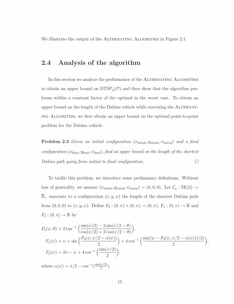
Problem 2.3 Given an initial configuration (xinitial, yinitial, ψinitial) and a final

configuration (xfinal, yfinal, ψfinal), find an upper bound on the length of the shortest

Dubins path going from initial to final configuration.

To tackle this problem, we introduce some preliminary definitions. Without

loss of generality, we assume (xinitial, yinitial, ψinitial) = (0, 0, 0). Let Cρ : SE(2) →

R+ associate to a configuration (x, y, ψ) the length of the shortest Dubins path

from (0, 0, 0) to (x, y, ψ). Define F0 : (0, π)× (0, π) → (0, π), F1 : (0, π) → R and

F2 : (0, π] → R by

F0(ψ, θ) = 2 tan−1( sin(ψ/2) − 2 sin(ψ/2 − θ)

cos(ψ/2) + 2 cos(ψ/2 − θ)

),

F1(ψ) = ψ + sin(F0(ψ, ψ/2 − α(ψ))

2

)+ 4 cos−1

(sin((ψ − F0(ψ, ψ/2 − α(ψ)))/2)

2

),

F2(ψ) = 2π − ψ + 4 cos−1(sin(ψ/2)

2

),

where α(ψ) = π/2 − cos−1( sin(ψ/2)2

).

15

Figure 2.1: An application of the Alternating Algorithm. Left figure: a

graph representing the solution of ETSP over a given P . Right figure: a graph

representing the solution given by the Alternating Algorithm on P where

the alternate segments of ETSP are retained.

Theorem 2.4 (Upper bound on optimal point-to-point length) For ψ ∈

[0, 2π[, (x, y) ∈ R2, and ρ > 0,

Cρ(x, y, ψ) ≤√x2 + y2 + κπρ,

where κ ∈ [2.657, 2.658] is defined by κ = 1π

maxF2(π), supψ∈]0,π[ minF1(ψ), F2(ψ).

It is a conjecture that κ = 7/3; we provide some numerical evidence in Ap-

pendix A.3. Next, we let LAA,ρ(P ) denote the length of Dubins path as given by

the Alternating Algorithm for a point set P . The following lemma estab-

lishes bounds on the performance of the Alternating Algorithm.

Lemma 2.5 (Upper bound on the performance of the Alternating Algo-

rithm) For any P ∈ Pn with n > 2 and ρ > 0,

LAA,ρ(P ) ≤ ETSP(P ) + κ⌈n

2

⌉πρ.

16

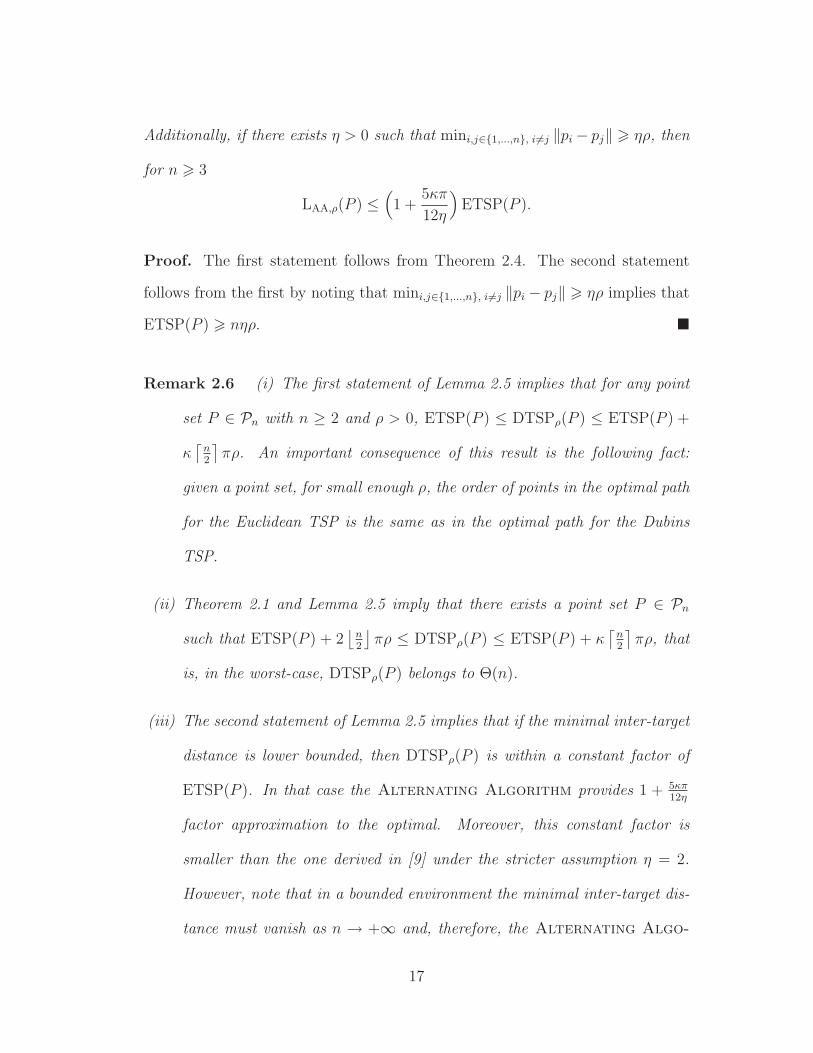
Additionally, if there exists η > 0 such that mini,j∈1,...,n, i6=j ‖pi− pj‖ > ηρ, then

for n > 3

LAA,ρ(P ) ≤(1 +

5κπ

12η

)ETSP(P ).

Proof. The first statement follows from Theorem 2.4. The second statement

follows from the first by noting that mini,j∈1,...,n, i6=j ‖pi − pj‖ > ηρ implies that

ETSP(P ) > nηρ.

Remark 2.6 (i) The first statement of Lemma 2.5 implies that for any point

set P ∈ Pn with n ≥ 2 and ρ > 0, ETSP(P ) ≤ DTSPρ(P ) ≤ ETSP(P ) +

κ⌈n2

⌉πρ. An important consequence of this result is the following fact:

given a point set, for small enough ρ, the order of points in the optimal path

for the Euclidean TSP is the same as in the optimal path for the Dubins

TSP.

(ii) Theorem 2.1 and Lemma 2.5 imply that there exists a point set P ∈ Pn

such that ETSP(P ) + 2⌊n2

⌋πρ ≤ DTSPρ(P ) ≤ ETSP(P ) + κ

⌈n2

⌉πρ, that

is, in the worst-case, DTSPρ(P ) belongs to Θ(n).

(iii) The second statement of Lemma 2.5 implies that if the minimal inter-target

distance is lower bounded, then DTSPρ(P ) is within a constant factor of

ETSP(P ). In that case the Alternating Algorithm provides 1 + 5κπ12η

factor approximation to the optimal. Moreover, this constant factor is

smaller than the one derived in [9] under the stricter assumption η = 2.

However, note that in a bounded environment the minimal inter-target dis-

tance must vanish as n → +∞ and, therefore, the Alternating Algo-

17

rithm is a constant factor approximation algorithm only for finite point

sets with lower bounded inter-target distance.

Having established bounds on the performance of the Alternating Algo-

rithm, we now show that it performs within a constant factor of the optimal for

the worst-case point sets.

Theorem 2.7 (Performance of the Alternating Algorithm for the worst-

case point sets) For n ≥ 2, P ∈ Pn and ρ > 0,

DTSPρ(P ) ≤ LAA,ρ(P ) ≤ ETSP(P ) + κ⌈n/2⌉πρ supP∈Pn

DTSPρ(P )

ETSP(P ) + 2⌊n/2⌋πρ.

Furthermore,

lim supn→+∞

LAA,ρ(P )

supP∈PnDTSPρ(P )

≤ κ

2.

Proof. The first statement follows from the simple fact that LAA,ρ(P ) ≥ DTSPρ(P ),

and from the results in Lemma 2.5 and Theorem 2.1. To prove the second state-

ment, we take the limit as n→ +∞ in the first statement and we use the bound

in equation (2.1).

Remark 2.8 For P ∈ Pn, Lemma 2.5 implies that LAA,ρ(P ) belongs to O(n)

and Theorem 2.7 implies that in the worst case, DTSPρ(P ) belongs to Θ(n) and

that the Alternating Algorithm performs within κ2

factor of the optimal for

the worst-case point sets. The computational complexity of the Alternating

Algorithm is of order n.

18

2.5 Summary

In this chapter, we have formulated and studied the TSP for vehicles that

follow paths of bounded curvature in the plane. For the worst-case setting, we

have obtained an upper bound that is within a constant factor of the lower

bound; the upper bound is constructive in the sense that it is achieved by a novel

algorithm. It is interesting to compare our results with the Euclidean setting

(i.e., the setting in which vehicle paths do not have curvature constraints). For

a given compact set and a point set P of n points, it is known [18, 19] that

the ETSP(P ) belongs to Θ(√n). This is true for both stochastic and worst-case

settings. In this chapter, we showed that, given a fixed ρ > 0, the DTSPρ(P ) in

the worst case belongs to Θ(n). In the next chapter, we study stochastic DTSP

and DTRP.

19

Chapter 3

DTSP: The stochastic and the

dynamic case

The discussion in the previous chapter showed that the Alternating Al-

gorithm performs well when the points to be visited by the tour are chosen in an

adversarial manner. However, this algorithm is not a constant-factor approxima-

tion algorithm in the general case. Moreover, this algorithm might not perform

very well when dealing with a random distribution of the target points. In this

chapter we study a stochastic version of the DTSP where the n targets are ran-

domly sampled from a uniform distribution. We show that the expected length

of such a tour is of order at least n2/3 and we propose a novel algorithm yielding

a solution with length of order n2/3 with high probability. Additionally, we study

a dynamic version of the DTSP: given a stochastic process that generates target

points, is there a policy which guarantees that the number of unvisited points

does not diverge over time? If such stable policies exist, what is the minimum

20

expected time that a newly generated target waits before being visited by the

vehicle? We propose a novel stabilizing algorithm such that the expected wait

time is provably within a constant factor from the optimum.

We make the following assumptions: Q is a rectangle of width W and height

H with W ≥ H; different choices for the shape of Q affect our conclusions only

by a constant. The two axes of the reference frame are parallel to the sides of Q.

3.1 Lower bound for the stochastic DTSP

For the stochastic DTSP, we assume that the points P = (p1, . . . , pn) are

randomly generated according to a uniform distribution in Q.

We begin with a result from [40] that provides a lower bound on the expected

length of the stochastic DTSP.

Theorem 3.1 (Lower bound on stochastic DTSP) Let P ∈ Pn be uniformly,

randomly and independently generated in the rectangle of width W and height H.

For any ρ > 0,

lim infn→+∞

E[DTSPρ(P )]

n2/3≥ 3

43√

3ρWH.

Remark 3.2 Theorem 3.1 implies that E[DTSPρ(P )] belongs to Ω(n2/3).

21

3.2 The basic geometric construction

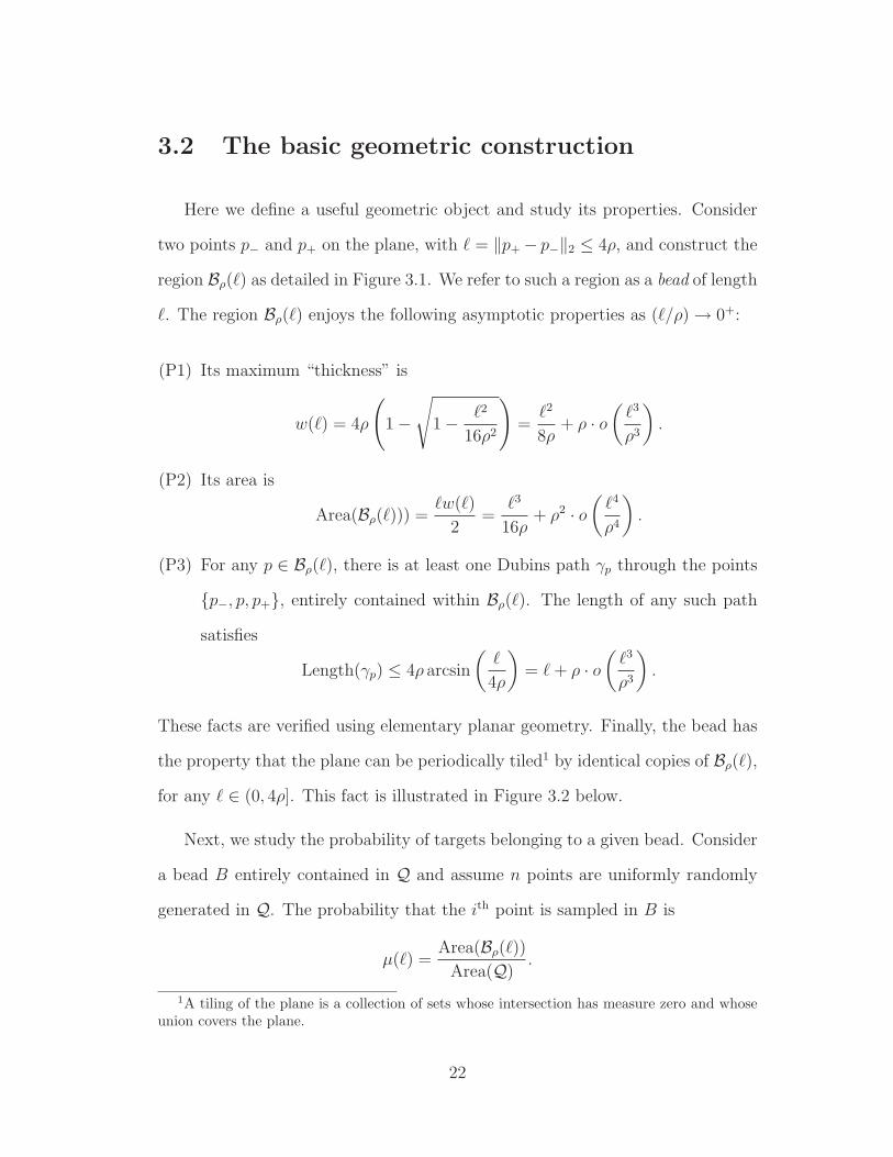
Here we define a useful geometric object and study its properties. Consider

two points p− and p+ on the plane, with ℓ = ‖p+ − p−‖2 ≤ 4ρ, and construct the

region Bρ(ℓ) as detailed in Figure 3.1. We refer to such a region as a bead of length

ℓ. The region Bρ(ℓ) enjoys the following asymptotic properties as (ℓ/ρ) → 0+:

(P1) Its maximum “thickness” is

w(ℓ) = 4ρ

(1 −

√

1 − ℓ2

16ρ2

)=ℓ2

8ρ+ ρ · o

(ℓ3

ρ3

).

(P2) Its area is

Area(Bρ(ℓ))) =ℓw(ℓ)

2=

ℓ3

16ρ+ ρ2 · o

(ℓ4

ρ4

).

(P3) For any p ∈ Bρ(ℓ), there is at least one Dubins path γp through the points

p−, p, p+, entirely contained within Bρ(ℓ). The length of any such path

satisfies

Length(γp) ≤ 4ρ arcsin

(ℓ

4ρ

)= ℓ+ ρ · o

(ℓ3

ρ3

).

These facts are verified using elementary planar geometry. Finally, the bead has

the property that the plane can be periodically tiled1 by identical copies of Bρ(ℓ),

for any ℓ ∈ (0, 4ρ]. This fact is illustrated in Figure 3.2 below.

Next, we study the probability of targets belonging to a given bead. Consider

a bead B entirely contained in Q and assume n points are uniformly randomly

generated in Q. The probability that the ith point is sampled in B is

µ(ℓ) =Area(Bρ(ℓ))

Area(Q).

1A tiling of the plane is a collection of sets whose intersection has measure zero and whoseunion covers the plane.

22

ρ

p−

p+

Bρ(ℓ)

ℓ

Figure 3.1: Construction of the “bead” Bρ(ℓ). The figure shows how the upper

half of the boundary is constructed, the bottom half is symmetric.

Furthermore, the probability that exactly k out of the n points are sampled in B

has a binomial distribution, i.e., indicating with nB the total number of points

sampled in B,

Pr[nB = k| n samples] =

(n

k

)µk(1 − µ)n−k.

If the bead length ℓ is chosen as a function of n in such a way that ν = n ·µ(ℓ(n))

is a constant, then the limit for large n of the binomial distribution is [41] the

Poisson distribution of mean ν, that is,

limn→+∞

Pr[nB = k| n samples] =νk

k!e−ν .

3.3 The Recursive Bead-Tiling Algorithm

In this section, we design a novel algorithm that computes a Dubins path

through a point set in Q. The proposed algorithm consists of a sequence of phases;

23

during each phase, a Dubins tour (i.e., a closed path with bounded curvature)

is constructed that “sweeps” the set Q. We begin by considering a tiling of

the plane such that Area(Bρ(ℓ)) = WH/(2n); in such a case, µ(ℓ(n)) = 1/(2n),

ν = 1/2, and

ℓ(n) = 2(ρWH

n

) 13

+ o(n− 1

3

), (n→ +∞).

(Note that this implies that n must be large enough in order that ℓ ≤ 4ρ.)

Furthermore, the tiling is chosen in such a way that it is aligned with the sides of

Q, see Figure 3.2. In the first phase of the algorithm, a Dubins tour is constructed

with the following properties:

(i) it visits all non-empty beads once,

(ii) it visits all rows2 in sequence top-to-bottom, alternating between left-to-

right and right-to-left passes, and visiting all non-empty beads in a row,

(iii) when visiting a non-empty bead, it services at least one target in it.

In order to visit the targets outstanding after the first phase, a second phase

is initiated. Instead of considering single beads, we now consider “meta-beads”

composed of two beads each, as shown in Figure 3.2, and proceed in a way similar

to the first phase, i.e., a Dubins tour is constructed with the following properties:

(i) the tour visits all non-empty meta-beads once,

(ii) it visits all (meta-bead) rows in sequence top-to-down, alternating between

left-to-right and right-to-left passes, and visiting all non-empty meta-beads

in a row,

2A row is a maximal sequence of horizontally-aligned beads with non-empty intersectionwith Q.

24

(iii) when visiting a non-empty meta-bead, it services at least one target in it.

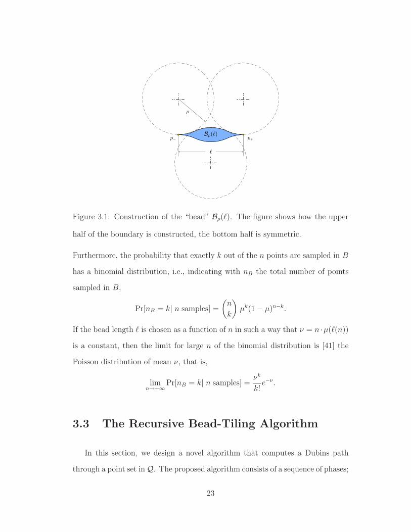
Figure 3.2: Sketch of “meta-beads” at successive phases in the recursive bead

tiling algorithm. From left to right: phase 1, phase 2 and phase 3. Note that

for phase 2 (and for all subsequent even-numbered phases), the vehicle will have

to visit every row of meta-beads twice, once to visit targets in the meta-beads

with the darker shade and once to visit targets in the meta-beads with the lighter

shade.

This process is iterated ⌈log2 n⌉ times, and at each phase, meta-beads com-

posed of two neighboring meta-beads from the previous phase are considered; in

other words, the meta-beads at the ith phase are composed of 2i−1 neighboring

beads. After the last recursive phase, the leftover targets are visited using the

Alternating Algorithm.

3.4 Analysis of the algorithm

In this section, we calculate an upper bound on the length of Dubins path

as given by the Recursive Bead-Tiling Algorithm. By comparing this

upper bound with the lower bound established earlier, we will conclude that the

algorithm provides a constant factor approximation to the optimal stochastic

DTSP with high probability. We begin with a key result about the number of

25

outstanding targets after the execution of the ⌈log2 n⌉ recursive phases; the proof

of this result is based upon techniques similar to those developed in [42].

Theorem 3.3 (Targets remaining after recursive phases) Let P ∈ Pn be

uniformly randomly generated in Q. The number of unvisited targets after the

last recursive phase of the Recursive Bead-Tiling Algorithm over P is

less than 24 log2 n with high probability, i.e., with probability approaching one as

1 − log2 2nn2 .

Proof. Associate a unique identifier to each bead, let b(t) be the identifier of the

bead in which the tth target is sampled, and let h(t) ∈ N be the phase at which

the tth target is visited. Without loss of generality, assume that targets within

a single bead are visited in the same order in which they are generated, i.e., if

b(t1) = b(t2) and t1 < t2, then h(t1) < h(t2). Note that we assume here that only

one target per bead is visited at each phase. The resultant analysis will give an

upper bound on the path length for the Recursive Bead-Tiling Algorithm.

Let vi(t) be the number of beads that contain unvisited targets at the inception

of the ith phase, computed after the insertion of the tth target. Furthermore,

let mi be the number of ith phase meta-beads (i.e., meta-beads containing 2i−1

neighboring beads) with a non-empty intersection with Q. Clearly, vi(t) ≤ vi(n),

mi ≤ 2mi+1, and v1(n) ≤ n ≤ m1/2 with certainty. The tth target will not be

visited during the first phase if it is sampled in a bead that already contains other

targets. In other words,

Pr[h(t) ≥ 2| v1(t− 1)

]=v1(t− 1)

m1

≤ v1(n)

2n≤ 1

2.

Similarly, the tth target will not be visited during the ith phase if (i) it has not

been visited before the ith pass, and (ii) it belongs to a meta-bead that already

26

contains other targets not visited before the ith phase:

Pr[h(t) ≥ i+ 1| (vi(t− 1), vi−1(t− 1), . . . , v1(t− 1))

]

= Pr[h(t) ≥ i+ 1| h(t) ≥ i, vi(t− 1)

]

· Pr[h(t) ≥ i| (vi−1(t− 1), . . . , v1(t− 1))

]

≤ vi(t− 1)

mi

Pr[h(t) ≥ i| (vi−1(t− 1), . . . , v1(t− 1))]

=i∏

j=1

vj(t− 1)

mj

≤i∏

j=1

2j−1vj(n)

2n=

(2

i−32

n

)i i∏

j=1

vj(n).

Given a sequence βii∈N ⊂ R+ and given a fixed i ≥ 1, define a sequence of

binary random variables

Yt(i) =

1, if h(t) ≥ i+ 1 and vi(t− 1) ≤ βin,

0, otherwise.

In other words, Yt(i) = 1 if the tth target is not visited during the first i phases

even though the number of beads still containing unvisited targets at the inception

of the ith phase is less than βin. Even though the random variable Yt(i) depends

on the targets generated before the tth target, the probability that it takes the

value 1 is bounded by

Pr[Yt(i) = 1| b(1), b(2), . . . , b(t− 1)] ≤ 2i(i−3)

2

i∏

j=1

βj =: qi,

regardless of the actual values of b(1), . . . , b(t − 1). It is known [42] that if the

random variables Yt(i) satisfy such a condition, the sum∑

t Yt(i) is stochastically

dominated by a binomially distributed random variable, namely,

Pr

[n∑

t=1

Yt(i) > k

]≤ Pr[B(n, qi) > k],

27

where B(n, qi) denotes a binomially distributed random variable with parameters

n and qi. In particular,

Pr

[n∑

t=1

Yt(i) > 2nqi

]≤ Pr[B(n, qi) > 2nqi] < 2−nqi/3, (3.1)

where the last inequality follows from Chernoff’s Bound [41]. Now, it is convenient

to define βii∈N by

β1 = 1, βi+1 = 2qi = 2i(i−3)

2+1

i∏

j=1

βj = 2i−2 β2i ,

which leads to βi = 21−i. In turn, this implies that equation (3.1) can be rewritten

as

Pr

[n∑

t=1

Yt(i) > βi+1n

]< 2−βi+1n/6 = 2−

n

3·2i ,

which is less than 1/n2 for i ≤ i∗(n) := ⌊log2 n − log2 log2 n − log2 6⌋ ≤ log2 n.

Note that βi ≤ 12 log2 nn

, for all i > i∗(n).

Let Ei be the event that vi(n) ≤ βin. Note that if Ei is true, then vi+1(n) ≤∑n

t=1 Yt(i): the right hand side represents the number of targets that will be

visited after the ith phase, whereas the left hand side counts the number of beads

containing such targets. We have, for all i ≤ i∗(n):

Pr[vi+1(n) > βi+1n| Ei

]· Pr[Ei] ≤ Pr

[n∑

t=1

Yt(i) > βi+1n

]≤ 1

n2,

that is, Pr [¬Ei+1| Ei] ·Pr[Ei] ≤1

n2, and thus (recall that E1 is true with certainty):

Pr [¬Ei+1] = Pr [¬Ei+1| Ei] ·Pr[Ei] +Pr [¬Ei+1| ¬Ei] ·Pr[¬Ei] ≤1

n2+Pr[¬Ei] ≤

i

n2.

In other words, for all i ≤ i∗(n), vi(n) ≤ βin with high probability.

Let us now turn our attention to the phases such that i > i∗(n). The total

number of targets visited after the (i∗)th phase is dominated by a binomial variable

28

B(n, 12 log2 n/n); in particular,

Pr[vi∗+1(n) > 24 log2 n| Ei∗

]· Pr[Ei∗ ] ≤ Pr

[ n∑

t=1

Yt(i) > 24 log2 n]

≤ Pr[B(n, 12 log2 n/n) > 24 log2 n

]

≤ 2−12 log2 n.

Dealing with conditioning as before, we obtain

Pr [vi∗+1(n) > 24 log2 n] ≤ 1

n12+ Pr[¬Ei∗ ] ≤

1

n12+

log2 n

n2. (3.2)

In other words, the number of unvisited targets after the (i∗)th phase is bounded

by a logarithmic function of n with high probability. Equation (3.2) also shows

that this probability approaches one as 1 − log2 2nn2 .

In summary, Theorem 3.3 says that after a sufficiently large number of phases,

almost all targets will be visited, with high probability. A simple application of

the Borel-Cantelli Lemma [43] to the upper bound in equation (3.2) gives the

following corollary.

Corollary 3.4 With probability one, the number of unvisited targets after the

last recursive phase of the Recursive Bead-Tiling Algorithm over P is

less than 24 log2 n asymptotically.

We also observe that (i) the length of the first phase is of order n2/3 and (ii)

the length of each phase is decreasing at such a rate that the sum of the lengths

of the ⌈log2 n⌉ recursive phases remains bounded and proportional to the length

of the first phase. (Since we are considering the asymptotic case in which the

number of targets is very large, the length of the beads will be very small; in

29

the remainder of this section we will tacitly consider the asymptotic behavior as

ℓ/ρ→ 0+.)

Lemma 3.5 (Path length for the first phase) Consider a tiling of the plane

with beads of length ℓ. For any ρ > 0 and for any set of target points, the length

L1 of a path visiting once and only once each bead with a non-empty intersection

with a rectangle Q of width W and length H satisfies

L1 ≤16ρWH

ℓ2

(1 +

7

3πρ

W

)+ ρ · o

(ρℓ

).

Proof. A path visiting each bead once can be constructed by a sequence of

passes, during which all beads in a row are visited in a left-to-right or right-to-

left order. In each row, there are at most ⌈W/ℓ⌉ + 1 beads with a non-empty

intersection with Q. Hence, the cost of each pass is at most:

Lpass1 ≤ W + 2ℓ+ ρ · o

(ℓ2

ρ2

).

Two passes are connected by a U-turn maneuver, in which the direction of

travel is reversed, and the path moves to the next row, at distance equal to one

half the width of a bead. Since the length of the shortest path to reverse the

heading of a Dubins vehicle with co-located initial and final points is (7/3)πρ,

the length of the U-turn satisfies

LU−turn1 ≤ 7

3πρ+

1

2w(ℓ) ≤ 7

3πρ+

ℓ2

16ρ+ ρ · o

(ℓ3

ρ3

).

The total number of passes, i.e., the total number of rows of beads with non-

empty intersection with Q, satisfies

Npass1 ≤

⌈2H

w(ℓ)

⌉+ 1 ≤ 16ρH

ℓ2+ 2 + o

(ρℓ

).

30

A simple upper bound on the cost of closing the tour is given by

Lclose1 ≤ (W + 2ℓ) + (H + 2w(ℓ)) + 2πρ = W +H + 2πρ+ 2ℓ+ ρ · o(ℓ/ρ).

In summary, the total length of the path followed during the first phase is

L1 ≤Npass1

(Lpass

1 + LU−turn1

)+ Lclose

≤(

16ρH

ℓ2+ 2 + o

(ρℓ

))(W + 2ℓ+

7

3πρ+

ℓ2

16ρ+ ρ · o

(ℓ2

ρ2

))

+W +H + 2πρ+ 2ℓ+ ρ · o(ℓ/ρ)

≤16ρWH

ℓ2

(1 +

7

3πρ

W

)+ ρ · o

(ρℓ

).

Based on this calculation, we can estimate the length of the paths in generic

phases of the algorithm. Since the total number of phases in the algorithm

depends on the number of targets n, as does the length of the beads ℓ, we will

retain explicitly the dependency on the phase number.

Lemma 3.6 (Path length at odd-numbered phases) Consider a tiling of the

plane with beads of length ℓ. For any ρ > 0 and for any set of target points, the

length L2j−1 of a path visiting once and only once each meta-bead with a non-

empty intersection with a rectangle Q of width W and length H at phase number

(2j − 1), j ∈ N satisfies

L2j−1 ≤ 25−j[ρWH

ℓ2

(1 +

7

3

πρ

W

)+ ρ · o

(ρℓ

)]+32

ρH

ℓ+ρ·o

(ρℓ

)+2j

[3ℓ+ ρ · o

(ℓ

ρ

)].

Proof. During odd-numbered phases, the number of beads in a meta-bead is a

perfect square and the considerations made in the proof of Lemma 3.5 can be

31

readily adapted. The length of each pass satisfies

Lpass2j−1 ≤

(W + 2jℓ

) [1 + o

(ℓ

ρ

)].

The length of each U-turn maneuver is bounded as

LU−turn2j−1 ≤ 7

3πρ+ 2j−2w(ℓ) ≤ 7

3πρ+ 2j−2

[ℓ2

8ρ+ ρ · o

(ℓ3

ρ3

)],

from which

Lpass2j−1 + LU−turn

2j−1 = W +7

3πρ+ o

(ℓ

ρ

)+ 2j

[ℓ+ ρ · o

(ℓ

ρ

)].

The number of passes satisfies:

Npass2j−1 ≤ 25−j

[ρH

ℓ2+ o

(ρℓ

)]+ 2.

Finally, the cost of closing the tour is bounded by

Lclose2j−1 ≤ W +H + 2πρ+ 2j [ℓ+ ρ · o(ℓ/ρ)] .

Therefore, a bound on the total length of the path is

L2j−1 = Npass2j−1(L

pass2j−1 + LU−turn

2j−1 ) + Lclose2j−1

≤ 25−j[ρWH

ℓ2

(1 +

7

3

πρ

W

)+ ρ · o

(ρℓ

)]+32

ρH

ℓ+ρ·o

(ρℓ

)+2j

[3ℓ+ ρ · o

(ℓ

ρ

)].

Lemma 3.7 (Path length at even-numbered phases) Consider a tiling of

the plane with beads of length ℓ. For any ρ > 0, a rectangle Q of width W and

length H and any set of target points, paths in each phase of the algorithm can

be chosen such that L2j ≤ 2L2j+1, for all j ∈ N.

32

Proof. Consider a generic meta-bead B2j+1 traversed in the (2j+1)th phase, and

let l3 be the length of the path segment within B2j+1. The same meta-bead is

traversed at most twice during the (2j)th phase; let l1, l2 be the lengths of the two

path segments of the (2j)th phase within B2j+1. By convention, for i ∈ 1, 2, 3,

we let li = 0 if the ith path does not intersect B2j+1. Without loss of generality,

the order of target points can be chosen in such a way that l1 ≤ l2 ≤ l3, and

hence l1 + l2 ≤ 2l3. Repeating the same argument for all non-empty meta-beads,

we prove the claim.

Finally, we can summarize these intermediate bounds into the main result of

this section. We let LRBTA,ρ(P ) denote the length of the Dubins path computed

by the Recursive Bead-Tiling Algorithm for a point set P .

Theorem 3.8 (Path length for the Recursive Bead-Tiling Algorithm)

Let P ∈ Pn be uniformly, randomly and independently generated in the rectangle

of width W and height H. For any ρ > 0, with probability one,

lim supn→+∞

DTSPρ(P )

n2/3≤ lim sup

n→+∞

LRBTA,ρ(P )

n2/3≤ 24 3

√ρWH

(1 +

7

3πρ

W

).

Proof. For simplicity we let LRBTA,ρ(P ) = LRBTA. Clearly, LRBTA = L′RBTA +

L′′RBTA, where L′

RBTA is the path length of the first ⌈log2 n⌉ phases of the algorithm

and L′′BTA is the length of the path required to visit all remaining targets. An

immediate consequence of Lemma 3.7, is that

L′RBTA =

⌈log2(n)⌉∑

i=1

Li ≤ 3

⌈log2(n)/2⌉∑

j=1

L2j−1.

33

The summation on the right hand side of this equation can be expanded using

Lemma 3.6, yielding

L′RBTA ≤ 3

[ρWH

ℓ2

(1 +

7

3

πρ

W

)+ ρ · o

(ρ2

ℓ2

)] ⌈log2(n)/2⌉∑

j=1

25−j

+

(32ρH

ℓ+ ρ · o

(ρℓ

))⌈ log2 n

2

⌉+ [3ℓ+ ρ · o(ℓ/ρ)]

⌈log2(n)/2⌉∑

j=1

2j

.

Since∑k

j=1 2−j ≤ ∑+∞j=1 2−j = 1, and

∑kj=1 2j = 2k+1 − 2 ≤ 2k+1, the previous

equation can be simplified to

L′RBTA ≤ 3

32

[ρWH

ℓ2

(1 +

7

3

πρ

W

)+ ρ · o

(ρℓ

)]

+

(32ρH

ℓ+ ρ · o

(ℓ

ρ

))⌈log2 n

2

⌉+ [3ℓ+ ρ · o(ℓ/ρ)] · (4√n)

.

Recalling that ℓ = 2(ρWH/n)1/3+o(n−1/3) for large n, the above can be rewritten

as

L′RBTA ≤ 24 3

√ρWHn2

(1 +

7

3πρ

W

)+ o(n2/3).

Now it suffices to show that L′′RBTA is negligible with respect to L′

RBTA for large

n with high probability. From Theorem 3.3, we know that with high probabil-

ity there will be at most 24 log2 n unvisited targets after the ⌈log2 n⌉ recursive

phases. From Lemma 2.5 we know that, with high probability, the length of a

Alternating Algorithm tour through these points satisfies

L′′RBTA ≤ κ⌈12 log2 n⌉πρ+ o(log2 n).

Next, we state a result for the concentration of DTSPρ(P ) around its mean,

which will let us compare the lower bound in Theorem 3.1 with the upper bound

in Theorem 3.8.

34

Lemma 3.9 (Concentration around the mean) Let P ∈ Pn be uniformly,

randomly and independently generated in the rectangle of width W and height H.

For any ρ > 0, with probability one,

|DTSPρ(P ) − E[DTSPρ(P )]| ∈ O(√n log n).

Proof. The proof presented here closely follows the one for the Long Common

Sub-sequence Problem in Chapter 1 of [44]. We use Doob’s method to construct

a martingale from the random variable DTSPρ(P ). First let Fk = σ(p1, . . . , pk),

that is, Fk is the sigma-field generated by the first k elements of P = p1, . . . , pn,

and then we set

di = E[DTSPρ(P )|Fi] − E[DTSPρ(P )|Fi−1].

The sequence di can be easily checked to be a martingale-difference sequence

adapted to the increasing sequence of sigma-fields Fi. Moreover, di’s are related

to the original variables via the following relation:

DTSPρ(P ) − E[DTSPρ(P )] =n∑

i=1

di.

Consider a new sequence of independent random variables pi with the same dis-

tribution as the original pi. Accordingly, define Pi := p1, . . . , pi−1, pi, pi+1, . . . , pn.

Since Fi has no information about pi, we have

E[DTSPρ(P )|Fi−1] = E[DTSPρ(Pi)|Fi],

and this representation then lets us rewrite the expression for di in terms of a

single conditional expectation:

di = E[DTSPρ(P ) − DTSPρ(Pi)|Fi].

35

From Theorem 2.4, one can easily check that

|DTSPρ(P ) − DTSPρ(Pi)| ≤ 2 diamQ + 2κπρ =: c.

Since conditional expectations cannot increase the upper bound, we have |di| ≤ c

for all i ∈ 1, . . . , n. Finally, by Azuma’s Inequality, we have the useful tail

bound:

Pr[|DTSPρ(P ) − E[DTSPρ(P )]| ≥ t

]≤ 2 exp

(− t2/(2nc2)

).

Applying the Borel-Cantelli Lemma with t =√

2c2n(log n)(1 + ǫ), where ǫ is

some positive constant, gives us the desired result.

Remark 3.10 Lemma 3.9 implies that, with probability one,

limn→+∞

(DTSPρ(P )

n2/3− E[DTSPρ(P )]

n2/3

)= 0.

This statement together with Theorems 3.1 and 3.8 implies that, with probability

one, the Recursive Bead-Tiling Algorithm is a (32/3√

3)(1 +

7

3πρ

W

)fac-

tor approximation (with respect to n) to the optimal DTSP and that DTSPρ(P )

belongs to Θ(n2/3). The computational complexity of the Recursive Bead-

Tiling Algorithm is of order n.

3.4.1 Numerical Results

In this section we present numerical results for the Recursive Bead-Tiling

Algorithm.The results are summarized in the form of a logarithmic plot in Fig-

ure 3.3. The points comprising the set P are randomly and independently gen-

erated according to a uniform distribution in a rectangle of width W = 10 and

36

2 4 6 8 10 12

2

4

6

8

10

12

14log(LRBTA,ρ(P ))

log(n)

Figure 3.3: Plot of log(LRBTA,ρ(P )) vs. log(n)

height H = 8. The minimum turning radius for the Dubins vehicle is ρ = 1.

Each point represents the mean of Dubins path length as given by the Re-

cursive Bead-Tiling Algorithm, taken over 10 instances of the experiment

for the corresponding values of n. The lower solid line represents the function

log(Cln

2/3)

where Cl is the value of the quantity 34

3√

3ρWH corresponding to the

lower bound in Theorem 3.1. Similarly, the upper solid line represents the func-

tion log(Cun

2/3), with Cu being the value of 24 3

√ρWH

(1 + 7

3π ρW

)corresponding

to the upper bound in Theorem 3.8. From the simulations we gather the following

qualitative observations. First, the lower bound to DTSPρ(P ) established in The-

orem 3.1 is fairly conservative when considered as a lower bound to LRBTA,ρ(P ).

Second, the upper bound to LRBTA,ρ(P ) established in Theorem 3.8 becomes less

conservative and the data conforms more accurately with the 2/3 exponent as n

grows.

37

3.5 The DTRP for a single vehicle

We now turn our attention to the Dynamic Traveling Repairperson Problem

(DTRP) that was introduced by Bertsimas and van Ryzin in [24]. When com-

pared with previous work, the novel feature of the following work is the focus on

the Dubins vehicle.

3.5.1 Model and problem statement

In this subsection we describe the vehicle and sensing model and the DTRP

definition. The key aspect of the DTRP is that the Dubins vehicle is required to

visit a dynamically growing set of targets, generated by some stochastic process.

We assume that the Dubins vehicle has unlimited range and target-servicing

capacity and that it moves at a unit speed with minimum turning radius ρ > 0.

Information about the outstanding targets representing the demand at time

t is described by a finite set of positions D(t) ⊂ Q, with n(t) := card(D(t)).

Targets are generated, and inserted into D, according to a homogeneous (i.e.,

time-invariant) spatio-temporal Poisson process, with time intensity λ > 0, and

uniform spatial density inside the rectangle Q of width W and height H. In other

words, given a set S ⊆ Q, the expected number of targets generated in S within

the time interval [t, t′] is

E[card(D(t′) ∩ S) − card(D(t) ∩ S)

]= λ(t′ − t) Area(S).

(Strictly speaking, the above equation holds when targets are not being removed

from the queue D.) Servicing of a target and its removal from the set D, is

achieved when the Dubins vehicle moves to the target position.

38

A feedback control policy for the Dubins vehicle is a map Φ assigning a control

input to the vehicle as a function of its configuration and of the current outstand-

ing targets. We also consider policies that compute a control input based on a

snapshot of the outstanding target configurations at certain time sequences. Let

TΦ = tkk∈N be a strictly increasing sequence of times at which such computa-

tions are started: with some abuse of terminology, we will say that Φ is a receding

horizon strategy if it is based on the most recent target data Drh(t), where

Drh(t) = D(maxtrh ∈ TΦ | trh ≤ t).

The (receding horizon) policy Φ is a stable policy for the DTRP if, under its

action

nΦ = limt→+∞

E[n(t)| p = Φ(p,Drh)] < +∞,

that is, if the Dubins vehicle is able to service targets at a rate that is, on average,

at least as fast as the rate at which new targets are generated. Let Tj be the time

that the jth target spends within the set D, i.e., the time elapsed from the time

the jth target is generated to the time it is serviced. If the system is stable, then

we can write the balance equation (known as Little’s formula [45]):

nΦ = λTΦ,

where TΦ := limj→+∞ E[Tj] is the steady-state system time for the DTRP under

the policy Φ. Our objective is to minimize the steady-state system time, over all

possible feedback control policies, i.e.,

TDTRP = infTΦ | Φ is a stable control policy.

39

3.5.2 Lower and constructive upper bounds

In what follows, we design a control policy that provides a constant-factor

approximation of the optimal achievable performance. Consistently with the

theme of the chapter, we consider the case of heavy load, i.e., the problem as

the time intensity λ → +∞. We first review from [40] a lower bound for the

system time, and then present a novel approximation algorithm providing an

upper bound on the performance.

Theorem 3.11 (Lower bound on the system time for the DTRP) For any ρ > 0,

the system time TDTRP for the DTRP in a rectangle of width W and height H

satisfies

lim infλ→+∞

TDTRP

λ2≥ 81

64ρWH.

Remark 3.12 Theorem 3.11 implies that the system time for the Dubins vehicle

depends quadratically on the time intensity λ, whereas in the Euclidean case it

depends only linearly on it, e.g., see [24].

We now propose a simple strategy, the Bead-Tiling Algorithm, based

on the concepts introduced in the previous section. The strategy consists of the

following steps:

(i) Tile the plane with beads of length ℓ := minCBTA/λ, 4ρ, where

CBTA =7 −

√17

4

(1 +

7

3πρ

W

)−1

. (3.3)

(ii) Update D to contain information of all (and only) the outstanding targets.

40

(iii) Visit all non-empty beads once, visiting one target per non-empty bead.

(iv) Repeat step (ii).

The following result characterizes the system time for the closed loop system

induced by this algorithm and is based on the bound derived in Lemma 3.5.

Theorem 3.13 (System time for the Bead-Tiling Algorithm) For any ρ >

0 and λ > 0, the Bead-Tiling Algorithm is a stable policy for the DTRP

and the resulting system time TBTA satisfies:

lim supλ→+∞

TDTRP

λ2≤ lim sup

λ→+∞

TBTA

λ2≤ 70.5464 ρWH

(1 +

7

3πρ

W

)3

.

Proof. Consider a generic bead B, with non-empty intersection with Q. Target

points within B will be generated according to a Poisson process with rate λB

satisfying

λB = λArea(B ∩Q)

WH≤ λ

Area(B)

WH=

C3BTA

16ρWHλ2+ o

(1

λ2

).

The vehicle will visit B at least once every L1 time units, where L1 is the bound

on the length of a path through all beads, as computed in Lemma 3.5. As a

consequence, targets in B will be visited at a rate no smaller than

µB =C2

BTA

16ρWHλ2

(1 +

7

3πρ

W

)−1

+ o

(1

λ2

).

In summary, the expected time TB between the appearance of a target in B and

its servicing by the vehicle is no more than the system time in a queue with

Poisson arrivals at rate λB, and deterministic service rate µB. Such a queue is

called a M/D/1 queue in the literature [45], and its system time is known to be

TM/D/1 =1

µB

(1 +

1

2

λBµB − λB

).

41

Using the computed bounds on λB and µB, and taking the limit as λ→ +∞, we

obtain

limλ→+∞

TB

λ2≤ lim

λ→+∞

TM/D/1

λ2≤ 16ρWH

C2BTA

(1 + 7

3π ρW

)−1

(1 +

1

2

CBTA(1 + 7

3π ρW

)−1 − CBTA

).

(3.4)

Since equation (3.4) holds for any bead intersecting Q, the bound derived for

TB holds for all targets and is therefore a bound on TBTA. The expression on

the right hand side of (3.4) is a constant that depends on problem parameters

ρ, W , and H, and on the design parameter CBTA, as defined in equation (3.3).

Stability of the queue is established by noting that CBTA < (1 + 7/3 π ρ/W )−1.

Additionally, the choice of CBTA in equation (3.3) minimizes the right hand side

of (3.4) yielding the numerical bound in the statement.

Remark 3.14 The achievable performance of the Bead-Tiling Algorithm

provides a constant-factor approximation to the lower bound established in The-

orem 3.11. Also, there exists no stable policy for the DTRP when the targets

are generated in an adversarial worst-case fashion with λ ≥ (πρ)−1. This fact

is a consequence of the linear lower bound on the worst-case DTSP derived in

Theorem 2.1.

3.6 The DTRP for multiple vehicles

The DTRP problem that was introduced in the earlier section for a single

vehicle can be easily extended to the multiple vehicle case. In this section, we

first obtain a lower bound for the system time form homogeneous Dubins vehicles,

and then present a novel strategy providing an upper bound on the performance.

42

Theorem 3.15 (Lower bound on the system time for single-vehicle DTRP) For

any ρ > 0, the system time TDTRP,m for the DTRP for m vehicles in a rectangle

of width W and height H satisfies

lim infλ→+∞

TDTRP,m

λ2≥ 81

64

ρWH

m3.

Proof. Let us assume that a stabilizing policy is available. In such a case,

the number of outstanding targets approaches a finite steady-state value, n∗,

related to the system time by Little’s formula, i.e., n∗ = λTDTRP,m. In order for

the policy to be stabilizing, the time needed, on average, to service m targets

must be no greater than the average time interval in which m new targets are

generated. Since there are m vehicles, the average time needed for them to service

one target each, in parallel, is no greater than the expected minimum distance

(in the Dubins’ sense) from an arbitrarily placed vehicle to the closest target; in

other words, we can write the stability condition E[δ∗(n∗)] ≤ m/λ. A bound on

the expected value of δ∗ has been computed in [40], yielding

3

4

(3ρWH

n∗

)1/3

≤ E[δ∗(n∗)] ≤ mλ.

Using Little’s formula n∗ = λTDTRP,m, and rearranging, we get the desired result.

From Theorem 3.13, one can infer that the system time depends on (i) the

area of the region assigned to a vehicle, and (ii) on the shape of the region.

In particular, the system time is minimized, for a given area, when one of its

dimensions is maximized. This suggest the following strategy for partitioning the

environment Q, that we call the Strip-Tiling Algorithm. Partition Q into

m strips of width W and height H/m and assign each strip to a vehicle. Tile

43

each strip with beads of length ℓ := minmCBTA/λ, 4ρ, where CBTA is given by

eq. (3.3). Let each vehicle execute the Bead-Tiling Algorithm inside the

assigned strip. Then, the following holds:

Theorem 3.16 (System time for the Strip-Tiling Algorithm) For any ρ >

0, λ > 0 and m > 0, the Strip-Tiling Algorithm is a stable policy for the

DTRP and the resulting system time TSTA,m satisfies:

lim supλ→+∞

TDTRP,m

λ2≤ lim sup

λ→+∞

TSTA,m

λ2≤ 70.5464

ρWH

m3

(1 +

7

3πρ

W

)3

.

Remark 3.17 The achievable performance of the Strip-Tiling Algorithm

provides a constant-factor approximation to the lower bound established in The-

orem 3.15.

3.7 Summary

In this chapter, we have studied the DTSP in the stochastic setting, and

obtained upper bounds that are within a constant factor of the lower bound;

the upper bounds are constructive in the sense that they are achieved by novel

algorithms. We showed that, given a fixed ρ > 0, the stochastic DTSPρ(P )

belongs to Θ(n2/3) with high probability.

Remarkably, the differences between these various bounds play a crucial role

when studying the DTRP; e.g., stable policies exist only when the TSP cost grows

strictly sub-linearly with n. For the DTRP we have proposed the novel policy

and shown its stability for a uniform target-generation process with intensity

λ. It is known [40] that the system time for the DTRP for the Dubins vehicle

44

belongs to Ω(λ2); the policy proposed in this chapter shows that the system time

belongs to O(λ2). Thus, the system time of the DTRP for the Dubins vehicle

belongs to Θ(λ2). This result differs from the result in the Euclidean case, where

it is known [24] that the system time belongs to Θ(λ). Therefore, our analysis

rigorously establishes the following intuitive fact: bounded-curvature constraints

make the system much more sensitive to increases in the target generation rate.

In the next chapter, we extend the analysis of this chapter to other vehicle

models and to the three-dimensional space.

45

Chapter 4

TSPs for a double integrator

In this chapter, we study path planning strategies for a double integrator

with bounded velocity and bounded control inputs. First, we study the following

version of the Traveling Salesperson Problem (TSP): given a set of points in Rd,

find the fastest tour over the point set for a double integrator. We first give

asymptotic bounds on the time taken to complete such a tour in the worst-

case. Then, we study a stochastic version of the TSP for double integrator

where the points are randomly sampled from a uniform distribution in a compact

environment in R2 and R

3. Lastly, we study the DTRP for a double integrator

in R2 as well as R

3.

This work completes the generalization of the known combinatorial results

on the ETSP and DTRP (applicable to systems with single integrator dynamics)

to double integrators and Dubins vehicle models. It is interesting to compare

our results with the setting where the vehicle is modeled by a single integrator

or the so-called Euclidean case in combinatorial optimization. The results are

46

summarized as follows:

Single Double Dubinsintegrator integrator vehicle

Min. time for Θ(n1− 1d ) [19] Ω(n1− 1

d ), Θ(n) [25]

TSP tour O(n1− 12d ) (d = 2, 3)

(worst-case)

Exp. min. time Θ(n1− 1d ) [19] Θ(n1− 1

2d−1 ) Θ(n1− 12d−1 )

for TSP tour w.h.p. w.h.p.(stochastic) (d = 2, 3) (d = 2, 3)

System time Θ(λd−1) [24] Θ(λ2(d−1)) Θ(λ2(d−1))for DTRP (d = 1) (d = 2, 3) (d = 2, 3)

4.1 Setup and worst-case DITSP

For d ∈ N, consider a vehicle with double integrator dynamics:

p(t) = u(t), ‖u(t)‖ ≤ rctr, ‖p(t)‖ ≤ rvel, (4.1)

where p ∈ Rd and u ∈ R

d are the position and control input of the vehicle,

rvel ∈ R+ and rctr ∈ R+ are the bounds on the attainable speed and control

inputs. Let Q ⊂ Rd be a unit hypercube. Let P = q1, . . . , qn be a set of n

points in Q and Pn be the collection of all point sets P ⊂ Q with cardinality n.

Let ETSP(P ) denote the cost of the Euclidean TSP over P and let DITSP(P )

denote the cost of the TSP for double integrator over P , i.e., the time taken

to traverse the fastest closed path for a double integrator through all points in

P . We assume rvel and rctr to be constant and we study the dependence of

DITSP: Pn → R+ on n. Without loss of generality, we assume the vehicle starts

traversing the TSP tour at t = 0 with initial position q1.

47

Lemma 4.1 (Worst-case Lower Bound on the TSP for Double Integrator) For

rvel, rctr ∈ R+ and d ∈ N, there exists a point set P ∈ Pn in Q ⊂ Rd such that

DITSP(P ) belongs to Ω(n1− 1d ).

Proof. We consider the class of point sets that give rise to the worst case

scenario for the ETSP; we refer the reader to [19]. It suffices to note that, for

such a point set of cardinality n in Rd, the minimum distance between any two

points belongs to Ω(n− 1d ). The minimum time required for a double integrator

with initial speed v to go from one point to another at a distance δ is lower

bounded by√

(v/rctr)2 + 2(δ/rctr) − v/rctr. However, v ≤ rvel and for the point

set under consideration, δ belongs to Ω(n− 1d ). This implies that the minimum

time required for a double integrator to travel between two points of the given

point set belongs to Ω(n− 1d ). Hence, the minimum time required for the vehicle

to complete the tour over this point set belongs to nΩ(n− 1d ), i.e., Ω(n1− 1

d ).

We now propose a simple strategy for the DITSP and analyze its performance.

The STOP-GO-STOP strategy can be described as follows: The vehicle visits the

points in the same order as in the optimal ETSP tour over the same set of points.

Between any pair of points, the vehicle starts at the initial point at rest, follows

the shortest-time path to reach the final point with zero velocity.

Theorem 4.2 (Upper Bound on the TSP for Double Integrator) For any point

set P ∈ Pn in Q ⊂ Rd and rctr > 0, rvel > 0 and d ∈ N, DITSP(P ) belongs to

O(n1− 12d ).

Proof. Without any loss of generality, let (q1, . . . , qn, q1) be the optimal order

of points for the Euclidean TSP over P . For 1 ≤ i ≤ n − 1, let δi = ‖qi − qi+1‖

48

and δn = ‖qn − q1‖. If δi is the distance between a set of points, then the time

ti required to traverse that distance by a double integrator following the STOP-

GO-STOP strategy is given by:

ti =

2√

δirctr, if δi ≤ r2vel

rctr,

rvelrctr

+ δirvel, otherwise.

Let I = 1 ≤ i ≤ n | δi ≤ r2vel/rctr and Ic = 1, . . . , n \ I. Also, let nI be the

cardinality of the set I and let nIc = n− nI . Therefore, an upper bound on the

minimum time taken to complete the tour as obtained from this strategy is

DITSP(P ) ≤n∑

i=1

ti =∑

i∈Iti +

∑

i∈Ic

ti =2√rctr

∑

i∈I

√δi + nIc

rvel

rctr+

1

rvel

∑

i∈Ic

δi

≤ 2√rctr

∑

i∈I

√δi + nIc

(rvel

rctr+

diam(Q)

rvel

),

(4.2)

where diam(Q) is the length of the largest segment lying completely inside Q.

From the well known upper bound [19] on the tour length of optimal ETSP,

there exists a constant β(Q) such that∑

i∈I δi ≤∑n

i=1 δi ≤ β(Q)n1− 1d . Hence an

upper bound on the term∑

i∈I√δi in eqn. (4.2) can be obtained by solving the

following optimization problem:

maximize∑

i∈I

√δi, subj. to

∑

i∈Iδi ≤ β(Q)n1− 1

d .

By employing the method of Lagrange multipliers, one can see that the maximum

is achieved when δi = β(Q)n1− 1

d

nI

∀i ∈ I. Hence∑

i∈I√δi ≤

√β(Q)

√nIn1− 1

d .

Substituting this in eqn. (4.2), we get that

DITSP(P ) ≤ 2√β(Q)√rctr

√nIn

12− 1

2d + nIc

(rvel

rctr+

diam(Q)

rvel

). (4.3)

49

However, nI ≤ n and Lemma 4.3 implies that nIc belongs to O(n1− 1d ). Incorpo-

rating these facts into eqn. (4.3), one arrives at the final result.

The above theorem relies on the following key result.

Lemma 4.3 Given any point set P ∈ Pn in Q ⊂ Rd, if (q1, q2, . . . , qn, q1) is the

order of points for the optimal ETSP tour over P , then for any η ∈ R+, the

cardinality of the set qi ∈ P | ‖qi − qi+1‖ > η belongs to O(n1− 1d ).

Proof. By contradiction, assume there exists η ∈ R+ such that the cardinality of

pi ∈ P | ‖qi−qi+1‖ > η belongs to Ω(n1− 1d+ǫ) for some ǫ > 0. This implies that

ETSP(P ) belongs to η × Ω(n1− 1d+ǫ) = Ω(n1− 1

d+ǫ). However, we know from [19]

that ETSP(P ) ∈ O(n1− 1d ).

4.2 The stochastic DITSP

The results in the previous section showed that based on a simple strategy,

the STOP-GO-STOP strategy, we are already guaranteed to have sub-linear cost

for the DITSP when the point sets are considered on an individual basis. How-

ever, it is reasonable to argue that there might be better algorithms when one is

concerned with average performance. In particular, one can expect that when n

target points are stochastically generated in Q according to a uniform probability

distribution function, the cost of DITSP should be lower than the one given by

the STOP-GO-STOP strategy. We shall refer to the problem of studying the av-

erage performance of DITSP over this class of point sets as stochastic DITSP. In

this section, we present novel algorithms for stochastic DITSP and then establish

bounds on their performances.

50

We make the following assumptions: in R2, Q is a rectangle of width W and

height H with W ≥ H; in R3, Q is a rectangular box of width W , height H

and depth D with W ≥ H ≥ D. Different choices for the shape of Q affect our

conclusions only by a constant. The axes of the reference frame are parallel to

the sides of Q. The points P = (p1, . . . , pn) are randomly generated according to

a uniform distribution in Q.

4.2.1 Lower bounds

First we provide lower bounds on the expected length of stochastic DITSP

for the 2 and 3 dimensional case.

Theorem 4.4 (Lower bounds on stochastic DITSP) For all rvel > 0 and rctr > 0,

the expected cost of a stochastic DITSP visiting a set of n uniformly-randomly-

generated points satisfies the following inequalities:

lim infn→+∞

E[DITSP(P ⊂ Q ⊂ R2)]

n2/3≥ 3

4

( 6WH

rvelrctr

)1/3

and

lim infn→+∞

E[DITSP(P ⊂ Q ⊂ R3)]

n4/5≥ 5

6

(20WHD

πrvelr2ctr

)1/5

.

Proof. We first prove the first inequality. Choose a random point qi ∈ P as the

initial position and vi as the initial speed of the vehicle on the tour, and choose

the heading randomly. We would like to compute a bound on the expected time

to the closest next point in the tour; let us call such a time t∗. To this purpose,

consider the set Rt of points that are reachable by a second order vehicle within

time t . It can be verified that the area of such a set can be bounded, as t→ 0+,

by

Area(Rt) ≤rctrvit

3

6+ o(t3) ≤ rctrrvelt

3

6+ o(t3). (4.4)

51

Given time t, the probability that t∗ > t is no less than the probability that there

is no other target reachable within a time at most t; in other words,

Pr[t∗ > t] ≥ 1 − nArea(Rt)

Area(Q)≥ 1 − n

rctrrvelt3

6WH− o(t3).

In terms of expectation, defining c = nrctrrvel6WH

,

E[t∗] =

∫ +∞

0

Pr(t∗ > ξ) dξ

≥∫ +∞

0

max

0, 1 − nrctrrvel

6WHξ3 − o(ξ3)

dξ

≥∫ c−1/3

0

(1 − cξ3) dξ − n

∫ c−1/3

0

o(ξ3) dξ

=3

4

(6WH

rvelrctrn

)1/3

− o(n−1/3).

The expected total tour time will be no smaller than n times the expected shortest

time between two points, i.e.,

E[DITSP(P )rvel, rctr2] ≥ 3

4

(6n2WH

rvelrctr

)1/3

− o(n2/3).

Dividing both sides by n2/3 and taking the limit as n → +∞, we get the first

result.

We now prove the second inequality. Choose a random point qi ∈ P as the

initial position and vi as the initial speed of the vehicle on the tour, and choose

the heading randomly. We would like to compute a bound on the expected time

to the closest next point in the tour; let us call such a time t∗. To this purpose,

consider the set Rt of points that are reachable by a second order vehicle within

time t . It can be verified that the volume of such a set can be bounded, as

t→ 0+, by

Volume(Rt) ≤πr2

ctrvit5

20+ o(t5) ≤ πr2

ctrrvelt5

20+ o(t5). (4.5)

52

Given time t, the probability that t∗ > t is no less than the probability that there

is no other target reachable within a time at most t; in other words,

Pr[t∗ > t] ≥ 1 − nVolume(Rt)

Volume(Q)≥ 1 − n

πr2ctrrvelt

5

20WHD− o(t5).

In terms of expectation, defining c =nπr2ctrrvel20WHD

,

E[t∗] =

∫ +∞

0

Pr(t∗ > ξ) dξ

≥∫ +∞

0

max

0, 1 − nπr2

ctrrvel

20WHDξ5 − o(ξ5)

dξ

≥∫ c−1/5

0

(1 − cξ5) dξ − n

∫ c−1/5

0

o(ξ5) dξ

=5

6

(20WHD

rvelr2ctrn

)1/5

− o(n−1/5).

The expected total tour time will be no smaller than n times the expected

shortest time between two points, i.e.,

E[DITSP(P )rvel, rctr3] ≥ 5

6

(20n4WHD

rvelr2ctr

)1/5

− o(n4/5).

Dividing both sides by n4/5 and taking the limit as n→ +∞, we get the second

result.

4.2.2 Relation with the Dubins vehicle

In Chapter 3, we studied stochastic versions of TSP for a Dubins vehicle.

Though conventionally a Dubins vehicle is restricted to be a planar vehicle, one

can easily generalize the model even for the three (and higher) dimensional case.

Correspondingly, a Dubins vehicle can be defined as a vehicle that is constrained

53

to move with a constant speed along paths of bounded curvature, without re-

versing direction. Accordingly, a feasible curve for a Dubins vehicle or a Dubins

path is defined as a curve that is twice differentiable almost everywhere, and such

that the magnitude of its curvature is bounded above by 1/ρ, where ρ > 0 is

the minimum turn radius. Based on this, one can immediately come up with

the following analogy between feasible curves for a Dubins vehicle and a double

integrator.

Lemma 4.5 (Trajectories of Dubins vehicles and double integrators) For all ρ >

0 such that√ρrctr ≤ rvel, a feasible curve for a Dubins vehicle with minimum

turn radius ρ is a feasible curve for a double integrator (modeled in eqn. (4.1))

moving with a constant speed√ρrctr. Conversely, a feasible curve for a double

integrator moving with a constant speed s ≤ rvel is a feasible curve for Dubins

vehicle with minimum turn radius s2/rctr.

In Chapter 3, we proposed a novel algorithm, the Recursive Bead-Tiling

Algorithm (RecBTA) for the stochastic version of the Dubins TSP (DTSP)

in R2; we showed that this algorithm performed within a constant factor of the

optimal with high probability. In this section, taking inspiration from those

ideas, we propose an algorithm to compute feasible curves for a double integrator

moving with constant speed rvel. Note that moving at the maximum speed rvel is

not necessarily the best strategy since it restricts the maneuvering capability of

the vehicle. Nonetheless, this strategy leads to efficient algorithms. We adopt the

RecBTA for the stochastic DITSP in R2 and based on the same ideas, we propose

the Recursive Cylinder-Covering Algorithm (RecCCA) for stochastic

DITSP in R3. We prove that these algorithms perform within a constant factor

54

of the optimal with high probability.

4.2.3 The basic geometric construction

Here we define useful geometric objects and study their properties. Given the

constant speed rvel for the double integrator let ρ =r2velrctr

; from Lemma 4.5 this

constant corresponds to the minimum turning radius of the analogous Dubins

vehicle. Consider two points p− and p+ on the plane, with ℓ = ‖p+ − p−‖2 ≤ 4ρ,

and construct the bead Bρ(ℓ) as detailed in Figure 4.1.

Associated with the bead is also the rectangle efgh. Rotating this rectangle

about the line passing through p− and p+ gives rise to a cylinder Cρ(ℓ). Cρ(ℓ)

enjoys the following asymptotic properties as (l/ρ) → 0+ (properties of the bead,

Bρ(ℓ) are listed in Chapter 3:

(P1) The length of Cρ(ℓ) is ℓ and its radius of cross-section is w(ℓ)/4, where w(ℓ)

is the maximum thickness of the bead Bρ(ℓ) and it is equal to

w(ℓ) = 4ρ

(1 −

√

1 − ℓ2

16ρ2

)=ℓ2

8ρ+ ρ · o

(ℓ3

ρ3

).

(P2) The volume of Cρ(ℓ) is equal to

Volume[Cρ(ℓ)] = π(w(ℓ)

4

)2 ℓ

2=

πℓ5

2048ρ2+ ρ3 · o

(ℓ6

ρ6

).

(P3) For any p ∈ Cρ, there is at least one feasible curve γp through the points

p−, p, p+, entirely contained within the region obtained by rotating Bρ(ℓ)

about the line passing through p− and p+. The length of any such path is

at most

55

Figure 4.1: Construction of the “bead” Bρ(ℓ). The figure shows how the upper

half of the boundary is constructed, the bottom half is symmetric.The figure

shows the rectangle efgh which is used to construct the ”cylinder” Cρ(ℓ).

Length(γp) ≤ 4ρ arcsin

(ℓ

4ρ

)= ℓ+ ρ · o

(ℓ3

ρ3

).

The geometric shapes introduced above can be used to cover R2 and R

3 in an

organized way. The plane can be periodically tiled1 by identical copies of Bρ(ℓ), for

any ℓ ∈ (0, 4ρ]. The cylinder, however does not enjoy any such special property.

For our purpose, we consider a particular covering of R3 by cylinders described

as follows.

A row of cylinders is formed by joining cylinders end to end along their length.

A layer of cylinders is formed by placing rows of cylinders parallel and on top of

each other as shown in Figure 4.2. For covering R3, these layers are arranged next

1A tiling of the plane is a collection of sets whose intersection has measure zero and whoseunion covers the plane.

56

Figure 4.2: A typical layer of cylinders formed by stacking rows of cylinders

to each other and with offsets as shown in Figure 4.3(a), where the cross section

of this arrangement is shown. We refer to this construction as the covering of

R3.

4.2.4 The algorithm

We adopt the Recursive Bead-Tiling Algorithm (RecBTA) (Chap-

ter 3) for the stochastic DITSP in R2. Let TRecBTA be the time taken by a double

integrator to traverse a stochastic DITSP tour according to the RecBTA. The

RecBTA performance is analyzed as follows.

Theorem 4.6 (Upper bound on the total time in R2) Let P ∈ Pn be uniformly

randomly generated in the rectangle of width W and height H. For any double

integrator (4.1), with high probability,

lim supn→+∞

TRecBTA

n2/3≤ 24

(WH

rvelrctr

)1/3(1 +

7πr2vel

3Wrctr

).

57

(a) (b)

Figure 4.3: (a): Cross section of the arrangement of the layers of cylinders used

for covering Q ⊂ R3, (b): The relative position of the bigger cylinder relative to

smaller ones of the prior phase during the phase transition.

Remark 4.7 Theorems 4.4 and 4.6 imply that, with high probability, the RecBTA

is a 323√6

(1 +

7πr2vel3Wrctr

)-factor approximation (with respect to n) to the optimal

stochastic DITSP in R2 and that E[DITSP(P ⊂ Q ⊂ R

2)] belongs to Θ(n2/3).

Taking inspiration from the RecBTA, we now propose the Recursive Cylinder-

Covering Algorithm (RecCCA) for the stochastic DITSP in R3. Consider

a covering of Q ∈ R3 by cylinders such that Volume[Cρ(ℓ)] = Volume[Q ⊂

R3]/(4n) = WHD/(4n) (assuming that n is sufficiently large). Furthermore,

the covering is chosen in such a way that it is aligned with the sides of Q ⊂ R3.

The proposed algorithm will consist of a sequence of phases; each phase will

consist of five sub-phases, all similar in nature. For the first sub-phase of the first

phase, a feasible curve is constructed with the following properties:

(i) it visits all non-empty cylinders once,

(ii) it visits all rows of cylinders in a layer in sequence top-to-down in a layer,

58

alternating between left-to-right and right-to-left passes, and visiting all

non-empty cylinders in a row,

(iii) it visits all layers in sequence from one end of the region to the other,

(iv) when visiting a non-empty cylinder, it services at least one target in it.

In subsequent sub-phases, instead of considering single cylinders, we will con-

sider “meta-cylinders” composed of 2, 4, 8 and 16 beads each for the remaining

four sub-phases, as shown in Figure 4.4, and proceed in a similar way as the first

sub-phase, i.e., a feasible curve is constructed with the following properties:

(i) the curve visits all non-empty meta-cylinders once,

(ii) it visits all (meta-cylinder) rows in sequence top-to-down in a (meta-cylinder)

layer, alternating between left-to-right and right-to-left passes, and visiting

all non-empty meta-cylinders in a row,

(iii) it visits all (meta-cylinder) layers in sequence from one end of the region to

the other,

(iv) when visiting a non-empty meta-cylinder, it services at least one target in

it.

A meta-cylinder at the end of the fifth sub-phase, and hence at the end of the

first phase will consist of 16 nearby cylinders. After this phase, the transitioning

to the next phase will involve enlarging the cylinder to 32 times its current size

by increasing the radius of its cross section by a factor of 4 and doubling its

length as outlined in Figure 4.3(b). It is easy to see that this bigger cylinder will

contain the union of 32 nearby smaller cylinders. In other words, we are forming

59

Figure 4.4: From top left in the left-to-right, top-to bottom direction, sketch of

projection of “meta-cylinders” on the corresponding side of Q ⊂ R3 at second,

third, fourth and fifth sub-phases of a phase in the recursive cylinder covering

algorithm.

the object Cρ(2ℓ) using a conglomeration of 32 Cρ(ℓ) objects. This whole process

is repeated at most log2 n+2 times. After the last phase, the leftover targets will

be visited using, for example, a greedy strategy. We have the following result for

the leftover targets after the last phase which is similar to the result for RecBTA

(Chapter 3).

Theorem 4.8 (Targets remaining after recursive phases) Let P ∈ Pn be

uniformly randomly generated in Q ⊂ R3. The number of unvisited targets after

the last phase of the Recursive Cylinder-Covering Algorithm over P is

less than 24 log2 n with high probability.

We now give a bound on the path length required to execute the first sub-phase.

Lemma 4.9 (Path length for the first sub phase) Consider a covering of

the space with cylinders Cρ(ℓ). For any ρ > 0 and for any set of target points, the

length LI of a path executing the first sub-phase of the Recursive Cylinder-

Covering Algorithm in a rectangular box Q of width W , height H and depth

60

D satisfies

LI ≤1024ρ2WHD

ℓ4

(1 +

7πρ

3W

)+ ρ · o

(ρ3

ℓ3

).

Proof. We first derive bounds on the length of paths required to sweep a row

of cylinders from one end to the other and to make a u-turn when going from

one row to another. The results follows from counting the total number of rows

required to cover the domain Q.

Similar calculations give the following bounds for the path lengths in subse-

quent sub-phases.

LII ≤1024ρ2WHD

ℓ4

(1 +

7πρ

3W

)+ ρ · o

(ρ3

ℓ3

),

LIII ≤512ρ2WHD

ℓ4

(1 +

7πρ

3W

)+ ρ · o

(ρ3

ℓ3

),

LIV ≤ 512ρ2WHD

ℓ4

(1 +

7πρ

3W

)+ ρ · o

(ρ3

ℓ3

),

LV ≤ 256ρ2WHD

ℓ4

(1 +

7πρ

3W

)+ ρ · o

(ρ3

ℓ3

).

The path length for the first phase is then the sum of the path lengths for the

five sub-phases.

Lemma 4.10 (Path length for the first phase) Consider a covering of the

space with cylinders Cρ(ℓ). For any ρ > 0 and for any set of target points, the

length L1 of a path visiting once and only once each cylinder with a non-empty

intersection with a rectangular box Q of width W , height H and depth D satisfies

L1 ≤3328ρ2WHD

ℓ4

(1 +

7πρ

3W

)+ ρ · o

(ρ3

ℓ3

).

61

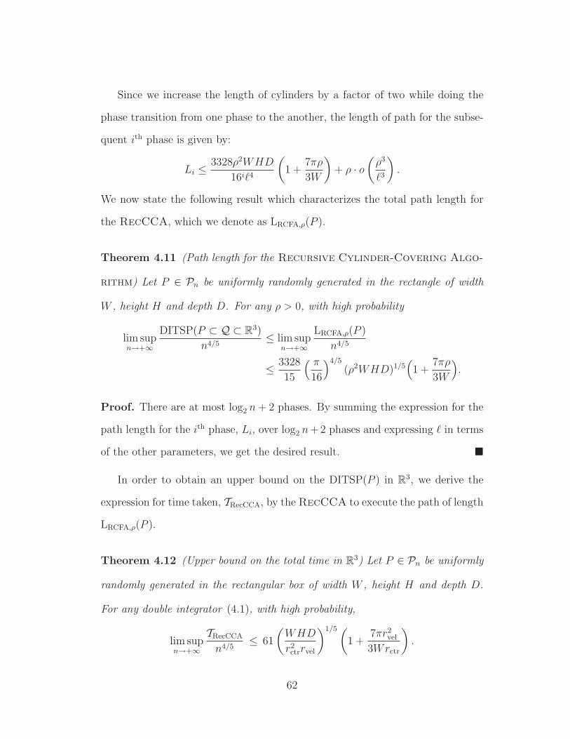
Since we increase the length of cylinders by a factor of two while doing the

phase transition from one phase to the another, the length of path for the subse-

quent ith phase is given by:

Li ≤3328ρ2WHD

16iℓ4

(1 +

7πρ

3W

)+ ρ · o

(ρ3

ℓ3

).

We now state the following result which characterizes the total path length for

the RecCCA, which we denote as LRCFA,ρ(P ).

Theorem 4.11 (Path length for the Recursive Cylinder-Covering Algo-

rithm) Let P ∈ Pn be uniformly randomly generated in the rectangle of width

W , height H and depth D. For any ρ > 0, with high probability

lim supn→+∞

DITSP(P ⊂ Q ⊂ R3)

n4/5≤ lim sup

n→+∞

LRCFA,ρ(P )

n4/5

≤ 3328

15

( π16

)4/5

(ρ2WHD)1/5(1 +

7πρ

3W

).

Proof. There are at most log2 n+ 2 phases. By summing the expression for the

path length for the ith phase, Li, over log2 n+2 phases and expressing ℓ in terms

of the other parameters, we get the desired result.

In order to obtain an upper bound on the DITSP(P ) in R3, we derive the

expression for time taken, TRecCCA, by the RecCCA to execute the path of length

LRCFA,ρ(P ).

Theorem 4.12 (Upper bound on the total time in R3) Let P ∈ Pn be uniformly

randomly generated in the rectangular box of width W , height H and depth D.

For any double integrator (4.1), with high probability,

lim supn→+∞

TRecCCA

n4/5≤ 61

(WHD

r2ctrrvel

)1/5(1 +

7πr2vel

3Wrctr

).

62

Proof. We substitute ρ =r2velrctr

in the bound for LRCFA,ρ(P ) given by Theorem 4.11

and evaluate the time required to traverse the total path of length LRCFA,ρ(P ) at

speed rvel.

Remark 4.13 Theorems 4.4 and 4.12 imply that, with high probability, the Rec-

CCA is a 50(1 +

7πr2vel3Wrctr

)-factor approximation (with respect to n) to the optimal

stochastic DITSP in R3 and that E[DITSP(P ⊂ Q ⊂ R

3)] belongs to Θ(n4/5).

4.3 The DTRP for double integrator

We now turn our attention to the Dynamic Traveling Repairperson Problem

(DTRP) for the double integrator modeled in eqn. (4.1). In the DTRP, the dou-

ble integrator is required to visit a dynamically growing set of targets, generated

by some stochastic process. We assume that the double integrator has unlimited

range and target-servicing capacity. We let D(t) denote the set of n(t) outstand-

ing target positions representing the demand at time t. Targets are generated

and inserted into D according to a time-invariant spatio-temporal Poisson pro-

cess with time intensity λ > 0 and with uniform spatial density inside the region

Q. As before, Q is a rectangle in two dimensions and a rectangular box in three

dimensions. Servicing of a target and its removal from the set D is achieved when

the double integrator moves to the target position. A control policy Φ for the

DTRP assigns a control input to the vehicle as a function of its configuration and

of the current outstanding targets. The policy Φ is a stable policy for the DTRP

if, under its action

nΦ = limt→+∞

E[n(t)| p = Φ(p,D)] < +∞,

63

i.e., if the double integrator is able to service targets at a rate that is, on average,

at least as large as the target generation rate λ. Let Tj be the time elapsed

from the time the jth target is generated to the time it is serviced and let TΦ :=

limj→+∞ E[Tj] be the steady-state system time for the DTRP under the policy

Φ. (If the system is stable, then it is known [45] that nΦ = λTΦ.)

In what follows, we design a control policy Φ whose system time TΦ is within

a constant-factor approximation of the optimal achievable performance. Consis-

tently with the theme of the chapter, we consider the case of heavy load, i.e., the

problem as the time intensity λ → +∞. We first provide lower bounds for the

system time, and then present novel approximation algorithms providing upper

bound on the performance.

Theorem 4.14 (Lower bound on the DTRP system time) For a double in-

tegrator (4.1), the system time TDTRP,2 and TDTRP,3 for the DTRP in two and

three dimensions satisfy

lim infλ→∞

TDTRP,2

λ2≥ 81

32

WH

rvelrctr, lim inf

λ→∞

TDTRP,3

λ4≥ 7813

972

WHD

rvelr2ctr

.

Proof. For a stable policy, the average time, t∗(n∗), needed to service a tar-

get must be no greater than the average time interval in which a new target is

generated, i.e., E[t∗(n∗)] ≤ 1/λ, where n∗ is the average number of outstanding

targets. This gives a bound on n∗. Using Little’s formula [45], one obtains the

result.

In Chapter 3, we proposed a simple strategy, the Bead-Tiling Algorithm

(BTA) for the DTRP for Dubins vehicle in R2. We adapt the BTA for the DTRP

problem for a double integrator in R2 and based on those ideas, we propose the

64

Cylinder Covering Algorithm (CCA) for R3. The BTA strategy consists

of the following steps:

(i) Tile the plane with beads of length ℓ := minCBTA/λ, 4ρ, where CBTA =

0.5241rvel

(1 + 7πρ

3W

)−1.

(ii) Traverse all non-empty beads once, visiting one target per bead. Repeat

this step.

The CCA strategy is akin to the BTA, where the region is covered with

cylinders constructed from beads of length ℓ := minCCFA/λ, 4ρ, where CCCA =

0.1615rvel

(1 + 7πρ

3W

)−1. The policy is then to traverse all non-empty cylinders

once, visiting one target per cylinder. The following result characterizes the

system time for the closed loop system induced by these algorithms and is based

on the bounds derived to arrive at Theorems 4.6 and 4.12.

Theorem 4.15 (Upper bound on the DTRP system time) For a double in-

tegrator (4.1) and λ > 0, the BTA and the CCA are stable policies for the DTRP

and the resulting system times TBTA and TCFA satisfy:

lim supλ→∞

TDTRP,2

λ2≤ lim sup

λ→∞

TBTA

λ2≤ 70.5

WH

rvelrctr

(1 +

7πr2vel

3Wrctr

)3

,

lim supλ→∞

TDTRP,3

λ4≤ lim sup

λ→∞

TCFA

λ4≤ 2 · 107 WHD

rvelr2ctr

(1+

7πr2vel

3rctr

)5

.

Proof. For the given policies, we derive bounds on the target generation rate

and servicing rate for a bead/cylinder. The bead/cylinder is then modeled as a

standard M/D/1 queue and we use the known result [45] for the system time for

such a queue.

65

Remark 4.16 Note that the achievable performances of the BTA and the CCA

provide a constant-factor approximation to the lower bounds established in The-

orem 4.14.

4.4 Extension to the TSPs for the Dubins vehi-

cle in R3

In Chapter 3, we have studied the Dubins Traveling Salesperson Problem

(DTSP) for the planar case. In that chapter, we proposed an algorithm that

gave a constant factor approximation to the optimal stochastic DTSP with high

probability. This naturally led to a stable policy for the DTRP problem for

the Dubins vehicle in R2 which also performed within a constant factor of the

optimal with high probability. The RecCCA developed in this chapter can

naturally be extended to apply to the stochastic DTSP in R3. It follows directly

from Lemma 4.5 that in order to use the RecCCA for a Dubins vehicle with

minimum turning radius ρ, one has to simply compute feasible curves for double

integrator moving with a constant speed√ρrctr. Hence the results stated in

Theorem 4.12 and Theorem 4.15 also hold true for the Dubins vehicle.

This equivalence between trajectories makes the RecCCA the first known

strategy with a strictly sub-linear asymptotic minimum time for the stochastic

DTSP in R3. Also novel is that the RecCCA performs within a constant factor

of the optimal with high probability and gives rise to a constant factor approxi-

mation and stabilizing policy for DTRP for Dubins vehicle in R3.

66

4.5 Summary

In this chapter we have proposed novel algorithms for various TSP problems

for vehicles with double integrator dynamics. We showed that the DITSP(P )

belongs to O(n1− 12d ) and in the worst case also belongs to Ω(n1− 1

d ). We fur-

ther proposed novel approximation algorithm and showed that the stochastic

DITSP(P ) belongs to Θ(n2/3) in R2 and to Θ(n4/5) in R

3, both with high proba-

bility. The policy proposed in this chapter for the DTRP for a double integrator

help in proving that the system time belongs to Θ(λ2) in R2 and to Θ(λ4) in R

3.

Comparing our results with those for the single integrator [24], we argue that our

analysis rigorously establishes the following intuitive fact: higher order dynamics

make the system much more sensitive to increases in the target generation rate.

It is interesting to note that the results presented in the chapter hold true

even in the presence of small damping in the double integrator dynamics: the

lower bounds are the same because the damping only slows down the vehicle; the

upper bounds also remain the same as long as the damping coefficient is relatively

small as compared to rctr.

67

Chapter 5

The coverage problem for

loitering Dubins vehicles

In this chapter we study a facility location problem for groups of Dubins

vehicles, i.e., nonholonomic vehicles that are constrained to move along planar

paths of bounded curvature, without reversing direction. Given a compact region

and a group of Dubins vehicles, the coverage problem is to minimize the worst-

case traveling time from any vehicle to any point in the region. Since the vehicles

cannot hover, we assume that they fly along static closed curves called loitering

curves. The chapter presents circular loitering patterns for a Dubins vehicle

and for a group of Dubins vehicles that minimize the worst-case traveling time

in sufficiently large regions. We do this by establishing an analogy to the disk

covering problem.

68

5.1 Problem Setup and notations

In this section we setup the main problem of the chapter and review some

basic required notation.

5.1.1 Dubins vehicle and feasible path

A Dubins vehicle is a planar vehicle that is constrained to move along paths

of bounded curvature, without reversing direction and maintaining a constant

speed. We will design loitering patterns for n Dubins vehicle in a compact re-

gion Q ⊂ R2, where R is the set of real numbers. Designing loitering patterns

encompasses deciding the distribution of vehicles into teams, specifying the loi-

tering curves for each team and the motion of vehicles along their respective

loitering curves. Given a duration T > 0, let γ : [0, T ] → R2 be a closed feasi-

ble curve for the Dubins vehicle or a closed Dubins path, i.e., γ is a curve that

is twice differentiable almost anywhere, ‖γ′(t)‖ = 1 for all t ∈ [0, T ], and the

magnitude of the curvature of γ is bounded above by 1/ρ, where ρ > 0 is the

minimum turning radius and γ(0) = γ(1). The configuration of the Dubins ve-

hicle traversing the curve γ(t) will be denoted by gγ(t) ∈ SE(2), where SE(2) is

the special Euclidean group of dimension 2, i.e., gγ(t) = (γ(t),ArcTan(γ′(t))).

Let the symbol I ∈ SE(2) represent the identity element of the SE(2) group.

Specifically, I will correspond to that state of the Dubins vehicle where it is po-

sitioned at the origin and its heading is aligned with the positive X axis. Let

Γρ = γ | γ is a closed Dubins path. The loitering curves that are designed in

this chapter belong to Γρ.

69

5.1.2 The coverage problem

Given n vehicles, a team composition can be represented as m1, . . . ,mn,

where mi ∈ N ∪ 0 and∑n

i=1mi = n. Here N represents the set of natural

numbers. In particular, if there are ℓ ≤ n teams, then the team composition will

be given by m1, . . . ,mℓ, 0, . . . , 0. Let M(n) denote the set of all such possible

team compositions. The idea is to partition Q into ℓ sub-regions such that each

team is responsible for one sub-region. Given ℓ teams, let Λ = (γ1, . . . , γℓ) ∈ Γℓρ

be a set of closed Dubins path for the teams. These curves will represent the

loitering curves for the Dubins vehicle. In this chapter we will be concerned

with minimizing the worst case traveling time to any arbitrary (unknown) target

point in Q by the closest Dubins vehicle. Since we constrain the vehicles to move

at constant (unit) speed along the curves, one can prove by symmetry that the

vehicles that are part of the same team are equally spaced along their common

loitering curve and move in the same direction (i.e., clockwise/counter-clockwise).

Therefore, given a region Q and a team composition M = (m1, . . . ,mℓ, 0, . . . , 0),

Λ completely specifies the loitering pattern.

We now define the coverage cost associated with a given loitering pattern.

Let Lρ : SE(2) × R2 → R≥0 be the length of the shortest Dubins path from

initial position and orientation, described by an element of SE(2), to a point

q ∈ R2, where R is the set of real numbers and R≥0 is the set of non-negative real

numbers. Recall that Lρ is continuous almost everywhere [46].

Definition 5.1 (Coverage cost) Given a region Q, a team composition M ,

and a loitering pattern Λ = (γ1, . . . , γℓ) with durations (T1, . . . , Tℓ), define the

70

coverage cost associated with the loitering pattern by

TQ,M(Λ) := supq∈Q

mini∈1,...,ℓ

sups∈[0,

Timi

)

minj∈1,...,mi

Lρ

(gγi

(s+

(j − 1)Timi

), q).

The coverage cost gives the worst-case traveling time from any vehicle to any

point in the region. In the rest of the chapter, we will use coverage cost and cost

interchangeably. The minimum cost associated with the given region Q and team

composition M is defined by

T ∗Q,M := inf

Λ∈Γℓρ

TQ,M(Λ).

In general, the optimal loitering patterns will have to be computed based on

the shape of the region Q. However, we will concentrate on circular loitering

patterns ; the rationale for doing so is that it (simplifies the problem and) allows

us to provide algorithms and bounds that are independent of the particular shape

of the environment. Furthermore, it seems unlikely that UAVs in the field will

be able to compute optimal loitering patterns as their assigned regions change

in real time; on the other hand, determining the location of the center, and the

radius of a circular loitering patterns are much easier tasks.

For a given center c ∈ R2, radius r > 0, let O(c, r) : [0, T ] → R

2 represent a

circle of radius r with center c. A complete specification of a circular loitering

curve would also involve specifying the direction of motion (i.e., clockwise or

counter-clockwise) for the vehicles along the circle. However, in our problem

setup, the coverage cost is not affected by the direction of motion as long as

all the vehicles along the same circular loitering curve have the same direction

of motion. Hence, we shall use O(c, r) along with an implicit and arbitrary

71

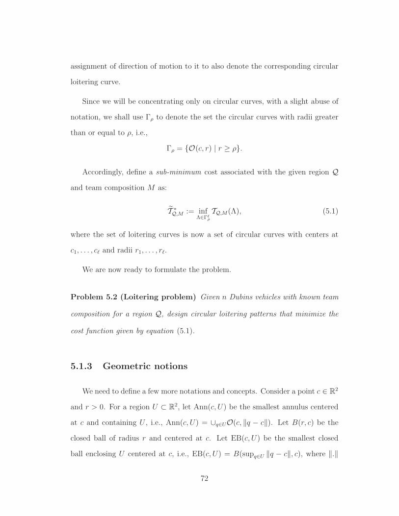
assignment of direction of motion to it to also denote the corresponding circular

loitering curve.

Since we will be concentrating only on circular curves, with a slight abuse of

notation, we shall use Γρ to denote the set the circular curves with radii greater

than or equal to ρ, i.e.,

Γρ = O(c, r) | r ≥ ρ.

Accordingly, define a sub-minimum cost associated with the given region Q

and team composition M as:

T ∗Q,M := inf

Λ∈Γℓρ

TQ,M(Λ), (5.1)

where the set of loitering curves is now a set of circular curves with centers at

c1, . . . , cℓ and radii r1, . . . , rℓ.

We are now ready to formulate the problem.

Problem 5.2 (Loitering problem) Given n Dubins vehicles with known team

composition for a region Q, design circular loitering patterns that minimize the

cost function given by equation (5.1).

5.1.3 Geometric notions

We need to define a few more notations and concepts. Consider a point c ∈ R2

and r > 0. For a region U ⊂ R2, let Ann(c, U) be the smallest annulus centered

at c and containing U , i.e., Ann(c, U) = ∪q∈UO(c, ‖q − c‖). Let B(r, c) be the

closed ball of radius r and centered at c. Let EB(c, U) be the smallest closed

ball enclosing U centered at c, i.e., EB(c, U) = B(supq∈U ‖q − c‖, c), where ‖.‖

72

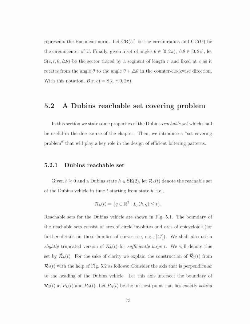
represents the Euclidean norm. Let CR(U) be the circumradius and CC(U) be

the circumcenter of U. Finally, given a set of angles θ ∈ [0, 2π), θ ∈ [0, 2π], let

S(c, r, θ,θ) be the sector traced by a segment of length r and fixed at c as it

rotates from the angle θ to the angle θ + θ in the counter-clockwise direction.

With this notation, B(r, c) = S(c, r, 0, 2π).

5.2 A Dubins reachable set covering problem

In this section we state some properties of the Dubins reachable set which shall

be useful in the due course of the chapter. Then, we introduce a “set covering

problem” that will play a key role in the design of efficient loitering patterns.

5.2.1 Dubins reachable set

Given t ≥ 0 and a Dubins state h ∈ SE(2), let Rh(t) denote the reachable set

of the Dubins vehicle in time t starting from state h, i.e.,

Rh(t) = q ∈ R2 | Lρ(h, q) ≤ t.

Reachable sets for the Dubins vehicle are shown in Fig. 5.1. The boundary of

the reachable sets consist of arcs of circle involutes and arcs of epicycloids (for

further details on these families of curves see, e.g., [47]). We shall also use a

slightly truncated version of Rh(t) for sufficiently large t. We will denote this

set by Rh(t). For the sake of clarity we explain the construction of RI(t) from

RI(t) with the help of Fig. 5.2 as follows: Consider the axis that is perpendicular

to the heading of the Dubins vehicle. Let this axis intersect the boundary of

RI(t) at PL(t) and PR(t). Let PB(t) be the furthest point that lies exactly behind

73

Figure 5.1: Reachable sets RI(t) for the Dubins vehicle for t = 3ρ, 5ρ and 7ρ.

the Dubins vehicle. Let HL(t) be the half-plane generated by the line passing

through PL(t) and PB(t) that does not contain the origin. Similarly, let HR(t) be

the half-plane generated by the line passing through PR(t) and PB(t) that does

not contain the origin. Then RI(t) = RI(t)\ (HL(t)∩HR(t)). It follows from the

above construction that Rh(t) is an inner approximation of RI(t). Moreover, as

observed in Figure 5.2, the approximation is fairly tight.

Using the definition of the reachable sets and planar geometry, one can prove

that the following properties hold true for any h ∈ SE(2).

(P1) Rh(t) is a monotonic function in t, i.e., Rh(t′) ⊆ Rh(t) for t′ ≤ t.

There exist constants κ1 ∈ [5.7, 5.8] and κ2 ∈ [6.5, 6.6] such that

(P2) Rh(t) is a simply connected set for all t ∈ R≥0 \ [κ1ρ, κ2ρ], and

74

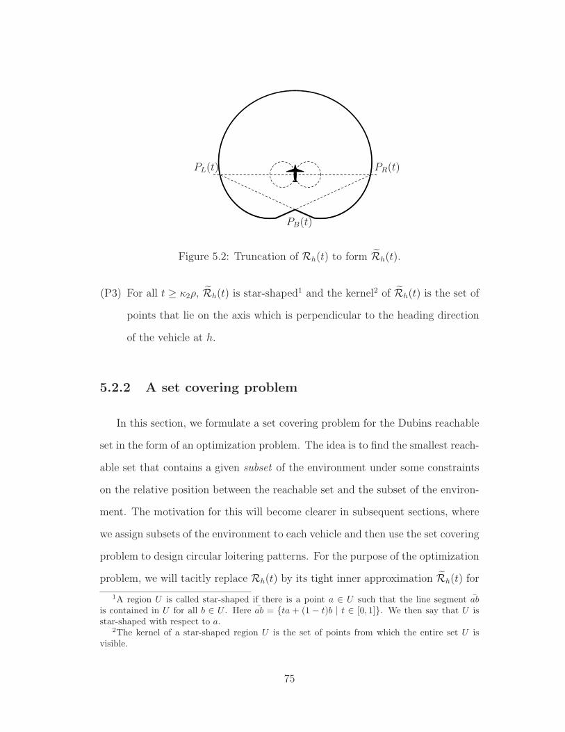
PB(t)

PL(t) PR(t)

Figure 5.2: Truncation of Rh(t) to form Rh(t).

(P3) For all t ≥ κ2ρ, Rh(t) is star-shaped1 and the kernel2 of Rh(t) is the set of

points that lie on the axis which is perpendicular to the heading direction

of the vehicle at h.

5.2.2 A set covering problem

In this section, we formulate a set covering problem for the Dubins reachable

set in the form of an optimization problem. The idea is to find the smallest reach-

able set that contains a given subset of the environment under some constraints

on the relative position between the reachable set and the subset of the environ-

ment. The motivation for this will become clearer in subsequent sections, where

we assign subsets of the environment to each vehicle and then use the set covering

problem to design circular loitering patterns. For the purpose of the optimization

problem, we will tacitly replace Rh(t) by its tight inner approximation Rh(t) for

1A region U is called star-shaped if there is a point a ∈ U such that the line segment ab

is contained in U for all b ∈ U . Here ab = ta + (1 − t)b | t ∈ [0, 1]. We then say that U isstar-shaped with respect to a.

2The kernel of a star-shaped region U is the set of points from which the entire set U isvisible.

75

t ≥ κ2ρ.

For a given positive integer m and t > 0, we state the following optimization

problem with variables r, λ and θ.

maximize r,

subj. to r > 0,

λ > ρ,

0 6 θ 6 2π,

S((0, λ), r, θ,

2π

m

)⊆ RI(t).

For a fixed m, we associate the solution of this optimization problem with

functions Rm,Λm,Θm : R≥0 → R≥0, m = 1, 2, . . ., which are defined so that(Rm(t),Λm(t),Θm(t)

)is the value of (r, λ, θ) at optimality for the above opti-

mization problem.

Geometrically, for a fixed m and t, a solution to the optimization problem

gives the specifications of the largest sector extending an angle 2πm

at the origin

such that it is contained inside RI(t) and its center lies on the Y axis and at

least at a distance of ρ from the origin. Specifically, the radius of such a sector is

given by Rm(t), its center is at Λm(t) and it is contained between the rays making

angles Θm(t) and Θm(t) + 2πm

with the X axis. In particular, R1(t) denotes the

radius of the largest disk contained inside RI(t) and whose center lies on the Y

axis and at least ρ distance from the origin.

One can show that, at fixed m, the function t 7→ Rm(t) is a strictly increasing

function in t. This is also illustrated in Figs. 5.6 and 5.7, where we have plotted

R1(t) vs. t and R2(t) vs. t respectively for ρ = 1. Hence, the inverse function

76

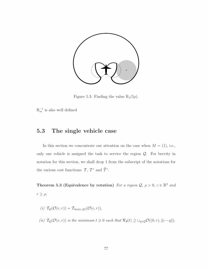
Figure 5.3: Finding the value R1(5ρ).

R−1m is also well defined

5.3 The single vehicle case

In this section we concentrate our attention on the case when M = (1), i.e.,

only one vehicle is assigned the task to service the region Q. For brevity in

notation for this section, we shall drop 1 from the subscript of the notations for

the various cost functions: T , T ∗ and T ∗.

Theorem 5.3 (Equivalence by rotation) For a region Q, ρ > 0, c ∈ R2 and

r ≥ ρ,

(i) TQ(O(c, r)) = TAnn(c,Q)(O(c, r)),

(ii) TQ(O(c, r)) is the minimum t > 0 such that RI(t) ⊇ ∪q∈QO((0, r), ‖c−q‖).

77

Figure 5.4: Finding the value R1(7ρ).

In addition, if TQ(O(c, r)) ∈ R≥0 \ [κ1ρ, κ2ρ], then

TQ(O(c, r)) = TEB(c,Q)(O(c, r)).

Proof. For brevity in notation, we let gO(c,r)(s) = g(s), i.e., g(s) represents the

generic state of the Dubins vehicle while moving along the circular curve O(c, r).

For a point q ∈ Q, define the function τ(q) = sups∈[0,T ) Lρ(g(s), q). This definition

implies that τ(q) is the minimum t such that q belongs to Rg(s)(t) for all s ∈ [0, T ).

Consider any other point q′ (not necessarily in Q) such that ‖q′ − c‖ = ‖q − c‖.

By rotational symmetry about the center c, given any s ∈ [0, T ), one can always

find a s′ ∈ [0, T ) such that Lρ(g(s′), q′) = Lρ(g(s), q), i.e., q′ also belongs to

Rg(s′)(τ(q)) for all s′ ∈ [0, T ). This implies that the circle of radius ‖c − q‖ and

centered at c belongs to Rg(s)(τ(q)) for all s ∈ [0, T ). Taking the union over

all q ∈ Q, one arrives at part (i) of the theorem. Let TQ(O(c, r)) = t∗. Part

(i) implies that ∪q∈QO(c, ‖c − q‖) belongs to Rg(s)(t∗) for all s ∈ [0, T ). This

property when viewed in the reference frame attached to the Dubins vehicle gives

78

Figure 5.5: Finding the value R4(7ρ).

8 9 10 11 12

5

6

7

8

t

R1(t)

Figure 5.6: Plot of R1(t) vs. t for ρ = 1.

the result in part (ii). This, combined with the simply connectedness property

(P2) of the reachable set implies that a disk of radius maxq∈Q ‖c− q‖ centered at

(0, r) belongs to RI(t∗) if t∗ ∈ R≥0 \ [κ1ρ, κ2ρ]. An equivalent statement is that

for values in R≥0 \ [κ1ρ, κ2ρ], t∗ is the smallest t such that EB(c,Q) ⊂ Rg(s)(t)

for all s ∈ [0, T ), that is, TEB(c,Q)(O(c, r)) = t∗ = TQ(O(c, r)).

We are now ready to state the main result of this section.

Theorem 5.4 (An optimal circular loitering curve) Given a region Q for

79

8 9 10 11 12

7

8

9

10

11

t

R2(t)

Figure 5.7: Plot of R2(t) vs. t for ρ = 1.

which CR(Q) ∈ R≥0 \ [R1(κ1ρ),R1(κ2ρ)], the circle of radius Λ1

(R−1

1 (CR(Q)))

with center at CC(Q) is an optimal circular loitering curve over Q, and the

corresponding coverage cost is given by

T ∗Q = R−1

1

(CR(Q)

).

Proof. We shall consider the case when CR(Q) ≥ κ2ρ. The proof for the

case when CR(Q) ≤ κ1ρ follows on similar lines. From the definition of R1,

CR(Q) ≥ κ2ρ implies that

mint ∈ R≥0 | B(CR(Q), (0, r)) ⊂ RI(t) ≥ κ2ρ.

Since CD(Q) is the minimum of all the enclosing balls of Q, we also have that

mint ∈ R≥0 | EB((0, r),REB(c,Q)) ⊂ RI(t) ≥ κ2ρ.

The closedness and the simply connectedness property of RI(t) for t ≥ κ2ρ implies

that

mint ∈ R≥0 | O((0, r),REB(c,Q)) ⊂ RI(t) ≥ κ2ρ.

This combined with Theorem 5.3 gives us that

TQ(O(c, r)) = mint ∈ R≥0 | ∪q∈Q O((0, r), ‖c− q‖) ⊂ RI(t) ≥ κ2ρ.

80

Since TQ(O(c, r)) ≥ κ2ρ, the previous discussion combined with Theorem 5.3

implies that

TQ(O(c, r)) = TEB(c,Q)(O(c, r)) ≥ TCD(Q)(O(CC(Q), r)).

This proves that the location of the center of rotation for an optimal circular

loitering curve is at the circumcenter of Q.

Therefore,

T ∗Q = min

c∈R2, r≥ρTQ(O(c, r))

= minr≥ρ

TCD(Q)(O(CC(Q), r))

= mint ∈ R≥0 | B(CR(Q), (0, r)) ⊂ RI(t) for some r ≥ ρ

= R−11 (CR(Q)).

The fact that Λ1

(R−1

1 (CR(Q)))

is the radius of an optimal circular loitering curve

follows from the definition of Λ1. This also proves the expression for the coverage

cost as stated in the theorem.

Remark 5.5 (Circular loitering patterns are optimal) Although we have been

restricting our attention on circular loitering curves, one can prove that, for the

single vehicle case, an optimal circular loitering curve is also an optimal loitering

curve, i.e.,

T ∗Q = T ∗

Q = R−11 (CR(Q)).

81

5.4 The single team case

In this section we design a loitering circle for a team of n Dubins vehicles

servicing the region Q, i.e., M = (n, 0, . . . , 0). For brevity in notation, we shall

denote this team composition by M = (n). By symmetry, the n vehicles will

be placed at an angular distance of 2πn

from each other. We now introduce the

concept of Dubins Voronoi Partition for vehicles moving along a circular loitering

curve O(c, r). Let g = g1, . . . , gn ∈ SE(2)n be a state of the n equally spaced

Dubins vehicles loitering along the curve O(c, r). We note here that, due to

the symmetrical placement of the vehicles along the loitering curve, the set g is

completely defined by specifying any one of its elements. We define the Dubins

Voronoi cell generated by gi by

V (gi, c, r, n) = q ∈ R2 | Lρ(gi, q) ≤ Lρ(gj, q) for all j ∈ 1, . . . , n.

Theorem 5.6 (Equivalence by rotation) For a region Q, ρ > 0, c ∈ R2,

r ≥ ρ and n > 1,

(i) TQ,n(O(c, r)) = TAnn(c,Q),n(O(c, r)),

(ii) Pick any h ∈ SE(2) along the circular loitering curve O(c, r). Then,

TQ,n(O(c, r)) is the minimum t > 0 such that Rh(t) ⊇ V (h, c, r, n) ∩

Ann(c,Q).

Proof. For the sake of this proof we will interpret TQ,1(O(c, r)) as the minimum

t for which Q belongs to ∪j∈1,...,nRgO(c,r)(s+(j−1)Tn

)(t) for all s ∈ [0, Tn). With

a slight abuse of notation, for the fixed circular loitering curve O(c, r), define

82

the function τ by τ(q) = Tq,n(O(c, r)). This definition implies that τ(q) is the

smallest t which satisfies the property that, given a s ∈ [0, Tn), there exists at

least one vehicle j ∈ 1, . . . , n such that q belongs to RgO(c,r)(s+(j−1)Tn

)(t). Con-

sider any other point q′ (not necessarily in Q) such that ‖q′ − c‖ = ‖q − c‖.

By rotational symmetry about the center c, one can find j′ ∈ 1, . . . , n such

that Lρ(gO(c,r)(s + (j′ − 1)Tn), q′) = Lρ(gO(c,r)(s + (j − 1)T

n), q), i.e., q′ also

belongs to ∪j∈1,...,nRgO(c,r)(s+(j−1)Tn

)(t). This implies that the circle of radius

‖c − q‖ and centered at c belongs to ∪j∈1,...,nRgO(c,r)(s+(j−1)Tn

)(t) for all s ∈

[0, Tn). Taking the union over all q ∈ Q, one arrives at the result in part (i).

TAnn(c,Q),n(O(c, r)) can be interpreted as the minimum t for which Ann(c,Q) be-

longs to ∪j∈1,...,nRgO(c,r)(s+(j−1)Tn

)(t) for all s ∈ [0, Tn). Part (ii) then follows from

the rotational symmetry about the center c and the definition of Dubins Voronoi

partition.

Theorem 5.6 suggests how to compute the optimal circular trajectory for a

team of Dubins vehicles by converting it into an optimization problem for a single

vehicle. However, solving this optimization problem requires the knowledge of

the shape of Dubins Voronoi partitions. Even though there is an element of

rotational symmetry in our case, the shapes of the Dubins Voronoi partition

(e.g., see Figure 5.8) are not easy enough to lend themselves to analysis. Hence,

we shall approximate the Voronoi partitions by sectors as shown in Figure 5.9.

This approximation helps in deriving upper bounds on the cost function.

We are now ready to state the main result of the section.

Theorem 5.7 (An upper bound on the coverage cost for a single team in large

environments) Given a region Q for which CR(Q) ≥ Rn(κ2ρ), the circle of radius

83

Figure 5.8: Dubins Voronoi partition for 4 vehicles loitering symmetrically along

a common circular curve.

Λn

(R−1n (CR(Q))

)with center at CC(Q) is an approximation to the optimal cir-

cular loitering curve over Q, and the corresponding upper bound on the coverage

cost is given by

T ∗Q,n ≤ R−1

n (CR(Q)).

Proof. Let T ∗Q,n = t∗. Similar to the proof of Theorem 5.4, one can show that

CR(Q) ≥ Rn(κ2ρ) implies that t∗ > κ2ρ. Theorem 5.6 implies that

t∗ = mint | V (gO(c,r)(s), c, r, n) ∩ Ann(c,Q) ⊂ RgO(c,r)(s)(t),

for any s ∈ [0, T ). Changing the reference frame to the one attached to the Dubins

vehicle and approximating the Dubins Voronoi partitions by sectors one can state

that t∗ is the minimum t such that S((0, r),REB(c,Q), α, 2π

n

)\S((0, r),minq∈Q ‖q−

c‖, α, 2πn

)⊂ RI(t) for any α ∈ [0, 2π). Since t∗ > κ2ρ, RI(t) is star-shaped and

84

Figure 5.9: Approximation of Dubins Voronoi partition by sectors.

simply connected for all t > t∗. Also RI(t) is an inner approximation of RI(t).

Combining these observations with the definition of R−1n , one arrives at the result.

Remark 5.8 The bound obtained in Theorem 5.7 is tightest among the bounds

possible by approximations of Dubins Voronoi partitions for vehicles moving along

circular curves by sectors of circles.

5.5 The multiple uniform team case

In this section we consider the multiple team case, concentrating on the case

when the teams have uniform composition. A group of n vehicles comprising of

ℓ teams is said to have uniform team composition if n is a multiple of ℓ and the

team composition is of the form (nl, . . . , n

l, 0, . . . , 0). We shall show that, for a

85

Figure 5.10: “Move-toward-the-circumcenter” algorithm for 16 disks in a convex

polygonal domain. The left (respectively, right) figure illustrates the initial (re-

spectively, final) locations and Voronoi partition. The central figure illustrates

the network evolution. After 20 sec., the disk radius is approximately 0.43273 m.

Simulations taken from [1].

sufficiently large and convex region Q, an upper bound on the cost of coverage

by the l team of loitering Dubins vehicles can be obtained by solving a related

disk covering problem.

We first briefly describe the disk-covering problem or, more precisely, the

version of the disk covering problem that is relevant for our purposes here. In

our context, the disk covering problem can be stated as follows: given a convex

region Q and an integer ℓ, find the smallest real number RDCQ(ℓ) and a set of

locations c1, . . . , cℓ such that the ℓ disks, each of radius RDCQ(ℓ) and centered

at c1, . . . , cℓ cover Q, that is, Q ⊂ ∪i∈1,...,ℓB(RDCQ(ℓ), ci). We shall refer to(RDCQ(ℓ), c1, . . . , cℓ

)as the solution to the disk covering problem for Q.

Disk covering problems have a long and beautiful history [48]. Many variants

of the problem (e.g., geometric minimum disk cover problem) find their applica-

tions in numerous engineering applications (e.g., localization in sensor networks).

In [1] distributed algorithms were designed to solve the disk covering problem

86

via a dynamical systems approach. Specifically, the chapter proposes the move

toward the furthest and move toward the circumcenter algorithms for a group of

ℓ mobile robots. In the move toward the furthest algorithm, each “disk center”

moves towards the furthest vertex of its Voronoi cell (inside the Voronoi par-

tition generated by all “disk centers”). In the ’move toward the circumcenter ’

algorithm, each disk-center moves toward the circumcenter of its Voronoi cell. In

both algorithms the Voronoi partition is continuously updated as the disk centers

move. Asymptotically, an execution of one of these two algorithms computes a

locally optimal solution to the disk covering problem in the sense that the lo-

cation of these robots correspond to the centers c1, . . . , cℓ and the largest of the

circumradii of the Voronoi partitions corresponds to RDCQ(ℓ). Moreover, these

distributed control laws can be implemented as local interactions between the disk

centers. In our setting, this would imply that this would require interaction only

between neighboring teams of vehicles, i.e., teams whose center of rotations are

Voronoi neighbors. An execution of the move toward the circumcenter algorithm

is illustrated in Figure 5.10.

We now state the following result which gives an upper bound on the coverage

cost for multiple uniform teams of loitering Dubins vehicles.

Theorem 5.9 Consider a group of n Dubins vehicles divided into ℓ teams of

uniform composition loitering in a convex region Q. Let(RDCQ(ℓ), c1, . . . , cℓ

)

be the solution to the disk covering problem for Q. If Area(Q) ≥ ℓπR2nℓ(κ2ρ),

then

T ∗Q,(n

ℓ,...,n

ℓ,0,...,0) ≤ R−1

nℓ

(RDCQ(ℓ)

).

Moreover, the loitering pattern which achieves this upper bound is the set of circu-

87

lar curves, each of radius Λnℓ

(R−1

nℓ

(RDCQ(ℓ)

)), and with centers at c1, . . . , cℓ.

Using the control algorithms from [1], one can design a computational approach

to computing loitering patterns as follows:

(i) Partition the environment into Voronoi partitions generated by virtual cen-

ters.

(ii) Move the virtual centers in such a way as to solve a minimum-radius disk-

covering problem

(iii) Designing efficient loitering patterns for each team in its corresponding

Voronoi cell.

5.6 Summary

In this chapter, we considered the coverage problem for loitering Dubins vehi-

cles. We have characterized the configuration of the vehicles at the appearance of

new targets in terms of Dubins paths, that we call loitering patterns. We defined

the coverage cost to be the worst-case traveling time from any vehicle to any point

in the region. Optimal circular loitering for a single vehicle and efficient circular

loitering for a single team of vehicles were characterized. Finally, by establishing

an analogy to the disk-covering problem, we proposed a computational approach

to characterize efficient loitering patterns for multiple uniform teams.

This chapter leaves numerous important extensions open for further research.

One needs to study the functions R−1n to derive closed form expression for the

bounds derived in this chapter. It would be interesting to consider the coverage

88

problem for other meaningful cost functions. The problem of multi non-uniform

team of vehicles is also important. Determining the ideal team composition for

a given region provides an exciting challenge too.

89

Chapter 6

Maintaining limited-range

connectivity among second-order

agents

In this chapter we consider ad-hoc networks of agents with double integrator

dynamics. For such networks, the connectivity maintenance problems are: (i) do

there exist control inputs for each agent to maintain network connectivity, and (ii)

given desired controls for each agent, can one compute the closest connectivity-

maintaining controls in a distributed fashion? The proposed solution is based on

three contributions. First, we define and characterize admissible sets for double

integrators to remain inside disks. Second, we establish an existence theorem for

the connectivity maintenance problem by introducing a novel state-dependent

graph, called the double-integrator disk graph. Finally, we design a distributed

“flow-control” algorithm to compute optimal connectivity-maintaining controls.

90

6.1 Preliminary developments

We begin with some notations. We let N, N0, and R+ denote the natural

numbers, the non-negative integer numbers, and the positive real numbers, re-

spectively. For d ∈ N, we let 0d and 1d denote the vectors in Rd whose entries

are all 0 and 1, respectively. We let ‖p‖ denote the Euclidean norm of p ∈ Rd.

For r ∈ R+ and p ∈ Rd, we let B(p, r) denote the closed ball centered at p with

radius r, i.e., B(p, r) = q ∈ Rd | ‖p−q‖ ≤ r. For x, y ∈ R

d, we let x y denote

component-wise inequality, i.e., xk ≤ yk for k ∈ 1, . . . , d. We let f : A B

denote a set-valued map; in other words, for each a ∈ A, f(a) is a subset of B.

We identify Rd × R

d with R2d.

6.1.1 Maintaining a double integrator inside a disk

For t ∈ N0, consider the discrete-time control system in R2d

p[t+ 1] = p[t] + v[t],

v[t+ 1] = v[t] + u[t],

(6.1)

where the norm of the control is upper-bounded by rctr ∈ R+, i.e., u[t] ∈

B(0d, rctr) for t ∈ N0. We refer to this control system as the discrete-time double

integrator in Rd or, more loosely, as a second-order system. Given (p, v) ∈ R

2d

and uττ∈N0 ⊆ B(0d, rctr), let φ(t, (p, v), uτ) denote the solution of (6.1) at

time t ∈ N0 from initial condition (p, v) with inputs u1, . . . , ut−1.

In what follows we consider the following problem: assume that the initial

position of (6.1) is inside a disk centered at 0d, find inputs that keep it inside

that disk. This task is impossible for general values of the initial velocity. In

91

what follows we identify assumptions on the initial velocity that render the task

possible.

For rpos ∈ R+, we define the admissible set at time zero by

Ad0(rpos) = B(0d, rpos) × R

d.

For rpos, rctr ∈ R+, we define the admissible set for m time steps by

Adm(rpos, rctr) =

(p, v) ∈ R

2d | ∃uττ∈[0,m−1] ⊆ B(0d, rctr)

s.t. φ(t, (p, v), uτ) ∈ Ad0(rpos) ∀t ∈ [0,m]

,

and the admissible set by

Ad(rpos, rctr) =(p, v) ∈ R

2d | ∃uττ∈N0 ⊆ B(0d, rctr)

s.t. φ(t, (p, v), uτ) ∈ Ad0(rpos), ∀t ∈ N0

.

With slight abuse of notation we shall sometimes suppress the arguments in the

definitions of admissible sets. The following theorem establishes some important

properties of the admissible sets.

Theorem 6.1 (Properties of the admissible sets) For all d ∈ N and rpos, rctr ∈

R+, the following statements hold:

(i) for all m ∈ N, Adm(rpos, rctr) ⊆ Ad

m−1(rpos, rctr) and

Ad(rpos, rctr) = limm→+∞

Adm(rpos, rctr) = lim

m→+∞∩mk=1 Ad

k(rpos, rctr) ;

(ii) Ad(rpos, rctr) is a convex, compact set and is the largest controlled-invariant1

subset of Ad0(rpos);

1A set is controlled invariant for a control system if there exists a feedback law such that the

set is positively invariant for the closed-loop system.

92

(iii) Ad(rpos, rctr) is invariant under orthogonal transformations in the sense

that, if (p, v) ∈ Ad(rpos, rctr), then also (Rp,Rv) ∈ Ad(rpos, rctr) for all

orthogonal2 matrices R in Rd×d;

(iv) if 0 < r1 < r2, then Ad(rpos, r1) ⊂ Ad(rpos, r2) and Ad(r1, rctr) ⊂ Ad(r2, rctr).

Proof. The two facts in statement (i) are direct consequences of the definitions of

Adm and Ad. Regarding statement (ii), each Ad

m, m ∈ N, is closed, the intersection

of closed sets is closed, and, therefore, Ad = limm→+∞ ∩mk=1 Adk is closed. To show

that Ad is bounded it suffices to show that Ad1 is bounded. Note that (p, v) ∈ Ad

1

implies that there exists u ∈ B(0d, rctr) such that (p, v) ∈ Ad0 and (p+ v, v+u) ∈

Ad0. This, in turn, implies that p ∈ B(0d, rpos) and p+ v ∈ B(0d, rpos). Therefore,

Ad1 is bounded. Next, we prove that Ad

m is convex. Given (p1, v1) and (p2, v2) in

Adm, let u1 and u2 be controls that ensure that φ(t, (pi, vi), ui) ∈ Ad

0, t ∈ [0,m],

i ∈ 1, 2. For λ ∈ [0, 1], consider the initial condition (pλ, vλ) = (λp1 + (1 −

λ)p2, λv1 + (1 − λ)v2) and the input uλ = λu1 + (1 − λ)u2, and note that, by

linearity,

φ(t, (pλ, vλ), uλ) = λφ(t, (p1, v1), u1) + (1 − λ)φ(t, (p2, v2), u2), t ∈ [0,m].

Because φ(t, (p1, v1), u1) and φ(t, (p2, v2), u2) belong to the convex set Ad0,

then also their convex combination does. Therefore, (pλ, vλ) belongs to Adm, and

Adm is convex. Finally, Ad is convex because the intersection of convex sets is

convex.

Next, we show that Ad is controlled invariant. Given (p, v) ∈ Ad (with corre-

sponding control sequence uττ∈N0), we need to show that there exists a control

2A matrix R ∈ Rd×d is orthogonal if RRT = RT R = Id.

93

input x ∈ B(0d, rctr) such that φ(1, (p, v), x) ∈ Ad. Such input can be chosen as

x = u0. Indeed, the control sequence uτ+1τ∈N0 keeps the trajectory starting

from φ(1, (p, v), x) inside Ad0 and, therefore, φ(1, (p, v), x) ∈ Ad. Additionally, it

is easy to see that Ad ⊂ Ad0. Finally, we need to prove that Ad is the largest

controlled-invariant subset of Ad0. Assume that there exists Ad∗ with the same

properties and larger than Ad. This means that there exists (p, v) ∈ Ad∗ \ Ad.

This is equivalent to saying that ∃ τ ∗ ∈ N0 such that, for every choice of the

input u, φ(τ ∗, (p, v), u) /∈ Ad0. But, since Ad∗ ⊂ Ad

0, this leads to a contradiction.

Regarding statement (iii), observe that, if (p, v) ∈ Ad0, then (Rp,Rv) ∈ Ad

0

and, if u ∈ B(0, rctr), then Ru ∈ B(0, rctr). Therefore, using again the linearity

of the maps φ, the proof follows. Regarding statement (iv), the two results

follow from the definition of Ad(rpos, rctr) and the facts that, for all 0 < r1 < r2,

B(0, r1) ⊂ B(0, r2) and Ad0(r1) ⊂ Ad

0(r2).

Next, we study the set-valued map that associates to each state in Ad(rpos, rctr)

the set of control inputs that keep the state inside Ad(rpos, rctr) in one step. We

define the admissible control set Ud(rpos, rctr) : Ad(rpos, rctr) B(0d, rctr) by

Ud(rpos, rctr) · (p, v) = u ∈ B(0d, rctr) | (p+ v, v + u) ∈ Ad(rpos, rctr),

or, equivalently,

Ud(rpos, rctr) · (p, v) = B(0d, rctr)∩w − v | (p+ v, w) ∈ Ad(rpos, rctr). (6.2)

Lemma 6.2 (Properties of the admissible control set)

For all (p, v) ∈ Ad(rpos, rctr), the set Ud(rpos, rctr) · (p, v) is non-empty, convex

and compact. For generic (p, v) ∈ Ad(rpos, rctr), the set Ud(rpos, rctr) · (p, v) does

not contain 0d.

94

Proof. The non-emptiness of the set Ud(rpos, rctr) · (p, v) derives directly from

the definition of Ad(rpos, rctr). Clearly, from equation (6.2), Ud(rpos, rctr) · (p, v) is

closed (it is the intersection of two closed sets). It is also bounded (Ud(rpos, rctr) ·

(p, v) ⊂ B(0d, rctr)), hence it is compact. To prove that it is convex, we need

to show the following: given (p, v) ∈ Ad(rpos, rctr), if there exist u1 and u2 in

Ud(rpos, rctr) · (p, v) such that φ(1, (p, v), u1) and φ(1, (p, v), u2) belong to

Ad(rpos, rctr), then u12 = λu1+(1−λ)u2, λ ∈ [0, 1], belongs to Ud(rpos, rctr)·(p, v),

that is, φ(1, (p, v), u12) ∈ Ad(rpos, rctr). But this fact follows directly from the

linearity of φ and the convexity of Ad(rpos, rctr). This proves that Ud(rpos, rctr) ·

(p, v) is convex. The fact that it does not necessarily contain the origin can be

proven by contradiction as follows. Consider a (p, v) ∈ Ad(rpos, rctr) such that

v 6= 0d and Ud(rpos, rctr)·(p, v) contains 0d. This means that (p+v, v) also belongs

to Ad(rpos, rctr). Now, either Ud(rpos, rctr) · (p+v, v) does not contain 0d, in which

case we have proved the statement, or Ad(rpos, rctr) also contains (p + 2v, v).

Continuing along these lines, if it were true that Ud(rpos, rctr) · (p, v) contains the

origin for all (p, v) ∈ Ad(rpos, rctr), then one could show that (p + tv, v) belongs

to Ad(rpos, rctr) for all t ∈ N. However, Ad(rpos, rctr) is bounded by Theorem 6.1.

Hence, one can always find a t∗ ∈ N such that (p + t∗v, v) ∈ Ad(rpos, rctr) but

(p + (t∗ + 1)v, v) /∈ Ad(rpos, rctr), thereby proving that Ud(rpos, rctr) · (p + t∗v, v)

does not contain 0d.

6.1.2 Computing admissible sets

We characterize Ad for d = 1 in the following result and we illustrate the

outcome in Figure 6.1.

95

Lemma 6.3 (Admissible set in 1 dimension) For rpos, rctr ∈ R+, the fol-

lowing holds:

(i) A1(rpos, rctr) is the polytope containing the points (p, v) ∈ R2 satisfying

−rpos

m− m− 1

2rctr ≤ v +

p

m≤ rpos

m+m− 1

2rctr, (6.3)

for all m ∈ N, and p ∈ [−rpos, rpos];

(ii) If m(rpos, rctr) ∈ N is defined by

m(rpos, rctr) =

⌈−1

2+

√1

4+

4rpos

rctr

⌉, (6.4)

then A1 = A1m = A1

bm(rpos,rctr), for m ≥ m(rpos, rctr).

Proof. Regarding statement (i), it suffices to show that, for m ∈ N, A1m(rpos, rctr)

is the set of points in A1m−1(rpos, rctr) that satisfy equation (6.3). If we show that

this property holds for all m, then we can use statement (i) of Theorem 6.1 to

complete the proof. Consider the set of equations (6.1) for m consecutive time

indices after t. The solution of the linear system can be written in terms of the

state at instant t asp[t+m]

v[t+m]

=

1 m

0 1

p[t]

v[t]

+

m−1∑

τ=0

1 (m− 1 − τ)

0 1

0

1

u[t+ τ ], (6.5)

where we used the equality

Aτ =

1 1

0 1

τ

=

1 τ

0 1

, τ ∈ N.

It is clear that the points on the boundary of A1m have the property that the

maximum control effort is needed to enforce the constraint. In other words we

96

look for the points (p[t], v[t]) ∈ A10 with v[t] ≥ 0 (the case v[t] ≤ 0 can be solved

in a similar way) such that the points p[t +m] ≤ rcmm are reached by using the

maximum control effort u[t+ τ ] = −rctr, τ ∈ 0, . . . ,m− 1.

Substituting the expression of the control in (6.5) we obtain

p[t+m] = p[t] +mv[t] − rctr

m−1∑

τ=0

(m− 1 − τ),

v[t+m] = v[t] −mrctr,

and using the equality∑m−1

τ=0 (m− 1 − τ) = m(m−1)2

, we have

p[t+m] = p[t] +mv[t] − rctrm(m− 1)

2,

v[t+m] = v[t] −mrctr,

(6.6)

In order to belong to A1m, the point (p[t], v[t]) must satisfy the constraint p[t+τ ] ≤

rcmm, τ ∈ 1, . . . ,m, or equivalently

v[t] ≤ −p[t]τ

+rcmm

τ+ rctr

(τ − 1)

2, τ ∈ 1, . . . ,m.

Using the same procedure for the points in the half plane v[t] ≤ 0 (in this case

the control is u[t + τ ] = rctr, τ ∈ 0, . . . ,m − 1), it turns out that A1m is equal

to the set of all pairs (p, v) ∈ A10 satisfying

−pτ− rcmm

τ− τ − 1

2rctr ≤ v ≤ −p

τ+rcmm

τ+τ − 1

2rctr, τ ∈ 1, . . . ,m.

By using statement (i) of Theorem 6.1 the proof is complete.

Regarding statement (ii), let us consider the case v[t] ≥ 0 and evaluate the

points on the boundary such that (p[t+m], v[t+m]) = (rcmm, 0), m ∈ N. These

points are obtained by substituting the above value of (p[t+m], v[t+m]) in (6.6).

The points obtained are (p, v) such that

p = rcmm −m(m+ 1)

2rctr, m ∈ N0.

97

It is easy to see that m(rpos, rctr), as defined in equation (6.4), is the lowest m

such that p ≤ −rcmm.

Remarks 6.4 (i) If rctr ≥ 2rpos, then A1 = A11, that is, for sufficiently large

rctr/rpos, the admissible set is equal to the admissible set in 1 time step.

(ii) The methodology for constructing A1(rpos, rctr) is related to the procedure

for constructing the so-called isochronic regions for discrete time optimal

control of double integrators, as outlined in [49].

Next, we introduce some definitions useful to provide an inner approximation

of Ad when d ≥ 2. Given p ∈ Rd and v ∈ R

d \ 0d, define p‖ ∈ R and p⊥ ∈ Rd

by

p = p‖v

‖v‖ + p⊥,

where p⊥ · v = 0. For rpos, rctr ∈ R+, define

Ad‖(rpos, rctr) =

(p, v) ∈ B(0d, rpos) × R

d | v = 0d or

(p‖, ‖v‖) ∈ A1(√

r2pos − ‖p⊥‖2, rctr

). (6.7)

Lemma 6.5 For rpos, rctr ∈ R+, Ad‖(rpos, rctr) is a compact subset of Ad(rpos, rctr).

Proof. We begin by showing that definition (6.7) is equivalent to

Ad‖(rpos, rctr) =

(p, v) ∈ Ad

0 | v = 0d or ∃u‖ττ∈N0 ⊆ [−rctr, rctr]

s.t. φ(t, (p, v), u‖τ

v

‖v‖)∈ Ad

0(rpos), ∀t ∈ N0

. (6.8)

98

p

v

m=

1

m=

1

m=

2

m=

2m = 3

m = 3

−rpos

rpos

Figure 6.1: The admissible set A1 for generic values of rpos and rctr

To establish this equivalence, we use the definition of the set A1. For v 6= 0d, we

rewrite the solution of the system as

φ(t, (p, v), uτ) = φ‖(t, (p, v), uτ)v

‖v‖ + φ⊥(t, (p, v), uτ),

where φ⊥(t, (p, v), uτ) · v = 0 for all t ∈ N0. It is easy to see that, if uττ∈N0 =

u‖ττ∈N0

v‖v‖ , then φ⊥(t, (p, v), uτ) = (p⊥, 0d) for all t ∈ N0. Therefore,

φ(t, (p, v), uτ) = φ‖(t, (p, v), uτ)v

‖v‖ + (p⊥, 0d).

Note that, if p = p‖v

‖v‖ + p⊥, then ‖p‖ ≤ rpos if and only if p‖ ≤√r2pos − ‖p⊥‖2.

Therefore, the property φ(t, (p, v), u‖τ v

‖v‖

)∈ Ad

0(rpos) is equivalent to

φ‖(t, (p, v), u‖τ

v

‖v‖)∈ A1

0

(√r2pos − ‖p⊥‖2

),

and, in turn, definitions (6.7) and (6.8) are equivalent. In order to prove that

Ad‖(rpos, rctr) is compact, we simply observe that it is a closed subset of the com-

pact set Ad(rpos, rctr).

99

Remark 6.6 In what follows we use our representation of Ad‖ to compute an

inner approximation for the convex set Ad, for d ≥ 2. For example, for fixed

p ∈ B(0d, rpos), we compute velocity vectors v such that (p, v) ∈ Ad by considering

a sample of unit-length vectors w ∈ Rd and computing the maximum allowable

velocity v parallel to w according to equation (6.7). Furthermore, we perform

computations by adopting inner polytopic representations for the various compact

convex sets.

6.1.3 The double-integrator disk graph

Let us introduce some concepts about state dependent graphs and some useful

examples. For a set X, let F(X) be the collection of finite subsets of X; e.g.,

P ∈ F(Rd) is a set of points. For a finite set X, let G(X) be the set of undirected

graphs whose vertices are elements of X, i.e., whose vertex set belongs to F(X).

For a set X, a state dependent graph on X is a map G : F(X) → G(X) that

associates to a finite subset V of X an undirected graph with vertex set V and

edge set EG(V ) where EG : F(X) → F(X ×X) satisfies EG(V ) ⊆ V × V . In other

words, what edges exist in G(V ) depends on the elements of V that constitute

the nodes.

The following three examples of state dependent graphs play an important

role. First, given rpos ∈ R+, the disk graph Gdisk(rpos) is the state dependent

graph on Rd defined as follows: for p1, . . . , pn ⊂ R

d, the pair (pi, pj) is an edge

in Gdisk(rpos) · (p1, . . . , pn) if and only if

‖pi − pj‖ ≤ rpos ⇐⇒ pi − pj ∈ B(0d, rpos).

100

Second, given rpos, rctr ∈ R+, the double-integrator disk graph Gdi-disk(rpos, rctr) is

the state dependent graph on R2d defined as follows: for (p1, v1), . . . , (pn, vn) ⊂

R2d, the pair ((pi, vi), (pj, vj)) is an edge if and only if the relative positions and

velocities satisfy

(pi − pj, vi − vj) ∈ Ad(rpos, rctr).

Third, it is convenient to define the disk graph also as a state dependent graph

on R2d by stating that ((pi, vi), (pj, vj)) is an edge if and only if (pi, pj) is an edge

of the disk graph on Rd. We illustrate the first two graphs in Figure 6.2.

Remark 6.7 As is well known, the disk graph is invariant under rigid trans-

formations and reflections. Loosely speaking, the double integrator disk graph is

invariant under the following class of transformations: position and velocities of

the agents may be expressed with respect to any rotated and translated frame that

is moving at constant linear velocity. These transformations are related to the

classic Galilean transformations in geometric mechanics.

6.2 Connectivity constraints among second-order

agents

In this section we state the model, the notion of connectivity, and a sufficient

condition that guarantees connectivity can be preserved.

101

Figure 6.2: The disk graph and the double-integrator disk graph in R2 for 20

agents with random positions and velocities.

6.2.1 Networks of robotic agents with second-order dy-

namics and the connectivity maintenance problem

We begin by introducing the notion of network of robotic agents with second-

order dynamics in Rd. Let n be the number of agents. Each agent has the

following computation, motion control, and communication capabilities. For i ∈

1, . . . , n, the ith agent has a processor with the ability of allocating continuous

and discrete states and performing operations on them. The ith agent occupies

a location pi ∈ Rd, moves with velocity vi ∈ R

d, according to the discrete-time

double integrator dynamics in (6.1), i.e.,

pi[t+ 1] = pi[t] + vi[t],

vi[t+ 1] = vi[t] + ui[t],

(6.9)

where the norm of all controls ui[t], i ∈ 1, . . . , n, t ∈ N0, is upper-bounded by

rctr ∈ R+. The communication model is the following. The processor of each

agent has access to the agent location and velocity. Each agent can transmit

information to other agents within a distance rcmm ∈ R+. We remark that the

102

control bound rctr and the communication radius rcmm are the same for all agents.

Remarks 6.8 (i) Our network model assumes synchronous execution, although

it would be important to consider more general asynchronous networks.

(ii) We will not address here the correctness of our algorithms in the presence

of measurement errors or communication quantization.

We now state the control design problem of interest.

Problem 6.9 (Connectivity Maintenance) Choose a state dependent graph

Gtarget on R2d and design (state dependent) control constraints sets with the fol-

lowing property: if each agent’s control takes values in the control constraint set,

then the agents move in such a way that the number of connected components of

Gtarget (evaluated at the agents’ states) does not increase with time.

This objective is to be achieved with the limited information available through

message exchanges between agents. This problem was originally stated and solved

for first-order agents in [33].

6.2.2 A known result for agents with first-order dynamics

In [33], a connectivity constraint was developed for a set of agents modeled

by first-order discrete-time dynamics:

pi[t+ 1] = pi[t] + ui[t].

Here the graph whose connectivity is of interest, is the disk graph Gdisk(rcmm) over

the vertices p1[t], . . . , pn[t]. Network connectivity is maintained by restricting

103

the allowable motion of each agent. In particular, it suffices to restrict the motion

of each agent as follows. If agents i and j are neighbors in the rcmm-disk graph

Gdisk(rcmm) at time t, then their positions at time t+ 1 are required to belong to

B(pi[t]+pj [t]

2, rcmm

2

). In other words, connectivity between i and j is maintained if

ui[t] ∈ B(pj[t] − pi[t]

2,rcmm

2

),

uj[t] ∈ B(pi[t] − pj[t]

2,rcmm

2

).

The constraint is illustrated in Figure 6.3.

Note that this constraint takes into account only the positions of the agents;

this fact can be attributed to the first-order dynamics of the agents. We wish

to construct a similar constraint for agents with second order dynamics. It is

reasonable to expect that this new constraint will depend on positions as well as

velocities of the neighboring agents.

pj

pi

Figure 6.3: Starting from pi and pj, the agents are restricted to move inside the

disk centered atpi+pj

2with radius rcmm

2.

104

6.2.3 An appropriate graph for the connectivity mainte-

nance problem for agents with second-order dynam-

ics

We begin working on the stated problem with a negative result regarding two

candidate target graphs.

Lemma 6.10 (Unsuitable graphs) Consider a network of n agents with dou-

ble integrator dynamics (6.9) in Rd. Let rcmm be the communication range and let

rctr be the control bound. Let Gtarget be either Gdisk(rcmm) on R2d or Gdi-disk(rcmm, 2rctr).

There exist states (pi, vi)i∈1,...,n such that

(i) the graph Gtarget at (pi, vi)i∈1,...,n is connected, and

(ii) for all uii∈1,...,n ⊆ B(0d, rctr), the graph Gtarget at (pi+vi, vi+ui)i∈1,...,n,

is disconnected.

Proof. The proof of the statement for Gtarget = Gdisk(rcmm) is straightforward.

Consider two agents whose relative position and velocity belong to Ad0\Ad

1. Then,

after one time step, the two agents will not be connected in Gdisk(rcmm) no matter

what their controls are. Next, consider the case Gtarget = Gdi-disk(rcmm, 2rctr).

For d = 1, let v be the maximal velocity in A1(rcmm, 2rctr) at p = 0, that is,

v = minrcmm/m+ (m− 1)rctr | m ∈ N. Take three agents with positions p1 =

p2 = p3 = 0 and velocities v1 = −v, v2 = 0, and v3 = v. At this configuration,

the graph Gdi-disk(rcmm, 2rctr) contains two edges: between agent 1 and 2 and

between agent 2 and 3. Connectivity is preserved after one time step if agent 2

105

remains connected to both agents 1 and 3 after one time step. However, to remain

connected with agent 1, its control u2 must be equal to −rctr and, analogously,

to remain connected with agent 3, its control u2 must be equal to +rctr. Clearly

this is impossible.

Remarks 6.11 (i) The result in Lemma 6.10 on the double integrator graph

has the following interpretation. Assume that agent i has two neighbors j

and k in the graph Gdi-disk(rcmm, rctr). By definition of the neighboring law

for this graph, we know that there exists bounded controls for i and j to

maintain the ((pi, vi), (pj, vj)) link and that there exists bounded controls

for i and k to maintain the ((pi, vi), (pk, vk)) link. The lemma states that,

for some states of the agents i, j, and k, there might not exist controls that

maintain both links simultaneously.

(ii) In other words, Lemma 6.10 shows how the disk graph Gdisk(rcmm) and the

double integrator disk graph Gdi-disk(rcmm, 2rctr) are not appropriate choices

for the connectivity maintenance problem.

The following theorem suggests that an appropriate scaling of the control

bound is helpful in identifying a suitable state dependent graph for Problem 6.9.

Theorem 6.12 (A scaled double-integrator disk graph is suitable) Consider

a network of n agents with double integrator dynamics (6.9) in Rd. Let rcmm be

the communication range and let rctr be the control bound. For k ∈ 1, . . . , n−1,

define

ν(k) =2

k√d.

106

Assume that k ∈ 1, . . . , n − 1 and the state (pi, vi)i∈1,...,n together have

the property that the graph Gdi-disk(rcmm, ν(k)rctr) at (pi, vi)i∈1,...,n contains

a spanning tree T with diameter at most k. Then there exists uii∈1,...,n ⊆

B(0d, rctr) such that if ((pi, vi), (pj, vj)) is an edge of T , then ((pi+vi, vi+ui), (pj+

vj, vj + uj)) is an edge of Gdi-disk(rcmm, ν(k)rctr) at (pi + vi, vi + ui)i∈1,...,n.

These results are based upon Shostak’s Theory for systems of inequalities, as

discussed in [50]. We provide the proof in Appendix C. The following results are

immediate consequences of this theorem.

Corollary 6.13 (Simple sufficient condition) With the same notation in The-

orem 6.12, define νmin = 2(n−1)

√d. Assume that the state (pi, vi)i∈1,...,n has the

property that the graph Gdi-disk(rcmm, νminrctr) is connected at (pi, vi)i∈1,...,n.

Then

(i) there exists uii∈1,...,n ⊆ B(0d, rctr), such that the graph

Gdi-disk(rcmm, νminrctr) is also connected at (pi + vi, vi + ui)i∈1,...,n; and

(ii) if T is a spanning tree of Gdi-disk(rcmm, νminrctr) at (pi, vi)i∈1,...,n, then

there exists uii∈1,...,n ⊆ B(0d, rctr), such that, for all edges ((pi, vi), (pj, vj))

of T , it holds that ((pi + vi, vi + ui), (pj + vj, vj + uj)) is an edge of

Gdi-disk(rcmm, νminrctr) at (pi + vi, vi + ui)i∈1,...,n.

Remark 6.14 (Scaling of νmin with n) The condition νmin = 2√d(n−1)

implies

that according to the sufficient conditions in Corollary 6.13, as the number of

107

agents grows, the velocities of the agents must be closer and closer in order for

the agents to be able to remain connected.

If Gdi-disk(rcmm, ν(k)rctr) at (pi, vi)i∈1,...,n is not connected for some k, then

Theorem 6.12 applies to its connected components. In what follows we fix k and

without loss of generality assume the graph Gdi-disk(rcmm, ν(k)rctr) at (pi, vi)i∈1,...,n

to be connected.

Remark 6.15 (Distributed computation of connectivity and of spanning trees)

Each agent can compute its neighbors in the graph Gdi-disk(rcmm, ν(k)rctr) just

by communicating with its neighbors in Gdisk(rcmm) and exchanging with them

position and velocity information. Alternatively, this computation may also be

performed if each agent may sense relative position and velocity with all other

agents at a distance no larger than rcmm.

It is possible to compute spanning trees in networks via standard depth-first

search distributed algorithms. It is also possible [51] to distributively compute a

minimum diameter spanning tree in a network.

6.2.4 The control constraint set and its polytopic repre-

sentation

We now concentrate on two agents with indices i and j. For t ∈ N0, we define

the relative position, velocity and control by pij[t] = pi[t]−pj[t], vij[t] = vi[t]−vj[t]

108

and uij[t] = ui[t] − uj[t], respectively. It is easy to see that

pij[t+ 1] = pij[t] + vij[t],

vij[t+ 1] = vij[t] + uij[t].

Assume that agents i, j are connected in Gdi-disk(rcmm, ν(k)rctr) at time t. By defi-

nition, this means that the relative state (pij[t], vij[t]) belongs to Ad(rcmm, ν(k)rctr).

If this connection is to be maintained at time t + 1, then the relative control at

time t must satisfy

ui[t] − uj[t] ∈ Ud(rcmm, ν(k)rctr) · (pij[t], vij[t]). (6.10)

Also, implicit are the following bounds on individual control inputs ui[t] and uj[t]:

ui[t] ∈ B(0d, rctr), uj[t] ∈ B(0d, rctr). (6.11)

This discussion motivates the following definition.

Definition 6.16 Given rcmm, rctr, ν(k) ∈ R+ and given a set E of edges in

Gdi-disk(rcmm, ν(k)rctr) at (pi, vi)i∈1,...,n, the control constraint set is defined by

UdE(rcmm, rctr, ν(k)) · (pi, vii∈1,...,n)

= (u1, . . . , un) ∈ B(0d, rctr)n | ∀((pi, vi), (pj, vj)) ∈ E,

ui − uj ∈ Ud(rcmm, ν(k)rctr) · (pi − pj, vi − vj).

In other words, the control constraint set for an edge set E is the set of

controls for each agent with the property that all edges in E will be maintained

in one time step.

Remark 6.17 We can now interpret the results in Theorem 6.12 as follows.

109

(i) To maintain connectivity between any pair of connected agents, we should

simultaneously handle constraints corresponding to all edges of

Gdi-disk(rcmm, ν(k)rctr). This might render the control constraint set empty.

(ii) However, if we only consider constraints corresponding to edges belonging to

a spanning tree T of Gdi-disk(rcmm, ν(k)rctr), then the set UdT (rcmm, ν(k)rctr) ·

(pi, vii∈1,...,n) is guaranteed to be nonempty.

Let us now provide a concrete representation of the control constraint set.

Given a pair i, j of connected agents, the admissible control set Ud(rcmm, ν(k)rctr)·

(pij, vij) is convex and compact (Lemma 6.2). Hence, we can fit a polytope with

Npoly sides inside it. This approximating polytope leads to the following tighter

version of the constraint in (6.10):

(Cηij)

T (ui − uj) ≤ wηij, η ∈ 1, . . . , Npoly, (6.12)

for some appropriate vector Cηij ∈ R

d and scalar wηij ∈ R. Similarly, one can

compute an inner polytopic approximation of the closed ball B(0d, rctr) and write

the following linear vector inequalities:

(Cηiθ)

Tui ≤ wηiθ, η ∈ 1, . . . , Npoly, (6.13)

where the symbol θ has the interpretation of a fictional agent. In this way, we

have cast the original problem of finding a set of feasible control inputs into a

satisfiability problem for a set of linear inequalities.

Remark 6.18 Rather than a network-wide control constraint set, one might like

to obtain decoupled constraint sets for each individual agent. However, (1) it is

110

not clear how to design a distributed algorithm to perform this computation, (2)

such an algorithm will likely have large communication requirements, and (3) such

a calculation might lead to a very conservative estimate for the decoupled control

constraint sets. Therefore, rather than explicitly decoupling the control constraint

sets, we next focus on a distributed algorithm to search the control constraint set

for feasible controls that are optimal according to some criterion.

6.3 Distributed computation of optimal controls

In this section we formulate and solve the following optimization problem:

given an array of desired control inputs Udes = (udes,1, . . . , udes,n)T ∈ (Rd)n, find,

via local computation, the array U = (u1, . . . , un) belonging to the control con-

straint set, that is closest to the desired array Udes. To formulate this problem

precisely, we need some additional notations. Let E be a set of edges in the

undirected graph Gdi-disk(rcmm, ν(k)rctr) at (pi, vi)i∈1,...,n. To deal with the

linear inequalities of the form (6.12) and (6.13) associated to each edge of E,

we introduce an appropriate multigraph. A multigraph (or multiple edge graph)

is, roughly speaking, a graph with multiple edges between the same vertices.

More formally, a multigraph is a pair (Vmult, Emult), where Vmult is the vertex

set and the edge set Emult contains numbered edges of the form (i, j, η), for

i, j ∈ V and η ∈ N, and where Emult has the property that if (i, j, η) ∈ Emult

and η > 1, then also (i, j, η − 1) ∈ Emult. In what follows, we let Gmult denote

the multigraph with vertex set 1, . . . , n and with edge set Emult = (i, j, η) ∈

1, . . . , n2 × 1, . . . , Npoly | ((pi, vi), (pj, vj)) ∈ E, i > j. Note that to each

element (i, j, η) ∈ Emult is associated the inequality (Cηij)

T (ui − uj) ≤ wηij. We

111

are now ready to formally state the optimization problem at hand in the form of

the following quadratic programming problem:

minimize1

2

n∑

i=1

‖ui − udes,i‖2,

subj. to (Cηij)

T (ui − uj) ≤ wηij, for (i, j, η) ∈ Emult,

(Cηiθ)

Tui ≤ wηiθ, for i ∈ 1, . . . , n, η ∈ 1, . . . , Npoly.

(6.14)

Here, somehow arbitrarily, we have adopted the 2-norm to define the cost func-

tion.

Remark 6.19 (Feasibility) If E is a spanning tree of Gdi-disk(rcmm, νrctr) at a

connected configuration (pi, vi)i∈1,...,n, then the control constraint set

UdE(rcmm, rctr, ν(k)) · (pi, vii∈1,...,n) is guaranteed to be non-empty by Theo-

rem 6.12. In turn, this implies that the optimization problem (6.14) is feasible.

6.3.1 Solution via duality: the projected Jacobi method

The problem (6.14) can be written in a compact form as:

minimize1

2‖U − Udes‖2,

subj. to BTmultU w,

for appropriately defined matrix Bmult and vector w. A dual “projected Ja-

cobi method” algorithm for the solution of this standard quadratic program is

described in Appendix B. According to this algorithm, let λ∗ be the value of

Lagrange multipliers at optimality. Then the global minimum for U is achieved

at

U∗ = Udes −Bmultλ∗. (6.15)

112

The projected Jacobi iteration for each component of λ is given by

λα(t+ 1) = max

0, λα(t) −τ

(BTmultBmult)αα

((w −BT

multUdes)α

+

Npoly(e+n)∑

β=1

(BTmultBmult)αβλβ(t)

), (6.16)

where α ∈ 1, . . . , Npoly(e + n) and τ is the step size parameter. We can select

τ = 1Npoly(e+n)

to guarantee convergence.

6.3.2 A distributed implementation of the dual algorithm

Because of the particular structure of the matrixBTmultBmult, the iterations (6.16)

can be implemented in a distributed way over the original graph G. To highlight

the distributed structure of the iteration we denote the components of λ by re-

ferring to the nodes that they share and the inequality they are related to. In

particular for each edge in Gmult, the corresponding Lagrange multiplier will be

denoted as ληij if the edge goes from node i to node j, i > j, and the edge is

associated to the inequality constraint Cηij(ui − uj) ≤ wηij. This makes up the

first Npolye entries of the vector λ. To be consistent with this notation, the next

Npolyn entries will be denoted λ11θ, . . . , λ

Npoly

1θ , . . . , λ1nθ, . . . , λ

Npoly

nθ . Additionally,

define N (i) = j ∈ 1, . . . , n | (pi, vi), (pj, vj) ∈ E ∪ θ. The symbol θ has

the interpretation of a fictional node.

Defining ληij := ληji and Cηij := −Cη

ji for i < j, we can write equations (6.15)

and (6.16) in components as follows. Equation (6.15) reads, for i ∈ 1, . . . , n,

u∗i = udes,i −∑

k∈N (i)

Npoly∑

η=1

Cηikλ

ηik.

113

One can easily work an explicit expression for the matrix product BTmultBmult

in (6.16). Then, equation (6.16) reads, for (i, j, η) ∈ Emult,

ληij(t+ 1) = max

0, ληij(t) −

τ

2(Cηij)

TCηij

·∑

k∈N (i)

Npoly∑

σ=1

((Cη

ij)TCσ

ikλσik

)+∑

k∈N (j)

Npoly∑

σ=1

((Cη

ji)TCσ

jkλσjk

)

+ wηij − (Cηij)

T (udes,i − udes,j)

,

together with, for i ∈ 1, . . . , n, η ∈ 1, . . . , Npoly,

ληiθ(t+ 1) = max

0, ληiθ(t)

− τ

(Cηiθ)

TCηiθ

( ∑

k∈N (i)

Npoly∑

σ=1

((Cηiθ)

TCσikλ

σik) + wηiθ − (Cη

iθ)Tudes,i

).

We distribute the task of running iterations for these Npoly(e + n) Lagrange

multipliers among the n agents as follows: an agent i carries out the updates

for all quantities ληiθ and all ληij for which i > j. By means of this partition

and by means of iterated one-hop communication among agents, it is possible to

compute the global solution for the optimization problem (6.14) in a distributed

fashion over the double integrator disk graph.

6.4 Simulations

To illustrate our analysis we focus on the following scenario. For the two

dimensional setting, i.e., for d = 2, we assume that there are n = 5 agents with

(randomly chosen) initial condition and such that they are connected according

114

to Gdi-disk. The bound for the control input is rctr = 2 and the communication

radius is rcmm = 10.

We assigned to one of the agents a derivative feedback control ux[p, v] =

(vx − 2), uy[p, v] = (vy − 5) as desired input. For the other agents the desired

input is set to zero. We show the agent trajectories in Figure 6.4a, the velocities of

the agents with respect to time in Figure 6.4b, and the distances between agents

which are neighbors in the spanning tree in Figure 6.4c. Notice that the agents

move with approximately identical velocity reaching a configuration in which

all of them are at the limit distance rcmm = 10. The interesting aspect of this

simulation is that the maintenance of connectivity leads to the accomplishment of

apparently unrelated coordination tasks as velocity alignment and cohesiveness.

This numerical result illustrate how our connectivity maintenance approach might

indeed be a starting point for novel investigations into the problem of flocking

with connectivity.

6.5 Summary

We provided some distributed algorithms to enforce connectivity among net-

works of agents with double-integrator dynamics. Future directions of research

include (i) evaluating the communication complexity of the proposed distributed

dual algorithm and possibly designing faster ones, (ii) studying the relationship

between the connectivity maintenance problem and the platooning and mesh

stability problem, and (iii) investigating the flocking phenomenon and designing

flocking algorithms which do not rely on a blanket assumption of connectivity.

115

0 50 100 150−10

0

10

20

30

40

50

60

70

pxi

pyi

(a) Positions

0 5 10 15 20 25 30 35−1

0

1

2

3

4

5

6

t

v i

(b) Velocities (vx and vy)

0 5 10 15 20 25 30 351

2

3

4

5

6

7

8

9

10

t

r ij

(c) Inter-agent distances

Figure 6.4: Velocity alignment and cohesiveness for 5 agents in the plane (d = 2)

116

Chapter 7

Conclusions

In the context of DTSP, future directions of research include finding a single

algorithm which would provide constant factor approximation to the DTSP for

the worst case as well as the stochastic setting. It is also interesting to consider

the non-uniform stochastic DTSP when the points to be serviced are sampled

according to a non-uniform probability distribution. Other avenues of future

research are to use the tools developed in this dissertation to study Traveling

Salesperson Problems for other dynamical vehicles, study decentralized versions

of the DTRP and general task assignment and surveillance problems for multi-

Dubins (and other dynamical) vehicles. Another set of interesting problems arise

when the environment is non-convex (e.g., environment with obstacles) and/or we

consider TSP problems without target location information, i.e., search problems.

Another variation of the problems to be considered is when vehicles have finite

servicing footprints.

An immediate extension of the results for the coverage problem would be to

117

consider teams with non-uniform team composition. Studying loitering patterns

with different notions of cost functions, like average cost instead of the worst-case

cost, would also be interesting. Designing loitering patterns over more general

class of curves (instead of only circular curves) is also a possible avenue of future

research.

The connectivity maintenance problem also gives rise to many other exciting

problems. An immediate task would be to evaluate the communication com-

plexity of the proposed distributed dual algorithm and possibly designing faster

ones. It would be interesting to study the relationship between the connectivity

maintenance problem and the platooning and mesh stability problem. It is also

interesting to investigate the flocking phenomenon and designing flocking algo-

rithms which do not rely on a blanket assumption of connectivity. Finally, it

would be exciting to extend this framework to more general notions of connec-

tivity.

In this dissertation, we dealt mainly with the motion coordination aspects of

multi-UAV systems. One can envision future UAV systems equipped with het-

erogeneous sensors like radars, acoustic transducers and collectively performing

various cooperative tasks like target identification, estimation and tracking. The

possibility to control sensor modalities (e.g., waveform selection, beam steering)

and mobility of sensor platforms (UAVs) gives the possibility to increase the per-

formance of conventional systems by orders of magnitude. At the same time, it

gives rise to challenging problems in sensor management, distributed estimation

and signal processing, data fusion and decentralized motion planning. Solving

these fundamental scientific problems is essential to extract the maximum out of

the emergent UAV technology.

118

Bibliography

[1] J. Cortes and F. Bullo, “Coordination and geometric optimization via dis-

tributed dynamical systems,” SIAM Journal on Control and Optimization,

vol. 44, no. 5, pp. 1543–1574, 2005.

[2] K. B. Ariyur, P. Lommel, and D. F. Enns, “Reactive inflight obstacle avoid-

ance via radar feedback,” in American Control Conference, (Portland, OR),

pp. 2978–2982, 2005.

[3] C. Tomlin, I. Mitchell, and R. Ghosh, “Safety verification of conflict reso-

lution manoeuvres,” IEEE Transactions on Intelligent Transportation Sys-

tems, vol. 2, no. 2, pp. 110–120, 2001.

[4] S. M. LaValle, Planning Algorithms. Cambridge, UK: Cambridge University

Press, 2006.

[5] U. Boscain and B. Piccoli, Optimal Syntheses for Control Systems on 2-

D Manifolds. Mathematiques et Applications, New York: Springer Verlag,

2004.

[6] P. R. Chandler, M. Pachter, D. Swaroop, J. M. Fowler, J. K. Howlett, S. Ras-

mussen, C. Schumacher, and K. Nygard, “Complexity in UAV cooperative

119

control,” in American Control Conference, (Anchorage, AK), pp. 1831–1836,

2002.

[7] Z. Tang and U. Ozguner, “Motion planning for multi-target surveillance

with mobile sensor agents,” IEEE Transactions on Robotics, vol. 21, no. 5,

pp. 898–908, 2005.

[8] R. W. Beard, T. W. McLain, M. A. Goodrich, and E. P. Anderson, “Coor-

dinated target assignment and intercept for unmanned air vehicles,” IEEE

Transactions on Robotics and Automation, vol. 18, no. 6, pp. 911–922, 2002.

[9] S. Rathinam, R. Sengupta, and S. Darbha, “A resource allocation algorithm

for multi-vehicle systems with non holonomic constraints,” IEEE Transac-

tions on Automation Sciences and Engineering, vol. 4, no. 1, pp. 98–104,

2007.

[10] E. Frazzoli and F. Bullo, “Decentralized algorithms for vehicle routing in

a stochastic time-varying environment,” in IEEE Conf. on Decision and

Control, (Paradise Island, Bahamas), pp. 3357–3363, Dec. 2004.

[11] A. E. Gil, S. Ganapathy, K. M. Passino, and A. Sparks, “Cooperative

scheduling of tasks for networked uninhabited autonomous vehicles,” in

IEEE Conf. on Decision and Control, (Maui, Hawaii), pp. 522–527, Dec.

2003.

[12] A. Richards, J. Bellingham, M. Tillerson, and J. How, “Coordination and

control of multiple UAVs,” in AIAA Conf. on Guidance, Navigation and

Control, (Monterey, CA), Aug. 2002.

120

[13] A. A. Markov, “Some examples of the solution of a special kind problem in

greatest and least quantities,” Soobshch. Kharkovsk. Mat. Obshch., vol. 1,

pp. 250–276, 1887. (in Russian).

[14] L. E. Dubins, “On curves of minimal length with a constraint on average

curvature and with prescribed initial and terminal positions and tangents,”

American Journal of Mathematics, vol. 79, pp. 497–516, 1957.

[15] J.-D. Boissonnat, A. Cerezo, and J. Leblond, “Shortest paths of bounded

curvature in the plane,” Journal of Intelligent and Robotic Systems, vol. 11,

pp. 5–20, 1994.

[16] A. M. Shkel and V. J. Lumelsky, “Classification of the Dubins set,” Robotics

and Autonomous Systems, vol. 34, pp. 179–202, 2001.

[17] J.-D. Boissonnat and S. Lazard, “A polynomial-time algorithm for com-

puting a shortest path of bounded curvature amidst moderate obstacles,”

International Journal of Computational Geometry & Applications, vol. 13,

pp. 189–229, 2003.

[18] J. Beardwood, J. Halton, and J. Hammersly, “The shortest path through

many points,” in Proceedings of the Cambridge Philosophy Society, vol. 55,

pp. 299–327, 1959.

[19] J. M. Steele, “Probabilistic and worst case analyses of classical problems of

combinatorial optimization in Euclidean space,” Mathematics of Operations

Research, vol. 15, no. 4, p. 749, 1990.

[20] D. Applegate, R. Bixby, V. Chvatal, and W. Cook, “On the solution of travel-

ing salesman problems,” in Documenta Mathematica, Journal der Deutschen

121

Mathematiker-Vereinigung, (Berlin, Germany), pp. 645–656, Aug. 1998. Pro-

ceedings of the International Congress of Mathematicians, Extra Volume

ICM III.

[21] S. Arora, “Nearly linear time approximation scheme for Euclidean TSP and

other geometric problems,” in IEEE Symposium on Foundations of Com-

puter Science, (Miami Beach, FL), pp. 554–563, Oct. 1997.

[22] S. Lin and B. W. Kernighan, “An effective heuristic algorithm for the

traveling-salesman problem,” Operations Research, vol. 21, pp. 498–516,

1973.

[23] A. Aggarwal, D. Coppersmith, S. Khanna, R. Motwani, and B. Schieber,

“The angular-metric traveling salesman problem,” SIAM Journal on Com-

puting, vol. 29, no. 3, pp. 697–711, 1999.

[24] D. J. Bertsimas and G. J. van Ryzin, “A stochastic and dynamic vehicle rout-

ing problem in the Euclidean plane,” Operations Research, vol. 39, pp. 601–

615, 1991.

[25] K. Savla, E. Frazzoli, and F. Bullo, “On the point-to-point and traveling

salesperson problems for Dubins’ vehicle,” in American Control Conference,

(Portland, OR), pp. 786–791, June 2005.

[26] J. Le Ny and E. Feron, “An approximation algorithm for the curvature-

constrained traveling salesman problem,” in Allerton Conference on Com-

munications, Control and Computing, (Monticello, IL), Sept. 2005.

[27] S. Darbha, “Combinatorial motion planning for a collection of Reeds-Shepp

vehicles,” tech. rep., ASEE/AFOSR SFFP, AFRL, Eglin, Aug. 2005.

122

[28] K. Savla, F. Bullo, and E. Frazzoli, “On traveling salesperson problems for

Dubins’ vehicle: stochastic and dynamic environments,” in IEEE Conf. on

Decision and Control and European Control Conference, (Seville, Spain),

pp. 4530–4535, Dec. 2005.

[29] S. Itani and M. A. Dahleh, “On the average length of the stochastic TSP with

Dubins’ metric,” tech. rep., LIDS, Massachusetts Institute of Technology,

2005.

[30] K. Savla, E. Frazzoli, and F. Bullo, “On the Dubins Traveling Sales-

person Problems: Novel approximation algorithms,” in Robotics: Sci-

ence and Systems II (Proceedings of the Second RSS Conference, August

2006, Philadelphia PA) (G. S. Sukhatme, S. Schaal, W. Burgard, and

D. Fox, eds.), Cambridge, MA: MIT Press, 2007. Available electronically

at http://arxiv.org/abs/cs.RO/0603010.

[31] C. Schumacher, P. R. Chandler, S. J. Rasmussen, and D. Walker, “Task

allocation for wide area search munitions with variable path length,” in

American Control Conference, (Denver, CO), pp. 3472–3477, 2003.

[32] J. Cortes, S. Martınez, T. Karatas, and F. Bullo, “Coverage control for

mobile sensing networks,” IEEE Transactions on Robotics and Automation,

vol. 20, no. 2, pp. 243–255, 2004.

[33] H. Ando, Y. Oasa, I. Suzuki, and M. Yamashita, “Distributed memoryless

point convergence algorithm for mobile robots with limited visibility,” IEEE

Transactions on Robotics and Automation, vol. 15, no. 5, pp. 818–828, 1999.

[34] J. Lin, A. S. Morse, and B. D. O. Anderson, “The multi-agent rendezvous

123

problem,” in IEEE Conf. on Decision and Control, (Maui, HI), pp. 1508–

1513, Dec. 2003.

[35] J. Cortes, S. Martınez, and F. Bullo, “Robust rendezvous for mobile au-

tonomous agents via proximity graphs in arbitrary dimensions,” IEEE

Transactions on Automatic Control, vol. 51, no. 8, pp. 1289–1298, 2006.

[36] A. Ganguli, J. Cortes, and F. Bullo, “On rendezvous for visually-guided

agents in a nonconvex polygon,” in IEEE Conf. on Decision and Control and

European Control Conference, (Seville, Spain), pp. 5686–5691, Dec. 2005.

[37] D. P. Spanos and R. M. Murray, “Motion planning with wireless network

constraints,” in American Control Conference, (Portland, OR), pp. 87–92,

June 2005.

[38] M. M. Zavlanos and G. J. Pappas, “Controlling connectivity of dynamic

graphs,” in IEEE Conf. on Decision and Control and European Control Con-

ference, (Seville, Spain), pp. 6388–6393, Dec. 2005.

[39] G. Percus and O. C. Martin, “Finite size and dimensional dependence of

the Euclidean traveling salesman problem,” Physical Review Letters, vol. 76,

no. 8, pp. 1188–1191, 1996.

[40] J. J. Enright and E. Frazzoli, “UAV routing in a stochastic time-varying

environment,” in IFAC World Congress, (Prague, Czech Republic), July

2005. Electronic Proceedings.

[41] R. Motwani and P. Raghavan, Randomized Algorithms. Cambridge, UK:

Cambridge University Press, 1995.

124

[42] Y. Azar, A. Z. Broder, A. R. Karlin, and E. Upfal, “Balanced allocations,”

SIAM Journal on Computing, vol. 29, no. 1, pp. 180–200, 1999.

[43] W. Feller, An Introduction to Probability Theory and Its Applications, vol. 1.

New York: John Wiley, 1968.

[44] J. M. Steele, Probability Theory and Combinatorial Optimization. Philadel-

phia, PA: SIAM, 1987.

[45] L. Kleinrock, Queueing Systems. Volume I: Theory. New York: John Wiley,

1975.

[46] J. J. Enright, E. Frazzoli, K. Savla, and F. Bullo, “On multiple UAV rout-

ing with stochastic targets: performance bounds and algorithms,” in AIAA

Conf. on Guidance, Navigation and Control, Aug. 2005. Electronic Proceed-

ings.

[47] J. Lawrence, A catalog of special plane curves. New York: Dover Publica-

tions, 1972.

[48] R. Kershner, “The number of circles covering a set,” American Journal of

Mathematics, vol. 61, no. 3, pp. 665–671, 1939.

[49] Z. Gao, “On discrete time optimal control: A closed-form solution,” in Amer-

ican Control Conference, (Boston, MA), pp. 52–58, 2004.

[50] B. Aspvall and Y. Shiloach, “A polynomial time algorithm for solving sys-

tems of linear inequalities with two variables per inequality,” SIAM Journal

on Computing, vol. 9, no. 4, pp. 827–845, 1980.

125

[51] M. Bui, F. Butelle, and C. Lavault, “A distributed algorithm for constructing

a minimum diameter spanning tree,” Journal of Parallel and Distributed

Computing, vol. 64, pp. 571–577, 2004.

[52] D. P. Bertsekas and J. N. Tsitsiklis, Parallel and Distributed Computation:

Numerical Methods. Belmont, MA: Athena Scientific, 1997.

126

Appendix A

On the proof of Theorem 2.4

A.1 Dubins classification of optimal curves

Following [14], the minimum length feasible curve for the Dubins vehicle is

either (i) an arc of a circle of radius ρ, followed by a line segment, followed by an

arc of a circle of radius ρ, or (ii) a sequence of three arcs of circles of radius ρ,

or (iii) a subpath of a path of path type (i) or (ii). To specify the type of these

minimum length feasible curves for the Dubins path we follow the notations used

in [16]. Three elementary motions are considered: turning to the left, turning

to the right (both along a circle of radius ρ), and straight line motion S. Three

operators are introduced: Lv (for left/counterclockwise turn of length v > 0),

Rv (for right/clockwise turn of length v > 0), Sv (for straight motion of length

v > 0). The operators Lv, Rv, and Sv, transform an arbitrary configuration

127

(x, y, ψ) ∈ SE(2) into its corresponding image point in SE(2) by

(x+ sin(ψ + v) − sinψ, y − cos(ψ + v) + cosψ, ψ + v),

(x− sin(ψ − v) + sinψ, y + cos(ψ − v) − cosψ, ψ − v),

(x+ v cosψ, y + v sinψ, ψ),

respectively. Thus, the Dubins set D which is the domain for the type of the

minimum length feasible curve for a Dubins vehicle between a given initial and

final configuration is given by D = LSL,RSR,RSL,LSR,RLR,LRL. One

may refer to [14] for a detailed discussion on the construction of these path types

between a given initial and final configuration. One may note that there are sets

of initial and final configurations for which all the path types may not be feasible

between those configurations.

In the remaining part of the chapter we will need to frequently use the curves

of type LRL and RLR starting with the initial configuration (0, 0, 0) and the

final configuration (0, 0, ψ). We introduce some additional notations to facilitate

presentation of the same. We introduce notations for the path type LRL. For

ψ 6= 0, let Cp1(ψ) be a circle with center OCp1:= (0, ρ) and radius ρ, and let

Cp2(ψ) be a circle with center OCp2:= (−ρ sinψ, ρ cosψ) and radius ρ. Note that

ψ 6= 0 implies that Cp1(ψ)∩Cp2(ψ) is either a point or 2 points. Then let Cm1(ψ)

and Cm2(ψ) be two circles with radius ρ that are tangent to both Cp1(ψ) and

Cp2(ψ), see Figure A.1 and Figure A.2.

By construction, Cp1(ψ) intersects Cm1(ψ) and Cm2(ψ) at one point each: let

P1(ψ) be the first of these two points that is reached moving left from the origin O

along Cp1(ψ). Without loss of generality, assume P1(ψ) ∈ Cm1(ψ). Let OCm1be

the center of Cm1 . Let P2(ψ) = Cm1(ψ) ∩ Cp2(ψ). In order to remove ambiguity,

128

δ

φ

ρ

O

ρ

Y

X

OCp2

OCm2

OCm1

OCp1

Cp2

Cm1

Cp1

P1

Cm2

ρ

ρ

P2ψ

Figure A.1: LRL curves returning to

the origin for ψ ∈ [0, π].

ρ

Y

X

OCp1

Cp1

Oψ

Cm2

Cp2

Cm1

OCp2

δ

φOCm1

ρOCm2

P1

P2

ρ

ρ

Figure A.2: LRL curves returning to

the origin for ψ ∈ (π, 2π).

we shall pick that heading of the tangent line to a circle at a given point which is

consistent with the orientation of that circle to be the orientation of the tangent to

that circle at that point. Let the orientation of the Dubins vehicle at P1 be along

the orientation of the tangent to Cp1 at P1. Similarly, let the orientation of the

Dubins vehicle at P2 be along the orientation of the tangent to Cp2 at P2. Let the

vehicle configuration at P1 and P2 be denoted by Jp1 , Jp2 ∈ SE(2), respectively.

Let t1, t2, t3 be such that Lt1(0, 0, 0) = Jp1 , Rt2(Jp1) = Jp2 and Lt3(Jp2) = (0, 0, ψ).

Let LRLO(ψ) and RLRO(ψ) be the minimum length curves of types LRL and

RLR respectively from the configuration (0, 0, 0) to the configuration (0, 0, ψ).

For ψ 6= 0, we define forbidden cones V1, V2 : [0, 2π) → R2 to be the open,

positive cones with symmetry axes (d, ψ/2)d∈R+ and (d, π+ψ/2)d∈R+ , respectively,

and half angle for both of them given by α(ψ) = π/2 − cos−1( sin(ψ/2)2

). We also

write V c1 (ψ) = R

2 \ V1(ψ) and V c2 (ψ) = R

2 \ V2(ψ).

129

A.2 Proof of Theorem 2.4

We begin with some preliminary results.

Lemma A.1 (Length of LRL and RLR curves returning to the origin) Given

ψ ∈ (0, 2π) and ρ > 0, then

(i) Length(LRLO(ψ)) = ρψ + 4ρ cos−1( sin(ψ/2)2

), and

(ii) Length(RLRO(ψ)) = ρ(2π − ψ) + 4ρ cos−1( sin(ψ/2)2

).

Proof. Let us prove part (i); part (ii) is proved by symmetry. We first consider

the case where ψ ∈]0, π]. It is immediate from the definition of t1, t2, t3 and from

Figure A.1 that

Length(LRLO(ψ)) = t1 + t2 + t3 = 2t1 + t2, t1 = φ− δ, t2 = π + 2φ. (A.1)

Some elementary calculations lead to

cosφ =‖OCp2

−OCp1‖

4ρ, cos δ =

‖OCp2−OCp1

‖2ρ

, ‖OCp2−OCp1

‖ = 2ρ sin(ψ

2

).

Therefore, we have

cosφ = sin(ψ/2)/2, cos δ = sin(ψ/2) =⇒ δ = π/2 − ψ/2. (A.2)

From the expressions in equation (A.1), for ψ ∈]0, π], we have

Length(LRLO(ψ)) = ρψ + 4ρ cos−1(sin(ψ/2)

2

). (A.3)

We now consider the case where ψ ∈ (π, 2π). For this case, one can verify

from Figure A.2 that the expressions for t2 and φ are same as in (A.1) and (A.2),

130

respectively. However, following on similar lines as in the case when ψ ∈ (0, π] and

referring to Figure A.2, the expressions for t1 and δ are now given by t1 = φ+ δ,

and δ = ψ/2 − π/2. Therefore, for ψ ∈ (π, 2π], we have

Length(LRLO(ψ)) = ρψ + 4ρ cos−1(sin(ψ/2)

2

).

The final result follows by combining the latter equation with (A.3).

This Lemma A.1 has the following direct consequence.

Lemma A.2 (Upper bound on the length of shortest curves returning to the ori-

gin) For all ψ ∈ [0, 2π) and ρ > 0

Cρ(0, 0, ψ) ≤ Cρ(0, 0, π) =7

3πρ.

Next, we start to analyze the general case where (x, y) 6= (0, 0). In what

follows, we let (d, θ) = polar(x, y) be the polar coordinates of (x, y) 6= (0, 0) and,

with a slight abuse of notation, we let Cρ(d, θ, ψ) = Cρ(x, y, ψ).

Lemma A.3 Upper bound on the optimal length via LRLO and RLRO For ψ ∈

(0, 2π), and (d, θ) = polar(x, y),

(i) if (x, y) ∈ V c1 (ψ), then Cρ(d, θ, ψ) ≤ d+ Length(LRLO(ψ)),

(ii) if (x, y) ∈ V c2 (ψ), then Cρ(d, θ, ψ) ≤ d+ Length(RLRO(ψ)).

Proof. Let us prove part (i); part (ii) is proved by similar considerations. We

recall the construction used for LRLO(ψ) curves. We define two additional circles

Cm1 and Cp1 of radii ρ and whose respective centers OCm1and OCp2

are given by

OCm1= OCm1

+ (d cos θ, d sin θ), OCp2= OCp2

+ (d cos θ, d sin θ).

131

Let Cm1 be oriented clockwise and let Cp2 be oriented counter-clockwise. Then,

there always exists an oriented segment, say M , tangent to Cm1 and Cm1 with the

property that a Dubins vehicle can make transition from Cm1 to Cm1 through

M . Let P3 = M ∩ Cm1 , P3 = M ∩ Cm1 , P2 = P2 + (d cos θ, d sin θ) and O =

O + (d cos θ, d sin θ). It is easy to see from the construction that, provided the

point P3 lies in the clockwise arc P1P2 along the circle Cm1 , the path consisting of

(in order) OP1 along Cp1 , P1P3 along Cm1 , P3P3 along M , P3P2 along Cm1 , P2O

along Cp2 is a feasible curve for the Dubins vehicle from O to O, see Figure A.3.

With a slight abuse of notation, we shall denote this curve as LRLO(d, θ, ψ). The

condition that P3 lies along the arc P1P2 along the circle Cm1 holds true when

the orientation of the segment M = P3P3 does not lie between the orientations

of the tangents to Cm1 at P1 and P2. In summary, we have:

orientation of M = orientation of P3P3 = θ,

orientation of tangent to Cm1 at P1 = ψ/2 − π/2 + cos−1(sin(ψ/2)/2),

orientation of tangent to Cm1 at P2 = ψ/2 + π/2 − cos−1(sin(ψ/2)/2).

Therefore, the above condition is satisfied when

θ /∈ (ψ/2 − π/2 + cos−1(sin(ψ/2)/2), ψ/2 + π/2 − cos−1(sin(ψ/2)/2)).

It follows from the definition of V1(ψ) that this is true if and only if (x, y) ∈

V c1 (ψ).

Because LRLO(d, θ, ψ) is a suboptimal path, for ψ ∈ (0, 2π), (x, y) ∈ V c1 (ψ)

and (d, θ) = polar(x, y), we have

Cρ(d, θ, ψ) ≤ Length(LRLO(d, θ, ψ)). (A.4)

132

Cm1θ

ψOY

X

Cm1

O

Cp1

Cp2

OCp1

OCm1

OCp2

OCm1

OCp2

P1

P3

P 3

P2

r

Cp2

r

P 2

d

M

Figure A.3: A suboptimal path from (0, 0, 0) to (d, θ, ψ), (d, θ) = polar(x, y) for

(x, y) ∈ V c1 (ψ).

133

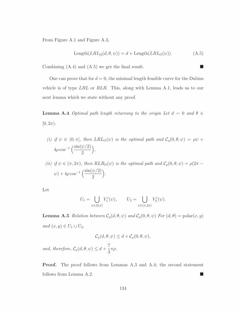
From Figure A.1 and Figure A.3,

Length(LRLO(d, θ, ψ)) = d+ Length(LRLO(ψ)). (A.5)

Combining (A.4) and (A.5) we get the final result.

One can prove that for d = 0, the minimal length feasible curve for the Dubins

vehicle is of type LRL or RLR. This, along with Lemma A.1, leads us to our

next lemma which we state without any proof.

Lemma A.4 Optimal path length returning to the origin Let d = 0 and θ ∈

[0, 2π).

(i) if ψ ∈ (0, π], then LRLO(ψ) is the optimal path and Cρ(0, θ, ψ) = ρψ +

4ρ cos−1(sin(ψ/2)

2

),

(ii) if ψ ∈ (π, 2π), then RLRO(ψ) is the optimal path and Cρ(0, θ, ψ) = ρ(2π −

ψ) + 4ρ cos−1(sin(ψ/2)

2

).

Let

U1 =⋃

ψ∈(0,π]

V c1 (ψ), U2 =

⋃

ψ∈(π,2π)

V c2 (ψ).

Lemma A.5 Relation between Cρ(d, θ, ψ) and Cρ(0, θ, ψ) For (d, θ) = polar(x, y)

and (x, y) ∈ U1 ∪ U2,

Cρ(d, θ, ψ) ≤ d+ Cρ(0, θ, ψ),

and, therefore, Cρ(d, θ, ψ) ≤ d+7

3πρ.

Proof. The proof follows from Lemmas A.3 and A.4; the second statement

follows from Lemma A.2.

134

It now remains to obtain a bound on Cr(d, θ, ψ) when (x, y) ∈ V1(ψ) or

(x, y) ∈ V2(ψ) where (d, θ) = polar(x, y). To this effect, let the vehicle start

moving at time t = 0 at unit speed along Cp1 in the counterclockwise direction

and keep updating the parameters d, θ, ψ as if the coordinate system was moving

along with the vehicle. Consequently V1(ψ) keeps shrinking and there is a time

instant t = t∗ when the final configuration is such that (x, y) /∈ V1(ψ). The

following lemma and its proof contain the details of this constructions and its

implications.

Lemma A.6 For ψ ∈ (0, π), (x, y) ∈ V1(ψ), (d, θ) = polar(x, y) and r > 0,

Cρ(d, θ, ψ) ≤ d+ ρF1(ψ).

Proof. Let Ω0 be a fixed coordinate frame. We define a moving coordinate frame

Ω(t), t ∈ R+, where Ω(0) = Ω0. The origin of Ω(t), denoted as OΩ(t) is defined by

OΩ(t) := [(ρ sin t, ρ− ρ cos t)]Ω0 , where we use the notation [a]B to mean that the

quantity a is to be interpreted in the B frame of reference. Along similar lines

we define the unit vectors along the X and Y direction as:

xΩ(t) = [x cos t+ y sin t]Ω0 , yΩ(t) = [−x sin t+ y cos t]Ω0 ,

where x and y are the unit vectors along the X and Y directions respectively

in Ω0. We introduce the additional notations to interpret the quantities (d, θ) =

polar(x, y) and ψ in different frames of reference.

x = x0 = [x]Ω0 , x(t) = [x]Ω(t), y = y0 = [y]Ω0 , y(t) = [y]Ω(t),

d = d0 = [d]Ω0 , d(t) = [d]Ω(t), θ = θ0 = [θ]Ω0 , θ(t) = [θ]Ω(t),

ψ = ψ0 = [ψ]Ω0 , ψ(t) = [ψ]Ω(t).

135

Also, with a slight abuse of notations, let

V1(ψ)0 = [V1(ψ0)]Ω0 , V1(ψ)(t) = [V1(ψ(t))]Ω(t),

V2(ψ)0 = [V1(ψ0)]Ω0 , V2(ψ)(t) = [V2(ψ(t))]Ω(t).

Let t∗ be the first instant such that (x(t∗), y(t∗)) /∈ V1(ψ)(t∗). Note that t∗ is

a function of θ0 and ψ0, but we drop the arguments for convenience. From the

definition it follows that

ψ(t) = ψ0 − t, θ(t) = θ0 − t. (A.6)

Therefore,

θ(t∗) =ψ(t∗)

2− π

2+ cos−1

(sin(ψ(t∗)/2)

2

). (A.7)

Solving equations (A.6) and (A.7), we get

tan(t∗

2

)=

sin(ψ0/2) − 2 sin(ψ0/2 − θ0)

cos(ψ0/2) + 2 cos(ψ0/2 − θ0).

Now ψ0 ∈ (0, π) implies that θ(t∗) > 0 and t∗ ∈ (0, π), and in turn that t∗ =

F0(ψ0, θ0), where F0 is as defined before Theorem 2.4. Since (x(t∗), y(t∗)) /∈

V1(ψ)(t∗), for ψ0 ∈ (0, π), it follows from Lemmas A.4 and A.5 that

Cρ(d(t∗), θ(t∗), ψ(t∗)) ≤ d(t∗) + ρψ(t∗) + 4ρ cos−1(sin(ψ(t∗)/2)

2

).

Also, it follows from the construction that Cρ(d, θ, ψ) = Cρ(d0, θ0, ψ0) ≤ ρt∗ +

Cρ(d(t∗), θ(t∗), ψ(t∗)). The triangle inequality implies d(t∗) ≤ d0 + 2ρ sin(t∗/2).

From these last equations and equations (A.6), we have

Cρ(d, θ, ψ) = Cρ(d0, θ0, ψ0) ≤ d0 +ρψ0 +2ρ sin(t∗

2

)+4ρ cos−1

(sin((ψ0 − t∗)/2)

2

).

Now, note that, for t∗ = F0(ψ0, θ0) and for α(ψ0) being the half angle of V1(ψ)0,

the supremum of

ψ0 + 2 sin(t∗

2

)+ 4 cos−1

(sin((ψ0 − t∗)/2)

2

)

136

over θ0 ∈ (ψ0

2− α(ψ0),

ψ0

2+ α(ψ0)) is achieved at θ0 = ψ0

2− α(ψ0) and is equal to

F1(ψ0) as defined before Theorem 2.4. Since we are interested in the case when

(x0, y0) ∈ V1(ψ)0, for (d0, θ0) = polar(x0, y0) we have

sup(x0,y0)∈V1(ψ)0

Cρ(d0, θ0, ψ0) ≤ d0 + ρF1(ψ0).

Reverting back to the original notations, i.e., ψ0 = ψ etc., we obtain the desired

result.

From the definition, it follows that for (x, y) 6= (0, 0), (x, y) ∈ V1(ψ) implies

(x, y) ∈ V c2 (ψ). This observation along with part (ii) of Lemma A.3 and part (ii)

of Lemma A.1 leads to the next lemma that we state without proof.

Lemma A.7 For ψ ∈ (0, π], (x, y) ∈ V1(ψ), (d, θ) = polar(x, y) and ρ > 0,

Cρ(d, θ, ψ) ≤ d+ ρF2(ψ).

Lemma A.8 For ψ ∈ (0, π), (x, y) ∈ V1(ψ), (d, θ) = polar(x, y) and ρ > 0,

Cρ(d, θ, ψ) ≤ d+ ρminF1(ψ), F2(ψ).

Therefore, for ψ ∈ (0, π], (x, y) ∈ V1(ψ), (d, θ) = polar(x, y) and ρ > 0,

Cρ(d, θ, ψ) ≤ d+ ρmaxF2(π), supψ∈(0,π)

minF1(ψ), F2(ψ) = d+ κπρ.

Proof. The first statement follows from Lemma A.6 and Lemma A.7. This

along with the consideration for the case of ψ = π easily leads one to the second

statement.

Similarly, one can prove that for ψ ∈ (π, 2π), (x, y) ∈ V2(ψ), (d, θ) =

polar(x, y) and ρ > 0, Cρ(d, θ, ψ) ≤ d+κρ. Combining this with Lemma A.5 and

137

the last statement of Lemma A.8, we can state that for ψ ∈ (0, 2π), (x, y) ∈ R2,

(d, θ) = polar(x, y) and ρ > 0

Cρ(d, θ, ψ) ≤ d+ κr. (A.8)

It now remains to prove a similar bound on Cρ(d, θ, 0) for which we state the

following lemma.

Lemma A.9 For (x, y) ∈ R2, (d, θ) = polar(x, y) and ρ > 0,

Cρ(d, θ, 0) ≤ d+ 2πρ.

Proof. We recall the setup used for the proof of Lemma A.6. In accordance with

that setup,

Cρ(d0, θ0, 0) ≤ d0 + 2ρ sin(t

2

)+ 4ρ cos−1

(sin(−t/2)

2

),

where t > 0. The result follows by taking the limit as t → 0+ and reverting

back to the original notations.

Lemma A.9 combined with equation (A.8) gives the proof for Theorem 2.4. It

is easy to check that for ψ ∈ (0, π), F1(ψ) is a monotonically increasing function

of ψ and F2(ψ) is a monotonically decreasing function of ψ. Therefore, there

exists a unique ψ∗ such that F1(ψ∗) = F2(ψ

∗). By numerical calculations one can

find that κ ≃ 2.6575.

A.3 Numerical Results

The length of the optimal Dubins path, Cρ(d, θ, ψ), was calculated for numer-

ous sets of final configurations (d, θ, ψ) starting with an initial configuration of

138

(0, 0, 0) and a corresponding parameter k was evaluated for each of the instances

according to the relation: Cρ(d, θ, ψ) = d + kπρ. The results suggest that the

value of k is bounded by a quantity, say κnum whose value is equal to 73. More-

over, it appears that k achieves the value of κnum only when the Dubins vehicle

makes a transition from a state of the form (0, 0, 0) to a state of the form (0, 0, π)

according to our setup. Hence, though we do not have an analytical proof to

establish these empirical results exactly, our analysis gives a fairly good estimate

of κnum.

139

Appendix B

Projected Jacobi method

We briefly review here a parallel algorithm for the solution of a quadratic

optimization problem. The technique is known as the projected Jacobi method in

the literature on network flow control problems ([52], Section 3.4).

Consider the quadratic programming problem

minimize1

2xTQx− bTx,

subj. to Ax c,

where Q is a given n× n symmetric positive definite matrix, A is a given m× n

matrix, and b ∈ Rn and c ∈ R

m are given vectors. The dual problem is

minimize1

2yTFy + sTy,

subj. to y 0,

for F = AQ−1AT and s = c − AQ−1b. If y∗ solves the dual problem, then

x∗ = Q−1(b− ATy∗) solves the primal problem.

For a step size parameter τ > 0 and for j ∈ 1, . . . , n, the projected Jacobi

140

iteration, when the jth coordinate is updated, has the form

yj(t+ 1) = max

0, yj(t) −τ

fjj

(sj +

m∑

k=1

fjkyk(t)), (B.1)

where fjk is the j, kth element of the matrix F . As discussed in [52], this algorithm

converges to the global solution of the dual problem if the step size τ is chosen

sufficiently small; in particular, convergence is guaranteed for τ = 1/m.

141

Appendix C

On the Shostak’s test

This section provides a proof for Theorem 6.12. The proof amounts to show-

ing that if E is the edge set of a spanning tree T in Gdi-disk(rcmm, ν(k)rctr) at

(pi, vi)i∈1,...,n, then the control constraint set UdE(rcmm, rctr, ν(k))·(pi, vii∈1,...,n)

is non-empty. We first consider a polytopic approximation of constraints (6.10)

and (6.11). Among all possible choices, we use the conservative orthotope ap-

proximation that allows us to decouple the constraints into d independent sets

of linear inequalities (one for each dimension). Then we use Shostak’s theory

to obtain sufficient conditions for the feasibility of these linear inequalities. For

brevity, we drop the dependence of the quantities on t and we assume that the

variables ui are scalars, for all i ∈ 1, . . . , n and t ≥ 0. The resulting sets of

linear inequalities for one particular dimension are

δli,j ≤ ui − uj ≤ δui,j, and − rctr√d≤ ui ≤

rctr√d. (C.1)

where −ν(k)rctr ≤ δli,j ≤ δui,j ≤ ν(k)rctr, for all i, j ∈ 1, . . . , n and i 6= j.

142

C.1 Shostak Theory

In this section we present Shostak’s theory for feasibility of linear inequalities

involving at most two variables, similar to the ones in (C.1). These ideas will then

be used to prove Theorem 6.12. The notations used in [50] adapted to our case

are presented next. Let u0 be an auxiliary zero variable that always occurs with

zero coefficient - the only variable that can do this. Without loss of generality,

we can thus assume that all the inequalities in L contain two variables. As a

result of this, the inequalities in (C.1) can be succinctly written as

ui − uj ≤ δi,j, ∀i, j ∈ 0, . . . , n, (C.2)

where for all i, j ∈ 1, . . . , n, i 6= j,−ν(k)rctr ≤ δi,j ≤ ν(k)rctr and for all

i ∈ 1, . . . , n, δi,0 = δ0,i = rctr√d. Also implicit in this formulation is the relation

that δi,j + δj,i ≥ 0 for all i, j ∈ 0, . . . , n and i 6= j.

Let L denote the system of inequalities in (C.2). We construct the graph

G(L) with n + 1 vertices and 2(2n − 1) edges as follows: (a) For each variable

ui occurring in L, add a vertex i to G(L). (b) For each inequality of the form

ai,jui + bi,juj ≤ δi,j in L, add an undirected edge between i and j to G(L), and

label the edge with the inequality (see Figure C.1). It is easy to see the following

relation between the spanning tree T in Gdi-disk(rcmm, ν(k)rctr) at (pi, vi)i∈1,...,nthat is used to derive the constraints in the inequalities (C.2) and the graph G(L):

(a) The vertex set of G(L) is the union of the vertex set of T and the auxiliary

vertex 0 (b) For every edge i, j in T , there are two edges between the vertices

i and j in G(L) (c) Additionally, G(L) contains two edges between 0 and every

other vertex i, for all i ∈ 1, . . . , n.

To every edge represented by the inequality of the form ai,jui + bi,juj ≤

143

ui − uj ≤ δi,j

uj − ui ≤ δj,i−ui ≤ rctr√d

−uj ≤ rctr√d

uj ≤ rctr√d

ui ≤ rctr√d

0i

j

Figure C.1: Snippet of the graph G(L) for the system of inequalities in (C.2)

δi,j, we associate a triple 〈ai,j, bi,j, δi,j〉. Note that 〈bi,j, ai,j, δi,j〉 is also a triple

associated with the same edge. Without loss of generality, consider a path of

G(L) determined by the vertices 1, 2, . . . , l+1 and the edges e1,2, e2,3, . . . , el,l+1

between them. A triple sequence, P , associated with the path is defined as

〈a1,2, b1,2, δ1,2〉, 〈a2,3, b2,3, δ2,3〉, . . . , 〈al,l+1, bl,l+1, δl,l+1〉,

where, for 1 ≤ i ≤ l, ai,i+1ui + bi,i+1uj ≤ δi,i+1 is the inequality associated with

the edge ei,i+1. If ai+1,i+2 and bi,i+1 have opposite signs for 1 ≤ i < l, then P is

called admissible.

Define 〈aP , bP , δP 〉, the residue of P , as

〈aP , bP , δP 〉 = 〈a1,2, b1,2, δ1,2〉 ⊙ 〈a2,3, b2,3, δ2,3〉 ⊙ . . .⊙ 〈al,l+1, bl,l+1, δl,l+1〉,

where ⊙ is the associativity binary operator defined on triples by

〈a, b, δ〉 ⊙ 〈a′, b′, δ′〉 = 〈κaa′,−κbb′, κ(δa′ − δ′b)〉,

where κ = a′/|a′|.

Intuitively, the operator ⊙ takes two inequalities and derives a new inequality

by eliminating a common variable; e.g., ax + by ≤ δ and a′y + b′z ≤ δ′ imply

144

−aa′x + bb′z ≤ −(δa′ − δ′b) if a < 0 and b > 0. Note that the signs of aP and

a1,2 agree, as do the signs of bP and b1,2.

A path is called a loop if the initial and final vertices are identical. (A loop

is not uniquely specified unless its initial vertex is given.) If all the intermediate

vertices of a path are distinct, the path is simple. An admissible triple sequence

P associated with a loop with initial vertex x is infeasible if its residue satisfies

aP + bP = 0 and δP < 0. A loop which contains an infeasible triple sequence

is called an infeasible loop. Thus if G(L) has an infeasible loop, the system

of inequalities L is unsatisfiable. However, the converse is not true in general.

Next, we show how to extend L to an equivalent system L′ such that G(L′) has

an infeasible simple loop if and only if L is unsatisfiable.

For each vertex i of G(L) and for each admissible triple sequence P with

aP + bP 6= 0 associated with a simple loop of G(L) and initial vertex i, add a

new inequality (aP + bP )ui ≤ δP to L. This new system L′ is referred to as the

Shostak extension of L. We now state the necessary and sufficient condition on

the extended system of inequalities L′ for the satisfiability of the original system

L.

Theorem C.1 (Shostak’s Theorem [50]) Let L′ be the Shostak extension of

L. The system of inequalities L is satisfiable if and only if G(L′) contains no

infeasible simple loop.

145

C.2 Satisfiability test

In this section we use the Shostak criterion to derive conditions for the satis-

fiability of the inequalities in (C.2).

Lemma C.2 Let L be the system of inequalities of the form (C.2) obtained by

considering pairwise neighbors in a spanning tree T in Gdi-disk(rcmm, ν(k)rctr) at

(pi, vi)i∈1,...,n. Then the Shostak extension of L is itself.

Proof. Consider a simple loop of G(L) with the initial vertex i ∈ 0, 1, . . . , n.

Consider an admissible triple sequence P associated with the loop. Since ai,j, bi,j ∈

−1,+1, for all i, j ∈ 1, . . . , n, i 6= j, and a0,i, ai,0, bi,0, b0,i ∈ −1, 0,+1, for

all i ∈ 1, . . . , n, the residue of P , 〈aP , bP , δP 〉, is such that ap + bp = 0. Hence,

no new inequality must be added to obtain the Shostak extension of L.

Lemma C.3 Let L be the system of inequalities of the form (C.2) obtained

by considering pairwise neighbors in a spanning tree T of depth at most k in

Gdi-disk(rcmm, ν(k)rctr) at (pi, vi)i∈1,...,n. If ν(k) = 2k√d, then there is no infea-

sible simple loop in G(L).

Proof. Looking at figure C.1 it is clear that there are two types of simple loops

with admissible triple sequences in G(L):

(i) 〈+1,−1, δi,j〉, 〈+1,−1, δj,i〉 or 〈−1,+1, δi,j〉, 〈−1,+1, δj,i〉,

where i, j ∈ 0, . . . , n− 1 and i, j is an edge in T .

146

(ii) 〈0,−1, rctr√d〉, 〈+1,−1, δi1,i2〉, . . . , 〈+1,−1, δil−1,il〉, 〈+1, 0, rctr√

d〉 or

〈0,+1, rctr√d〉, 〈−1,+1, δi2,i1〉, . . . , 〈−1,+1, δil,il,l−1

〉, 〈−1, 0, rctr√d〉,

where il ∈ 1, . . . , ζ for all l ∈ 1, . . . , ζ and il, il+1 is an edge in T .

The residue for the first set of loops is 〈+1,−1, δi,j + δj,i〉 or 〈−1,+1, δi,j + δj,i〉.

The feasibility condition is trivially satisfied by construction since δi,j + δj,i ≥ 0.

For the second set of loops, the residue is:

⟨0,−1,

rctr√d

⟩⊙ 〈+1,−1, δi1,i2〉 ⊙ . . .⊙ 〈+1,−1, δiζ−1,iζ〉 ⊙

⟨+ 1, 0,

rctr√d

⟩

=⟨0, 0, 2

rctr√d

+

ζ−1∑

l=1

δil,il+1

⟩,

or

⟨0,+1,

rctr√d

⟩⊙ 〈−1,+1, δi2,i1〉 ⊙ . . .⊙ 〈−1,+1, δiζ ,iζ−1

〉 ⊙⟨− 1, 0,

rctr√d

⟩

=⟨0, 0, 2

rctr√d

+

ζ−1∑

l=1

δil,il+1

⟩.

In order to guarantee the feasibility of the second set of loops, we need that

2 rctr√d

+∑ζ−1

l=1 δil,il+1≥ 0. We derive conditions for the worst case which occurs

when the loop is written for the longest path in T , i.e., when ζ = k+1 and when

δil,il+1= −ν(k)rctr, for all l ∈ 1, . . . , k. In this case, there is no infeasible simple

loop if and only if

2rctr√d− kν(k)rctr ≥ 0,

that is, if and only if ν(k) = 2k√d.

Finally, the proof of Theorem 6.12 follows from Theorem C.1, Lemma C.2

and Lemma C.3.

147