university of california...curriculum vit‰ ankur saxena education 2008 ph.d. in electrical and...

UNIVERSITY of CALIFORNIA

Santa Barbara

Distributed coding of spatio-temporally correlated sources

A Dissertation submitted in partial satisfaction of the

requirements for the degree

Doctor of Philosophy

in

Electrical and Computer Engineering

by

Ankur Saxena

Committee in charge:

Professor Kenneth Rose, Chair

Professor Jerry Gibson

Professor Upamanyu Madhow

Professor B. S. Manjunath

Professor Tor A. Ramstad

December 2008

3342044

3342044 2009

The dissertation of Ankur Saxena is approved.

Professor Jerry Gibson

Professor Upamanyu Madhow

Professor B. S. Manjunath

Professor Tor A. Ramstad

Professor Kenneth Rose, Committee Chair

November 2008


Copyright c© 2008

by

Ankur Saxena

iii

To my brother and my parents.

iv

Acknowledgements

First of all I would like to express my gratitude towards my advisor Prof

Kenneth Rose for his encouragement, patience and support during my graduate

studies. I am grateful to him for the right mix of guidance and freedom that I

received and have benefitted immensely from his sharp insight and ability to see

the bigger picture.

I would like to thank Prof Upamanyu Madhow and Prof Shiv Chandrasekaran

for teaching wonderful classes in communication theory and linear algebra. I am

also grateful to Prof Jerry Gibson, Prof B. S. Manjunath and Prof Tor Ramstad

for being on my doctoral committee.

The research presented here was supported by the National Science Founda-

tion (IIS-0329267 and CCF-0728986), and in part by the University of California

MICRO program, Applied Signal Technology Inc., Cisco Systems Inc., Dolby

Laboratories Inc., Qualcomm Inc., and Sony Ericsson, Inc.

A big thanks to Jayanth Nayak for his help and valuable advice in the early

research days. Thanks to Sumit Paliwal and Kaviyesh Doshi for encouraging me

throughout my graduate student life.

Thanks to Sharadh Ramaswamy for being a great friend and lab-mate in the

Signal Compression Lab. I would also like to thank Christan Schmidt, Jaspreet

Singh and Vinay Melkote for the numerous stimulating discussions in the lab and

during lunch time. Working in SCL was always enjoyable due to the presence of

wonderful lab-mates: Hua, Sang, Alphan, Pakpoom, Jaewoo, Emre and Emrah.

I am thankful to the ECE support staff, especially Valerie de Veyra for the

v

much needed help in administrative work.

I would always cherish the great company of my friends Gaurav Soni and

Amitabh Virmani who were my family away from home in Santa Barbara. They

were always there to listen and help me in my endeavors. Special thanks to

Anshuman Maharana for lots of delicacies in this part of the world. For the great

fun and activities, I would also thank Anindya Sarkar, Raj Sau, Pratim Ghosh,

Anand Meka and Vineet Wason.

I thank my family for all the support and motivation throughout my studies,

particulary my younger brother Mohit, and most importantly my parents for

everything they have done for me.

vi

Curriculum Vitæ

Ankur Saxena

Education

2008 Ph.D. in Electrical and Computer Engineering, University ofCalifornia, Santa Barbara.

2004 Master of Science in Electrical and Computer Engineering, Uni-versity of California, Santa Barbara.

2003 B.Tech in Electrical Engineering, Indian Institute of Technology-Delhi.

Research Experience

2004 – 2008 Graduate Research Assistant, University of California, SantaBarbara.

Summer 2007 Student Research Intern, NTT Docomo Labs, Palo Alto, CA.Summer 2002 Student Intern, Fraunhofer Institute of X-Ray Technology, Er-

langen, Germany.

Publications

1. Distributed predictive coding for spatio-temporally correlated sourcesAnkur Saxena and Kenneth Rose, under review in IEEE Transactions on SignalProcessing.

2. Optimized system design for robust distributed source codingAnkur Saxena, Jayanth Nayak and Kenneth Rose, under review in IEEE Trans-actions on Signal Processing.

3. On scalable coding of correlated sourcesAnkur Saxena and Kenneth Rose, to be submitted to IEEE Transactions on SignalProcessing.

4. Scalable distributed source codingAnkur Saxena and Kenneth Rose (submitted to IEEE International Conferenceon Acoustics, Speech, and Signal Processing, 2009).

5. Optimization of correlated source coding for event-based compression in sensornetworksJaspreet Singh, Ankur Saxena, Kenneth Rose and Upamanyu Madhow (submittedto IEEE Data Compression Conference, 2009).

vii

6. On distributed quantization in scalable and predictive codingAnkur Saxena and Kenneth Rose (Proc. Sensor, Signal and Information Process-ing, May 2008).

7. Distributed multi-stage coding of correlated sourcesAnkur Saxena and Kenneth Rose (IEEE Data Compression Conference, March2008).

8. Challenges and recent advances in distributed predictive codingAnkur Saxena and Kenneth Rose (Invited Paper) (IEEE Information TheoryWorkshop, Sept 2007).

9. Distributed predictive coding for spatio-temporally correlated sourcesAnkur Saxena and Kenneth Rose (IEEE International Symposium on InformationTheory, June 2007).

10. A global approach to joint quantizer design for distributed coding of correlatedsourcesAnkur Saxena, Jayanth Nayak and Kenneth Rose (IEEE International Conferenceon Acoustics, Speech, and Signal Processing, May 2006).

11. On efficient quantizer design for robust distributed source codingAnkur Saxena, Jayanth Nayak and Kenneth Rose (IEEE Data Compression Con-ference, March 2006).

viii

Abstract


by

Ankur Saxena

This dissertation studies certain problems in distributed coding of correlated

sources. The first problem considers the design of efficient coders in a robust dis-

tributed source coding scenario. Here, the information is encoded at independent

terminals and transmitted across separate channels, any of which may fail. This

scenario subsumes a wide range of source and source-channel coding/quantization

problems, including multiple descriptions and the CEO problem. A global op-

timization algorithm based on deterministic annealing is proposed for the joint

design of all the system components. The proposed approach avoids many poor

local optima, is independent of initialization, and does not make any simplifying

assumption on the underlying source distribution.

The second problem considered is of scalable distributed source coding. This

is the general setting typically encountered in sensor networks. The conditions

of channels between the sensors and the fusion center may be time-varying and

it is often desirable to guarantee a base layer of coarse information during chan-

nel fades. This problem poses new challenges. Multi-stage distributed coding, a

special case of scalable distributed coding, is considered first. The fundamental

conflicts between the objectives of multi-stage coding and distributed quanti-

ix

zation are identified and an appropriate design strategy is devised to explicitly

control the tradeoffs. The unconstrained scalable distributed coding problem

is considered next. Although standard greedy coder design algorithms can be

generalized to scalable distributed coding, the resulting algorithms depend heav-

ily on initialization. An efficient initialization scheme is devised which employs

a properly designed multi-stage distributed coder. The proposed design tech-

niques for multi-stage and unconstrained scalable distributed coding scenarios

offer substantial gains over naive approaches for multi-stage distributed coding

and randomly initialized scalable distributed coding respectively.

The third problem considered is distributed coding of sources with memory.

This problem poses a number of considerable challenges that threaten the prac-

tical application of distributed coding. Most common sources exhibit temporal

correlations that are as important as inter-source correlations. Motivated by

practical limitations on both complexity and delay, especially for dense sensor

networks, the problem is re-formulated in its fundamental setting of distributed

predictive coding. The most basic tradeoff (and difficulty) is due to the con-

flicts that arise between distributed coding and prediction, wherein ‘standard’

distributed quantization of the prediction errors, if coupled with imposition of

zero decoder drift, drastically compromises the predictor performance and hence

the ability to exploit temporal correlations. Another challenge arises from in-

stabilities in the design of closed loop predictors in distributed coding setting.

These fundamental tradeoffs in distributed predictive coding are identified and a

more general paradigm, is proposed where decoder drift is allowed but explicitly

controlled. The proposed paradigm avoids the pitfalls of naive techniques and

produces an optimized low complexity and low delay coding system.

x

Contents

Acknowledgements v

Curriculum Vitae vii

Abstract ix

List of Figures xiv

List of Acronyms xvii

1 Introduction 1

1.1 Globally optimal algorithms for distributed source coding . . . . . 3

1.2 Scalable distributed source coding . . . . . . . . . . . . . . . . . . 5

1.3 Distributed coding of correlated sources with memory . . . . . . . 6

2 Preliminaries and Background 9

2.1 Vector quantizer . . . . . . . . . . . . . . . . . . . . . . . . . . . . 9

2.1.1 Necessary conditions for optimality . . . . . . . . . . . . . 11

2.1.2 The generalized Lloyd design algorithm . . . . . . . . . . . 13

2.2 Distributed source coding . . . . . . . . . . . . . . . . . . . . . . 14

2.2.1 Background . . . . . . . . . . . . . . . . . . . . . . . . . . 14

2.2.2 Distributed source coder . . . . . . . . . . . . . . . . . . . 16

2.3 Summary . . . . . . . . . . . . . . . . . . . . . . . . . . . . . . . 17

xi

3 Global optimization for distributed source coding 18

3.1 Robust distributed source coding . . . . . . . . . . . . . . . . . . 19

3.1.1 Design challenges and the need for global optimization tech-niques . . . . . . . . . . . . . . . . . . . . . . . . . . . . . 19

3.2 The RDVQ problem and iterative greedy methods . . . . . . . . 21

3.2.1 Problem statement and design considerations . . . . . . . 21

3.2.2 Greedy iterative design strategy . . . . . . . . . . . . . . . 24

3.3 The deterministic annealing approach . . . . . . . . . . . . . . . . 26

3.3.1 Derivation for RDVQ setup . . . . . . . . . . . . . . . . . 27

3.3.2 Update Equations for RDVQ Design . . . . . . . . . . . . 30

3.4 Simulation results . . . . . . . . . . . . . . . . . . . . . . . . . . . 33

3.5 Conclusions . . . . . . . . . . . . . . . . . . . . . . . . . . . . . . 40

4 Scalable coding of correlated sources 41

4.1 Problem statement and special cases . . . . . . . . . . . . . . . . 43

4.1.1 Special Cases . . . . . . . . . . . . . . . . . . . . . . . . . 45

4.2 Multi-stage distributed source coding . . . . . . . . . . . . . . . . 47

4.2.1 Encoder . . . . . . . . . . . . . . . . . . . . . . . . . . . . 47

4.2.2 Decoder . . . . . . . . . . . . . . . . . . . . . . . . . . . . 49

4.2.3 Components to optimize . . . . . . . . . . . . . . . . . . . 50

4.2.4 Naive design scheme . . . . . . . . . . . . . . . . . . . . . 50

4.2.5 Comments on naive design scheme . . . . . . . . . . . . . 51

4.3 Multi-stage distributed coding design algorithm . . . . . . . . . . 52

4.3.1 Motivation and design . . . . . . . . . . . . . . . . . . . . 52

4.3.2 Update rules for proposed MS-DSC algorithm . . . . . . . 54


4.4.1 Iterative design algorithm . . . . . . . . . . . . . . . . . . 58

4.4.2 Effective initialization for S-DSC design . . . . . . . . . . 59


4.6 Conclusions . . . . . . . . . . . . . . . . . . . . . . . . . . . . . . 66

xii

5 Distributed predictive coding 68

5.1 Predictive vector quantizer design for single-source . . . . . . . . 70

5.1.1 Open loop approach . . . . . . . . . . . . . . . . . . . . . 71

5.1.2 Closed loop approach . . . . . . . . . . . . . . . . . . . . . 72

5.1.3 The asymptotic closed loop approach . . . . . . . . . . . . 74

5.2 DPC:Problem statement . . . . . . . . . . . . . . . . . . . . . . . 76

5.3 Zero-drift approach . . . . . . . . . . . . . . . . . . . . . . . . . . 78

5.3.1 Encoder . . . . . . . . . . . . . . . . . . . . . . . . . . . . 78

5.3.2 Decoder . . . . . . . . . . . . . . . . . . . . . . . . . . . . 79

5.3.3 Observations and intuitive considerations . . . . . . . . . . 80

5.3.4 Naive approach for DPC design . . . . . . . . . . . . . . . 80

5.3.5 Closed loop vs ACL design . . . . . . . . . . . . . . . . . . 82

5.4 ACL for zero-drift distributed predictive coding . . . . . . . . . . 83

5.4.1 Update rules: zero-drift DPC . . . . . . . . . . . . . . . . 84

5.4.2 Predictor optimization . . . . . . . . . . . . . . . . . . . . 85

5.4.3 Algorithm description . . . . . . . . . . . . . . . . . . . . 87

5.5 Controlled-drift approach . . . . . . . . . . . . . . . . . . . . . . . 89

5.5.1 Motivation and description . . . . . . . . . . . . . . . . . . 89

5.5.2 Controlled-drift DPC-Update rules . . . . . . . . . . . . . 91


5.6.1 Convergence of DPC:ACL algorithms . . . . . . . . . . . . 95

5.7 Conclusions . . . . . . . . . . . . . . . . . . . . . . . . . . . . . . 97

6 Conclusions and Future Directions 98

6.1 Main contributions . . . . . . . . . . . . . . . . . . . . . . . . . . 99

6.2 Future directions . . . . . . . . . . . . . . . . . . . . . . . . . . . 101

A Critical temperature derivation for phase transition in annealing102

Bibliography 108

xiii

List of Figures

1.1 A sensor network scenario, where different sensors are transmittinginformation to a fusion center . . . . . . . . . . . . . . . . . . . . 3

2.1 Schematic of a vector quantizer . . . . . . . . . . . . . . . . . . . 10

2.2 Voronoi regions induced by a 2-d VQ for squared error distortionmeasure. . . . . . . . . . . . . . . . . . . . . . . . . . . . . . . . . 12

2.3 Distributed coding of two correlated sources . . . . . . . . . . . . 17

3.1 Block diagram for robust distributed source coding . . . . . . . . 19

3.2 Breakup of encoder in robust distributed source coding . . . . . . 21

3.3 An example of Wyner-Ziv mapping from prototypes (Voronoi re-gions) to indices. . . . . . . . . . . . . . . . . . . . . . . . . . . . 24

3.4 Comparison between LA and DA approaches for R1 = 3 , R2 = 4,K = 64, L = 128, α0 = 0.5, α1 = 1, α2 = 0, λ0 =1, λ1 = λ2 =0.01. Net distortion from DA is -16.98 dB while LA gives best andworst distortion as -15.69 and -12.77 dB, respectively. For ease ofcomparison, a line along which constant Dnet = -16.98 dB is drawn. 35

3.5 Comparison between LA and DA approaches for R1 = 2, R2 = 3,K = L = 64, α0=α1=α2= 0.5, λ0 =1, λ1 = 0.005 , λ2 = 0.01. Netdistortion from DA is -13.44 dB while LA gives best and worstdistortion as -12.18 and -10.54 dB, respectively. For ease of com-parison, a line along which constant Dnet = -13.44 dB is drawn. . 36

xiv

3.6 Comparison between LA and DA approaches for a distributed vec-tor quantizer of dimension 2. R1 = R2 = 2, K = L = 128, α0 =0.5, λ0 =1, λ1 = λ2 = 0. Net distortion from DA is -12.75 dBwhile LA gives best and worst distortion as -10.85 and -10.01 dB,respectively. For ease of comparison, a line along which constantDnet = -12.75 dB is drawn. Achievable distortion as promised in[54] is -15.61 dB. . . . . . . . . . . . . . . . . . . . . . . . . . . . 37

3.7 Comparison between LA and DA approaches for a distributed vec-tor quantizer for sources coming from a gaussian mixture model.R1 = R2 = 3 , K = L = 64, α0 = 0.5, λ0 =1, λ1 = λ2 = 0. Netdistortion from DA is -13.59 dB while LA gives best and worstdistortion as -12.74 and -9.87 dB, respectively. For ease of com-parison, a line along which constant Dnet = -13.59 dB is drawn. . 38

3.8 Comparison between LA and DA approaches when the number ofsource prototypes are varied for R1 = R2 = 3 α0 = α1 = α2 = 0.5;λ0 =1, λ1 = λ2 = 0.01. . . . . . . . . . . . . . . . . . . . . . . . 39


4.2 MS-DSC encoder and an example of Wyner-Ziv mapping fromVoronoi regions to (transmitted) indices . . . . . . . . . . . . . . 48

4.3 MS-DSC decoders D00 and D10 for source X . . . . . . . . . . . . 49

4.4 S-DSC encoder for source X; an example of Wyner-Ziv mappingfrom Voronoi regions to index pair {i1, i2}; and decoders D00 andD10 in S-DSC . . . . . . . . . . . . . . . . . . . . . . . . . . . . . 57

4.5 Performance comparison of naive scheme for MS-DSC, separate(single source) multi-stage coding, randomly initialized scalableDSC, proposed multi-stage DSC, and proposed scalable DSC tech-nique. (a) All the transmission rates are same and varied; (b)enhancement layer rates are varied (base layer rates fixed at 2bits/sample); (c) base layer rates are varied (enhancement layerrates fixed at 2 bits/sample). . . . . . . . . . . . . . . . . . . . . . 62

4.6 Performance comparison of separate (single source) multi-stagecoding, randomly initialized scalable DSC, proposed multi-stageDSC, and proposed scalable DSC technique as the probability ofenhancement layer loss px(= py) is varied. All the transmissionrates are 2 bits/sample. In (a) inter-source correlation ρ = 0.97while in (b) ρ = 0.9. . . . . . . . . . . . . . . . . . . . . . . . . . 63

xv

4.7 Performance comparison of separate (single source) multi-stagecoding, randomly initialized scalable DSC, proposed multi-stageDSC, and proposed scalable DSC technique as the inter-sourcecorrelation is varied. All the transmission rates are 2 bits/sample.The probability of enhancement layer loss px(= py) is 0.2 in (a)and 0.1 in (b). . . . . . . . . . . . . . . . . . . . . . . . . . . . . . 64

5.1 Predictive vector quantizer . . . . . . . . . . . . . . . . . . . . . . 72

5.2 Open loop approach for PVQ design . . . . . . . . . . . . . . . . 73

5.3 Closed loop approach . . . . . . . . . . . . . . . . . . . . . . . . . 74

5.4 Asymptotic closed loop approach . . . . . . . . . . . . . . . . . . 76

5.5 Distributed coding of two correlated sources . . . . . . . . . . . . 77

5.6 Block diagram of a DPC zero-drift encoder and a scalar exampleof WZ mapping from prototypes (Voronoi regions) to indices. . . . 79

5.7 DPC zero-drift decoder for source X . . . . . . . . . . . . . . . . 79

5.8 DPC zero-drift decoder in open loop during the design phase . . . 83

5.9 Flowchart of asymptotic closed loop design procedure for distributedpredictive coding . . . . . . . . . . . . . . . . . . . . . . . . . . . 88

5.10 Controlled-drift DPC encoder . . . . . . . . . . . . . . . . . . . . 90

5.11 Controlled-drift DPC decoder . . . . . . . . . . . . . . . . . . . . 90

5.12 Controlled-drift DPC decoder during design phase . . . . . . . . . 90

5.13 Performance comparison of distributed predictive coding schemes,non-distributed predictive coding, and memoryless distributed cod-ing. Figures (a) and (c) show weighted distortion vs. rate andinter-source correlation respectively. Figure (b) shows SNR vs.temporal correlation . . . . . . . . . . . . . . . . . . . . . . . . . 94

5.14 Plot showing the convergence of various distributed predictive cod-ing algorithms. Here ρ = 0.98, β = γ = 0.8, R1 = R2 = 2bits/sample . . . . . . . . . . . . . . . . . . . . . . . . . . . . . . 96

xvi

List of Acronyms

ACL : Asymptotic closed loopbps : bits per source sampleCL : Closed loopDA : Deterministic annealingdB : DecibelDPC : Distributed predictive codingDSC : Distributed source codingGLA : Generalized Lloyd algorithmLA : Lloyd’s approach (adapted to distributed quantizer design)MP : Multiple prototypesMS-DSC : Multi-stage distributed source codingMSE : Mean squared errorOL : Open loopPVQ : Predictive vector quantizerRDVQ : Robust distributed vector quantizerS-DSC : Scalable distributed source codingSNR : Signal to noise ratioVQ : Vector quatizerWZ : Wyner-Ziv

xvii

Chapter 1

Introduction

Shannon’s seminal work in the middle of the previous century [47] started

the field of information theory. The two main sub-fields of information theory

are source coding and channel coding. Source coding primarily deals with com-

pression of signals by exploiting the redundancies within the source sequence.

Channel coding typically involves the use of error correcting codes to protect the

data during transmission over a noisy channel.

In source coding, the compression can either be lossless or lossy. Lossless

compression is used when exact reconstruction of the sources is required such as

in medical imaging, bank transactions, where all the source bits are important.

Lossy compression is used when some distortion in the source reconstruction

can be tolerated. For example, in practical multimedia compression scenarios

involving speech, audio, video and image signals, lossy compression schemes are

employed to reduce rate at the expense of introducing some distortion.

This dissertation considers lossy compression in the context of distributed

1

(multi-terminal) source coding, i.e, when multiple sources are communicated via

different channels to a fusion center. An application of distributed source coding

is in sensor networks, where different sensors may be designed to observe various

physical quantities, e.g., temperature, humidity, pressure, light, sound. We may

be interested in efficient reconstruction of one or more physical entities measured

at different, spatially separated locations. A figure with M sensors S1, S2, ..., SM

transmitting information to a fusion center is shown in Fig. 1.1. Sensors, in a

sensor network often have stringent power and bandwidth constraints that pre-

clude inter-sensor communication. However, the data communicated by networks

of sensors exhibit a high degree of correlation. Hence the design of encoders at

all sensor locations and decoders at the fusion center should be performed jointly

in order to achieve optimality. Further, the sensor (source) data will exhibit

temporal correlations as well, which may be at least as important as inter-source

correlations. A related issue is that of estimation of a source from another, cor-

related source. For example, if a sensor (or a transmission channel) fails, then to

obtain an estimate of data being (or that would be) measured by the sensor, we

can only utilize information acquired from the other sensors (or channels). This

work targets the objectives of (a) efficiently exploiting both the temporal and

inter-source correlation between sources to obtain the best possible compression

efficiency from independent encoders and (b) achieving system robustness for dif-

ferent source and channel conditions within various distributed coding paradigms.

The dissertation is divided into three main parts. In the first part, introduced

in Sec. 1.1, we propose a global design algorithm based on deterministic annealing

for distributed source coding system. The second part introduced in Sec 1.2 is

concerned with scalable distributed source coding. Here we identify the funda-

2

(X1, X2, ..., XM)

...............................

.................................................................................................................................................................................................................................................................................................

.........................

...............................

.................................................................................................................................................................................................................................................................................................

......................... ...............................................................................................................................................................................................................................................................................................

..............................................................

..................

................................................................................

........................................................................................................................................................................................................................................................................................................................................

................................................................................

...............................................................................................

...............

...............

...............

...............

...............

...............

................................................................................

................................................................................

................................................................................

Encoder 1

Encoder 2

Encoder M

S1

S2

SM

JointDecoder

X1

XM

X2...............................

.................................................................................................................................................................................................................................................................................................

.........................

Figure 1.1. A sensor network scenario, where different sensors are transmitting

information to a fusion center

mental conflicts between scalable coding and distributed quantization and devise

strategies for he special case of multi-stage distributed coding, and the general

scalable distributed coding systems. The third part introduced in Sec. 1.3 con-

siders distributed coding of sources with memory. This problem poses numerous

new challenges. We specifically employ predictive coding to exploit the temporal

redundancies and formulate the problem in its fundamental setting of distributed

predictive coding. We identify the fundamental conflicts that arise when dis-

tributed coding is naively combined with predictive coding and devise various

design strategies for the distributed predictive coding scenarios.

1.1 Globally optimal algorithms for distributed

source coding

The data communicated by various sensors (say, monitoring a physical phe-

nomenon such as temperature) in a sensor network typically exhibits a high degree

of correlation. The encoders at each sensor location function independently, but

3

joint design of various system components is necessary to achieve the highest

compression rate. To achieve the dual objectives of obtaining the best possible

compression efficiency from independent encoders and attaining system robust-

ness (in case of source or channel failure), it is necessary that the code design at

all the terminals be performed jointly for such a robust distributed source coding

system.

The robust distributed source coding model subsumes a variety of source cod-

ing problems ranging from distributed source coding [48, 56], the CEO problem

[2], to multiple description coding [29]. Estimating a source from another corre-

lated source (see e.g., [16, 33]) is another special case of the robust distributed

coding problem.

We focus on source coding methodologies to design a robust distributed coding

system. Greedy design approaches, such as those based on the Lloyd’s algorithm

[26] suffer from the presence of numerous ‘poor’ local minima on the distortion-

cost surface and thus will be critically sensitive to initialization. Clever initial-

ization as proposed, for example, in the context of multiple description scalar

quantizer design [53], can help mitigate this shortcoming. But such initialization

heavily depends on symmetries or simplifying assumptions, and no generaliza-

tions are available to vector quantization nor to more complicated scenarios such

as in robust distributed source coding. Alternatively, a powerful optimization

tool such as deterministic annealing (DA) provides the ability to avoid poor local

optima and is applicable to sources exhibiting any type of statistical dependen-

cies. In Chapter 3, we present a locally optimal Lloyd-based algorithm for robust

distributed coding design as well as the DA based scheme for robust distributed

coding design including the necessary rules for optimality.

4

1.2 Scalable distributed source coding

The second problem that we consider is that of scalable distributed coding

of correlated sources. The general setting is typically encountered in sensor net-

works. The conditions of communication channels between the sensors and fusion

center may be time-varying and it is often desirable to guarantee a base layer of

coarse information during channel fades. In addition, the desired system should

be robust to various scenarios of channel failure and should utilize all the available

information to attain the best possible compression efficiency.

Our contribution to the problem is twofold. We begin by considering a multi-

stage distributed coding system, a special constrained case of scalable distributed

coding. This problem poses new challenges. We show that mere extensions of dis-

tributed coding ideas to include multi-stage coding yield poor rate-distortion per-

formance, due to underlying conflicts between the objectives of multi-stage and

distributed quantization. An appropriate system paradigm is developed which

allows such tradeoffs to be explicitly controlled within joint optimization of all

the system components. Next, we consider the unconstrained scalable distributed

coding problem. Although a standard Lloyd-like distributed coder design algo-

rithm can be generalized to scalable distributed coding, the resulting algorithm

depends heavily on initialization and will virtually always converge to a poor

local minimum on the cost surface. In Chapter 4, we propose an efficient initial-

ization scheme for such a system, which employs a properly designed multi-stage

distributed coder. We present iterative joint design techniques and derive the

necessary conditions for optimality for both multi-stage and unconstrained scal-

able distributed coding systems. Simulation results show substantial gains for

5

the proposed multi-stage distributed coding system over single source (separate)

multi-stage coding as well as naive extensions to incorporate scalability in multi-

stage distributed coding system. Further the performance of proposed efficiently

initialized scalable distributed coder is considerably better than randomly initial-

ized scalable distributed coder.

1.3 Distributed coding of correlated sources with

memory

In the third part of the dissertation, we study distributed source coding (DSC)

for sources with memory. In real world applications most sources exhibit tempo-

ral correlations. Examples range from simple sensors monitoring slowly varying

physical quantities such as temperature or pressure, to the extreme of video cam-

eras collecting highly correlated frame sequences.

Realizing the prevalence of sources with memory and the importance of ex-

ploiting both temporal and inter-source correlation, we reformulate the problem

within the representative setting of distributed predictive coding (DPC) systems.

Given the historical focus on inter-source correlations in DSC, most existing DSC

work naturally addressed memoryless sources where one need not worry about

temporal correlations. The implicit assumption may have been that predictive

coding per se is a largely solved problem, and that extending DSC results to

incorporate prediction would require a straightforward integration phase. (An al-

ternative argument may involve handling long blocks of source data, as in vector

quantization to exploit time correlations, but the cost in delay and complexity

6

may be considerable). We show that the generalization from DSC to DPC is

highly non-trivial due to conflicting objectives of distributed coding versus effi-

cient prediction in DPC. In other words, optimal distributed coding (in terms of

current reconstruction quality) may severely compromise the prediction loop at

each source encoder. We have proposed new DPC system paradigms and methods

to optimize their design in Chapter 5.

Another design difficulty whose origins are in traditional single-source predic-

tive quantizer design [17] is exacerbated in the distributed setting. On the one

hand, open loop design is simple and stable but the quantizer is mismatched with

the true prediction error statistics (as the system eventually operates in closed

loop). On the other hand, if a distributed quantizer is designed in closed loop, the

effects of quantizer modifications are unpredictable as quantization errors are fed

back through the prediction loop and can build up. Hence the procedure is unsta-

ble and may not converge. The effect is greatly exacerbated in the case of DPC.

To circumvent these difficulties, we have used the technique of asymptotic closed

loop (ACL) design [19, 20] which we re-derive for DPC system design. Within

the DPC-ACL framework, the design is effectively in open loop within iterations

(eliminating issues of error buildup through the prediction loop), while ensur-

ing that asymptotically, the prediction error statistics converge to closed loop

statistics. In other words, the prediction loop is essentially closed asymptotically.

In Chapter 5, we derive an overall design optimization method for distributed

predictive coding that avoids the pitfalls of naive distributed predictive quanti-

zation and produces an optimized low complexity and low delay coding system.

The proposed iterative algorithms for distributed predictive coding subsume tra-

ditional single-source predictive coding and memoryless distributed coding as

7

extreme special cases.

8

Chapter 2

Preliminaries and Background

In this chapter, we first explain the functioning of a vector quantizer (VQ),

provide background for distributed source coding, and introduce the main build-

ing blocks for the simplest quantization-based distributed source coding system.

2.1 Vector quantizer

In most lossy compression applications, the source is quantized or discretized

to a reduced number of reconstruction values. This operation is performed by

a quantizer (see Fig. 2.1). The earliest design method of a scalar quantizer is

due to Lloyd in an unpublished paper in 1957 (later published as [26] in 1982)

and Max in 1960, [27]. The vector quantizer is a straightforward extension of

the scalar quantizer and the corresponding design method called the Generalized

Lloyd Algorithm (GLA) was presented by Linde, Buzo and Gray in 1980 [24],

although it has earlier roots in both compression and pattern recognition. In

9

X...........................

.....................................................

................................................................................ Decoder DEncoder E Xi

................................................................................

Figure 2.1. Schematic of a vector quantizer

clustering, the k-means algorithm closely resembles the GLA algorithm for VQ

design. In general, the VQ design problem is NP-hard and all the afore mentioned

algorithms try to find a good locally optimal solution. In addition, annealing-

based algorithms inspired from concepts in statistical physics, which try to find

the global optimum have also been proposed for VQ design in [21],[36],[37].

Fig. 2.1 shows the simplest VQ implementation which subsumes the scalar

quantizer as special case. VQ consists of two modules, an encoder and a decoder.

Source signal X is input to a source encoder E . The encoder output is an index

i = E(X) which takes one of the values from the set {1..I}. The decoder module

takes the index i as input and outputs an approximation X = D(i) for the source.

Possible reconstruction values X are called the codevectors, and the set of all

codevectors is called the codebook. It is desired that the source reconstruction

X closely resembles the original source X within a fidelity criterion, given by the

following expected distortion cost:

D =1

nE[d(X, X)] (2.1)

for a given rate of the VQ given by:

R =1

nlog2 I (2.2)

bits per source sample. Here d(·, ·) is an appropriately defined distortion measure

and n is the vector dimension. In most applications, the distortion measure d(·, ·)is assumed to be mean squared error (MSE) primarily because of its analytic

10

simplicity and its interpretation as the energy of the error signal. Numerous

other distortion measures are used in the compression literature, see e.g., [12] in

which various quality measures for gray-scale image compression and the resulting

performance is presented.

VQ is, in fact, a generalization of almost all compression schemes, such as

predictive coding, transform coding etc. For sources with memory, VQ’s perfor-

mance is better than that of scalar quantizers, since VQ can exploit the corre-

lations between source samples. Even for a memoryless i.i.d. source, VQ can

perform better than scalar quantizers since a better covering can be devised for

a higher dimensional space (e.g., hexagonal partition in 2-d space is better than

the rectangular covering induced by scalar quantizer ([17], Chp. 11, Page 347)).

As mentioned above, the objective of the VQ is to minimize the expected

distortion E[d(X, X)] for a given input distribution for source X via efficient

design of the encoder and decoder modules under prescribed rate constraints.

However, the optimal VQ design problem is NP-hard and a closed form solution

is not available. Typical design procedures alternate between encoder and decoder

module design. Next we outline the necessary conditions for optimality of a VQ

system, followed by a sketch of the GLA algorithm for fixed-rate VQ design.

2.1.1 Necessary conditions for optimality

The necessary condition for optimal encoding is: a data point x gets mapped

to index i and is reconstructed by xi if

d(x, xi) ≤ d(x, xj) ∀i 6= j (2.3)

11

1

w

w

w

w

w

.................................................................................................................................................................................................................................

........

........

........

........

........

........

........

........

........

........

........

........

........

........

........

........

........

........

........

........

........

........

........

........

........

........

........

........

........

........

........

........................................................................................................................................................................................................................................................................................................................................................................

........................................................................................................................................................................

........................................................................................................................................................................

.....................................................................................................................................................................................................................................................................................................................

........................................................................................................................................................................................................................................................................................................................................

...................................................................................................................................................................................................................................................................................................................................................................................................................................................................................................................................................................................................................................................................................................................................................................................

6

5

4

3

2

w

Figure 2.2. Voronoi regions induced by a 2-d VQ for squared error distortion

measure.

The points x which map to index i will form a region Ri = {x : d(x, xi) ≤d(x, xj)}. The regions Ri are disjoint and cover the entire source space, i.e., if X

is a n-dimension vector in Rn, then:

⋃i

Ri = Rn and Ri

⋂Rj = φ ∀{i, j ∈ {1..I}, i 6= j} (2.4)

Further, for squared-error distortion measure, the regions Ri are convex (these

regions are also called Voronoi regions). An example of a VQ of dimension 2 with

6 partitions is shown in Fig. 2.2.

The necessary condition for an optimal decoder is: choose xi such that

xi = arg miny

E[d(X, y)|X ∈ Ri]. (2.5)

The reconstruction vector xi is the centroid of the cell Ri. For the case of the

squared-error distortion measure, the above decoder rule simplifies to:

xi = E[X|X ∈ Ri]. (2.6)

In the example shown in Fig.2.2, the black dots represent the centroid of the

different regions.

12

2.1.2 The generalized Lloyd design algorithm

The GLA algorithm consists of finding an optimal encoder (for a given de-

coder) and an optimal decoder (for a given encoder). With the aforementioned

necessary conditions for optimality, the GLA can be concisely described by the

following steps:

1. Initialization: For a training set for source X, choose an initial codebook

of size I.

2. Encoder Update: Assign all source points X to codevectors using (2.5).

This will update the partitions Ri.

3. Decoder codebook update: Use the centroid rule in (2.6) to update the

codebook entries.

4. Evaluate the distortion with the resulting partition and codebooks. If the

distortion has not reduced significantly, stop. Otherwise go to step 2

The design algorithm is iterative and involves updating encoder partitions

and decoder codebooks via steps 2 and 3. Both these steps result in a monotone

non-increasing distortion cost. Since the number of source points in the training

set is finite, the algorithm is guaranteed to converge to a local minimum on the

distortion cost surface in a finite number of steps. The performance of the GLA

algorithm is dependent on the initialization of the initial codebook. There have

been numerous clever initialization schemes in the context of vector quantizer

design which lead to good algorithm performance. More details can be found in

[17], Chapter 11. Note that in GLA, the data points are attached to a codevector

13

with probability 0 and 1. In addition to GLA, there are various annealing based

algorithms (see e.g.,[21],[37]) for VQ design, inspired from concepts in statistical

physics. These annealing-based algorithms try to avoid poor local optima on the

distortion cost surface and lead to a much better solution than GLA for VQ de-

sign. We will describe a deterministic annealing algorithm for robust distributed

source coding later in Chapter 3.

2.2 Distributed source coding

2.2.1 Background

The basic setting in DSC (see Fig. 2.3) involves multiple correlated sources

(e.g., data collected by a number of spatially distributed sensors) which need to be

transmitted from different locations to a central data collection unit. Generally,

the sensors have limited processing power and there are stringent bandwidth

constraints on transmission channels from sensors to the fusion center. The main

objective of DSC is to exploit inter-source (e.g., spatial) correlations despite the

fact that each sensor source is encoded without access to other sources. The only

information available to a source encoder about other sources involves their joint

statistics (e.g., extracted from training set data).

The theoretical foundation of the field of DSC was laid in the early seventies

with the seminal work of Slepian and Wolf [48]. They showed, in the context

of lossless coding, that side-information available only at the decoder can never-

theless be fully exploited as if it were available to the encoder, in the sense that

there is no asymptotic performance loss. Specifically, if (X, Y ) represent a pair

14

of correlated random variables, the minimum compression rate RX of X with Y

as side information available at the decoder is RX ≥ H(X|Y ) where H(X|Y ) de-

notes the conditional entropy of X given Y [7] (Similarly H(X), H(Y ) denote the

entropy of sources X and Y respectively. H(X, Y ) denotes the joint entropy of

X and Y ). In a distributed compression setting with two sources, the achievable

rate region is expressed as

RX + RY ≥ H(X, Y ) (2.7)

RX ≥ H(X|Y ) (2.8)

RY ≥ H(Y |X) (2.9)

Later, Wyner and Ziv [56] extended the result to bound the performance of lossy

coding with decoder side information. Flynn and Gray in [14] considered the

case of estimating a source from its noisy versions as observed by the sensors and

derived (a) the achievable communication rates and distortion when the source

encoders have unlimited complexity, from the information theoretic viewpoint

and (b) proposed an algorithm when the encoders have limited complexity (ob-

servations are quantized).

In the late nineties, constructive and practical code design techniques for

distributed coding using source and channel coding principles were proposed,

notably by Pradhan and Ramchandran in their DISCUS approach [32]. The

field has eventually seen the emergence of various distributed coding techniques,

mostly with an eye towards sensor networks (see e.g.,[30, 31, 57]).

Existing DSC research can be roughly categorized into two “camps”, one

adopting ideas from channel coding (see e.g., [28, 55]), some of which exploit

long delays to achieve good performance, (e.g. using turbo/LDPC like codes, see

15

[15, 25]), and another building directly on source coding methodologies. From

the source coding perspective, algorithms for distributed vector quantizer design

have been proposed in [3, 13, 34] with major or exclusive focus on memoryless

sources. An interesting recent approach for distributed compressive sensing has

been proposed in [1, 10]. It builds on the principles of standard compressive sens-

ing [9] and exploits the joint sparsity of the signals for efficient compression. In

this dissertation, the main focus is on source coding methodologies for distributed

coding.

2.2.2 Distributed source coder

The simplest distributed source coding scenario is shown in Fig. 2.3. For

brevity, we will restrict the analysis to the case of two sources, but the model

can be extended in a straightforward fashion to an arbitrary number of sources.

Here (X,Y ) is a pair of continuous-valued, i.i.d., correlated (scalar or vector)

sources which are independently compressed at rates R1 and R2 bits per sample,

respectively. The encoded indices i and j are transmitted over two separate

channels. The end-user reconstructs the sources as (X and Y ) respectively. The

objective in the is to minimize the overall distortion:

E{αd(X, X) + (1− α)d(Y, Y )} (2.10)

given rate allocations of R1 and R2. Here d(·, ·) is an appropriately defined

distortion measure and α ∈ [0, 1] governs the relative importance of the sources

X and Y at decoder.

The design of a distributed vector quantizer consists of designing source en-

coders for X and Y and a joint decoder for the sources at the fusion center. Note

16

X, Y-

-

-

-

Y Encoder 2

Encoder 1

Decoder

X

-

Figure 2.3. Distributed coding of two correlated sources

that since X and Y are correlated, the designed system should exploit source

correlations to attain the best possible compression efficiency. Design strategies

and techniques to exploit the spatial correlation between the sources and tempo-

ral correlation within the sources for various distributed coding paradigms will

be the focus of the next three chapters.

2.3 Summary

This chapter describes the necessary conditions for optimality and modules

of a VQ as well as the Generalized Lloyd Algorithm for VQ design. We also

provided some history and background for distributed source coding and the

setup of simplest distributed source coder in this chapter.

17

Chapter 3

Global optimization for

distributed source coding

In this chapter, we discuss the design of efficient quantizers for a robust dis-

tributed source coding system (see Fig. 3.1). The information is encoded at

independent terminals and transmitted across separate channels, any of which

may fail. The scenario subsumes a wide range of source and source-channel cod-

ing/quantization problems, including multiple descriptions and distributed source

coding. We show that greedy descent methods depend heavily on initialization,

and the presence of abundant (high density of) ‘poor’ local optima on the cost

surface strongly motivates the use of a global design algorithm. We then propose

a deterministic annealing approach for the design of all components of a generic

robust distributed source coding system. Our approach avoids many poor lo-

cal optima, is independent of initialization, and does not make any simplifying

assumption on the underlying source distribution.

18

Encoder 1

................................................................................

................................................................................

................................................................................

................................................................................

................................................................................

................................................................................

................................................................................

................................................................................

X2, Y 2

X0, Y 0

X1, Y 1

j

i

D0

D2

D1

Source 2 (Y)

Source 1 (X)

Side Decoder

Side Decoder

Central Decoder

Encoder 2

................................................................................

Figure 3.1. Block diagram for robust distributed source coding

3.1 Robust distributed source coding

The robust distributed source coding model (see Fig. 3.1) was first proposed

and studied in [18] and later in [5] and [6]. As pointed out in [6], the model

subsumes a variety of source coding problems ranging from distributed source

coding [48, 56], the CEO problem [2], to multiple description coding. Estimating

a source from another correlated source (see e.g. [16, 33]) is another special case of

the robust distributed coding problem. A good design for the robust distributed

coding system should be able to take into account the correlation between the

sources as well as the possibility of a component failure.

3.1.1 Design challenges and the need for global optimiza-

tion techniques

Constructive and practical code design techniques for distributed coding us-

ing source and channel coding principles were proposed, e.g., by Pradhan and

Ramchandran in [32]. The channel coding approaches (see Sec. 2.2.1) can con-

19

ceivably be leveraged to address robust distributed vector quantizer (RDVQ)

design. However, current channel coding approaches appear most suitable when

the sources can be modeled as noisy versions of each other, where the noise is

unimodal in nature. Such approaches are of limited use wherever the simplifying

assumptions do not apply. An illustrative example is when, say, temperature and

humidity are drawn from a mixture of joint Gaussian densities, where the mix-

ture components are due to varying underlying conditions such as the time of day,

pressure, etc. On the other hand, approaches based on the Lloyd’s algorithm [26]

to design RDVQ will suffer from the presence of numerous ‘poor’ local minima

on the distortion-cost surface and thus will be critically sensitive to initializa-

tion. Clever initialization as proposed, for example, in the context of multiple

description scalar quantizer design [53], can help mitigate this shortcoming. But

such initialization heavily depends on symmetries or simplifying assumptions,

and no generalizations are available to vector quantization nor to more compli-

cated scenarios such as RDVQ. Alternatively, a powerful optimization tool such

as DA provides the ability to avoid poor local optima and is applicable to sources

exhibiting any type of statistical dependencies.

In [23], it has been shown that a DA based approach offers considerable gains

over extensions of Lloyd like iterative algorithm and various schemes employing

heuristic initialization for the case of generic multiple description vector quantizer

design. Numerous other applications where deterministic annealing outperforms

greedy iterative algorithms can be found in a tutorial paper [37] and references

therein. In this chapter, an iterative greedy algorithm for RDVQ design is first

described which will underline the need for a global optimization approach. We

then derive and propose a DA approach for optimal RDVQ design.

20

Prototype

Quantizer Q2

High Rate

Quantizer Q1

High Rate

.................................................................................................................................

..................................................................

..............

................................................................................

................................................................................

................................................................................

................................................................................

................................................................................

................................................................................

................................................................................

................................................................................

................................................................................

................................................................................

................................................................................

X2, Y 2

X0, Y 0

X1, Y 1

Y

X

Central Decoder

Side Decoder

Side Decoder

D1

D2

D0

i

j

Wyner Zivmappng v

Wyner Zivmappng w

Encoder for X

Figure 3.2. Breakup of encoder in robust distributed source coding

3.2 The RDVQ problem and iterative greedy

methods

3.2.1 Problem statement and design considerations

Consider the robust distributed source coding scenario in Fig. 3.1. For brevity,

we will restrict the analysis to the case of two sources, but the model can be ex-

tended in a straightforward fashion to an arbitrary number of sources. Here

(X,Y ) is a pair of continuous-valued, i.i.d., correlated (scalar or vector) sources

which are independently compressed at rates R1 and R2 bits per sample, respec-

tively. The encoded indices i and j are transmitted over two separate channels,

which may or may not be in working order, and the channel condition is not

known at the encoders. The end-user tries to obtain the best estimate of the

sources depending on the descriptions received from the functioning channels.

Let (X0, Y 0) denote the reconstruction values for sources (X, Y ) which are pro-

duced by the central decoder D0, i.e., when information is available from both

21

channels. If only channel 1 (or 2) is working, then side decoder D1 (or D2) is used

to reconstruct (X1, Y 1) (or (X2, Y 2)). The objective of the robust distributed

vector quantizer (RDVQ) is to minimize the following overall distortion function

given rate allocations of R1 and R2:

DRDV Q = E{λ0[α0d(X, X0) + (1− α0)d(Y, Y 0)] +

λ1[α1d(X, X1) + (1− α1)d(Y, Y 1)]

+λ2[α2d(X, X2) + (1− α2)d(Y, Y 2)]} (3.1)

where d(·, ·) is an appropriately defined distortion measure and αn ∈ [0, 1] {n =

0, 1, 2} governs the relative importance of the sources X and Y at decoder n. The

first two terms in the RDVQ cost of (3.1) contribute to the central distortion

when both the channels work. Similarly, the remaining terms correspond to

the distortions for side decoders 1 and 2, when only one channel is in working

condition. The central distortion is weighted by λ0 while the side distortions

are weighted by λ1 and λ2, whose specific values depend on the importance we

wish to give to the side distortions as compared to the central distortion. In a

practical system, λ0, λ1 and λ2 will often be determined by the channel failure

probabilities.

The RDVQ problem comprises the design of mappings from the sources X and

Y to indices at the respective encoders and of the corresponding reconstruction

values at the three decoders. To minimize the overall distortion for given trans-

mission rates, the correlation between the sources must be exploited. This may

be done by sending the same index for many, possibly non-contiguous regions of

the source alphabet on a channel and then using the information from the other

source to distinguish between index-sharing regions. In the case that only one

22

channel is functioning, the RDVQ problem reduces to estimating a signal from

another correlated source. On the other hand, if both the channels work and the

central decoder is used, the problem reduces to that of correlated source coding.

Locally optimal quantizer design techniques for general networks (which encom-

pass the RDVQ model as well) and correlated source coding have been proposed

in the literature in [13] and [3, 34], respectively. We next adopt this framework

and describe a locally optimal algorithm using multiple-prototypes (MP) for the

design of a generic RDVQ system. The MP approach can be viewed as combin-

ing histogram or kernel based techniques for source distribution estimation and

quantizer design.

Specifically, we have a training set T which consists of N data pairs for

(possibly scalar or vector) correlated sources (X,Y ). Each source is assumed to

be i.i.d. We design a high-rate vector quantizer Q1 for X using a standard VQ

design algorithm such as Lloyd’s algorithm [26] or DA [37]. Q1 assigns training

set data points to one of the K regions, Cxk . The disjoint Voronoi regions Cx

k

span the source space and a prototype xk is associated with each of them. Next,

each Voronoi region is mapped to one of the I = {1, .., I} indices, via a mapping

v(k) = i, to which we refer as Wyner-Ziv (WZ) mapping (the name loosely

accounts for the fact that the scenario involves lossy coding with side information

whose asymptotic performance bound was given in [56]). The index i is then

transmitted across the channel. An example of WZ mapping for a scalar source

X with K = 7 and I = 3, is given in Fig. 3.3. The region associated with index

i is denoted Rxi =

⋃k:v(k)=i C

xk .

We similarly define quantizer Q2, regions Cyl , Ry

j and prototypes yl in the Y

domain. Here, the L Voronoi regions are mapped to J indices via WZ mapping

23

2..

................................................................................ ................................................................................

11 3 213

Figure 3.3. An example of Wyner-Ziv mapping from prototypes (Voronoi regions)

to indices.

w(l) = j. At the central decoder, we receive indices in I × J , and generate

reconstruction values x0ij and y0

ij (where x0ij ∈ X 0, (i, j) ∈ I × J etc.) . At the

side decoder 1 (or 2), the received index is in I (J ), and reconstruction values

are x1i (x2

j) and y1i (y2

j ). Note that we use uppercase letters for a random variable

and lowercase letters to denote their particular realization.

The distortion for a data pair (x, y) and corresponding index pair (i, j) is

given by:

Dnet(x, y, i, j) = λ0α0d(x, x0ij) + λ1α1d(x, x1

i ) + λ2α2d(x, x2j) +

λ0(1− α0)d(y, y0ij) + λ1(1− α1)d(y, y1

i ) + λ2(1− α2)d(y, y2j ). (3.2)

The net distortion in (3.1) which we seek to minimize simply averages the

distortion from all the source data points. In the next sub-section, we outline an

iterative greedy strategy for the design of a RDVQ system. The design strategy

is based on the multiple prototype framework and is similar in spirit with the

algorithms presented in [3],[13] and [34] for various versions of correlated source

coding.

3.2.2 Greedy iterative design strategy

The high-rate quantizers Q1 and Q2 for X and Y may be designed using a

standard quantizer design algorithm such as Lloyd’s algorithm [26] or DA [37]

24

(to minimize the distortion between the source and the prototypes). Note that

the actual objective is to minimize the distortion between the sources and their

reconstruction values and the primary task of the high rate quantizers is to dis-

cretize the source. As long as the output rate of these quantizers is sufficiently

high (in comparison to the transmitted rate), the performance loss due to such

discretization will be marginal. Although the output of the high rate quantizer is

not directly transmitted over the channel, large number of prototypes can incur

a significant overhead in terms of the processing and storage complexity of the

encoder. This limits the allowable rate of these quantizers in practice. In such

circumstances, careful design of the quantizer modules will be critical for the

overall system performance. A design strategy for the case of limited encoder-

storage/processing complexity where the quantizer modules are optimized for the

distributed source coding scenario was presented in [39].

We focus on the setting where storage at the encoders is not a critical issue,

and the quantizer modules Q1 and Q2 may simply have high rate. Given fixed Q1

and Q2 (see Fig. 3.2), the WZ mappings v and w, as well as the reconstruction

values at various decoders can be optimized iteratively by using a Lloyd-like

iterative algorithm. The equations for updating the various entities are as follows:

1. WZ Mapping for X: For k = 1, . . . ,K, assign k to index i, such that:

v(k) = i = arg mini′

∑

(x,y)∈T ;

x∈Cxk

Dnet(x, y, i′, j). (3.3)

2. WZ Mapping for Y: For l = 1, . . . ,L, assign l to index j, such that:

w(l) = j = arg minj′

∑

(x,y)∈T ;

y∈Cyl

Dnet(x, y, i, j′). (3.4)

25

3. Reconstruction Values for X: For all i = 1, . . . , I and j = 1, . . . ,J , find

x0ij, x1

i and x2j such that:

x0ij = arg min

a0

∑

(x,y)∈T ;x∈Rxi ,

y∈Ryj

d(x, a0), (3.5)

x1i = arg min

a1

∑

(x,y)∈T ;x∈Rxi

d(x, a1), (3.6)

x2j = arg min

a2

∑

(x,y)∈T ;y∈Ryj

d(x, a2). (3.7)

The corresponding update equations for the reconstruction values of Y have not

been reproduced here, but can be trivially obtained by symmetry.

At this point, we re-emphasize that it is the WZ module that exploits the

correlation between the quantized versions of source. The above technique opti-

mizes the WZ mappings from prototypes to indices for X and Y , and the final

reconstruction values at the various decoders in an iterative manner. We will thus

refer to the above design algorithm as the Lloyd Approach (LA). LA inherits from

the original Lloyd’s algorithm the inter-related shortcomings of getting trapped

in poor local minima, and dependence on initialization. The sub-optimality of

LA will be observed experimentally in the results section. These issues call for

the use of a global optimization scheme, such as DA. We next present the DA

algorithm and the necessary conditions for optimality in RDVQ design.

3.3 The deterministic annealing approach

Deterministic annealing (DA) is motivated by the process of annealing in sta-

tistical physics but is founded on principles of information theory. It is indepen-

26

dent of the initialization, does not assume any knowledge about the underlying

source distribution and avoids many poor local minima of the distortion-cost sur-

face [37]. In DA, a probabilistic framework is introduced via random encoding

where each training sample of the input source is assigned to a reproduction value

in probability. The optimization problem is recast as minimization of the expected

distortion subject to a constraint on the level of randomness as measured by the

Shannon entropy of the system. The Lagrangian functional can be viewed as

the free energy of a corresponding physical system and the Lagrangian param-

eter as the ‘temperature’. The minimization is started at a high temperature

(highly random encoder) where, in fact the entropy is maximized and hence all

reproduction points are at the centroid of the source distribution. The minimum

is then tracked at successively lower temperatures (lower levels of entropy), by

re-calculating the optimum locations of the reproduction points and the encod-

ing probabilities at each stage. As the temperature approaches zero, the average

distortion term dominates the Lagrangian cost and a hard (non-random) encoder

is obtained. More detailed derivation and the principle underlying DA can be

found in [37].

3.3.1 Derivation for RDVQ setup

Given the RDVQ setup, we separately design quantizers Q1 and Q2 for the

two sources using DA [37]. As mentioned earlier in Sec. 3.2.2, the rationale for

this separate design is that as long as the number of prototypes per index is

large, the correlation between the quantized versions of the sources can be fully

exploited within the WZ mapping modules of the encoders. This means that

27

efficient WZ mappings from prototypes to indices is crucial for the overall system

performance. The DA approach for RDVQ optimizes these mappings and the

reconstruction values jointly, is independent of the initialization, and converges

to a considerably better minimum.

The high-rate quantizer Q1 for source X assigns each data point in the training

set for source X to a prototype xk. We define binary variables that specify the

deterministic quantizer rule:

ck|x =

1 if Q1(x) = k

0 otherwise.(3.8)

The random WZ mapping is specified by the probability variables ri|k = Pr[i|k] =

Pr[xk ∈ Rxi ], i.e., the probability that the kth prototype xk falls in the (random)

cell Rxi . The effective probability that a point x belongs to the random cell Rx

i

is thus given by:

pi|x = Pr[x ∈ Rxi ] =

∑

k

ri|kck|x. (3.9)

Similarly in the Y domain, we define:

cl|y =

1 if Q2(y) = l

0 otherwise,(3.10)

rj|l = Pr[j|l] = Pr[yl ∈ Ryj ] and pj|y = Pr[y ∈ Ry

j ] =∑

l rj|lcl|y. Note that

∑

k

ck|x = 1 and∑

l

cl|y = 1 (3.11)

since a data point is associated with only one prototype.

The probabilistic equivalent of the net distortion function DRDV Q in (3.1)

28

which we seek to minimize is:

D =1

N

∑

(x,y)∈T

∑i,j

pi|xpj|yDnet(x, y, i, j) (3.12)

=1

N

∑

(x,y)∈T

∑

k,l,i,j

ck|xcl|yri|krj|lDnet(x, y, i, j) (3.13)

subject to a constraint on the joint entropy H of the system. Here N is the

number of data points in the training set. This is equivalent to the following

Lagrangian minimization:

min{ri|k},{rj|l},{x0

ij},{y0ij},{x1

i },{y1i },{x2

j},{y2j }{L = D − TH} (3.14)

where the “temperature” T plays the role of Lagrange parameter.

The joint entropy of the system is H = H(X, Y, K, L, I, J) = H(X,Y ) +

H(K, I|X) + H(L, J |Y ), since by construction, the source variables X and Y ,

prototypes K and L and the transmitted indices I and J form a Markov chain:

J − L− Y −X −K − I. Also, H(X,Y ) is the source entropy and is unchanged

by the encoding decisions for a given training set. The solution will therefore

depend on the conditional entropy terms H(K, I|X) and H(L, J |Y ). H(K, I|X)

is given by:

H(K, I|X) =−1

N

∑

(x,y)∈T

∑

k,i

ck|xri|k log(ck|xri|k)

=−1

N

∑

(x,y)∈T

∑

k,i

ck|xri|k log(ri|k) (3.15)

using the fact that ck|x in (3.8) can take values 0 and 1 only. Here the base of

logarithm is 2. Similarly H(L, J |Y ) is given by:

H(L, J |Y ) =−1

N

∑

(x,y)∈T

∑

l,j

cl|yrj|l log(rj|l). (3.16)

29

Next we derive the necessary conditions for minimizing the Lagrangian cost

in (3.14).

3.3.2 Update Equations for RDVQ Design

At a fixed temperature T , the objective function in (3.14) is convex in terms

of the probabilities ri|k and rj|l. The optimal expressions for ri|k and rj|l are given

by:

ri|k =e−Dki/T

∑

i′e−Dki′/T

and rj|l =e−Dlj/T

∑

j′e−Dlj′/T

, (3.17)

where

Dki = E[Dnet(X,Y, i, J)|X ∈ Cxk ] and Dlj = E[Dnet(X, Y, I, j)|Y ∈ Cy

l ].

(3.18)

The distortion term Dki can be interpreted as the average distortion for the data

points which belong to the kth prototype region (for source X) and are being

mapped to the ith transmitted index. The encoding probability ri|k follows a

Gibbs distribution. At a particular temperature T , the kth prototype region will

be most associated with the ith index for which the average distortion Dki is

minimum ( for a fixed k, ri|k will be maximum for the ith index when Dki <

Dki′ ,∀i′ 6= i). Note that the kth prototype region is still associated with the other

indices but at lower probabilities. However, at the limit T → 0, these association

probabilities become either 1 or 0 and a hard mapping rule is obtained.

We next give the expressions for the reconstruction values in the case of the

squared-error distortion measure. The general approach is clearly not restricted

30

to this choice of distortion measure.

x0ij = E[X|X ∈ Rx

i , Y ∈ Ryj ], x1

i = E[X|X ∈ Rxi ], x2

j = E[X|Y ∈ Ryj ]. (3.19)

These update rules are relatives of the standard centroid rule and are simply

weighed by the various association probabilities. Also note that side decoder 2

does not have access to X and the reconstruction of X is done solely based on

the information received from source Y . By the symmetry in the problem, the

decoding rules for Y can be trivially obtained, and will not be reproduced here.

At a fixed temperature T , the free energy in (3.14) is minimized using the

following two steps:

1. fix the reconstruction values in (3.19) to compute the encoding probabilities

using (3.17);

2. fix the encoding probabilities and optimize the reconstruction values using

(3.19).

Both the above steps are monotone non-increasing in the cost. At the limit of

zero temperature, the algorithm will reduce to the locally optimal algorithm for

RDVQ design described in Sec. 3.2.2.

In the annealing process, we begin at a high temperature and track the op-

timum at successively lower temperatures. At high temperature, all the repro-

duction points are at the centroid of the source distribution and a prototype

is associated with all the indices with equal probability. More specifically, at

high temperature minimizing the Lagrangian L implies maximizing the entropy

H. This is achieved by assigning all the reproduction points to the centroid of

source distribution (which results in maximum randomness and hence maximum

31

entropy) and thus the global minimum is achieved at high temperature. As the

temperature is lowered 1, a bifurcation point is reached, where the existing so-

lution is no longer an “attractor” solution, in the sense that small perturbation

may trigger the discovery of a new solution where reproduction points are now

grouped into two or more subsets. Intuitively, at this particular temperature the

original system configuration (which was a minimum at higher temperatures) be-

comes a saddle point. To minimize the Lagrangian cost, it is therefore beneficial

to move to a newer minimum by slightly perturbing the reproduction points. We

refer to this process of bifurcation as the first phase transition in analogy to sta-

tistical physics. The corresponding temperature is called “critical temperature”.

The subsets of reconstruction points further bifurcate at lower temperatures and

each bifurcation can be considered as a phase transition that occurs at the cor-

responding critical temperature. The expression for the critical temperature for

the first phase transition is derived in Appendix A. This generalizes the criti-

cal temperature results for the cases of (a) multiple-description vector quantizer

([23]) and for (b) single-source vector quantizer ([37]).

While the method is motivated by the ability of annealing procedures in

physics/chemistry to find the global minimum (or ground state), it is not a

stochastic procedure, such as “simulated annealing” [21]. The costly compu-

tation involved in simulating the random evolution of the system is replaced by

minimization of an expected functional, namely the free energy. This is, in fact,

a deterministic procedure.

1In our simulations, we used the exponential cooling schedule T ← δT, δ < 1.

32

3.4 Simulation results

We give examples for various settings in a RDVQ system to demonstrate the

gains of the deterministic annealing approach over the iterative greedy method

described in Sec. 3.2.2. The greedy method is referred as LA since it inherits

the inter-related shortcomings of getting trapped in poor local minima and de-

pendence on initialization similar to the original Lloyd’s algorithm [26] and its

vector extension [24] for quantizer design. The first two examples are for a RDVQ

setting and the last two examples are for distributed vector quantizer (when both

the channels function with probability 1). To avoid any potential fairness issues,

we decided to design the high-rate quantizers Q1 and Q2 using DA for both com-

peting approaches. This design could obviously have been done using Lloyd’s

algorithm for the LA contender, but we prefer to eliminate concerns regarding

poor minima in the quantizer design. The focus here is on Wyner-Ziv mappings

optimization (and reconstruction values) given fixed high-resolution quantizers.

In all the simulations, the LA algorithm was run 20 times with different initial-

izations while DA was run only once (DA is independent of initialization). The

training set consisted of 4000 samples while the test set had size 40000.

In the first three examples, X and Y are assumed to be drawn from a jointly

Gaussian source with zero means, unit variances and correlation coefficient 0.9.

In the first two examples, a scalar RDVQ is designed. For the first case, the dis-

tortion weighting parameters λ1 and λ2 for the side decoders are both set to 0.01

while λ0 is set to 1. The rates R1 and R2 are 3 and 4 bits per source sample (bps)

while the number of prototypes for X and Y are 64 and 128, respectively. The

source weight parameters are α0 = 0.5, α1 = 1 and α2 = 0 i.e., each side decoder

33

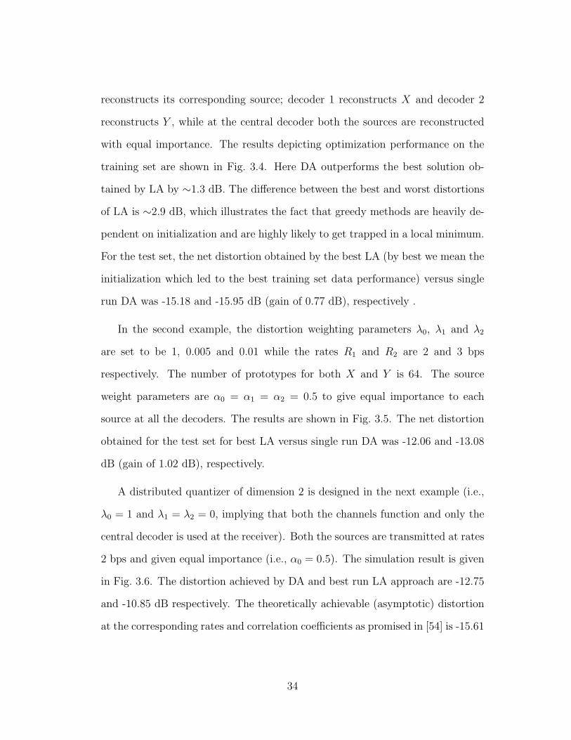
reconstructs its corresponding source; decoder 1 reconstructs X and decoder 2

reconstructs Y , while at the central decoder both the sources are reconstructed

with equal importance. The results depicting optimization performance on the

training set are shown in Fig. 3.4. Here DA outperforms the best solution ob-

tained by LA by ∼1.3 dB. The difference between the best and worst distortions

of LA is ∼2.9 dB, which illustrates the fact that greedy methods are heavily de-

pendent on initialization and are highly likely to get trapped in a local minimum.

For the test set, the net distortion obtained by the best LA (by best we mean the

initialization which led to the best training set data performance) versus single

run DA was -15.18 and -15.95 dB (gain of 0.77 dB), respectively .

In the second example, the distortion weighting parameters λ0, λ1 and λ2

are set to be 1, 0.005 and 0.01 while the rates R1 and R2 are 2 and 3 bps

respectively. The number of prototypes for both X and Y is 64. The source

weight parameters are α0 = α1 = α2 = 0.5 to give equal importance to each

source at all the decoders. The results are shown in Fig. 3.5. The net distortion

obtained for the test set for best LA versus single run DA was -12.06 and -13.08

dB (gain of 1.02 dB), respectively.

A distributed quantizer of dimension 2 is designed in the next example (i.e.,

λ0 = 1 and λ1 = λ2 = 0, implying that both the channels function and only the

central decoder is used at the receiver). Both the sources are transmitted at rates

2 bps and given equal importance (i.e., α0 = 0.5). The simulation result is given

in Fig. 3.6. The distortion achieved by DA and best run LA approach are -12.75

and -10.85 dB respectively. The theoretically achievable (asymptotic) distortion

at the corresponding rates and correlation coefficients as promised in [54] is -15.61

34

−20 −19 −18 −17 −16 −15 −14 −13−23

−22

−21

−20

−19

−18

−17

−16

Distortion of source X (Dx) (in dB)

Dis

tort

ion

of s

ourc

e Y

(D

y) (in

dB

)

LA ApproachDA Approach

Figure 3.4. Comparison between LA and DA approaches for R1 = 3 , R2 = 4, K

= 64, L = 128, α0 = 0.5, α1 = 1, α2 = 0, λ0 =1, λ1 = λ2 = 0.01. Net distortion

from DA is -16.98 dB while LA gives best and worst distortion as -15.69 and

-12.77 dB, respectively. For ease of comparison, a line along which constant Dnet

= -16.98 dB is drawn.

dB.2 Here the DA approach is roughly 2.86 dB away from the asymptotic bound

of the distortion and the greedy LA approach is a further 1.9 dB away. Note that

the distortion from the LA and DA approaches can be further reduced if entropy

coding is employed or the dimension of the quantizers is increased.

In the next example (see Fig. 3.7)), X and Y are drawn from a mixture of four

joint Gaussians. Such a situation can arise, for example, when sources correspond

to the temperature and humidity readings and the different mixture components

are due to varying underlying conditions such as the time of day, pressure, etc.

2To calculate the distortion bounds from [54], we have assumed that the individual sourcedistortions will be approximately the same and hence equal to the average distortion, sinceboth the sources have similar statistics, are encoded at the same rate, and are given equalimportance at the decoder.

35

−16 −15.5 −15 −14.5 −14 −13.5 −13 −12.5 −12−18

−17.5

−17

−16.5

−16

−15.5

−15

−14.5

−14

Distortion of source X (Dx) (in dB)

Dis

tort

ion

of s

ourc

e Y

(D

y) (in

dB

)


Figure 3.5. Comparison between LA and DA approaches for R1 = 2, R2 = 3, K

= L = 64, α0=α1=α2= 0.5, λ0 =1, λ1 = 0.005 , λ2 = 0.01. Net distortion from

DA is -13.44 dB while LA gives best and worst distortion as -12.18 and -10.54 dB,

respectively. For ease of comparison, a line along which constant Dnet = -13.44

dB is drawn.

Here λ1 = λ2 = 0, α0 = 0.5 and the source rates are 3 bps. In our simulations,

the mixtures components are assumed to be equiprobable. The means for X,

Y and correlation coefficients for the four components are taken as {0, 0, 0.87},{1, 0.5, 0.9}, {-1, 1, -0.92} and {2, -1, -0.95} respectively. The variance of X

and Y in all the components of the mixture was taken to be 1. The distortion

values achieved by DA and from the best and worst LA algorithm are −13.59,

−12.74 and −9.87 dB (DA gains 0.85 dB and 3.72 dB over best and worst LA) ,

respectively.

The next simulation result (see Fig. 3.8), depicts the variation in weighted

distortion for the LA (best of 20 runs) and DA approaches for a scalar RDVQ

36

−13.5 −13 −12.5 −12 −11.5 −11 −10.5 −10 −9.5 −9−13.5

−13

−12.5

−12

−11.5

−11

−10.5

−10

−9.5

Distortion of source X (in dB)

Dis

tort

ion

of s

ourc

e Y

(in

dB

)


Figure 3.6. Comparison between LA and DA approaches for a distributed vector

quantizer of dimension 2. R1 = R2 = 2, K = L = 128, α0 = 0.5, λ0 =1,

λ1 = λ2 = 0. Net distortion from DA is -12.75 dB while LA gives best and

worst distortion as -10.85 and -10.01 dB, respectively. For ease of comparison, a

line along which constant Dnet = -12.75 dB is drawn. Achievable distortion as

promised in [54] is -15.61 dB.

system with the number of prototypes for the sources. Here λ0 = 1, λ1 =

λ2 = 0.01 and α0 = α1 = α2 = 0.5 and the source rates R1 and R2 are kept

fixed at 3 bps. As the number of prototypes is increased, the WZ mappings

can possibly combine more non-contiguous regions together and utilize the inter-

source correlation more efficiently. Note that even for large number of prototypes

the greedy LA approach underperforms the DA approach, justifying the use of

a global optimization tool for a robust distributed quantizer design. Also, after

a point increasing the number of prototypes does not lead to reduction in the

distortion cost. This implies that only sufficiently large number of prototypes (in

37

−15 −14 −13 −12 −11 −10 −9−13.5

−13

−12.5

−12

−11.5

−11

−10.5

−10

−9.5

Distortion of source X (in dB)

Dis

tort

ion

of s

ourc

e Y

(in

dB

)


Figure 3.7. Comparison between LA and DA approaches for a distributed vector

quantizer for sources coming from a gaussian mixture model. R1 = R2 = 3 ,

K = L = 64, α0 = 0.5, λ0 =1, λ1 = λ2 = 0. Net distortion from DA is -13.59

dB while LA gives best and worst distortion as -12.74 and -9.87 dB, respectively.

For ease of comparison, a line along which constant Dnet = -13.59 dB is drawn.

comparison to the transmitted indices) are required for achieving a good system

performance.

Finally a note on system complexity. The design complexity of DA-based

algorithm is higher than that of the LA approach. In our simulations, the DA

approach took on an average 20-25 times longer time than for a single run of LA

approach. The run time of the DA algorithm can be further reduced by simple

schemes outlined in [37]. For completeness, we just outline a simple procedure to

accelerate the DA algorithm. In DA, almost all the interesting activity happens

near the phase transitions, when the codevectors split and move to different lo-

cations to minimize the cost. In between the phase transitions, the codevectors

38

remain at the same locations and the changes in distortion cost are insignificant.

Thus, the cooling between phase transitions can be done in a rapid fashion with-

out actually compromising the algorithm performance. We have not pursued the

above idea for accelerating the DA approach in between the phase transitions in

this work and have used the simple exponential cooling schedule for DA. Further,

instead of starting from a high temperature, DA algorithm can be initialized from

a temperature slightly above the critical temperature for first phase transition,

since above this temperature there is only one global minimum on the cost sur-

face (see the result for critical temperature for first phase transition in Appendix).

Note that the design complexity of DA is a one time cost only. During operation

hard quantizers are used and both the DA and LA approaches have the same

operational complexity.

10 20 30 40 50 60 70−15.5

−15

−14.5

−14

−13.5

−13

−12.5

−12

Number of Prototypes

Wei

ghte

d D

isto

rtio

n (in

dB

)


Figure 3.8. Comparison between LA and DA approaches when the number of

source prototypes are varied for R1 = R2 = 3 α0 = α1 = α2 = 0.5; λ0 =1,

λ1 = λ2 = 0.01.

39

3.5 Conclusions

In this chapter, we have proposed a multiple prototype based deterministic

annealing approach for the design of quantizers for a robust distributed source

coding system. The approach is general and is applicable to a wide gamut of cod-

ing and quantization problems such as multiple descriptions, distributed source

coding, CEO problem etc. The approach assumes no prior knowledge about the

underlying probability distribution of the sources, eliminates the dependence on

good ad-hoc initial configurations and avoids many poor local minima of the

distortion cost surface. The necessary conditions (and update equations) for sys-

tem design are derived and presented. Simulation results comparing DA with an

iterative Lloyd-like algorithm are shown. Significant improvements confirm the

advantage of using a global optimization scheme such as DA for robust distributed

vector quantizer design.

40

Chapter 4

Scalable coding of correlated

sources

In this chapter, we consider the problem of scalable distributed coding of

correlated sources that are communicated to a central unit. The general set-

ting is typically encountered in sensor networks. The communication channels

in a sensor field may vary in capacity due to the presence of obstacles or other

phenomena such as fading. In such a scenario, it will be beneficial to convey a

minimal amount of information even when the channel deteriorates. This mo-

tivates the problem of scalable distributed source coding (S-DSC) or successive

refinement of distributed correlated sources, which generalizes the traditional

problem of scalable coding of single source [11, 22, 35, 52]. Successive refinement

for Wyner-Ziv coding (side information at the decoder) was proposed in [49], and

has been studied in [49, 50] from the information-theoretic perspective of char-

acterizing achievable rate-distortion regions. Here we derive practical iterative

41

algorithms for the design of successive-refinable system within the multi-terminal

(distributed) setting, i.e., for a S-DSC system. The general S-DSC problem sub-

sumes several important special cases such as multiple-description coding [29],

robust distributed coding [5, 6, 18] etc.

Various scalability structures for S-DSC may be implemented, such as tree-

structured quantizers or multi-stage quantizers [17]. In practice, multi-stage

structures are often preferred due to their reduced encoding and decoding com-

plexity, and training data requirements. An example is speech coding applications

where multi-stage vector quantizers are heavily used. In this work we first ana-

lyze the design of multi-stage distributed source coding (MS-DSC) [42, 46] and

then the unconstrained scalable distributed coding problem [42, 43]. It may be

tempting to assume that simple combination of algorithms for distributed coding

([13, 34, 40]) and multi-stage quantizer design ([17]), would yield a good MS-DSC

coding scheme. However, as we will see, there exists a fundamental tradeoff be-

tween exploiting inter-source correlation at the base or intermediate layers, and

better reconstruction in subsequent layers of the MS-DSC. Moreover, by allowing

for a slight but controlled mismatch between encoder and decoder estimates and

reconstructions, inter-source correlation can be exploited more effectively.

Next, we consider the unconstrained scalable distributed coding problem. Al-

though a standard ‘Lloyd-style’ distributed coder design algorithm can be gener-

alized to scalable distributed coding, the resulting algorithm depends heavily on

initialization and will virtually always converge to a poor local minimum on the

distortion-cost surface. We propose an efficient initialization scheme for such a

system, which employs a properly designed multi-stage distributed coder.

42

X11, Y11

w

w

w

...........................................................................................................................................................................................................................................................................................................................................................................................................................................................................................................................................................

......................................................................................................................................................................................................................................................................................................................................................................................................................................................................................................................................................................................................................................................................................

..........................................................................................................................................................................................................................................................................................................................................................................................................................................................................................................................................................................................................................................................................................................................................................................................................................................................................................................................

..................................................................................................................................................................................................................................................................................................................................................................................................................................................................................................................................................................................................................................................................

......................................................................................................................................................................................................................................

......................................................................................................................................................................................................................................

...........................................................................

.............................................................................................................................................................................................................................................................................................................................................................................................................................................................................................................................................................................................................................

.......................................................................................................................................................................................................................................................................................................................................................................................................................................................................................................................................................................................................................................................................................................................................................................................................................................

.............................................................................................................................................................................................................................................................................................................................................................................................................................................................................................................................................................................................................................

..................................................................................................................................................................................................................................................................................................................................................................................................................................................................................................................................................................................................................................................................................................................................

...................................................................................................................................................................................................................................................................................................................................................................................................................................................................................................................................................................................

....................................

....................................

....................................

....................................

....................................

....................................

....................................

....................................

....................................

....................................

....................................

....................................

....................................

....................................

....................................

....................................

.............

.............................................................................................................................................................................................................................................................................................................................................................................................................................................................................................................................................................................................................................................................................................................................................................................................................................................................................................

................................................................................

................................................................................

................................................................................

................................................................................

................................................................................

................................................................................

Decoder D00

Decoder D01

Decoder D10

Decoder D11

i1 ∈ {1..2R1x}

Encoder Ey

Encoder Exi2 ∈ {1..2R2x}

j1 ∈ {1..2R1y}

j2 ∈ {1..2R2y}

X

Y

X00, Y00

X01, Y01

X10, Y10

w

Figure 4.1. Scalable distributed source coding

It is also desirable that the S-DSC system be robust to fades or failures of

various communication channels, and utilize all received information to attain

maximize efficiency. We incorporate system robustness objectives by adopting

techniques for robust distributed coder design [40].

4.1 Problem statement and special cases

Consider the S-DSC scenario in Fig. 4.1. For brevity, we will restrict the

analysis to the case of two sources and to two-layers, but without loss of generality

as the model is trivially extendible to an arbitrary number of sources or layers.

Here (X,Y ) are two continuous amplitude, i.i.d., correlated (scalar or vector)

sources. The encoder Ex for source X compresses the data and transmits an index

pair {i1, i2} where i1 ∈ {1..2R1x} and i2 ∈ {1..2R2x}. Similarly the encoder Ey for

Y has an index pair {j1, j2} as output where j1 ∈ {1..2R1y} and j2 ∈ {1..2R2y}.

43

R1x and R1y correspond to the first (base) layer rates while R2x and R2y denote

the incremental second (enhancement) layer rates.

We assume that the fusion center obtains full information from the base layer

while data from the enhancement layers for sources X and Y is lost independently

with probabilities px and py, respectively. Depending on the sub-set of informa-

tion received from the source enhancement layers, the fusion center uses decoder

D00, D01, D10 or D11 to reconstruct X as X00, X01,X10 or X11, respectively and

similarly for Y (see Fig. 4.1). The sub-scripts in a decoder indicate whether

the enhancement layer information for source X and Y have been received, e.g.,

decoder D10 is used when only enhancement layer information from X is received.

Thus the decoders D00, D01, D10 and D11 are used with probabilities p00 = pxpy,

p01 = px(1− py), p10 = (1− px)py and p11 = (1− px)(1− py), respectively.

The distortion incurred when decoder D00 is used for reconstructing sources

will be:

E[αd(X, X00) + (1− α)d(Y, Y00)], (4.1)

where d(·, ·) is an appropriately defined distortion measure and α ∈ [0, 1] is a

weighting factor which governs the relative importance of the sources X and Y

at the fusion center. Distortion terms when decoders D01, D10 or D11 are used

are similarly defined. Note that we use uppercase letters for a random variable

and lowercase letters to denote its particular realization.

We use the following stream-lined notation to denote the distortion terms for

44

a data point (x,y) when different decoders are used:

D00(x, y) = αd(x, x00(i1, j1)) + (1− α)d(y, y00(i1, j1)),

D01(x, y) = αd(x, x01(i1, j1, j2)) + (1− α)d(y, y01(i1, j1, j2)),

D10(x, y) = αd(x, x10(i1, j1, i2)) + (1− α)d(y, y10(i1, j1, i2)),

D11(x, y) = αd(x, x11(i1, j1, i2, j2)) + (1− α)d(y, y11(i1, j1, i2, j2)). (4.2)

where the index pairs are determined by the source values, Ex(x) = {i1, i2} and

Ey(y) = {j1, j2}. In the above expressions, D00 denotes the distortion for a par-

ticular source pair (x,y) when decoder D00 is used and so on. Also for simplicity,

we assume that the weighting factor α is same when different decoders are used.

This simplifying assumption can easily be eliminated by simple modification of

the weight factors in the various distortion terms.

Next we define the net average distortion incurred for a source pair {x,y} as:

Dnet(x, y) = p00D00(x, y) + p01D01(x, y)

+ p10D10(x, y) + p11D11(x, y). (4.3)

The S-DSC design objective is to minimize the following distortion cost given

rate allocations R1x, R2x, R1y and R2y; and enhancement layer loss probabilities

px and py:

E[Dnet(X,Y )]. (4.4)

4.1.1 Special Cases

The S-DSC problem is very general and includes a large number of source

coding problems as special cases. We mention a few of these:

45

1. Single Source Vector Quantizer : If the second source Y does not transmit

any information, and the source X transmits only base layer information,

the problem reduces itself to that of a single source vector quantizer.

2. Distributed Source Coding : In the case when enhancement layer from both

the sources is missing (when px = py =1 or when there is no enhancement

layer transmission (R2x = R2y = 0 bits), the problem reduces to that of

typical distributed source coding.

3. Scalable Coding of a Single Source: When only a single source is present,

the S-DSC problem reduces to scalable coding of a single source.

Next we consider some other special cases where the base layer information

is also allowed to be lost (Note that in this work our assumption of base

layer being always received is for presentation simplicity and the proposed

model can easily be generalized to the most general scenario where base

layer information can be lost.)

4. Scalable Multiple Descriptions Coding : When the two sources X and Y are

identical, and the base layer may also experience loss, the S-DSC problem

reduces to scalable multiple descriptions coding.

5. Multiple Description Coding : This is a special case of scalable multiple

descriptions coding problem when only the base layer information is being

transmitted.

6. Robust Distributed Source Coding : In the general case when sources X and

Y are not identical and the enhancement layer from both the sources is

missing, the problem reduces to robust distributed source coding [6],[40].

46

Here the objective is to reconstruct the sources based on the available num-

ber of descriptions.

We begin our discussion of S-DSC design by first considering a MS-DSC sys-

tem. We highlight the major conflict that happens when distributed coding is

naively combined with multi-stage coding and an approach to resolve the con-

flict. We then propose an iterative design algorithm for the MS-DSC design that

efficiently exploits the inter-source correlation. The next section explains the

functioning of various modules of the MS-DSC system.

4.2 Multi-stage distributed source coding

4.2.1 Encoder

The MS-DSC encoder for source X is shown in Fig. 4.2. The overall encoder Ex

consists of two stage encoders E1x and E2x. Input X is fed to the first stage (base-

layer) encoder E1x whose output is an index i1 and an encoder reconstruction value

Xenc. The residual, ex = X − Xenc is input to the second stage (enhancement

layer) encoder E2x, whose output is an index i2. Since the sources X and Y

are correlated, the encoders E1x and E2x will differ from the nearest-neighbor

quantizers encountered in single-source multi-stage quantization.

Base layer encoder Ex consists of a high rate quantizer (used primarily to

discretize the source) which maps source X to index k1 representing Voronoi

region Cxk1

. The WZ mapping block, employed next, takes in k1 and outputs

index i1 = v1(k1) representing region Rxi1

=⋃

k1:v1(k1)=i1Cx

k1, to be transmitted

47

Base layer encoder E1x

................................................................................

................................................................................

................................................................................

................................................................................

................................................................................

................................................................................

................................................................................

................................................................................ ................................................................................

2313

C1

Quantizer

High Rate

Xi2

i1

+

+

− ex E2x

k1 Xenc

WZ Mapping

1 2 1

........

................................

........................................................................................................................................................................................

Figure 4.2. MS-DSC encoder and an example of Wyner-Ziv mapping from

Voronoi regions to (transmitted) indices

over the channel. An example of WZ mapping for a scalar source with K1 = 7 and

I1 = 3 was given in previous chapter and again reproduced here for convenience

in Fig. 4.2.

The encoder codebook C1 takes index k1 as input and outputs Xenc which is

used to compute the residual ex. Base layer encoder E1y for source Y is defined

similarly. Since the error residuals ex and ey obtained by the first encoding stage

are correlated, a distributed coder should be designed to exploit inter-source

correlations. The second stage encoders E2x and E2y similarly consist of a high

rate quantizer followed by WZ mapping. Since the second stage is the last stage

in our setting here, no encoder codebook is needed in E2x or E2y (in general all

except the last MS-DSC stage encoders contain an encoder codebook as in E1x ).

48

i2j1 C2X00

................................................................................

................................................................................

i1

........

................................

........................................................................................................................................................................................

................................................................................

................................................................................

................................................................................

................................................................................

................................................................................

................................................................................

Decoder D00 for X Decoder D10 for X

C4

C3X10,dec

i1

j1

X10ex,10+

................................................................................

Figure 4.3. MS-DSC decoders D00 and D10 for source X

4.2.2 Decoder

The MS-DSC system consists of four decoders (see Fig. 4.1), depending on

whether the enhancement layers from sources X and Y are received or not. De-

coder D00 is used when only indices i1 and j1 are received and actually comprises

of decoders Dx00 and Dy

00 for sources X and Y , respectively. Both Dx00 (see Fig. 4.3)

and Dx00 just consist of a single codebook as reconstruct X and Y as X00 and Y00,

respectively.

Decoder Dx10 (part of D10) comprises of two codebooks (Fig. 4.3). Similar to

single-source multi-stage coding, the decoding is performed in an additive fashion.

X10,dec is calculated based on indices i1 and j1 using a decoder helper codebook

C3 while the estimate for error residual ex is calculated as ex,10 based on i2 using

a residual codebook C4 as shown. The source reconstruction is obtained as:

X10 = X10,dec + ex,10 (4.5)

Note that the various entities Xenc, X10 and X10,dec (corresponding to D10)

differ in general. In brief, these entities can be interpreted as follows:

1. X10,dec is the decoder helper codebook output based on i1 and j1 and its

49

sole objective is to aid in the reconstruction via (4.5).

2. Xenc, based on k1 is an encoder estimate of X at the base layer in order to

derive the residual for the enhancement layer.

3. X10 is the final source reconstruction values at decoder D10.

The functioning of the other decoders D01 and D11 is similar and other entities

such as X01,dec, ex,01, X01 etc. are analogously defined. For the second source Y ,

we have a similar decoding procedure.

4.2.3 Components to optimize

The design algorithm for MS-DSC system needs to optimizes the high rate

quantizers, WZ mappings (or encoder), encoder and decoder codebooks for all lay-

ers and all sources. We will restrict the scope here to the design of all codebooks

and WZ mappings. (For simplicity, we will assume that high rate quantizers are

independently designed using standard Lloyd’s algorithm [26]. Additional gains

due to their joint optimization with the rest of the system are expected to be

small).

4.2.4 Naive design scheme

We first discuss the design scheme which emerges when distributed coding is

directly combined with multi-stage coding. As it ignores the potential conflict

in objectives we refer to it as “naive” design. In the naive scheme, a base layer

distributed coder is designed while ignoring the enhancement layer and the role

50

of px and py to minimize the following base-layer distortion:

E[αd(X, X00) + (1− α)d(Y, Y00)]. (4.6)

The Wyner-Ziv mappings and the decoder codebook (C2) for the base layer for

both the sources are designed using a standard distributed coder design algorithm

such as in [40, 34]. Consequently, the estimates Xenc at the encoder and X01,dec,

X10,dec and X11,dec for decoders D01, D10 and D11, respectively are calculated only

based on index i1. Note that there is no encoder-decoder mismatch in this scheme

and Xenc(i1) = X01,dec(i1) = X10,dec(i1) = X11,dec(i1) = E[X|X ∈ Rxi1], i.e., the

estimates are simply calculated as the centroids of the region Rxi1

corresponding to

index i1. The encoder codebook C1 and decoder helper codebook C3 for D10 (and

similarly for D01 and D11) are same and solely based on the common information

at both the encoder and decoder, i.e., index i1.

The residual ex is calculated as ex = X − Xenc and similarly for ey. The

resulting training set for {ex, ey} is used to design a distributed coder for the

enhancement layer to minimize the expected distortion corresponding to the last

three distortion terms in (4.4) using a Lloyd-style algorithm for robust distributed

coder design [40] in which the various codebooks and enhancement layer Wyner-

Ziv mappings are optimized given the fixed base layer coder. For more details on

robust distributed coder design, we refer the reader to [38, 40].

4.2.5 Comments on naive design scheme

In essence, the naive scheme for MS-DSC design tries to first minimize the

base layer distortion term by designing a base layer distributed coder. Given

the fixed base layer distributed coder, a robust distributed coder is designed (the

51

term robust distributed coder is used because the enhancement layer channels for

the two sources can fail independently and a particular decoder is used depending

on the available information) to minimize the remaining distortion terms. The

inherent assumption is that ignoring (a) the enhancement layer during base layer

distributed coder design and (b) the role of px and py may not degrade the

performance substantially. For example, when enhancement layer from both

sources is almost always received, px and py are close to 0 implying that the base

layer decoder D00) will be used with very less probability p00 = pxpy. This implies

that the base layer distributed coder design should not be done independently by

ignoring the effect of enhancement layer.

Further to avoid any potential mismatch, only index i1 (available at both

the encoder and decoder) is used as input for the encoder and decoder helper

codebooks and information from other source Y (in the form of index j1) is

ignored.

4.3 Multi-stage distributed coding design algo-

rithm

4.3.1 Motivation and design

The most fundamental deviation of this work from the “natural” approach to

MS-DSC is in the use of different codebooks for constructing Xenc at the encoder

and X01,dec, X10,dec and X11,dec at the decoder. In the sequel we will only mention

X10,dec (Discussion about X01,dec and X11,dec is similar.). At the decoder, both

52

indices i1 and j1 can be utilized to construct X10,dec. However, the encoder for

source X only has access to index i1 to construct Xenc, and does not know j1.

Obviously, there will be a mismatch between Xenc and X01,dec. A possible way

to match X01,dec with Xenc will be to make both X01,dec and Xenc a function of

i1 alone (as was done in the naive approach). But this may actually worsen the

performance of the enhancement-layer distributed coder. For example, consider

a (scalar) source point in the X space (see example of Wyner-Ziv mapping in

Fig. 4.2) lying in the second region and being mapped to index i1 = 2. The

encoder estimate Xenc corresponding to this point may actually lie in the middle

of the line (since it will be calculated as the average of all source points X in

the second and seventh region of high-rate quantizer output that get mapped to

index 2). Obviously the estimate Xenc will be coarse and the error residuals ex

(and similarly for ey) will have higher magnitude (l2-norm for vector sources).

The idea, is therefore to allow for some mismatch between the first (or inter-

mediate) layer estimates at the encoder and decoder and optimize so that efficient

distributed coding at second (respectively next) layer will more than compensate

for any allowed mismatch. Another crucial point to note is that, the source en-

coder has complete knowledge of the source itself or effectively index k1 (which

is the output of the high resolution quantizer used primarily to discretize the

source), while the decoder has additional knowledge from the correlated source

Y , in the form of index j1. This implies that there may exist some (elusive)

additional information at both ends that could be exploited, if an appropriate

means were devised. Also joint design of the distributed coders at both the layers

should be performed (so that impact of enhancement layer and role of px and py

is not neglected while designing base layer distributed coder).

53

We therefore use different codebooks for calculating X10,dec and Xenc at the

decoder versus encoder. The encoder codebook (C1) can have k1 as input, and

the decoder helper codebooks have inputs i1 and j1. This flexibility enables opti-

mization of the tradeoff between better exploitation of inter-source correlations

at the sub-sequent layer, and the cost of some mismatch in the system. Appro-

priate design of encoder and decoder codebooks (as well as WZ mappings) will

optimize the precise overall performance while accounting for the mismatch.

Note that the scheme subsumes single source multi-stage quantizer design

as a special case. Also, when the sources X and Y are uncorrelated, then WZ

mappings for the base layer will converge to a union of contiguous cells (the

encoder E1x will act as a fine-coarse quantizer) and both the encoder and decoder

helper codebooks will effectively be the same and depend on i1 only.

4.3.2 Update rules for proposed MS-DSC algorithm

Herein we assume squared error distortion measure for simplicity. To mini-

mize the cost in (4.4), the Wyner-Ziv mappings and the various codebooks are

optimized iteratively using the following necessary update rules:

1. First Layer Decoder Codebook (C2, at D00):

x00(i1, j1) = arg minφ

∑

(x,y)∈Ri1×Rj1

d(x, φ). (4.7)

2. Second Layer Decoder Codebooks (for residuals, at decoders D01, D10

and D11)

54

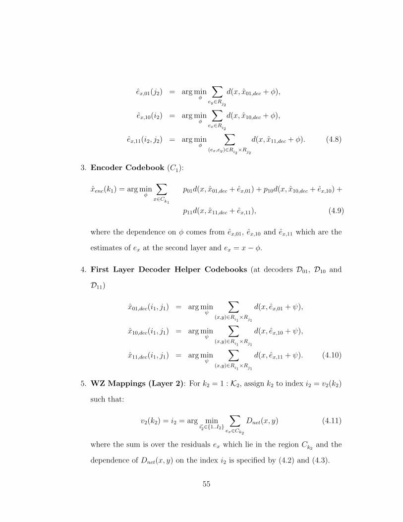
ex,01(j2) = arg minφ

∑ey∈Rj2

d(x, x01,dec + φ),

ex,10(i2) = arg minφ

∑ex∈Ri2

d(x, x10,dec + φ),

ex,11(i2, j2) = arg minφ

∑

(ex,ey)∈Ri2×Rj2

d(x, x11,dec + φ). (4.8)

3. Encoder Codebook (C1):

xenc(k1) = arg minφ

∑x∈Ck1

p01d(x, x01,dec + ex,01) + p10d(x, x10,dec + ex,10) +

p11d(x, x11,dec + ex,11), (4.9)

where the dependence on φ comes from ex,01, ex,10 and ex,11 which are the

estimates of ex at the second layer and ex = x− φ.

4. First Layer Decoder Helper Codebooks (at decoders D01, D10 and

D11)

x01,dec(i1, j1) = arg minψ

∑

(x,y)∈Ri1×Rj1

d(x, ex,01 + ψ),


∑

(x,y)∈Ri1×Rj1

d(x, ex,10 + ψ),


∑

(x,y)∈Ri1×Rj1

d(x, ex,11 + ψ). (4.10)

5. WZ Mappings (Layer 2): For k2 = 1 : K2, assign k2 to index i2 = v2(k2)

such that:

v2(k2) = i2 = arg mini′2∈{1..I2}

∑ex∈Ck2

Dnet(x, y) (4.11)

where the sum is over the residuals ex which lie in the region Ck2and the

dependence of Dnet(x, y) on the index i2 is specified by (4.2) and (4.3).

55

6. WZ Mappings (Layer 1): For k1 = 1 : K1, assign k1 to index i1 = v1(k1)

such that:

v1(k1) = i1 = arg mini′1∈{1..I1}

∑x∈Ck1

Dnet(x, y) (4.12)

Again the dependence of Dnet(x, y) on the index i1 is specified by (4.2) and

(4.3).

The update rules for the second source Y are straightforward to specify from the

above. Also, to reduce clutter, superscripts and arguments were omitted where

obvious, e.g., Ri1 rather than Rxi1; ex,11 rather than ex,11(i2, j2) etc.

4.4 Scalable distributed source coding

In the general setting for the S-DSC problem (see Fig. 4.1), encoders for

sources X and Y transmit index pairs {i1, i2} and {j1, j2}, respectively. The

encoding comprises of directly generating an index pair ({i1, i2} for source X)

rather than source quantization followed by error residual quantization. Similar to

MS-DSC, decoder D00 consists of a single codebook (per source) and takes indices

i1 and j1 as input to obtain the reconstruction X00 (and Y00). The decoders D01,

D10 and D11 also have a single codebook (per source) and decoding is performed

directly using the codebook, rather than in the additive fashion as was being

done in MS-DSC. A block diagram depicting the S-DSC encoder Ex and decoders

D00 and D01 (for X) is shown in Fig. 4.4

Obviously the S-DSC system in its general setting will perform better than

its special constrained case MS-DSC. Also, there is no direct conflict between the

56

k

................................................................................

................................................................................

................................................................................

................................................................................

................................................................................

................................................................................

................................................................................

................................................................................

................................................................................

................................................................................ ..

................................................................................ ................................................................................

Decoder D10Decoder D00

C6C5

i2

j1

j1

i1i1

X10X00

XHigh Rate

Quantizer

{i1, i2}Wyner Ziv

Mapping

11 12 11 21 22 12 22 21 11

Figure 4.4. S-DSC encoder for source X; an example of Wyner-Ziv mapping from

Voronoi regions to index pair {i1, i2}; and decoders D00 and D10 in S-DSC

objectives of distributed and scalable coding in S-DSC, since the design for all the

stages can be performed simultaneously and there is no feedback (dependence)

for calculating the source error residual for any intermediate stage in S-DSC.

However, in S-DSC the encoding complexity grows exponentially with the

sum-rate of base and incremental enhancement layer, i.e., with 2R1x+R2x for source

X (and similarly for Y ). Note that, earlier for MS-DSC, the encoding complex-

ity was proportional to 2R1x and 2R2x for the base and the enhancement layers,

respectively.

Moreover the total storage required for the various decoder codebooks will

grow more rapidly in S-DSC. For example, in S-DSC the codebook for decoderD11

will have storage proportional to 2R1x+R2x+R1y+R2y where as in MS-DSC the cor-

responding storage for the codebooks is approximately proportional to { 2R1x+R1y

+ 2R2x+R2y } due to the additive nature of decoding (the first term corresponds

to the decoder helper codebook and the second term for the residual decoder

codebook).

57

Apart from the increased encoding and storage requirements, efficient design

of Wyner-Ziv mappings from different prototype regions to indices is important

for good performance of the S-DSC system. The index-assignment problem im-

plicit in WZ mapping is a discrete optimization problem. In the case of S-DSC,

we need to map K different regions to one of the I1 ∗ I2 indices for source X

(see Fig. 4.4). One can generalize a distributed quantizer algorithm (such as

in [40],[34]) for the design of S-DSC system. However, random initialization of

the WZ mapping in the generalized DSC iterative algorithm (described below in

Sec. 4.4.1) generally leads to a poor local minimum. While we do not attempt

a global solution to this index assignment problem, we propose to use an opti-

mized MS-DSC system as an efficient initialization for S-DSC design. Simulation

results confirm that the proposed initialization obtains considerable gains over

uninformed, randomly initialized solutions.

We next describe the locally optimal Lloyd-style algorithm alongwith its up-

date rules for S-DSC. After that we explain how the MS-DSC solution can be

used as an efficient initialization for the S-DSC problem.

4.4.1 Iterative design algorithm

We use similar notation in Sec. 4.2 to denote the various S-DSC modules

(Fig. 4.4). The high-rate quantizer for source X maps the source sample to a

prototype associated with the region Cxk where k ∈ {1..K} and K is the total

number of prototypes. Next the WZ mapping block maps the prototype regions

to an index pair {i1, i2} where {i1, i2} ∈ {1..I1} × {1..I2}. Similar procedure is

performed at the second source encoder and indices j1 and j2 are transmitted for

58

the base and enhancement layer respectively.

We again assume squared error distortion measure for simplicity. To minimize

the cost in (4.4), the WZ mappings and the various decoder codebooks (with some

initialization) are optimized iteratively using the following necessary update rules:

1. Wyner-Ziv Mappings For k = 1 : K, assign k to index pair {i1, i2} such

that:

{i1, i2} = arg mini′1,i′2

∑x∈Ck

Dnet(x, y). (4.13)

Here also the dependence of Dnet(x, y) on the index pair is specified by (4.2)

and (4.3).

2. Decoder Codebook: Reconstruction Values

x00(i1, j1) = E[X|X ∈ Rxi1, Y ∈ Ry

j1]

x01(i1, j1, j2) = E[X|X ∈ Rxi1, Y ∈ Ry

j1,j2]

x10(i1, j1, i2) = E[X|X ∈ Rxi1,i2

, Y ∈ Ryj1

]

x11(i1, j1, i2, j2) = E[X|X ∈ Rxi1,i2

, Y ∈ Ryj1,j2

] (4.14)

Similar rules for the second source Y can be obtained and won’t be reproduced

here. In the above update rules, Rxi1

=⋃

i2Rx

i1,i2and Ry

j1=

⋃j2

Ryj1,j2

.

4.4.2 Effective initialization for S-DSC design

MS-DSC is a special case of S-DSC under additive encoding/decoding con-

straints. The proposed scheme for S-DSC takes the optimal MS-DSC system as

an effective initialization and then removes the structural constraints to apply

the iterative algorithm in Sec. 4.4.1.

59

In the MS-DSC scheme, the source space for X (in base layer) is divided into

K1 different regions. These K1 different regions are mapped to one of the I1

regions via the base-layer WZ mapping. The residual ex = X − Xenc is then

quantized by a high-rate quantizer having K2 different output cells (regions),

which are mapped to one of the I2 different regions via enhancement layer WZ

mapping. Hence during design, all the training point samples for source X are

associated with an index {i1, i2}.

Now consider a sample X corresponding to some high-rate quantizer region

k1 ∈ {1..K1} and WZ mapping region i1. This sample is associated with an

index i2 for the enhancement layer (through ex). We define Cxk (k ∈ {1..K}

and K = K1 ∗ I2 ) as the set of all source points X that lie in the region Cxk1

(corresponding to high rate quantizer output index k1) and Rxi2

(corresponding

to index i2 of the enhancement layer WZ mapping), i.e.,

Cxk = Cx

k1

⋂Rx

i2. (4.15)

Now, each of the regions Cxk is associated to an index pair {i1, i2}. So we

effectively view the X source space as divided into K different regions, each of

which is mapped to one of the index pair {i1, i2} via an implicit S-DSC WZ

mapping v(k) = {i1, i2}. We can use these K regions and WZ mappings as an

initial solution for the S-DSC algorithm in Sec. 4.4.1. A similar construction of

the different regions and WZ mapping is performed for source Y .

Encoding during S-DSC operation

Note that the region Rxi2

in (4.15) corresponding to index i2 (outcome of

enhancement layer WZ mapping) is a union of different possibly, non-contiguous

60

regions. Hence the region Cxk in (4.15) is also a union of different possibly, non-

contiguous regions.

The encoding for a sample X will still be performed in a similar fashion

to encoding in MS-DSC, i.e., for X, find the high rate quantizer region and the

corresponding index k1 and Xenc . Using k1, find the base layer WZ mapping index

i1. Calculate the residual ex = X−Xenc and find the corresponding enhancement

layer WZ index i2. The resulting indices i1 and i2 are then transmitted as base

and enhancement layer information, respectively.


We give several examples to demonstrate the gains of (a) the proposed MS-

DSC scheme which resolves the conflict between distributed quantization and

multi-stage coding and (b) the proposed S-DSC scheme initialized using a prop-

erly designed MS-DSC system over the randomly initialized S-DSC approach. In

all the simulations, sources X and Y are assumed to be jointly Gaussian with

zero means, unit variances and correlation coefficient ρ. The weighting coefficient

α of (4.2) is set to 0.5 to give equal importance to both the sources at the de-

coder. A training set of 10000 scalars is generated. The number of prototypes

is 60 for the high rate quantizers which are designed using Lloyd’s algorithm

[26]. We compare four different schemes (a) separate (single-source) multi-stage

coding in which no distributed coding is performed, (b) randomly initialized S-

DSC system (‘Random S-DSC’), (c) structurally constrained MS-DSC system

(Proposed ‘MS-DSC’), and (d) proposed S-DSC system which is initialized by

MS-DSC (‘Proposed S-DSC’).

61

1 1.2 1.4 1.6 1.8 2 2.2 2.4 2.6 2.8−24

−22

−20

−18

−16

−14

−12

−10

−8

−6

−4

Rate

We

igh

ted

Dis

tort

ion

(in

dB

)

Naive MS−DSCSeparate multi stage codingRandom S−DSCProposed MS−DSCProposed S−DSC

(a)

1 1.2 1.4 1.6 1.8 2 2.2 2.4 2.6 2.8−20

−18

−16

−14

−12

−10

−8

−6

Enhancement layer Rate

We

igh

ted

Dis

tort

ion

(in

dB

)


(b)

1 1.2 1.4 1.6 1.8 2 2.2 2.4 2.6 2.8−22

−20

−18

−16

−14

−12

−10

−8

−6

Base layer rate

We

igh

ted

Dis

tort

ion

(in

dB

)


(c)

Figure 4.5. Performance comparison of naive scheme for MS-DSC, separate (sin-

gle source) multi-stage coding, randomly initialized scalable DSC, proposed multi-

stage DSC, and proposed scalable DSC technique. (a) All the transmission rates

are same and varied; (b) enhancement layer rates are varied (base layer rates

fixed at 2 bits/sample); (c) base layer rates are varied (enhancement layer rates

fixed at 2 bits/sample).

62

0 0.2 0.4 0.6 0.8 1−22

−20

−18

−16

−14

−12

−10

−8

−6

px(=p

y)

We

igh

ted

Dis

tort

ion

(in

dB

)

Separate multi stage codingRandom S−DSCProposed MS−DSCProposed S−DSC

(a)

0 0.2 0.4 0.6 0.8 1−22

−20

−18

−16

−14

−12

−10

−8

−6

px(=p

y)

We

igh

ted

Dis

tort

ion

(in

dB

)


(b)

Figure 4.6. Performance comparison of separate (single source) multi-stage cod-

ing, randomly initialized scalable DSC, proposed multi-stage DSC, and proposed

scalable DSC technique as the probability of enhancement layer loss px(= py) is

varied. All the transmission rates are 2 bits/sample. In (a) inter-source correla-

tion ρ = 0.97 while in (b) ρ = 0.9.

63

0.84 0.86 0.88 0.9 0.92 0.94 0.96 0.98 1−23

−22

−21

−20

−19

−18

−17

−16

−15

−14

−13

Inter−source correlation

We

igh

ted

Dis

tort

ion

(in

dB

)


(a)

0.84 0.86 0.88 0.9 0.92 0.94 0.96 0.98 1−23

−22

−21

−20

−19

−18

−17

−16

−15

−14

−13

Inter−source correlation

We

igh

ted

Dis

tort

ion

(in

dB

)


(b)

Figure 4.7. Performance comparison of separate (single source) multi-stage cod-

ing, randomly initialized scalable DSC, proposed multi-stage DSC, and proposed

scalable DSC technique as the inter-source correlation is varied. All the transmis-

sion rates are 2 bits/sample. The probability of enhancement layer loss px(= py)

is 0.2 in (a) and 0.1 in (b).

64

In the first set of experiments (see Fig. 4.5), we plot the weighted distor-

tion at the decoder in (4.4) vs. rate for the various schemes. The probability

of enhancement layer loss for both sources px = py = 0.2 and ρ = 0.97. In

Fig.(a), the same transmission rate is allocated to each layer of each source, i.e.,

R1x = R2x = R1y = R2y = R. We also plot the performance of naive MS-DSC

scheme in these set of experiments. The proposed MS-DSC scheme achieves sub-

stantial gains of upto 6.8 dB over the naive scheme (at R = log2(3) bits) while

the proposed S-DSC scheme leads to considerable gains over Random S-DSC ap-

proach and gains upto ∼ 3.3 dB are obtained (e.g., at R = log2(5) bits/sample).

Also the performance of naive MS-DSC scheme is even worse than that of sepa-

rate (single source) multi-stage coding, as it ignores the potential conflict between

the objectives of distributed quantization and multi-stage coding. In Fig (b), the

base layer rates R1x and R1y are fixed at 2 bits/sample while the enhancement

layer rate R2x(= R2y) is varied. Again the proposed MS-DSC and S-DSC schemes

outperform their respective counterparts, namely the naive MS-DSC and Ran-

dom S-DSC schemes and gain upto 9 and 2.6 dB respectively at rates 1 and 2

bits/sample respectively. In Fig. (c), the base layer rate R1x(= R1y) is varied

while the enhancement layer rates R2x and R2y are fixed at 2 bits/sample. Here

again the proposed MS-DSC and S-DSC schemes outperform naive MS-DSC and

Random S-DSC scheme and gains upto 7.2 and 2.8 dB respectively at rates log2(7)

and 2 bits/sample, respectively.

In the next set of experiments, we fix all the transmission rates R1x = R2x =

R1y = R2y to be 2 bits/sample. The probability of enhancement layer loss for

both sources px(= py) is varied and the weighted distortion is plotted. In (a), the

inter-source correlation ρ is 0.97 while in (b) ρ is 0.9. Here again the proposed

65

MS-DSC and S-DSC schemes consistently outperform the other schemes.

Next we plot the weighted distortion as a function of inter-source correlation

for two different probability of enhancement layer loss px(= py): 0.2 and 0.1,

respectively. Again all the transmission rates R1x = R2x = R1y = R2y are fixed

at 2 bits/sample. We again find that the proposed MS-DSC and S-DSC schemes

consistently outperform the other schemes. In fact, in all the simulations the

performance of the Random S-DSC algorithm is even worse than MS-DSC most

of the times, which reiterates the importance of an efficient initialization for S-

DSC.

Finally, we note that the proposed methods are extendible to incorporate

entropy coding, but such extension is omitted for brevity. Further for fair com-

parison and to eliminate atypically poor results, the initialization for both the

Random S-DSC and MS-DSC algorithms was done 20 times and the best results

are reported.

4.6 Conclusions

In this chapter, we considered the design of scalable distributed source coders.

The proposed S-DSC system is robust to a partial number of channel failures and

utilizes all the available information to attain the best possible compression effi-

ciency. We first identify the inherent conflict between the objectives of distributed

quantization and multi-stage coding and show how to resolve the conflict in the

MS-DSC system, a special constrained case of the S-DSC problem. Our scheme

allows a controlled mismatch between the encoder and decoder reconstruction for

66

estimating the enhancement layer residual and jointly optimizes all the compo-

nents in the MS-DSC system. Next we show that a Lloyd-style iterative S-DSC

algorithm is heavily dependent on initialization and can even be worse than the

performance of a proposed multi-stage DSC algorithm. The multi-stage DSC

algorithm solution is used as an efficient initialization for the S-DSC design algo-

rithm. Simulation results show that (a) the that the proposed MS-DSC scheme

consistently outperforms other naive schemes and single source (separate) dis-

tributed multi stage coding schemes and (b) proposed S-DSC scheme initialized

using a properly designed MS-DSC system consistently outperforms the randomly

initialized S-DSC approach.

67

Chapter 5

Distributed predictive coding

In this chapter, we discuss distributed coding of correlated sources with mem-

ory. We specifically employ linear predictive coding to exploit the temporal cor-

relations within a source. The prediction errors of the different sources can be

assumed to be typically memoryless. However, they will be correlated since the

original sources themselves were correlated. Thus a distributed quantizer needs

to be designed for the prediction errors to exploit the inter-source correlation. We

reformulate the problem of distributed coding of correlated sources with memory

within the representative setting of distributed predictive coding (DPC).

DPC system design poses major challenges due to the fundamental conflict

between the objectives of distributed quantization and predictive coding. Sim-

ply combining a distributed quantization algorithm with predictive coding leads

to a naive design and severely degrades the prediction loop performance of the

resulting DPC system.

A complementary challenge arises from the instabilities in the design of closed

68

loop predictors, whose impact has been observed in the single source case, but is

greatly exacerbated in the case of DPC. To circumvent the difficulty of closed loop

predictive quantizer design, we derive and adopt a technique called asymptotic

closed loop (ACL). Within the ACL framework, the design is effectively done in

open loop (eliminating issues of error buildup through the prediction loop), while

ensuring that asymptotically, the prediction error statistics converge to closed

loop statistics.

It should be mentioned that the temporal correlations within a source can con-

ceivably be exploited by blocking sources into large vectors, but such a scheme

will have high complexity and will be extremely sensitive to initialization and

poor local optima as we have seen in Chapter 3 and in [38, 39, 40, 51]. Moti-

vated by these observations, a notable approach to predictive coding of correlated

sources has been proposed in [51] where a uniform quantization grid was imposed

on the product space (across sources) of prediction errors, on which the main

support of the joint distribution was identified and a DSC code devised. The

emphasis in that paper’s results was on the design of optimal predictor filters in

such distributed setting and on how they deviate from the case of non-distributed

predictive coding. Also in [58], an algorithm for predictive coding of correlated

sources exhibiting high inter-source correlation was given where different com-

ponents (encoder and decoders) were designed. However in both the previous

settings, neither the optimality of the algorithms was proven nor the system can

be guaranteed to be drift-free for all values of inter-source/temporal correlations.

In this chapter we propose optimal algorithms with ‘zero-drift’ and ‘controlled-

drift’ for distributed predictive coding. The ‘controlled-drift’ algorithm includes

the zero-drift approach as a special case that emerges whenever the impact of

69

potential drift overwhelms the benefits of improved prediction. Both the DPC

schemes also subsume as special extreme cases (a) separate predictive coding of

sources and (b)memoryless distributed coding. We begin the chapter by first

reviewing the different methods used for single-source predictive coding, namely

the open loop (OL), closed loop (CL) and ACL. After that, we discuss the various

DPC design algorithms that we have proposed in [41, 44, 45].

5.1 Predictive vector quantizer design for single-

source

A typical predictive vector quantizer (PVQ) is shown is Fig. 5.1. We assume

that the channel is noiseless and concentrate only on the source coding modules.

Let X be a real valued scalar source {xn}Nn=0. For simplicity, assume that the

source X has zero mean and first-order linear prediction is performed (In general,

X can be a vector and higher order prediction can be performed. For a more

detailed treatment of PVQ, refer [17]). The predictor Px is used to predict the

next source sample as xn+1 = Pxxn. The prediction error at time n + 1 is

calculated as en+1 = xn+1 − xn+1.

The encoder E (of a quantizer Q) takes en as input and outputs an index in =

E(en) to be transmitted over the channel. At the decoder, the error reconstruction

is calculated via a decoder codebook as D(in). A predictive quantizer can be

70

concisely described by the following mathematical operations:

en = xn − xn, (5.1)

in = E(en), (5.2)

xn = xn +D(in), (5.3)

xn+1 = Px xn. (5.4)

Though the encoder E and decoder D are actually needed for implementing

a typical PVQ system, for simplicity an abstraction is made that a quantizer Q

quantizes the prediction error and en = Q(en) = D(E(en)).

The PVQ system design is problematic due to the presence of feedback loop.

A training set of prediction errors is needed for the design of quantizer Q. How-

ever, these prediction errors have themselves to be generated in closed loop and

therefore depend on the quantizer which needs to be designed. This affects the

convergence and stability of the algorithm and the resulting system performance

can be poor. Next we review the various approaches for predictive coding of

single sources and discuss the convergence/stability issues associated with these

approaches.

5.1.1 Open loop approach

A schematic of open loop PVQ design [8] approach is shown in Fig. 5.2. In

OL approach, a training set of prediction errors is generated from the original

sequence of samples directly as follows:

en = xn − Px xn−1. (5.5)

71

D

........

................................

........................................................................................................................................................................................

........

................................

........................................................................................................................................................................................

................................................................................

................................................................................

................................................................................

................................................................................

................................................................................

................................................................................

................................................................................

................................................................................

................................................................................

................................................................................

................................................................................

................................................................................

................................................................................

................................................................................

DelayDelay

Channel

X

−

X

X

P

e

e

i

P

X

X

e

+

+

+E

D

........

................................

........................................................................................................................................................................................

Figure 5.1. Predictive vector quantizer

The quantizer Q is then designed for these fixed prediction errors via Lloyd’s

algorithm [26]. The design procedure is simple and algorithm will converge to a

local minimum on the distortion-cost surface (Thus it is stable). However, during

operation, the PVQ system actually runs in closed loop and the prediction is

actually performed using the source reconstruction X instead of X. Hence the

error statistics differ from those for which the quantizer was designed and the

resulting system performance is sub-optimal.

5.1.2 Closed loop approach

A schematic of closed loop PVQ design [8] approach is shown in Fig. 5.3. Here

p denoted the iteration of the CL approach. The OL design is used to initialize

the quantizer Q(p) at p = 1. Given the initial quantizer, the prediction errors are

actually calculated in closed loop as shown in Figure by the following expression:

en = xn − Px xn−1. (5.6)

The system then iterates in closed loop to generate new training data, for

the redesign of the quantizer, until (hopefully) convergence. However, since the

72

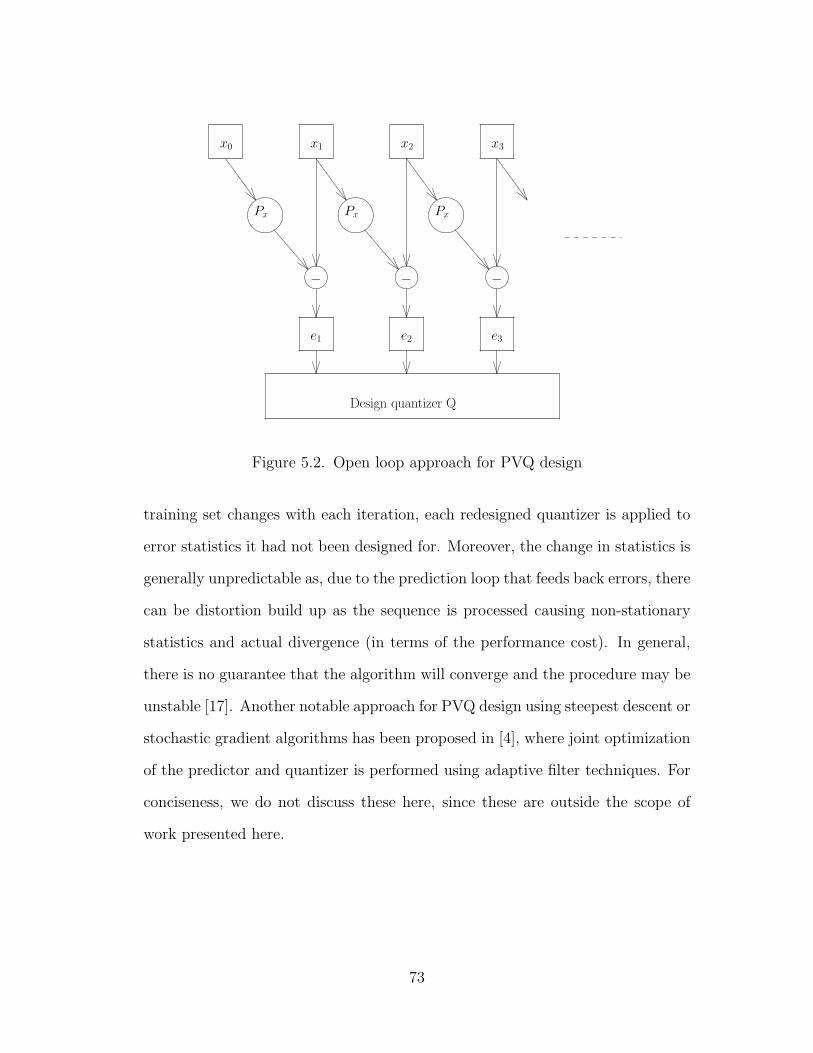
e3

Px

........

................................

........................................................................................................................................................................................ ........

................................

........................................................................................................................................................................................ ........

................................

........................................................................................................................................................................................

........

....................................

......................................

..........................................................................................................................................................................................................................................................................

........

....................................

......................................

..........................................................................................................................................................................................................................................................................

............... ............... ............... ............... ............... ............... .....

.................................................................................................................................................................

................................................................................

.................................................................................................................................................................

................................................................................

.................................................................................................................................................................

................................................................................

.....................................................................................................................................................................

................................................................................

................................................................................ ................................................

................................ ................................................

................................

.................................................................................................................................................................

................................................................................

.....................................................................................................................................................................

................................................................................

.....................................................................................................................................................................

................................................................................

................................................................................ ................................................

................................ ................................................

................................

................................................................................ ................................................

................................ ................................................

................................

Design quantizer Q

x0 x1 x2 x3

Px Px

− − −

e1 e2

........

....................................

......................................

..........................................................................................................................................................................................................................................................................

Figure 5.2. Open loop approach for PVQ design

training set changes with each iteration, each redesigned quantizer is applied to

error statistics it had not been designed for. Moreover, the change in statistics is

generally unpredictable as, due to the prediction loop that feeds back errors, there

can be distortion build up as the sequence is processed causing non-stationary

statistics and actual divergence (in terms of the performance cost). In general,

there is no guarantee that the algorithm will converge and the procedure may be

unstable [17]. Another notable approach for PVQ design using steepest descent or

stochastic gradient algorithms has been proposed in [4], where joint optimization

of the predictor and quantizer is performed using adaptive filter techniques. For

conciseness, we do not discuss these here, since these are outside the scope of

work presented here.

73

e(p)2

Px

........

................................

........................................................................................................................................................................................−

........

....................................

......................................

..........................................................................................................................................................................................................................................................................

Px

........

................................

........................................................................................................................................................................................−

........

................................

........................................................................................................................................................................................ ........

................................

........................................................................................................................................................................................

................................................................................

................................................................................................................................

................................

................................................................................

...............................................................................................

................................................................................

................................................................................

......................................................................................................................................................................................................................................................................................................................................................................................................................................................................................................................................

..............................

..............................

..............................

..............................

..............................

..................

................................................................................

................................................................................

................................................................................

................................................................................

.........................................................................................................................................................

................................................................................

................................................................................

................................................................................

..................................................................................................................................................................................................................................................................................................................................................................................................................................................................................................................................

................................................................................

................................................................................

..............................

..............................

..............................

..............................

..............................

..................

................................................................................

...............................................................................................

................................................................................

................................................................................

................................................................................................................................................

................................................................................

............... ............... ............... ............... .........

Design new quantizer Q(p)

Iteration

Repeat

x0 x1 x2

e(p)1

x(p)0 x

(p)1 x

(p)2

Q(p−1)

+ +

Q(p−1)

........

....................................

......................................

..........................................................................................................................................................................................................................................................................

Figure 5.3. Closed loop approach

5.1.3 The asymptotic closed loop approach

The ACL design approach [19, 20] mitigates the shortcomings related to sta-

bility/convergence in predictive coder design . A subterfuge is employed wherein

the design is effectively performed in open loop, where each quantizer is de-

signed for the statistics of the exact signal it then quantizes to produce a new

sequence of reconstruction for the next iteration, thereby circumventing stability

issues. Asymptotically, the loop is virtually closed in the sense that the design ap-

proaches closed loop statistics despite open loop operation within each iteration.

A schematic of the approach is given in Fig. 5.4.

More specifically, for a given quantizer Q(p−1) and reconstruction sequence

X(p−1) obtained at iteration p− 1, a new training set of prediction errors T (p) =

74

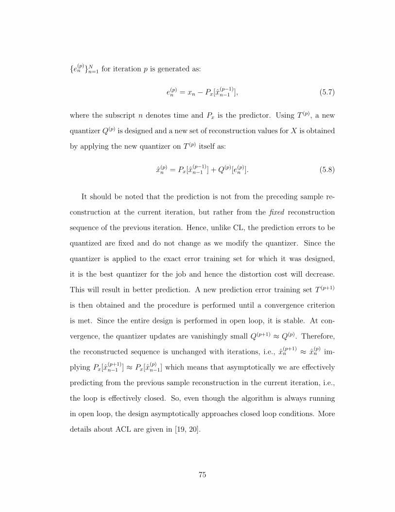
{e(p)n }N

n=1 for iteration p is generated as:

e(p)n = xn − Px[x

(p−1)n−1 ], (5.7)

where the subscript n denotes time and Px is the predictor. Using T (p), a new

quantizer Q(p) is designed and a new set of reconstruction values for X is obtained

by applying the new quantizer on T (p) itself as:

x(p)n = Px[x

(p−1)n−1 ] + Q(p)[e(p)

n ]. (5.8)

It should be noted that the prediction is not from the preceding sample re-

construction at the current iteration, but rather from the fixed reconstruction

sequence of the previous iteration. Hence, unlike CL, the prediction errors to be

quantized are fixed and do not change as we modify the quantizer. Since the

quantizer is applied to the exact error training set for which it was designed,

it is the best quantizer for the job and hence the distortion cost will decrease.

This will result in better prediction. A new prediction error training set T (p+1)

is then obtained and the procedure is performed until a convergence criterion

is met. Since the entire design is performed in open loop, it is stable. At con-

vergence, the quantizer updates are vanishingly small Q(p+1) ≈ Q(p). Therefore,

the reconstructed sequence is unchanged with iterations, i.e., x(p+1)n ≈ x

(p)n im-

plying Px[x(p+1)n−1 ] ≈ Px[x

(p)n−1] which means that asymptotically we are effectively

predicting from the previous sample reconstruction in the current iteration, i.e.,

the loop is effectively closed. So, even though the algorithm is always running

in open loop, the design asymptotically approaches closed loop conditions. More

details about ACL are given in [19, 20].

75

x(p)2

−........................................

........................................................................................................................................................................................−

........

.....................................

...............................................................................................................................................................................................................................................................................................................

Px ............................................

......................................

..........................................................................................................................................................................................................................................................................

Px

........

.................................

...............................................................................................................................................................................................

.................................

.......................................................................................................................................................................................

............... ............... ............... ............... .........................................................................................................................................

................................

........................................................................................................................

................................................................................

.......................................................................................

................................................................................

........................................................................................................................

................................................................................

............................................................................................

................................................................................

................................................................................................................................................................................................................................................................................................................................................................................................................................................................................................................................

................................................................................

...........................................................................................................................................................................................................................................................................................................................................................................................................................................................................................................................

................................................................................

................................................................................ ................................................

................................

................................................................................ ................................................

................................

................................................................................

............................................................................................................................................................................................

...............................

............................................................................................................................................................................................................

....................

..........

................................................................................

................................................................................

................................................................................

................................................................................

Design new quantizer Q(p)

e(p)2

+

e(p)1

x2x1x0

x(p−1)0 x

(p−1)1 x

(p−1)2

Repeat

Iteration

e(p)1 e

(p)2

+

x(p)1

........

................................

........................................................................................................................................................................................

Figure 5.4. Asymptotic closed loop approach

5.2 DPC:Problem statement

Once again consider the simplest distributed source coding scenario of Fig. 5.5.

For brevity, we restrict the presentation to two sources (generalization to an

arbitrary number of sources is straightforward). Here X and Y are two continuous

amplitude, correlated (scalar or vector) sources with memory. The two source

encoders compress and transmit source information at rates R1 and R2 bits per

source sample respectively, to the central unit (joint decoder). The objective is

76

X, Y-

-

-

-

Y Encoder 2

Encoder 1

Decoder

X

-

Figure 5.5. Distributed coding of two correlated sources

to minimize the following expected distortion cost:

D = E{αd(X, X) + (1− α)d(Y, Y )}, (5.9)

where d(·, ·) is an appropriately defined distortion measure, X and Y are the

reconstruction values for X and Y respectively, and α ∈ [0, 1] is a weighting

factor that accounts for the relative importance of the sources at the decoder.

We employ predictive coding to exploit temporal redundancies (We will re-

strict the scope to linear prediction). The prediction errors ex (for X) and ey (for

Y ) will be correlated. Therefore, instead of the standard predictive quantizer, a

distributed quantizer needs to be designed to exploit inter-source correlations.

A mechanism to enable full leveraging of information from another correlated

source requires that the encoder and decoder reconstruction of the prediction

errors differ. We begin by describing the ‘zero-drift’ approach wherein both the

source encoder and decoder have access to exactly the same prediction error re-

construction for the prediction loop and then propose a ‘controlled-drift’ approach

where the constraint of zero-drift is relaxed.

77

5.3 Zero-drift approach

5.3.1 Encoder

The zero-drift distributed predictive encoder for source X is depicted in

Fig. 5.6. The input to the high resolution quantizer Qx is ex = X − Xenc where

Xenc is the predicted value of X at the encoder. Qx maps the prediction error

ex to an index k representing Voronoi region Cxk (a prototype can be associated

with each Voronoi region). The WZ mapping module is employed next. (For

completeness and easy readability, we give a brief description of WZ mapping

here in this chapter as well). The WZ mapping block takes in k and outputs

index i = v(k) for transmission over the communication channel, and which rep-

resents region Rxi =

⋃k:v(k)=i C

xk . The encoder codebook Cenc produces ex,enc, the

prediction error reconstruction value. An example of WZ mapping for a scalar

source with K = 7 and I = 3, is given in Fig. 5.6.

The reconstructed residual ex,enc is added to Xenc to obtain Xenc, the sample

reconstruction value for the encoder prediction loop. A linear predictor Px is

applied to Xenc to predict the next source sample. For Y , we similarly define the

quantizer Qy, regions Cyl and Ry

j . Here, the L Voronoi regions are mapped to

J indices via a WZ mapping w(l) = j. Next, we explain the functioning of the

distributed predictive decoder in the zero-drift setting.

78

Xenc

..

2 3 1 231 1

........

................................

........................................................................................................................................................................................

........

................................

........................................................................................................................................................................................ ...........................

.....................................................

................................................................................

................................................................................

................................................................................

................................................................................

................................................................................

................................................................................

................................................................................

Cenc

High Rate

Mapping

Wyner Ziv

Quantizer

Xkex

+

+

Xenc

Px

-

i ∈ {1..2R1}

ex,enc(i)

................................................................................ ................................................................................

Figure 5.6. Block diagram of a DPC zero-drift encoder and a scalar example of

WZ mapping from prototypes (Voronoi regions) to indices.

Xenc

........

................................

........................................................................................................................................................................................

................................................................................

................................................................................

................................................................................

................................................................................

................................................................................

................................................................................

................................................................................

................................................................................

................................................................................

X

ex

Cenc

Cdec +

+i

Px

j

ex,encXenc

........

................................

........................................................................................................................................................................................

Figure 5.7. DPC zero-drift decoder for source X

5.3.2 Decoder

The decoder module in charge of reproducing X (see Fig. 5.7) receives indices

i and j from sources X and Y respectively. Index i is first used to reconstruct

ex,enc so that the encoder prediction loop can be exactly replicated without error

or potential drift to generate Xenc and Xenc via the predictor Px. Given the index

pair (i, j), the decoder retrieves ex from the decoder codebook , Cdec, and adds it

to Xenc to obtain the decoder reconstruction X.

79

5.3.3 Observations and intuitive considerations

It is important to note that the WZ mappings compromise the quality of

the sample reconstruction in the prediction loop in order to exploit inter-source

correlation and improve the decoder reconstruction. In particular, region Rxi =

⋃k:v(k)=i C

xk is typically formed as a union of distant Voronoi cells Cx

k in the hope

that the information from source Y will allow the decoder to separate them (see

the example WZ mapping in Fig. 5.6). A fundamental tradeoff emerges, as in or-

der to exploit inter-source correlations between ex and ey to better reconstruct the

current sample at the decoder, we compromise the performance of the prediction

loop and hence the quality of future reconstruction.

We should also re-emphasize that Xenc is a (coarse) reconstruction of X which

only serves the prediction loop, and is generally different from X, the decoder

reconstruction of X. Also note that the “encoder codebook” Cenc which is used

in the prediction loop at both the encoder and the decoder is, in general, different

from the “decoder codebook” Cdec (used only at the decoder).

5.3.4 Naive approach for DPC design

One can argue that predictive coding per se is largely a solved problem and

a predictive quantizer module can be straightforwardly integrated with existing

distributed memoryless coding methodologies (such as in [34]) to obtain a DPC

system. The idea in such a naive approach will be to first obtain a set of prediction

error residuals (ex, ey). Let us assume that these are initialized with the open

loop prediction errors. Then a distributed coder will be designed to minimize the

80

following distortion cost between the prediction errors:

E[αd(ex, ex) + (1− α)d(ey, ey)], (5.10)

(see e.g. DSC in [34]) (similar to the practice for traditional single-source pre-

dictive quantizer, wherein the quantizer is designed to minimize the distortion

between prediction error and its reconstruction). This will resemble the open

loop design in traditional single-source predictive coding. For the subsequent

iterations (of closed loop predictive quantizer design) for source X, ex,enc will be

calculated solely based on index i, since this is the only common information

guaranteed to be available at both the encoder and decoder (index j from source

Y is available only at decoder). Next one computes ex,enc(i), corresponding to

transmitted index i as ex,enc(i) = E(ex|ex ∈ Rxi ). Using this, the sequences Xenc,

Xenc and prediction errors ex will be computed in closed loop. The crucial point

to note in such a design is that ex,enc(i) for index i is a very coarse estimate

for ex. For example, in Fig. 5.6, for index i = 2, ex,enc may lie somewhere in

regions in the middle of the line. This will cause the estimate Xenc to be coarse

as well and degrade the performance of the prediction loop. The prediction error

statistics for subsequent samples will differ greatly from those assumed during

the distributed coder design and may even cause instability as will be illustrated

in the results section. This shortcoming is primarily due to neglecting the impact

of the feedback prediction loop during the design of the distributed coder. Hence,

there is a major conflict between the objectives of distributed quantization and

predictive coding, and the corresponding tradeoff should be explicitly optimized.

81

5.3.5 Closed loop vs ACL design

For conceptual simplicity, let us consider first order linear prediction. We note

that the quantized error sample ex,enc at time n impacts the sequence Xenc and

X from time n + 1 onwards due to the presence of the prediction loop. On the

other hand, ex at time n only impacts the current X (at time n), as is explicitly

depicted in Fig. 5.7. Hence, if one tries to directly design a distributed quantizer

for the quantities being quantized, namely, the pair of prediction errors {ex, ey}to minimize the distortion in (5.10), the ultimate end-to-end distortion in (5.9)

will not be minimized.

However, if the DPC decoder were to perform in “open loop” as shown in

Fig. 5.8, then a particular sample of ex,enc will affect only the next sample (in

case of mth order linear predictor, it will affect m future samples) of X and not all

the samples following it. This is our main rationale of adopting the asymptotic

closed loop (ACL) approach [19, 20] for DPC system design, in which the design

iterations are performed in open loop and the prediction loop is essentially closed

asymptotically. The functioning of the ACL based DPC decoder will be explained

in detail in Section 5.4. An important characteristic of the ACL technique is

that the design is performed in open loop but as the algorithm converges, the

prediction loop is effectively closed and the operation mimics closed loop. Next

we explain how the ACL approach for predictive quantizer design can be adapted

for zero-drift DPC design.

82

X(p+1)n+1

........

................................

........................................................................................................................................................................................

................................................................................

................................................................................

................................................................................

................................................................................

................................................................................

................................................................................

................................................................................

................................................................................

................................................................................

P(p)x

X(p)enc,n

j(p+1)n+1

i(p+1)n+1

i(p)n e

(p)x,enc,n

+

+

Cenc

Cdec

e(p+1)x,n+1

X(p)enc,n+1

X(p−1)enc,n

........

................................

........................................................................................................................................................................................

Figure 5.8. DPC zero-drift decoder in open loop during the design phase

5.4 ACL for zero-drift distributed predictive cod-

ing

The ACL distributed predictive decoder (zero-drift approach) for source X

is shown in Fig. 5.8. Here i(p)n , j

(p)n denote the received indices in the pth ACL

iteration. e(p)x,enc,n is the prediction error estimate of the encoder codebook during

iteration p for nth time sample. The other entities X(p−1)enc,n , X

(p)enc,n, etc., are cor-

respondingly defined. During the design iteration, the prediction loop is open as

shown. The distortion cost to be minimized is:

D(p) = E[α d(X, X(p+1)) + (1− α) d(Y, Y (p+1))]. (5.11)

Note that during iteration p, we seek to minimize the ultimate cost at iteration

p+1. Asymptotically, this makes no difference. This setting is used to ensure that

the direct impact of the present error reconstruction (e(p+1)x,n+1), and previous error

reconstruction (e(p)x,enc,n) via the prediction loop on X

(p+1)n+1 is taken into account

for effective update rules. Also, since the design is actually in open loop, e(p)x,enc,n

affects X(p+1) at time n + 1 only.

83

5.4.1 Update rules: zero-drift DPC

For simplicity, we assume that d(·, ·) is the squared error distortion measure.

The decoder codebook, encoder codebook, WZ mappings and the predictor are

updated iteratively using the following steps:

1. Decoder Codebook (Cdec): Entry (i, j), i = 1 : I and j = 1 : J is given

by:

ex(i, j) = arg minφ

∑

n:(e(p+1)x,n ,e

(p+1)y,n )∈Ri×Rj

d(e(p+1)x,n , φ). (5.12)

2. Encoder Codebook (Cenc): Entry i, i = 1 : I is given by:

ex,enc(i) = arg minψ

∑

n:e(p)x,n∈Ri

[α d(e(p+1)x,n+1, e

(p+1)x,n+1)

+(1− α) d(e(p+1)y,n+1, e

(p+1)y,n+1)]. (5.13)

where the resulting prediction error of source X depends on ψ via e(p+1)x,n+1 =

xn+1 − P(p)x [x

(p−1)n + ψ]. Note that e

(p+1)x,n+1 is shorthand for ex(i

(p+1)n+1 , j

(p+1)n+1 ),

the reconstructed value of e(p+1)x,n+1.

3. WZ Mappings: For k = 1, . . . , K, assign k to index i = v(k) such that:

v(k) = arg mini∈{1..I}

∑

n:e(p)x,n∈Ckor

e(p+1)x,n+1∈Ck

[αd(e(p+1)x,n+1, ex(i, j

(p+1)n+1 ))

+(1− α)d(e(p+1)y,n+1, ey(i, j

(p+1)n+1 ))]. (5.14)

4. Predictor: See sub-section 5.4.2.

84

The update rules for WZ mappings, the encoder codebook and the decoder

codebook and predictor for source Y are similarly obtained. Note that i and j

point to codebook entries, subscript n indicates time, and superscript p indicates

the ACL iteration. To reduce clutter, superscripts were omitted where obvious,

e.g., Ri for Rxi .

Further note that for presentation simplicity, we assume the codebooks and

WZ mappings in iteration p and p + 1 are same. Hence the expressions on the

left hand side of the above update rules correspond to encoder codebook (and

respectively decoder codebook and WZ mappings) for both iteration p and p+1.

We then increment the iteration counter p ← p + 2. Note that this notion

of incrementing p by 2 is just for conceptual simplicity and asymptotically (as

p →∞) this will not make any difference.

5.4.2 Predictor optimization

To obtain an effective update rule for the predictor, we keep the various code-

books and WZ mappings fixed and take the partial derivative of the distortion

cost in (5.11) with the predictor. Specifically, we set ∇P

(p)x

D(p) equal to 0.

For the fixed set of reconstructed sequence {x(p−1)enc,n }N

n=0, the prediction error

at iteration p is calculated as:

e(p)x,n = xn − P (p)

x [x(p−1)enc,n−1]. (5.15)

For notational simplicity, we break the distortion cost in (5.11) as D(p) =

αD(p)x + (1 − α)D

(p)y , where D

(p)x and D

(p)y are the contributions to the distor-

tion from sources X and Y , respectively: D(p)x = E[d(X, X(p+1))] and D

(p)y =

85

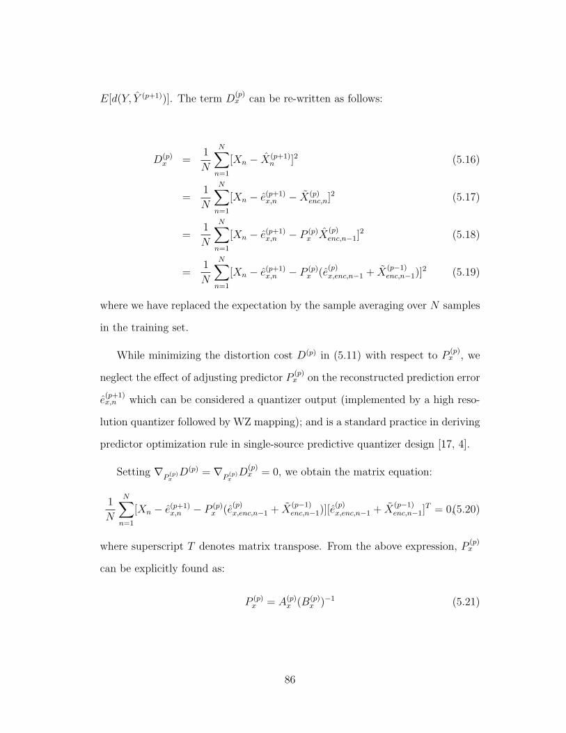
E[d(Y, Y (p+1))]. The term D(p)x can be re-written as follows:

D(p)x =

1

N

N∑n=1

[Xn − X(p+1)n ]2 (5.16)

=1

N

N∑n=1

[Xn − e(p+1)x,n − X(p)

enc,n]2 (5.17)

=1

N

N∑n=1

[Xn − e(p+1)x,n − P (p)

x X(p)enc,n−1]

2 (5.18)

=1

N

N∑n=1

[Xn − e(p+1)x,n − P (p)

x (e(p)x,enc,n−1 + X

(p−1)enc,n−1)]

2 (5.19)

where we have replaced the expectation by the sample averaging over N samples

in the training set.

While minimizing the distortion cost D(p) in (5.11) with respect to P(p)x , we

neglect the effect of adjusting predictor P(p)x on the reconstructed prediction error

e(p+1)x,n which can be considered a quantizer output (implemented by a high reso-

lution quantizer followed by WZ mapping); and is a standard practice in deriving

predictor optimization rule in single-source predictive quantizer design [17, 4].

Setting ∇P

(p)x

D(p) = ∇P

(p)x

D(p)x = 0, we obtain the matrix equation:

1

N

N∑n=1

[Xn − e(p+1)x,n − P (p)

x (e(p)x,enc,n−1 + X

(p−1)enc,n−1)][e

(p)x,enc,n−1 + X

(p−1)enc,n−1]

T = 0,(5.20)

where superscript T denotes matrix transpose. From the above expression, P(p)x

can be explicitly found as:

P (p)x = A(p)

x (B(p)x )−1 (5.21)

86

where

A(p)x =

N∑n=1

(Xn − e(p+1)x,n )(e

(p)x,enc,n−1 + X

(p−1)enc,n−1)

T (5.22)

and B(p)x =

N∑n=1

(e(p)x,enc,n−1 + X

(p−1)enc,n−1)(e

(p)x,enc,n−1 + X

(p−1)enc,n−1)

T . (5.23)

5.4.3 Algorithm description

In ACL iteration p, the various codebooks, WZ mappings and the predictors

are updated iteratively. Since these steps (finding optimal predictor for fixed

codebooks and WZ mappings; finding WZ mappings for fixed codebooks and

predictor etc.) within a particular ACL iteration are monotone non-increasing in

the distortion, convergence is guaranteed within that ACL iteration.

For the next ACL iteration, the sequence e(p+1)x,enc is calculated using the index

sequence i(p+1). The reconstructed sequence X(p+1)enc is obtained as:

X(p+1)enc = X(p)

enc + e(p+1)x,enc (5.24)

and the predicted sequence as:

X(p+1)enc = P (p)

x X(p+1)enc . (5.25)

Again, we note that since the update rules involve parameters in iteration p and

p + 1, we then increment the iteration counter p ← p + 2.

We initialize the predictor for the ACL iteration p + 2 as P(p+2)x = P

(p)x and

proceed to the next ACL iteration. A flowchart describing the algorithm is given

in Fig. 5.9.

87

p < pmax

Generate new training set {e(p)x,n, e

(p)y,n}

N

n=1

................................................................................

................................................................................

................................................................................

................................................................................

.............................................................................................................................................................................................................................................................................................................................................................................................

................................................

................................................

............................................................

........................................................................

..........................................................

................................................................................

................................................................................

.............................................................................................................................................................................................................................................................................................................................................................................................

................................................

................................................

.............................................................

........................................................................

.........................................................

................................................................................

................................................................................

................................................................................

................................................................................

encoder reconstruction sequence {x(0)enc,n}N

n=0 and {y(0)enc,n}N

n=0

p = 1

Initialize all the codebooks, Wyner Ziv mappings and the

Obtain input training set sequence of prediction errors

mappings and the predictorsUpdate all codebooks, Wyner Ziv

{x(p)enc,n}N

n=0 and {y(p)enc,n}N

n=0

Converged?

No

Yes

Calculate updated sequence

Exit with the designedsystem components

Yes

No

set p←p + 2

Figure 5.9. Flowchart of asymptotic closed loop design procedure for distributed

predictive coding

88

5.5 Controlled-drift approach

5.5.1 Motivation and description

In the zero drift approach, to avoid any potential mismatch the encoder code-

book for source X (see Figures 5.6 and 5.8) was restricted to have index i as

input. However, the source encoder for X has complete knowledge of the pre-

diction error (ex) itself or effectively the index k (which is the output of high

resolution quantizer used primarily to discretize the source), while the decoder

has additional knowledge about the prediction error from the correlated source

Y , in the form of index j. This implies that there exist some (elusive) additional

information that could be exploited, if an appropriate means were devised. This

may be done by using different codebooks for the prediction loop at the decoder

and encoder, specifically assigning k as the input to the encoder codebook, while

the decoder loop codebook has i and j as inputs. This flexibility enables better

exploitation of inter-source correlation, at the cost of some drift in the system.

However, appropriate design of encoder and loop codebooks will optimize the

precise overall performance while accounting for and managing the drift. Note

that the controlled-drift approach actually subsumes the zero-drift scheme as an

extreme special case where the encoder and loop codebooks are effectively the

same and depend only on i. The encoder and decoder employed for the controlled-

drift approach during system operation are depicted in Fig. 5.10 and Fig. 5.11.

However during the ACL design, the prediction loop is open as shown for the

decoder in Fig. 5.12. We next specify the update rules for controlled-drift DPC

which parallel those of zero-drift DPC.

89

Wyner Ziv

........

................................

........................................................................................................................................................................................

................................................................................

................................................................................

................................................................................

................................................................................

................................................................................

................................................................................

................................................................................

................................................................................

................................................................................

CencXenc

i

PxXenc

+

+

ex,enc

ex kX

MappingQuantizer

High Rate........................................

........................................................................................................................................................................................

Figure 5.10. Controlled-drift DPC encoder

Xloop

........

................................

........................................................................................................................................................................................

................................................................................

................................................................................

................................................................................

................................................................................

................................................................................

................................................................................

................................................................................

................................................................................

................................................................................

................................................................................

ex

XCdec

Cloop

+

+i

Px

j

j

i

Xloop

ex,loop........................................

........................................................................................................................................................................................

Figure 5.11. Controlled-drift DPC decoder

X(p+1)n+1

........

................................

........................................................................................................................................................................................

................................................................................

................................................................................

................................................................................

................................................................................

................................................................................

................................................................................

................................................................................

................................................................................

................................................................................

................................................................................

P(p)x

X(p−1)loop,n

X(p)loop,n+1

j(p)n

X(p)loop,n

e(p)x,loop,n

+

+

i(p)n

i(p+1)n+1

j(p+1)n+1

Cloop

Cdec

e(p+1)x,n+1

........

................................

........................................................................................................................................................................................

Figure 5.12. Controlled-drift DPC decoder during design phase

90

5.5.2 Controlled-drift DPC-Update rules

Again, we assume mean squared error distortion for simplicity. The notation

in what follows is necessarily heavy due to the multiple indexing involved; in

a nutshell we alternate between optimization of the decoder codebook, encoder

codebook, loop codebook , WZ mapping and predictor. The update rules be-

low are specified in terms of the subset of distortion terms that depend on the

parameters being updated; while avoiding overly detailed notation.

1. Decoder Codebook (Cdec): Entry (i, j), i = 1 : I and j = 1 : J is

obtained as:

ex(i, j) = arg minφ

∑

n:(e(p+1)x,n+1,e

(p+1)y,n+1)∈Ri×Rj

d(xn+1, x(p)loop,n+1 + φ). (5.26)

2. Loop Codebook (Cloop): Entry (i, j), i = 1 : I and j = 1 : J is obtained

as:

ex,loop(i, j) = arg minψ

∑

n:(e(p)x,n,e

(p)y,n)∈Ri×Rj

d(xn+1, Px(x(p−1)loop,n + ψ) + e

(p+1)x,n+1),(5.27)

where e(p+1)x,n+1 is shorthand notation for ex(i

(p+1)n+1 , j

(p+1)n+1 ).

3. Encoder Codebook (Cenc): Entry k, k = 1 : K is obtained as:

ex,enc(k) = arg minζ

∑

n:e(p)x,n∈Ck

[αd(xn+1, x(p)loop,n+1 + e

(p+1)x,n+1)

+ (1− α)d(yn+1, y(p)loop,n+1 + e

(p+1)y,n+1)],(5.28)

where the resulting prediction error of source at encoder X depends on ζ

via e(p+1)x,n+1 = xn+1 − Px[x

(p−1)enc,n + ζ], and e

(p+1)x,n+1, e

(p+1)y,n+1 are the reconstructed

value of e(p+1)x,n+1 and e

(p+1)y,n+1, respectively.

91

4. WZ Mappings: For k = 1 : K, assign k to index i = v(k) such that:

v(k) = arg mini∈{1..I}

∑

n:e(p)x,n∈Ckor

e(p+1)x,n+1∈Ck

[αd(xn+1, Px(x(p−1)loop,n + ex,loop(i, j

(p)n )) + ex(i, j

(p+1)n+1 ))

+ (1− α)d(yn+1, Py(y(p−1)loop,n + ey,loop(i, j

(p)n )) + ey(i, j

(p+1)n+1 ))]. (5.29)

5. Predictor: Similar to predictor update in zero-drift DPC approach.

To reduce clutter, we have again omitted the superscripts where obvious,

e.g., Ri rather than Rxi etc. We optimize the predictor for both the zero-drift

and controlled-drift DPC schemes using the update rules derived in Sec. 5.4.2.

However, one may still do better in the case of controlled-drift scheme by allowing

different prediction filters at the encoder and decoder. In our experiments, we

observed that adjusting the prediction filters yielded modest performance gains

and thus we leave the derivation of optimal prediction filters in the controlled-drift

setting outside the scope of the work.


The following Gauss-Markov source model is used for simulations:

Xn = βXn−1 + wn and Yn = γYn−1 + un, (5.30)

where wn, un are i.i.d., zero-mean, unit variance, jointly Gaussian scalar sources

with correlation coefficient ρ. A training set of size 5000 scalars is generated.

The predictors Px (and Py) are first-order linear predictors designed using X

(and Y ). Simulation results are depicted in Fig. 5.13. In all simulations, the

92

weighting coefficient of (5.9) is set to α = 0.5 so that equal importance is given

to both sources at the decoder. The number of prototypes is 60 for each source.

In the first experiment, β = γ = 0.8 and ρ = 0.97. Both sources are encoded

at the same rate. The weighted distortion at the decoder is plotted versus the

number of transmitted bits for each source. We compare: (a) “non-distributed”

predictive coding, i.e., each source is compressed independently using standard

predictive coding; (b) memoryless distributed coding, i.e., no prediction is per-

formed and a simple distributed source coder to exploit inter-source correlation;

(c) zero-drift distributed predictive coding (DPC-ZD) and (d) controlled-drift

distributed predictive coding (DPC-CD). The two DPC schemes (with or with-

out drift) clearly outperform the other two compression schemes and gains of ∼1.7 dB are achieved (e.g., at R1 = R2 = 2 bits/sample) by the DPC-CD scheme

over traditional predictive coding or memoryless distributed coding. We do not

include the ‘naive’ approach for DPC design (see Sec. 5.3.4) in this comparison

due to severe instabilities exacerbated by the naive scheme as shown in the next

subsection.

In the second experiment, ρ = 0.96 and the transmission rates for the sources

are fixed at 2 bits/sample. The temporal correlation β(= γ) is varied in this

experiment. Note that the source variances change as we vary β. So we need to

normalize weighted distortion by the weighted source variances. Hence we employ

the SNR defined as αE[X2]+(1−α)E[Y 2]

αE[(X−X)2]+(1−α)E[(Y−Y )2]which is a better performance metric

in this experiment. We plot SNR versus temporal correlation β(= γ). Again the

DPC schemes outperform traditional predictive coding or memoryless distributed

coding and gains upto 1.6 dB are achieved e.g., at β = 0.8.

93

1 1.2 1.4 1.6 1.8 2 2.2 2.4 2.6 2.8 3−16

−14

−12

−10

−8

−6

−4

−2

# of transmitted bits for each source

Wei

ghte

d D

isto

rtio

n (in

dB

)

Non−Dist PredDPC (ZD)Dist Coding (memoryless)DPC (CD)

(a) Fixed inter-source and temporal correlations

0.55 0.6 0.65 0.7 0.75 0.8 0.85 0.9 0.9511

12

13

14

15

16

17

18

Temporal Correlation (β(=γ))

SN

R (

in d

B)


(b) Fixed rate and inter-source correlation

0.65 0.7 0.75 0.8 0.85 0.9 0.95 1−11.5

−11

−10.5

−10

−9.5

−9

−8.5

−8

−7.5

−7

Inter−Source Correlation (ρ)

Wei

ghte

d D

isto

rtio

n (in

dB

)


(c) Fixed rate and temporal correlation

Figure 5.13. Performance comparison of distributed predictive coding schemes,

non-distributed predictive coding, and memoryless distributed coding. Figures

(a) and (c) show weighted distortion vs. rate and inter-source correlation respec-

tively. Figure (b) shows SNR vs. temporal correlation

94

In the third experiment, β = γ = 0.6 and R1 = R2 = 2 bits/sample. We plot

the weighted distortion versus inter-source correlation ρ. The DPC-CD scheme

achieves gains upto 1.1 dB (at ρ = 0.95) over traditional predictive coding or

memoryless distributed coding. Here for low values of inter-source correlation, the

controlled-drift DPC scheme converges to the zero drift approach, but achieves

additional gains at high inter-source correlations.

5.6.1 Convergence of DPC:ACL algorithms

In Fig. 5.14, we show the convergence (in terms of weighted distortion) of

the controlled-drift and zero-drift DPC algorithms vs. the number of iterations

of the algorithms. The algorithms approach convergence in a small number of

iterations (typically 15 − 20). Since the design of DPC system will generally be

done offline only once, the complexity should be manageable. Note that a naive

combination of the distributed coding and predictive coding modules results in a

highly unstable sub-optimal system as was described in Sec. 5.3.5.

We also observed “limit cycles” in the DPC algorithms, similar to the de-

sign of single source predictive quantizer ([20]). This can be attributed to two

reasons: (a) during an ACL iteration, the various modules (codebooks and WZ

mappings) are each greedily optimized while keeping the others fixed. This leads

to convergence to a local minimum point. As we re-compute the reconstruction

sequences and prediction errors for the subsequent iterations, we may find dif-

ferent locally optimal points thereby causing the “limit cycle”; (b) the update

of WZ mappings (where different regions are mapped to indices can be consid-

ered as complex index-assignment problem) may exacerbate sub-optimalities. To

95

0 5 10 15 20 25 30 35 40 45 50−15

−10

−5

0

5

10

15

Iteration Number

We

igh

ted

Dis

tort

ion

(in

dB

)

Naive Scheme

DPC (ZD)

DPC (CD)

Figure 5.14. Plot showing the convergence of various distributed predictive coding

algorithms. Here ρ = 0.98, β = γ = 0.8, R1 = R2 = 2 bits/sample

overcome this shortcoming of limit cycles, annealing based techniques can be

employed. Note that an annealing based algorithm for single-source predictive

coding via ACL was proposed in [20]. We observed in experiments that these

limit cycles are small in magnitude and in general do not impact the algorithm

performance.

It should also be mentioned that we have run the various algorithms multiple

times since these iterative descent algorithms may converge to a local minimum

depending on initialization. Global optimization variants of the procedure are

also beyond the scope of this work. Finally, we note that the proposed methods

are extendible to incorporate entropy coding, but such extension is omitted for

brevity.

96

5.7 Conclusions

In this chapter, we proposed iterative descent algorithms for the design of

distributed predictive coding systems for spatio-temporally correlated sources.

This is the typical setting for sources with memory in a sensor network. We have

shown that straightforward integration of distributed coding and predictive cod-

ing modules results in a highly sub-optimal system and tends to suffer from severe

design instabilities. We then presented approaches, namely, zero-drift DPC and

controlled-drift DPC. The zero-drift approach allows no mismatch between the

encoder and decoder prediction error estimates. To utilize inter-source correla-

tion more efficiently, the constraint of zero-drift is relaxed in the controlled-drift

approach. Simulation results show that the two proposed distributed predictive

schemes perform significantly better than memoryless distributed coding and tra-

ditional single-source predictive coding schemes. Finally the controlled-drift DPC

scheme offers additional gains over the zero-drift DPC scheme, especially for high

inter-source correlations.

97

Chapter 6

Conclusions and Future

Directions

In this dissertation, we have studied certain problems of theoretical and prac-

tical significance in distributed compression of correlated sources: We devised

globally optimal design strategies for distributed coding of memoryless sources;

we identified the fundamental conflict between multi-stage coding distributed

quantization in multi-stage distributed coding and proposed an efficient initial-

ization scheme for scalable distributed coding; we developed a framework to effi-

ciently exploit both temporal and spatial (inter-source) correlations. We briefly

summarize the contributions and suggest directions for future work.

98

6.1 Main contributions

• Global optimization for DSC: In Chapter 3, we proposed a determin-

istic annealing-based algorithm for the design of quantizers of a robust

distributed source coding system. The approach is general and is applica-

ble to a wide gamut of coding and quantization problems, such as multiple

descriptions, distributed source coding, the CEO problem etc. This method

assumes no prior knowledge about the underlying probability distribution

of the sources, eliminates the dependence on good ad-hoc initial configura-

tions and avoids many poor local minima of the distortion cost surface. The

necessary conditions (and update equations) for system design are derived

and presented. Simulation results show that the proposed approach obtains

considerable gains over an iterative Lloyd-like algorithm.

• Scalable distributed coding: We considered the problem of scalable

distributed coding of correlated sources in Chapter 4. We preliminarily

specialized to a multi-stage distributed source coding, due to its reduced

requirements in storage and training data. This problem poses new chal-

lenges. We showed that mere extensions of distributed coding ideas to in-

clude multi-stage coding yield poor rate-distortion performance, due to un-

derlying conflicts between the objectives of scalable and distributed coding.

By allowing for some controlled mismatch between encoder and decoder es-

timates and reconstructions we have exploited inter-source correlation more

efficiently. We have developed an algorithm for multi-stage DSC design

which addresses the conflict between distributed and multi-stage coding.

We then considered the general case of scalable distributed source coding.

99

We showed that a Lloyd-style iterative scalable DSC algorithm is heavily

dependent on initialization and may even underperform MS-DSC despite

the structural constraint of the latter. The MS-DSC algorithm solution

is used as an efficient initialization for the scalable DSC design algorithm.

Our proposed MS-DSC and scalable DSC algorithms consistently outper-

forms other naive MS-DSC or randomly initialized scalable DSC approaches

respectively.

• Distributed predictive coding: For correlated sources that exhibit both

temporal and inter-source correlations, we reformulated the problem within

the representative setting of distributed predictive coding in Chapter 5. We

showed that the generalization from memoryless DSC to DPC is highly

non-trivial due to conflicting objectives of distributed coding and efficient

prediction. We also identified another challenge that arises from instabilities

in the design of closed loop predictors in distributed coding setting. To

circumvent the difficulty of closed loop predictive quantizer design, we re-

derived the asymptotic closed loop framework for DPC.

We proposed two different techniques for DPC: zero drift and controlled-

drift. The zero drift method guarantees that the encoder and decoder

prediction error estimates are identical while the controlled-drift approach

allows controlled amount of mismatch between encoder and decoder esti-

mates to improve the performance of the prediction loop. Both our pro-

posed schemes are stable and give substantial gains over naive approaches,

which are generally instable and give poor performance.

100

6.2 Future directions

• Source-Channel DPC: DSC in conjunction with lossy channels or net-

works is clearly very important. We have showed a design procedure for

robust DSC in this dissertation. In the case of robust DPC or in the context

of lossy channels, drift is simply unavoidable, thereby eliminating the zero

drift method from consideration. Our proposed controlled-drift methodol-

ogy can form the basis of a source-channel DPC or robust DPC system.

• Integration of DSC and Systems with Feedback: We have identi-

fied the conflicts between distributed quantization and predictive (or multi-

stage) coding. This conflict primarily occurs due to the presence of a feed-

back loop in predictive coding (and respectively the dependence of enhance-

ment layer coding in multi-stage coding). If distributed coding is combined

with any other source coding system with feedback such as recursive vector

quantizers or finite state vector quantizers, such a conflict between the ob-

jectives of distributed coding and aforementioned source coding system is

inevitable. The design of such systems will pose similar problems such as

in DPC or scalable DSC systems and similar techniques of allowing some

controlled amount of mismatch can be leveraged for joint optimization of

all components in such systems.

101

Appendix A

Critical temperature derivation

for phase transition in annealing

Recall that deterministic annealing finds the trivial global optimum at “high

temperature” where all the reproduction points coincide at the center of mass of

the source distribution. The first “phase transition” corresponds to the bifurca-

tion of the reproduction points into subsets. The temperatures at which various

phase transitions occur are called the critical temperatures. Here we derive the

expression for the critical temperature corresponding to the first phase transi-

tion for RDVQ. The result will be a generalization of the critical temperature for

special cases such as multiple-description vector quantizer, single source vector

quantizer etc.

Without loss of generality, we assume that the phase transition occurs for

code vectors corresponding to index i (representing source X) and the number

of code vectors increase from 1 to 2 (There can be a phase transition to more

102

than 2 code vectors, but the necessary condition for bifurcation can be obtained

by assuming that the number of code vectors increases to only 2). At high

temperature (greater than the critical temperature for the first phase transition),

all the association probabilities are equal (uniform) and the code vectors for both

sources will be located at their respective centroids.

The expression of the Lagrangian cost in (3.14) that needs to be minimized

is:

L = D − TH (A.1)

=1

N

∑x,y∈T

[∑

k,l,i,j

ck|xcl|yri|krj|lDnet(x, y, i, j)

+T{∑

k,i

ck|xri|klog(ri|k) +∑

l,j

cl|yrj|llog(rj|y)}], (A.2)

where Dnet(x, y, i, j) is given in (3.2) and the last two terms are for the source

entropies H(K, I|X) and H(L, J |Y ) respectively defined in (3.15) and (3.16).

Since, we are assuming only 1 possible value for index j (phase transition occurs

for code vectors corresponding to index i), the second entropy term is zero. Also

∑l cl|y = 1 from (3.11) since a training set point for Y will map only to one out

of L possible prototypes. Hence the above expression reduces to:

L =1

N

∑x,y∈T

[∑

k,l,i

ck|xcl|yri|kDnet(x, y, i, j) + T{∑

k,i

ck|xri|klog(ri|k)}] (A.3)

=1

N

∑x,y∈T

[∑

k,i

ck|xri|kDnet(x, y, i, j) + T{∑

k,i

ck|xri|klog(ri|k)}]. (A.4)

Next we make a simplifying assumption that the number of prototypes (out-

put of the high rate quantizer Q1, see Fig. 3.2) is large and there are as many

prototypes as the number of data points. Hence there is one-to-one correspon-

103

dence between a data point and a prototype and

ri|k = Pr[xk ∈ Rxi ] ≈ Pr[x ∈ Rx

i ] = pi|x, (A.5)

Using (A.5) and∑

k ck|x = 1 from (3.11), the expression of free energy in

(A.4) can be re-written as:

L =1

N

∑x,y∈T

[∑

i

pi|xDnet(x, y, i, j) + T{∑

i

pi|xlog(pi|x)}]. (A.6)

We assume squared-error distortion measure for further analysis. We further

write Dnet as Dpti to explicitly indicate that the distortion at first phase transition

(pt) is only affected by index i (the only possible value of j is 1). The expression

for Dpti can be simplified as:

Dpti = λ0{α0(x− x0

ij=1)2 + (1− α0)(y − y0

ij=1)2}+ λ1{α1(x− x1

i )2

+(1− α1)(y − y1i )

2}+ λ2{α2(x− x2j=1)

2 + (1− α2)(y − y2j=1)

2}. (A.7)

The reconstruction values for central and side decoder 1 are same at high

temperature at the source centroid, i.e., x0ij = x1

i (since j takes only one value)

and similarly for Y . Using this and combining terms, Dpti reduces to:

Dpti = (λ0α0 + λ1α1)(x− x1

i )2 + {λ0(1− α0) + λ1(1− α1)}(y − y1

i )2 +

λ2α2(x− x2j=1)

2 + λ2(1− α2)(y − y2j=1)

2. (A.8)

We define the covariance matrices for the source data as follows:

Cxx =1

N

∑x,y∈T

(x− µx)(x− µx)t,

Cxy =1

N

∑x,y∈T

(x− µx)(y − µy)t,

and Cyy =1

N

∑x,y∈T

(y − µy)(y − µy)t, (A.9)

104

where µx and µy are the respective source means. For notational convenience, we

define β1 = λ0α0 + λ1α1 and β2 = λ0(1− α0) + λ1(1− α1).

At the phase transition, the code vectors x1i=1 and x1

i=2 for X (and similarly

for Y ) will separate and move to new respective different locations. At the critical

temperature for phase transition, the system solution changes from a minimum

to a saddle point. Equivalently the Hessian matrix of the free energy (L) with

respect to the code vectors (x1i=1, x1

i=2, y1i=1 and y1

i=2) will no longer be positive

definite, and its determinant will vanish.

For the calculation for the Hessian matrix, we first compute the association

probabilities pi|x from (3.8), (3.9) and (3.17) or by directly minimizing the free

energy L with respect to pi|x. The association probability pi|x is given by:

pi|x =e−Dpt

i /T

∑i′ e

−Dpt

i′ /T. (A.10)

and can be substituted in (A.4). It can be shown by straightforward derivation

that the Hessian matrix is given by:

HL =

β1(I − 1Tβ1Cxx)

(β1)2

TCxx −β1β2

TCxy

β1β2

TCxy

(β1)2

TCxx β1(I − 1

Tβ1Cxx)

β1β2

TCxy −β1β2

TCxy

−β1β2

TCt

xyβ1β2

TCt

xy β2(I − 1Tβ2Cyy)

(β2)2

TCyy

β1β2

TCt

xy −β1β2

TCt

xy(β2)2

TCyy β2(I − 1

Tβ2Cyy)

(A.11)

where I is the Identity matrix and super-script t denotes matrix transposition.

Setting the Hessian matrix determinant to 0 yields:

det

[(I − 2

Tβ1Cxx)(I − 2

Tβ2Cyy)− 4β1β2

T 2 CxyCtxy

]= 0. (A.12)

105

The above equation is implicit in the critical temperature T . We next obtain

and interpret explicit solution for special cases of RDVQ:

1. Single Source Vector Quantizer (say for X): Here, only one channel will

be present, i.e., λ1 = 1; λ0 = λ2 = 0 and only source X will be of interest,

i.e., α1 = 1. Therefore, we have β1 = 1 and β2 = 0, and (A.12) reduces to

det[I − 2TCxx] = 0 . This implies that the critical temperature for the first

phase transition will be at T = 2γx where γx is the largest eigenvalue of

Cxx, and matches the basic DA result in [37].

2. Multiple Descriptions Vector Quantizer : Here the two sources are identical,

i.e., Y = X. The expression in (A.12) reduces to det[I − 2T(β1 + β2)Cxx].

Also β1+β2 = λ0+λ1. The critical temperature for the first phase transition

will be 2 γx(λ0 + λ1) which was also derived in [23].

3. Jointly Gaussian Scalar Sources : For zero-mean sources X and Y with

respective variances σ2x and σ2

y and correlation coefficient ρ, the condition

in (A.12) reduces to:

(1− 2β1

Tσ2

x)(1−2β2

Tσ2

y)− 4β1β2

T 2ρ2σ2

xσ2y = 0. (A.13)

The expression for Tcrit can be found by solving the above equation. If σ2x =

σ2y = σ2 and both sources are given equal importance during reconstruction

(β1 = β2), we have Tcrit = (λ0 + λ1)σ2(1 + |ρ|). When the sources are

perfectly correlated (ρ = 1), this reduces to the multiple description case for

scalar sources as expected (Y = X). For the case when ρ = 0 (uncorrelated

sources), Tcrit reduces to {λ0 + λ1}σ2. This can be interpreted as follows:

when X and Y are perfectly correlated (ρ = 1), the sources are spread along

106

one direction only (in the X −Y plane). On the other hand, as ρ decreases

from 1 to 0, the sources (in X −Y space) are spread in an isotropic fashion

along all the directions. Thus, there is more symmetry in the system and

it will take longer for the codevectors to split as we lower the temperature

during the annealing process. Therefore, the critical temperature decreases

to a lower value as ρ decreases (analysis for negative values of ρ is similar).

107

Bibliography

[1] D. Baron, M. B. Wakin, M. F. Durate, S. Sarvotham, and R. G. Baraniuk,

“Distributed Compressed Sensing,” Available at www.dsp.rice.edu/cs.

[2] T. Berger, Z. Zhang, and H. Viswanathan, “The ceo problem [multiterminal

source coding],” IEEE Transactions on Information Theory, vol. 42, no. 3,

pp. 887–902, May 1996.

[3] J. Cardinal and G. Van-Assche, “Joint entropy-constrained multiterminal

quantization,” in IEEE International Symposium on Information Theory,

Jun 2002, p. 63.

[4] P. C. Chang and R. M. Gray, “Gradient algorithms for designing predictive

vector quantizers,” IEEE Trans. on Acoustics, Speech, and Signal Processing,

vol. ASSP-34, no. 4, pp. 679–690, Aug 1986.

[5] J. Chen and T. Berger, “Robust coding schemes for distributed sensor net-

works with unreliable sensors,” in IEEE International Symposium on Infor-

mation Theory, Jun–July 2004, p. 115.

[6] ——, “Robust distributed source coding,” IEEE Trans. on Information The-

ory, vol. 54, no. 8, pp. 3385–3398, Aug. 2008.

108

[7] T. A. Cover and J. A. Thomas, Elements of Information Theory. John

Wiley & Sons, 1991.

[8] V. Cuperman and A. Gersho, “Vector predictive coding of speech at 16

kbits/s,” IEEE Transactions on Communications, vol. 33, no. 7, pp. 685–

696, Jul 1985.

[9] D. L. Donoho, “Compressed sensing,” IEEE Trans. on Information Theory,

vol. 52, no. 4, pp. 1289–1306, April 2006.

[10] M. R. Duarte, M. B. Wakin, D. Baron, and R. G. Baraniuk, “Universal

distributed sensing via random projections,” in IEEE Information Processing

in Sensor Networks, 2006., April 2006, pp. 177–185.

[11] W. H. R. Equitz and T. M. Cover, “Successive refinement of information ,”

IEEE Trans. on Information Theory, vol. 37, no. 2, pp. 269–275, Nov 1991.

[12] A. M. Eskicioglu and P. S. Fisher, “Image quality measures and their perfor-

mance,” IEEE Transactions on Communications, vol. 43, no. 12, pp. 2959–

2965, Dec 1995.

[13] M. Fleming, Q. Zhao, and M. Effros, “Network vector quantization,” IEEE

Trans. on Information Theory, vol. 50, no. 8, pp. 1584–1604, Aug 2004.

[14] T. J. Flynn and R. M. Gray, “Encoding of correlated observations,” IEEE

Trans. on Information Theory, vol. 33, no. 6, pp. 773–787, Nov 1987.

[15] J. Garcia-Frias and Y. Zhao, “Compression of correlated binary sources using

turbo codes,” IEEE Communication Letters, vol. 5, no. 10, pp. 417–419, Oct

2001.

109

[16] A. Gersho, “Optimal nonlinear interpolative vector quantization,” IEEE

Transactions on Communications, vol. 38, no. 9, pp. 1285–1287, Sept 1990.

[17] A. Gersho and R. M. Gray, Vector Quantization and Signal Compression.

Kluwer Academic Publishers, 1992.

[18] P. Ishwar, R. Puri, S. S. Pradhan, and K. Ramchandran, “On compression

for robust estimation in sensor networks,” in IEEE International Symposium

on Information Theory, Jun–Jul 2003, p. 193.

[19] H. Khalil, K. Rose, and S. L. Regunathan, “The asymptotic closed-loop

approach to predictive vector quantizer design with application in video

coding,” IEEE Trans. on Image Processing, vol. 10, no. 1, pp. 15–23, Jan

2001.

[20] H. Khalil and K. Rose, “Predictive vector quantizer design using determinis-

tic annealing,” IEEE Trans. on Signal Processing, vol. 51, no. 1, pp. 244–254,

Jan 2003.

[21] S. Kirkpatrick, C. D. Gelatt, and M. P. Vecchi, “Optimization by simulated

annealing,” Science, vol. 220, pp. 671–680, May 1983.

[22] V. Koshelev, “An evaluation of the average distortion for discrete schemes of

sequential approximation,” Probl. Pered. Inform., vol. 17, no. 3, pp. 20–33,

Jan 1981.

[23] P. Koulgi, S. L. Regunathan, and K. Rose, “Multiple descriptions quanti-

zation by deterministic annealing,” IEEE Trans. on Information Theory,

vol. 49, no. 8, pp. 2067–2075, Aug 2003.

110

[24] Y. Linde, A. Buzo, and R. Gray, “An algorithm for vector quantizer design,”

IEEE Transactions on Communications, vol. 28, no. 1, pp. 84–95, Jan 1980.

[25] A. D. Liveris, Z. Xiong, and C. N. Eorghiades, “Compression of binary

sources with side information at the decoder using LDPC codes,” IEEE

Communication Letters, vol. 6, no. 10, pp. 440–442, Oct 2002.

[26] S. P. Lloyd, “Least squares quantization in PCM,” IEEE Trans. on Infor-

mation Theory, vol. 28, no. 2, pp. 129–137, Mar 1982.

[27] J. Max, “Quantizing for minimum distortion,” IRE Transactions on Infor-

mation Theory, vol. 6, no. 1, pp. 7–12, March 1960.

[28] P. Mitran and J. Bajcsy, “Coding for the Wyner-Ziv problem with turbo-like

codes,” in IEEE International Symposium on Information Theory, Jul 2002,

p. 91.

[29] L. Ozarow, “Source-coding problem with two channels and three receivers,”

Bell Sys. Tech. J., vol. 59, no. 10, pp. 1909–1921, 1980.

[30] S. S. Pradhan, J. Kusuma, and K. Ramchandran, “Distributed compression

in a dense microsensor network,” IEEE Signal Processing Magazine, vol. 19,

no. 2, pp. 51–60, Mar 2002.

[31] S. S. Pradhan and K. Ramchandran, “Distributed source coding: Symmet-

ric rates and applications to sensor networks,” in IEEE Data Compression

Conference, Mar 2000, pp. 363–372.

[32] ——, “Distributed source coding using syndromes (DISCUS): Design and

construction.” IEEE Trans. on Information Theory, vol. 49, no. 3, pp. 626–

643, Mar 2003.

111

[33] A. V. Rao, D. J. Miller, K. Rose, and A. Gersho, “A generalized VQ method

for combined compression and estimation,” in IEEE International Confer-

ence on Acoustics, Speech, and Signal Processing, vol. 4, May 1996, pp.

2032–2035.

[34] D. Rebollo-Monedero, R. Zhang, and B. Girod, “Design of optimal quantiz-

ers for distributed source coding,” in IEEE Data Compression Conference,

Mar 2003, pp. 13–22.

[35] B. Rimoldi, “Successive refinement of information: characterization of the

achievable rates ,” IEEE Trans. on Information Theory, vol. 40, no. 1, pp.

253–259, Jan 1994.

[36] K. Rose, E. Gurewitz, and G. C. Fox, “Vector quantization by deterministic

annealing,” IEEE Trans. on Information Theory, vol. 38, pp. 1249–1257, Jul

1992.

[37] K. Rose, “Deterministic annealing for clustering, compression, classifica-

tion, regression, and related optimization problems,” Proc. of IEEE, vol. 86,

no. 11, pp. 2210–2239, Nov 1998.

[38] A. Saxena, J. Nayak, and K. Rose, “Optimized system design for robust

distributed source coding,” submitted to IEEE Trans. on Signal Processing.

[39] ——, “A global approach to joint quantizer design for distributed coding

of correlated sources,” in IEEE Int. Conf. on Acoustics, Speech and Signal

Processing (ICASSP), vol. 2, May 2006, pp. 53–56.

[40] ——, “On efficient quantizer design for robust distributed source coding,”

in IEEE Data Compression Conference, Mar 2006, pp. 63–72.

112

[41] A. Saxena and K. Rose, “Distributed predictive coding for spatio- temporally

correlated sources,” submitted to IEEE Trans. on Signal Processing.

[42] ——, “On scalable coding of correlated sources,” to be submitted to IEEE

Trans. on Signal Processing.

[43] ——, “Scalable distributed source coding,” submitted to IEEE Int. Conf. on

Acoustics, Speech and Signal Processing (ICASSP) 2009.

[44] ——, “Challenges and recent advances in distributed predictive coding,” in

IEEE Information Theory Workshop, Sep 2007, pp. 448–453.

[45] ——, “Distributed predictive coding for spatio-temporally correlated

sources,” in IEEE International Symposium on Information Theory, June

2007, pp. 1506–1510.

[46] ——, “Distributed multi-stage coding of correlated sources,” in IEEE Data

Compression Conference, Mar 2008, pp. 312–321.

[47] C. E. Shannon, “A mathematical theory of communication,” Bell Sys. Tech.

J., vol. 27, pp. 379–423,623–656, Jul, Oct 1948.

[48] D. Slepian and J. Wolf, “Noiseless coding of correlated information sources,”

IEEE Trans. on Information Theory, vol. 19, no. 4, pp. 471–480, Jul 1973.

[49] Y. Steinberg and N. Merhav, “On successive refinement for the Wyner-Ziv

problem,” IEEE Trans. on Information Theory, vol. 50, no. 8, pp. 1636–

1654, Aug 2004.

[50] C. Tian and S. Diggavi, “Multistage successive refinement for Wyner-Ziv

113

source coding with degraded side informations,” in IEEE ISIT, July 2006,

pp. 1594–1598.

[51] E. Tuncel, “Predictive coding of correlated sources,” in IEEE Information

Theory Workshop, Oct 2004, pp. 111–116.

[52] E. Tuncel and K. Rose, “Additive successive refinement,” IEEE Transactions

on Information Theory, vol. 49, no. 8, pp. 1983–1991, Aug. 2003.

[53] V. Vaishampayan, “Design of multiple description scalar quantizers,” IEEE

Trans. on Information Theory, vol. 39, no. 3, pp. 821–834, May 1993.

[54] A. B. Wagner, S. Tavildar, and P. Viswanath, “Rate region of the quadratic

gaussian two-encoder source-coding problem,” IEEE Transactions on Infor-

mation Theory, vol. 54, no. 5, pp. 1938–1961, May 2008.

[55] X. Wang and M. T. Orchard, “Design of trellis codes for source coding with

side information at the decoder,” in IEEE Data Compression Conference,

Mar 2001, pp. 361–370.

[56] A. D. Wyner and J. Ziv, “The rate-distortion function for source coding

with side-information at the decoder,” IEEE Trans. on Information Theory,

vol. 22, pp. 1–10, Jan 1976.

[57] Z. Xiong, A. Liveris, and S. Cheng, “Distributed source coding for sensor

networks,” IEEE Signal Processing Magazine, vol. 21, no. 5, pp. 80–94, Sep

2004.

[58] P. Yahampath, “Predictive vector quanizer design for distributed source

coding,” in IEEE Int. Conf. on Acoustics, Speech and Signal Processing

(ICASSP), vol. 3, April 2007, pp. 629–632.

114

university of california...curriculum vit‰ ankur saxena education 2008 ph.d. in electrical and...

Documents