university of california, berkeley - silicon flatirons · no constitutional right to such profits...
TRANSCRIPT

1
University of California, Berkeley
An Introduction to Corporate Finance, and Applications to
Regulated Industries
Eric L. TalleyUC Berkeley
Please do not circulate without permission of author
2
Con
fiden
tial:
Do
not c
ircul
ate
with
out p
erm
issi
on o
f aut
hor
The “wordsoup” of finance
3
Con
fiden
tial:
Do
not c
ircul
ate
with
out p
erm
issi
on o
f aut
hor
Outline
A. Motivation– What is corporate finance?– How is it different than accounting?– Why would / should a regulator care?
B. Nuts & Bolts of Valuation– Valuing Time– Adding in Two Complications:
RiskCapital Structure (Debt & Equity)
– DCF and CAPM approaches to imputing returnsC. Regulatory Risk
– Qua Volatility– Qua Insurance– Qua Truncation– Commitment, Predictability & Flexibility
D. Real Options (Time permitting)

4
Con
fiden
tial:
Do
not c
ircul
ate
with
out p
erm
issi
on o
f aut
hor
Motivation
What is corporate finance?– Understanding how financial claims & cash flows from a business
(a) are valued; and (b) affect behavior.– Most (but not all) of our conversation today will be about (a)
How is (a) different than accounting?– Forward-looking (or at least it’s supposed to be)– Cash flows most critical (not accruals)– Fair Market Value (FMV) predominates.
Why should regulators / commissioners / staff care?– Cost-of-Service / RoR Regulation: Critical for determining
reasonable rate of return to attract capital (meet Ave. Econ. Cost)– Price/Revenue Cap Regulation: Cap setting / X-adjustment still
must be predicated against reasonable rate of return (among other things)
– Incentive regulation: Profit opportunities should be commensurate with risk to induce optimal continuation / entry
5
Con
fiden
tial:
Do
not c
ircul
ate
with
out p
erm
issi
on o
f aut
hor
Bluefield Waterworks v. Public Service Comm’n, 262 U.S. 679 (1923).
“A public utility is entitled to such rates as will permit it to earn a return on the value of the property which it employs for the convenience of the public equal to that generally being made at the same time and in the same general part of the country on investments in other business undertakings which are attended by corresponding risks and uncertainties, but it has no constitutional right to such profits as are realized or anticipated in highly profitable enterprises or speculative ventures.”
6
Con
fiden
tial:
Do
not c
ircul
ate
with
out p
erm
issi
on o
f aut
hor
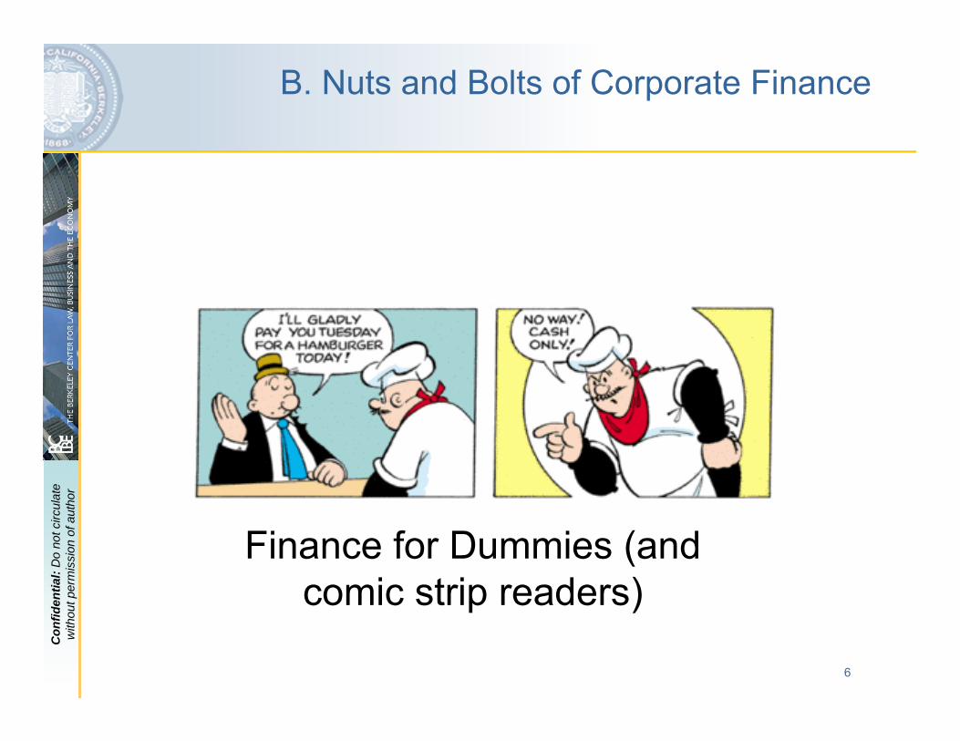
B. Nuts and Bolts of Corporate Finance
Finance for Dummies (and comic strip readers)
7
Con
fiden
tial:
Do
not c
ircul
ate
with
out p
erm
issi
on o
f aut
hor
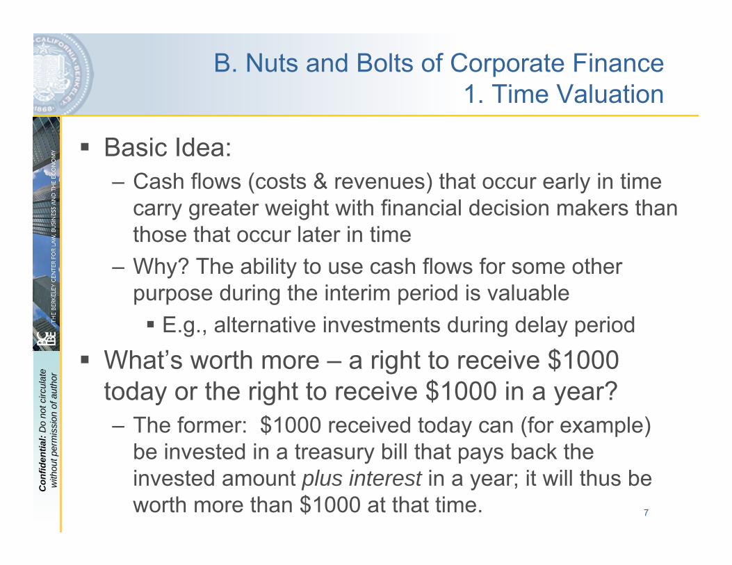
B. Nuts and Bolts of Corporate Finance 1. Time Valuation
Basic Idea:– Cash flows (costs & revenues) that occur early in time
carry greater weight with financial decision makers than those that occur later in time
– Why? The ability to use cash flows for some other purpose during the interim period is valuable
E.g., alternative investments during delay periodWhat’s worth more – a right to receive $1000 today or the right to receive $1000 in a year?– The former: $1000 received today can (for example)
be invested in a treasury bill that pays back the invested amount plus interest in a year; it will thus be worth more than $1000 at that time.

8
Con
fiden
tial:
Do
not c
ircul
ate
with
out p
erm
issi
on o
f aut
hor
Some (unavoidable) Notation
t = time (today is frequently denoted as “t=0”)T = terminal or “end” period (sometime in future)Ct = cash flow at time t
– Alternatively denoted as Ft or Pt (depending on use)r = “rate of return” from two periods of time
Most financial economists speak the language of returns– One Period Return (between t=0 and t=1):
– Multi-period Return (between t=0 and future date t)
r0,1 P 1 − P 0P 0
P 1P 0− 1
r0,t Pt − P 0
P 0 Pt
P 0− 1
9
Con
fiden
tial:
Do
not c
ircul
ate
with
out p
erm
issi
on o
f aut
hor
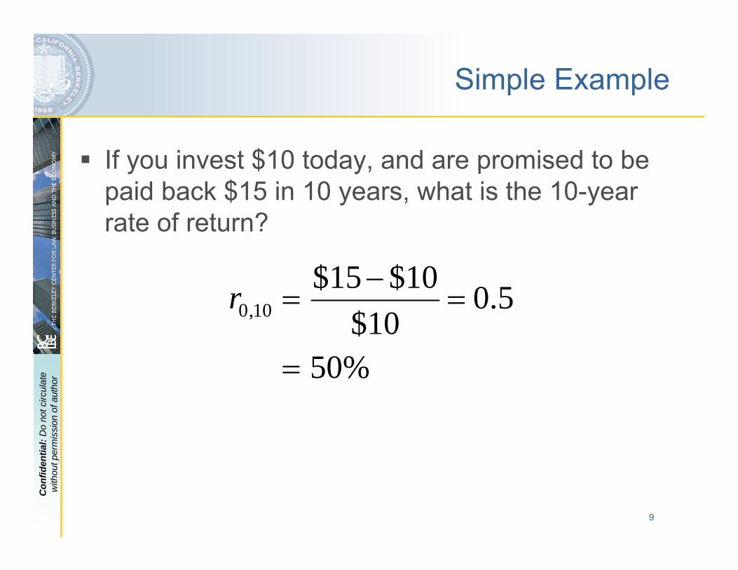
Simple Example
If you invest $10 today, and are promised to be paid back $15 in 10 years, what is the 10-year rate of return?
%50
5.010$
10$15$10,0
=
=−
=r
10
Con
fiden
tial:
Do
not c
ircul
ate
with
out p
erm
issi
on o
f aut
hor
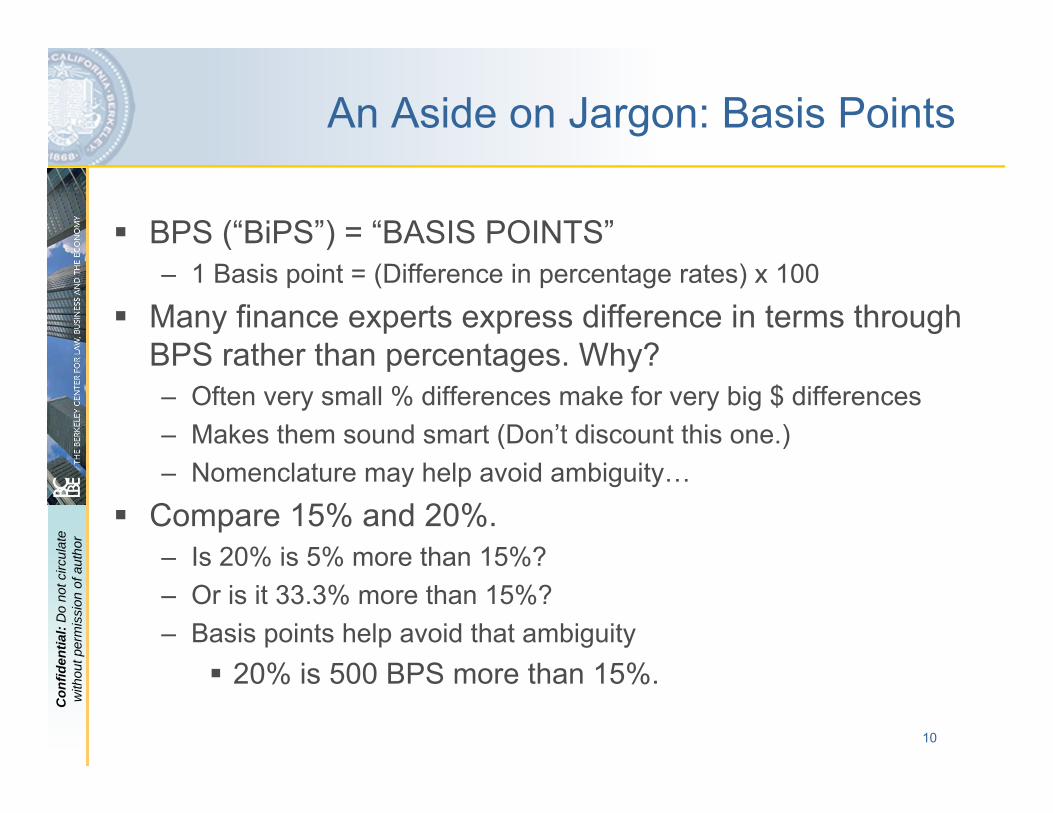
An Aside on Jargon: Basis Points
BPS (“BiPS”) = “BASIS POINTS”– 1 Basis point = (Difference in percentage rates) x 100
Many finance experts express difference in terms through BPS rather than percentages. Why?– Often very small % differences make for very big $ differences– Makes them sound smart (Don’t discount this one.)– Nomenclature may help avoid ambiguity…
Compare 15% and 20%.– Is 20% is 5% more than 15%?– Or is it 33.3% more than 15%?– Basis points help avoid that ambiguity
20% is 500 BPS more than 15%.

11
Con
fiden
tial:
Do
not c
ircul
ate
with
out p
erm
issi
on o
f aut
hor
Discounting and Compounding: (Get ready for a few formulas)
Functional Descriptions:– Compounding: How much will $X invested today be
worth in T years?– Discounting: How much is a future payment of $X
realized in T years worth today?The Baseline Formula(s)– Compounding: For a one-period investment of P
dollars at rate r, its future value F will be equal to:
– Discounting: The investment P necessary today at rate r to generate F dollars in the future will be equal to:
( )1,01 rPF +×=
)1( 1,0rFP
+=
KeyPointKeyPoint

12
Con
fiden
tial:
Do
not c
ircul
ate
with
out p
erm
issi
on o
f aut
hor
Compounding Over Multiple Periods
Compound interest over many (e.g., 20) Periods
In most contexts (though not all), the rate of return remains constant over time (at “r”). In this case, future value becomes:
F 20
F 20
F 2
F 1
P 0 1 r 0,1 1 r 1,2 . . .1 r 19,20
F 20 P 0
20 times
1 r 1 r . . .1 r
P 0 1 r20

14
Con
fiden
tial:
Do
not c
ircul
ate
with
out p
erm
issi
on o
f aut
hor
Compounding & Discounting when return is expected to remain constant
Compounding (from last slide):
Discounting to “Net Present Value” (for each future cash payment):
Discounting a “stream” of cash flows:
( )tr+1tF
( )tt rPF +×= 10
0P =
( ) ( ) ( )TT
rF
rF
rFFNPVP
+++
++
++==
1...
11 22
11
00
15
Con
fiden
tial:
Do
not c
ircul
ate
with
out p
erm
issi
on o
f aut
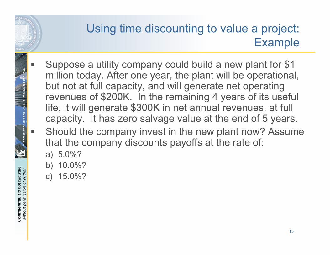
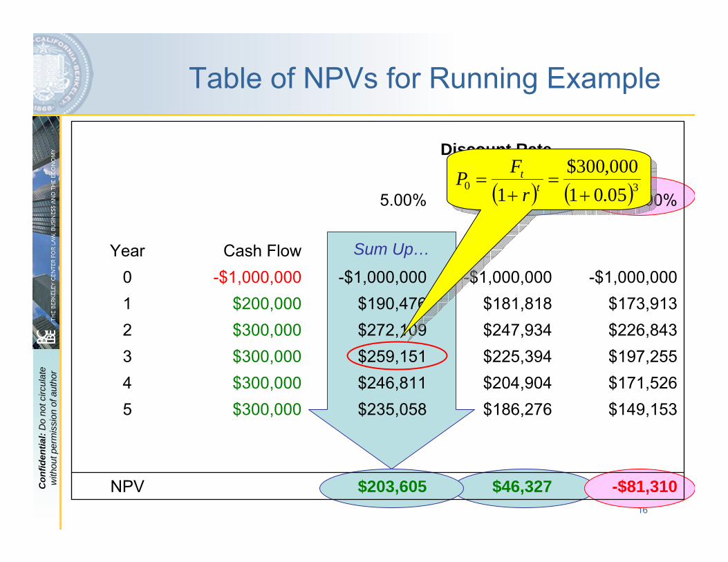
horUsing time discounting to value a project:
Example
Suppose a utility company could build a new plant for $1 million today. After one year, the plant will be operational, but not at full capacity, and will generate net operating revenues of $200K. In the remaining 4 years of its useful life, it will generate $300K in net annual revenues, at full capacity. It has zero salvage value at the end of 5 years.Should the company invest in the new plant now? Assume that the company discounts payoffs at the rate of:a) 5.0%?b) 10.0%?c) 15.0%?
16
Con
fiden
tial:
Do
not c
ircul
ate
with
out p
erm
issi
on o
f aut
hor
Sum Up…
-$81,310$46,327$203,605NPV
$149,153$186,276$235,058$300,0005$171,526$204,904$246,811$300,0004$197,255$225,394$259,151$300,0003$226,843$247,934$272,109$300,0002$173,913$181,818$190,476$200,0001
-$1,000,000-$1,000,000-$1,000,000-$1,000,0000Cash FlowYear
15.00%10.00%5.00%
Discount Rate
Table of NPVs for Running Example
( ) ( )30 05.01000,300$
1 +=
+= t
t
rFP
17
Con
fiden
tial:
Do
not c
ircul
ate
with
out p
erm
issi
on o
f aut
hor
Running Example (continued)
Suppose a utility company could build a new plant for $1 million today. After one year, the plant will be operational, but not at full capacity, and will generate net sales revenues of $200K. In the remaining 4 years of its useful life, it will generate $300K in net annual revenues, at full capacity. It has zero salvage value at the end of 5 years.Should the company invest in the new plant now? Assume that the company discounts payoffs at the risk-free rate:a) 5.0%?b) 10.0%?c) 15.0%?Suppose the utility invests in the above project, and the project is its only activity. Suppose that the utility is publicly traded, has no debt, and pays all its net revenues out as dividends each year. Its 100,000 shares are currently trading for $1 each. At what rate of return do investors appear to discount the utility’s market value?
18
Con
fiden
tial:
Do
not c
ircul
ate
with
out p
erm
issi
on o
f aut
hor
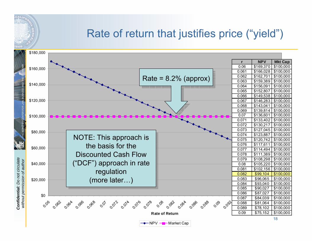
Rate of return that justifies price (“yield”)
$0
$20,000
$40,000
$60,000
$80,000
$100,000
$120,000
$140,000
$160,000
$180,000
0.06
0.062
0.064
0.066
0.068
0.07
0.072
0.074
0.076
0.078
0.080.08
20.0
840.0
860.0
88 0.09
0.092
0.094
0.096
0.098 0.1
Rate of Return
NP
V
NPV Market Cap
Rate = 8.2% (approx)Rate = 8.2% (approx)
NOTE: This approach is the basis for the
Discounted Cash Flow (“DCF”) approach in rate
regulation (more later…)
NOTE: This approach is the basis for the
Discounted Cash Flow (“DCF”) approach in rate
regulation (more later…)
r NPV Mkt Cap0.06 $169,370 $100,0000.061 $166,028 $100,0000.062 $162,701 $100,0000.063 $159,389 $100,0000.064 $156,091 $100,0000.065 $152,807 $100,0000.066 $149,538 $100,0000.067 $146,283 $100,0000.068 $143,041 $100,0000.069 $139,814 $100,0000.07 $136,601 $100,0000.071 $133,402 $100,0000.072 $130,217 $100,0000.073 $127,045 $100,0000.074 $123,887 $100,0000.075 $120,742 $100,0000.076 $117,611 $100,0000.077 $114,494 $100,0000.078 $111,389 $100,0000.079 $108,298 $100,0000.08 $105,220 $100,0000.081 $102,156 $100,0000.082 $99,104 $100,0000.083 $96,065 $100,0000.084 $93,040 $100,0000.085 $90,027 $100,0000.086 $87,027 $100,0000.087 $84,039 $100,0000.088 $81,064 $100,0000.089 $78,102 $100,0000.09 $75,152 $100,000

19
Con
fiden
tial:
Do
not c
ircul
ate
with
out p
erm
issi
on o
f aut
hor
Discounting when rate of return (r) is constant and cash flows (F) have consistent pattern
Constant stream of cash flows (annuity of $F / period):
Note: as T grows arbitrarily large (perpetuity of $F/period):
Constantly growing stream of cash flows (at rate g)
As T grows arbitrarily large (and assuming g<r):
rFNPV =
( ) ( ) ( ) ⎟⎟⎠
⎞⎜⎜⎝
⎛+
−×=+
+++
++
= TT rrF
rF
rF
rFNPV
)1(11
1...
11 21
( )( )
( )( )( ) ⎟⎟
⎠
⎞⎜⎜⎝
⎛++
−×−
=++
++++
++
=−
T
T
T
T
rg
grF
rgF
rgF
rFNPV
)1()1(1
11...
11
1
1
2
1
1
grFNPV−
= Commonly used in DCF valuation analyses (Gordon Div. Growth Model); see below.
Commonly used in DCF valuation analyses (Gordon Div. Growth Model); see below.

20
Con
fiden
tial:
Do
not c
ircul
ate
with
out p
erm
issi
on o
f aut
hor
Rules of Thumb from Time Valuation
Most investors / financial decision makers will make an investment only when the Net Present Value (NPV) of the project is positive.Holding all else constant, the NPV of a “typical”investment’s cash flow pattern increases when…
1. …up-front costs decrease2. …the size of follow-on benefits increases3. …the period over which follow-on benefits accrue increases4. …the rate at which market actors discount the future decreases
Economic factors / policies that bring about (1) – (4) tend to increase investment.
And, vice versa, things that reverse (1) – (4) tend to discourage investment.
KeyPointKeyPoint
21
Con
fiden
tial:
Do
not c
ircul
ate
with
out p
erm
issi
on o
f aut
hor
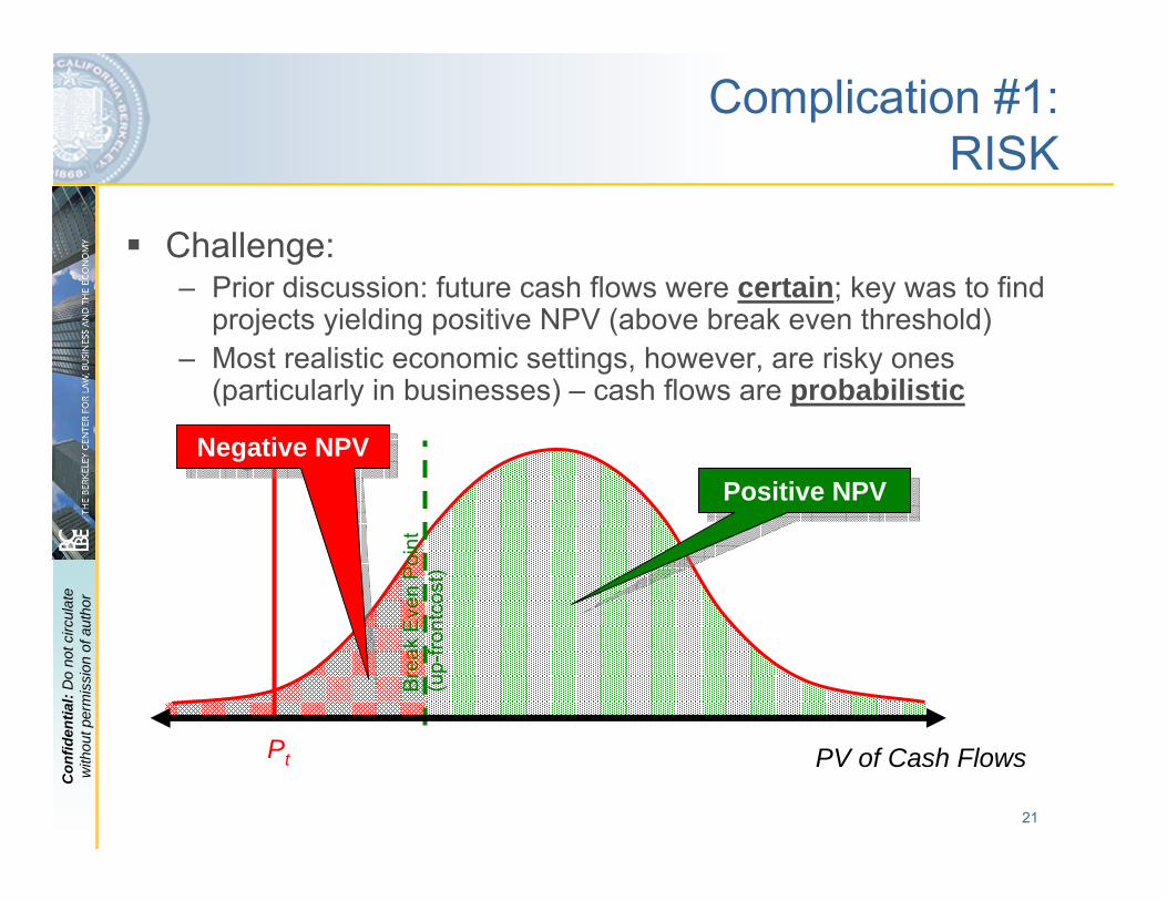
Complication #1:RISK
Challenge:– Prior discussion: future cash flows were certain; key was to find
projects yielding positive NPV (above break even threshold)– Most realistic economic settings, however, are risky ones
(particularly in businesses) – cash flows are probabilistic
Pt
Bre
ak E
ven
Poi
nt
(up-
front
cost
)
PV of Cash Flows
Positive NPVPositive NPVNegative NPVNegative NPV

22
Con
fiden
tial:
Do
not c
ircul
ate
with
out p
erm
issi
on o
f aut
hor
Complication #2: CAPITAL STRUCTURE
Many utilities have multiple classes of investors, each with different claims on cash flowsConventional/simple distinction:– Debt/Bonds: “Fixed” claim; priority
(first dibs) on revenues– Equity/Stock: “Residual” claim;
back seat on claims to revenuesConsequences of capital structure (+ risk) for finance:– For a given pattern of risky cash
flows, debt is safer than equity. – Expected/required return on debt
(ROD) is lower than expected return on equity (ROE)
– ROD, ROE, and Δ=(ROE-ROD) all tend to increase in leverage(though total cost of capital could go up or down)
Rev
enue
sR
even
ues
Debt
Equity

23
Con
fiden
tial:
Do
not c
ircul
ate
with
out p
erm
issi
on o
f aut
hor
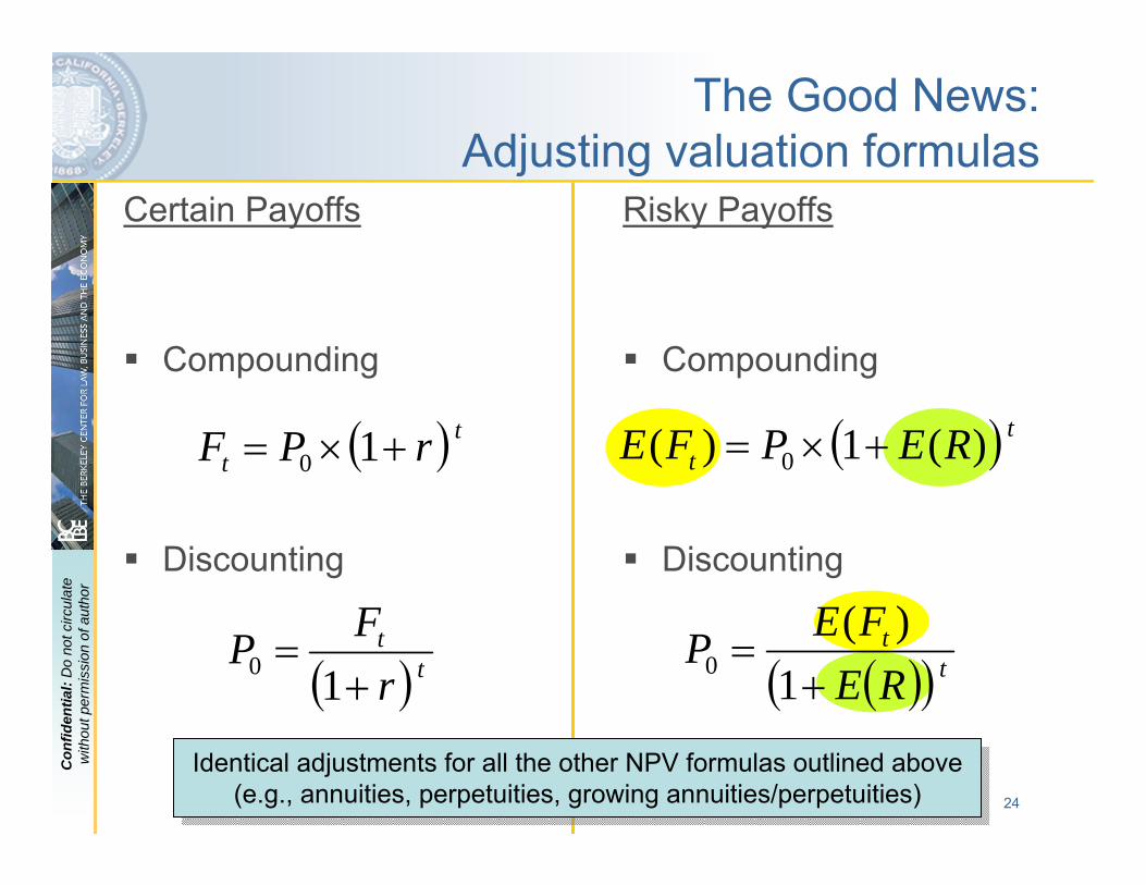
Adjusting valuation analysis to account for the risky environments
The Good News:– Most of the rules of thumb about time discounting /
compounding still hold– In fact, all of the FV / PV expressions above still apply,
in very much the same forms before…
The Bad News:– Applying of these formulas can be a bit more complex,
in at least three ways. We now must focus on:Expected cash flows (e.g., cash flows “on average”); Risk-Adjusted Expected rates of return;Combining Expected Returns Different Classes of Investors (e.g., ROD & ROE) using the “WACC”
24
Con
fiden
tial:
Do
not c
ircul
ate
with
out p
erm
issi
on o
f aut
hor
The Good News:Adjusting valuation formulas
Certain Payoffs
Compounding
Discounting
Risky Payoffs
Compounding
Discounting
( ) tt REPFE
0 )(1)( +×=
( ) tt
rFP 0 1+
=
( ) tt rPF
0 1+×=
( )( ) tt
REFEP 0 1
)(+
=
Identical adjustments for all the other NPV formulas outlined above (e.g., annuities, perpetuities, growing annuities/perpetuities)
Identical adjustments for all the other NPV formulas outlined above (e.g., annuities, perpetuities, growing annuities/perpetuities)
25
Con
fiden
tial:
Do
not c
ircul
ate
with
out p
erm
issi
on o
f aut
hor
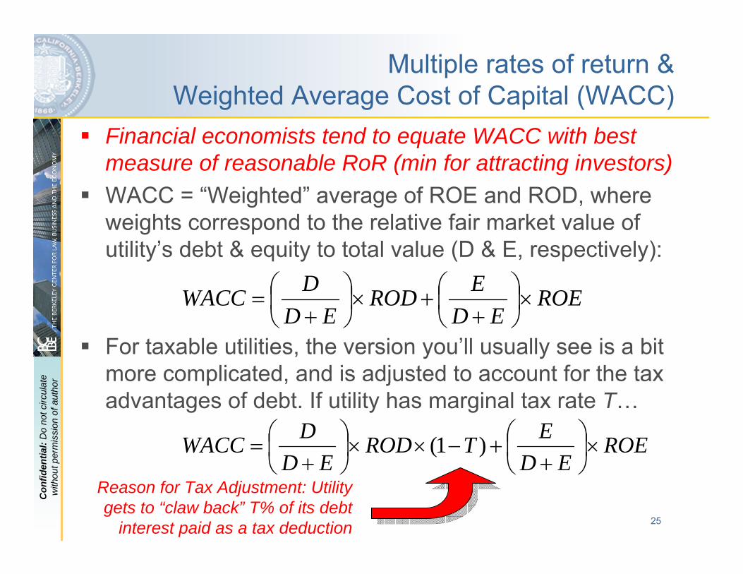
Multiple rates of return &Weighted Average Cost of Capital (WACC)
Financial economists tend to equate WACC with best measure of reasonable RoR (min for attracting investors)WACC = “Weighted” average of ROE and ROD, where weights correspond to the relative fair market value of utility’s debt & equity to total value (D & E, respectively):
For taxable utilities, the version you’ll usually see is a bit more complicated, and is adjusted to account for the tax advantages of debt. If utility has marginal tax rate T…
ROEED
ERODED
DWACC ×⎟⎠⎞
⎜⎝⎛
++×⎟
⎠⎞
⎜⎝⎛
+=
ROEED
ETRODED
DWACC ×⎟⎠⎞
⎜⎝⎛
++−××⎟
⎠⎞
⎜⎝⎛
+= )1(
Reason for Tax Adjustment: Utility gets to “claw back” T% of its debt
interest paid as a tax deduction

26
Con
fiden
tial:
Do
not c
ircul
ate
with
out p
erm
issi
on o
f aut
hor
Estimating WACC requires an estimating expected returns of capital claims (ROE; ROD)
Investors don’t know what their actual realized return will be on their investment.Instead, they forecast an expected return:– Effectively, what return they expect to receive on
average from holding the investment across periods– They then can use those expected returns to discount
future cash flow payments.2 dominant ways to estimate expected ROE/ROD:– Discounted Cash Flow (DCF) approach– Capital Asset Pricing Model (CAPM) approach– Often valuation experts use both approaches
27
Con
fiden
tial:
Do
not c
ircul
ate
with
out p
erm
issi
on o
f aut
hor
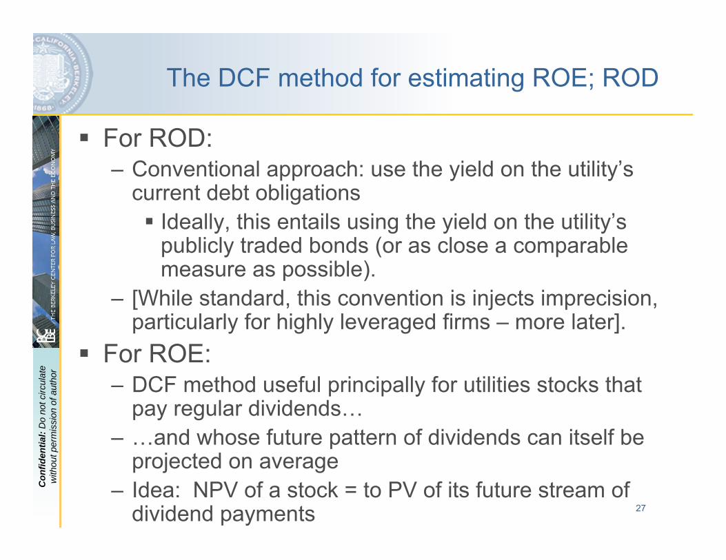
The DCF method for estimating ROE; ROD
For ROD:– Conventional approach: use the yield on the utility’s
current debt obligationsIdeally, this entails using the yield on the utility’s publicly traded bonds (or as close a comparable measure as possible).
– [While standard, this convention is injects imprecision, particularly for highly leveraged firms – more later].
For ROE:– DCF method useful principally for utilities stocks that
pay regular dividends…– …and whose future pattern of dividends can itself be
projected on average– Idea: NPV of a stock = to PV of its future stream of
dividend payments
28
Con
fiden
tial:
Do
not c
ircul
ate
with
out p
erm
issi
on o
f aut
hor
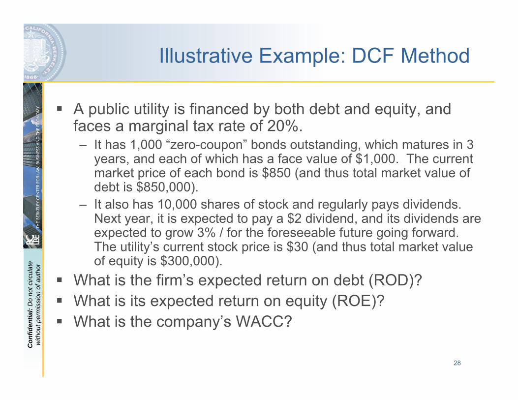
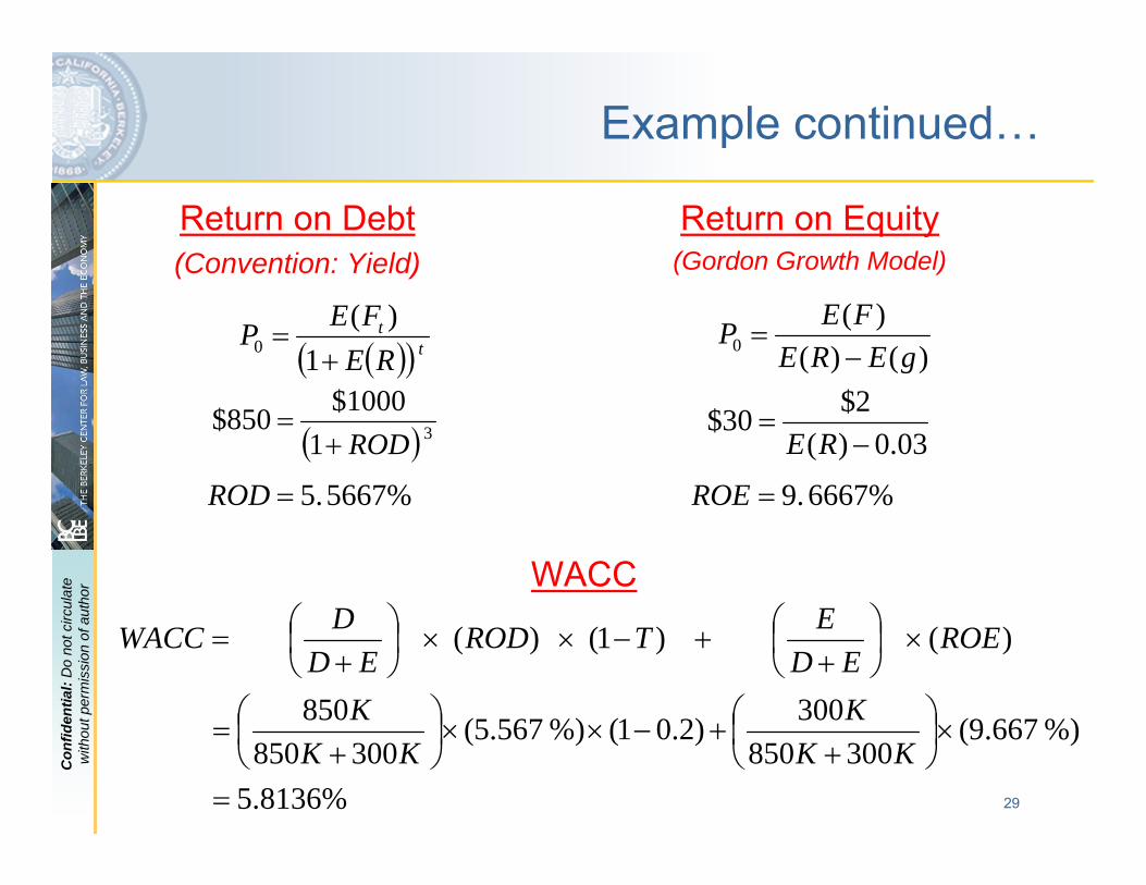
Illustrative Example: DCF Method
A public utility is financed by both debt and equity, and faces a marginal tax rate of 20%.– It has 1,000 “zero-coupon” bonds outstanding, which matures in 3
years, and each of which has a face value of $1,000. The current market price of each bond is $850 (and thus total market value of debt is $850,000).
– It also has 10,000 shares of stock and regularly pays dividends.Next year, it is expected to pay a $2 dividend, and its dividends are expected to grow 3% / for the foreseeable future going forward. The utility’s current stock price is $30 (and thus total market value of equity is $300,000).
What is the firm’s expected return on debt (ROD)? What is its expected return on equity (ROE)?What is the company’s WACC?
29
Con
fiden
tial:
Do
not c
ircul
ate
with
out p
erm
issi
on o
f aut
hor
Example continued…
Return on Debt(Convention: Yield)
( )( ) tt
REFEP 0 1
)(+
=
( ) 3 11000$850$ROD+
=
5667% 5.=ROD
)()()(
0 gEREFEP
−=
6667% 9.=ROE
03.0)(2$30$−
=RE
Return on Equity(Gordon Growth Model)
5.8136%
%) 667.9(300850
300)2.01(%) 567.5(300850
850
)( )1( )(
=
×⎟⎠⎞
⎜⎝⎛
++−××⎟
⎠⎞
⎜⎝⎛
+=
×⎟⎠⎞
⎜⎝⎛
++−××⎟
⎠⎞
⎜⎝⎛
+=
KKK
KKK
ROEED
ETRODED
DWACC
WACC
30
Con
fiden
tial:
Do
not c
ircul
ate
with
out p
erm
issi
on o
f aut
hor
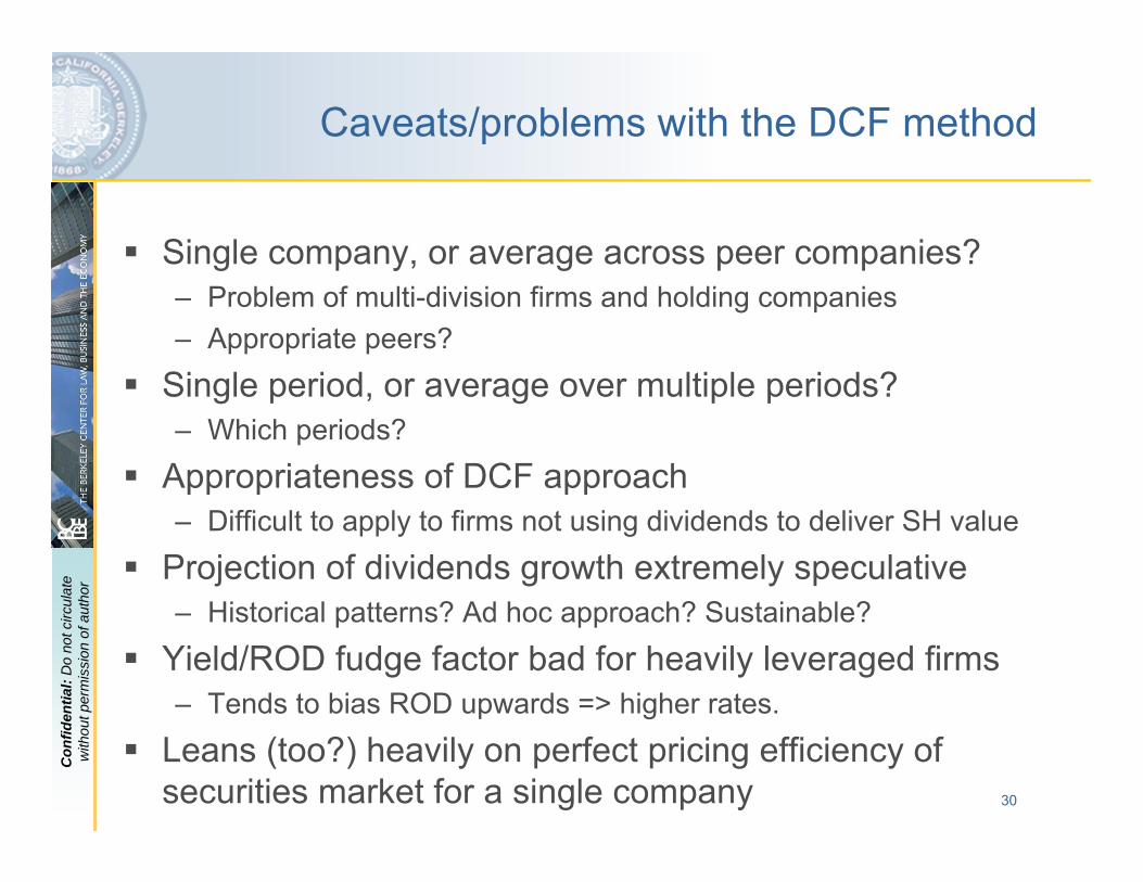
Caveats/problems with the DCF method
Single company, or average across peer companies?– Problem of multi-division firms and holding companies– Appropriate peers?
Single period, or average over multiple periods?– Which periods?
Appropriateness of DCF approach – Difficult to apply to firms not using dividends to deliver SH value
Projection of dividends growth extremely speculative– Historical patterns? Ad hoc approach? Sustainable?
Yield/ROD fudge factor bad for heavily leveraged firms– Tends to bias ROD upwards => higher rates.
Leans (too?) heavily on perfect pricing efficiency of securities market for a single company
31
Con
fiden
tial:
Do
not c
ircul
ate
with
out p
erm
issi
on o
f aut
hor
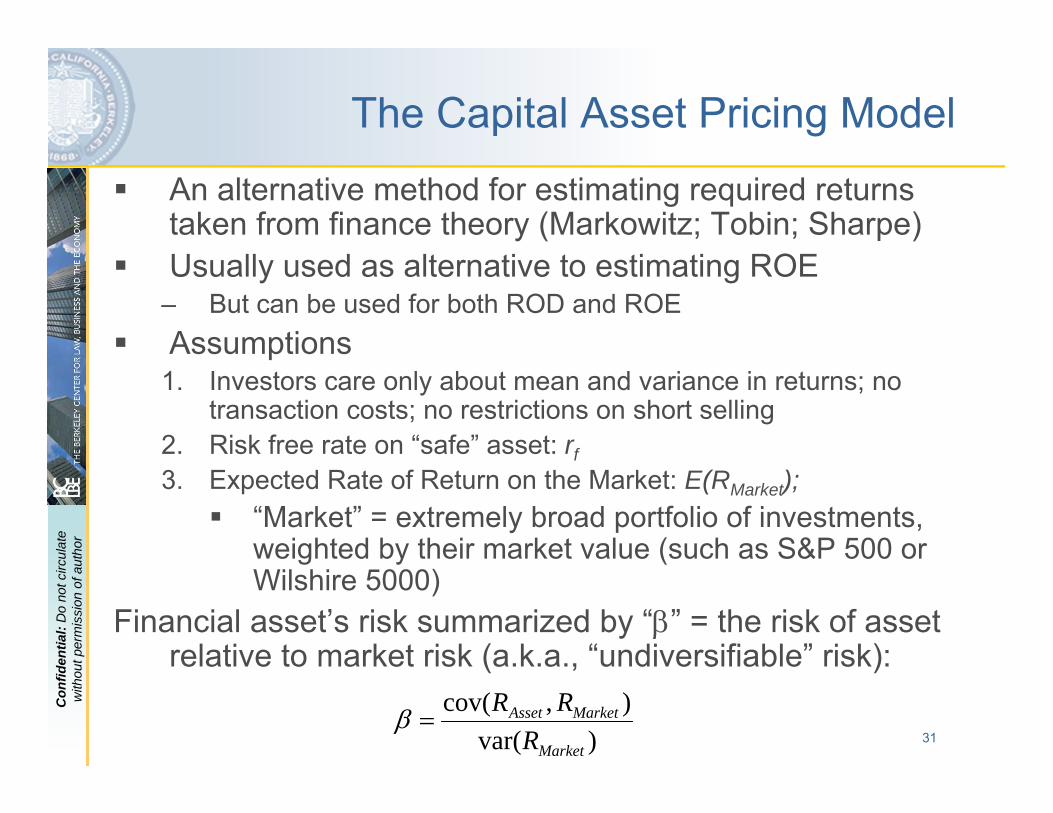
The Capital Asset Pricing Model
An alternative method for estimating required returns taken from finance theory (Markowitz; Tobin; Sharpe)Usually used as alternative to estimating ROE
– But can be used for both ROD and ROEAssumptions
1. Investors care only about mean and variance in returns; no transaction costs; no restrictions on short selling
2. Risk free rate on “safe” asset: rf3. Expected Rate of Return on the Market: E(RMarket);
“Market” = extremely broad portfolio of investments, weighted by their market value (such as S&P 500 or Wilshire 5000)
Financial asset’s risk summarized by “β” = the risk of asset relative to market risk (a.k.a., “undiversifiable” risk):
)var(),cov(
Market
MarketAsset
RRR
=β
32
Con
fiden
tial:
Do
not c
ircul
ate
with
out p
erm
issi
on o
f aut
hor
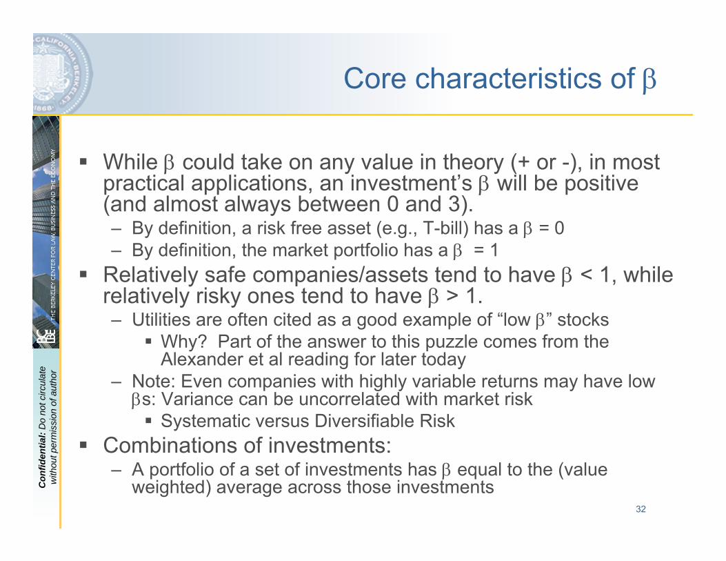
Core characteristics of β
While β could take on any value in theory (+ or -), in most practical applications, an investment’s β will be positive (and almost always between 0 and 3).– By definition, a risk free asset (e.g., T-bill) has a β = 0– By definition, the market portfolio has a β = 1
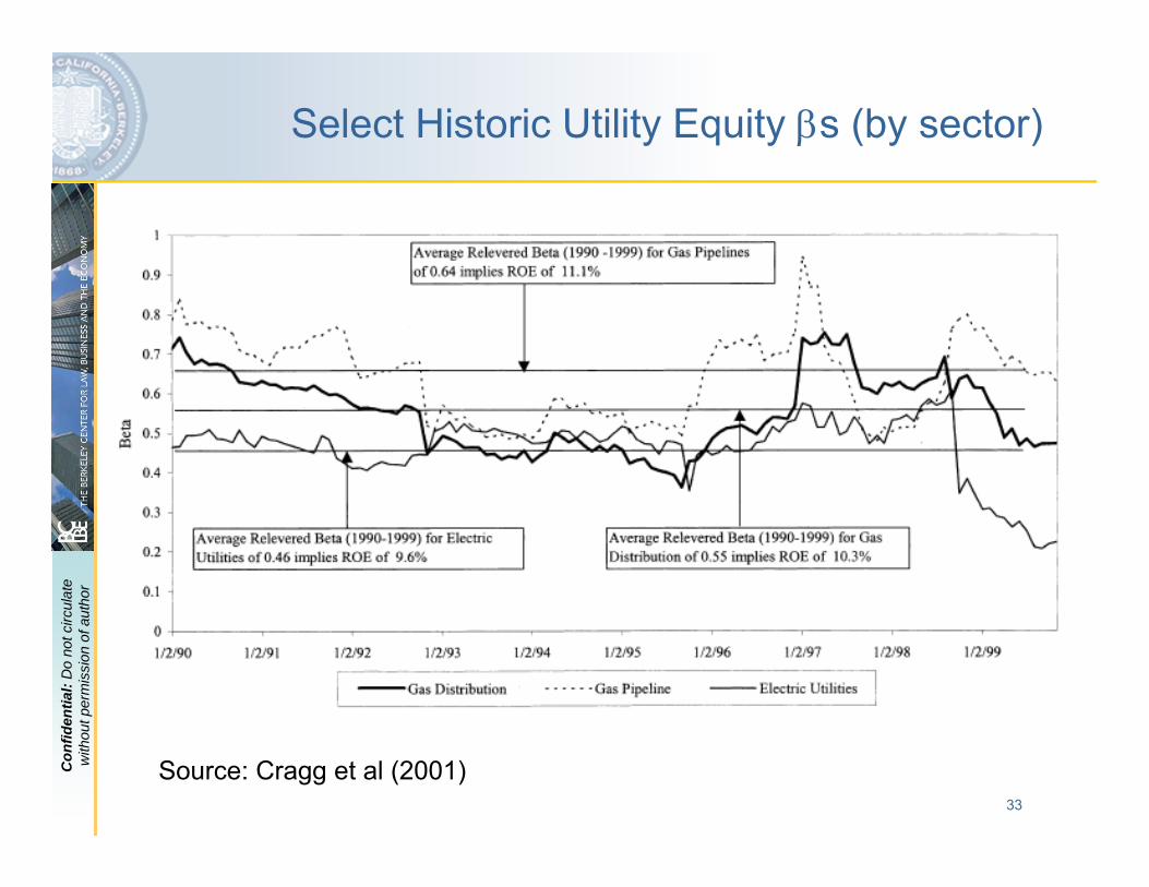
Relatively safe companies/assets tend to have β < 1, while relatively risky ones tend to have β > 1.– Utilities are often cited as a good example of “low β” stocks
Why? Part of the answer to this puzzle comes from the Alexander et al reading for later today
– Note: Even companies with highly variable returns may have low βs: Variance can be uncorrelated with market risk
Systematic versus Diversifiable RiskCombinations of investments:– A portfolio of a set of investments has β equal to the (value
weighted) average across those investments
33
Con
fiden
tial:
Do
not c
ircul
ate
with
out p
erm
issi
on o
f aut
hor
Select Historic Utility Equity βs (by sector)
Source: Cragg et al (2001)

34
Con
fiden
tial:
Do
not c
ircul
ate
with
out p
erm
issi
on o
f aut
hor
β
Retu
rn
Using β to estimate expected return: The CAPM Securities Market Line
( )fMktfA rRErRE −×+= )()( β
E(RMkt)
β = 0 β = 1
rf
35
Con
fiden
tial:
Do
not c
ircul
ate
with
out p
erm
issi
on o
f aut
hor
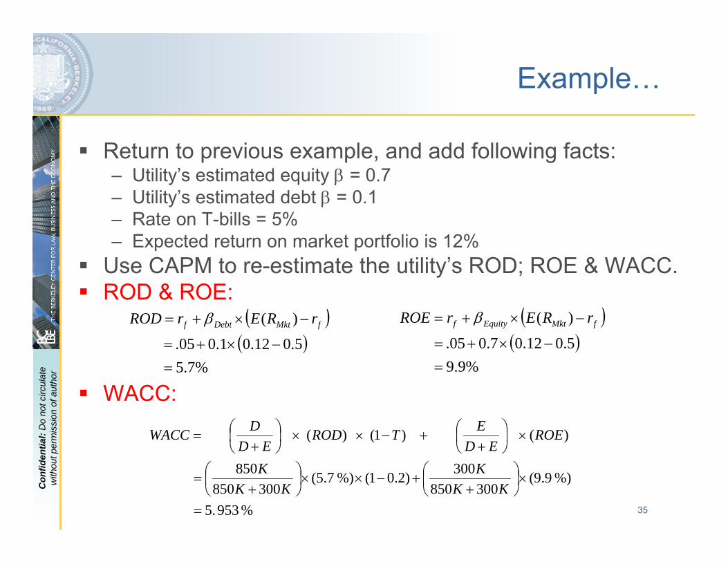
Example…
Return to previous example, and add following facts:– Utility’s estimated equity β = 0.7– Utility’s estimated debt β = 0.1– Rate on T-bills = 5%– Expected return on market portfolio is 12%
Use CAPM to re-estimate the utility’s ROD; ROE & WACC.ROD & ROE:
WACC:
% 953 5.
%) 9.9(300850
300)2.01(%) 7.5(300850
850
)( )1( )(
=
×⎟⎠⎞
⎜⎝⎛
++−××⎟
⎠⎞
⎜⎝⎛
+=
×⎟⎠⎞
⎜⎝⎛
++−××⎟
⎠⎞
⎜⎝⎛
+=
KKK
KKK
ROEED
ETRODED
DWACC
( )( )
%9.9 5.012.07.005.
)(
=−×+=
−×+= fMktEquityf rRErROE β( )( )
%7.5 5.012.01.005.
)(
=−×+=
−×+= fMktDebtf rRErROD β
36
Con
fiden
tial:
Do
not c
ircul
ate
with
out p
erm
issi
on o
f aut
hor
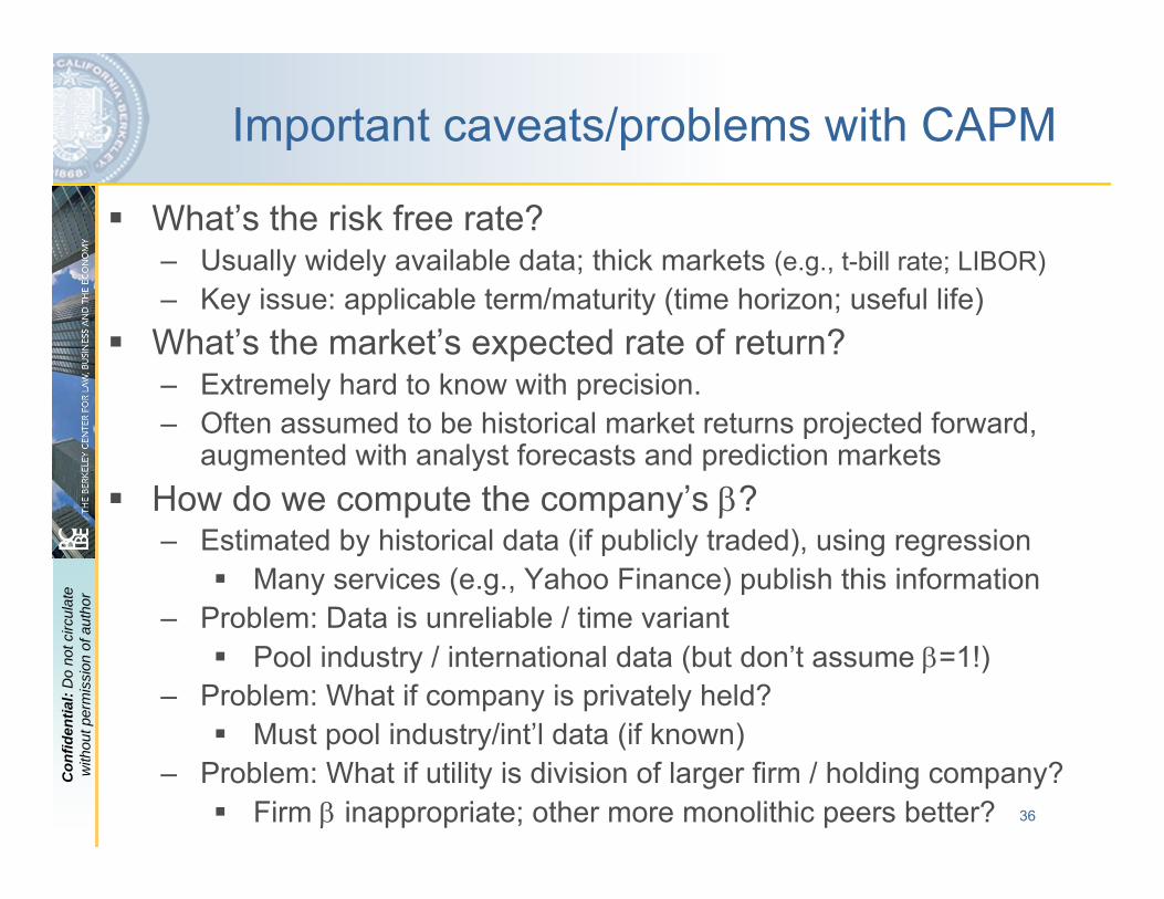
Important caveats/problems with CAPM
What’s the risk free rate?– Usually widely available data; thick markets (e.g., t-bill rate; LIBOR)– Key issue: applicable term/maturity (time horizon; useful life)What’s the market’s expected rate of return?– Extremely hard to know with precision. – Often assumed to be historical market returns projected forward,
augmented with analyst forecasts and prediction marketsHow do we compute the company’s β?– Estimated by historical data (if publicly traded), using regression
Many services (e.g., Yahoo Finance) publish this information– Problem: Data is unreliable / time variant
Pool industry / international data (but don’t assume β=1!)– Problem: What if company is privately held?
Must pool industry/int’l data (if known)– Problem: What if utility is division of larger firm / holding company?
Firm β inappropriate; other more monolithic peers better?
37
Con
fiden
tial:
Do
not c
ircul
ate
with
out p
erm
issi
on o
f aut
hor
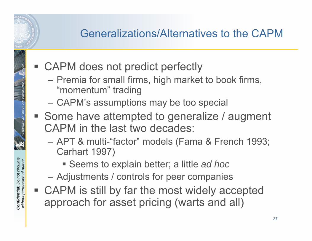
Generalizations/Alternatives to the CAPM
CAPM does not predict perfectly– Premia for small firms, high market to book firms,
“momentum” trading– CAPM’s assumptions may be too special
Some have attempted to generalize / augment CAPM in the last two decades:– APT & multi-“factor” models (Fama & French 1993;
Carhart 1997)Seems to explain better; a little ad hoc
– Adjustments / controls for peer companiesCAPM is still by far the most widely accepted approach for asset pricing (warts and all)

38
Con
fiden
tial:
Do
not c
ircul
ate
with
out p
erm
issi
on o
f aut
hor
Rules of Thumb from Risk ValuationFinancial decision makers make risky investment choices according the NPV rule adjusted for risk.Holding all else constant, the risk-adjusted NPV of a typical investment’s cash flow pattern increases when…
1. …up-front costs decline2. …the expected size of downstream benefits increases3. …the period over which downstream benefits accrue lengthens4. …the risk free rate of return decreases5. …the expected market rate of return decreases6. …the company’s market β decreases
Economic factors / policies that bring about (1) – (6) tend to catalyze investment.
And, vice versa, things that reverse (1) – (6) tend to decrease investment.
KeyPointKeyPoint
39
Con
fiden
tial:
Do
not c
ircul
ate
with
out p
erm
issi
on o
f aut
hor
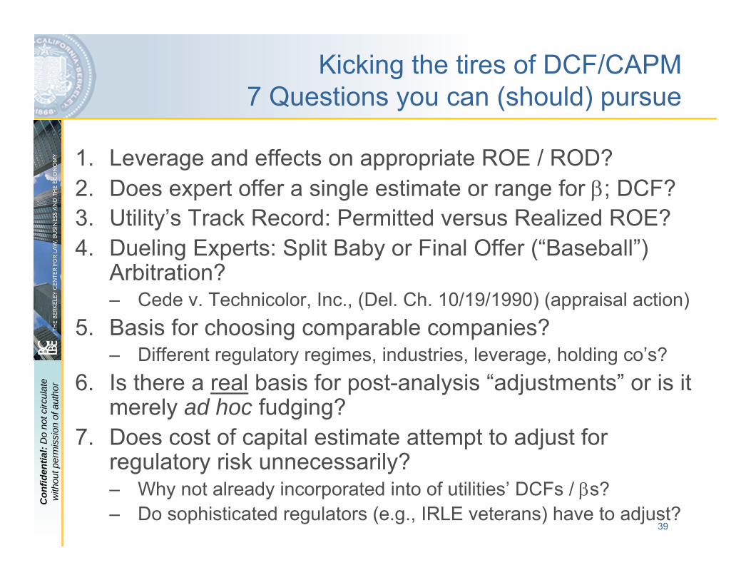
Kicking the tires of DCF/CAPM7 Questions you can (should) pursue
1. Leverage and effects on appropriate ROE / ROD?2. Does expert offer a single estimate or range for β; DCF?3. Utility’s Track Record: Permitted versus Realized ROE?4. Dueling Experts: Split Baby or Final Offer (“Baseball”)
Arbitration?– Cede v. Technicolor, Inc., (Del. Ch. 10/19/1990) (appraisal action)
5. Basis for choosing comparable companies?– Different regulatory regimes, industries, leverage, holding co’s?
6. Is there a real basis for post-analysis “adjustments” or is it merely ad hoc fudging?
7. Does cost of capital estimate attempt to adjust for regulatory risk unnecessarily?– Why not already incorporated into of utilities’ DCFs / βs?– Do sophisticated regulators (e.g., IRLE veterans) have to adjust?

40
Con
fiden
tial:
Do
not c
ircul
ate
with
out p
erm
issi
on o
f aut
hor
3. Regulatory Risk
Regulated companies ≠ non-profits. – Just like other for-profit firms, they make decisions that are in their
investors’ long-term financial interests– Thus, such companies still make investment / operational
decisions that are predicated on maximizing risk-adjusted present value to investors
The Big Difference: Regulatory Risk– In addition to market conditions, costs, rate fluctuations, etc, the
regulator’s actions (and future anticipated actions) bear on the nature, timing, magnitude, and sustainability of future cash flows
– Moreover, and somewhat troublingly, cash flow patterns of the regulated company can bear on the regulator’s actions…
…which can in turn affect the company’s cash flow patterns……which can in turn affect the regulator’s actions……etc…
41
Con
fiden
tial:
Do
not c
ircul
ate
with
out p
erm
issi
on o
f aut
hor
C. The multiple faces of regulatory risk
RR as a type of insurance
RR as a type of volatility
RR as a type of return truncation
Balancing commitment & flexibility

42
Con
fiden
tial:
Do
not c
ircul
ate
with
out p
erm
issi
on o
f aut
hor
Regulation as Insurance/Reduced Volatility
Textbook Rate of Return regulation = guaranteed return; perfect insurance against cost fluctuations– Perfect ROR reg. => reasonable rate = T-bill rate– Never true in practice (regulatory lag; private
information/gaming; incentives; other types of RR)Nevertheless, estimated βs for RoR regulated firms historically lower than for price cap firms– Incentives / investment tradeoff– Evidence is perhaps weaker than one might think
Here, anticipated regulatory safety nets may subsidize inefficient or excess investment

43
Con
fiden
tial:
Do
not c
ircul
ate
with
out p
erm
issi
on o
f aut
hor
Alexander et al (1996)
Punch-line?
More recent evidence is much weaker. Implications?

44
Con
fiden
tial:
Do
not c
ircul
ate
with
out p
erm
issi
on o
f aut
hor
Regulation as a source of added volatility
Unpredictability of regulation (even in RoRregimes) can enhance volatility utility’s returnsCan lead to lower expected cash flows and/or higher βs, with a higher required rate of return
Future Cash Flows
Bre
ak E
ven
Thre
shol
d
45
Con
fiden
tial:
Do
not c
ircul
ate
with
out p
erm
issi
on o
f aut
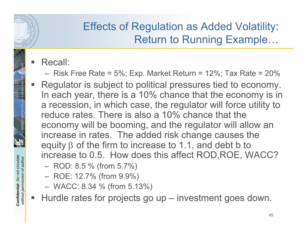
horEffects of Regulation as Added Volatility:
Return to Running Example…
Recall:– Risk Free Rate = 5%; Exp. Market Return = 12%; Tax Rate = 20%
Regulator is subject to political pressures tied to economy. In each year, there is a 10% chance that the economy is in a recession, in which case, the regulator will force utility to reduce rates. There is also a 10% chance that the economy will be booming, and the regulator will allow an increase in rates. The added risk change causes the equity β of the firm to increase to 1.1, and debt b to increase to 0.5. How does this affect ROD,ROE, WACC?– ROD: 8.5 % (from 5.7%)– ROE: 12.7% (from 9.9%)– WACC: 8.34 % (from 5.13%)
Hurdle rates for projects go up – investment goes down.
46
Con
fiden
tial:
Do
not c
ircul
ate
with
out p
erm
issi
on o
f aut
hor
Note…
Sometimes regulatory risk harbors cataclysmic forms of volatility– E.g., in many industries, doing business requires one to
be in good standing among regulatory authority– Ability to revoke / suspend licenses has significant
implicationsArthur Andersen (“Big 5” accounting firm)ITTGE Medical Systems
However, regulatory risk may also serve to moderate risks (see above)
47
Con
fiden
tial:
Do
not c
ircul
ate
with
out p
erm
issi
on o
f aut
hor
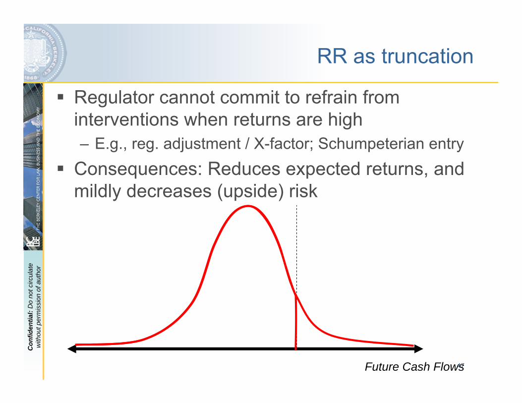
RR as truncation
Regulator cannot commit to refrain from interventions when returns are high– E.g., reg. adjustment / X-factor; Schumpeterian entry
Consequences: Reduces expected returns, and mildly decreases (upside) risk
Future Cash Flows
48
Con
fiden
tial:
Do
not c
ircul
ate
with
out p
erm
issi
on o
f aut
hor
How to deal with these issues?
Most commonly proposed way to address:– Regulatory Commitment
But commitment depends on numerous factors– Sufficient information to “get it right” ex ante– Legal/constitutional constraints (binding successors)– Value of flexibility to adapt to changing conditions– Regulatory structure that is self-correcting
Potential advantage of RoR regulation?– Political Cycles
Possibly easier to strike deals right after electoral cycle

49
Con
fiden
tial:
Do
not c
ircul
ate
with
out p
erm
issi
on o
f aut
hor
3. Valuing Options
Motivation:– The logic of NPV has thus far served us well;– But it sometimes happens that even relatively attractive projects
with positive NPV (underinvestment in technology in established generation networks)
– This lack of interest sometimes leaves people scratching their heads. Unobservable risk? Irrationality? Gamesmanship?
– Perhaps: However, it may also be because the potential investor is not only deciding whether to invest, but is also deciding about when to make the decision
Real Option:– The existence of an ability to alter strategies / decisions in order
adapt to new information, in order to make more profitable decisions or avoid losses
50
Con
fiden
tial:
Do
not c
ircul
ate
with
out p
erm
issi
on o
f aut
hor
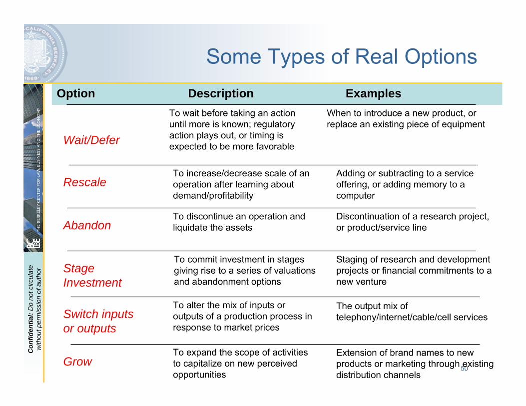
Wait/Defer
Rescale
Abandon
Switch inputs or outputs
Grow
To wait before taking an action until more is known; regulatory action plays out, or timing is expected to be more favorable
To increase/decrease scale of an operation after learning about demand/profitability
To discontinue an operation and liquidate the assets
To commit investment in stages giving rise to a series of valuations and abandonment options
To alter the mix of inputs or outputs of a production process in response to market prices
Stage Investment
To expand the scope of activities to capitalize on new perceived opportunities
ExamplesDescriptionOption
Adding or subtracting to a service offering, or adding memory to a computer
When to introduce a new product, or replace an existing piece of equipment
Discontinuation of a research project, or product/service line
Staging of research and development projects or financial commitments to a new venture
The output mix of telephony/internet/cable/cell services
Extension of brand names to new products or marketing through existing distribution channels
Some Types of Real Options
51
Con
fiden
tial:
Do
not c
ircul
ate
with
out p
erm
issi
on o
f aut
hor
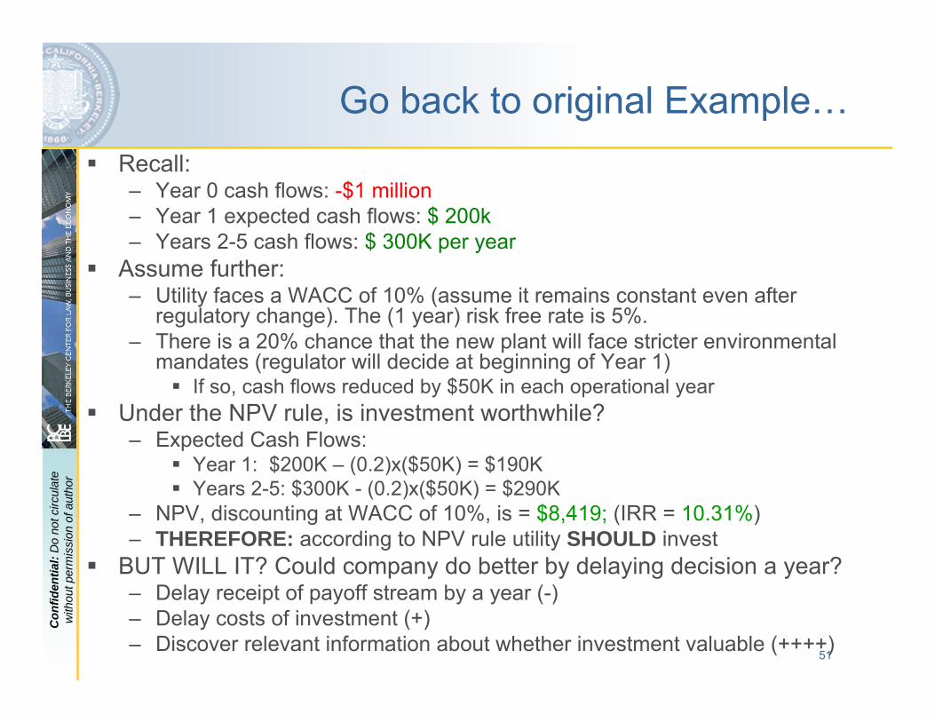
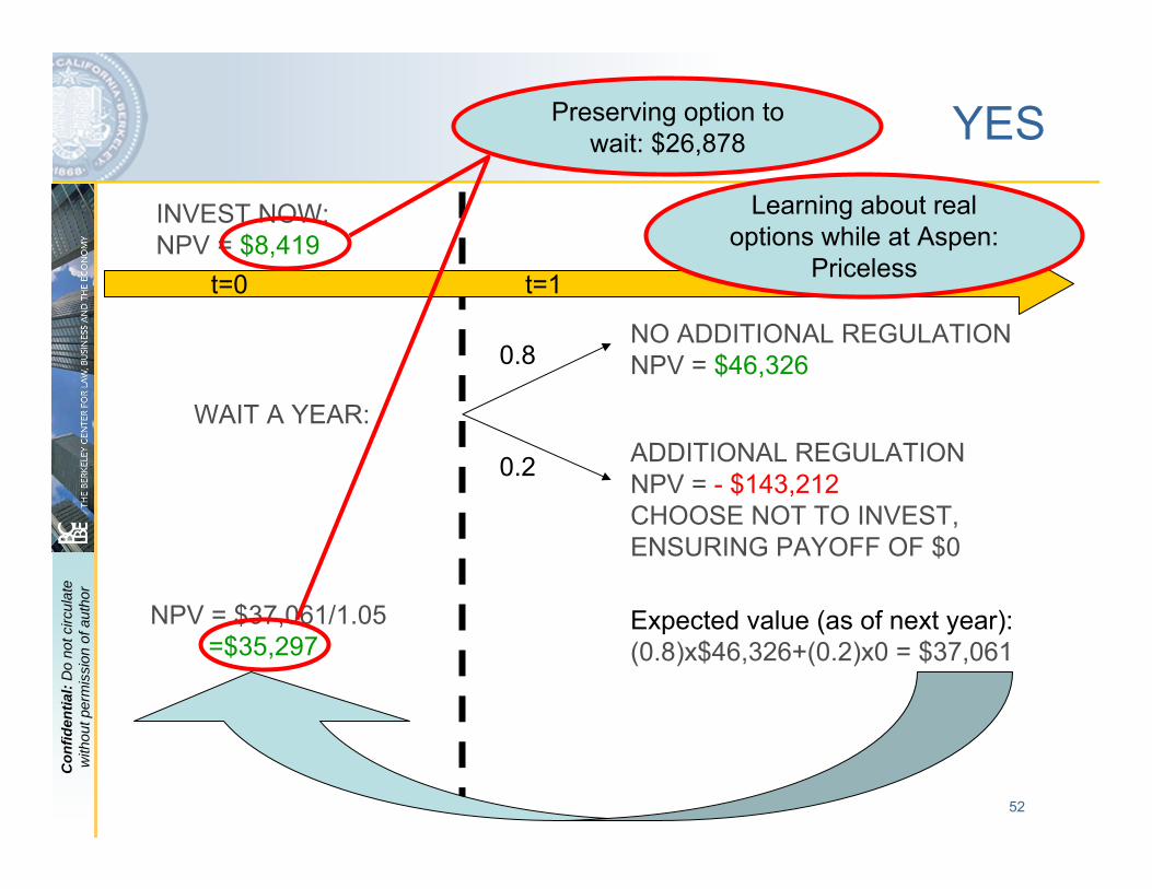
Go back to original Example…Recall:– Year 0 cash flows: -$1 million– Year 1 expected cash flows: $ 200k– Years 2-5 cash flows: $ 300K per year
Assume further:– Utility faces a WACC of 10% (assume it remains constant even after
regulatory change). The (1 year) risk free rate is 5%. – There is a 20% chance that the new plant will face stricter environmental
mandates (regulator will decide at beginning of Year 1)If so, cash flows reduced by $50K in each operational year
Under the NPV rule, is investment worthwhile?– Expected Cash Flows:
Year 1: $200K – (0.2)x($50K) = $190K Years 2-5: $300K - (0.2)x($50K) = $290K
– NPV, discounting at WACC of 10%, is = $8,419; (IRR = 10.31%)– THEREFORE: according to NPV rule utility SHOULD invest
BUT WILL IT? Could company do better by delaying decision a year?– Delay receipt of payoff stream by a year (-)– Delay costs of investment (+)– Discover relevant information about whether investment valuable (++++)
52
Con
fiden
tial:
Do
not c
ircul
ate
with
out p
erm
issi
on o
f aut
hor
YES
t=0 t=1
INVEST NOW:NPV = $8,419
WAIT A YEAR:
NO ADDITIONAL REGULATIONNPV = $46,326
ADDITIONAL REGULATIONNPV = - $143,212CHOOSE NOT TO INVEST, ENSURING PAYOFF OF $0
0.8
0.2
Expected value (as of next year):(0.8)x$46,326+(0.2)x0 = $37,061
NPV = $37,061/1.05=$35,297
Preserving option to wait: $26,878
Learning about real options while at Aspen:
Priceless
53
Con
fiden
tial:
Do
not c
ircul
ate
with
out p
erm
issi
on o
f aut
hor
How does one value more complex real options?
The example used a “decision tree” approach to analyze option. Possible b/c the problem was very simple– Binary outcomes; known probabilities
In more complex environments, these simple approaches may not work– E.g., more/continuous outcomes, changing risk over time– Here, many have attempted to use techniques developed for
valuing financial options in order to value real optionsBlack-Scholes valuationBinomial/trinomial “lattice” approaches
– Both are predicated on the existence / use of a set of investments that perfectly “track” the value of the option
…but are themselves easy to valueSuch approaches do not strictly apply to real options (but many people still use them to get rough assessments)
54
Con
fiden
tial:
Do
not c
ircul
ate
with
out p
erm
issi
on o
f aut
hor
Fundamental Assumptions of Black-Scholes
The underlying asset does not pay dividends before expiration of the option;Both the option and the stock can be continuously traded in a frictionless market at zero cost;There are no restrictions on short selling of any asset (including borrowing and lending at the risk free rate);The risk free rate of interest (rF) is constant over time, or at least varies in a predictable wayThe underlying stock has returns that are "log-normally" distributed
55
Con
fiden
tial:
Do
not c
ircul
ate
with
out p
erm
issi
on o
f aut
hor
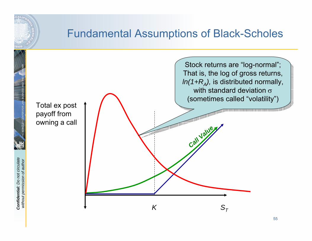
Fundamental Assumptions of Black-Scholes
ST
Total ex post payoff from owning a call
K
Stock returns are “log-normal”; That is, the log of gross returns, ln(1+RA), is distributed normally,
with standard deviation σ (sometimes called “volatility”)
Stock returns are “log-normal”; That is, the log of gross returns, ln(1+RA), is distributed normally,
with standard deviation σ (sometimes called “volatility”)
Call Value
56
Con
fiden
tial:
Do
not c
ircul
ate
with
out p
erm
issi
on o
f aut
hor
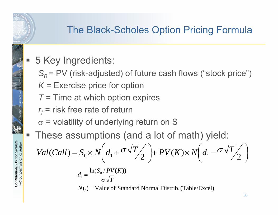
The Black-Scholes Option Pricing Formula
5 Key Ingredients:S0 = PV (risk-adjusted) of future cash flows (“stock price”)K = Exercise price for optionT = Time at which option expiresrf = risk free rate of returnσ = volatility of underlying return on S
These assumptions (and a lot of math) yield:
⎟⎠⎞
⎜⎝⎛ −×+⎟
⎠⎞
⎜⎝⎛ +×= 2)(2)( 110
TdNKPVTdNSCallVal σσ
el)(Table/Exc Distrib. Normal Standard of Value(.)
))(/ln( 01
=
=
NT
KPVSdσ
57
Con
fiden
tial:
Do
not c
ircul
ate
with
out p
erm
issi
on o
f aut
hor
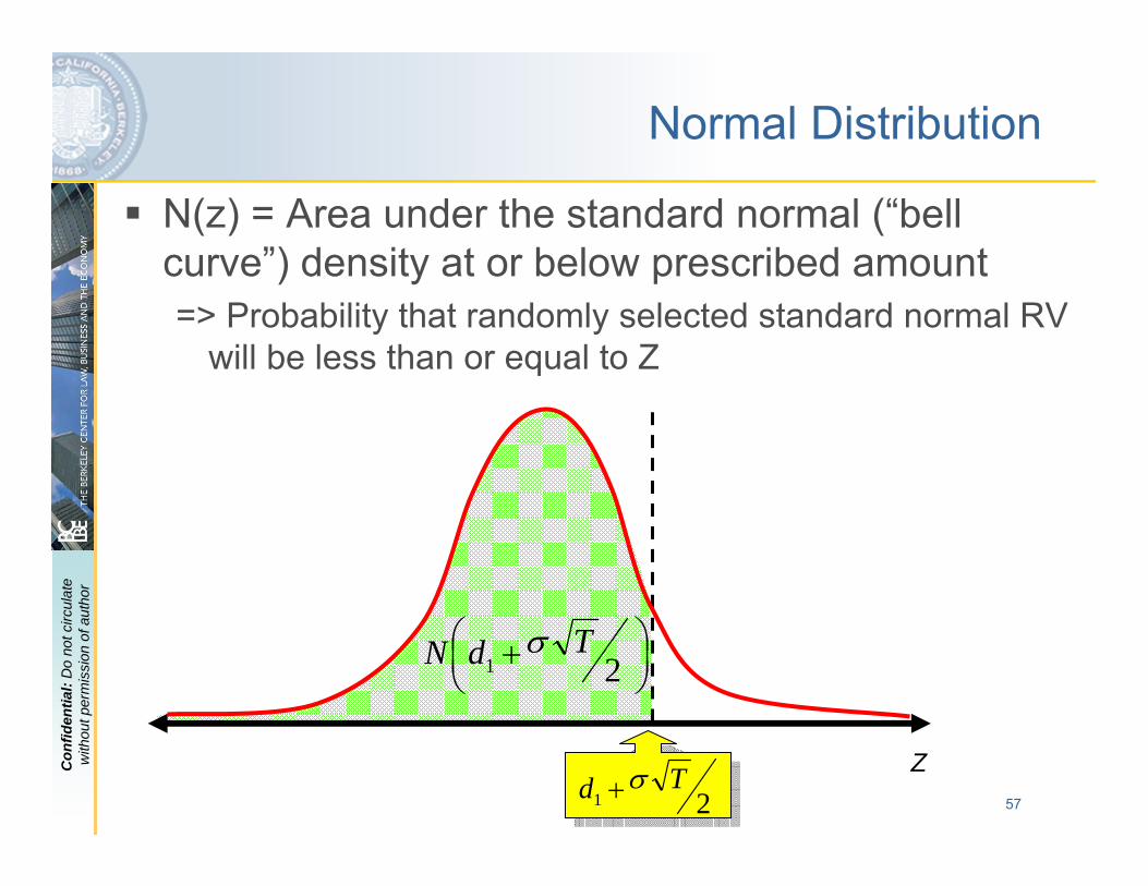
Normal Distribution
N(z) = Area under the standard normal (“bell curve”) density at or below prescribed amount=> Probability that randomly selected standard normal RV
will be less than or equal to Z
Z21
Td σ+
⎟⎠⎞
⎜⎝⎛ + 21
TdN σ
58
Con
fiden
tial:
Do
not c
ircul
ate
with
out p
erm
issi
on o
f aut
hor
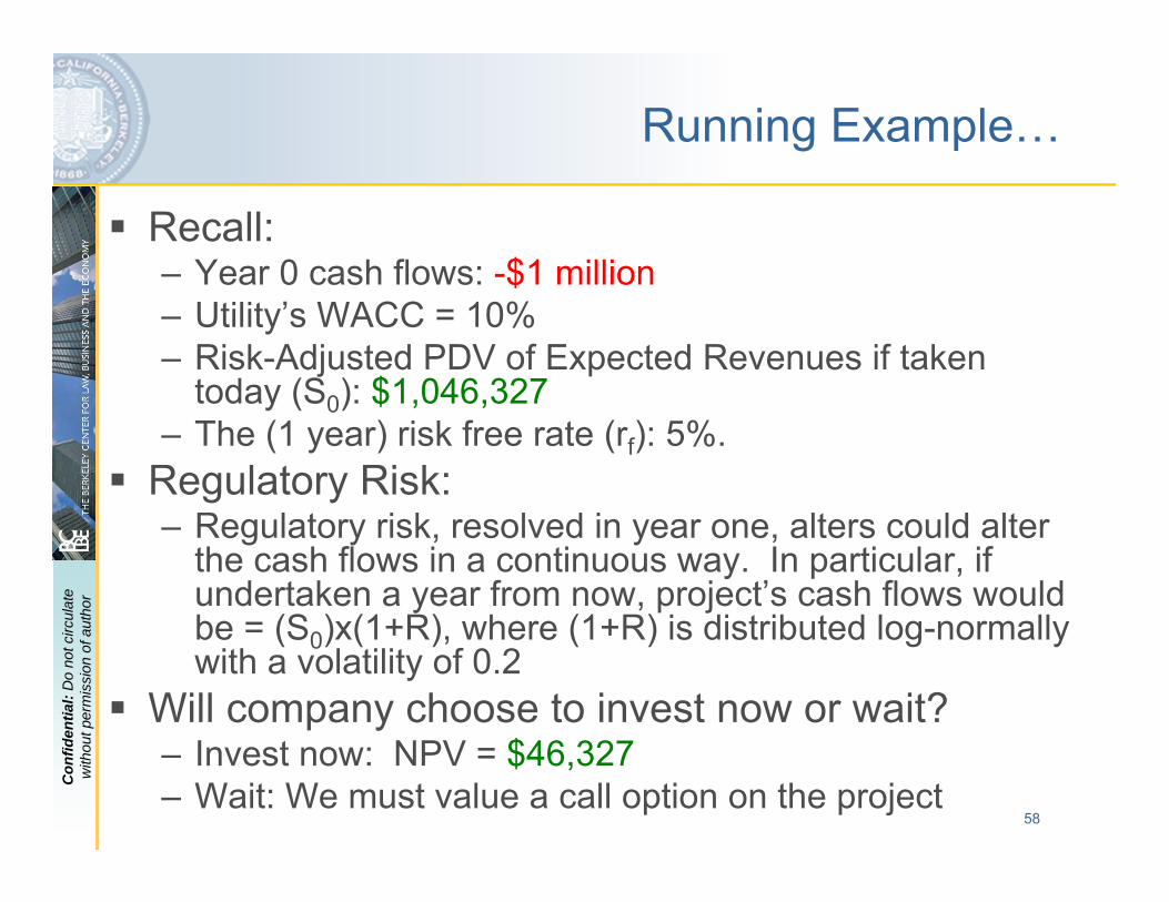
Running Example…
Recall:– Year 0 cash flows: -$1 million– Utility’s WACC = 10% – Risk-Adjusted PDV of Expected Revenues if taken
today (S0): $1,046,327– The (1 year) risk free rate (rf): 5%.
Regulatory Risk:– Regulatory risk, resolved in year one, alters could alter
the cash flows in a continuous way. In particular, if undertaken a year from now, project’s cash flows would be = (S0)x(1+R), where (1+R) is distributed log-normally with a volatility of 0.2
Will company choose to invest now or wait?– Invest now: NPV = $46,327– Wait: We must value a call option on the project
59
Con
fiden
tial:
Do
not c
ircul
ate
with
out p
erm
issi
on o
f aut
hor
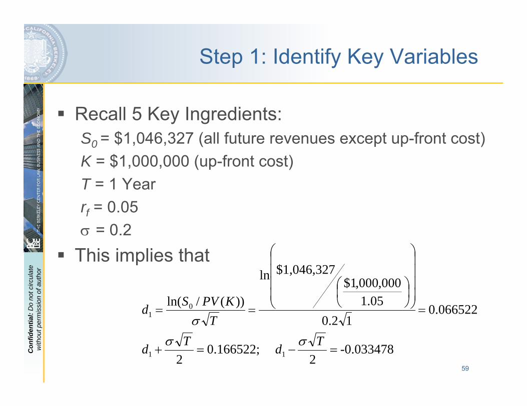
Step 1: Identify Key Variables
Recall 5 Key Ingredients:S0 = $1,046,327 (all future revenues except up-front cost)K = $1,000,000 (up-front cost)T = 1 Yearrf = 0.05σ = 0.2
This implies that
-0.0334782
66522;1.02
665220.012.0
05.1000,000,1$
$1,046,327ln
))(/ln(
11
01
=−=+
=⎟⎟⎟⎟
⎠
⎞
⎜⎜⎜⎜
⎝
⎛
⎟⎠⎞
⎜⎝⎛
==
TdTd
TKPVSd
σσσ
60
Con
fiden
tial:
Do
not c
ircul
ate
with
out p
erm
issi
on o
f aut
hor
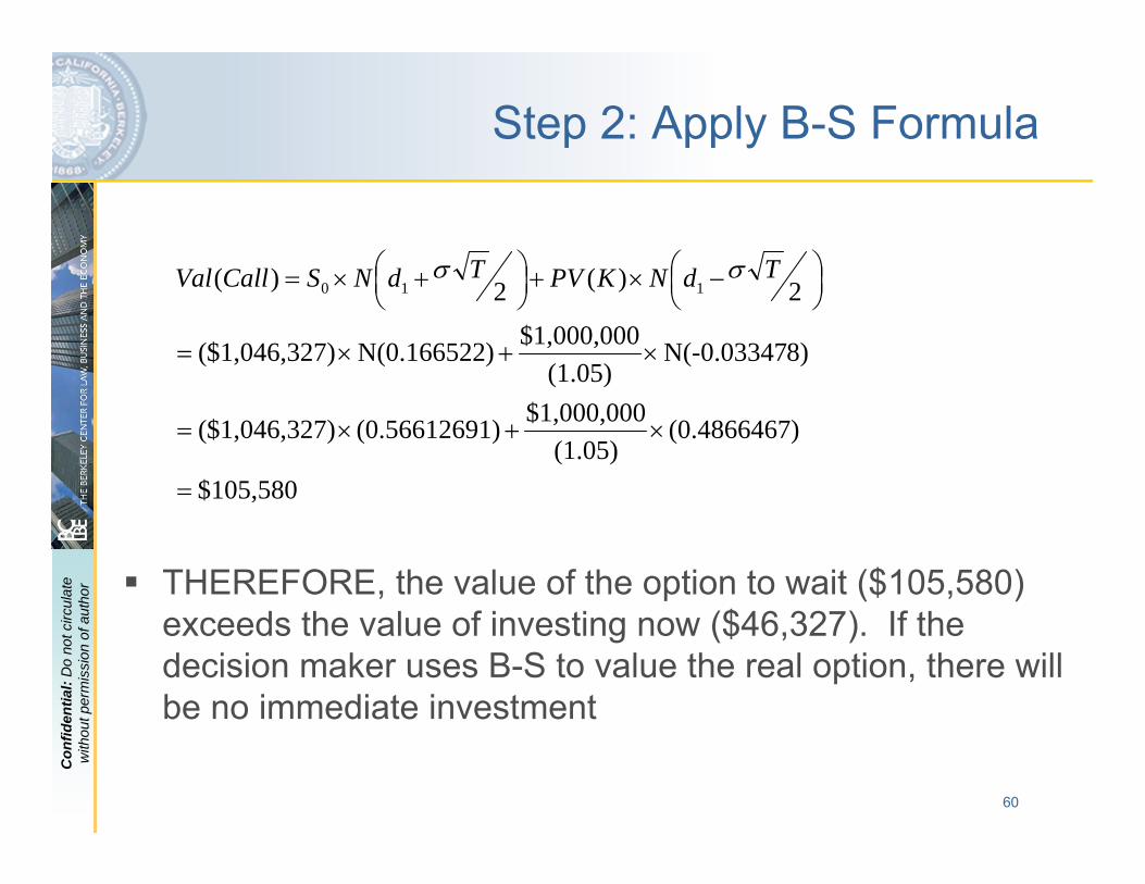
Step 2: Apply B-S Formula
THEREFORE, the value of the option to wait ($105,580) exceeds the value of investing now ($46,327). If the decision maker uses B-S to value the real option, there will be no immediate investment
$105,580
)(0.4866467(1.05)
$1,000,0001)(0.5661269)$1,046,327(
8)N(-0.03347(1.05)
$1,000,000)N(0.166522)$1,046,327(
2)(2)( 110
=
×+×=
×+×=
⎟⎠⎞
⎜⎝⎛ −×+⎟
⎠⎞
⎜⎝⎛ +×= TdNKPVTdNSCallVal σσ

61
Con
fiden
tial:
Do
not c
ircul
ate
with
out p
erm
issi
on o
f aut
hor
Binomial “Lattice” Models
Decision tree-like structure in which value of asset could experience an “up” return (1+R =u > 1), or a “down return (1+R = d < 1).Probabilities of “u” and “d” are given by π and (1-π)– “Risk neutral” probabilities
Value of call at t=0 is simply equal to probability-weighted value of each call at t=1.Very simple structure, but can be adapted to complex environments– Each tree is a simple
computation for a computer– It’s possible to add on many
“branches” of the tree and set the computer to work…
D
U
S1 = d × S0
C1 = max{0, d × S0 - K }
S1 = u × S0
C1 = max{0,u × S0 - K }
π
1-π
S0
D
U
S1 = d × S0
C1 = max{0, d × S0 - K }
S1 = u × S0
C1 = max{0,u × S0 - K }
π
1-π
S0

62
Con
fiden
tial:
Do
not c
ircul
ate
with
out p
erm
issi
on o
f aut
hor
Example: Three Periods
π
1-π
π
1-π
π
1-π
π
1-π
π
1-π
π
1-π
S1 = u3 · S0C1 = max{0, u3 · S0 – K}
S1 = d · u2 · S0C1 = max{0, d · u2 · S0 – K}
S1 = d2 · u · S0C1 = max{0, d2 · u · S0 – K}
S1 = d3 · S0C1 = max{0, d3 · S0 – K}
π
1-π
π
1-π
π
1-π
π
1-π
π
1-π
π
1-π
π
1-π
π
1-π
π
1-π
π
1-π
π
1-π
π
1-π
S1 = u3 · S0C1 = max{0, u3 · S0 – K}
S1 = d · u2 · S0C1 = max{0, d · u2 · S0 – K}
S1 = d2 · u · S0C1 = max{0, d2 · u · S0 – K}
S1 = d3 · S0C1 = max{0, d3 · S0 – K}
63
Con
fiden
tial:
Do
not c
ircul
ate
with
out p
erm
issi
on o
f aut
hor
A Word of Caution
Both the Black-Scholes and the binomial approaches depend on two core assumptions that are probably not satisfied in practice for real options:– Both the option and the stock can be continuously
traded in a frictionless market at zero cost;– There are no restrictions on short selling of any asset
(including borrowing and lending at the risk free rate);This has led some to question their usefulness in valuing real optionsBut there also may be no good practical candidates (e.g., Decision Tree)
64
Con
fiden
tial:
Do
not c
ircul
ate
with
out p
erm
issi
on o
f aut
hor
Rules of Thumb from Options Valuation
In addition to the rules of thumb from risk-adjusted NPV (see above), the option to delay investment may also have valueHolding all else constant, investors are more likely to invest now (instead of delaying) when…
1. …future volatility / uncertainty decreases2. …the risk free rate of return decreases3. …the time horizon for delaying decreases4. …the up-front cost of investment decreases5. …the timing of the + net revenue stream accelerates
Economic factors / policies that bring about (1) – (5) tend to catalyze current investment.
And, vice versa, things that reverse (1) – (5) tend to discourage current investment.
KeyPointKeyPoint
65
Con
fiden
tial:
Do
not c
ircul
ate
with
out p
erm
issi
on o
f aut
hor
End of program
The evolving regulatory state