i

University of British Columbia Electrical and Computer Engineering

EECE 496 Final Report

RS1: Implementation and Test of Software Fading Simulators

November 24th, 2003

Submitted to: Dr. R. Schober Ms. J. Pavelich

Prepared by:

Chiou Perng Ong (33795006)

ii

ABSTRACT Fading is a physical phenomenon associated with transmitted signals in wireless

communications. With the hypothesis of many mathematical models used to

model fading, the Nakagami fading channel model is widely adopted. It is

important to generate Nakagami fading channels for system analysis and design

due to the high accuracy in matching Nakagami model with some experimental

data when compared to other fading models like Rayleigh and log-normal.

Furthermore, Nakagami fading channel can be used to model Rayleigh and

Rician fading with some specially defined parameters, making it a more powerful

model to implement and thus a more significant one to study. In this report, a

correlated Nakagami-m channel is generated with either single-m or multiple-m

fading parameters within the channel’s branches. The philosophy is to generate

Nakagami random variables from independent identically distributed Gaussian

random variables with a set of user-defined parameters such as envelope

correlation, variance and fading parameter. The process includes applying

Chloesky decomposition, Newton Raphson’s iteration, and relating correlated

Gamma random variables to Nakagami random variables. The generated

channel is then tested against the theoretical function to test the accuracy of the

underlying methodology.

iii

TABLE OF CONTENTS Abstract.……………………………………………………………………………….. ii

List of Illustrations.…………………………………………………………………… v

Glossary.………………………………………………………………………………. vi

List of Abbreviations.………………………………………………………………… viii

1.0 Introduction..……………………………………………………………………… 1

2.0 Fading..…………………………………………………………………………… 3

2.1 Signals Fading.…………..………………………………………………. 3

2.2 Nakagami-m Fading………….…………………………………………. 5

3.0 Methodologies and Algorithms..……………………………………………….. 8

3.1 Definition and Notation………………………………………………….. 8

3.2 Single-m Fading Channel.……………………...………………………. 9

3.3 Multiple-m Fading Channel.………………………………..…………... 12

4.0 Results and Discussions.……………………………………………………….. 15

4.1 Single-m Fading Channel.……………………………………………… 15

4.1.1 Covariance Matrix Tester…………………………………….. 16

4.1.2 PDF Plot Tester………………………………………………... 17

4.2 Multiple-m Fading Channel.………………………………..…………... 19

4.2.1 Covariance Matrix Tester…………………………………….. 20

4.2.2 PDF Plot Tester………………………………………………... 22

5.0 Conclusion.……………………………………………………………………….. 25

References...………………………………………………………………………….. 26

iv

Appendix A …………………………………………………………………………… A-1

Appendix B …………………………………………………………………………… B-1

Appendix C …………………………………………………………………………… C-1

Appendix D …………………………………………………………………………… D-1

Appendix E……………………………………………………………………………. E-1

Appendix F……………………………………………………………………………. F-1

Appendix G……………………………………………………………………………. G-1

v

LIST OF ILLUSTRATIONS

Figures:

Figure 1. Mechanism of Radio Propagation in a Mobile Environment….… 3

Figure 2. The pdf of Simulated Data Versus Rayleigh and

Nakagami Distribution…………………………………………………….…….

6

Figure 3. PDF Plot for Single-m Channel, m=2.18……………...…………... 18

Figure 4. PDF Plot for Single-m Channel, m=1………………………...……. 19

Figure 5. PDF Plot for Multiple-m Channel……………………………...…… 23

Figure 6. PDF Plot for Multiple-m Channel, m=10…………………………... G-1

Figure 7. PDF Plot for Multiple-m Channel, m=5……………………………. G-1

Figure 8. PDF Plot for Multiple-m Channel, m=2.18………………………… G-2

Figure 9. PDF Plot for Multiple-m Channel, m=1……………………………. G-2

Tables:

Table 1. Definition of Variables………...……………………………………… 9

Table 2. γρ Versus zρ …………………...…………………………………….. 13

Table 3. Variable Values for Single-m Channel...…………………………… 15

Table 4. zR Versus zR∧

(Single-m Channel)…..…...……………………...….. 16

Table 5. Variable Values for Multiple-m Channel…..…..…………………… 20

Table 6. zR Versus zR∧

(Multiple-m Channel)...………...……………...…….. 22

vi

GLOSSARY

** Note: All definitions are obtained from science dictionary provided by

McGraw-Hill website: http://www.accessscience.com/sci-bin/freesearch [1]

Correlation [STATISTICS] The interdependence or association between two

variables that are quantitative or qualitative in nature.

Correlation coefficient [STATISTICS] A measurement, which is unchanged by

both addition and multiplication of the random variable by positive constants, of

the tendency of two random variables X and Y to vary together; it is given by the

ratio of the covariance of X and Y to the square root of the product of the

variance of X and the variance of Y.

Covariance [STATISTICS] A measurement of the tendency of two random

variables, X and Y, to vary together, given by the expected value of the variable

Doppler effect [PHYSICS] The change in the observed frequency of an

acoustic or electromagnetic wave due to relative motion of source and observer.

Doppler shift [PHYSICS] The amount of the change in the observed frequency

of a wave due to Doppler effect, usually expressed in hertz. Also known as

Doppler frequency.

vii

Envelope [COMMUNICATIONS] A curve drawn to pass through the peaks of a

graph, such as that of a modulated radio-frequency carrier signal.

Fading [COMMUNICATIONS] Variations in the field strength of a radio signal,

usually gradual, that is caused by changes in the transmission medium.

Line of sight [ELECTROMAGNETISM] The straight line for a transmitting radar

antenna in the direction of the beam.

Multipath transmission [ELECTROMAGNETISM] The propagation

phenomenon that results in signals reaching a radio receiving antenna by two or

more paths, causing distortion in radio and ghost images in television. Also

known as multipath.

Probability density function [STATISTICS] A real-valued function whose

integral over any set gives the probability that a random variable has values in

this set

viii

LIST OF ABBREVIATIONS LOS: Line of Sight

PDF: Probability Distribution Function

IID: Independent Identically Distributed

1

1.0 INTRODUCTION This report presents the analysis of the Nakagami-m signal fading* model in

wireless communication, through multipath* propagation channels. The objective

of this project is to simulate the Nakagami-m fading model with a MATLAB

program. The program, when called in the MATLAB workspace, will generate

random variables (RVs) that follow the Nakagami-m distribution. The user will

have to define constraints like fading parameter, envelope* correlation* matrix

and variance vector, to generate the desired Nakagami-m vectors.

Fading has a negative effect on wireless communication as it causes the

amplitude of transmitted signals to decay during transmission. Software

simulation of this phenomenon is desirable because of the inflexibility and high

cost incurred in hardware experimentations. Thus, this project allows high

flexibility in the investigation of the Nakagami-m fading model by varying the

user-defined parameters, and it is relatively inexpensive compared to building

hardware circuits. Although many papers have been written about the

generation of correlated Nakagami-m channels, an open source where such a

simulator can be downloaded for free does not exist. Thus the creation of such a

simulator is essential for the testing of wireless systems.

This project consists of two groups doing different fading models. Group one,

consisting of Jeffrey Choy and Jonathan Wong, is working on Rayleigh fading in

* This and all subsequent terms marked with an asterisk are defined in Glossary, pp vi-vii

2

a time variant channel, while Group two, consisting of Chiou Perng Ong and

Michael Chan, is working on Nakagami-m fading in a single channel with multiple

fading parameters. For the Nakagami group, two programs have been written to

generate Nakagami-m fading channel with either single or multiple-m fading

parameters. Four testing programs have also been written to test the accuracy

of the generator program against the theoretical Nakagami-m fading channel.

Due to the highly statistical nature of the program, there are many ways in which

Nakagami-m RVs can be estimated, given the allowable error in the generated

data. This project thus uses the algorithm taken from literature obtained from

communication journals from the IEEE. This report will attempt to explain the

fundamentals of fading and the algorithm used to generate the Nakagami-RVs,

and also the tester programs created to test the accuracy of the estimation used.

This report is divided into the following sub-sections. It will first present the

concept of fading and Nakagami-m model, followed by the methodology and

algorithm used to create the programs and lastly the results and comparison of

the generated data with the theoretical data.

3

2.0 FADING This section will attempt to introduce signal fading. The first sub-section will

discuss the theory and science behind the fading phenomenon, while the second

sub-section will discuss a particular kind of fading that is of concern in this

project: The Nakagami-m Fading.

2.1 Signals Fading Radio waves propagate through the environment from a transmitting antenna to

a receiving antenna. During this transmission process, the waves experience

absorption, diffraction, reflection, refraction, and scattering [2]. Unless there is a

direct Line-of-Sight* (LOS) between the transmitting antenna and the receiving

antenna, wave propagation will only be possible through a series of diffraction,

reflection and scattering. Due to this physical restriction, waves will arrive at the

receiving antenna via different paths with different time delays creating a

multipath situation shown in Figure1.

Figure 1. Mechanism of Radio Propagation in a Mobile Environment. Source: [2]

4

These multipath waves, each having a randomly distributed amplitude and

phase, will combine at the receiver, giving rise to a resultant received signal that

fluctuates with time and space. This fluctuation in the signal amplitude is thus

called fading.

Fading can be categorized into small-scale fading and large-scale fading. The

former is observed over distances of about half a wavelength, whereas the latter

is due to movement over distances large enough to cause a significant variation

in the overall wave propagation path. These two classes of fading can then be

sub-categorized into different kinds of fading, which are not within the scope of

this report.

Several mathematical models have been developed to study the fading

phenomenon so as to improve the quality of wireless communication. Examples

of such mathematical models are Rayleigh fading, Rician fading and Nakagami

fading. Knowing how waves fade in an urban setting enables telecommunication

companies to effectively set up rebroadcast and relay stations, increasing its

coverage area. The study of fading may be applied in this manner, amongst

others.

5

2.2 Nakagami-m Fading This paper focuses on the study of how to create and simulate a Nakagami-m

fading channel. The reason of study being that the Nakagami-m fading

distribution model is one of the most versatile, in the sense that it is more flexible

and accurate in matching some experimental data than the Rayleigh, log-normal,

or Rician distributions [3]. In studies conducted by Suzuki and Aulin, among all

the other models mentioned above, the Nakagami distribution gave the best fit to

some urban multipath data [3]. Thus, it is essential to generate correlated

Nakagami fading channels for laboratory testing of wireless systems.

For a general I-branch diversity system in Nakagami fading environment, the

fading envelope variable xi of the ith (1 ≤ i ≤ I) branch follows the Nakagami-

distribution [4]:

2 1 22( ) ( ) exp( )( )

i im mi ii i

i i i

m mf x xi xm P P

−= −Γ

, (1)

where Γ(• ) is the Euler Gamma function and

2[ ]i iP E x= , 2 2

2 2 2

[ ][( ( )) ]

ii

i i

E xmE x E x

=−

. (2)

Equation (1) will be the theoretical probability distribution function* (pdf) for our

study of the Nakagami-m fading channel in this paper. The algorithm described

in the next section will explain the approach this paper has adopted for

generating Nakagami fading vectors.

6

In particular, for m=1, the Nakagami-m distribution reduces to a Rayleigh

distribution. And for 1< m < 2, the Nakagami-m distribution tends to a Rician

distribution [2]. The relation between Rayleigh and Nakagami distribution is

shown in Figure 2 below.

Figure 2. The pdf of Simulated Data Versus Rayleigh and Nakagami Distribution. Source: [2]

7

The Rayleigh density function can be created by calculating the Rayleigh

parameter from the moments of the envelope data described by:

1

1( ) cos( ) cos( )

N

i c di i d c di

s t a w t w t k w t w tφ−

== + + + +∑ (3)

where s(t) is the transmitted signal, dk is the strength of the direct component,

dw is the Doppler shift* along the LOS path, and diw are the Doppler shifts along

the indirect paths [2]. More discussions on Rayleigh distribution can be found in

the report written by the other group on this project, RS1 (by Jeffrey Choy and

Jonathan Wong).

8

3.0 METHODOLOGIES AND ALGORITHM

This section describes the methodologies and algorithms that were used to

generate Nakagami-m fading signals. The aim of the software program is to

generate an n-by-1 correlated Nakagami vector z with fading parameter m and

covariance matrix zR . As directly generating a Nakagami sequence is extremely

difficult, an indirect approach that follows the philosophy illustrated below will be

used [3]:

2 (1/ 2)( ) ( )Lk k ke x u y z• ∑ •

→ → → → (3)

where ke is a sequence of independent identically distributed (iid) Gaussian

random variables, xk is a set of independent Gaussian vectors, y vector follows

gamma distribution and z vector follows a Nakagami distribution. Due to the

large amount of equations and notations being presented in this paper, the next

subsection will attempt to give readers a reference as to how data is being

presented. The approach used for the single-m and multiple-m fading channel

will then be discussed separately in two sections subsequent to the notation

subsection.

3.1 Definition and Notation First, the following three notations

~ (0, ) , ~ ( , ) , ~ ( , )x y zx N R y GM m R z NK m R (4)

9

are used to indicate that the vectors x, y and z follow a joint Gaussian, gamma

and Nakagami distribution as depicted by N, GM and NK respectively. The other

variables are summarized in the table below:

Table 1 Definition of variables. ,zC Cγ Envelope Correlation Matrix

, ,x zR R Rγ Covariance* Matrix

,z γρ ρ Correlation coefficient*, indices of respective C

zp Variance vector

m Nakagami-m fading parameter

N Number of samples to be generated

P Power of a branch in the channel

All variables are in the form of vectors or matrices unless a certain index entry

within a matrix is specified or otherwise specified.

3.2 Single-m Fading Channel The main approach to this algorithm is to implement (3) by exploiting the

relationship between ,x zR R and Rγ illustrated by z y xR R R→ → (5)

With the user’s input of zC and zp , the user is able to find zR using

( , ) cov( , ) ( , ) var( ) var( )i j i j i jR r r r r i j r rρ= = ∗ × . (6)

10

This relationship between covariance, correlation coefficient and variance is

always true for any RVs. Hence to find Rγ , one uses the relationship between

the Nakagami and Gamma correlation coefficient that is given by

2 1

( , ) ( ( ) , ( ) )

( , ){ ( , ; ; ( , )) 1}2 2

n nn i j corr z i z j

n nm n F m v i j

ρ

ϕ= − − − (7)

where ρn(i, j) is the correlation coefficient of the Nakagami vectors, and v(i, j) is

the correlation coefficient of the Gamma vectors. And where

2

2

( )2( , )

( ) ( ) ( )2

baa b ba a b a

ϕΓ +

=Γ Γ + − Γ +

. (8)

And the hypergeometric function is given by

2 10

( ) ( )( , ; ; ) ,( ) !

nn n

n n

a b zF a b c zc n

∞

=

=∑ (9)

with ( ) ( 1)...( 1)a n a a a n= + + − and 0( ) 1a = . However, since the user input

specifies the correlation and variance of the desired Nakagami distribution, the

following equations allows the computation of v(i, j) from ρn(i, j).

2 11 1( ( , )) ( ,1){ ( , ; ; ( , )) 1}2 2

f v i j m F m v i jϕ ρ− − − − (10)

2 1( ,1) 1 1( ( , )) { ( , ; 1; ( , ))}4 2 2mf v i j F m v i jm

ϕ= − − + (11)

1( )

( )i

i i

i

f vv vf v

+ = − (12)

11

This is a Newton-Raphson iterative process, with v0 = ρ. The process should

converge within a few steps, and the difference ∆v is set to be 1x10-6 in the

MATLAB program.

Similarly, by applying (6), the user can find xR directly from zR using the

equations defined in (13) and (14):

1/ 2

var[ ( )],( , )

{var[ ( )]var[ ( )] ( , ) },x

z k k lR k l

z k z l v k l k lζ

ζ=

= ≠ (13)

where

1212

2

var[ ( )] ( , )

( )1 1[1 ]2 ( )

zz k R k km

m m mζ −

=

Γ += −

Γ . (14)

Now that the relationship between zR , Rγ and xR has been found, the user is

ready to generate x, y and z vectors.

xk can then be generated using the relationship as illustrated below:

†,~ (0,1) xL R LLk k ke N x Le= → = (15)

where L can be found by applying Cholesky decomposition to xR .

Consequently y can be calculated by using

22

1

2 21

1

, 2 int

,

m

kk

p

k pk

x m egery

x x otherwiseα β

=

+=

== +

∑

∑ (16)

12

where p is the integer part of 2m (i.e. floor(2m)). Equation (17) and (18) shows

the computation of α and β.

2 2 ( 1 2 )( 1)

pm pm p mp p

α + + −=

+ (17)

2m pβ α= − (18)

This method of generating y is estimated from the result generated from Direct

Sum Decomposition, as compared to Cholesky decomposition. Due to the fact

that direct sum decomposition works on the assumption that 2m is an integer,

there is a need for correction terms and coefficients as shown in (16) for

2m≠integer.

Lastly, Nakagami vector z is obtained by

(1/ 2)z y= (19)

The MATLAB code for generating a single-m Nakagami channel with N number

of samples is included in Appendix A. The user will have to, as mentioned

earlier, input zC , zp , m, N in the form: naka(C, p, m, N). The number of

branches in this single-m channel will be determined by the size of zC .

3.3 Multiple-m Fading Channel Generating a multiple-m fading channel is basically, and in theory, the same as

generating a single-m fading channel. In the previous section, a multiple-branch

13

single-m Nakagami fading channel has been generated, where the number of

branches is determined by the size of zC (n by n matrix means an n-branch

channel). Likewise in this section, a multiple-branch Nakagami-m fading channel

will be generated, with the difference now that each branch will have a unique

fading parameter m.

The other difference is with equation (7). In a single-m channel, γρ is derived by

applying (10)-(12). However, there is no such analytical formula for a multiple-m

channel. Therefore, it is necessary to determine the method in which the user

can find yR .

As described in [4], the way to find the relationship between zR and yR is by

generating a set of Gamma RVs with known correlation coefficients between

different branches, and then the square root of the Gamma RVs to obtain the

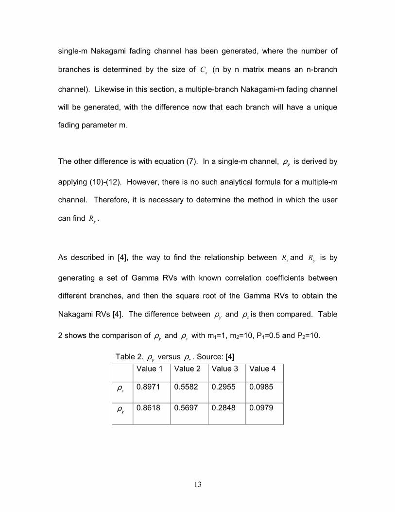
Nakagami RVs [4]. The difference between γρ and zρ is then compared. Table

2 shows the comparison of γρ and zρ with m1=1, m2=10, P1=0.5 and P2=10.

Table 2. γρ versus zρ . Source: [4] Value 1 Value 2 Value 3 Value 4

zρ 0.8971 0.5582 0.2955 0.0985

γρ 0.8618 0.5697 0.2848 0.0979

14

Since the differences in the values are small, the approximation zγρ ρ≈ can be

made. However, since the generation of γρ described in (7), (10), (11) and (12)

can also be substituted as zγρ ρ≈ [4], the approach to generating γρ from zρ in

this paper is kept to be the same as that described in section 3.1.

Appendix B contains the MATLAB code that is used to generate a multiple-m

fading channel. The user input will be zC , zp , [m], N in the form: nakamulti(C, p,

m, N). The difference between nakamulti.m and naka.m is that [m] is a vector

whose size is determined by the size of zC . That is, if zC is an n n× matrix, then

[m] will be a 1 n× vector.

15

4.0 RESULTS AND DISCUSSION The results generated from section 3.2 and section 3.3 are tested and compared

against the theoretical function mentioned in (1) and (6). Four separate test

programs (two each for single-m and multiple-m channel) were written to

compare the generated covariance matrix, zR∧

with specified zR , and the

generated pdf with the pdf function described in (1). The test programs will be

described in subsequent sub-sections, together with specific comparisons made

to the theoretical values.

4.1 Single-m Fading Channel The following variable values are used for the testing programs in the testing of

the single-m fading channel.

Table 3. Variable values for Single-m Channel Variable Value

zC

1 0.795 0.604 0.3720.795 1 0.795 0.6040.604 0.795 1 0.7950.372 0.604 0.795 1

zp [2.16, 1.59, 3.32, 2.78]

m 2.18, 1

N 10000

16

A 4-branch single-m fading channel will be generated since zC is a 4 4× matrix.

Two m values are chosen to illustrate the difference in the shape of the pdf when

the fading parameter changes, and to simulate a Rayleigh distribution.

4.1.1 Covariance Matrix Tester A tester program is written to test the accuracy of the estimated Nakagami

covariance matrix ( zR∧

) with the specified covariance matrix ( zR ). The specified

covariance matrix can be calculated by applying (6) while the estimated matrix

can be found by simply calculating the sample covariance from the RVs

generated. The MATLAB code for this tester is attached in Appendix C for

reference.

The comparison is shown in Table 4 below.

Table 4. zR versus zR∧

(Single-m Channel). m=2.18 m=1

zR

2.1600 1.4733 1.6175 0.91161.4733 1.5900 1.8266 1.26991.6175 1.8266 3.3200 2.41520.9116 1.2699 2.4152 2.7800

2.1600 1.4733 1.6175 0.91161.4733 1.5900 1.8266 1.26991.6175 1.8266 3.3200 2.41520.9116 1.2699 2.4152 2.7800

zR∧

2.0915 1.4187 1.5407 0.86731.4187 1.5412 1.7632 1.23871.5407 1.7632 3.2368 2.36310.8673 1.2387 2.3631 2.7346

2.1563 1.4653 1.6113 0.91371.4653 1.5756 1.8153 1.25601.6113 1.8153 3.2859 2.37270.9137 1.2560 2.3727 2.7427

17

Percentage

Error

3.1712 3.7084 4.7429 4.86133.7084 3.0662 3.4700 2.45624.4729 3.4700 2.5063 2.15944.8613 2.4562 2.1594 1.6340

0.1692 0.5434 0.3825 0.23210.5434 0.9036 0.6150 1.09100.3825 0.6150 1.0271 1.76150.2321 1.0910 1.7615 1.3420

From the percentage error calculated, it can be concluded that the estimated

Nakagami RVs varies within 5% of the specified RVs. That is to say, the overall

positioning of the generated RVs are within 5% of the expected RVs since

covariance is the measure of how closely two different sets of RVs deviates from

their mean together. It can also be observed that when m increases,

zR∧

increases too. This may primarily be due to equation (7) and (16), as

generation of gamma RVs are related to the value of m.

4.1.2 PDF Plot Tester A tester program is written to compare, graphically the difference between pdf of

the generated RVs and the expected pdf function. The MATLAB code is

attached as Appendix D for reference.

The expected pdf function can be calculated by plotting (1). The iP term in (1) is

calculated using

( , )i iP m C i iγ= ∗ (20)

21222

2

( )var [ ( , )] 1( , ) var[ ( , )] 1( )mz i iC i i y i i

m m mγ

− Γ +

= = − Γ , (21)

18

where var[z(i, j)] are the diagonal elements of zR , which may be calculated from

user specified zC and zp . Since correlation is not important in testing the pdf

accuracy, the average power of the four branches is used instead. On the other

hand, the estimated pdf can be plotted using the function ksdensity available

from MATLAB.

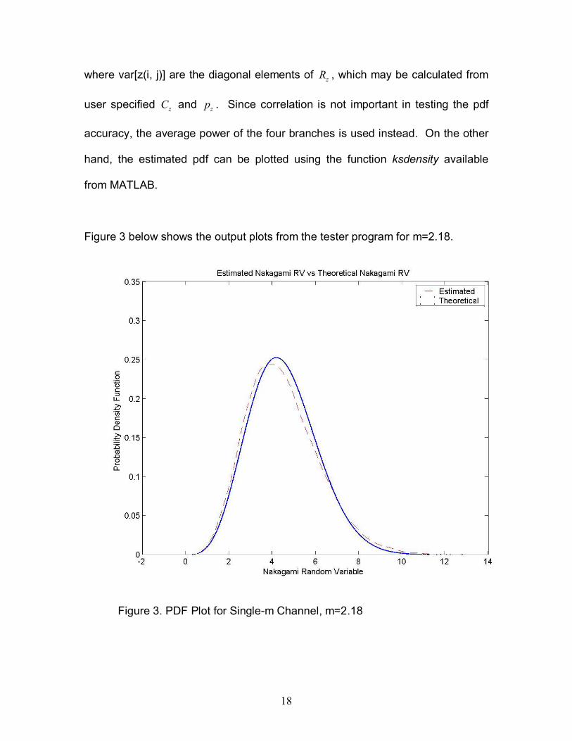
Figure 3 below shows the output plots from the tester program for m=2.18.

Figure 3. PDF Plot for Single-m Channel, m=2.18

19

Figure 4 below shows the pdf plot for m=1.

Figure 4. PDF Plot for Singel-m Channel, m=1

It may be observed that the two pdfs are very close together, proving that the

estimated function is a legitimate approximation.

4.2 Multiple-m Fading Channel The following variable values are used for the testing programs in the testing of

the multiple-m fading channel.

20

Table 5. Variable values for Multiple-m Channel. Variable Value

zC

1 0.795 0.604 0.3720.795 1 0.795 0.6040.604 0.795 1 0.7950.372 0.604 0.795 1

zp [2.16, 1.59, 3.32, 2.78]

m [10, 5, 2.18, 1]

N 10000

A 4-branch multiple-m fading channel will be generated since zC is a 4 4× matrix.

The [m] values are chosen from a wide range to enable a comparison between

branches with distinctly different fading parameters to be made.

4.2.1 Covariance Matrix Tester A similar tester program is written to test the accuracy of the estimated Nakagami

covariance matrix ( zR∧

) with the specified covariance matrix ( zR ) as mentioned in

section 4.1.1. The specified covariance matrix can be calculated by applying (6)

while the estimated matrix is calculated using a slightly different method. The

MATLAB code is attached as Appendix E for reference.

When the method used in section 4.1.1 is used to the estimated covariance

matrix for a multiple-m channel, there are trials when the percentage error

calculated can be as big as 60% between some branches. Although the sample

21

covariance method should work regardless of the value of m, the computed

result shows otherwise. One possible cause could be a wrongly written sample

covariance code. This exact problem could not be correctly determined at the

time this report was written although through the process of elimination, it is

certain that the problem was not with the generated RVs. This conclusion is

derived from the fact that the pdf plots attached as Appendix G show that for

every branch in the channel, the Nakagami RVs are correctly generated as the

plots are very close to the expected pdf.

The revised method of finding the covariance matrix adds an additional step to

the algorithm described in section 4.1.1. Since only the off-diagonal elements in

the covariance matrix are affected by the error, the revised method assumes that

the correlation coefficients of the generated RVs are the same as the specified

one, i.e. z zρ ρ∧

= , where zρ is the entry in the user specified zC . Next, a new

zR∧

is generated using (6) by assuming var[z(i,i)] as the diagonal elements of the

previously generated covariance matrix.

22

The comparison is shown in Table 6 below.

Table 6. zR Versus zR∧

(Multiple-m Channel). M=[10, 5, 2.18, 1]

zR 2.1600 1.4733 1.6175 0.91161.4733 1.5900 1.8266 1.26991.6175 1.8266 3.3200 2.41520.9116 1.2699 2.4152 2.7800

zR∧

2.1685 1.4774 1.6096 0.91511.4774 1.5926 1.8156 1.27331.6096 1.8156 3.2749 2.40320.9151 1.2733 2.4032 2.7904

Percentage Error 0.3915 0.2773 0.4874 0.38250.2773 0.1632 0.6006 0.26830.4874 0.6006 1.3587 0.49630.3825 0.2683 0.4963 0.3735

Using the revised method, we can see that the estimated zR∧

is very close to the

specified zR , which should be the correct observation. It is only conclusive that

the generated RVs are accurate within the branch, as the off-diagonal elements

of zR measures the difference between branches.

4.2.2 PDF Plot Tester A tester program is written to compare, graphically the difference between pdf of

the generated RVs and the expected pdf function. The MATLAB code is

attached as Appendix F for reference.

23

This tester program is essentially the same as that described in section 4.1.2,

except that the power for individual branch is calculated using (20) and (21).

There is no need to take the average power since the pdf plot for each branch is

required.

Figure 5 below shows the pdf plot generated from the tester program. An

enlarged version of Figure 5 can be found in Appendix G attached.

Figure 5. PDF Plot for Multiple-m Channel

24

It may be observed that regardless of the value of m, the generated Nakagami

RVs are very close to the expected RVs. Thus, within branches, the estimation

is a good one. It can therefore be concluded that the algorithm used to generate

the multiple-m fading channel has been correctly implemented despite the fact

that the covariance between branches behaved unexpectedly.

25

5.0 CONCLUSION This report presented the analysis of the Nakagami-m signal fading model in

wireless communication, through multipath propagation channels. A total of two

generator programs and four testers programs have been written to generate the

Nakagami-m fading channel and to test the accuracy of the generated channel.

From the comparisons made between the generated and specified covariance

matrices, the conclusion can be drawn that the algorithms presented in [3] and

[4] are good estimates of the actual Nakagami-m fading channel. Furthermore,

from the comparisons made between the generated pdfs and the expected pdfs,

it is conclusive that the generated RVs behave within the limits of the Nakagami-

m distribution.

Other than the inconclusive part where the generated covariance between

different branches in a multiple-m channel differs too much from the specified

values, this paper has presented an accurate algorithm and coding required for

generating a correlated Nakagami-m fading channel for laboratory simulations.

26

REFERENCES: [1] McGraw-Hill website: http://www.accessscience.com/sci-bin/freesearch

[2] Gayatri S. Prabhu and P. Mohana Shankar, “Simulation of Flat Fading

Using MATLAB for Classroom Instruction,” IEEE Transaction on Education,

vol. 45, No. 1, pp. 19-25, Feb. 2002.

[3] Q. T. Zhang, “A Decomposition Technique for Efficient Generation of

Correlated Nakagami Fading Channels,” IEEE Journal on Selected Areas

in Communications, vol. 18, No. 11, pp. 2385-2392, Nov 2000.

[4] Zhefeng Song, Keli Zhang and Yong Liang Guan, “Generating Correlated

Nakagami Fading Signals with Arbitrary Correlation and Fading

Parameters,” IEEE