university of alberta · characterization of stable delamination growth in fiber-reinforced...

University of Alberta

Characterization of Stable Delamination Growth in Fiber-reinforced Polymers using

Analytical and Numerical approaches

by

Tsegay Belay

A thesis submitted to the Faculty of Graduate Studies and Research in partial fulfillment

of the requirements for the degree of

Master of Science

Department of Mechanical Engineering

©Tsegay Belay

Spring 2013

Edmonton, Alberta

Permission is hereby granted to the University of Alberta Libraries to reproduce single copies of this thesis

and to lend or sell such copies for private, scholarly or scientific research purposes only. Where the thesis is

converted to, or otherwise made available in digital form, the University of Alberta will advise potential

users of the thesis of these terms.

The author reserves all other publication and other rights in association with the copyright in the thesis and,

except as herein before provided, neither the thesis nor any substantial portion thereof may be printed or

otherwise reproduced in any material form whatsoever without the author's prior written permission.

Abstract

This thesis discusses methodologies for the prediction of stable delamination

development in fiber-reinforced composites in pure fracture modes using analytical and

numerical methods.

A new test method, named internal-notched-flexure (INF) test, has recently been

proposed to quantify mode II interlaminar fracture toughness of fibre composites.

Previous investigation has shown that unlike any of the existing test methods, the INF

test generates unconditionally stable delamination growth. This thesis discusses a follow-

up study that revises the analytical expressions for compliance (C) of INF specimen and

its energy release rate for delamination (G). The main improvement in the current

approach is to take into account load in the overhanging section of the specimen; while in

the previous approach, the overhanging section was assumed to be load-free. Validation

of the revised expressions is through comparison of the initial specimen stiffness with

that from a finite element (FE) model of the INF specimen. The virtual INF specimen has

cohesive elements in the interlaminar region to simulate the delamination growth, from

which extent of damage in front of the crack tip can be quantified. Results from FE

model suggest that an extensive damage exists at the crack tip before delamination

growth commences. Therefore, the use of a physical crack length in the analytical

expression for G may severely overestimate the interlaminar fracture toughness. Instead,

an effective crack length should be used. Expression for G based on the effective crack

length yields a value that is very close to the input critical energy release rate (Gc) for the

cohesive elements. The study concludes that load in the overhanging section should be

considered for deriving the analytical expressions for C and G of the INF specimen, and

an effective crack length should be used to calculate the Gc value from the analytical

expression.

In addition to the above work, the study also touches on a finite element approach

based on continuum solid elements with an elastic-plastic damage material property. The

approach was proposed to simulate crack growth in the interlamianr region of FRP, but

should also be applicable to other crack growth phenomena. In this approach, solid

elements are used to simulate crack growth, based on criteria that are a combination of all

stresses, in order to take into account the effect of in-plane normal stress on the damage

initiation. The criterion for delamination propagation is defined based on critical strain

energy. The approach was implemented in a finite element code and was applied to pre-

cracked composites to illustrate its feasibility to simulate the crack development.

Acknowledgements

I am very grateful to my supervisor, Dr. Jar and co-supervisor Dr. Cheng, for their

guidance throughout the course of my MSc study. Without their unreserved support,

continued advice and valuable suggestions on critical problems, it would have been

difficult to complete my study. I also would like to extend my sincere thanks to my

friends Souvenir Mohammed, Scott McKinney, Zahou Yang and Feng Yu for their

encouragement and help. Finally, I express my heartfelt gratitude to my family for their

unreserved love and constant encouragement during my whole life.

Table of Content

Chapter 1 Introduction..................................................................................................... 1

1.1 Background .................................................................................................................. 1

1.2 Purpose and scope of study .......................................................................................... 3

1.3 Structure of thesis ......................................................................................................... 4

Chapter 2 Analytical Prediction of Stable Delamination Growth in Internal-Notched

Flexure (INF) Test............................................................................................................. 5

2.1 Introduction .................................................................................................................. 5

2.2 Compliance Method ................................................................................................... 11

2.2.1 The Timoshenko Beam Theory ......................................................................... 11

2.2.2 The Energy Release Rate for INF Test ............................................................ 12

2.3 Prediction of Load-Displacement Curve for INF test ................................................ 29

2.4 Prediction of Delamination Growth Rate for INF Test and Discussion .................... 30

2.5 Concluding Remarks .................................................................................................. 33

Chapter 3 Finite Element Simulation of Stable Delamination Development ............ 34

3.1 Introduction ................................................................................................................ 34

3.2 Cohesive Elements .................................................................................................... 38

3.2.1 Finite Element Model of INF Specimen using Cohesive Elements .................. 38

3.3 Elastic-Plastic damage material model ....................................................................... 48

3.3.1 Constitutive relationship .................................................................................... 49

3.3.2 Delamination initiation criterion ....................................................................... 57

3.3.3 Delamination evolution law .............................................................................. 58

3.4 Application to pre-cracked composites ...................................................................... 59

3.4.1 The DENT test ................................................................................................... 60

3.4.2 The DCB test ..................................................................................................... 66

3.4.3 The INF test ....................................................................................................... 70

3.5 Conclusions ................................................................................................................ 75

Chapter 4 Conclusions and Future Work .................................................................... 77

4.1 Summary and Conclusions ........................................................................................ 77

4.2 Future work ................................................................................................................ 79

References ........................................................................................................................ 80

List of Figures

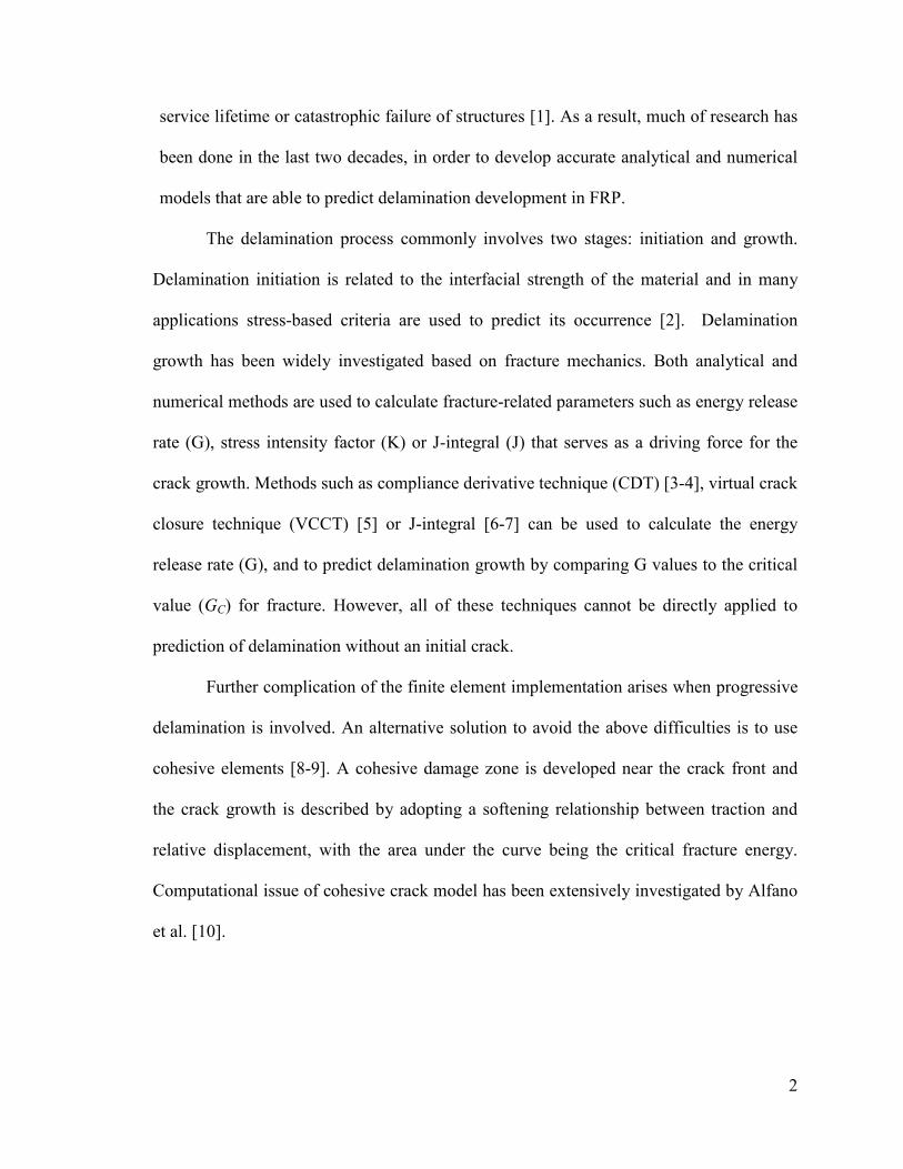
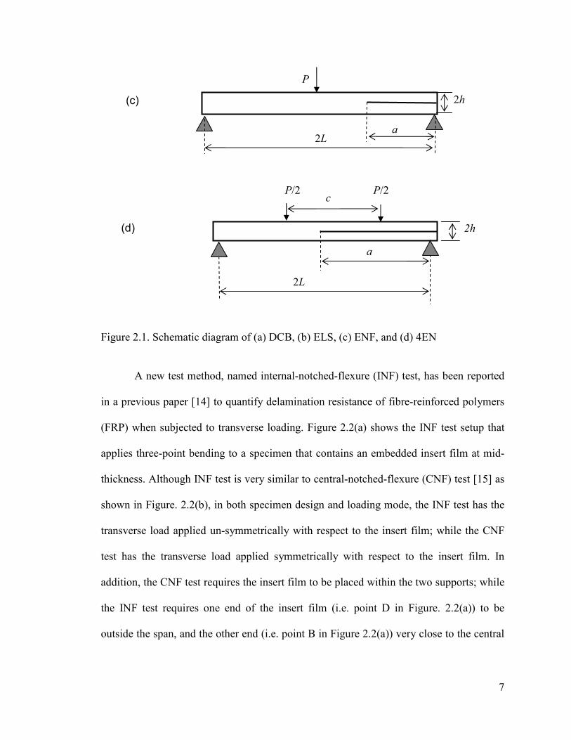
Figure 2.1 Schematic diagram of (a) DCB, (b) ELS, (c) ENF, and (d) 4ENF ................ 7

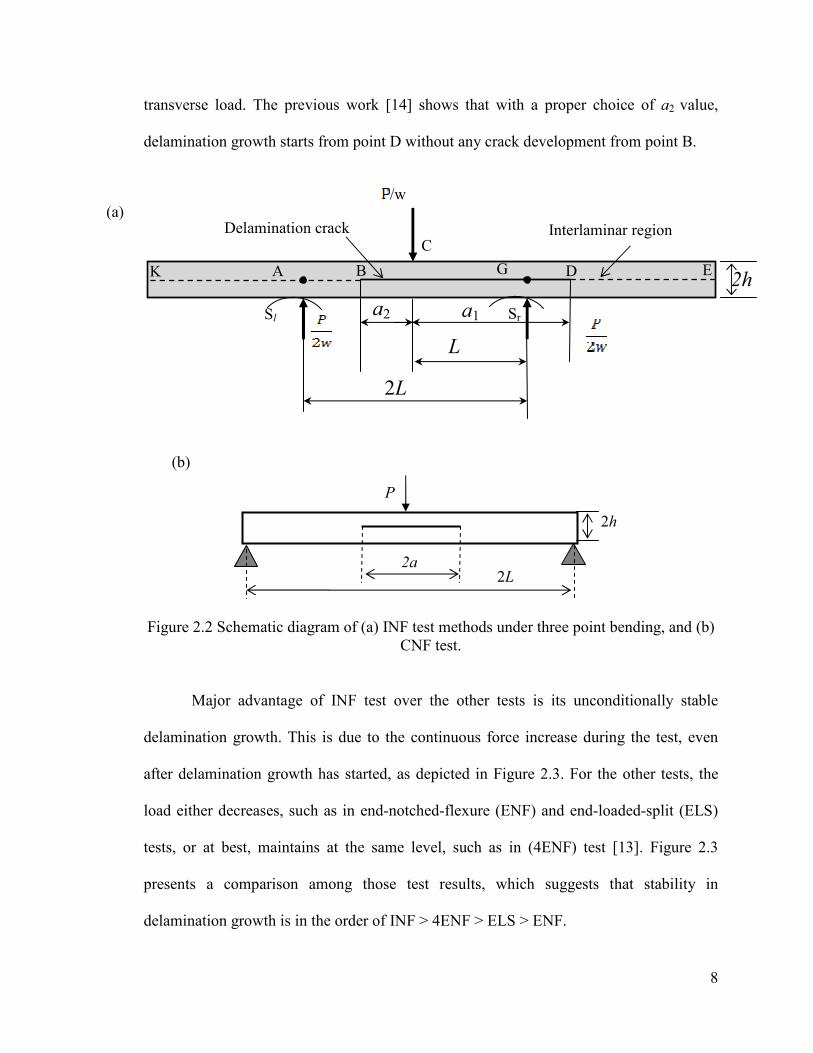
Figure 2.2 Schematic diagram of (a) INF test methods under three point bending, and

(b) CNF test.................................................................................................... 8

Figure 2.3 Schematic diagram of load-displacement plots from five mode II

delamination tests........................................................................................... 9

Figure 2.4 Deformation of Timoshenko beam. ............................................................. 12

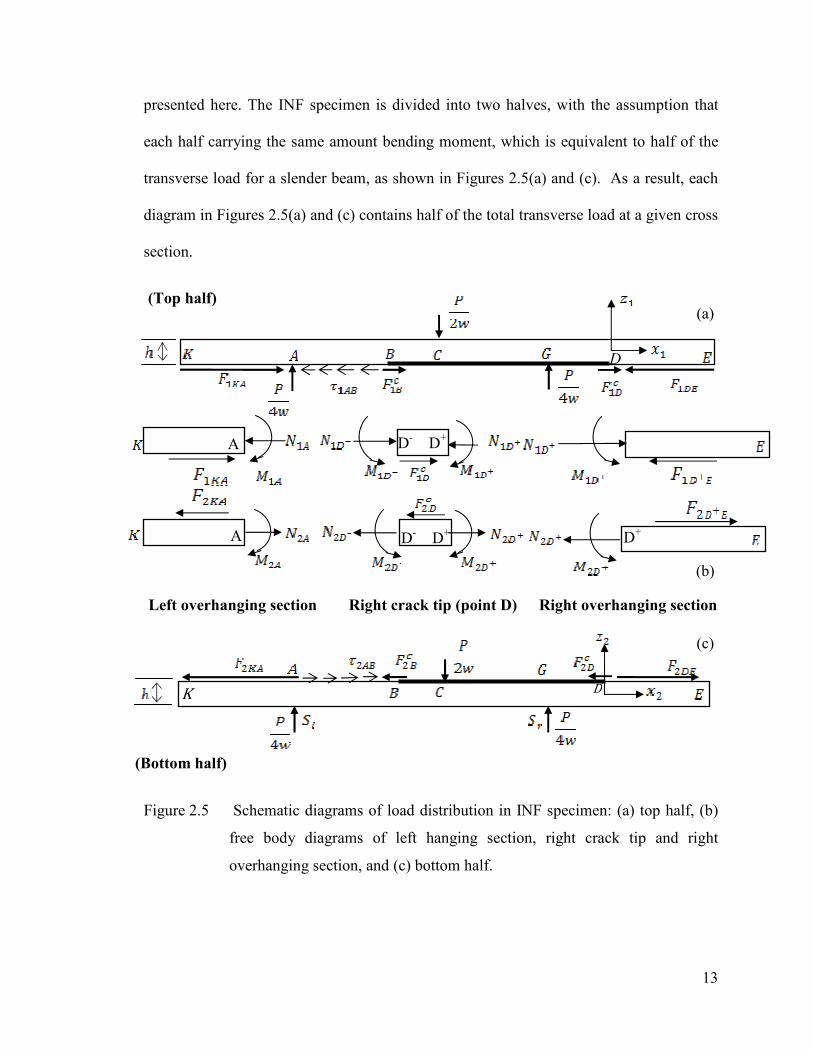
Figure 2.5 Schematic diagrams of load distribution in INF specimen: (a) top half, (b)

free body diagrams of left hanging section, right crack tip and right

overhanging section, and (c) bottom half. ................................................... 13

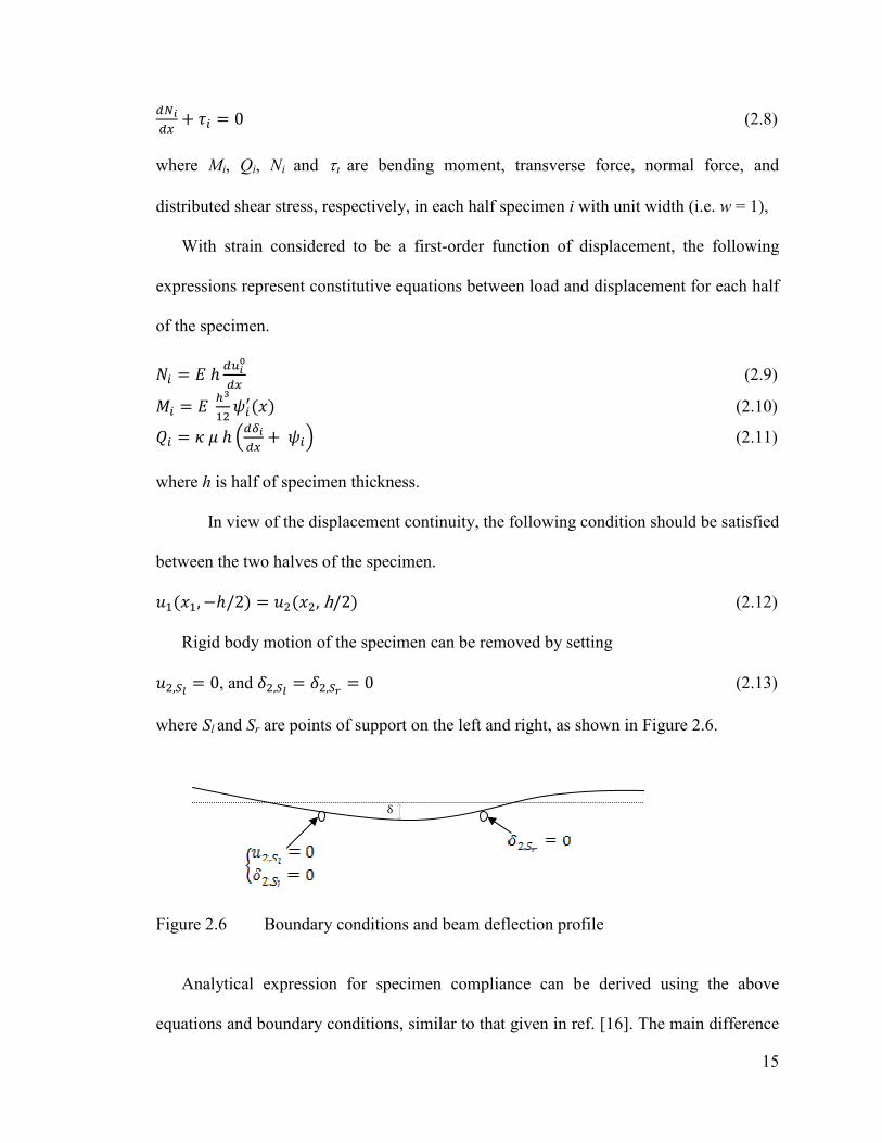
Figure 2.6 Boundary conditions and beam deflection profile. ...................................... 15

Figure 2.7 Schematic diagram of load-displacement curve of the INF test .................. 30

Figure 2.8 Comparison of load-displacement curve generated by analytical solutions in

ref. [16] and current revised solution ........................................................... 32

Figure 3.1 Schematic diagram of the cohesive zone model .......................................... 35

Figure 3.2 Finite-element model of the INF specimen: (a) the overall mesh pattern, (b)

mesh pattern around the inter-laminar region, and (c) an example of the

deflection behavior....................................................................................... 39

Figure 3.3 Load-displacement curve of the INF specimen from FE model. ................. 41

Figure 3.4 Load-displacement curve of the INF specimen from different crack lengths

...................................................................................................................... 43

Figure 3.5 Comparison of load-displacement curve before delamination initiation,

generated by the FE model and analytical solutions ................................... 44

Figure 3.6 Plot of the damage zone length as a function of delamination growth

distance from the right crack tip. ................................................................. 45

Figure 3.7 Depiction of damage development in front of the right crack tip at the

critical load for delamination initiation ....................................................... 46

Figure 3.8 Comparison of load-displacement curve generated by the FE model and

those by the revised analytical solution ...................................................... 48

Figure 3.9 Schematic diagram of elastic-plastic damage material model response ..... 49

Figure 3.10 Schematic diagram of linear isotropic strain-hardening curve ................... 52

Figure 3.11 Schematic diagram of elastic-plastic damage material model with linear

softening ...................................................................................................... 56

Figure 3.12 Schematic diagram of evolution of damage parameter as a function of

dissipated energy ......................................................................................... 58

Figure 3.13 DENT test: (a) specimen configuration, and (b) FE model ........................ 61

Figure 3.14 Stress-Strain curve and development of damage process in DENT test ..... 62

Figure 3.15 Contour plot of equivalent stress in DENT model ...................................... 64

Figure 3.16 Contour plot of damaged elements and crack growth in DENT model ...... 65

Figure 3.17 Load-displacement curve for the DENT test .............................................. 66

Figure 3.18 Schematic diagram of finite element model for DCB specimen with mesh

details at crack tip ....................................................................................... 67

Figure 3.19 FE result of DCB test with the proposed damage material applied to the

interlaminar region: (a) Contour plot of equivalent stress on FE model (b)

contour plot of damage level around the crack tip in the early stage, (c)

contour plot of the damage level around crack tip during the delamination

growth ......................................................................................................... 69

Figure 3.20 FE results of DCB specimen with the proposed damage material property

applied to the entire FE model: (a) Contour plot of equivalent stress, (b)

contour plot of damage parameter around crack tip at the early stage, and (c)

contour plot of the damage parameter around the crack tip during the

delamination growth ................................................................................... 70

Figure 3.21 Finite element model of INF test ................................................................ 71

Figure 3.22 Contour plot of equivalent stress distribution in INF test ........................... 73

Figure 3.23 Deformation profile around crack tip in the INF test ................................. 73

Figure 3.24 Contour plot of damage parameter in the INF specimen ............................ 74

Figure 3.25 Stress-strain curve of INF model from FE simulation ................................ 74

Figure 3.26 Load-displacement curve of INF model from FE solution ......................... 75

List of Tables

Table 2.1 Material property and dimensions of the analytical model of INF specimen

...................................................................................................................... 32

Table 3.1 Dimensions of the FE model of INF specimen. ........................................... 40

Table 3.2 Mechanical properties for top and bottom layers of the INF FE model ...... 40

Table 3.3 Properties of cohesive elements at the interlaminar interface of the FE model

...................................................................................................................... 41

Table 3.4 Geometrical properties used in the DENT model. ....................................... 60

Table 3.5 Material properties of solid elements for DENT FE model ......................... 60

Table 3.6 Dimensions of the FE model of DCB specimen .......................................... 68

Table 3.7 Mechanical properties for top and bottom layers of the DCB FE model used

in this study. ................................................................................................. 68

Table 3.8 Properties of solid elements in the interlaminar region of the DCB FE model

...................................................................................................................... 68

Table 3.9 Properties of solid elements at the interlaminar interface of the INF FE

model............................................................................................................ 71

List of Symbols

a1 crack length, measured from loading pin to furthest crack tip position

a2 crack length, measured from loading pin to nearest crack tip position

ae effective crack length

C compliance

c half ligament length in DENT test

d damage parameter

E Young’ modulus of elasticity

E11 Young’ modulus of in local 1-direction

Eijkl component of the elasticity tensor

c

B

c

B FF 21 , concentrated shear forces at the crack tip point B on top and bottom

halves of a beam respectively

c

D

c

D FF 21 , concentrated shear force at the crack tip point D on top and bottom

halves of a beam respectively

KAKA FF 21 , interlaminar shear force in the overhanging sections KA on top and

bottom halves of a beam respectively

DEDE FF 21 , interlaminar shear force in the overhanging sections DE on top

bottom halves of a beam respectively

G

Ga1

Ga2

energy release rate

energy release rate, associated with crack growth in a1 direction

energy release rate, associated with crack growth in a2 direction

GC critical energy release rate

GIC, GIIC mode I or II critical energy release rate

h beam thickness

k Shear force deformation correction factor in beams

L half span length of INF test

l length of INF specimen

N(x) axial force

P concentrated force

Q shear force

S shear strength

Y tensile strength

T0 original thickness of cohesive zone

U strain energy

U0 Strain energy at damage initiation point

UC Critical strain energy

Ud Dissipated energy during damage process

u displacement vector

u, v, w displacement in the x-, y- or z-direction

u1, u2, u3 displacement in the 1-, 2- or 3-direction

u0 displacement on the neutral axis in the x-direction

w width of a beam

w0 displacement on the neutral axis in the z-direction

α coefficient parameter in damage intitiation criteria

γ, γxy shear strain

δi associated displacements with top and bottom halves of a beam

κ curvature

µ shear modulus

ν Poisson’s ratio

)(xψ beam rotation angle

ijε, ε

strain components and strain tensor

11ε , 22ε , 33ε

normal strains in x-, y- and z-direction

yε

yielding strain

ijσ, σ

Cauchy stress components and stress tensor

11σ , 22σ , 33σ normal stresses in x-, y- and z-direction

yσ yielding stress

τ shear stress

11v , 23v, 13v

Poison’s ratio in orthotropic elastic materials

1

Chapter 1 Introduction

1.1 Background

Composite materials consist of two or more different constituents which are

combined together to create a superior and distinct material. These constituents are

divided into matrix and reinforcement. The reinforcements which are usually small in size

provide strength and rigidity to the new material. The matrix is a lightweight, lower-

strength material which serves as a support to hold the reinforcement together and protect

them from scratches that might generate to damage at a low stress level. It also acts as a

media to transfer load among individual reinforcement. For example, the combination of

fiber glass with polymer creates a unique material called fiber-reinforced polymer (FRP)

and has properties unachievable by each component.

Advanced FRPs have been widely used in aerospace, automotive, construction

and other industries because of their superior mechanical properties such as light weight,

high specific stiffness and strength. However, unexpected excessive loading,

manufacturing defects, shocks and low velocity impact can cause crack initiation and

growth between layers, commonly known as in the interlaminar region. Damage or

separation in the interlaminar region is called delamination which is one of the major

failure modes in FRP to degradation of stiffness, which can lead to loss of effective

2

service lifetime or catastrophic failure of structures [1]. As a result, much of research has

been done in the last two decades, in order to develop accurate analytical and numerical

models that are able to predict delamination development in FRP.

The delamination process commonly involves two stages: initiation and growth.

Delamination initiation is related to the interfacial strength of the material and in many

applications stress-based criteria are used to predict its occurrence [2]. Delamination

growth has been widely investigated based on fracture mechanics. Both analytical and

numerical methods are used to calculate fracture-related parameters such as energy release

rate (G), stress intensity factor (K) or J-integral (J) that serves as a driving force for the

crack growth. Methods such as compliance derivative technique (CDT) [3-4], virtual crack

closure technique (VCCT) [5] or J-integral [6-7] can be used to calculate the energy

release rate (G), and to predict delamination growth by comparing G values to the critical

value (GC) for fracture. However, all of these techniques cannot be directly applied to

prediction of delamination without an initial crack.

Further complication of the finite element implementation arises when progressive

delamination is involved. An alternative solution to avoid the above difficulties is to use

cohesive elements [8-9]. A cohesive damage zone is developed near the crack front and

the crack growth is described by adopting a softening relationship between traction and

relative displacement, with the area under the curve being the critical fracture energy.

Computational issue of cohesive crack model has been extensively investigated by Alfano

et al. [10].

3

1.2 Purpose and scope of research

Purpose of this research is to study stable delamination growth in fiber composites

using analytical and numerical approaches. The analytical approach will be used to

characterize detailed delamination growth in FRP under pure fracture mode II. This

approach will provide essential information on parameters that govern the delamination

growth, such as the extent of damage in front of the crack tip, and the influence of

physical and effective crack lengths in calculating energy release rate, and the speed and

extent of delamination growth. The information, is of great interest to structural engineers,

and can facilitate design of reliable and safe fiber composite structures.

Another essential property of delamination is the fracture toughness which can be

characterized by partitioning the fracture process into three modes: mode I (opening),

mode II (shear) , and mode III (tear). The critical energy release rates under those modes

of fractures can be measured experimentally through appropriate testing methods. In this

study, a critical energy release rate (GIIC) obtained from a previous experimental

investigation on internal-notched flexure (INF) test, is used in the finite-element (FE)

based prediction of delamination onset and growth. It should be noted that the FEM work

described in this study is based on continuum solid element with physically meaningful

criteria for delamination simulation. The use of solid elements will enable us to take into

account all stress components in determining the initiation of delamination.

4

1.3 Structure of thesis

The thesis is divided in two main parts. The first part concentrates on the analytical

approach to predict stable delamination growth in pure mode II fracture, Chapter 2. The

development of an accurate analytical model is a vital tool for predicting delamination

growth in FRP. The analytical expressions for compliance (C) of the INF specimen and its

energy release rate for delamination (G) are derived. The second part is concerned about

finite element simulation of delamination, chapter 3. This chapter provides a basis for

understanding various methods that are conventionally used to simulate delamination in

FRP. Discussion also includes some details of the new proposed damage material model

for delamination simulation.

The last chapter gives a summary of the whole work and identifies problems that

can be considered for the future work.

5

Chapter 2 Analytical Prediction of Stable Delamination

Growth in Internal-Notched Flexure (INF) Test

2.1 Introduction

The delamination process in fiber composites can be characterized by partitioning

the fracture process into three pure modes: the opening (mode I), the in-plane shear (mode

II) and the out-of-plane shear (mode III). The interfacial fracture toughness (GC) of

composites in each mode is different due to the difference in fracture mechanisms and

extensive efforts have been made to devise methods for measuring the critical energy

release rate under mode I and mode II loading with very carefully designed experiments.

This is because firstly GIC and GIIC are the most important parameters to evaluate the

performance of fiber composites’ resistance to fracture and secondly they are essential

input quantities for simulating delamination growth using FEM. The study on

delamination in mode III, on the other hand, has received little attention. Delamination

growth is assumed to take place when the energy release rate reaches a critical value.

Since the change of energy release rate with crack growth can also be used to determine

whether the delamination growth is stable analytical expression for the energy release rate

is very important in the study of delamination propagation.

While the development of mode I delamination test is successful and standardized

[11] using the double cantilever beam (DCB) test, as shown in Figure 2.1(a), there is a

long and winding road to standardize mode II delamination [12]. The four most commonly

6

used test methods to characterize mode II delamination fracture toughness are: end-loaded

split (ELS), end-notch flexure (ENF), including the stabilized version, and four-point bend

ENF (4ENF) tests, as shown in Figures 2.1(b) to 2.1(d). At the time when this thesis is

prepared, none of the above methods has been accepted as the standard due to uncertainty

of crack growth stability during the test. In addition significant data scatter and sometimes

complicated test set-up are also drawbacks for some of those tests. Note that all of those

tests adopt beam-shaped specimen geometries with a pre-crack, of which a brief history is

summarized in ref. [13].

(b)

L

a

2h

P

(a)

P

2h

P

7

Figure 2.1. Schematic diagram of (a) DCB, (b) ELS, (c) ENF, and (d) 4EN

A new test method, named internal-notched-flexure (INF) test, has been reported

in a previous paper [14] to quantify delamination resistance of fibre-reinforced polymers

(FRP) when subjected to transverse loading. Figure 2.2(a) shows the INF test setup that

applies three-point bending to a specimen that contains an embedded insert film at mid-

thickness. Although INF test is very similar to central-notched-flexure (CNF) test [15] as

shown in Figure. 2.2(b), in both specimen design and loading mode, the INF test has the

transverse load applied un-symmetrically with respect to the insert film; while the CNF

test has the transverse load applied symmetrically with respect to the insert film. In

addition, the CNF test requires the insert film to be placed within the two supports; while

the INF test requires one end of the insert film (i.e. point D in Figure. 2.2(a)) to be

outside the span, and the other end (i.e. point B in Figure 2.2(a)) very close to the central

(d)

c

2L

2h

P/2 P/2

a

(c)

2L a

P

2h

8

transverse load. The previous work [14] shows that with a proper choice of a2 value,

delamination growth starts from point D without any crack development from point B.

Figure 2.2 Schematic diagram of (a) INF test methods under three point bending, and (b)

CNF test.

Major advantage of INF test over the other tests is its unconditionally stable

delamination growth. This is due to the continuous force increase during the test, even

after delamination growth has started, as depicted in Figure 2.3. For the other tests, the

load either decreases, such as in end-notched-flexure (ENF) and end-loaded-split (ELS)

tests, or at best, maintains at the same level, such as in (4ENF) test [13]. Figure 2.3

presents a comparison among those test results, which suggests that stability in

delamination growth is in the order of INF > 4ENF > ELS > ENF.

2L 2a

P

2h

C

Sr

2h

2L

a2 a1

L

Delamination crack

/w

Sl

K D B E

A

Interlaminar region

G

(a)

(b)

9

Figure. 2.3. Schematic diagram of load-displacement plots from five mode II

delamination tests [14]

Previous approach [16] to derive the analytical expressions for compliance and energy

release rate of the INF test, as given by Eqns. (2.1-2.3) below, is based on the approach

proposed by Maikuma et al. [15].

��.��

� ��

�� !� ��"��#

(2.1) $��,&'(.��) � * �

��"��#� �+ , 2+ . , . (2.2) $��,&'(.��) � * �

��"��#� �+ � . , 2+�. � 2+�+ (2.3)

where C is the compliance, δ displacement at the central point at which transverse load P

is applied, $�� and $�� the energy release rate for delamination growth from right and left

crack tips, i.e. points D and B in Figure 2.2, respectively, / flexural modulus of the

4ENF

ENF

Load

ELS

Trend of stability

increase of

delamination

growth

Displacement

Critical point for

delamination

growth INF

10

specimen, 0 shear modulus on the plane shown in Figure 2.2, 1 out-of-plane specimen

width, half specimen thickness, . half of the span length, and 2 the correction factor for

shear deformation [17]. Note that in ref. [16], +� and + in the above equations are

defined as physical crack lengths in the specimen.

The approach used in ref. [16] to derive Eqns. (2.1-2.3) has ignored normal force

in the longitudinal direction and bending moment on cross sections at points A and D in

Fig. 2.2. As a result, the overhanging sections, i.e. sections KA and DE, were assumed to

be load-free. This is incorrect for INF specimen, as evident from Figure 2.4 of a finite

element simulation result that shows change in radius of curvature around the right

support, suggesting the existence of load on the cross section around the right crack tip

that is located on the right of right support.

Figure 2.4. Deformation of finite element model of INF specimen

Therefore, this chapter details a revised derivation for specimen compliance and

energy release rate, by considering load in the overhanging sections. The close-form

expression of the compliance is derived based on Timoshenko beam theory and the

energy release rate by the compliance method based on linear elastic fracture mechanics.

Both the compliance method and the Timoshenko beam theory will be briefly reviewed

in this chapter.

11

2.2 Compliance method

The energy release rate (G) for any structural configuration can be determined for

a given load (P) using the compliance method, which links the change in compliance

(dC) due to the change in crack length (da) to the energy release rate, based on linear

elastic fracture mechanics, i.e, (da

dC

w

PG

2

2

= ), where w is the planar crack width.

The key step to use the compliance method is to obtain the expression of C as a

function of a. In the following sections, the compliance expression for the INF specimen

and energy release rate for delamination will be derived based on Timoshenko beam

theory and compliance method, respectively. A brief review of Timoshenko beam theory

is discussed in the following sub-section.

2.2.1 The Timoshenko Beam Theory

The Euler-Bernoulli beam theory neglects shear deformations by assuming that

plane section remains plane and perpendicular to the neutral axis during bending.

However, in reality internal shear stresses develop when a beam is subjected to a

transverse load. These stresses cause sections that are perpendicular to the neutral axis of

the beam to generate transverse shear deformation on the cross-section. Instead of

assuming that the cross-section remains perpendicular to the neutral axis, Timoshenko

beam theory assumes that shear strain is uniform on the cross-section and hence,

increasing the rotation angle of the cross section, as shown by the combination of ψ and γ

in Figure 2.4. The following assumptions are common for both beam theories:

12

Beam deformation is relatively small

1) The beam is long and slender, i.e. the length is much greater than the

width and thickness;

The cross-section of the beam remains plane

2) The beam is made of isotropic, linear elastic material

In the subsequent sections, kinematic and constitutive relationships for the

Timoshenko beam theory are used to derive energy release rate and compliance of the

INF specimen.

Figure 2.4 Deformation of Timoshenko beam.

2.2.2 The Energy Release Rate for INF Test.

Derivation of the energy release rate has the same approach as that described in

ref. [16]. However, instead of ignoring load in the overhanging sections, as adopted for

the work on CNF test [15], the derivation takes into account the load in the overhanging

sections. The assumptions and derivation of the compliance for the INF specimen is

un-deformed deformed

cross-section

ψ

γ

dx

xdw )(

13

presented here. The INF specimen is divided into two halves, with the assumption that

each half carrying the same amount bending moment, which is equivalent to half of the

transverse load for a slender beam, as shown in Figures 2.5(a) and (c). As a result, each

diagram in Figures 2.5(a) and (c) contains half of the total transverse load at a given cross

section.

Figure 2.5 Schematic diagrams of load distribution in INF specimen: (a) top half, (b)

free body diagrams of left hanging section, right crack tip and right

overhanging section, and (c) bottom half.

D

Left overhanging section Right crack tip (point D) Right overhanging section

K

D

(Bottom half)

(Top half)

(c)

(a)

(b)

D-

D+

D

+

D-

D+

A

A

14

Expressions for displacement u in the longitudinal direction and deflection δ in

the transverse direction for the top and bottom halves of the specimen are given below:

56"76, 86# � 569 � 86:6"76# (2.4)

;6 � ;6"76# (2.5)

where subscript i is 1 or 2, standing for top or bottom half of the specimen, respectively;

coordinates xi-zi have the origin located at mid-thickness in each half of the specimen, at a

cross section where the right crack tip < is located, as shown in Figure 2.5; 56"76, 86#, 569,

:6"76#, and ;6"76# are displacement in the xi-direction at point (76, 86), displacement in

the xi-direction at zi = 0 (mid-plane of the half specimen), the angular displacement of the

cross section at xi, and the vertical deflection at xi, respectively.

Loading for each half of the specimen is depicted in Figures 2.5(a) and 2.5(c) for

the top and bottom half of the specimen, respectively, and Figure 2.5(b) gives free-body

diagrams of left and right overhanging sections and the section at right crack tip. Note

that in Figure 2.5, =6>? at point B and =6@? at point D represent a concentrated shear force at

the crack tip, =6AB and =6@� the interlaminar shear force in the overhanging sections KA

and DE, respectively, and τiAB the distributed interlaminar shear stress in section AB.

Each half of the specimen in Figures 2.5(a) and 2.5(c) is divided into four sections

by cross-sections at points A, B, and D. Section BD is further divided into three

subsections by cross sections at points C and G.

Load balance in each section is governed by the following equations [15]:

CDECF , G6 � H6"I/2# � 0 (2.6)

CLECF � 0 (2.7)

15

CMECF � H6 � 0 (2.8)

where Mi, Qi, Ni and τι are bending moment, transverse force, normal force, and

distributed shear stress, respectively, in each half specimen i with unit width (i.e. w = 1),

With strain considered to be a first-order function of displacement, the following

expressions represent constitutive equations between load and displacement for each half

of the specimen.

N6 � / I COEPCF (2.9)

Q6 � / �� :6R"7# (2.10)

G6 � 2 0 I SC�ECF � :6T (2.11)

where h is half of specimen thickness.

In view of the displacement continuity, the following condition should be satisfied

between the two halves of the specimen.

5�"7�, ,I/2# � 5 "7 , h/2# (2.12)

Rigid body motion of the specimen can be removed by setting

5 ,VW � 0, and ; ,VW � ; ,V& � 0 (2.13)

where Sl and Sr are points of support on the left and right, as shown in Figure 2.6.

Figure 2.6 Boundary conditions and beam deflection profile

Analytical expression for specimen compliance can be derived using the above

equations and boundary conditions, similar to that given in ref. [16]. The main difference

δ

16

between the two derivations is the consideration of load in the overhanging sections, i.e.

load in sections KA and DE in Figure 2.2. In the previous derivation [16], because

loading in those sections was ignored cross section at point A was assumed to be load-

free and cross section at point D free from normal force. In the current derivation,

however, shear forces in the interlaminar region of the overhanging sections are

considered. Therefore, normal force and bending moment are considered to exist on cross

sections at points A and D. The key step in the current derivation is to solve for deflection δ from Eqns. (2.6-

2.11) for each half of the specimen, with loading specified in Figures 2.5(a) and 2.5(c)

and displacement continuity for :"76#, ;"76#, and 59"76# across adjacent sections among

KA, AB, BD, and DE. Solutions from each half specimen are then correlated with each

other through displacement continuity between the two halves of the specimen, Eqn.

(2.12), with boundary conditions for bottom half of the specimen given by Eqn. (2.13).

Since boundary conditions in Eqn. (2.13) are for the lower half of the specimen,

linear displacements, ; and 59, and angular displacement of the cross section, :, for the

bottom half of the specimen are solved first. Below are their expressions in terms of x2.

1) Section AB : )()( 2121 aaxLa +−≤≤+−

: B>"7 # � , � �� 7 � 2". � +�#7 � M�Y

�� 7 , � �� "+ � , 3+ . � +� . �

2+�. , .�# , �M�[\ �� "+ � .# � �M�Y

�� "+ � .# � 4+�. (2.14a)

; B>"7 # � �� "7 � � 3". � +�#7 , 2"+� � .#�# , �M�Y

�� "7 , "+� � .# # ,^, �

�� "+ � , 3+ . � +� . � 2+�. , .�# , �M�_ �� "+ � .# � �M�Y

�� ""+ �

.# � 4+�.#` "7 � +� � .# , �� "7 � +� � .# (2.14b)

17

5 B>9 "7 # � �� S �

�� 7 � 2". � +�#7 � 2"+� � .# , N B�7 � 4"+� � .# �S��

T a, � �� "a � , 3a L � +� . � 2a�L , L�# , �M�_

�� "a � .# � �M�Y �� ""a �

.# � 4a�L#dT (2.14c)

2) Section BC: 1221 )( axaa −≤≤+−

: >e"7 # � , � �� 47 � 8". � +�#7 � 3"+� � + #"+� , + � 2.#! �

M�_�� "7 � +� � + # , M�Y

�� "+� � + # , � �� "+ � , 3+ . � +� . � 2+�. , .�# ,

�M�_ �� "+ � .# � �M�Y

�� ""+ � .# � 4+�.# (2.15a)

; >e"7 # � �� "47 � � 12". � +�#7 � 9"+� � + #"+� , + � 2.#7 �

3"+� � + # "3. � +� , 2+ # , 2"+� � .#�# , �M�[\�� "7 � 2"+� � + #7 �

"+� � + # # � �M�Y�� "2"+� � + #7 � "+� � + # � "+� � .# # , ^, �

�� "+ � ,

3+ . � +� . � 2+�. , .�# , �M�[\ �� "+ � .# � �M�Y

�� ""+ � .# � 4+�.#` "7 �. � +�# ,

�� "7 � . � +�# (2.15b)

5 >e9 � �� ^N @\"7 � +� � + # � �

�� ","+� � + #"+� , + � 2.# � 2"+� � .# # �N B",3+� � + , 4.# , �

�� "+ � , 3+ . � +� . � 2+�. , .�#! , �M�[\�� "+ �

.# � �M�Y�� ""+ � .# � 4+�.#` (2.15c)

3) Section CG: )( 121 Laxa +−≤≤−

18

: ei"7 # � � �� "47 � 8",. � +�#7 � 5+� � 3+ , 6+�. , 6+ .# � M�[\

�� "7 �+� � + # , M�Y

�� "+� � + # , � �� "+ � , 3+ . � +� . � 2+�. , .�# ,

�M�[\ �� ""+ � .# # � �M�Y

�� ""+ � .# � 4+�.# (2.16a)

; ei"7 # � �� ",47 � , 12",. � +�#7 , 3"5+� � 3+ , 6+�. , 6+ .#7 ,

7+�� , 9+�+ � 18+�+ . , 6+ � � 9+ . � 3+� . , 6+�. , 2.�# , �M�[\�� "7 �

2"+� � + #7 � "+� � + # # � �M�Y�� "2"+� � + #7 � "+� � + # � "+� � .# # ,

^, � �� "+ � , 3+ . � +� . � 2+�. , .�#! , �M�[\

�� ""+ � .# # � �M�Y �� ""+ �

.# � 4+�.#` "7 � . � +�# , �� ". , 7 , +�# (2.16b)

5 ei9 � �� ^N @\"7 � +� � + # � �

�� ","+� � + #"+� , + � 2.# � 2"+� � .# # �N B",3+� � + , 4.# , �

�� "+ � , 3+ . � +� . � 2+�. , .�#! , �M�[\�� "+ �

.# � �M�Y�� ""+ � .# � 4+�.#` (2.16c)

4) Section GD: 0)( 21 ≤≤+− xLa

: i@"7 # � �M�[\ �� "4.7 , "+ , .# � 4.+�# � �

�� "3+ . , 3+ . , 3.� , + �# ��M�Y

�� ""+ , .# # (2.17a) ; i@"7 # � �M�[\

�� ,2.7 � "+ , .# 7 , 4.+�7 � 2.",+� � .# , "+ ,.# ",+� � .# � 4.+�",+� � .#! , �

�� "3+ . , 3+ . , 3.� , + �#7 ,"3+ . , 3+ . , 3.� , + �#",+� � .#! , �M�Y

�� "+ , .# 7 , "+ , .# ",+� �.#! (2.17b)

19

5 i@9 � �� SN @\"7 � +� � + # � �

�� ,"+� � + #"+� , + � 2.# � 2"+� � .# �N B",3+� � + , 4.# , �

�� "+ � , 3+ . � +� . � 2+�. , .�#! , �M�[\�� "+ �

.# � �M�Y�� "+ � .# � 4+�.T (2.17c)

5) Section DE: rlx ≤≤ 20 , where rl is length of un-delaminated region in the right

overhanging section of the specimen

: @�"7 # � , M�[m�� SF�

n& , 7 T � �M�[\ �� ","+ , .# � 4.+�# � �

�� "3+ . ,3+ . , 3.� , + �# � �M�Y

�� "+ , .# (2.18a)

; @�"7 # � , S, M�[m�� S F�

n& , � 7 T � ^�M�[\

�� ","+ , .# � 4.+�# � � �� "3+ . ,

3+ . , 3.� , + �# � �M�Y �� ""+ , .# #` 7 T � �M�[\

�� 2.",+� � .# , "+ ,.# ",+� � .# � 4.+�",+� � .#! , �

�� ,"3+ . , 3+ . , 3.� , + �#",+� �.#! , �M�Y

�� ,"+ , .# ",+� � .#! (2.18b)

5 @�9 "7 # � �� oN @m S F��

n& , 7T � N @\"+� � + # � � �� ","+� � + #"2. � +� , + # �

2"+� � .# # � N B",3+� , + , 2.# , � �� "+ � , 3+ . � +� . � 2+�. , .�# ,

�M�[\�� "+ � .# � �M�Y

�� ""+ � .# � 4+�.#p (2.18c)

In a similar manner, expressions for deflection, ;"7�#, angular displacement of the cross-

section, :"7�#, and displacement along neutral axis, 59"7�#, of various sections in the

upper half of the specimen are:

1) Section AB: )()( 2111 aaxLa +−≤≤+−

20

:�B>"7�# � , � �� "7� � 2". � +�#7�# � M�Y

�� 7� , � �� "+ � , 3+ . � +� . �

2+�. , .�# , �M�[\ �� "+ � .# � �M�Y

�� ""+ � .# � 4+�.# (2.19a)

;�B>"7�# � �� "7�� 3". � +�#7� , 2"+� � .#�# , �M�Y

�� "7� , "+� � .# # ,^, �

�� "+ � , 3+ . � +� . � 2+�. , .�# , �M�[\ �� "+ � .# � �M�Y

�� ""+ �

.# � 4+�.#` "7� � +� � .# , �� "7� � +� � .# (2.19b)

5�B>9 "7�# � �� ^ �

�� "7 � 2". � +�#7 � 4"+� � .# # � N�B7 , 2N�B"+� � .# ,6N B"+� � .# � , *

�� "+ � , 3+ . � +� . � 2+�. , .�# , *M�[\�� "+ � .# �

*M�Y�� ""+ � .# � 4+�.#`(19c)

2) Section BC: 1121 )( axaa −≤≤+−

:�>e"7�# � , � �� 47� � 8". � +�#7� � 3"+� � + #"+� , + � 2.#! � M�_

�� "7� �+� � + # , M�Y

�� "+� � + # , � �� "+ � , 3+ . � +� . � 2+�. , .�# ,

�M�_ �� "+ � .# � �M�Y

�� ""+ � .# � 4+�.# (2.20a)

;�>e"7�# � �� "47�� 12". � +�#7� � 9"+� � + #"+� , + � 2.#7� � 3"+� �

+ # "3. � +� , 2+ # , 2"+� � .#�# , �M�[\�� "7� � 2"+� � + #7� � "+� � + # # �

�M�Y�� "2"+� � + #7� � "+� � + # � "+� � .# # , ^, �

�� "+ � , 3+ . � +� . �

2+�. , .�# , �M�[\ �� "+ � .# � �M�Y

�� ""+ � .# � 4+�.#` "7� � . � +�# ,

�� "7� � . � +�# (2.20b)

21

5�>e9 "7�# � �� ^,N�@\"7� � +� � + # � �

�� ""+ , .# � 3"+� � .# # , N�B"4. �3+� , + # , 6N�B"+� � .# , *

�� "+ � , 3+ . � +� . � 2+�. , .�# ,*M�[\

�� "+ � .# � *M�Y�� ""+ � .# � 4+�.#` (2.20c)

3) Section CG: )( 111 Laxa +−≤≤−

:�ei"7�# � � �� "47� � 8",. � +�#7� � 5+� � 3+ , 6+�. , 6+ .# � M�[\

�� "7� �+� � + # , M�Y

�� "+� � + # , � �� "+ � , 3+ . � +� . � 2+�. , .�# ,

�M�[\ �� ""+ � .# # � �M�Y

�� ""+ � .# � 4+�.# (2.21a)

;�ei"7�# � �� ",47�� , 12",. � +�#7� , 3"5+� � 3+ , 6+�. , 6+ .#7� ,

7+�� , 9+�+ � 18+�+ . , 6+ � � 9+ . � 3+� . , 6+�. , 2.�# , �M�[\�� "7� �

2"+� � + #7� � "+� � + # # � �M�Y�� "2"+� � + #7� � "+� � + # � "+� � .# # ,

^, � �� "+ � , 3+ . � +� . � 2+�. , .�#! , �M�[\

�� ""+ � .# # � �M�Y �� ""+ �

.# � 4+�.#` "7� � . � +�# , �� ". , 7� , +�# (2.21b)

5�ei9 "7�# � �� ^,N�@\"7� � +� � + # � �

�� ""+ , .# � 3"+� � .# # , N�B"4. �3+� , + # , 6N�B"+� � .# , *

�� "+ � , 3+ . � +� . � 2+�. , .�# ,*M�[\

�� "+ � .# � *M�Y�� ""+ � .# � 4+�.#` (2.21c)

4) Section GD: 0)( 11 ≤≤+− xLa ,

22

:�i@"7�# � M�[\�� "7� � +� � + # � �

�� "+� � 3+ � 2+�. , 6+ . , 4. # ,M�Y�� "+� � + # , �

�� "+ � , 3+ . � +� . � 2+�. , .�# , �M�[\ �� "+ � .# �

�M�Y �� ""+ � .# � 4+�.# (2.22a)

;�i@"7�# � �M�[\ �� ,2.7� � "+ , .# 7� , 4.+�7� � 2.",+� � .# , "+ ,

.# ",+� � .# � 4.+�",+� � .#! , � �� "3+ . , 3+ . , 3.� , + �#7� ,

"3+ . , 3+ . , 3.� , + �#",+� � .#! , �M�Y �� "+ , .# 7� , "+ , .# ",+� �

.#! (2.22b)

5�i@9 "7�# � �� ^,N�@\"7� � +� � + # , �

�� "+� � + #"2. � +� , + #! ��

�� "+� � .# � N�B",3+� , + , 2.# , 6N B"+� � .# , * �� "+ � , 3+ . �

+� . � 2+�. , .�# , *M�[\�� "+ � .# � *M�Y

�� ""+ � .# � 4+�.#` (2.22c)

5) Section DE: rlx ≤≤ 10 , where rl length of undelaminated region in the right

overhanging section of the specimen

:�@m�"7�# � , M�[m�� S F��

n& , 7�T � �M�[\ �� ","+ , .# � 4.+�# � �

�� "3+ . ,3+ . , 3.� , + �# � �M�Y

�� ""+ , .# # (2.23a)

;�@�"7�# � , S, M�[m�� S F��

n& , � 7� T � ^�M�[m

�� ","+ , .# � 4.+�# � � �� "3+ . ,

3+ . , 3.� , + �# � �M�Y �� ""+ , .# #` 7�T � �M�[\

�� 2.",+� � .# , "+ ,.# ",+� � .# � 4.+�",+� � .#! , �

�� ,"3+ . , 3+ . , 3.� , + �#",+� �.#! , �M�Y

�� ,"+ , .# ",+� � .#! (2.23b)

23

5�@�9 "7�# � �� oN�@m S F��

n& , 7�T , N�@"+� � + # � � �� ""+ , .# � 3"+� � .# # ,

N�B"4. � 3+� , + # , 6N B"+� � .# � S�� T ^

�� ,3"+ � , 3+ . � +� . �

2+�. , .�#! , �M�[\ �� "+ � .# � �M�Y

�� ""+ � .# � 4+�.#`p (2.23c)

On cross sections at points q,< and E in Figure 2.2, expressions for 59and : for each

half of the specimen are:

(i) In the top half of the specimen:

5�B>9 ",+� , + # � �� ^ �

�� ""+ , .# � 3"+� � .# # � N�B",3+� , + , 2.# ,6N�B"+� � .# � , *

�� "+ � , 3+ . � +� . � 2+�. , .�# , *M�[\�� "+ � .# �

*M�Y�� ""+ � .# � 4+�.#` (2.24a)

5�i@9 "0# � �� ^,N�@\"+� � + # , �

�� "+� � + #"2. � +� , + #! � � �� "+� � .# ,

N�B"3+� � + � 2.# , 6N B"+� � .# , * �� "+ � , 3+ . � +� . � 2+�. , .�# ,

*M�[\�� "+ � .# � *M�Y

�� ""+ � .# � 4+�.#` (2.24b)

5�@�9 "r�# � �� oN�@m Sn&�

n& , r�T , N�@\"+� � + # � � �� ""+ , .# � 3"+� � .# # ,

N�B"4. � 3+� , + # , 6N�B"+� � .# � � �� ,3"+ � , 3+ . � +� . � 2+�. ,

.�#! , *M�[\�� ""+ � .# # � *M�Y

�� ""+ � .# � 4+�.#p (2.24c)

:�B>",+� , + # � � �� "+� � + #"2. � +� , + #! , M�Y

�� "+� � + # , � �� "+ � ,

3+ . � +� . � 2+�. , .�# , �M�[\ �� "+ � .# � �M�Y

�� ""+ � .# � 4+�.# (2.24d)

24

:�i@"0# � M�[\�� "+� � + # � �

�� "+� � 3+ � 2+�. , 6+ . , 4. # , M�Y�� "+� �

+ # , � �� "+ � , 3+ . � +� . � 2+�. , .�#! , �M�[\

�� ""+ � .# # ��M�Y

�� ""+ � .# � 4+�.# (2.24e)

:�@�"r�# � �n&M�[m�� M�[\

�� ","+ , .# � 4.+�# � � �� "3+ . , 3+ . , 3.� ,

+ �# � �M�Y �� "+ , .# (2.24f)

(ii) In the bottom half of the specimen

5 B>9 ",+� , + # � �� ^ �

�� ","+� � + #"+� , + � 2.# � 2"+� � .# # �N B�",3+� � + , 4.#! , �

�� "+ � , 3+ . � +� . � 2+�. , .�# , �M�[\�� "+ �

.# � �M�Y � ""+ � .# � 4+�.#` (2.25a)

5 i@9 "0# � �� ^N @\"+� � + # � �

�� ","+� � + #"+� , + � 2.# � 2"+� � .# # �N B",3+� � + , 4.# , �

�� "+ � , 3+ . � +� . � 2+�. , .�# , �M�[\�� "+ �

.# � �M�Y�� ""+ � .# � 4+�.#` (2.25b)

5 @�9 "r�# � �� ^, n& M�[m

� N @\"+� � + # � � �� ","+� � + #"2. � +� , + # �

2"+� � .# # � N B",3+� , + , 2.# , � �� "+ � , 3+ . � +� . � 2+�. , .�# ,

�M�[\�� "+ � .# � �M�Y

�� ""+ � .# � 4+�.#` (2.25c)

: B>",+� , + # � � �� "+� � + #"+� , + � 2.# , M�Y

�� "+� � + # , � �� "+ � ,

3+ . � +� . � 2+�. , .�# , �M�[\ �� "+ � .# � �M�Y

�� ""+ � .# � 4+�.# (2.25d)

25

: i@"0# � M�[\�� "+� � + # � �

�� "+� � 3+ � 2+�. , 6+ . , 4. # , M�Y�� "+� �

+ # , � �� "+ � , 3+ . � +� . � 2+�. , .�# , �M�[\

�� "+ � .# � �M�Y �� ""+ �

.# � 4+�.# (2.25e)

: @�"r�# � �n& M�[m�� M�[\

�� ","+ , .# � 4.+�# � � �� "3+ . , 3+ . , 3.� ,

+ �# � �M�Y �� "+ , .# (2.25f)

Boundary conditions selected here are given as in the following expressions. The first

two are to set displacement ui at the left and right crack tips to be the same between the

top and bottom halves of the specimen, which is the relaxed version of the assumption

made by Maikumar et al. [15]. The third boundary condition, in view that the crack only

grows from the right crack tip, is to set displacement ui at point A, the interlaminar point

above the left support, to be the same between the top and bottom halves of the specimen.

5�",+� , + , ,I/2# � 5 ",+� , + , I/2# (2.26a)

5�"0, ,I/2# � 5 "0, I/2# (2.26b)

5�",. , +�, ,I/2# � 5 ",. , +�, I/2# (2.26c)

where expressions for 5� and 5 are

5�",+� , + , ,I/2# � 5�B>9 ",+� , + # , S� T :1sq",+� , + # (2.27a)

5 ",+� , + , I/2# � 5 B>9 ",+� , + # � S� T :2sq",+� , + # (2.27b)

5�"0, ,I/2# � 5�i@9 "0# , S� T :�i@"0# (2.27c)

5 "0, I/2# � 5 i@9 "0# � S� T : i@"0# (2.27d)

5�",. , +�, ,I/2# � 5�B>9 ",. , +�# , S� T :�B>",. , +�# (2.27e)

26

5 ",. , + , I/2# � 5 B>9 ",. , + # � S� T : B>",. , + # (2.27f)

Based on expressions given in Eqns. (2.24-2.25), the above boundary conditions can

be used to solve forN6B, N6@\and N6@m. Note that N�B � N B, N�@\ � N @\ and N�@m � N @m due to symmetry of the loading conditions, as shown by free body diagrams in

Figure 2.5(b). This yields

N6B � , � � �� ". , + # (2.28a)

N6@\ � , � ��"��# "+ , 2+ . , . # (2.28b)

N6@m � , � � ��n& "3.+� � + . , 3+ +� , 2+ � 3. # (2.28c)

Once the above normal forces are determined, expressions for the concentrated

forces, = >? and = @e can be expressed below, based on free body diagrams of the left and

right crack tips. Note that the free body diagram for the right crack tip in Figure 2.5(b)

can also represent the free body diagram for the left crack tip, by replacing “D” in the

diagram by “B.” Expressions for the concentrated forces, = >? and = @? , are

= >? � � ��"��# ^+ � 2+�+ , 2+�. � . , �

"+� � + #". , + #` (2.29a)

= @? � � ��"��# o+ , 2+ . , . , "��#

n& "3.+� � + . , 3+ +� , 2+ � 3. #p

(2.29b)

If shear force in the interlaminar region of the overhanging section is ignored, the

expressions in Eqns. (2.29a) and (2.29b) are reduced to

= >? � � ��"��# "+ � 2+�+ , 2+�. � . # (2.30a)

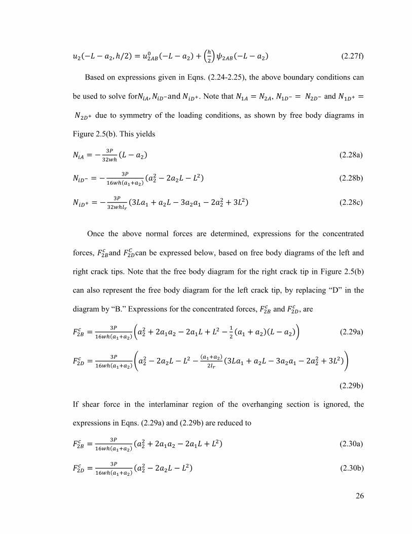
= @? � � ��"��# "+ , 2+ . , . # (2.30b)

27

By substituting Eqns. (2.28a) and (2.28b) into Eqn. (2.21b), the center deflection of the

specimen,;�ei",+�#, is:

;�ei",+�# � , �� , �

�� , � �� "+ � , 3+ . � 3+ . � .�# � *

� ��"��# "+ ,2+ . , . # � *

�� "+ , .#� (2.31)

Hence, compliance for the specimen � is:

� � � ^��_v"\w�#� x ` � ��

�� !

� ��"��# �*

�� ". , + #� (2.32)

In Eqn. (2.32), the fourth term on the right-hand side is due to the consideration of

interlaminar shear force in the overhanging section. If ignored, the expression for C is

reduced to Eqn. (2.1).

It should be noted that a unidirectional fiber composite beam is transversely isotropic,

not isotropic as assumed for the beam theory used here. However, since the deformation

is considered to be in the plane-strain condition with modulus in the axial direction

affecting the deformation, the beam theory is still applicable as long as the material

constants E and µ represent flexural modulus in the longitudinal direction and shear

modulus on the longitudinal-thickness plane, respectively. For example, in the case that

the local 1-direction of the material is along the longitudinal direction, the material

constants E and µ in Eqn. (2.32) represent E11 and µ12, respectively.

Based on the compliance method discussed in section 2.2.1 [18], the energy

release rate G for delamination growth in directions +6 is

$�E � � �

yey�E (2.33)

That is,

28

$�� * ��"��#� �+ , 2+ . , . (2.34a)

$�� * ��"��#� a"+ � 2+�+ , 2+�. � . # , �

"+� � + # ". , + # d (2.34b)

Note that if the interlaminar shear load in the overhanging sections were ignored, the

expressions for Gai would then be reduced to Eqns. (2.2) and (2.3) that were reported in

ref. [16].

Now the total energy release rate G for crack growth from the two crack fronts

can be expressed as a function of $�� and $�� , by incorporating fraction of the

delamination growth length in the two directions, i.e.,

$ � z��z��z�� $�� z��

z��z�� $�� (2.35)

For delamination growth only in a1-direction, $�� has to be greater than $�� ,

which can be met by enforcing $��> $�� for the initial values of a1 and a2. In addition, a1

should be longer than L. Therefore, the initial values for a1 and a2 should meet the

following condition [16]:

LaL

aLaL

2

21 −

+≤≤ (2.36)

When the above condition is met,

$ � $�� * ��"��#� �+ , 2+ . , . (2.37)

Eqn. (2.36) also suggests that a limit exists for the growth of a1 before delamination

growth starts in a2-direction. Therefore, dimensions of the INF specimen should be

designed to ensure that the specimen provides sufficient growth in a1-direction before the

growth in a2-direction starts, for ease of establishing the resistance curve for

delamination.

29

2.3 Prediction of Load-Displacement Curve for INF test

In the condition that delamination grows in +� direction only, Eqn. (2.37) can be

used to construct load-displacement curve for INF test provided that critical energy

release rate GC is constant during the delamination growth. In this case, load P can be

expressed as:

{ � �"��#|��i_�� ! (2.38)

The corresponding expression for the displacement ; is

; � |i_��*}��~�}�� 9~�}��}��~�~�}��~�~��}�� ~�~��!� √��}�� ~�}��! � *|i_"~��~�#"��~�#�

�√��}�� ~�}��!

(2.39)

If the interlaminar shear forces in the overhanging sections are ignored, the displacement

δ becomes:

; � |i_��*}��~�}�� 9~�}��}��~�~�}��~�~��}�� ~�~��!� √��}�� ~�}��! (2.40)

Note that Eqn. (2.40) is still applicable to the case that the interlaminar shear forces

in the overhanging sections are ignored.

The prediction of the above analytical expressions for the load-displacement curve is

schematically demonstrated in Figure. 2.7, showing the change with respect to the

increase of +� and $e.

30

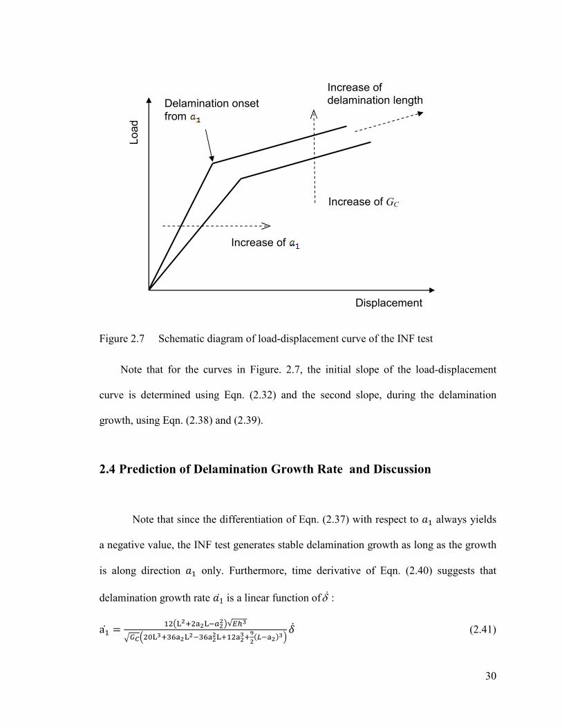
Figure 2.7 Schematic diagram of load-displacement curve of the INF test

Note that for the curves in Figure. 2.7, the initial slope of the load-displacement

curve is determined using Eqn. (2.32) and the second slope, during the delamination

growth, using Eqn. (2.38) and (2.39).

2.4 Prediction of Delamination Growth Rate and Discussion

Note that since the differentiation of Eqn. (2.37) with respect to +� always yields

a negative value, the INF test generates stable delamination growth as long as the growth

is along direction +� only. Furthermore, time derivative of Eqn. (2.40) suggests that

delamination growth rate +1� is a linear function ofδ& :

a�� }�� ~�}��!√��|i_S 9}��~�}��~��}�� ~��

�"��~�#�T ;� (2.41)

Delamination onset from

Increase of delamination length

Displacement

Increase of GC

Lo

ad

Increase of

31

That is, with a2 and GC being constant, the INF test can be conducted at different

crosshead speeds, without concerns about the stability of delamination growth. This is an

advantage of INF test, especially for the study of the influence of crack growth rate on

the delamination development. Therefore, the test can be used to study influence of

loading rate on the delamination resistance.

As evident in Figure 2.8, the predictions of delamination growth using the analytical

solutions in ref. [16] and the current revised solutions are demonstrated using the load-

displacement curve with respect to a constant physical crack length +� and $e. It should also be noted that these curves are constructed based on the assumption of

stress-free fracture surfaces that do not impose any barrier for the delamination growth.

Schuecker and Davidson [19] utilized the 4ENF test specimen to analyze the effect of

friction on G for pure mode II using finite element analysis and found that it only

increases the $��evalue by no more than 2%. Therefore, in this study, the effect of friction

on $e is neglected for simplicity and with this assumption, according to Eqn. (2.38) and

(2.39), the slope of the {-; curve during the delamination growth should be independent

of the $evalue.

It should be pointed out that the analytical expression in ref. [16] and current version

have the same expressions for energy release rate $��but different for $�� .The critical

energy release rate Gc = 3190 J/m2

in Figure 2.8, is computed using eq. (2.37) with the

specimen data in Table 2.1.

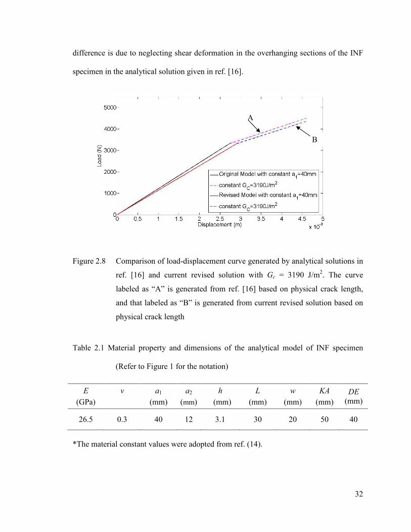
Comparison of the difference in percentage for the compliance and displacement for

specimen dimensions given in Table 2.1 are 11.7% and 7.2% respectively. This

32

difference is due to neglecting shear deformation in the overhanging sections of the INF

specimen in the analytical solution given in ref. [16].

Figure 2.8 Comparison of load-displacement curve generated by analytical solutions in

ref. [16] and current revised solution with Gc = 3190 J/m2. The curve

labeled as “A” is generated from ref. [16] based on physical crack length,

and that labeled as “B” is generated from current revised solution based on

physical crack length

Table 2.1 Material property and dimensions of the analytical model of INF specimen

(Refer to Figure 1 for the notation)

*The material constant values were adopted from ref. (14).

E

(GPa)

v

a1

(mm)

a2

(mm)

h

(mm)

L

(mm)

w

(mm)

KA

(mm)

DE

(mm)

26.5 0.3 40 12 3.1 30 20 50 40

B

A

33

2.5 Concluding remarks

In this chapter, a revised analytical model of the INF specimen to

characterize mode II fracture toughness of fiber composites is developed. The model is base on Timoshenko beam theory and considers the effect of interlaminar shear in the overhanging section on the compliance and global deformation of the specimen. Explicit expressions for compliance and displacement derived here indicated that the interlaminar shear stress variation has a significant contribution and

hence must be incorporated in the analytical solution. The drawback of the analytical

approach is that its application is generally restricted to problems that involve simple

geometry, loads or boundary conditions with linear elastic systems.

34

Chapter 3 Finite Element Simulation of Stable

Delamination Development

3.1 Introduction

The study of delamination process commonly involves two stages: initiation and

growth. Delamination initiation is related to the inter-laminar strength of the material and

in many applications stress-based criteria have been used to predict it. Delamination

growth has been widely investigated using the theory of fracture mechanics through

analytical and numerical approaches. The finite element method can be used to calculate

fracture parameters such as energy release rate (G), stress intensity factor (K) or J-integral

(J) that serves as a driving force for crack growth. Techniques such as the compliance

derivative technique (CDT), virtual crack closure technique(VCCT) or J-integral can be

used to calculate energy release rate (G), and predict delamination growth by comparing G

values to the critical value (GC) which is the material’s resistance to fracture. However, all

these techniques can’t be directly applied to predict delamination without an initial crack

and further complication of the finite element implementation of those methods arises

when progressive delamination is involved.

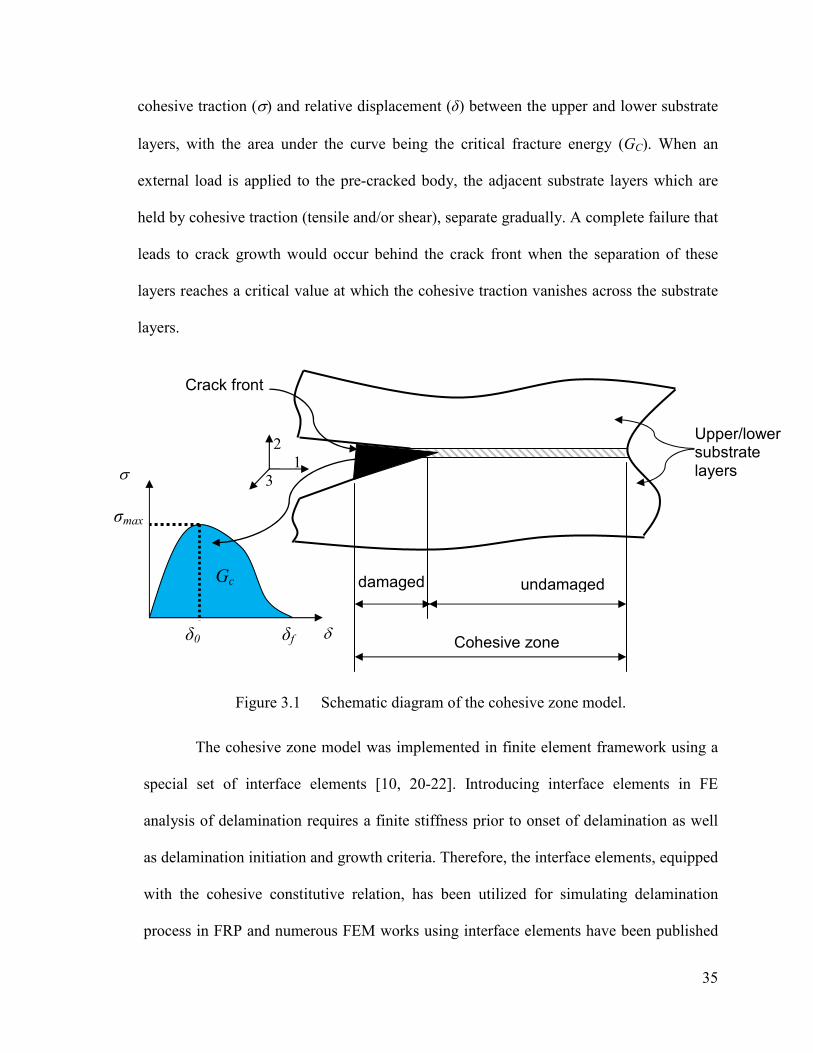
An alternative solution to avoid the above difficulties is to model delamination

development using cohesive zone model. As shown in Figure 3.1, in this approach, a

cohesive damage zone is developed near the crack front. Material behavior in the cohesive

zone follows a cohesive constitutive law which adopts a softening relationship between

35

cohesive traction (σ) and relative displacement (δ) between the upper and lower substrate

layers, with the area under the curve being the critical fracture energy (GC). When an

external load is applied to the pre-cracked body, the adjacent substrate layers which are

held by cohesive traction (tensile and/or shear), separate gradually. A complete failure that

leads to crack growth would occur behind the crack front when the separation of these

layers reaches a critical value at which the cohesive traction vanishes across the substrate

layers.

Figure 3.1 Schematic diagram of the cohesive zone model.

The cohesive zone model was implemented in finite element framework using a

special set of interface elements [10, 20-22]. Introducing interface elements in FE

analysis of delamination requires a finite stiffness prior to onset of delamination as well

as delamination initiation and growth criteria. Therefore, the interface elements, equipped

with the cohesive constitutive relation, has been utilized for simulating delamination

process in FRP and numerous FEM works using interface elements have been published

2

1

3

Cohesive zone

damaged undamaged

Upper/lower substrate layers σ

δ

Gc

δ0 δf

σmax

Crack front

36

in the literature [23-25] . However, like the other numerical techniques mentioned earlier,

application of this method is limited to prediction of delamination with an initial crack.

Disadvantage of the interface elements and other methods such as the use of spring

elements to implement the cohesive zone model in FEM are well documented [26].

To overcome the limitation of interface elements, Fan et al. [27] introduced a new

approach to implement the cohesive zone model in FEM using solid elements with

cohesive damage material property. Unlike the interface elements where the delamination

initiation criterion is described by a combination of only tensile and shear traction

components, solid elements have all stress components so that multi-axial-stress-based

damage initiation criteria can be adopted. Furthermore, the constitutive law of the

cohesive damage material model assumes a linear-elastic response prior to the onset of

delamination and the linear softening law for damage evolution, based on the concept of

linear fracture mechanics.

However, in many practical applications, there could be a substantial plastic

deformation in the resin rich region where delamination growth should not be based on

linear elastic damage material model. In this regard, there are many damage material

models in the literature to simulate the delamination development using cohesive

elements. For example, in ref. [33] elastic-plastic cohesive zone model is used to study

facture behavior of metal-matrix composites under elastoplastic deformation. In ref. [34]

inter-laminar delamination process was modeled using 3D elastic-plastic finite element

model in ABAQUS. However, these damage models were implemented using cohesive

elements with a traction-separation constitutive relation, which has some intrinsic

limitations. Therefore this study investigates delamination growth undergoing plastic

37

deformation in the inter-laminar region using solid elements with damage material

property. The formulation of plastic deformation of the material in the inter-laminar

region is based on von Mises criteria. The simulation of delamination growth involves

gradual degradation of material stiffness along the inter-laminar region ahead of the crack

tip. The constitutive equation of the material in the inter-laminar region is described by

elastic-plastic damage material model. Compared to the cohesive elements, this damage

material model has the advantage of being able to adopt a multi-axial-stresses-based

delamination initiation criterion. Besides, the proposed elasto-plasitc damage material

model uses strain energy to define the damage status.

This chapter is organized as follows. Section 3.2 provides the FE analysis of

delamination growth using cohesive elements, tailored for application to INF test. The FE

solution will be used to verify the revised analytical expressions for compliance of the

INF specimen and its energy release rate for delamination derived in chapter 2. Based on

the FE model, damage evolvement in front of the crack tip is investigated, and the use of

an effective crack length to replace physical crack length for calculation of G is

discussed. Section 3.3 summarizes the new proposed elastic-plastic damage material

model. Section 3.4 describes the finite element simulation of delamination growth using

solid elements with the elastic-plastic damage material model properties tailored for an

application to double-edge-notched tensile (DENT) specimen, double-cantilever-beam

(DCB) specimen and internal-notched-flexure (INF) test and. Finally, section 3.5,

presents some concluding remarks.

38

3.2 Cohesive Elements

3.2.1 Finite Element Model of INF Specimen using Cohesive Elements

Delamination growth in the INF model shown in Figure 2.2 is studied using

cohesive elements to validate the analytical expressions for compliance and energy release

rate derived in chapter 2. A two- dimensional FE model of INF specimen was created

using a commercial code ABAQUS/Standard v6.9 [28]. Overall length of the model is 160

mm, of which dimensions for each section are listed in Table 2.1. The model has three

layers. The top and bottom layers represent substrates of the composite material,

consisting of 4-node, plane-strain elements (CPE4I) with incompatible mode of

orthotropic elastic properties. The middle layer represents the interlaminar region which

includes initial crack lengths of 40 mm for a1 and 12 mm for a2. A frictionless, small

sliding contact is defined between the crack surfaces to avoid penetration. The un-cracked

region in the middle layer consists of cohesive elements (COH2D4) that are connected

with the top and bottom layers using mesh-tie constraint. Dimensions of the cohesive

elements are 0.02 × 0.02 mm; while those in the top layers are 0.25 × 0.25 mm and in the

bottom layer 0.5 × 0.5 mm. Totally, 4596 elements were used to model the top and bottom

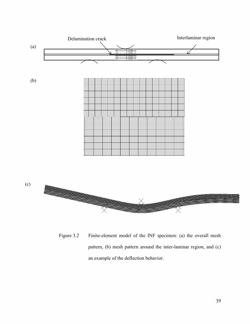
layers, and 2160 elements for the middle layer. Figure 3.2(a) shows the overall mesh

pattern of the model, and Figure 3.2(b) the detailed mesh pattern around the interlaminar

region. An example of the deflection behavior during the delamination growth is given in

Figure 3.2(c).

39

Figure 3.2 Finite-element model of the INF specimen: (a) the overall mesh

pattern, (b) mesh pattern around the inter-laminar region, and (c)

an example of the deflection behavior.

(c)

(b)

Interlaminar region Delamination crack

(a)

40

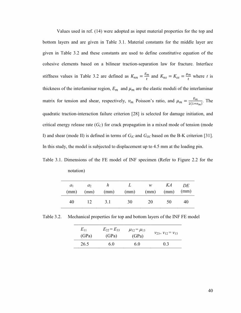
Values used in ref. (14) were adopted as input material properties for the top and

bottom layers and are given in Table 3.1. Material constants for the middle layer are

given in Table 3.2 and these constants are used to define constitutive equation of the

cohesive elements based on a bilinear traction-separation law for fracture. Interface

stiffness values in Table 3.2 are defined as �� and ��

� where t is

thickness of the interlaminar region, / and 0 are the elastic moduli of the interlaminar

matrix for tension and shear, respectively, ¡ Poisson’s ratio, and 0 � �� "��¢�#. The

quadratic traction-interaction failure criterion [28] is selected for damage initiation, and

critical energy release rate (GC) for crack propagation in a mixed mode of tension (mode

I) and shear (mode II) is defined in terms of GIC and GIIC based on the B-K criterion [31].

In this study, the model is subjected to displacement up to 4.5 mm at the loading pin.

Table 3.1. Dimensions of the FE model of INF specimen (Refer to Figure 2.2 for the

notation)

Table 3.2. Mechanical properties for top and bottom layers of the INF FE model

E11

(GPa)

E22 = E33

(GPa)

µ12 = µ13

(GPa) v23= v12 = v13

26.5 6.0 6.0 0.3

a1

(mm)

a2

(mm)

h

(mm)

L

(mm)

w

(mm)

KA

(mm)

DE

(mm)

40 12 3.1 30 20 50 40

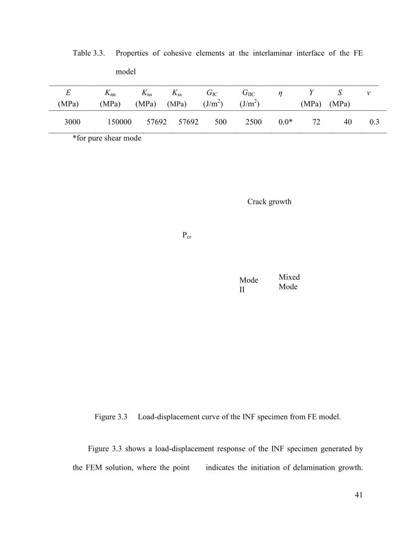
Table 3.3. Properties of cohesive elements at the interlaminar interface of the FE

model

E

(MPa)

Knn

(MPa)

Kns

(MPa)

3000 150000 57692

*for pure shear mode

Figure 3.3 Load

Figure 3.3 shows a load

the FEM solution, where the point

of cohesive elements at the interlaminar interface of the FE

Pa)

Kss

(MPa)

GIC

(J/m2)

GIIC

(J/m2)

η

(MPa)

57692 57692 500 2500 0.0*

oad-displacement curve of the INF specimen from FE model

Figure 3.3 shows a load-displacement response of the INF specimen generated by

the FEM solution, where the point indicates the initiation of delamination growth.

Crack growth

Mixed

Mode Mode

II

Pcr

41

of cohesive elements at the interlaminar interface of the FE

Y

(MPa)

S

(MPa)

v

72 40 0.3

from FE model.

of the INF specimen generated by

indicates the initiation of delamination growth.

42

When a cohesive element in front of the crack tip is completely damaged, it is assumed

that delamination starts to grow and this is taken as a reference to the crack tip position.

In view of this assumption, the FE result shows that delamination commences when the

applied load reaches a critical value of {?� � 2988N. After initiation, the delamination

grows along the interface and the load, P increases linearly with displacement, ensuring

the stability of the delamination growth and it is found that the crack length a1 has grown

from 40 to 61mm (equivalent to the total crack length of (a1+a2) increasing from 52 to 73

mm). However, after initiation, the delamination crack grows a short distance (about

7mm) in pure mode II and then the crack continued to grow in a mixed mode behavior as

shown in Figure 3.3. The finite element result together with a similar experimental

observation (being conducted by another researcher, K. Brethome, at the time of writing

this thesis) leads to the conclusion that the INF specimen generates pure mode II

delamination for small deformation, i.e. in the beginning of delamination growth. For

large deformation, it generates a mixed mode delamination growth and this problem

needs further investigation.

Figure 3.4 shows the load-displacement response with respect to the variation of +�

based on the condition in Eqn. (2.36) and the result ensures that the delamination growth

is always in the +� direction only.

43

Figure 3.4 Load-displacement curve of the INF specimen from different crack lengths.

Figure 3.5 compares load-displacement curves generated by the FE model and

that from Eqns. (2.1) and (2.32) based on values given in Tables 3.1-3.2. Note that

flexure modulus E and shear modulus µ in Eqns. (2.1) and (2.32) are equal to E11 and

µ12, respectively, in Table 3.2 and κ = 0.867 for a rectangular cross section [17]. The

figure suggests that before delamination growth, the initial slope of the load-displacement

curve from the FE model coincides with that predicted from Eqn. (32) but lower, though

only slightly, than that from Eqn. (2.1). Based on values given in Tables 3.1 and 3.2,

contribution to value for C from four terms on the right-hand side of Eqn. (2.32) is

47.5%, 2.6%, 44.2% and 5.7%, respectively, indicating that difference of the compliance

caused by the consideration of interlaminar shear force in the overhanging section is only

about 6%. The corresponding $�� values show no difference between Eqns. (2.2) and

(2.34a).

Figure 3.5 Comparison of load

generated by the FE model, Eqn. (1) and Eqn. (32).

Delamination damage process Zone

Results from the F

tip before delamination growth commences.

in the analytical expressions for G

overestimate the interlaminar fracture toughness (

Hence, an effective crack length

correction made to the physical crack length

damage extent in the material ahead of the crack tip.

as the part of the interface layer

the length of the process zone

studying the extent of damaged elements in front of the crack tip along the interface layer

using finite element simulation. The state of damage in a cohesive element is described

Comparison of load-displacement curves before delamination initiation,

generated by the FE model, Eqn. (1) and Eqn. (32).

Delamination damage process Zone

Results from the FE model suggest that an extensive damage exists at the crack

delamination growth commences. Therefore, the use of a physical crack length

in the analytical expressions for G, as calculated using Eqn. (2.37) in chapter 2,

e interlaminar fracture toughness ( Gc = 2500 J/m2

) used in the FE model.

an effective crack length (ae) should be used. This effective crack length is

to the physical crack length (a1) by taking into account

ge extent in the material ahead of the crack tip. The damage process zone is defined

as the part of the interface layer ahead of the crack tip where cohesive layer softens and

of the process zone (ap) at the moment of delamination growth is eval



44

displacement curves before delamination initiation,

E model suggest that an extensive damage exists at the crack

Therefore, the use of a physical crack length

7) in chapter 2, severely

) used in the FE model.

This effective crack length is a

by taking into account the size of the

The damage process zone is defined

ive layer softens and

at the moment of delamination growth is evaluated by



by a scalar damage variable D in the constitutive equation of the c

its value range is from 0 (without damage) to 1

element is completely damaged

position. All cohesive elements from the crack tip which

, are added to the list of process zone. Hence, the total length of the damage process

zone is determined by multip

elements with the element size along the interface layer.

Figure 3.6 and the FE analysis result shows that

, the process zone reaches about

length are partially damaged.

the damage zone (ac) that will need to be considered to correct the physical crack length.

Figure 3.6 Plot of the damage zone length as a function of delamination growth

distance from the right crack tip.

by a scalar damage variable D in the constitutive equation of the cohesive element where

its value range is from 0 (without damage) to 1, (completely damage). When the cohesive

element is completely damaged , this will be taken as a reference to the crack tip

position. All cohesive elements from the crack tip which are partially damaged


zone is determined by multiplying the total number of partially damaged cohesive

elements with the element size along the interface layer. This process is demonstrated in

the FE analysis result shows that when the delamination started to grow

, the process zone reaches about 8 mm which means that all the ele

damaged. This result gives useful information from which the size of

that will need to be considered to correct the physical crack length.

Plot of the damage zone length as a function of delamination growth

distance from the right crack tip.

45

ohesive element where

. When the cohesive

, this will be taken as a reference to the crack tip

damaged


damaged cohesive

This process is demonstrated in

when the delamination started to grow

mm which means that all the elements in this

from which the size of

that will need to be considered to correct the physical crack length.

Plot of the damage zone length as a function of delamination growth

46

Figure 3.7 Depiction of damage development in front of the right crack tip at the

critical load for delamination initiation. Note that D = 1 for full damage

development and D = 0 for no damage.

ap

ac

(b)

(a)

47

The effective crack length is defined as:

ce aaa += 1 (3.1)

where ae is the effective crack length, a1 is the physical crack length, and ac the crack

length contributed from the damage zone of which the value is determined by a fitting

process. After delamination is initiated, the analytical load-displacement response of the

INF specimen is predicted based on the effective crack length, i.e., the physical crack

length (a1) in the analytical expressions for G, load (P) and displacement (δ), as given in

section 2.3 of chapter 2, is replaced with the effective crack length (ae). Now, an estimate

of the new crack length (ac) can be obtained by comparing the analytical load-

displacement curve with the FE solution through a fitting process. Thus, it is observed

that with ac = 5.875 mm, expression for G based on the effective crack length yields a

value very close to the input Gc value for the cohesive elements, as shown in Figure 3.8.

48

Figure 3.8 Comparison of load-displacement curve generated by the FE model and

those by Eqn. [32] with Gc = 2500 J/m2. The curve marked as “○” is

generated from Eqn. [32] based on physical crack length, and that marked

as “×” is generated from the same equation based on effective crack

length.

3.3 Elastic-plastic damage material

When substantial plastic deformation is involved in the resin rich region of FRP,

modeling the inter-laminar region based on linear elastic damage material model will be

obviously invalid. Therefore, this part of the study is to investigate delamination growth

after undergoing plastic deformation in the interlaminar region. The plasticity formulation

in the inter-laminar region is based on von Mises criteria with isotropic hardening. The

simulation of delamination growth involves gradual degradation of stiffness of material

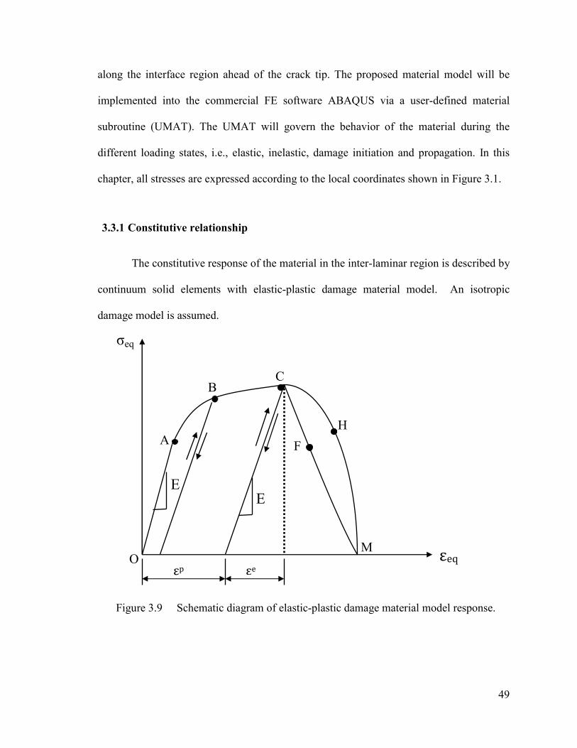
49

along the interface region ahead of the crack tip. The proposed material model will be

implemented into the commercial FE software ABAQUS via a user-defined material

subroutine (UMAT). The UMAT will govern the behavior of the material during the

different loading states, i.e., elastic, inelastic, damage initiation and propagation. In this

chapter, all stresses are expressed according to the local coordinates shown in Figure 3.1.

3.3.1 Constitutive relationship

The constitutive response of the material in the inter-laminar region is described by

continuum solid elements with elastic-plastic damage material model. An isotropic

damage model is assumed.

Figure 3.9 Schematic diagram of elastic-plastic damage material model response.

H

F

B C

εeq

σeq

O

A

εp

εe

E E

M

50

In Figure 3.9, a schematic diagram of elastic-plastic damage material model is

shown. The response of the undamaged material which is shown by the initial part of the

curve (OA) is assumed to be linearly elastic. Point A is a yield point where the onset of

permanent strain is initiated. In multi-axial stress state, this yield point is often denoted a

yield/loading surface. The part of the curve (AC) denotes an elasto-plastic response

which is also said to introduce a “hardening” mechanism, with a damage initiation point

at the maximum equivalent stress, point C. This point is denoted by delamination onset

surface in multi-axial stress state. The plastic stiffness during hardening will be

calculated using the hardening law. The portion of CH or CF reflects a “softening”

mechanism and the stiffness of softening will be determined using the damage evolution

criteria. Unloading is assumed to take place as a purely elastic process with the initial

stiffness. Reloading after unloading gives elastic response up to a new yield point B.

The key factors required to describe the basic principle in the elastic-plastic

damage material model are summarized as follows:

1. A decomposition of total strain into elastic and plastic contributions:

p

ij

e

ijij ddd εεε += (3.2)

where ijdε is increment of total strain, e

ijdε is increment of elastic strain, and p

ijdε

is increment of plastic strain

A governing principle for the elastic contribution:

klijkl

e

ij dEd σε 1−= (3.3)

where Eijkl is the initial elastic stiffness

2. Factors that control plastic deformation are:

(a). Yield criterion

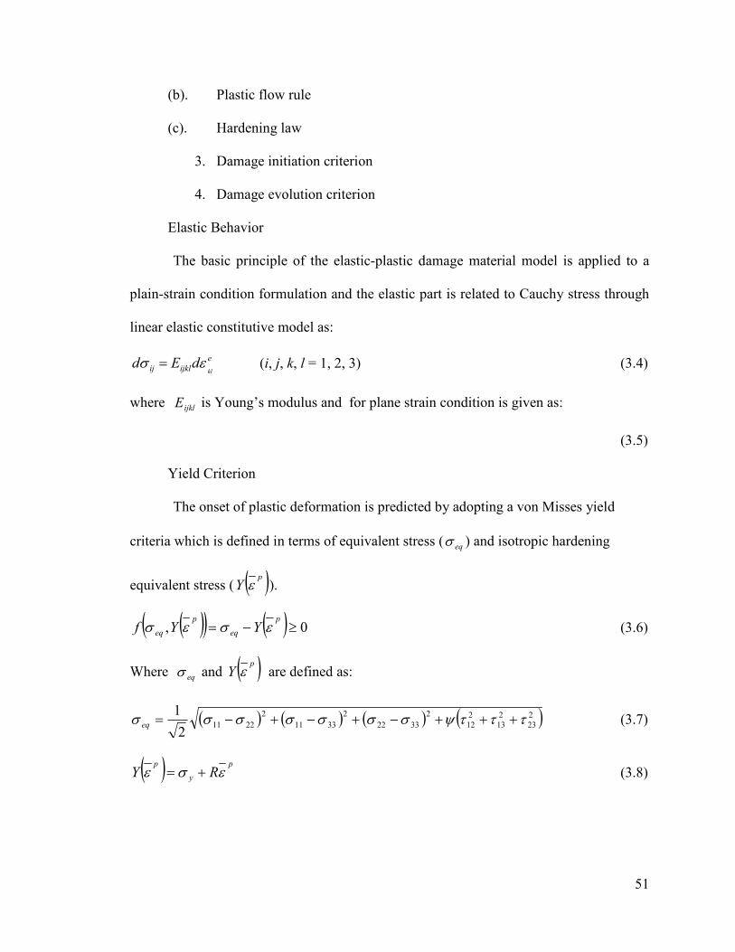
51

(b). Plastic flow rule

(c). Hardening law

3. Damage initiation criterion

4. Damage evolution criterion

Elastic Behavior

The basic principle of the elastic-plastic damage material model is applied to a

plain-strain condition formulation and the elastic part is related to Cauchy stress through

linear elastic constitutive model as:

e

ijklij kldEd εσ = (i, j, k, l = 1, 2, 3) (3.4)

where ijklE is Young’s modulus and for plane strain condition is given as:

(3.5)

Yield Criterion

The onset of plastic deformation is predicted by adopting a von Misses yield

criteria which is defined in terms of equivalent stress ( eqσ ) and isotropic hardening

equivalent stress ( ( )p

Y ε ).

( )( ) ( ) 0, ≥−=p

eq

p

eq YYf εσεσ (3.6)

Where eqσ and ( )p

Y ε are defined as:

( ) ( ) ( ) ( )2

23

2

13

2

12

2

3322

2

3311

2

22112

1τττψσσσσσσσ +++−+−+−=eq (3.7)

( ) p

y

p

RY εσε += (3.8)

52

Where yσ is yield stress, p

ε is an accumulated plastic strain and R represents the slope

of the isotropic strain hardening (see Figure 3.10). The corresponding equivalent total

strain is:

( ) ( ) ( ) ( )2

23

2

13

2

12

2

3322

2

3311

2

22113

2εεεψεεεεεεε +++−+−+−=eq (3.9)

The parameter ψ in Eqns. (3.7) and (3.9) is defined in terms of the tensile (T) and shear

strength (S) of the material in the inter-laminar region. The expression for ψ is derived

based on the assumption that ( )3322 σσ = in Eqn. (3.7) for uniaxial tensile test under ideal

case and making use of the tensile (T) and shear strength (S) of the material as an

allowable stress limit for yielding. For von Mises criterion, 6=ψ .

2

2

=S

Tψ (3.10)

Figure 3.10 Schematic diagram of linear isotropic strain-hardening curve

pε

Y

O

R

yσ

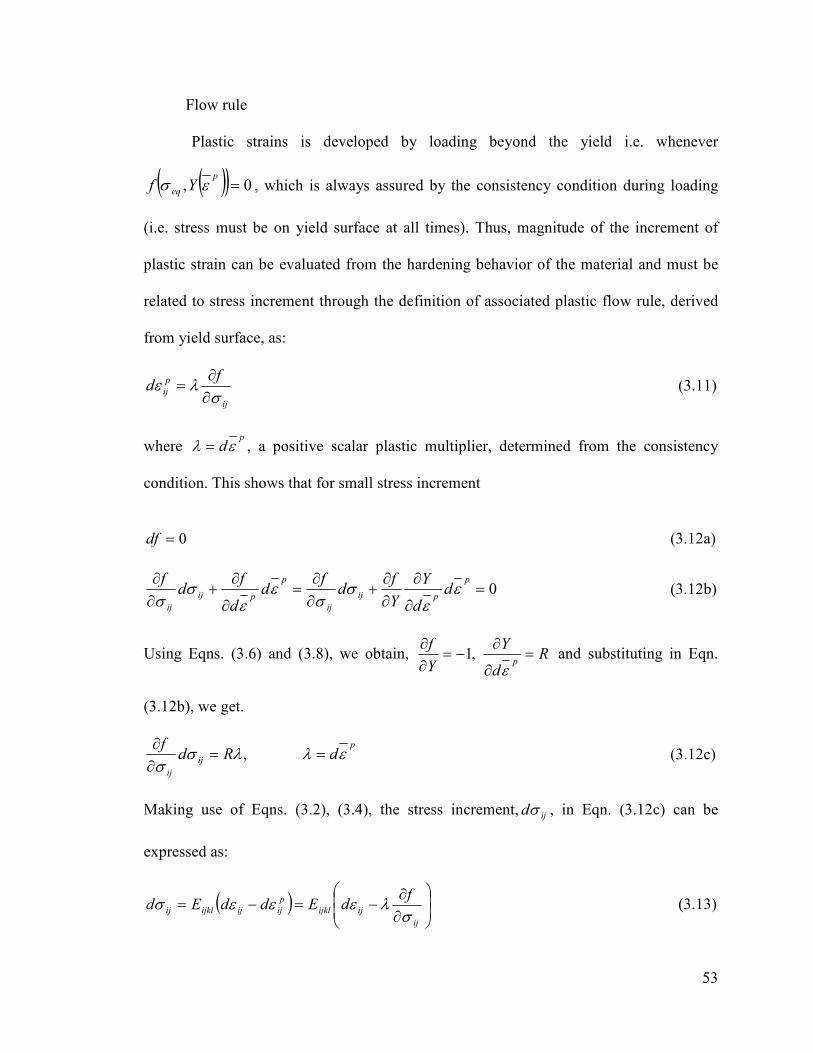
53

Flow rule

Plastic strains is developed by loading beyond the yield i.e. whenever

( )( ) 0, =p

eq Yf εσ , which is always assured by the consistency condition during loading

(i.e. stress must be on yield surface at all times). Thus, magnitude of the increment of

plastic strain can be evaluated from the hardening behavior of the material and must be

related to stress increment through the definition of associated plastic flow rule, derived

from yield surface, as:

ij

p

ij

fd

σλε

∂∂

= (3.11)

where p

dελ = , a positive scalar plastic multiplier, determined from the consistency

condition. This shows that for small stress increment

0=df (3.12a)

0=∂

∂∂∂

+∂∂

=∂

∂+

∂∂ p

pij

ij

p

pij

ij

dd

Y

Y

fd

fd

d

fd

fε

εσ

σε

εσ

σ (3.12b)

Using Eqns. (3.6) and (3.8), we obtain, Rd

Y

Y

fp

=∂

∂−=

∂∂

ε,1 and substituting in Eqn.

(3.12b), we get.

p

ij

ij

dRdf

ελλσσ

==∂∂

, (3.12c)

Making use of Eqns. (3.2), (3.4), the stress increment, ijdσ , in Eqn. (3.12c) can be

expressed as:

( )

∂∂

−=−=ij

ijijkl

p

ijijijklij

fdEddEd

σλεεεσ (3.13)

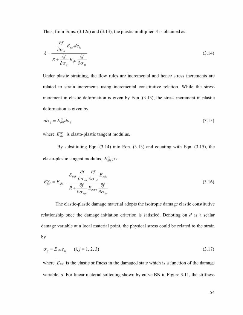
54

Thus, from Eqns. (3.12c) and (3.13), the plastic multiplier λ is obtained as:

kl

ijkl

ij

klijkl

ij

fE

fR

dEf

σσ

εσ

λ

∂∂

∂∂

+

∂∂

= (3.14)

Under plastic straining, the flow rules are incremental and hence stress increments are

related to strain increments using incremental constitutive relation. While the stress

increment in elastic deformation is given by Eqn. (3.13), the stress increment in plastic

deformation is given by

ij

ep

ijklij dEd εσ = (3.15)

where ep

ijklE is elasto-plastic tangent modulus.

By substituting Eqn. (3.14) into Eqn. (3.13) and equating with Eqn. (3.15), the

elasto-plastic tangent modulus, ep

ijklE , is:

rs

mnrs

mn

cdkl

cdab

ijab

ijkl

ep

ijkl fE

fR

Eff

E

EE

σσ

σσ

∂∂

∂∂

+

∂∂

∂∂

−= (3.16)

The elastic-plastic damage material adopts the isotropic damage elastic constitutive

relationship once the damage initiation criterion is satisfied. Denoting on d as a scalar

damage variable at a local material point, the physical stress could be related to the strain

by

klijklij E εσ = (i, j = 1, 2, 3) (3.17)

where ijklE is the elastic stiffness in the damaged state which is a function of the damage

variable, d. For linear material softening shown by curve BN in Figure 3.11, the stiffness

55

in the damaged state can be determined from the geometry of the same figure and is

given by

( )

+−−=

dUdU

dUEE

c

c

ijklijkl

21

21

0

(3.18)

where UC is critical strain energy at a complete failure of the loaded element and is

considered as a material property. U0 is the strain energy when damage initiation occurs

in the material for the first time and can be calculated as:

10 |)( ≥∫= eijij dU εσ (i, j = 1, 2, 3) (3.19)

where e is a non-dimensional parameter that is used to show the condition for damage

initiation in a material. The value ( 1≥e ) indicates a critical condition for damage

initiation is reached and the details will be discussed later in section 3.3.2.

The range of d value is from 0 (without damage) to 1 (completely damaged). When

the damage is fully developed, i.e. d = 1, the stiffness given by Eqn. (3.18) drops to zero

and the material cannot withstand any types of load. Since this result possibly leads to the

penetration between the neighboring substrates in FRP, stiffness degradation in the out-of-

plane direction (2-direction in Figure 3.1) is prohibited when the compressive strain

occurs in that direction.

56

Figure 3.11 Schematic diagram of elastic-plastic damage material model with linear

softening

In Figure 3.11, DU is the energy absorbed by any deformation mode at the current

loading state after delamination is initiated and can be determined by integrating the

energy dissipated in a given fracture mode. For example, for a linear material softening

condition, at the current loading state shown in Figure 3.11, DU is given by the area

(ADBC) as:

)(2

)(

0

0

UU

UU

C

CC

D −

−=

εεσ (3.20)

U0 = ADBF

UD= ADBC

UC =ADBN

E

A

O

C Current state

E

σy

D F L N

σeq Damage initiation B

εeq

σc

E

ε* ε0 ε εf

57

where Cσ and 0ε are the maximum equivalent stress and corresponding equivalent

strain, respectively, when a damage initiation criterion is satisfied at the first time, and ε

is the equivalent strain at the current stress state.

The value range for DU is from 0 (when 0εε = ) to CU , i.e., when the damage is

fully developed (d = 1 at which fεε = ). When d = 1, the dissipated energy reaches its

critical value, CU .

3.3.2 Damage initiation criterion

Depending on the normal stress component ( 22σ ) being positive or negative, the

following damage initiation criterion is proposed.

2 2 22 2 211 22 11 22 11 33 22 33 3312 13 222

2

2 2 22 2 2 2 11 22 11 22 11 33 22 33 3312 13 222

( )( ) ( ) / (for 0)

( )( ) / ( ) (for 0)

ST

e

ST

σ σ σ σ σ σ σ σ στ τ σ

σ σ σ σ σ σ σ σ στ τ α σ

+ − + + ++ + >

= + − + + + + − ≤

(3.21)

where 12τ and 13τ are shear stresses, α a non-dimensional parameter that is used to

quantify the effect of the compressive stress on the suppression of delamination and is

determined using the critical load for damage initiation, T and S are transverse tensile and

shear strength of the material in the interface, respectively. The value of e determines

whether the critical condition for damage initiation is reached. That is, the damage is

initiated when e is equal to or larger than 1.

The damage initiation criterion reflects the phenomenon that compressive stress

may slow down or suppress the damage initiation [29].

58

3.3.3 Damage evolution law

As shown in Eqn. (3.18), the material softening is fully governed by the evolution

of a damage variable d. The damage parameter d can be defined by any monotonically

increasing function, valued from 0 to 1, of any state variables such as stresses, strains or

strain energy. In this study, the evolution of d is expressed in terms of the critical strain

energy ( CU ) and the present state of energy absorbed by the deformation ( DU ).

m

CDC

m

D

UUU

Ud

+−= (3.22a)

where m is a non-dimensional parameter selected to allow change of damage evolution

law. For a linear system, m= 1, the value of d is:

DC

D

UU

Ud

−=

2 (3.22b)

Figure 3.12 Schematic diagram of evolution of damage parameter as a function of

dissipated energy

Ud

d

59

Figure 3.12 shows the evolution of the damage parameters d for different value of

m. The value of d starts from 0, following different paths to 1 for complete damage,

depending on the value of m. In the case of strain increase monotonically, the value of d

also increases monotonically to indicate the damage development. In the case of strain

reverse, d will remain at its historically high value. This is to reflect the fact that damage

is irreversible in the material. It should be noted that with the change of m value, the

expression of d generates different shape of stress-strain curves during the damage

evolvement.

3.4 Application to pre-cracked composites

The elastic-plastic damage material model proposed here was implemented in a

finite element code ABAQUS/Standard using a user subroutine UMAT. The damage

material model is applied to DENT, DCB and INF finite element models under plain strain

condition. The DCB and INF tests cover the scenario for stable delamination under pure

mode I and II loading, respectively. In both tests, the delamination is assumed to grow in

the interlaminar region within the mid-plane. The DENT test is for a model of

homogenous property, covering the loading scenarios for Mode I. The stress-strain

response under different loading conditions will be obtained by applying appropriate loads

and boundary conditions to the FE models. Details of the configurations of these test

specimens are given in the subsequent sections.

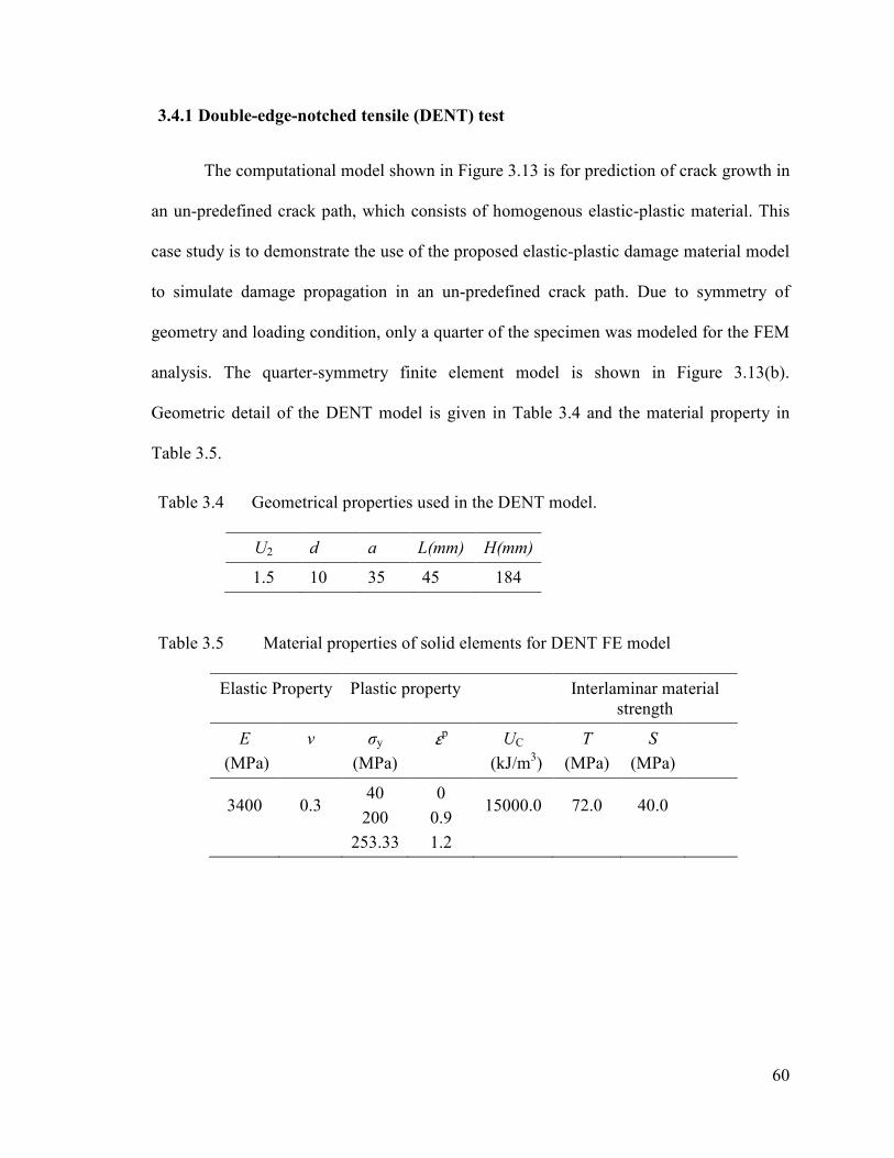
60

3.4.1 Double-edge-notched tensile (DENT) test

The computational model shown in Figure 3.13 is for prediction of crack growth in

an un-predefined crack path, which consists of homogenous elastic-plastic material. This

case study is to demonstrate the use of the proposed elastic-plastic damage material model

to simulate damage propagation in an un-predefined crack path. Due to symmetry of

geometry and loading condition, only a quarter of the specimen was modeled for the FEM

analysis. The quarter-symmetry finite element model is shown in Figure 3.13(b).

Geometric detail of the DENT model is given in Table 3.4 and the material property in

Table 3.5.

Table 3.4 Geometrical properties used in the DENT model.

U2 d a L(mm) H(mm)

1.5

10 35 45 184

Table 3.5 Material properties of solid elements for DENT FE model

Elastic Property Plastic property Interlaminar material

strength

E

(MPa)

v σy

(MPa)

εp

UC

(kJ/m3)

T

(MPa)

S

(MPa)

3400

0.3

40

200

253.33

0

0.9

1.2

15000.0

72.0

40.0

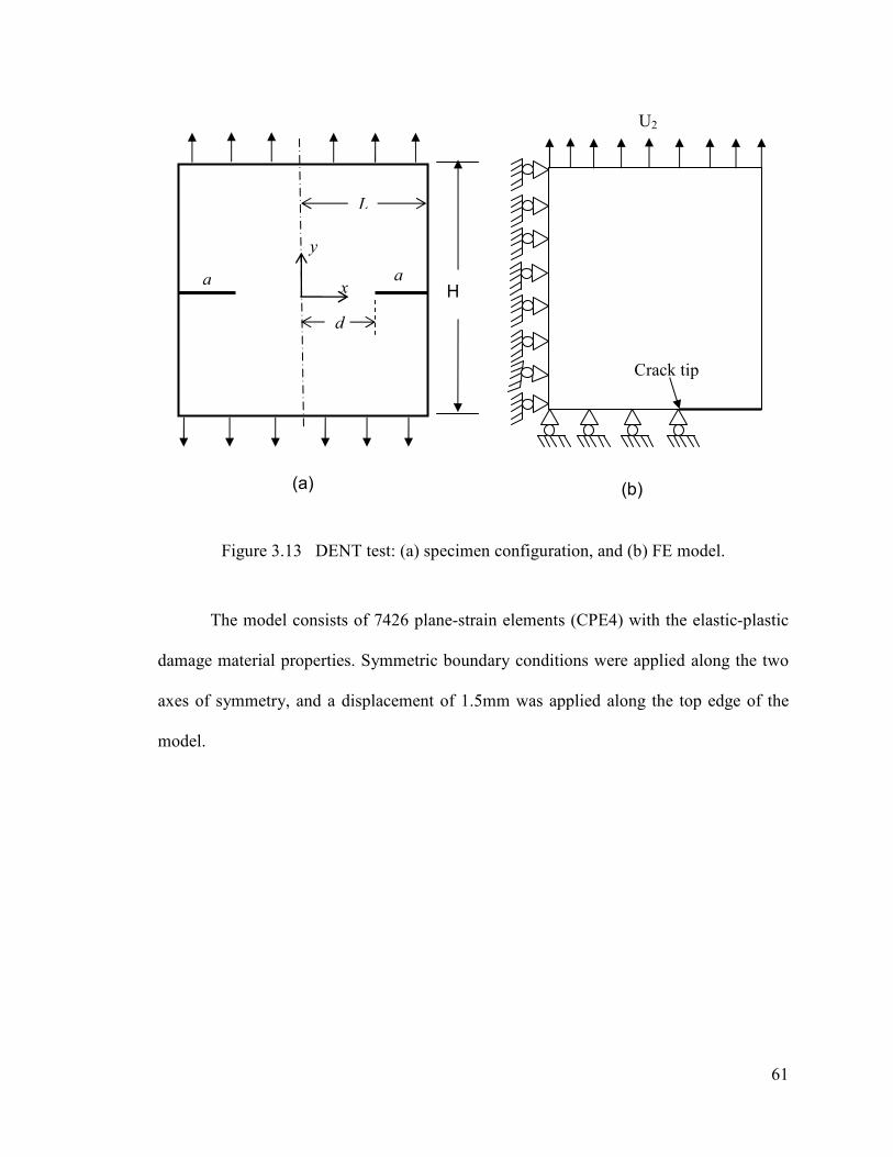
61

Figure 3.13 DENT test: (a) specimen configuration, and (b) FE model.

The model consists of 7426 plane-strain elements (CPE4) with the elastic-plastic

damage material properties. Symmetric boundary conditions were applied along the two

axes of symmetry, and a displacement of 1.5mm was applied along the top edge of the

model.

(a)

Crack tip

U2

(b)

a

L

a

y

x

d

H

62

Figure 3.14 Stress-Strain curve and development of damage process in DENT test

(a)

(c)

(b)

N

A

D

C

B

F L O

(d)

63

Figure 3.14(a) shows the stress-strain relationship of the DENT model subjected

to vertical displacement along the top edge. Vertical and horizontal axes of the curve in

Figure 3.14(a) represent the equivalent stress ( eqσ ) and total strain ( eqε ), respectively.

Point B in Figure 3.14(a) refers to the moment when the damage initiation

criterion is met, i.e. the equivalent stress reaching a critical value of 74MPa and the

corresponding equivalent strain 30%. The area DBF equals the strain energy, U0. Beyond

point B the equivalent stress drops gradually with the increase of the equivalent strain.

At any point during damage evolvement, such as point C in Figure 3.14(a), the

total input of energy density is the area of OABCL, which can be divided into areas

OABD, DBC and DCL, representing the dissipated energy due to plastic deformation, the

unrecoverable energy loss due to material damage (Ud) and the recoverable elastic strain

energy, respectively. If the applied load on the DENT specimen continues to increase from

this point, the load carrying capacity of the element will continue to drop due to decrease

of the equivalent stress following the line segment CN, till point N at which unrecoverable

energy loss, area DBN, equals UC. At this point the equivalent stress is zero. Figure 3.15

displays an equivalent stress contour plot to identify the damaged region with zero

equivalent stress.

If unloading is applied at point C, the equivalent stress will return to zero linearly

following the line segment CD in Figure 3.14(a), at a slope E which is determined by

Eqn. (3.18).

Figures 3.14(b) and 3.14(c) illustrate the evolution of the damage parameters d and

the dissipated energy loss (Ud) during the damage process. Both curves in Figures 3.14(b)

and (c) start at point B and increase monotonically to point N at which a complete damage

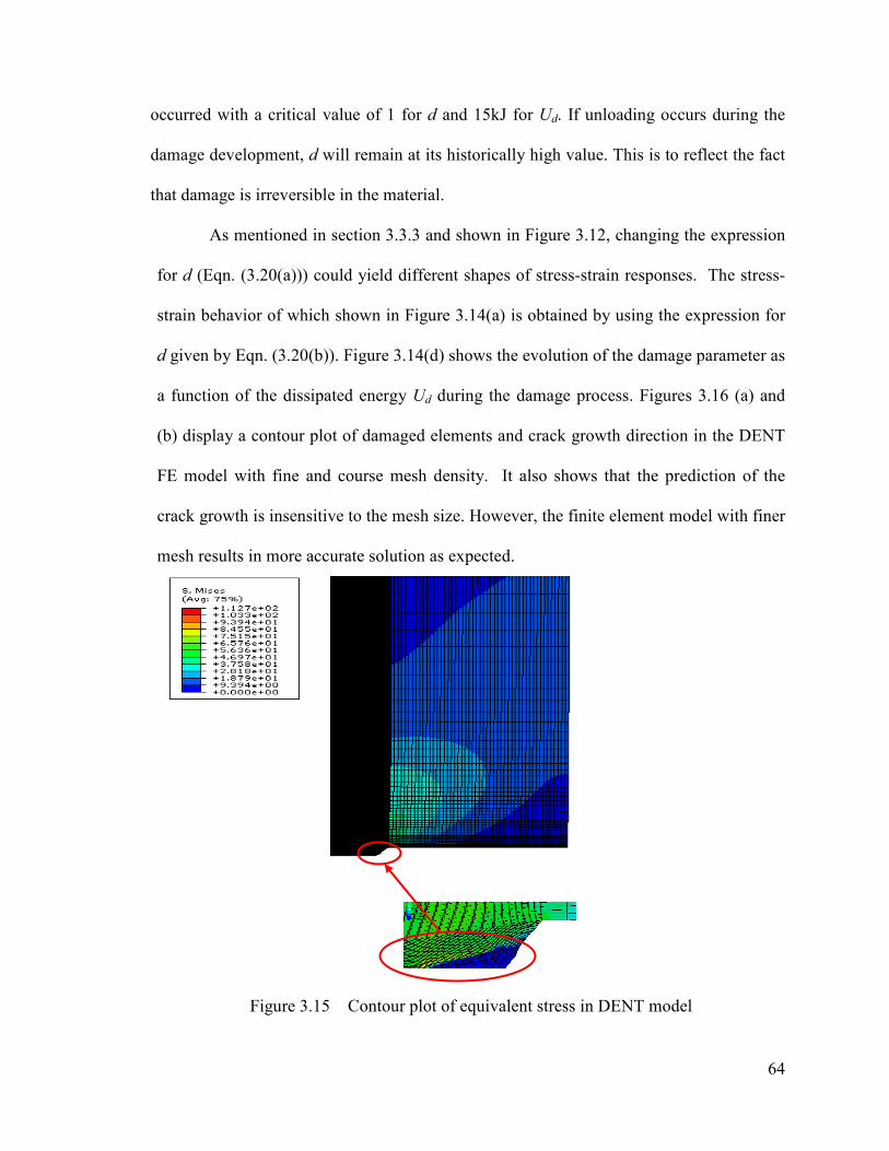
64

occurred with a critical value of 1 for d and 15kJ for Ud. If unloading occurs during the

damage development, d will remain at its historically high value. This is to reflect the fact

that damage is irreversible in the material.

As mentioned in section 3.3.3 and shown in Figure 3.12, changing the expression

for d (Eqn. (3.20(a))) could yield different shapes of stress-strain responses. The stress-

strain behavior of which shown in Figure 3.14(a) is obtained by using the expression for

d given by Eqn. (3.20(b)). Figure 3.14(d) shows the evolution of the damage parameter as

a function of the dissipated energy Ud during the damage process. Figures 3.16 (a) and

(b) display a contour plot of damaged elements and crack growth direction in the DENT

FE model with fine and course mesh density. It also shows that the prediction of the

crack growth is insensitive to the mesh size. However, the finite element model with finer

mesh results in more accurate solution as expected.

Figure 3.15 Contour plot of equivalent stress in DENT model

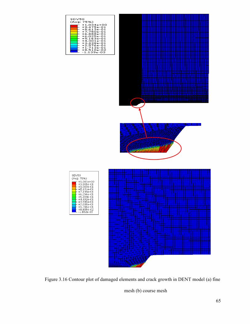
65

Figure 3.16 Contour plot of damaged elements and crack growth in DENT model (a) fine

mesh (b) course mesh

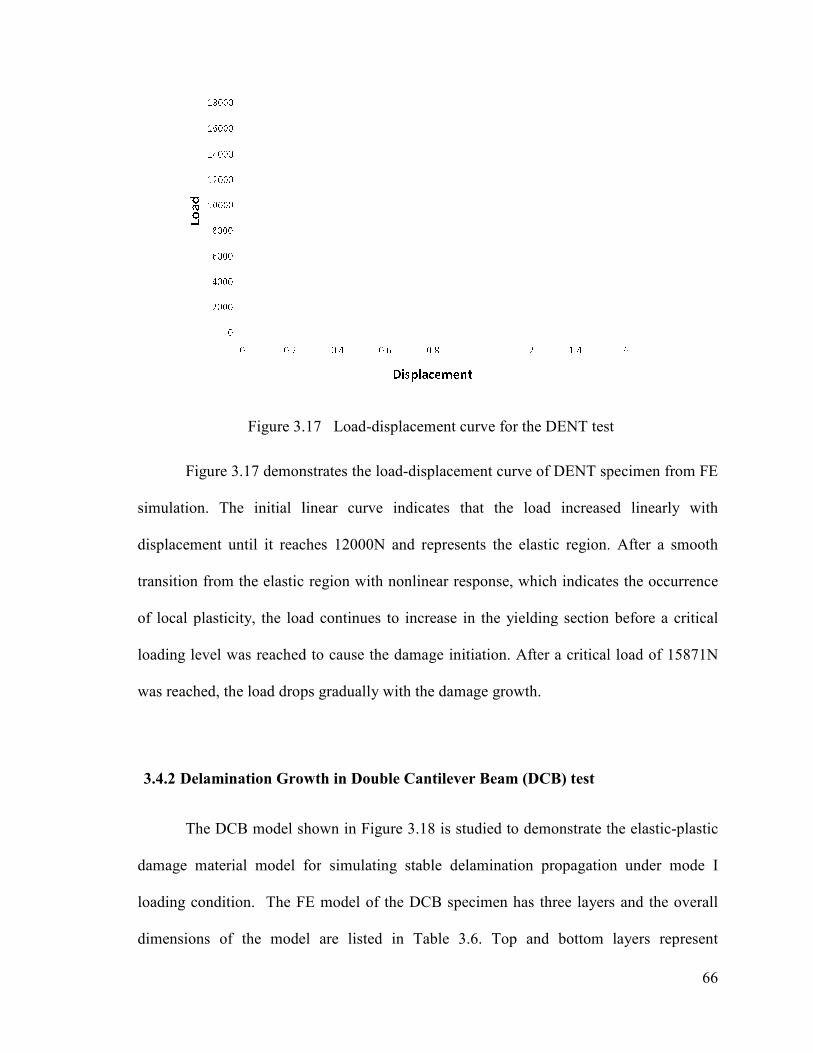
Figure 3.

Figure 3.17 demonstrates the load

simulation. The initial linear curve indicates that the load increased linearly with

displacement until it reaches 12000N and represents the elastic region. Afte

transition from the elastic region with nonlinear response, which indicates the occurrence

of local plasticity, the load continues to increase in the yielding section before

loading level was reached

was reached, the load drops gradually with the damage growth.

3.4.2 Delamination Growth in

The DCB model shown in Figure 3.1

damage material model for

loading condition. The FE model of the DCB

dimensions of the model are listed in Table 3.

.17 Load-displacement curve for the DENT test

Figure 3.17 demonstrates the load-displacement curve of DENT specimen from FE


displacement until it reaches 12000N and represents the elastic region. Afte


of local plasticity, the load continues to increase in the yielding section before

loading level was reached to cause the damage initiation. After a critical load of 15871N

was reached, the load drops gradually with the damage growth.

Delamination Growth in Double Cantilever Beam (DCB) test

The DCB model shown in Figure 3.18 is studied to demonstrate the

for simulating stable delamination propagation under mode I

The FE model of the DCB specimen has three layers and the overall

dimensions of the model are listed in Table 3.6. Top and bottom layers

66

or the DENT test

displacement curve of DENT specimen from FE


displacement until it reaches 12000N and represents the elastic region. After a smooth


of local plasticity, the load continues to increase in the yielding section before a critical

ter a critical load of 15871N

is studied to demonstrate the elastic-plastic

simulating stable delamination propagation under mode I

has three layers and the overall

p and bottom layers represent

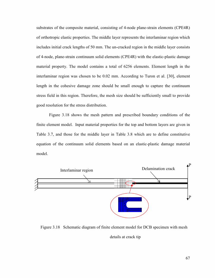
67

substrates of the composite material, consisting of 4-node plane-strain elements (CPE4R)

of orthotropic elastic properties. The middle layer represents the interlaminar region which

includes initial crack lengths of 50 mm. The un-cracked region in the middle layer consists

of 4-node, plane-strain continuum solid elements (CPE4R) with the elastic-plastic damage

material property. The model contains a total of 6256 elements. Element length in the

interlaminar region was chosen to be 0.02 mm. According to Turon et al. [30], element

length in the cohesive damage zone should be small enough to capture the continuum

stress field in this region. Therefore, the mesh size should be sufficiently small to provide

good resolution for the stress distribution.

Figure 3.18 shows the mesh pattern and prescribed boundary conditions of the

finite element model. Input material properties for the top and bottom layers are given in

Table 3.7, and those for the middle layer in Table 3.8 which are to define constitutive

equation of the continuum solid elements based on an elastic-plastic damage material

model.

Figure 3.18 Schematic diagram of finite element model for DCB specimen with mesh

details at crack tip

P

Interlaminar region Delamination crack P

68

Table 3.6. Dimensions of the FE model of DCB specimen

Table 3.7. Mechanical properties for top and bottom layers of the DCB FE model used

in this study

E11

(GPa)

E22 = E33

(GPa)

G12 = G13

(GPa) v23 v12 = v13

150 11.0 6.0 0.3 0.3

Table 3.8 Properties of solid elements in the interlaminar region of the DCB FE

model


strength

E

(MPa)

v σy

(MPa)

εp

UC

(kJ/m3)

T

(MPa)

S

(MPa)

3400

0.3

40

200

253.33

0

0.9

1.2

5000.0

20.0

20.0

Contour plots of equivalent stress and damage level around the crack tip are shown

in Figure 3.19 by applying the elastic-plastic damage material model to the inter-laminar

region. Due to loading symmetry and boundary conditions in the DCB specimen, the

delamination is expected to start from the mid plane, which is indeed indicated by Figure

3.19(b) and 3.19(c). This supports that the proposed damage material model can

accurately predict the delamination growth path in the DCB specimen. Figure 3.20

presents the FE results when the elastic-plastic damage material property in Table 3.8, is

a

(mm)

h

(mm)

L

(mm)

w

(mm)

50 1.5 150 20

69

applied to the entire DCB model. However, because of a sever distortion of the damaged

elements around the crack front, simulation cannot proceed further for the crack growth.

Since there will not be interfacial penetration between the adjacent delaminated surfaces

under mode I loading, those highly distorted damaged elements that do not take any load

(stress) could be deleted from the FE model to advance the simulation. Because of the use

of UMAT subroutine in ABQUS/Standard which doesn’t support element deletion in real

time during the simulation, this problem couldn’t be solved and require further study in

the future.

Figure 3.19 FE result of DCB test with the proposed damage material applied to the

interlaminar region: (a) Contour plot of equivalent stress on FE model (b)

contour plot of damage level around the crack tip in the early stage, (c)

contour plot of the damage level around crack tip during the delamination

growth

(b) (a) (c)

70

Figure 3.20 FE results of DCB specimen with the proposed damage material property

applied to the entire FE model: (a) Contour plot of equivalent stress, (b)

contour plot of damage parameter around crack tip at the early stage, and (c)

contour plot of the damage parameter around the crack tip during the

delamination growth.

3.4.3 Delamination Growth in INF Specimen Under three-point bending

Delamination growth in the INF model, as shown in Figure 3.21, is studied using

continuum solid elements with elastic-plastic damage material property. Similar to the

previous DCB model, the FE model of the INF specimen has three layers and the overall

dimensions of the model are listed in Table 3.1. Top and bottom layers represent

substrates of the composite material, consisting of 4-node plane-strain elements (CPE4I)

with incompatible mode of orthotropic elastic properties. The middle layer represents the

interlaminar region which includes initial crack lengths of 40 mm for a1 and 12 mm for a2.

The un-cracked region in the middle layer consists of 4-node, plane-strain continuum solid

elements (CPE4R) with the elastic-plastic damage material property. Totally, 10421

elements were used for the top and bottom layers, and 6540 elements for the middle layer.

A frictionless, small sliding contact is defined between the crack surfaces to avoid

penetration. The specimen is subjected to a displacement of 4mm at the central loading

pin. A frictionless and small sliding contact condition is defined in the pre-cracked

(a) (b) (c)

71

surfaces. The nodal points at the two supporting pins were restricted from any vertical

motion during the delamination growth. Besides, the nodal point at the left support was

constrained from any horizontal movement to avoid rigid body motion. Input material

properties for the top and bottom layers are given in Table 3.2, and those for the middle

layer in Table 3.9 which are for defining constitutive equation of the continuum solid

elements based on an elastic-plastic damage material model.

Table 3.9 Properties of solid elements at the interlaminar interface of the INF FE

model


strength

E

(MPa)

v σy

(MPa)

εp

UC

(kJ/m3)

T

(MPa)

S

(MPa)

3400

0.3

40

200

253.33

0

0.9

1.2

5000.0

72.0

40.0

Material properties chosen for the interlaminar region, such as tensile (T) and

shear (S) strengths, are based on properties of the resin used in the simulation. The

critical strain energy (UC), yield stresses and equivalent plastic strains are virtual data for

the purpose of testing the proposed damage model.

Figure 3.21 Finite element model of INF test

Interlaminar region Delamination crack

P

72

The results from the 2D model are given in Figures 3.22-3.24. Distribution of the

equivalent stress in Figure 3.22 shows the highest stress concentration at the interface

between the outer substrate and the interlaminar region. Such a stress concentration is

probably caused by the mismatch of material property at the interface and can cause

damage initiation from corners of the crack tip. To minimize such stress concentration

effect, the crack tip is modeled with circular profile within the interlaminar region.

Figures 3.23 demonstrates the deformed shape in front of the crack tip, resulting in

compression on the top half and tension on the bottom half of the interlaminar region.

Figures 3.24 show the location of damage initiation along the contour of the crack tip and

its growth path in the interlamianr region. It is interesting to note that the crack initiation

and its growth path from the crack tip are influenced by the values of the tensile and

shear strengths of the material in the interlaminar region. In figure 3.24(a), the crack

initiation occurs a little below the top corner of the crack tip and subsequently the crack

grows in the interlaminar region. In this case the crack initiation is probably caused by

shear failure of the material, not the tensile failure. When the tensile strength of the

material is lower than its shear strength as shown figure 3.24(b) and 3.24(c), the crack

initiation occurs around the bottom corner of the crack tip. This may be caused by tensile

failure of the material, not the shear failure. Such initiation of local crack due to tensile

failure in a mode II loading test was also reported in ref. [32]. Further study is required

to examine the effect of material tensile and shear strengths on the damage initiation for

delamination. In figure 3.24(c), the crack grows towards the substrate/matrix interface.

Similar to the FE results for the DCB specimen, distortion of damaged elements

due to high plastic strain in the INF specimen model causes instabilities and inhibits

73

further crack growth progress. However, unlike the DCB specimen, care has to be taken

when removing those highly distorted elements from the INF test as this may cause

penetration between adjacent delaminated surfaces. Since the fully damaged elements in

the INF specimen can still take compressive forces to avoid penetration, due to, removing

those elements may increase cause penetration. Another problem from deleting elements

in the INF test is the contact condition. When new fracture surfaces are created after

deleting the elements, the contact algorithm in ABAQUS has to calculate new contact

surfaces, and the associated contact forces, which may cause numerical instabilities. This

suggests that the contact calculation is much easier if elements were not required to be

deleted. All of those problems need further investigation.

Figure 3.22 Contour plot of equivalent stress distribution in INF test

Figure 3.23 Contour plot of equivalent stress around crack tip in the INF test with

T=70MPa and S=40MPa

(a) (b) (c) (d) (e)

Figure 3.24 Contour plot of damage parameter

and S=40MPa (b)

Figure 3.25

Figure 3.25 shows the stress

applying three-point bending

curve profile is similar to the

earlier sections.

(a)

Contour plot of damage parameter in the INF specimen with (a)

=40MPa (b) T=30MPa and S=40MPa (c) T=25MPa and

Stress-strain curve of INF model from FE simulation

shows the stress-strain response of the INF model obtained by

point bending with properties given in Tables (3.1), (3.2

lar to the stress-strain curve of the DENT specimen presented in the

(b)

74

NF specimen with (a) T=70MPa

=25MPa and S=40MPa

simulation

model obtained by

h properties given in Tables (3.1), (3.2) and (3.9). The

the DENT specimen presented in the

(c)

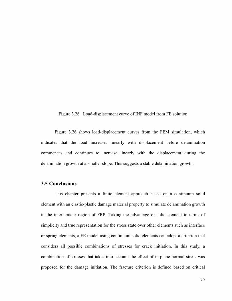
Figure 3.26 Load

Figure 3.26 shows

indicates that the load increases linearly

commences and continues to increase linearly with the displacement during th

delamination growth at a smaller slope. This suggests a stable delamination growth.

3.5 Conclusions

This chapter presents a finite element approach based on a continuum solid

element with an elastic-plastic damage material property

in the interlamianr region of FRP. Taking the advantage of solid element in terms of

simplicity and true representation for the stress state over other elements such as interface

or spring elements, a FE model using continuum solid elements can adopt

considers all possible combinations of stresses for crack initiation. I

combination of stresses that takes into account the effect of in

proposed for the damage initiation. The fracture criterion is

oad-displacement curve of INF model from FE solution

Figure 3.26 shows load-displacement curves from the FEM simulation, which

hat the load increases linearly with displacement before delamination

commences and continues to increase linearly with the displacement during th



plastic damage material property to simulate delamination g



or spring elements, a FE model using continuum solid elements can adopt

considers all possible combinations of stresses for crack initiation. I

that takes into account the effect of in-plane normal stress was

osed for the damage initiation. The fracture criterion is defined based on critical

75

from FE solution

from the FEM simulation, which

before delamination

commences and continues to increase linearly with the displacement during the



simulate delamination growth



or spring elements, a FE model using continuum solid elements can adopt a criterion that

considers all possible combinations of stresses for crack initiation. In this study, a

plane normal stress was

defined based on critical

76

strain energy. The proposed damage material model was implemented in finite element

code ABAQUS and was applied to pre-cracked composites to verify the damage criteria.

It is shown that with a simple linear softening function for the damage evolution, the

proposed damage material model can predict the delamination development in a pure

mode of fracture in fiber composites. The elastic-plastic damage material model was

applied to pre-cracked composite structures such as the DCB, INF and DENT tests.

77

Chapter 4 Conclusions and Future Work

4.1 Summary and Conclusions

Methodologies are discussed for the prediction of stable delamination development

in fiber-reinforced composites in pure mode II fracture using analytical and numerical

methods. Analytical and numerical approaches are described to quantify critical energy

release rate, which is the parameter to measure delamination resistance of the composites.

This thesis presented a revised analytical approach for calculating the compliance

of the INF test by taking into account loads in the overhanging section of the specimen.

The work shows improvement of the revised analytical solution in its accuracy in

predicting the delamination growth, by taking into account the loads in the overhanging

section. Therefore, the work concludes that the overhanging section cannot be ignored.

The revised analytical solution was also used to explore the influence of load in the

overhanging section on prediction of delamination growth rate generated in the INF

specimen. The results suggest that the delamination growth rate in the INF test is

proportional to the loading rate, thus making it possible to investigate the effect of the

crack growth speed on the critical energy release rate.

The finite element model of a virtual INF specimen was used to validate the

revised expressions for compliance and energy release rate through comparison of the

initial specimen stiffness of both solutions. The INF specimen had cohesive elements in

the interlaminar region to simulate the delamination growth, from which extent of damage

78

in front of the crack tip was quantified. Results from FE model suggested that an extensive

damage exists at the crack tip before delamination growth commences. The FE model,

suggests that the damage zone has a length of 8mm which should effectively extend the

initial crack length. Therefore, the use of a physical crack length to calculate the energy

release rate may severely overestimate the interlaminar fracture toughness. Hence, an

effective crack length, which considers the additional crack length due to the presence of a

damage zone at the crack tip, was used to predict the delamination growth. Expression for

the energy release rate based on the effective crack length yields a value that is very close

to the input critical energy release rate (Gc) input into the cohesive elements.

A finite element approach based on a continuum solid element with an elastic-

plastic damage material property was proposed to simulate delamination growth in the

interlamianr region of FRP. Using solid elements, a combination of stresses that takes

into account the effect of in-plane normal stress was used to establish the criterion for

damage initiation. The criterion for delamination propagation is defined based on critical

strain energy. The proposed damage material model was implemented in finite element

code and was applied to pre-cracked composites to illustrate its feasibility to simulate the

crack development.

In general, the work has successfully used analytical and numerical approaches to

simulate delamination growth in FRP under pure mode II loading.

4.2 Future work

79

Verification of the present damage material approach is still in a preliminary stage

and currently, only applied to pre-cracked composite structures. This approach will be

applied to composites with no pre-cracks to further verify its feasibility and the proposed

damage initiation criteria. Parametric studies will also be carried out using appropriate

test methods to investigate the influence of material strengths and other parameters on the

simulation results.

Additionally, mixed-mode delamination is not addressed in this study, which is a

natural next step for the investigation. Besides, a strategy should be devised to measure

delamination resistance experimentally. In the proposed elastic-plastic damage material

model, the damage initiation criteria and the fracture criterion for delamination evolution

are all based on 3D stress and energy state. Thus, this approach could be extended to 3D

simulations, but a strategy is needed to separate the fracture modes involved in the crack

growth.

80

References

1. Anon. Farnborough 2004 - Good prospects for aerospace composites. Reinforced Plast

2004; 48(8): 42-46. D.J. Wilkins, J.R. Eisenmann, R.A. Camin, W.S. Margolis and R.A.

Benson, “Characterizing Delamination Growth in Graphite-Epoxy, Damage in Composite

Materias,” ASTM-STP-775, 1982, 168-183.

2. Camanho, P.P., Mathews, F.L., 1999 “Delamination onset prediction in mechanically

fastened joints in composite laminates” J. Compos. Mater. 33, 906-927

3. Wang Y, Williams JG. Corrections for Mode II fracture toughness specimens of

composites materials. Composites Sci Technol 1992; 43(3): 251-256.

4. Salpekar SA, Raju IS, O'Brien TK. Strain energy release rate analysis of the end-notched

flexure specimen using the finite-element method. J Composites Technol Res 1988;

10(4): 133-9.

5. Xie D, Waas AM, Shahwan KW, Schroeder JA, Boeman RG. Computation of energy

release rates for kinking cracks based on virtual crack closure technique. CMES -

Computer Modeling in Engineering and Sciences 2004; 6(6): 515-524.

6. Shih CF, Needleman A. Fully plastic crack problems. I. Solutions by a penalty method.

Transactions of the ASME Journal of Applied Mechanics 1984; 51(1): 48-56.

7. Shih CF, Needleman A. Fully plastic crack problems. II. Application of consistency

checks. Transactions of the ASME Journal of Applied Mechanics 1984; 51(1): 57-64.

81

8. A. Turon, P.P. Camanho, J. Costa, C.G. Davila. A damage model for the simulation of

delamination in advanced composites under variable-mode loading. Mechanics of

Materials 38(2006), 1072-1089

9. Z. Zou, S.R. Reid, S. Li. A continuum damage model for delamination in laminated

composites. Journal of the Mechanics and Physics of Solids 51(2003) 333-356

10. Alfano G, Crisfield MA. Finite element interface models for the delamination analysis of

laminated composites: Mechanical and computational issues. Int J Numer Methods Eng

2001; 50(7): 1701-1736.

11. ASTM D5528-01, “Standard Test Method for Mode I Interlaminar Fracture Toughness of

Unidirectional Fiber-Reinforced Polymer Matrix Composites,” Annual Book of ASTM

Standards, Vol. 15.03, 2004.

12. O’Brien, T.K., “Interlaminar Fracture Toughness: The long and winding road to

standardization,” Composites Part B: Engineering, Vol.29, No.1, 1998, pp.57-62.

13. B.R.K Blackman, A.J. Brunner, J.G. Williams, “Mode II fracture testing of composites: a

new look at an old problem,” Engineering Fracture Mechanics 73(2006) 2443-2455.

14. C. Fan, P.-Y. B. Jar, J.J. R. Cheng, “Mode II delamination toughness in glass fiber-

reinforced polymers with bridging fibers and stitching threads,” J.Reinforced Plastics and

Composites 28(14),1689-1703(2009).

15. H.Maikuma, J.W. Gillespie, and J.M. Whitney, “Analysis and Experimental

Characterization of the Center Notch Flexural Test Specimen for Mode II Interlaminar

Fracture,”J Composite Mater,23(8): 756-86.

82

16. C. Fan, P.-Y. B. Jar, J.J. R. Cheng, “Energy-based analysis of delamination development

in fiber-reinforced polymers (FRP) under 3-point bending test” Compos.

Sci.Tech.66,2143-2155(2006).

17. E.Reissner, “The Effect of Shear Deformation on the Bending of Elastic Plates,” J. Appl.

Mech. 12(1945) A-69.

18. Anderson TL. Fracture Mechanics of Polymers. 2nd

ed. Florida: CRC Press LLC; 1995

19. Schuecker, C. and Davidson, B.D.(2000). Evaluation of the Accuracy of the Four-point

Bend End-notched Flexure Test for Mode II Delamination Toughness Determination,

Composites Science and Technology, 60: 2137-2146.

20. Alfano G, Crisfield MA. Finite element interface models for the delamination analysis of

laminated composites: Mechanical and computational issues. Int J Numer Methods Eng

2001; 50(7): 1701-1736.

21. Blackman BRK, Hadavinia H, Kinloch AJ, Williams JG. The use of a cohesive zone

model to study the fracture of fibre composites and adhesively-bonded joints. Int J Fract

2003; 119(1): 25-46.

22. Qiu Y, Crisfield MA, Alfano G. An interface element formulation for the simulation of

delamination with buckling. Eng Fract Mech 2001; 68(16): 1755-76.

23. Mi Y, Crisfield MA, Davies GAO, Hellweg H-. Progressive delamination using interface

elements. J Composite Mater 1998; 32(14): 1246-1272.

24. Turon A, Camanho PP, Costa J, Davila CG. (2004). Interface Damage Model for the

Simulation of Delamination Under Variable-Mode Ratio in Composite Materials. Report

No.: NASA/TM-2004-213277. United States: .

83

25. Turon A, Davila CG, Camanho PP, Costa J. (2005). Engineering Solution for Using

Coarse Meshes in the Simulation of Delamination with Cohesive Zone Models. Report

No.: NASA/TM-2005-213547. United States: .

26. Chengye Fan. Characterization and Prediction of Delamination in Fiber-reinforced

Composites. PhD Dissertation, Department of Mechanical Engineering, University of

Alberta 2007.

27. Chengye Fan, P. –Y. Ben Jar, J.J. Roger Cheng. Cohesive zone with continuum damage

properties for simulation of delamination development in fiber composites and failure of

adhesive joints. Engineering Fracture Mechanics 75(2008) 3866-3880.

28. ABAQUS Version 6.9

29. J.P. Hou, N. Petrinic, C. Ruiz, S.R. Hallett. Prediction of impact damage in composite

plates. Composite Science and Technology 60(2000) 273-281.

30. Turon A, Davila CG, Camanho PP, Costa J. (2005). Engineering Solution for Using

Coarse Meshes in the Simulation of Delamination with Cohesive Zone Models. Report

No.: NASA/TM-2005-213547. United States:

31. Benzeggagh, M.L. and M. Kenane. Measurement of Mixed-Mode Delamination Fracture

Toughness of Unidirectional Glass/Epoxy Composites with Mixed-Mode Bending

Apparatus. Composites Science and Technology 56(1996) 439-449.

32. M. Todo, P.-Y.B. Jar, K. Takahashi. Initiation of a mode-II interlaminar crack from an

insert film in the end-notched flexure composite specimen. Composites Science and

Technology 60(2000) 263-272.

33. Qiang Xu, Zixing Lu. An elastic-plastic cohesive zone model for metal-ceramic

interfaces at finite deformations. International Journal of Plasticity 41(2013) 147-164.

84

34. Song Xin, Liu Zheng, Zhang Jiazhen. Simulation study of fracture behavior in a FML

specimen by 3D elastic-plastic finite element model. Polymers and Polymer Composites,

19(2011) 209-212.

university of alberta · characterization of stable delamination growth in fiber-reinforced...

Documents