universal hyperbolic geometry iii: first steps in projective triangle

KoG•15–2011 N. J. Wildberger: Universal Hyperbolic Geometry III: First Steps in Projective Triangle Geometry

Original scientific paperAccepted 19. 12. 2011.

NORMAN JOHN WILDBERGER

Universal Hyperbolic Geometry III:

First Steps in Projective Triangle Geometry

Universal Hyperbolic Geometry III:

First Steps in Projective Triangle Geometry

ABSTRACT

We initiate a triangle geometry in the projective metricalsetting, based on the purely algebraic approach of universalgeometry, and yielding in particular a new form of hyper-bolic triangle geometry. There are three main strands: theOrthocenter, Incenter and Circumcenter hierarchies, withthe last two dual. Formulas using ortholinear coordinatesare a main objective. Prominent are five particular points,the b, z, x, h and s points, all lying on the Orthoaxis A. Arich kaleidoscopic aspect colours the subject.

Key words: universal hyperbolic geometry, triangle geo-metry, projective geometry, bilinear form, ortholinear co-ordinates, incenter, circumcenter, orthoaxis

MSC 2010: 51M10, 14N99, 51E99

Univerzalna hiperbolicka geometrija III:

Prvi koraci u projektivnoj geometriji trokuta

SAZETAK

Na temelju algebarskog pristupa univerzalne geometrije,uvodimo geometriju trokuta u projektivno-metricki okvir.To rezultira jednim novim oblikom hiperbolicke geometrijetrokuta. Tri su glavne okosnice: hijerarhije ortocentara,sredista upisanih i sredista opisanih kruznica, od kojih suposljednje dvije dualne. Primjena ortolinearnih koordinatau formulama ima bitnu ulogu. Istaknuto je pet poseb-nih tocaka (b, z, x, h i s) koje leze na ortogonalnoj osiA. Bogato, kaleidoskopsko glediste karakterizira obraduteme.

Kljucne rijeci: univerzalna hiperbolicka geometrije, geo-metrija trokuta, projektivna geometrija, bilinearna forma,ortolinearne koordinate, srediste upisane kruznice, sredisteopisane kruznice, ortogonalna os

1 Introduction

Recently there has been a revival of interest in classicalgeometry and in particular the study of triangles ([6], [7],[9], [10], [12], [13], [14]). This paper introduces trianglegeometry into the framework of Universal Hyperbolic Ge-ometry (UHG) ([18], [19]) and beyond; in the context ofa general metrical structure on the projective plane. Thebasic measurements of quadrance and spread replace theusual notions of distance and angle, and these depend ona general bilinear form. Hyperbolic geometry provides themotivation and is used for the illustrations. The approachis purely algebraic and works over any field not of char-acteristic two; the reader may easily keep the fundamen-tal example of the rational number field foremost in mind.Ultimately this theory is a natural consequence of RationalTrigonometry ([15], [16], [17]).Triangle geometry in this setting has features that resem-ble and also contrast with classical hyperbolic geometry,studied and described in [1], [2], [3], [4], [5], [11] and[21]. The Orthocenter hierarchy, involving Altitudes, Or-thic triangles, the Orthic axis, the Double triangle, and theOrthoaxis, on which the important s,h,x,b and z points

are to be found, is primary. The Incenter and Circum-center hierarchies are precisely dual, and their existencesdepend on number theoretic conditions, unlike the usualEuclidean situation. The former contains the Incenters, Bi-lines (analogs of vertex or angle bisectors), Bipoints, Apol-lonius points, Centrian lines, Sight lines, Contact points,Gergonne points and Nagel points etc. The latter containsCircumlines, Midpoints, Midlines (analogs of perpendicu-lar bisectors), Medians, Centroids, Sound points, Tangentlines, Jay lines and Wren lines etc. Duality pervades thesubject; interchanging points and lines, sides and vertices,and quadrance and spread.This paper is largely self-contained; we start with a gen-eral introduction to universal metrical projective geome-try. When we study a triangle a1a2a3, it will prove conve-nient to use a linear transformation to change coordinates,so that we may assume that a1 = [1 : 0 : 0] , a2 = [0 : 1 : 0]and a3 = [0 : 0 : 1] , with the orthocenter represented byh = [1 : 1 : 1]. With these ortholinear coordinates the bilin-ear form is given by a pair of inverse symmetric projectivematrices:

B =

a 1 11 b 11 1 c

, A = B−1 =

1−bc c−1 b−1c−1 1−ac a−1b−1 a−1 1−ab

. (1)

25


This shifts projective triangle geometry from the study ofa general triangle under a particular bilinear form to thestudy of a particular triangle under a general bilinearform, giving a simpler and more general theory.Formulas will be our main aims; most of these dependon the three parameters a,b,c occurring in (1), and hope-fully will provide a solid platform for further investiga-tions. They also suggest a possible alternative to trilinearcoordinates in affine/Euclidean triangle geometry. This pa-per introduces a rich theory which has many additional re-lationships and remarkable aspects which will be furtherstudied in the coming years.

1.1 Projective linear algebra and Universal geometry

In this section we introduce the main objects: (projective)points and lines, via projective linear algebra. This is linearalgebra with vectors and matrices defined only up to non-zero scalar multiples. We write the usual vectors and matri-ces with round brackets, while projective vectors and pro-jective matrices, in square brackets, are by definition un-changed if we multiply all coordinates simultaneously bya non-zero number. So while −→v ≡ (3,1,2) ≡

(

3 1 2)

represents a usual row vector (or 1× 3 matrix), the corre-sponding projective row vector is a =

[

3 1 2]

. By def-inition a is also equal to

[

−3 −1 −2]

or to[

6 2 4]

.We will generally use bold labels to represent projectivematrices: while

A =

2 1 40 3 10 0 1

and B =

3 −1 −110 2 −20 0 6

denote ordinary matrices, the corresponding projective ma-trices are

A =

2 1 40 3 10 0 1

=

6 3 120 9 30 0 3

,

B =

3 −1 −110 2 −20 0 6

=16

3 −1 −110 2 −20 0 6

.

Inverses are easier to compute in the projective setting,since determinants in the denominator can be dispensedwith: for example A−1 = B, so that integer arithmetic onlyis required. While in general projective matrices cannot beadded, they can be multiplied!We now introduce additional notation and terminology thatallows us to work consistently with both row and columnvectors horizontally. A non-zero projective row vector awill be written in either of the following forms:

a ≡

[

x y z]

≡ [x : y : z]

and will be called a (projective) point. A non-zero projec-tive column vector L will be written as

L ≡

lmn

≡ 〈l : m : n〉

and will be called a (projective) line. The point a ≡

[x : y : z] and the line L ≡ 〈l : m : n〉 are incident preciselywhen lx+my+nz= 0; equivalently a lies on L, or L passesthrough a. The corresponding matrix equation is

aL ≡

[

x y z]

lmn

= [x : y : z]〈l : m : n〉 = 0. (2)

Three or more points are collinear precisely when they alllie on a line L, and three or more lines are concurrent pre-cisely when they all pass through a point a.

The join a1a2 of distinct points a1 ≡ [x1 : y1 : z1] and a2 ≡

[x2 : y2 : z2] is the line

a1a2 ≡ [x1 : y1 : z1]× [x2 : y2 : z2]

≡ 〈y1z2 − y2z1 : z1x2 − z2x1 : x1y2 − x2y1〉 .

The meet L1L2 of distinct lines L1 ≡ 〈l1 : m1 : n1〉 andL2 ≡ 〈l2 : m2 : n2〉 is the point

L1L2 ≡ 〈l1 : m1 : n1〉× 〈l2 : m2 : n2〉

≡ [m1n2 −m2n1 : n1l2 −n2l1 : l1m2 − l2m1] .

These operations, using the usual Euclidean cross product,are well-defined, and will be used repeatedly in this paper.The symbol × in the linear algebra context avoids confu-sion with matrix multiplication.Then a1a2 is the unique line incident with both a1 and a2,and L1L2 is the unique point incident with both L1 and L2.A complete symmetry or duality between points and linesis a key feature of this subject.We also recall a few more definitions from [18] and [19].A side a1a2 ≡ {a1,a2} is a set of two points. A ver-tex L1L2 ≡ {L1,L2} is a set of two lines. A trianglea1a2a3 ≡ {a1,a2,a3} is a set of three non-collinear points,and a trilateral L1L2L3 ≡{L1,L2,L3} is a set of three non-concurrent lines.

A triangle a1a2a3 determines an associated trilateralL1L2L3, where L1 ≡ a2a3, L2 ≡ a1a3 and L3 ≡ a1a2. Sym-metrically a trilateral L1L2L3 determines an associated tri-angle a1a2a3, where a1 ≡ L2L3, a2 ≡ L1L3 and a3 ≡ L1L2.The triangle a1a2a3 has three sides, namely a1a2, a2a3 anda1a3, as well as three vertices, namely L1L2, L2L3 andL1L3. In this paper we concentrate on triangles.

26


1.2 Projective bilinear forms

We now introduce a metrical structure on our three-dimensional vector space; this will be done via a symmet-ric bilinear form−→v 1 ·

−→v 2 ≡−→v 1A−→v T

2 given by an invertiblesymmetric 3×3 matrix A, where −→v 1 and −→v 2 are ordinaryrow vectors, and T denotes transpose. We wish to trans-fer this bilinear form to projective points and lines: let’sstart with perpendicularity. Recall that vectors −→v 1,

−→v 2 areperpendicular precisely when −→v 1 ·

−→v 2 = 0.

Denote by A and B the projective matrices associated toA and its inverse matrix B respectively. Points a1 and a2are perpendicular precisely when a1AaT

2 = 0, and in thiscase we write a1 ⊥ a2. This is a symmetric relation. Du-ally, lines L1 and L2 are perpendicular precisely whenLT

1 BL2 = 0; we write L1 ⊥ L2. It is useful to restate theserelations by introducing a formal notion of duality: the pro-jective point a and the projective line L are dual preciselywhen

L = a⊥ ≡ AaT or equivalently a = L⊥≡ LT B.

So two points, or two lines, are perpendicular preciselywhen one is incident with the dual of the other. It nowfollows that a1 ⊥ a2 precisely when a⊥1 ⊥ a⊥2 , since thelatter condition is

0 =(

AaT1)T B

(

AaT2)

=(

a1AT )

B(

AaT2)

= a1 (AB)(

AaT2)

= a1AaT2 . (3)

A point a is null precisely when it is perpendicular to itself,that is, when aAaT = 0. Dually a line L is null preciselywhen it is perpendicular to itself, that is, when LT BL = 0.

Our main interests are hyperbolic and elliptic geometries,which arise respectively from the special cases

A = J ≡

1 0 00 1 00 0 −1

= B, A = I≡

1 0 00 1 00 0 1

= B.

(4)

But other possibilities are also of interest, and for trianglegeometry also important, as we shall soon see.

1.3 Visualization

The Figures in this paper all come from hyperbolic geome-try: we represent the point a ≡ [x : y : z] by the affine point[X ,Y ] ≡ [x/z,y/z] , and the line L ≡ 〈l : m : n〉 by the linearequation lX + mY + n = 0, which would be the hyperbolicline (l : m : −n) in [18]. Null points are those a for whichx2 + y2

− z2 = 0; the corresponding affine points lie on thenull circle X2 + Y 2 = 1, always in blue. Null lines are

tangent to this null circle. The duality becomes exactlythe projective polarity between points and lines associatedwith the null circle.

a

l

a

l

a

l

1

1

2

2

3

3

22

3

1

LAL

L

2

1

3

A

A

A

Figure 1: A Triangle a1a2a3 and its Dual triangle l1l2l3We will adopt the general convention that triangle geome-try constructs associated to a particular triangle are Cap-italized (a familiar idea for German readers). So Fig-ure 1 shows a Triangle a1a2a3, in yellow, with the nota-tion we will consistently use: the Points of the triangle area1,a2,a3, the Lines are L1 ≡ a2a3, L2 ≡ a1a3,L3 ≡ a1a2,the Dual points are l1 ≡ L⊥

1 , l2 ≡ L⊥

2 , l3 ≡ L⊥

3 , the Duallines are A1 ≡ a⊥1 , A2 ≡ a⊥2 ,A3 ≡ a⊥3 , and the Dual trian-gle is l1l2l3, in light blue. Points and their dual lines aregenerally pictured with the same colour.

1.4 Quadrance and spread

An inverse pair of symmetric projective matrices A andB give us more than perpendicularity: they allow the in-troduction of metrical quantities into algebraic geometry.This has been a blind spot in the history of the subject!The quadrance q(a1,a2) between points a1 and a2, andthe spread S (L1,L2) between lines L1 and L2, are the re-spective numbers

q(a1,a2) ≡ 1−(

a1AaT2)2

(

a1AaT1)(

a2AaT2) and

S (L1,L2) ≡ 1−(

LT1 BL2

)2

(

LT1 BL1

)(

LT2 BL2

) . (5)

While the numerators and denominators of these expres-sions depend on choices of representative vectors and ma-trices for a1,a2,A,L1,L2 and B, the quotients are indepen-dent of scaling, so the overall expressions are indeed well-defined projectively.Clearly q(a,a) = 0 and S (L,L) = 0, while q(a1,a2) = 1precisely when a1 ⊥ a2, and dually S (L1,L2) = 1 preciselywhen L1 ⊥ L2. An argument similar to (3) shows that forpoints a1 and a2,

S(

a⊥1 ,a⊥2)

= q(a1,a2) . (6)

27


Quadrance and spread are undefined if one or both of thepoints or lines involved is null. We will adopt the zerodenominator convention: statements involving a fractionwith zero in the denominator are empty, and a variant:statements involving a proportion with all entries zero areempty.

Example 1 In the hyperbolic case, the quadrance betweena1 ≡ [x1 : y1 : z1] and a2 ≡ [x2 : y2 : z2] is

q(a1,a2) ≡ 1−(x1x2 + y1y2 − z1z2)

2(

x21 + y2

1 − z21)(

x22 + y2

2 − z22)

= −

(y1z2 − y2z1)2 +(z1x2 − z2x1)

2− (x1y2 − y1x2)

2(

x21 + y2

1 − z21)(

x22 + y2

2 − z22) (7)

and the spread between L1 ≡ 〈l1 : m1 : n1〉 and L2 ≡

〈l2 : m2 : n2〉 is

S (L1,L2) ≡ 1−(l1l2 + m1m2 −n1n2)

2(

l21 + m2

1 −n21)(

l22 + m2

2 −n22)

= −

(m1n2 −m2n1)2 +(n1l2 −n2l1)2

− (l1m2 − l2m1)2

(

l21 + m2

1 −n21)(

l22 + m2

2 −n22) .

(8)

Example 2 In the elliptic case, the quadrance betweena1 ≡ [x1 : y1 : z1] and a2 ≡ [x2 : y2 : z2] is

q(a1,a2) ≡ 1−(x1x2 + y1y2 + z1z2)

2(

x21 + y2

1 + z21)(

x22 + y2

2 + z22)

=(y1z2 − y2z1)

2 +(z1x2 − z2x1)2 +(x1y2 − y1x2)

2(

x21 + y2

1 + z21)(

x22 + y2

2 + z22) (9)

and the spread between L1 ≡ 〈l1 : m1 : n1〉 and L2 ≡

〈l2 : m2 : n2〉 is

S (L1,L2) ≡ 1−(l1l2 + m1m2 + n1n2)

2(

l21 + m2

1 + n21)(

l22 + m2

2 + n22)

=(m1n2 −m2n1)

2 +(n1l2 −n2l1)2 +(l1m2 − l2m1)2

(

l21 + m2

1 + n21)(

l22 + m2

2 + n22) .

(10)

Theorem 1 (Null quadrance/spread) If a1 and a2 aredistinct points, then q(a1,a2) = 0 precisely when a1a2 is anull line. If L1 and L2 are distinct lines, then S (L1,L2) = 0precisely when L1L2 is a null point.

Proof. We prove the first statement, the second followsby duality. Suppose that A is a 3× 3 invertible symmetricmatrix with B the adjugate matrix (the inverse of A up to ascalar), so we may write

A≡

a b cb d fc f g

, B≡

dg− f 2 c f −bg b f − cdc f −bg ag− c2 bc−a fb f − cd bc−a f ad−b2

.

Since L ≡ a1a2 is a null line precisely when LT BL = 0,the theorem is a consequence of the following remarkableidentity in the various variables, involving only vectors andthe usual linear algebra:(

(x1,y1,z1)A(x1,y1,z1)T)(

(x2,y2,z2)A(x2,y2,z2)T)

−

−

(

(x1,y1,z1)A(x2,y2,z2)T)2

= (y1z2 − y2z1,z1x2 − z2x1,x1y2 − x2y1) ·B·

· (y1z2 − y2z1,z1x2 − z2x1,x1y2 − x2y1)T . �

In the paper [17] we show that this general projective met-rical geometry obeys exactly the same main trigonometriclaws as those of Universal Hyperbolic Geometry as set outin the paper [18], independent of the quadratic form. Inparticular the laws of trigonometry for hyperbolic and el-liptic geometries, which are both projective theories, areexactly identical. This is indeed Universal Geometry.

1.5 Linear transformations and the Fundamental the-orem of projective geometry

A bilinear form −→v 1 ·−→v 2 = −→v 1A−→v T

2 is transformed whenwe change coordinates. Suppose we have an invert-ible linear transformation T (−→v ) ≡ −→v M = −→w on three-dimensional space, acting on row vectors via right mul-tiplication by an invertible 3× 3 matrix M, with inversematrix N, so that −→w N = −→v . Define a new bilinear form�

by

−→w 1 �−→w 2 ≡ (−→w 1N) · (−→w 2N) = (−→w 1N)A(−→w 2N)

T

= −→w 1(

NANT )

−→w T2 .

So the matrix A for the original bilinear form · becomes thematrix NANT for the new bilinear form �.

The linear transformation T acting on row vectors inducesa projective transformation T on one-dimensional sub-spaces, which are essentially (projective) points, as well astwo-dimensional subspaces, which are essentially (projec-tive) lines. Let M and N be the projective matrices associ-ated to M and N. On points, we define T(a) = aM. To seehow T acts on lines, we use duality; the point a is incidentwith the line L precisely when aL = 0, which is preciselywhen (aM)(NL) = 0, so we require that T(L) ≡ NL. Inthis way incidence is preserved when we apply a lineartransformation to both points and lines.

The notion of perpendicularity is also modified: the pointsa1 and a2 are �-perpendicular precisely when a1N anda2N are perpendicular, in other words precisely when

28


a1(

NANT )

aT2 = 0, while the lines L1 and L2 are �-per-

pendicular precisely when LT1(

MT BM)

L2 = 0. The in-verse pair of symmetric projective matrices

Ã = NANT and ˜B = MT BM

determine new notions of duality: a⊥ = ÃaT andL⊥ = LT

˜B as well as new quadrances and spreads:

q(a1,a2) ≡ 1−

(

a1ÃaT2

)2

(

a1ÃaT1

)(

a2 ÃaT2

) and

˜S(L1,L2) ≡ 1−

(

LT1˜BL2

)2

(

LT1˜BL1

)(

LT2˜BL2

) . (11)

Recall that the Fundamental theorem of projective ge-ometry in this setting is really basic linear algebra: ageneral linear transformation of three-dimensional spacemaps any three linearly independent vectors −→v 1,

−→v 2,−→v 3

to any other three vectors. If in addition we are givena fourth vector −→v 4 = λ1

−→v 1 + λ2−→v 2 + λ3

−→v 3 with noneof λ1,λ2,λ3 zero, then we can send −→v 1,

−→v 2,−→v 3 respec-

tively to (1/λ1,0,0), (0,1/λ2,0), (0,0,1/λ3) , so that −→v 4is sent to (1,1,1) . When we view this projectively, wehave essentially a proof of the Fundamental theorem: wecan construct a projective linear transformation that sendsfour generic projective points a1,a2,a3 and a4 (no threecollinear) respectively to [1 : 0 : 0], [0 : 1 : 0], [0 : 0 : 1] and[1 : 1 : 1].

1.6 An example with the basic Triangle

We illustrate these abstractions in a concrete example. Ourbasic Triangle shown in Figure 2 comes from the hyper-bolic plane where the points originally have the approxi-mate values:

a1≈[−0.4 : 0.4 : 1],a2≈[−0.7 : −0.4 : 1],a3≈[0.1 : 0.1 : 1]

corresponding to the affine points A1 ≈ [−0.4,0.4], A2 ≈

[−0.7,−0.4], A3 ≈ [0.1,0.1]. The following calculationsare subject to round-off and approximation.The Orthocenter, using formulas for hyperbolic geometryaltitudes, is h ≈ [−0.286886 : 0.217349 : 1]. Now

(x,y,z)

−0.4 0.4 1−0.7 −0.4 10.1 0.1 1

= (−0.2869,0.2173,1)

has the solution (x,y,z)≈ (0.586371,0.117125,0.296503).We conclude that the transformation T (v) = vN where

N ≡

0.586371 0 00 0.117125 00 0 0.296503

−0.4 0.4 1−0.7 −0.4 10.1 0.1 1

=

−0.2345484 0.2345484 0.586371−0.0819875 −0.04685 0.1171250.0296503 0.0296503 0.296503

sends (1,0,0), (0,1,0) , (0,0,1) to multiples of(−0.4,0.4,1), (−0.7,−0.4,1), (0.1,0.1,1) respectively,and also (1,1,1) to (−0.2869,0.2173,1).

a

a

a

A

s

h1

10

1

-1

-1

2

3

Figure 2: Basic triangle a1a2a3 with Orthocenter hOrthostar s, and Orthoaxis A

The inverse projective matrix N−1 = M projectively sendsthe points a1,a2,a3 to [1 : 0 : 0] , [0 : 1 : 0] , [0 : 0 : 1] and hto [1 : 1 : 1]. Recalling the definition of J in (4), the bi-linear form in the new standard coordinates is given (ap-proximately) by the pair of projective inverse matricesA = NJNT and B = MT JM, which are

A ≈

−0.2338 −0.0604 −0.1739−0.0604 −0.00480 −0.0385−0.1739 −0.0385 −0.0862

and

B ≈

−0.7173 1 11 −6.745 11 1 −1.692

so that

a ≈−0.7173, b ≈−6.745, c ≈−1.692.

As an application, let’s look at an important point asso-ciated to the Triangle a1a2a3 called the Orthostar s =[a + 2 : b + 2 : c + 2]. In our example this would be thepoint [1.2827 : −4.745 : 0.308] , and to convert that backinto the original projective or hyperbolic coordinates, wewould multiply by N to get

[1.2827 : −4.745 : 0.308]N≈ [0.0973 : 0.5322 : 0.2877]≈

≈ [0.34 : 1.85 : 1]

which agrees approximately with the affine value for s of[0.34,1.85] in Figure 2. In the same spirit, the OrthoaxisA ≡ hs would have standard coordinates

29


[1 : 1 : 1]× [a + 2 : b + 2 : c + 2] = 〈c−b : a− c : b−a〉 ≈≈ 〈5.053 : 0.9747 : −6.0277〉.

Since this is a line, to convert back to the original coordi-nates we would multiply by M on the left:

M

5.0530.9747−6.0277

≈

−47.0818.02−17.42

≈

2.702−1.03

1.0

giving the line 2.702X − 1.03Y + 1 = 0 with projectivecoordinates 〈2.702 : −1.03 : 1〉 or hyperbolic coordinates(−2.702 : 1.03 : 1). The Orthoaxis A appears in Figure 2as the orange line.

1.7 Midpoints, midlines, bilines and bipoints

There are four more important metrical concepts that playa big role in projective triangle geometry. A side ab has amidpoint m precisely when m is a point lying on ab whichsatisfies q(a,m) = q(m,b), and it has a midline M pre-cisely when M is a line passing through a midpoint, per-pendicular to the corresponding line ab of the side. Mid-lines are called perpendicular bisectors in Euclidean ge-ometry; we prefer the more compact terminology, whichemphasizes the duality between midpoints and midlines.Figure 3 shows our standard Triangle a1a2a3 that we willbe using throughout this paper, together with its six Mid-points m and six Midlines M.

a

a

a

m

m

m

m

m

m

1

2

3s

M

M

M

M

M

M

Figure 3: Midpoints m and Midlines M of the Trianglea1a2a3

Dually a vertex KL has a biline B precisely when B is aline passing through KL which satisfies S (K,B) = S (B,L),and it has a bipoint b precisely when b is a point lying on

a biline, perpendicular to the corresponding point KL ofthe vertex. Bilines are called angle or vertex bisectors inEuclidean geometry. Bipoints have no Euclidean analogs.Figure 4 shows the six Bilines B and four of the six Bi-points b of our standard Triangle. Both Figures 3 and4 have interesting collinearities and concurrences that thereader might like to observe; we will explore these later.

a

a

a

b B

BB

B

B

B

b

b b

1

2

3

Figure 4: Bilines B and Bipoints b

We will see that the existence of midpoints and bilines de-pends on certain quadratic equations having solutions, withthe consequence that sides and vertices generally have zeroor two midpoints, or bilines. In a general triangle thereare then several possibilities about which sides and ver-tices have midpoints or bilines. In future work we will ex-plore interesting variants to these concepts which partiallyreplace them when they do not exist.

2 Ortholinear coordinates

2.1 The Orthocenter theorem

Here is a main theorem which will be pivotal in our ap-proach to triangle geometry in this general projective set-ting. There has recently been renewed interest in the Or-thocenter in hyperbolic geometry ([8]); deservedly so.

Theorem 2 (Orthocenter theorem) Suppose that a1a2a3is a triangle which is not a right triangle, so that no twoof the three lines L1 ≡ a2a3, L2 ≡ a1a3 and L3 ≡ a1a2 areperpendicular. Then the altitude lines (or just altitudes)N1 ≡ a1L⊥

1 , N2 ≡ a2L⊥

2 and N3 ≡ a3L⊥

3 are defined andconcurrent. Their common meet, the Orthocenter h, doesnot lie on L1,L2 or L3.

Proof. If a1a2a3 is not a right triangle, then none of thepoints a1,a2,a3 are dual to the opposite lines L1,L2,L3, sothe three altitudes N1 ≡ a1L⊥

1 , N2 ≡ a2L⊥

2 and N3 ≡ a3L⊥

3are well-defined. Set h ≡ N1N2, with the idea of proving

30


that N3 is also incident with h. Now h does not lie on anyof the lines L1,L2 or L3, since otherwise a1a2a3 would bea right triangle, contrary to our assumption. From the Fun-damental theorem of projective geometry, we can apply alinear transformation to change coordinates so that

a1 = [1 : 0 : 0] ,a2 = [0 : 1 : 0] ,a3 = [0 : 0 : 1] ,h = [1 : 1 : 1] .

It follows that

L1 = a2a3 = [0 : 1 : 0]× [0 : 0 : 1] = 〈1 : 0 : 0〉 ,L2 = a1a3 = [1 : 0 : 0]× [0 : 0 : 1] = 〈0 : 1 : 0〉 ,L3 = a1a2 = [1 : 0 : 0]× [0 : 1 : 0] = 〈0 : 0 : 1〉 , (12)

and

N1 = a1h = [1 : 0 : 0]× [1 : 1 : 1] = 〈0 : 1 : −1〉 ,N2 = a2h = [0 : 1 : 0]× [1 : 1 : 1] = 〈1 : 0 : −1〉 .

Suppose that the inverse projective matrix B for thequadratic form in these new coordinates is

B ≡

a d ed b fe f c

.

Then since L1 ⊥ N1

〈1 : 0 : 0〉T B〈0 : 1 : −1〉= [d − e] = 0

and since L2 ⊥ N2

〈0 : 1 : 0〉T B〈1 : 0 : −1〉= [d − f ] = 0.

From these two equations we deduce that e = f , so thatalso

〈0 : 0 : 1〉T B〈1 : −1 : 0〉 = [e− f ] = 0,

which implies that a3h = 〈1 : −1 : 0〉 is indeed perpendic-ular to L3. So N3 = a3L⊥

3 = a3h passes through h, whichdoes not lie on L1,L2 or L3. �

Theorem 3 (Ortholinear forms) If a1 = [1 : 0 : 0], a2 =[0 : 1 : 0], a3 = [0 : 0 : 1] and h = [1 : 1 : 1] is the orthocen-ter of a1a2a3, then either

B =

a 1 11 b 11 1 c

or B =

a 0 00 b 00 0 c

.

The second possibility occurs precisely when a1a2a3 is afully right triangle: any two of its lines are perpendicular.

Proof. This follows from the proof of the previous theo-rem: the orthocenter being h implies that d = e = f . So upto a re-scaling, the possibilities are either d = e = f = 1 ord = e = f = 0.

Let us now consider the second alternative: where

B =

a 0 00 b 00 0 c

and each of a,b,c is non-zero by assumption. This thenyields the dual points of the triangle to be 〈1 : 0 : 0〉T B =[1 : 0 : 0], and also [0 : 1 : 0] and [0 : 0 : 1]. The dual pointsare then exactly the same as the original points, so this is afully right triangle: all three points and lines are mutuallyperpendicular. �

To summarize, we state the following result.

Theorem 4 (Ortholinear coordinates) If the trianglea1a2a3 is not a right triangle, then we may change co-ordinates so that the bilinear form is given by the pair ofprojective matrices

B =

a 1 11 b 11 1 c

, A = B−1 =

1−bc c−1 b−1c−1 1−ac a−1b−1 a−1 1−ab

(13)

which depend only on the three numbers a,b,c, and so thata1,a2,a3 and the orthocenter h have the forms

a1 ≡ [1 : 0 : 0] , a2 ≡ [0 : 1 : 0] , a3 ≡ [0 : 0 : 1] ,h≡ [1 : 1 : 1] .

We say refer to this as the standard bilinear form, andthat a1a2a3 is the standard triangle, or just the Trian-gle. The coordinates of this framework are called ortho-linear coordinates. We will henceforth assume that wehave made this choice of coordinates.The duals of the Altitudes N1 = 〈0 : 1 : −1〉, N2 =〈1 : 0 : −1〉, N3 = 〈1 : −1 : 0〉 are the Altitude points

n1 = NT1 B = [0 : b−1 : 1− c],

n2 = NT2 B = [a−1 : 0 : 1− c],

n3 = NT3 B = [a−1 : 1−b : 0] . (14)

The dual of the Orthocenter h = [1 : 1 : 1] is the Ortholine

H=A [1 : 1 : 1]T =〈b+c−bc−1 : a+c−ac−1 : a+b−ab−1〉.

Theorem 5 (Null points/lines) The point p ≡ [x : y : z] inOrtholinear coordinates is a null point precisely when

(1−bc)x2 +(1−ac)y2 +(1−ab)z2+

+ 2(c−1)xy + 2(b−1)xz+ 2(a−1)yz = 0.

The line L ≡ 〈l : m : n〉 is a null line precisely when

al2 + bm2 + cn2 + 2lm+ 2ln + 2mn = 0.

31


Proof. These follow by using (13) to expand the respectiveconditions

[x : y : z]A [x : y : z]T = 0 and

〈l : m : n〉T B〈l : m : n〉 = 0. �

Corollary 1 Using ortholinear coordinates, the Pointsa1 ≡ [1 : 0 : 0], a2 ≡ [0 : 1 : 0] and a3 ≡ [0 : 0 : 1] are nullpoints precisely when bc = 1,ac = 1 and ab = 1 respec-tively, and the Lines L1 ≡ 〈1 : 0 : 0〉, L2 ≡ 〈0 : 1 : 0〉 andL3 ≡ 〈0 : 0 : 1〉 are null lines precisely when a = 0,b = 0and c = 0 respectively.

Define

D ≡ abc−a−b− c+2. (15)

Then it is straightforward to check that

detB = det

a 1 11 b 11 1 c

= D and

detA = det

1−bc c−1 b−1c−1 1−ac a−1b−1 a−1 1−ab

= −D2.

Theorem 6 (Triangle quadrances and spreads) UsingOrtholinear coordinates, the quadrances q1 ≡ q(a2,a3) ,q2 ≡ q(a1,a3) , q3 ≡ q(a1,a2) and spreads S1 ≡ S (L2,L3) ,S2 ≡ S (L1,L3) , S3 ≡ S (L1,L2) of the standard Trianglea1a2a3 are

q1 =−Da

(ab−1)(ac−1), q2 =

−Db(ab−1)(bc−1)

,

q3 =−Dc

(ac−1)(bc−1)

and

S1 =bc−1

bc, S2 =

ac−1ac

, S3 =ab−1

ab.

These numbers also satisfy

1−q1 =(a−1)2

(ab−1)(ac−1),

1−q2 =(b−1)2

(ab−1)(bc−1),

1−q3 =(c−1)2

(ac−1)(bc−1)(16)

and

1−S1 =1bc

, 1−S2 =1ac

, 1−S3 =1

ab. (17)

Proof. These are straightforward computations. �

Although it will play only a small role in this paper, wealso introduce the most important number associated to theTriangle, and a formula for it in terms of a,b,c.

Theorem 7 (Triangle quadrea) The quadrea A of the tri-angle a1a2a3 is

A ≡ q2q3S1 = q1q3S2 = q1q2S3 =D2

(ab−1)(ac−1)(bc−1).

Proof. This follows directly from the formulas of the pre-vious theorem. �

We cannot help but point out an important trigonometricformula that follows from this: the Extended Spread lawasserts thatS1q1

=S2q2

=S3q3

=A

q1q2q3.

2.2 Cevians, traces, Desargues theorem and Canoni-cal lines

Consider a variable point p ≡ [x : y : z] distinct fromthe Points a1,a2,a3 of the Triangle a1a2a3. The linesa1 p,a2 p,a3 p are the Cevian lines, or just Cevians, of p.These are

a1 p = [x : y : z]× [1 : 0 : 0] = 〈0 : z : −y〉 ,a2 p = [x : y : z]× [0 : 1 : 0] = 〈z : 0 : −x〉 ,a3 p = [x : y : z]× [0 : 0 : 1] = 〈y : −x : 0〉 .

The points t1 ≡ (a1 p)L1,t2 ≡ (a2 p)L2,t3 ≡ (a3 p)L1 arethe trace points, or just traces, of p. These are

t1 = 〈0 : z : −y〉× 〈1 : 0 : 0〉 = [0 : y : z] ,t2 = 〈z : 0 : −x〉× 〈0 : 1 : 0〉 = [x : 0 : z] ,t3 = 〈y : −x : 0〉× 〈0 : 0 : 1〉 = [x : y : 0] .

Theorem 8 (Desargues theorem) Suppose that p ≡

[x : y : z] is a point that does not lie on any of the Linesof the triangle, with traces t1,t2,t3. Then the pointsg1 ≡ (t2t3)L1,g2 ≡ (t1t3)L2,g3 ≡ (t1t2)L3 are collinear,and their join is the line S (p) ≡ 〈yz : xz : xy〉 .

Proof. Using the formulas above for the traces, we com-pute

g1 ≡ (t2t3)L1 = 〈−yz : xz : xy〉× 〈1 : 0 : 0〉= [0 : xy : −xz] = [0 : y : −z] ,

g2 ≡ (t1t3)L2 = 〈yz : −xz : xy〉× 〈0 : 1 : 0〉= [xy : 0 : −yz] = [x : 0 : −z] ,

g3 ≡ (t1t2)L3 = 〈yz : xz : −xy〉× 〈0 : 0 : 1〉= [xz : −yz : 0] = [x : −y : 0] .

32


We have used the fact that x,y,z are all non-zero, by as-sumption, to cancel these common factors as they occur.The points g1,g2,g3 are collinear since

det

0 y −zx 0 −zx −y 0

= 0

and their join is

[0 : y : −z]× [x : 0 : −z] = 〈yz : xz : xy〉 ≡ S (p) . �

p

g

t

ag

t

a

g

t

a

1

1

1

2

2

2

3

3

3

s(p)

S(p)

A(p)

Figure 5: Cevians, traces and the lines S(p) and A(p)

Associated to p is the dual of the line S (p):

s(p) ≡ S (p)⊥ = 〈yz : xz : xy〉T B= [xy + xz+ ayz : xy + yz+ bxz : xz+ yz+ cxy].

Furthermore, the join of p and s(p)

A(p) ≡ ps(p) = 〈y2z− yz2 + cxy2−bxz2 :

xz2− x2z+ ayz2

− cyx2 :

x2y− xy2 + bzx2−azy2

〉

is the canonical line of the generic point p. This is an in-teresting and important construction that is not available inEuclidean geometry, and it has many applications. In thespecial case when p = h, the Orthocenter of a1a2a3, thecanonical line A ≡ A(h) will be called the Orthoaxis of thetriangle, and will be seen to be the most important line intriangle geometry.There is also a dual formulation: consider a line M dis-tinct from the Lines L1,L2,L3. The points L1M,L2M,L3Mare the Menelaus points of M. If M ≡ 〈l : m : n〉 then theMenelaus points are

L1M = [0 : n : −m] , L2M = [n : 0 : −l] , L3M = [m : −l : 0] .

The lines T1 ≡ (L1M)a1,T2 ≡ (L2M)a2,T3 ≡ (L3M)a3 arethe trace lines of M, these are

T1 = 〈0 : m : n〉 , T2 = 〈l : 0 : n〉 , T3 = 〈l : m : 0〉 .

Theorem 9 (Desargues dual theorem) Suppose thatM = 〈l : m : n〉 is a line that does not pass through any ofthe Points of the triangle, with trace lines T1,T2,T3. Thenthe lines (T2T3)a1,(T1T3)a2,(T1T2)a3 are concurrent, andthey pass through the point [mn : ln : lm].

Proof. This is dual to the previous theorem. �

Note that the transforms implicit in both these theoremsare of the form x : y : z → x−1 : y−1 : z−1 which makes itclear that they are inverses of each other.

2.3 Existence of midpoints and bilines

Theorem 10 (Side midpoints) Suppose that p1 and p2are non-null, non-perpendicular points, forming a non-null side p1 p2. Then p1 p2 has a non-null midpoint m pre-cisely when 1−q(p1, p2) is a square, and in this case thereare exactly two perpendicular midpoints m.

Proof. We suppose without loss of generality that p1 =a1 ≡ [1 : 0 : 0] and p2 = a2 ≡ [0 : 1 : 0] so that by the Tri-angle quadrances and spreads theorem

1−q(p1, p2) =(c−1)2

(bc−1)(ac−1).

By assumption each of c−1,bc−1 and ac−1 are nonzero.An arbitrary point m on ab = 〈0 : 0 : 1〉 has the formm = [x : y : 0], which is null precisely when (bc−1)x2 +(ac−1)y2 + 2(1− c)xy = 0, by the Null point theorem.Assuming that m is non-null, we compute that

q(p1,m)=Dcy2

(bc−1)((bc−1)x2 +(ac−1)y2 + 2(1− c)xy)

q(p2,m)=Dcx2

(ac−1)((bc−1)x2 +(ac−1)y2 + 2(1− c)xy).

By assumption p1 p2 is non-null, so by the Corollary to theNull points/lines theorem, c �= 0, and so the above expres-sions are equal precisely when x2 (bc−1)= y2 (ac−1) hasa solution, which occurs precisely when 1−q(p1, p2) is asquare. In fact if

1(bc−1)(ac−1)

= r2 (18)

then the two midpoints are m = [(ac−1)r : ±1 : 0], andthey are perpendicular, since

[(ac−1)r : 1 : 0]A [(ac−1)r : −1 : 0]T

=(ac−1)(

1− (bc−1)(ac−1)r2) = 0. �

We refer to the pair of midpoints m of a side as opposites.It follows that the dual midline M of a midpoint m passesthrough the opposite midpoint. While the next theorem isdual to the previous one, we give a direct proof.

33


Theorem 11 (Vertex bilines) Suppose that L1 and L2 arenon-null non-perpendicular lines forming a non-null ver-tex L1L2. Then L1L2 has a non-null biline B precisely when1−S (L1,L2) is a square, and in this case there are exactlytwo perpendicular bilines B.

Proof. We suppose without loss of generality that L1 =〈1 : 0 : 0〉 and L2 = 〈0 : 1 : 0〉 , so that from the Trianglequadrances/spreads theorem

1−S (L1,L2) =1

ab.

An arbitrary line through L1L2 = [0 : 0 : 1] has the formB = 〈l : m : 0〉, which by the Null spread theorem is nullprecisely when al2 + bm2 + 2lm = 0, and then

S (L1,B) =(ab−1)m2

a(al2 + bm2 + 2lm)and

S (L2,B) =(ab−1)l2

b(al2 + bm2 + 2lm).

By assumption L1L2 is non-null, so by the Corollary tothe Null points/lines theorem, ab−1 �= 0, and so the aboveexpressions are equal precisely when l2a = m2b has a solu-tion, which occurs precisely when 1−S (L1,L2) is a square.In fact if1ab

= w2 (19)

then the two bilines are B = 〈l : m : 0〉 = 〈bw : ±1 : 0〉 andthey are perpendicular since

〈bw : 1 : 0〉T B〈bw : −1 : 0〉 = b(

abw2−1

)

= 0. �

We refer to the pair of bilines B of a vertex as opposites.It follows that the dual bipoint b of a biline B lies on theopposite biline.

3 Orthocenter Hierarchy

We now initiate our study of triangle geometry construc-tions involving perpendicularity. The focus is on the Or-thocenter h and various other key points that are relatedto the most important line in the subject: the OrthoaxisA. The computations are based on ortholinear coordinates;finding meets and joins, which essentially amount to tak-ing cross products; and finding duals, either by multiply-ing transposes of points by A (on the left) or transposes oflines by B (on the right). Our goal is to establish formulasfor important points and lines to facilitate the understand-ing of relationships between them: the reader is encour-aged to follow along and check our computations, whichare mostly elementary.

3.1 Triangle lines, dual points, dual lines

We start with a review of the basic Triangle a1a2a3, whosePoints a and Lines L are

a1 = [1 : 0 : 0] , a2 = [0 : 1 : 0] , a3 = [0 : 0 : 1] andL1 = 〈1 : 0 : 0〉 , L2 = 〈0 : 1 : 0〉 , L3 = 〈0 : 0 : 1〉 .

The Dual points l1 ≡ L⊥

1 , l2 ≡ L⊥

2 , l3 ≡ L⊥

3 are the duals ofthe Lines L, and the Dual lines A1 ≡ a⊥1 , A2 ≡ a⊥2 , A3 ≡ a⊥3are the duals of the Points a. These are

l1 = [a : 1 : 1] , l2 = [1 : b : 1] , l3 = [1 : 1 : c] andA1 = 〈1−bc : c−1 : b−1〉,A2 = 〈c−1 : 1−ac : a−1〉,A3 = 〈b−1 : a−1 : 1−ab〉.

The Altitudes are N1 ≡ a1l1, N2 ≡ a2l2, N3 ≡ a3l3, and theAltitude dual points are n1 ≡A1L1, n2 ≡A2L2, n3 ≡A3L3.These are, as established previously,

N1 = 〈0 : 1 : −1〉 , N2 = 〈1 : 0 : −1〉 , N3 = 〈1 : −1 : 0〉 andn1 = [0 : b−1 : 1− c] , n2 = [a−1 : 0 : 1− c] ,n3 = [a−1 : 1−b : 0] .

The dual of the Orthocenter h = [1 : 1 : 1] is the Ortholine

H = 〈b + c−bc−1 : a + c−ac−1 : a + b−ab−1〉.

h

H

b

a

B

b

a

n

B

b

a

1

1

2

2

2

2

3

3

3

3

1

2

L

L

L

3

1

2

N

N

N

Figure 6: Altitudes, Base points, Orthocenter h, OrthlineH and Orthic triangle

The Base points b1 ≡ N1L1, b2 ≡ N2L2, b3 ≡ N3L3 are themeets of corresponding Altitudes N and Lines L, and theBase lines B1 ≡ n1l1, B2 ≡ n2l2, B3 ≡ n3l3 are their duals.These are

b1 = [0 : 1 : 1] , b2 = [1 : 0 : 1] , b3 = [1 : 1 : 0] andB1 = 〈b + c−2 : a(1− c) : a(1−b)〉 ,

B2 = 〈b(1− c) : a + c−2 : b(1−a)〉 ,

B3 = 〈c(1−b) : c(1−a) : a + b−2〉.

34


The Orthic lines C1 ≡ b2b3, C2 ≡ b1b3, C3 ≡ b1b2 are thejoins of Base points b, and the Orthic points c1 ≡ B2B3,c2 ≡ B1B3, c3 ≡ B1B2 are the meets of Base lines B. Theseare

C1 = 〈−1 : 1 : 1〉 , C2 = 〈1 : −1 : 1〉 , C3 = 〈1 : 1 : −1〉 ,c1 = [2−a : b : c] , c2 = [a : 2−b : c] , c3 = [a : b : 2− c].

The Orthic triangle b1b2b3 is perspective with the Trian-gle a1a2a3, with center of perspectivity the Orthocenter h,since the Altitudes are the lines of perspectivity.

Theorem 12 (Triangle Base center) The Orthic dual tri-angle c1c2c3 is perspective with the Triangle a1a2a3, andthe center of perspectivity is the Base center b = [a : b : c].

Proof. We compute the lines

a1c1 = [1 : 0 : 0]× [2−a : b : c] = 〈0 : −c : b〉 ,a2c2 = [0 : 1 : 0]× [a : 2−b : c] = 〈c : 0 : −a〉 ,a3c3 = [0 : 0 : 1]× [a : b : 2− c] = 〈−b : a : 0〉

and check that these are all incident with b ≡ [a : b : c] . �

h

H

b

a

B

b

a

n

c

B

C

CC

B b

a

1

1

2

2

2

2

1

3

1

23

3

3

3

1

2

L

L

L

3

1

2

N

N

N

b

Figure 7: Orthic dual triangle c1c2c3 and Base center b

Note that there is a bit of duplication of symbols here, theletter b being used in the same formula with two differentmeanings, hopefully without undue confusion. The Basecenter is an important triangle point, as we shall see; itsdual is the Base axis

B ≡ 〈a−b− c + 2bc−abc :−a + b− c +2ac−abc :−a−b + c +2ab−abc〉.

Figure 7 shows the three Orthic lines C1,C2,C3 but onlyone of the Orthic points, namely c1, since the other pointsare off the screen. The mathematical symmetry betweenpoints and lines is not respected by our biology; lines tendto be more visible, while points are simpler.

3.2 Orthic axis and Orthoaxis (they are different!)

The Desargues points g1 ≡ C1L1, g2 ≡ C2L2, g3 ≡ C3L3are the meets of corresponding Orthic lines C and Lines L,and the Desargues lines G1 ≡ c1l1, G2 ≡ c2l2, G3 ≡ c3l3are the joins of corresponding Orthic points and Dualpoints. These are

g1 = [0 : 1 : −1] , g2 = [1 : 0 : −1] , g3 = [1 : −1 : 0] andG1 = 〈b− c : a + ac−2 : 2−a−ab〉,G2 = 〈2−ba−b : c−a : b + ab−2〉,G3 = 〈c + bc−2 : 2−ac− c : a−b〉.

Theorem 13 (Triangle orthic axis) The Desarguespoints g1,g2,g3 are collinear, and lie on the Orthicaxis S ≡ 〈1 : 1 : 1〉. The Desargues lines G1,G2,G3are concurrent, and pass through the Orthostar s ≡

[a + 2 : b + 2 : c + 2]. The Orthic axis and Orthostar aredual.

h

H

A

S

s

a

a

a

n

C

g

gg

CC

a

1

2

2

1

1

2

3

2

3

3

3

1

2

L

L

L

3

1

2

N

N

N

Figure 8: Desargues points g, Orthic axis S, Orthoaxis A

Proof. The Desargues points g1,g2,g3 are collinear ei-ther by Desargues theorem applied to the Cevian triangleb1b2b3 of the Orthocenter h, or directly since

det

0 1 −11 0 −11 −1 0

= 0.

Their join, the Orthic axis, is

S ≡ g1g2 = [0 : 1 : −1]× [1 : 0 : −1] = 〈−1 : −1 : −1〉= 〈1 : 1 : 1〉 .

Dually the Desargues lines G1,G2,G3 are concurrent,which we can check by evaluating the corresponding de-terminant. The common point through which they pass isthe Orthostar

s ≡ S⊥ = 〈1 : 1 : 1〉T B = [a + 2 : b + 2 : c + 2] .

This is clearly dual to the Orthic axis. �

35


We now come to the feature attraction of this paper: theOrthoaxis A is the join of the Orthocenter h and the Or-thostar s, or equivalently the canonical line of h. It is

A ≡ hs = [1 : 1 : 1]× [a + 2 : b + 2 : c + 2]

= 〈c−b : a− c : b−a〉.

Note that the Orthoaxis A is perpendicular to the Orthicaxis S, since the Orthostar s lies on the Orthoaxis. TheOrthoaxis is the most important line in projective trianglegeometry.

The Orthoaxis point a ≡ HS is the dual of the Orthoaxis;it is

a = A⊥ = 〈c−b : a− c : b−a〉T B= [(a−1)(b− c) : (b−1)(a− c) : (c−1)(a−b)] .

Theorem 14 (Base center on Orthoaxis) The Base cen-ter b lies on the Orthoaxis A.

Proof. We check incidence between the Base center b =[a : b : c] and the Orthoaxis A = 〈c−b : a− c : b−a〉:

bA = [a : b : c]〈c−b : a− c : b−a〉= [a(c−b)+ b(a− c)+ c(b−a)] = 0. �

The AntiOrthic lines T1 ≡ a1g1,T2 ≡ a2g2,T3 ≡ a3g3 arethe joins of corresponding Points a and Desargues pointsg, and the AntiOrthic points t1 ≡ A1G1,t2 ≡ A2G2,t3 ≡

A3G3 are the meets of corresponding Dual lines A and De-sargues lines G. They have the form

T1 = 〈0 : 1 : 1〉 , T2 = 〈1 : 0 : 1〉 , T3 = 〈1 : 1 : 0〉 andt1 = [2 : b + 1 : c + 1],

t2 = [a + 1 : 2 : c + 1],

t3 = [a + 1 : b + 1 : 2] .

The AntiBase points e1 ≡ T2T3,e2 ≡ T1T3,e3 ≡ T1T2 arethe meets of AntiOrthic lines T , and the AntiBase linesE1 ≡ t2t3,E2 ≡ t1t3,E3 ≡ t1t2 are the joins of AntiOrthicpoints t. They have the form

e1 = [−1 : 1 : 1] , e2 = [1 : −1 : 1] , e3 = [1 : 1 : −1]

and

E1 = 〈b + c + bc−3 : (1− c)(a + 1) : (1−b)(a + 1)〉 ,

E2 = 〈(1− c)(b + 1) : (a + c + ac−3) : (1−a)(b + 1)〉 ,

E3 = 〈(1−b)(c + 1) : (1−a)(c + 1) : (a + b + ab−3)〉 .

h

S

a

a

e

e

e

g

gg

a

1

2

2

1

3

1

2

3

3

3

1

2

L

L

L

3

1

1

2

3

2

N

N

T

TT

N

Figure 9: AntiBase points and the AntiOrthic trianglee1e2e3

Theorem 15 (AntiOrthic perspectivity) The AntiOrthictriangle e1e2e3 and the Triangle a1a2a3 are perspectivefrom the Orthocenter h.

Proof. This is equivalent to the statement that the Alti-tudes N pass through the corresponding AntiBase pointse. For example N1 is incident with e1, since e1N1 =

[−1 : 1 : 1]〈0 : 1 : −1〉 = 0, and similarly N2 is incidentwith e2, and N3 is incident with e3. �

It is perhaps worth mentioning that one can work out for-mulas for these various constructs directly in hyperbolicgeometry in terms of the coordinates of a general triangle.However this proves rather taxing; even the Orthocenterinvolves for each coefficient a homogeneous polynomialof degree six with 24 terms. The system presented herepunches far above its weight, as the relative simplicity ofthe formulas so far confirms.

3.3 Parallels and the Double triangle

In universal hyperbolic geometry, the notion of parallelis more specialized than in classical hyperbolic geometry.We do not refer to two lines (or two points) as being par-allel. Rather we refer to a line P through a point a beingparallel to a line L : it means that P is perpendicular tothe altitude from a to L. In Euclidean geometry this is likedefining parallel lines to be “perpendicular to a perpendic-ular”: a local definition rather than a global one. This mo-tivates the important construction of the Double triangle ofa Triangle.

The Parallel lines P1 ≡ a1n1, P2 ≡ a2n2, P3 ≡ a3n3 arethe joins of corresponding Points a and Altitude points n,and the Parallel points p1 ≡ A1N1, p2 ≡ A2N2, p3 ≡ A3N3are their duals: meets of corresponding Dual lines A and

36


Altitudes N. These are

P1 = 〈0 : c−1 : b−1〉, P2 = 〈c−1 : 0 : a−1〉,P3 = 〈b−1 : a−1 : 0〉 andp1 = [2−b− c : 1−bc : 1−bc],p2 = [1−ac : 2−a− c : 1−ac],p3 = [1−ab : 1−ab : 2−a−b].

TheDouble points d1 ≡P2P3, d2 ≡P1P3, d3 ≡P1P2 are themeets of Parallel lines P, and the Double lines D1 ≡ p2 p3,D2 ≡ p1 p3, D3 ≡ p1 p2 are the joins of Parallel points p.These are

d1=[1−a : b−1 : c−1], d2=[a−1 : 1−b : c−1],

d3=[a−1 : b−1 : 1− c] andD1=〈a+2b+2c−bc−abc−3:(ac−1)(b−1):(ab−1)(c−1)〉,D2=〈(bc−1)(a−1):2a+b+2c−ac−abc−3:(ab−1)(c−1)〉,D3 =〈(bc−1)(a−1) :(ac−1)(b−1): 2a+2b+c−ab−abc−3〉.

a

a

d

d

d

a

1

2

3

2

1

3

3

1

2

L

L

L

3

1

2

2

3

1

N

N

N

P

P

P

Figure 10: Parallel lines and the Double triangle d1d2d3

The triangle d1d2d3 is the Double triangle of the Trianglea1a2a3. The following theorems seem remarkable.

Theorem 16 (Double triangle midpoint) The Pointsa1,a2,a3 are midpoints of the Double triangle d1d2d3.

Proof. Using the expressions above, we compute that

q(a3,d1) =

D(a+b−2)

4a+4b+4c−ab−ac−bc−a2−b2

−c2 +abc2 +ab2c+a2bc−4abc−5

= q(a3,d2)

where D is the determinant defined in (15), and where acommon factor of (ab−1) in the numerator and denomi-nator has been cancelled provided that ab �= 1. So a3 is amidpoint of d1d2. Similarly a1 is a midpoint of d2d3, anda2 is a midpoint of d1d3. �

Theorem 17 (Double triangle null points) The Doubletriangle d1d2d3 has a null point precisely when all of itspoints are null points, and this occurs precisely when thequadrea A of the Triangle a1a2a3 is equal to 1.

Proof. Using the Null point theorem,d1 = [1−a : b−1 : c−1] is null precisely when

0 = (1−bc)(1−a)2 +(1−ac)(b−1)2 +(1−ab)(c−1)2

+(2c−2)(1−a)(b−1)+ (2b−2)(1−a)(c−1)+

+(2a−2)(b−1)(c−1).

After expanding and simplifying, the right hand side is thesymmetric expression

5−4a−4b−4c+ab +ac+bc+a2+ b2 + c2+

+ 4abc−abc2−ab2c−a2bc.

This same expression arises for the nullity of d2 =[a−1 : 1−b : c−1] and d3 = [a−1 : b−1 : 1− c], so ifone point of the Double triangle is null, so are the othertwo.Using the Triangle quadrea theorem, the difference be-tween the quadrea A of the Triangle and 1 is

(abc−b−c−a+2)2

(ab−1) (ac−1) (bc−1)−1 =

5−4a−4b−4c+ab+ac+bc+a2+b2+c2+4abc−abc2−ab2c−a2bc

(bc−1) (ac−1) (ab−1).

So the Double triangle has null points precisely when thequadrea A is equal to 1. �

In our standard example, the Triangle has approximatequadrea A ≈ 1.04, which explains why the points of theDouble triangle in Figure 10 appear close to being nullpoints.

Theorem 18 (Double triangle perspectivity) The Dou-ble triangle d1d2d3 and the Triangle a1a2a3 are perspec-tive from a point, the Double point, or x point, which isx ≡ [a−1 : b−1 : c−1]. The x point lies on the OrthoaxisA.


a1d1 = [1 : 0 : 0]×[1−a : b−1 : c−1]= 〈0 : 1− c : b−1〉,a2d2 = [0 : 1 : 0]×[a−1 : 1−b : c−1]= 〈c−1 : 0 : 1−a〉,a3d3 = [0 : 0 : 1]×[a−1 : b−1 : 1− c]= 〈1−b : a−1 : 0〉.

These lines are concurrent (compute a determinant), andthe common meet is

x = 〈0 : 1− c : b−1〉× 〈c−1 : 0 : 1−a〉

=[

(a−1)(c−1) : (b−1)(c−1) : (c−1)2]

= [a−1 : b−1 : c−1] .

37


We have cancelled a common factor c − 1; should thisbe zero, then the three lines are concurrent since two ofthem are equal. The x point lies on the Orthoaxis A ≡ hssince [a−1 : b−1 : c−1] is a (projective) linear combi-nation of the Orthocenter h ≡ [1 : 1 : 1] and the Orthostars ≡ [a + 2 : b + 2 : c + 2]. �

a

x

X

a

d

d

d

a

1

2

3

2

1

3

3

1

2

L

L

L

3

1

2

N

N

N

Figure 11: The Double point, or x point

The dual of the x point is the X line

X = 〈a−2b−2c + 3bc−abc+1 :−2a + b−2c +3ac−abc+1 :−2a−2b + c +3ab−abc +1〉.

Theorem 19 (Double dual triangle perspectivity) TheDouble triangle d1d2d3 and the Dual triangle l1l2l3 areperspective from a point, the Double dual point, or zpoint, which is z ≡ [a + 1 : b + 1 : c + 1]. The z point lieson the Orthoaxis.

a

zZ

a

d

d

d

a

l

1

2

3

2

1

3

3

3

1

1

2

2

L

L

A

A

L

Figure 12: The Double dual point, or z point


l1d1 = [a : 1 : 1]× [1−a : b−1 : c−1]

= 〈c−b : 1−ac : ab−1〉,l2d2 = [1 : b : 1]× [a−1 : 1−b : c−1]

= 〈bc−1 : a− c : 1−ab〉,l3d3 = [1 : 1 : c]× [a−1 : b−1 : 1− c]

= 〈1−bc : ac−1 : b−a〉.

These lines are concurrent and their common meet is z ≡[a + 1 : b + 1 : c + 1]. This point lies on the Orthoaxis sinceit is a (projective) linear combination of the Orthocenterh ≡ [1 : 1 : 1] and the Orthostar s ≡ [a + 2 : b + 2 : c + 2].

�

The dual of the z point is the Z line

Z ≡〈a + bc−abc−1 : b + ac−abc−1 : c + ab−abc−1〉.

The AltDual lines K1 ≡ a1n1, K2 ≡ a2N2, K3 ≡ a3n3 arethe joins of corresponding Points a and Altitude points n,and the AltDual points k1 ≡ A1N1, k2 ≡ A2N2, k3 ≡ A3N3are meets of corresponding Dual lines A and Altitudes N.These are

K1 = 〈0 : c−1 : b−1〉, K2 = 〈c−1 : 0 : a−1〉,K3 = 〈b−1 : a−1 : 0〉 andk1 = [2−b− c : 1−bc : 1−bc],k2 = [1−ac : 2−a− c : 1−ac],k3 = [1−ab : 1−ab : 2−a−b].

Clearly the AltDual triangle k1k2k3 is perspective to theTriangle, since the Altitudes pass through both Points andAltDual points, but in addition, as Figure 13 suggests, itis also in perspective with the Double triangle. The centerof perspectivity, the AltDual point k, does not generallylie on the Orthoaxis. We leave this result to the reader, aswell as the following exercise investigating other perspec-tive centers of various secondary triangles associated to ourbasic Triangle.

a

a

d

d

k

k

k d

a

l

1

2

3

2

1

2 1

3

3

3

1

1

2

2

L

L

A

A

L

Figure 13: AltDual triangle k1k2k3 and the AltDual point k

Exercise 1 Show that the following pairs of triangles areperspective, and find the centers of perspectivity: i) c1c2c3and p1 p2 p3, ii) b1b2b3 and d1d2d3, iii) b1b2b3 and l1l2l3,iv) c1c2c3 and d1d2d3, v) c1c2c3 and l1l2l3, vi) k1k2k3 andd1d2d3. Can you find more?

38


3.4 Special points on the Orthoaxis

There are five interesting, and related, points onthe Orthoaxis A = 〈c−b : a− c : b−a〉, namelythe points z = [a + 1 : b + 1 : c + 1], b = [a : b : c],x = [a−1 : b−1 : c−1], h = [1 : 1 : 1] and s =[a + 2 : b + 2 : c + 2]. Of course there very well may bemore! In Figure 14 we see them in this particular order.

Theorem 20 (Orthoaxis harmonic ranges) The pointsz,b,x,h form a harmonic range. The points z,b,h,s alsoform a harmonic range.

a

a

a

s

b

A

z

xh

1

2

3

3

1

2

L

L

L

Figure 14: Orthoaxis A and points z,b,x,h and s

Proof. Recall that the points z,b,x,h form a harmonicrange precisely when the cross ratio R(z,x : b,h) = −1.Define the following vectors which represent each of thefive points:

−→z = (a + 1,b + 1,c + 1),−→

b = (a,b,c) ,−→x = (a−1,b−1,c−1),−→

h = (1,1,1) ,−→s = (a + 2,b + 2,c + 2).

Then −→z +−→x = 2−→

b and −→z −−→x = 2

−→

h so that b and hare harmonic conjugates with respect to z and x, so thatR(z,x : b,h) = −1. Similarly −→z +

−→

h = −→s and −→z −

−→

h =−→

b so that b and s are harmonic conjugates with respect toz and h, so that R(z,h : b,s) = −1. �

There are three more cross ratios naturally determined bythe five points. We will leave it to the reader to check thatin addition

R(z,x : b,s)=−3, R(b,h : x,s)=−1/2, R(z,h : x,s) =−2.

Theorem 21 (Second double triangle perspectivity)The Triangle a1a2a3 and the double triangle of the Doubletriangle d1d2d3 are perspective from the Second doublepoint, or y point.

a

a

d

d

dd

dd d

ay

Y

1

2

2

3

1

2 1

3

3

1

2

L

L

L

Figure 15: The double of the Double triangle and the ypoint

Proof. We leave the proof to the reader. The formula for yis somewhat lengthy to write out. �

It is worth pointing out that in general the y point does notlie on the Orthoaxis A, although it often, as in our example,gets very close! It is also worth noting that the obvious pat-tern does not appear to continue; the double of the doubleof the Double triangle is not in general perspective with theoriginal Triangle.

4 Incenter Hierarchy

Although the Incenter and Circumcenter hierarchies areexactly dual, we treat first the former, which is closer to theEuclidean situation and so more familiar. It is also simpler,on account of the difference between (18) and (19).

4.1 Bilines, Incenters and Apollonians

From the Vertex bilines theorem, Bilines of the Triangleexist precisely when the spreads S1,S2,S3 have the prop-erty that 1−S1,1−S2,1−S3 are all squares. In Figure 16,where we are working approximately, this amounts to eachof these quantities being positive, which they are, and sothere are six Bilines B, two opposite ones for each vertex,and six dual Bipoints b, two opposite ones lying on eachDual line.From the Triangle quadrances and spreads theorem, Bi-lines exist precisely when we can find u,v,w satisfying thequadratic relations1bc

= u2,1ac

= v2,1

ab= w2. (20)

39


But there is also a cubic relation1

abc= uvw (21)

which we are able to impose, by taking the product of thethree quadratic relations (20), and possibly changing thesign of any or all of u,v,w (they must all be non-zero).These relations (20) and (21) will play an essentialrole in what follows; any triple {u,v,w} satisfyingthem gives rise to three more such triples: namely{u,−v,−w} ,{−u,v,−w} and {−u,−v,w}. So there is afourfold Klein-type symmetry occurring here. Another im-plication is that we also have the relations

u = avw, v = buw, w = cuv. (22)

We saw at the end of the proof of the Vertex bilines theo-rem, that Bilines for the vertex L1L2 are B = 〈bw : ±1 : 0〉.We see now from (22) that these can be rewritten as〈v : u : 0〉 and 〈v : −u : 0〉.So the Bilines B are

〈0 : w : v〉,〈0 : w : −v〉 through a1,

〈w : 0 : u〉,〈w : 0 : −u〉 through a2,

〈v : u : 0〉,〈v : −u : 0〉 through a3.

The Bipoints b are dual, and are

[v + w : v + bw : w+ cv] , [v−w : v−bw : −w+ cv]on A1,

[u + aw : u + w : w+ cu] , [u−aw : u−w : −w+ cu]

on A2,

[u + av : v + bu : u + v], [u−av : v−bu : −u + v]on A3.

aL

L

L

a

a

i

b

B

B

BB

II

I

I

B

B

b

bb

i

i

i

1

1

2

3

2

3

Figure 16: Bilines, Bipoints, Incenters and Inlines

Theorem 22 (Incenters) Bilines B are concurrent inthrees, meeting at four Incenters i0, i1,i2 and i3. Bipoints bare collinear in threes, joining on four Inlines I0, I1, I2 andI3.

Proof. The following triples of Bilines B are concurrent:

〈0 : w : −v〉 , 〈w : 0 : −u〉 , 〈v : −u : 0〉through i0 ≡ [u : v : w] ,

〈0 : w : −v〉 , 〈w : 0 : u〉 , 〈v : u : 0〉through i1 ≡ [−u : v : w] ,

〈0 : w : v〉 , 〈w : 0 : −u〉 , 〈v : u : 0〉through i2 ≡ [u : −v : w] ,

〈0 : w : v〉 , 〈w : 0 : u〉 , 〈v : −u : 0〉through i3 ≡ [u : v : −w] .

We check this by computing

det

0 w −vw 0 −uv −u 0

=det

0 w −vw 0 uv u 0

=det

0 w vw 0 −uv u 0

=det

0 w vw 0 uv −u 0

= 0.

The corresponding meets are 〈0 : w : −v〉× 〈w : 0 : −u〉 =[

−uw : −vw : −w2] = [u : v : w] ≡ i0 and similarly for theother Incenters. The situation with Bipoints b is dual. �

At this point, it appears that there is no intrinsic reasonto prefer one Incenter over the others; our notation seemssomewhat arbitrary. However it is possible that this sym-metry may eventually be broken.

Apollonian points a are meets of Bilines B and corre-sponding Lines L. There are six; they have the form

[0 : v : w] , [0 : v : −w] ,

[u : 0 : w] , [u : 0 : −w] ,

[u : v : 0] , [u : −v : 0] (23)

on L1,L2,L3 respectively. TheApollonian lines A are joinsof Bipoints b and corresponding Dual points l.

40


a

a

a

i

ba

a

a

a

aa

B

B

B

B

AA

A

A

A

A B

B

I

I

I

I

b

b b

i

i

i

1

2

3

3

1

2

L

L

L

Figure 17: Apollonian points a and lines A

Theorem 23 (Apollonian harmonic conjugates) Thetwo Apollonian points on a side of the Triangle are har-monic conjugates with respect to the two Points of thatside.

Proof. Consider the side a2a3 with Apollonian points[0 : w : v] and [0 : w : −v] . Then it is a standard fact thatthe projective points determined by the vectors (0,v,w) and(0,v,−w) are harmonic conjugates with respect to thosedetermined by the vectors (0,v,0) and (0,0,w). �

We leave the dual result concerning Apollonian lines to thereader.

A famous property of the Apollonian points in the Eu-clidean case is that the three circles built from pairs of theseas diameters meet at the two Isodynamic points. This prop-erty is modified in the projective setting, by introducing animportant variant of a circle. Given two points a and b, theThaloid of the side ab is the locus of a point p satisfyingthe property that pa ⊥ pb, or equivalently

S (pa, pb) = 1. (24)

It is straightforward that this is a conic. It is not generallya (metrical) circle, but shares some of its properties.

An Apollonian Thaloid is a Thaloid of a side consistingof two Apollonian points, both on a Line of the triangle.There are three Apollonian Thaloids, one for each side ofthe Triangle.

Theorem 24 (Isodynamic points) If two ApollonianThaloids meet at a point s, then the third does too.

Proof. The equations of the three Thaloids are obtaineddirectly from the forms of the Apollonians in (23) and the

defining relation (24):

bcx2−acy2

−2bzx + 2azy = 0,

acy2−abz2

−2cxy + 2bxz = 0,

abz2−bcx2

−2ayz+ 2cxy = 0.

If we add these three equations we get zero on both sides,so they are dependent. So if two Thaloids have a commonpoint s, then this is shared by the third. �

a

a

s

s

a

B

a

aA

A

A

A

A

a

a

a

a

1

2

2

1

3

Figure 18: Apollonian Thaloids and Isodynamic pointss1,s2

Such a common point of the three Apollonian Thaloidsis an Isodynamic point; Figure 18 shows two such: s1and s2, together with the line through them. In the Eu-clidean case this is the Brocard line, which also passesthrough the orthocenter—here in the projective situationthat is not generally the case, even though it appears to inthis example. In the Euclidean case the centers of the threeApollonian circles are collinear, falling on the Lemoineline: something analogous happens here but it requires ad-ditional ideas which we leave for another occasion.

4.2 Centrians, InCentrians, Contact points and Incir-cles

Theorem 25 (Centrian lines) The Apollonian points aare collinear in threes, joining on four Centrian lines J.The Apollonian lines A are concurrent in threes, meetingat four Centrian points j.

Proof. The following triples of Apollonian points arecollinear:

[0 : v : −w], [u : 0 : −w], [u : −v : 0] on J0 ≡ 〈vw : uw : uv〉 ,[0 : v : −w], [u : 0 : w], [u : v : 0] on J1 ≡ 〈−vw : uw : uv〉 ,[0 : v : w], [u : 0 : −w], [u : v : 0] on J2 ≡ 〈vw : −uw : uv〉 ,[0 : v : w], [u : 0 : w], [u : −v : 0] on J3 ≡ 〈vw : uw : −uv〉 .

41


The collinearities may easily be checked by computing de-terminants. The corresponding meets are [0 : v : −w]×[u : 0 : −w] = 〈vw : uw : uv〉 ≡ J0 and similarly for theother Centrian lines. The situation with the Apollonianlines A is dual; here are the formulas for the Centrianpoints:

j0 ≡ [uv + uw+ avw : uv + vw+ buw : uw+ vw+ cuv],j1 ≡ [uv + uw−avw : uv− vw+ buw : uw− vw+ cuv],j2 ≡ [uv−uw+ avw : uv + vw−buw : vw−uw+ cuv],j3 ≡ [uw−uv + avw : vw−uv + buw : uw+ vw− cuv]. �

The four Incenters and the four Centrian points are corre-sponding, since the three Bilines that meet in an Incenteralso give rise to the three Apollonian points lying on a par-ticular Centrian line, which is dual to a particular Centrianpoint. The InCentrian lines are joins of correspondingIncenters i and Centrian points j. These have the form

i0 j0 = 〈cv−bw : aw− cu : bu−av〉,i1 j1 = 〈cv−bw : aw+ cu : −bu−av〉,i2 j2 = 〈−cv−bw : aw− cu : bu + av〉,i3 j3 = 〈cv + bw : −aw− cu : bu−av〉.

While it is easy to check that the Incenters lie on theseInCentrian lines, showing that the Centrian points do sorequires the quadratic relations. (The reader is encouragedto check this).

The InCentrian points are meets of corresponding InlinesI and Centrian lines J, and are dual to the InCentrian lines.

a

a

a

i

a

a

a

a

aa

A

J

J

J

J

A

A

B

A

A

A

I

I

I

I

b

i

ij

j

j

i

1

2

3

3

1

2

L

L

L

Figure 19: Centrians, Incentrians and Base center b

Theorem 26 (InCentrian center) The four InCentrianlines are concurrent, and meet at the Base center b. Thefour InCentrian points are collinear, and join on the Baseaxis B.

Proof. The InCentrian line i0 j0 = 〈cv−bw : aw− cu : bu−av〉passes through b = [a : b : c] since

[a : b : c]〈cv−bw : aw− cu : bu−av〉= [(cv−bw)a +(aw− cu)b +(bu−av)c] = 0.

Similarly j1i1, j2i2, j3i3 also pass through b. The secondstatement follows by duality. �

The InDual lines are joins of Incenters i and Dual points l.They may also be described as altitudes from Incenters tothe Lines, and there are 12. The InDual lines associated tothe Incenters are:

〈v−w : aw−u : u−av〉, 〈v−bw : w−u : bu− v〉,〈cv−w : w− cu : u− v〉 to i0 = [u : v : w] ,

〈v−w : aw+ u : −u−av〉, 〈v−bw : w+ u : −bu− v〉,〈cv−w : w+ cu : −u− v〉 to i1 = [−u : v : w] ,

〈−v−w : aw−u : u + av〉, 〈−v−bw : w−u : bu + v〉,〈−cv−w : w− cu : u + v〉 to i2 = [u : −v : w] ,

〈v + w : −aw−u : u−av〉, 〈v + bw : −w−u : bu− v〉,〈cv = w : −w− cu : u− v〉 to i3 = [u : v : −w] .

The InDual points are meets of Inlines I and Lines L, andare dual to InDual lines.

The Contact points are meets of corresponding InDuallines and Lines L; there are a total of 12. They may also bedescribed as the bases of the altitudes from the Incenters tothe Lines. The Contact points associated to the Incentersare:

[0 : u−av : u−aw], [v−bu : 0 : v−bw] ,

[w− cu : w− cv : 0] to i0 = [u : v : w] ,

[0 : u + av : u + aw], [v + bu : 0 : v−bw] ,

[w+ cu : w− cv : 0] to i1 = [−u : v : w] ,

[0 : u + av : u−aw], [v + bu : 0 : v + bw] ,

[w− cu : w+ cv : 0] to i2 = [u : −v : w] ,

[0 : u−av : u + aw], [v−bu : 0 : v + bw] ,

[w+ cu : w+ cv : 0] to i3 = [u : v : −w] .

The Contact lines are joins of corresponding InDualpoints and Dual points l. Figure 20 shows the InDual linesand Contact points. The latter are intimately connectedwith important conics associated to the Triangle—the In-circles.

42


a

a

a

i

i

i

i

1

2

3

3

1

2

L

L

L

Figure 20: InDual lines, Contact points and Incircles

A circle is the locus of a point p satisfying q(p,c) = Kfor some fixed point c and some fixed number K: thisis a conic. Circles centered at the Incenters and passingthrough the associated Contact points are tangent to theLines at these points, and are called Incircles; there are inthis case four, and these are also shown in Figure 20.Note that in this particular case the two Incircles whosecenters are outside the null circle have a quite differentcharacter from the two with interior centers. The formerare often called ‘curves of constant width’ in the classicalliterature, and are tangent to the null circle at the pointswhere the dual of the center (in this case an Inline) meetsit. Circles can take on different forms, appearing in ouraffine view also as hyperbolas outside the null circle, tan-gent to it at these same points. See [18] for some pictures;also the video UnivHypGeom25: Geometer’s Sketchpadand Visualizing circles in Universal Hyperbolic Geometryin the YouTube playlist [20].

4.3 Sight lines, Gergonne and Nagel points

A Sight line is the join of a Contact point with the Pointa opposite to the Line that it lies on. A Sight point is thedual of a Sight line. There are 12 Sight lines; three asso-ciated to each Incenter, and four incident with each Point.The Sight lines associated to the Incenters are:

〈0 : u−aw : −u + av〉, 〈v−bw : 0 : −v + bu〉,〈w− cv : −w+ cu,0〉 to i0 = [u : v : w] ,

〈0 : −u−aw : u + av〉, 〈v−bw : 0 : −v−bu〉,〈w− cv : −w− cu,0〉 to i1 = [−u : v : w] ,

〈0 : u−aw : −u−av〉, 〈−v−bw : 0 : v + bu〉,〈w+ cv : −w+ cu,0〉 to i2 = [u : −v : w] ,

〈0 : u + aw : −u + av〉, 〈v + bw : 0 : −v + bu〉,〈−w− cv : w+ cu,0〉 to i3 = [u : v : −w] .

Theorem 27 (Gergonne points) The three Sight lines as-sociated to an Incenter meet at a Gergonne point g. Theseare:

g0 = [−abcu + acv + abw−1 : bcu−abcv + abw−1 :bcu + acv−abcw−1],

g1 = [abcu + acv + abw+1 : −bcu−abcv + abw+1 :−bcu + acv−abcw+1],

g2 = [−abcu−acv + abw+1 : bcu + abcv + abw+1 :bcu−acv−abcw+1],

g3 = [−abcu + acv−abw+1 : bcu−abcv−abw+1 :bcu + acv + abcw+1].

Proof. We check that g0 as defined is incident with theSight line 〈0 : u−aw : −u + av〉 by computing

[−abcu + acv + abw−1 : bcu−abcv + abw−1 :bcu + acv−abcw−1]〈0 : u−aw : −u + av〉

=[

−a(

v−w+ abw2−acv2

−buw+ cuv)]

= 0

using the quadratic relations and (22). The computationsfor the other Sight lines and g1,g2,g3 are similar. �

An InGergonne line is the meet of a corresponding Incen-ter i and Gergonne point g. An InGergonne point is thejoin of a corresponding Inline and Gergonne line G. Thefour InGergonne lines are

g0i0 = 〈v−w−bcuv + bcuw : w−u + acuv−acvw :u− v−abuw+ abvw〉,

g1i1 = 〈w− v + bcuv−bcuw : −w−u−acuv−acvw :u + v + abuw+ abvw〉,

g2i2 = 〈v + w+ bcuv + bcuw : u−w−acuv + acvw :− v−u−abuw−abvw〉,

g3i3 = 〈v + w+ bcuv + bcuw : −u−w−acuv−acvw :u− v−abuw+ abvw〉.

a

a

a

i

i

zZ

g

g

g

g

i

i

1

2

3

Figure 21: Sight lines, Gergonne points g, InGergonnelines and the z point

43


Theorem 28 (InGergonne center) The four InGergonnelines are concurrent, and meet at the z point.

Proof. We check that g0i0 passes through z =[a + 1 : b + 1 : c + 1] by computing

[a + 1 : b + 1 : c + 1]·

〈v−w−bcuv+bcuw:w−u+acuv−acvw:u−v−abuw+abvw〉= [av−bu−aw+ cu+bw− cv−abuw+acuv+abvw

−bcuv−acvw+ bcuw]

= (a−b)(cuv−w)+(c−a)(buw−v)+(b−c)(avw−u)= 0

where we have used the relations (22). Similarly g1i1, g2i2,g3i3 also pass through the z point. �

Theorem 29 (Nagel points) The following triples of Sightlines are concurrent. Each triple involves one Sight lineassociated to each of the Incenters, and so is associated tothe Incenter with which it does not share a Sight line:

〈0 : −u−aw : u + av〉, 〈−v−bw : 0 : v + bu〉,〈−w− cv : w+ cu : 0〉 to i0 = [u : v : w] ,

〈0 : u−aw : −u + av〉, 〈v + bw : 0 : −v + bu〉,〈w+ cv : −w+ cu : 0〉 to i1 = [−u : v : w] ,

〈0 : u + aw : −u + av〉, 〈v−bw : 0 : −v + bu〉,〈w− cv : −w− cu : 0〉 to i2 = [u : −v : w] ,

〈0 : u−aw : −u−av〉, 〈v−bw : 0 : −v−bu〉,〈w− cv : −w+ cu : 0〉 to i3 = [u : v : −w] .

The points where these triples meet are the Nagel points

n0 = [abcu + acv + abw+1 : bcu + abcv + abw+ 1 :bcu + acv + abcw+1],

n1 = [abcu−acv−abw+1 : bcu−abcv−abw+ 1 :bcu−acv−abcw+1],

n2 = [−abcu + acv−abw+1 : −bcu + abcv−abw+1 :−bcu + acv−abcw+1],

n3 = [−abcu−acv + abw+1 : −bcu−abcv + abw+1 :−bcu−acv + abcw+1].

Proof. We check that n0 as defined is incident with〈0 : −u−aw : u + av〉 by computing

[abcu + acv + abw+ 1 : bcu + abcv + abw+1 :bcu + acv + abcw+1]〈0 : −u−aw : u + av〉

=[

a(

v−w−abw2 + acv2−buw+ cuv

)]

= 0

using the quadratic relations and (22). The computationsfor the other Sight lines and n1,n2,n3 are similar. �

The joins of Incenters i and corresponding Nagel points nare the InNagel lines. They are

n0i0 = 〈w− v−bcuv + bcuw : u−w+ acuv−acvw :v−u−abuw+ abvw〉,

n1i1 = 〈v−w+ bcuv−bcuw : w+ u−acuv−acvw :−u− v + abuw+abvw〉,

n2i2 = 〈−v−w+ bcuv + bcuw : −u + w−acuv + acvw :v + u−abuw−abvw〉,

n3i3 = 〈−v−w+ bcuv + bcuw : u + w−acuv−acvw :−u + v−abuw+abvw〉.

a

a

a

i

i x

i

i

n

n

n

n

1

2

3

Figure 22: Nagel points n, InNagel lines and the x point

Theorem 30 (InNagel center) The four InNagel lines areconcurrent, and meet at the x point.

Proof. We check that n0i0 passes through x = [a−1 : b−1 :c−1] by computing

[a−1 : b−1 : c−1]〈w− v−bcuv + bcuw :u−w+ acuv−acvw : v−u−abuw+ abvw〉

= [bu−av + aw− cu−bw+ cv+abuw−acuv−abvw+

+ bcuv + acvw−bcuw]= 0

as in the proof of the InGergonne center theorem. Theother incidences are similar. �

The joins of corresponding Gergonne points and Nagelpoints are the Gergonne-Nagel lines. They are

g0n0 = 〈a(bc−1)(bw− cv) : b(ac−1)(cu−aw) :c(ab−1)(av−bu)〉,

g1n1 = 〈−a(bc−1)(bw− cv) : b(ac−1)(cu + aw) :− c(ab−1)(av + bu)〉,

g2n2 = 〈−a(bc−1)(bw+ cv) : −b(ac−1)(cu−aw) :c(ab−1)(av + bu)〉,

g3n3 = 〈a(bc−1)(bw+ cv) : −b(ac−1)(cu + aw) :− c(ab−1)(av−bu)〉.

44


Theorem 31 (Gergonne-Nagel center) The fourGergonne-Nagel lines are concurrent, and meet at theGergonne-Nagel center, or u point, which is

u = [(ac−1)(ab−1) : (bc−1)(ab−1) : (bc−1)(ac−1)] .

Proof. We may check directly that the u point defined asabove does indeed lie on each Gergonne-Nagel line: thisdoes not require use of the quadratic or cubic relations. �

a

a

a

n

nu

n

n

g

g

g

g

1

2

3

Figure 23: Gergonne-Nagel lines and theGergonne-Nagel center: the u-point

We leave it as an exercise for the reader to establish that theu point lies on the Orthoaxis precisely when the numbersa,b,c are not distinct.

5 Circumcenter Hierarchy

There is a fundamental duality between the Incenter andCircumcenter hierarchies, since from (6) a point m is amidpoint of a side ab precisely when its dual line M = m⊥

is a biline of the dual vertex a⊥b⊥. So by dualizing we cantransform all known facts about the Incenter hierarchy of atriangle to the Circumcenter hierarchy of the dual triangle,and vice versa. This is a striking difference between pro-jective Triangle geometry and the more familiar Euclideanversion, and sheds also some light on the latter.

All the results of this section are consequences of thedual results established in the previous section, after somebook-keeping between the two hierarchies.

a

c

m

m

m

m

m

M

M

M

M

M

M

C C

C

C

c

c

c

a

a

1

2

3

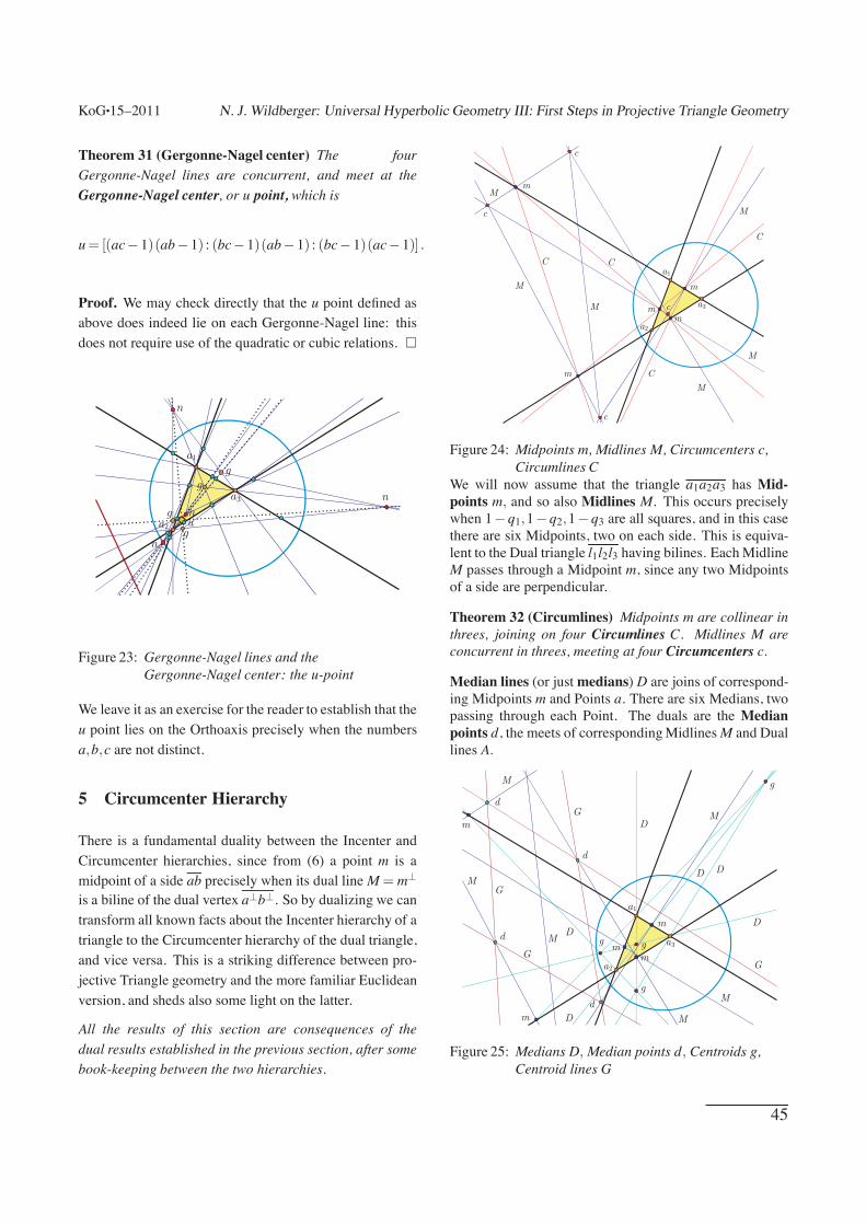
Figure 24: Midpoints m, Midlines M, Circumcenters c,Circumlines C

We will now assume that the triangle a1a2a3 has Mid-points m, and so also Midlines M. This occurs preciselywhen 1−q1,1−q2,1−q3 are all squares, and in this casethere are six Midpoints, two on each side. This is equiva-lent to the Dual triangle l1l2l3 having bilines. Each MidlineM passes through a Midpoint m, since any two Midpointsof a side are perpendicular.

Theorem 32 (Circumlines) Midpoints m are collinear inthrees, joining on four Circumlines C. Midlines M areconcurrent in threes, meeting at four Circumcenters c.

Median lines (or just medians) D are joins of correspond-ing Midpoints m and Points a. There are six Medians, twopassing through each Point. The duals are the Medianpoints d, the meets of corresponding Midlines M and Duallines A.

a

m

g

g g

g

d

d

d

d

G

G

G

G

D

D

D

D

D

Dm

m

m

m

M

M

M

M

M

M

a

a

1

2

3

Figure 25: Medians D, Median points d, Centroids g,Centroid lines G

45


Theorem 33 (Median harmonic conjugates) The twoMedian lines through a vertex of the Triangle are har-monic conjugates with respect to the two Lines of thatvertex.

Theorem 34 (Centroids) The Median lines D are concur-rent in threes, meeting at four Centroid points g. The Me-dian points d are collinear in threes, joining on four Cen-troid lines G.

A Median Thaloid is a Thaloid of a side consisting of twoMedian points, both on a Dual line of the Triangle. Thereare three Median Thaloids.

Theorem 35 (Isostatic points) If two Median Thaloidsmeet at a point r, then the third does too.

Such a common point is an Isostatic point; Figure 26shows the three Median Thaloids as well as two Isostaticpoints: r1 and r2, and their join.

a

r

d

d

d

dD

D

D

DD

A

A

D

ar

a

l1

1

2

1

2

2

3

3

Figure 26: Median Thaloids and Isostatic points r1 and r2

The four Circumlines and the four Centroid lines are cor-responding, since the three Midpoints that join in a Cir-cumline also give rise to the three Median lines passingthrough a particular Centroid line, which is dual to a partic-ular Centroid line. CircumCentroid points are meets ofcorresponding Circumlines and Centroid lines. Circum-Centroid lines are partially analogous to Euler lines, be-ing joins of Circumcenters and Centroids. The next resultshows that the z point might also be called the Euler cen-ter!

Theorem 36 (CircumCentroid axis) The four Circum-Centroid points are collinear, and join on the Z line. Thefour CircumCentroid lines are concurrent, and meet at thez point.

a

a

a

z

g

c

c

Zc

c

gC

G

G

G

GC

C

C

g

g

1

2

3

Figure 27: CircumCentroids, the Z line and the z point

CircumDual points are meets of Circumlines and Duallines. There are twelve CircumDual points, four on eachDual line, three on each Circumline. CircumDual linesare duals of CircumDual points. Tangent lines are joinsof corresponding CircumDual points and Points; there aretwelve. Tangent points are duals of Tangent lines.A Circumcircle is a circle centered at a Circumcenterpassing through one, hence all of the Points. These areshown in Figure 28, with CircumDual points and Tangentlines, which really are tangent to the Circumcircles.

A

A

C

C

C

C

a

a

a

1

2

1

2

3

Figure 28: CircumDuals points, Tangent lines, Circumcir-cles and Sound points

Sound points are meets of Tangent lines and Lines; thereare twelve, three associated to each Circumline. They arealso shown in Figure 28. Sound lines are the duals ofSound points.

46


Theorem 37 (Jay lines) The three Sound points associ-ated to a particular Circumline C join on a Jay line J.

There are four Jay lines, and Jay points j are their du-als. CircumJay points are meets of Circumlines and as-sociated Jay lines; there are four, and CircumJay lines aretheir duals; joins of Circumcenters and Jay points.

A

A

C

B

J

J

Jj

j

J

b

c

c

c

c

C

C

C

a

a

a

l

1

2

1

2

3

3

Figure 29: Jay points and lines, CircumJay points andlines, and the Base center b

Theorem 38 (CircumJay center) The four CircumJaypoints join on the Base axis B. The four CircumJay linesmeet at the Base center b.

Theorem 39 (Wren lines) Sound points associated to dif-ferent Circumlines are collinear in threes, and join on fourWren lines W.

The duals of the Wren lines are Wren points w. To eachWren line we associate the Circumline not associated to theSound points on it. CircumWren points are the meets ofCircumlines and associated Wren lines, and CircumWrenlines are their duals.

Theorem 40 (CircumWren center) The four Circum-Wren points join on the Orthic axis S. The four Circum-Wren lines meet at the Orthostar s.

A

A

CW

S

W

w

w

ws

w

W

W

c

c

c

c

C

C

C

a

a

a

l

1

2

1

2

3

3

Figure 30: Wren points and lines, CircumWren points andlines, and the Orthostar s

A JayWren point is the meet of associated Jay lines andWren lines; there are four. The duals are the JayWrenlines.

Theorem 41 (JayWren center) The four JayWren pointsjoin on the JayWren axis, or the V line. The four JayWrenlines meet at the JayWren center, or v point.

This is a good point to remark that in the projective situa-tion there are remarkable additional constructions, that areavailable at times when midpoints and bilines may not ex-ist, which allow a wide extension of many of the theoremsin this paper. This topic will be developed elsewhere.

A

A

W W

w

w

w

w

W

W

J

J

J

Jj

j

Vv

a

a

a

l

1

2

1

2

3

3

Figure 31: JayWren points and lines, JayWren center v andaxis V

47


6 Bridging between the Incenter and Cir-cumcenter hierarchies

Although we have so far emphasized the complete dualitybetween the Incenter and Circumcenter hierarchies, it isalso the case that there are numerous remarkable connec-tions between the two. We give a brief indication of thiswith three examples, leaving proofs to another occasion.We assume we have a (generic) triangle a1a2a3 with bothBilines and Midpoints (so both hierarchies exist). This is,at least approximately, the situation with our example Tri-angle.

Theorem 42 The JayWren center v, the Gergonne-Nagelcenter u and the Orthocenter h are collinear.

a

v

u

h

a

a

1

2

3

Figure 32: Jay-Wren-Gergonne-Nagel axis

Theorem 43 (InCirc joins/meets) The 16 InCirc joinsjoining the four Incenters i and the four Circumcenters cmeet also four at a time at four InCirc centers r.

a

a

a

i

i

i

i

r

r

r

c

c

c

c

r

1

2

3

3

1

2

L

L

L

Figure 33: InCirc joins and InCirc centers

The four Incenters i, four Circumcenters c and four InCirccenters r form a pleasant symmetrical configuration of 12points.

Theorem 44 (InCentroid joins/meets) The 16 InCen-troid joins joining the four Incenters i and the four Cen-troid points g meet two at a time at 24 InCentroid meetswhich lie, 8 each, on the Lines.

a

a

a

i

i

i

g

gg

g

i

1

2

3

3

12

L

LL

Figure 34: InCentroid lines and meets

An interesting direction is to ponder the implications ofthis work for classical Euclidean triangle geometry. Thereare also many further phenomenon in the projective settingwith no obvious affine/Euclidean parallel, which will bestudied in future papers. The author will shortly post Tri-angle Geometry GSP worksheets on his UNSW website.Hopefully these, together with the formulas and picturesin this paper, will empower and encourage the reader tomake his/her own discoveries!

References

[1] W. BENZ, Classical Geometries in Modern Contexts:Geometry of Real Inner Product Spaces, Birkhauser,Basel, 2007.

[2] O. BOTTEMA, On the medians of a triangle in hyper-bolic geometry, Can. J. Math. 10 (1958), 502–506.

[3] H. BRAUNER, Geometrie Projektiver Raume I, II,Bibliographisches Institut, Mannheim, 1976.

[4] H. S. M. COXETER, Non-Euclidean Geometry, 6thed., Mathematical Association of America, Washing-ton D. C., 1998.

[5] O. DEMIREL and E. SOYTURK, The hyperbolicCarnot theorem in the Poincare disk model of hy-perbolic geometry, Novi Sad J. Math. 38(2) (2008),33–39.

48


[6] M. J. GREENBERG, Euclidean and Non-EuclideanGeometries: Development and History, 4th ed., W.H. Freeman and Co., San Francisco, 2007.

[7] R. HARTSHORNE, Geometry: Euclid and Beyond,Springer, New York, 2000.

[8] N. IVANOV, Arnol’d, the Jacobi Identity and Ortho-centers, Amer. Math. Monthly, 118(1) (2011), 41–65.

[9] C. KIMBERLING, Triangle Centers and Central Tri-angles, vol. 129 Congressus Numerantium, UtilitasMathematica Publishing, Winnepeg, MA, 1998.

[10] C. KIMBERLING, Encyclopedia of Triangle Centers,http://faculty.evansville.edu/ck6/

encyclopedia/ETC.html.

[11] A. PREKOPA and E. MOLNAR, eds., Non-EuclideanGeometries: Janos Bolyai Memorial Volume,Springer, New York, 2005.

[12] N. SONMEZ, A trigonometric proof of the Euler theo-rem in hyperbolic geometry, Algebras Groups Geom.26(1) (2009), 75–79.

[13] A. A. UNGAR, Hyperbolic barycentric coordinates,Aust. J. Math. Anal. Appl. 6(1) (2009), 1–35.

[14] A. A. UNGAR, Hyperbolic Triangle Centers: TheSpecial Relativistic Approach, FTP 166, SpringerDordrecht, 2010.

[15] N. J. WILDBERGER, Divine Proportions: Ratio-nal Trigonometry to Universal Geometry, Wild EggBooks, Sydney, 2005.http://wildegg.com.

[16] N. J. WILDBERGER, Affine and projective metricalgeometry, arXiv: math/0612499v1, 2006, to appear,J. of Geometry.

[17] N. J. WILDBERGER, Chromogeometry and Rela-tivistic Conics, KoG 13 (2009), 43–50.

[18] N. J. WILDBERGER, Universal Hyperbolic Geome-try I: Trigonometry, arXiv: math/0909.1377v1, 2009.

[19] N. J. WILDBERGER, Universal Hyperbolic Geome-try II: A pictorial overview, KoG 14 (2010), 3–24.

[20] N. J. WILDBERGER, UnivHypGeom:http://www.youtube.com/playlist?list=

PL6ACFCC19EA82CA71&feature=plcp

[21] H. E. WOLFE, Introduction to Non-Euclidean Geom-etry, Holt, Rinehart and Winston, New York, 1945.

Norman John Wildberger

School of Mathematics and Statistics UNSW

Sydney 2052 Australia

e-mail: [email protected]

49

universal hyperbolic geometry iii: first steps in projective triangle

Documents