(12) United States PatentBrooks et al.

(54) DECONVOLUTION METHODS ANDSYSTEMS FOR THE MAPPING OFACOUSTIC SOURCES FROM PHASEDMICROPHONE ARRAYS

(75) Inventors: Thomas E Brooks, Seaford, VA (US);William M. Humphreys, Jr., NewportNews, VA (US)

(73) Assignee: The United States of America asrepresented by the Administrator ofthe National Aeronautics and SpaceAdministration, Washington, DC (US)

(*) Notice: Subject to any disclaimer, the term of thispatent is extended or adjusted under 35U.S.C. 154(b) by 1417 days.

This patent is subject to a terminal dis-claimer.

(21) Appl. No.: 11/126,518

(22) Filed: May 10, 2005

(65) Prior Publication Data

US 2006/0256975 Al Nov. 16, 2006

(51) Int. Cl.H04R 3100 (2006.01)

(52) U.S. Cl . ........................... 381/92; 381/91; 381/122;367/118; 367/119

(58) Field of Classification Search ............. 381/91-92,381/56-57, 66, 122; 367/118-119

See application file for complete search history.

(56) References Cited

U.S. PATENT DOCUMENTS

4,741,038 A * 4/1988 Elko etal . ....................381/92

(lo) Patent No.: US 7,783,060 B2(45) Date of Patent: *Aug. 24, 2010

5,500,903 A * 3/1996 Gulli ........................... 381/92

7,269,263 B2 * 9/2007 Dedieu et al . ................. 381/92

OTHER PUBLICATIONS

Thomas F. Brooks, "A Deconvolution Approach for the Mapping ofAcoustic Sources (DAMAS) Determined from Phased MicrophoneArrays," 10th AIAA/CEAS Aeroacoustics Conference, AIAA(Manchester, UK), (May 10, 2004).

* cited by examiner

Primary Examiner Xu MeiAssistant Examiner DislerPaul(74) Attorney, Agent, or Firm Helen M. Galus

(57) ABSTRACT

A method and system for mapping acoustic sources deter-mined from a phased microphone array. A plurality of micro-phones are arranged in an optimized grid pattern including aplurality of grid locations thereof. A linear configuration of Nequations and N unknowns can be formed by accounting fora reciprocal influence of one or more beamforming charac-teristics thereof at varying grid locations among the pluralityof grid locations. A full-rank equation derived from the linearconfiguration of N equations and N unknowns can then beiteratively determined. A full-rank can be attained by thesolution requirement of the positivity constraint equivalent tothe physical assumption of statically independent noisesources at each N location. An optimized noise source distri-bution is then generated over an identified aeroacousticsource region associated with the phased microphone array inorder to compile an output presentation thereof, therebyremoving the beamforming characteristics from the resultingoutput presentation.

20 Claims, 26 Drawing Sheets

U.S. Patent Aug. 24, 2010 Sheet 1 of 26 US 7,783,060 B2

LJL

cc N

6ftaft

LL

U.S. Patent Aug. 24, 2010 Sheet 2 of 26

US 7,783,060 B2

1/1 •

N ! • • •

oIt Nc l

U.S. Patent Aug. 24, 2010 Sheet 3 of 26 US 7,783,060 B2

dB 60 70 80 9.0 1.00

300

STD Beamforming

99

W^CO

DAMAS, 1 iteration- }-Y t

— i1 . ^_,. .^'-- L Yeti 1{

1 —"1 l..* .

DAMAS; 1000 Iterations r

tY-r- frt ^-'^' ^ ^- {—{-^ r ^ u^wi ^ ^ ' t ^ i

L t; L ^ I `'

f + t F +'s ( t 4

n ++ - +^`F '77-7 71.

r ^ ^7=-.7t

it — £ i .y1 J «{^ j..{. ^ . }.,

D4 AMAS; 5000 iterations; it

TS

t 1 J t !

{^ k + t t t {^ r {. } i t. f

-20 0 20

60

50

40

C30

O

20O

60

V50

40

30

20

Spanwise location (in)

FIG. 3

U.S. Patent

Aug. 24, 2010 Sheet 4 of 26 US 7,783,060 B2

Q

^y.-r—I....-..^+•-f..F- t^^..Sk,. M^-^ ^

ti^-^^ti^^^•b-^'-^•^'^_^^. ^..3^-tr-1M3•ir..,^.N ^.. wi

..1 r l j:...r{^-t

r-.-...rt.. ^^^.^L._^-•—:THr 1._}_.^..^-.^i—f-1'^1... j_T.^.. ^'ii_ 1...:..:..e..^i..`_i_.',^'....1. '''^:.

ti

..^... +-} ". G ^._:-i } -^ *- f^-T.' ^'^-^ -^-••r-rl-^^ r:-^ :^I-.^>;-^-ice 4-^-e-si-

a4-

te

{`?' ^ ^ ^ mil•

C

Wf .g. 0) o .o0'

N

O

Oaft

C

aoN

n

N LLC.

co

0

E

m

NU^

i

to W) N(ui) uoileOOI aslemPJ04:D

U.S. Patent

Aug. 24, 2010 Sheet 5 of 26 US 7,783,060 B2

500

60

50

40

c30

O

0 2041

60

O050

40

30

20

STD Beamforming

fG ^• `^ G^ ^C^ ^`^ ^

I3

C)

& ^; 097) -.as

^_CO' .

DAMAS, 1 Iter^¢a¢ tio^n

p j ,, ; 4

Lj t 7 3h dye P +^RI^4-I f tr yt3#,^

r ,

, s iT t

- F I L S f «-1 a+_

t r

L S,>j

{ f^f !! r.

.20 0 f'' 20 6^

DAMAS; 1,0001te"r 1-ty

x . I " — T7 tI `yi

+^ rj1 tom!

x

s t r ±1-7—TTtt

^.

!19

DAM terations

'' ) " t s -jT fir V-+ z

9t 11 ,r ! 7 7' j J1 iT^

^ ^ 7.f i a rt

Y"r

L;.T '., It ^t^^V, ^

^. St

tr ^^Y.

-20 0 20S panwise location (in)

FIG. 5

40

30c0

200

X16..

113

.. i10^

U.S. Patent Aug. 24, 2010 Sheet 6 of 26 US 7,783,060 B2

600

NIX

STD Beamforming

607 109 r 1 10

dB 60 70 80 90 100

:DAMAS 1000Iterateonsl ``tt=

NAG"

• I. i ^ rf^ ^^ ^1. I . f -i ^^,lt i

DAMAS, .'lrlteration .; - ;1 1{ ++ 1

..,- air 1 ^: (. y^^ ' f ; +.

1 ^IF[ t N6w'/!1'^ i1f^l^tMbE6 MYlf..i .. .-1[^,a, ^n^ISS1iYaa.b.T1 sGa.4Wa n y^L"^^.. ._..- sltrR9xaYMtf^Y1iY^M ^aawxw3at^E^?_ ^..

r DAMAS; 50:0:© Iterations L

T 1.^ t•t _^ rF p;^ ^,^+:^ . -3-711 1 1_.q i ....^ i .. Y 1 n ^E yy r f.n 1 a

-,

'T akii ^, Sy _ ^i 3^ {ia sft . `- ter ,iR7f1L il ^

.iww y'1^nic^iti, ^tln ! 1 Ma

^' •LI/py ^ylllnA !t A., n

a^-3 60

v 5040

20

30_ '^.;rz8^c7^ret^airaiaitcairif►>t':^'wi^ew^ ..:

-20 0 20 -2O 0 20Spanwise location (in)

FIG. 6

N }'00

o AN G

tpQ.co

Nn

6

LL

W LO qq* M N(Ul) U01je3ol OSIMPAoy o

U.S. Patent Aug. 24, 2010 Sheet 7 of 26 US 7,783,060 B2

is ^kN,^.. ♦: :'

_ iii r

N

0

OC'.9

402

Em

W

V/

- ^.

o ^.

co

CN QD ,.to't p O .r p

ti^

^ OD"

.^^ A / e

O

0N

U.S. Patent

Aug. 24, 2010

Sheet 8 of 26

US 7,783,060 B2

800

DAMAS, ! .Iteration: ^ --------,-i' += k, ^,^^;

l i r ,.:i.aq xkr`w^ +yy^^{{•- NR i{y.w.^[wr ^y n^ub -„

40 iksF.Ra= RC II{z4gY, .^ ai, 7i4k7bP.

AFRE3^^11k^t 11 N!XIaRMNrMII,®_M^ Rk7R

F #6M «^MP^gR^it MNyi^ IM LM4N #

4 17

' F "..--1..`..'.• '; }-',.+_"=".''iC'.-rye -r^y^'

LU

U 10

STD Beamforming

60 104

tl50

O 0^

FOV

W.3 60

0v 50

30

20

DArWAS 1'.00.0.Ater`atiorisFr

..t' "( {r "°}}p`-r

t }.`?" t 1.I j r '! { 1`

r ^i7r.N MyTAiW.`''+•NC:Y,Y,^N

}*^-.11

DAMAS; .5600-,Iterations , °;f '... ;-,-^-'^,^ t.="{.^-''+T^.•'i:I.'=^".-s:-+iii«-`t -^

wir. `+ t 1OT

, I ; .w T_

e^^ i 1 } '^'1. [ !^^

-20S panwise location (in)

FIG. 8

U.S. Patent

Aug. 24, 2010 Sheet 9 of 26 US 7,783,060 B2

900

NIWdB 60 70 80 90 100

60

50

40

c 30

20O

.N 60

0 50V

40

30

20

4J,DAMAS '9..000 Iterations::::­7I

.i .i. ti._...y.ir..

^yV a02

4 d i

k'rL 3I[I B ^ ;^ ::a rw }' i I *". x;i- 1 :"

....., «y.

if`t..^' J 3-}'m

^DAMAS 1000, teratioris= w^ 1,:

;die-o:2s}:.1.:t i. tai•$; 1'^}. .; ^. ^ 14^s. i li^ - '7: :: 'jt

.}n ti ^.. ^^.iY ..p a ems'; -1 PI]YS }'r-t

mar' . 1 :•11,^ J . IT `'.s.: .

iffilgal- Olt j

.20 0 20

rDAMAS.,l,1_ 000jtdedtions

.-3 c.. 11 dlµ e4•-^^.,L^. ^...yy.^Y

2-q' `-{-r.^..4t+..

Ti

i-,-. rf a - ^ •r-^.**-'•r^-r{^ 'M•-^ ^.:.._'+^7''.

.

^ f-""•^.l.Tl.^i.Al.i'.

".

•

.y{

`DAMAS-, 1OOO Iterations =

«\ I a iuy- r=ancid

^ °• ^rF 1' ' +.^-:n ill t

3,Zt'-r-t i1t ^^• ^ ^-i--^^^"^Fs

4T I

rl

^ I' -'+ : ^ ps r ^ r t } T L^^-4 ^ r t ^ ^ Ig-' 4•"^ ':^Il rr i

-20 0 20Spanw" location (in)

FIG. 9

U.S. Patent Aug. 24, 2010 Sheet 10 of 26 US 7,783,060 B2

a00Q^^o

00

0 ^ q ^` qto^! er o

q o q

0cp q to •-

cu co _ 3 OLL o N o0:

v V-

^O No z0C N

Of o O ^O

II ^

0 0^ q N( O O ^ r

^ q Aclq p I

I I

OO

U.S. Patent Aug. 24, 2010

aM

00

Sheet 11 of 26

US 7,783,060 B2

a^0

Vft

6%oftUft

N0r

00rr

N

ftaft

UL

rr

U.S. Patent Aug. 24, 2010 Sheet 12 of 26

US 7,783,060 B2

co co C* OD 00 00a LO mot' M N %—

rn

0

OOO

-I'Lu I'^......... .

A, LLJ

CC'LL

-,Cr

no mil-"_1

58

to

CD

2c0

U?

0

in

CLw

0C%kl

010

110 CD LO

(Ul) UOReDol OSIMP1043

U)

/ .00-

LO.

r

Y !

0

0.r

0

NLn 3

c

CL

0

am

Ew

m0

i3 ( I

r-

3 r^

}}

TAT

C

W

O00r-

Q

a0

n•

C^

U

U.S. Patent Aug. 24, 2010 Sheet 13 of 26 US 7,783,060 B2

0 C> M

C>

1, IT

L

o^MW oqlqt itM

(Ul) u04e301 asimpiouc)

'^'^fr`+Sa.Y _ >._.+.1^s3-: ..^y.L °43 - . •; ,^ ..;i x" ^ .y'^e'..c

"^ .,R t.^_

--O_w-

LU1.^ V

^i^

•O

La

QO

craQ

0D

U.S. Patent Aug. 24, 2010 Sheet 14 of 26

US 7,783,060 B2

00 co 00 00 co co-^ U,) qt CO N

_U

LO ^ n

---0 rna^

1 Cfl. 11 N - 1

.Q

LOE

CDm

c /f

^ 4 ^

(UI) U014coOl asimp o4 c)

C3

rte\

i^

,oIn y

O

3ULm

CLw

0

LOYr

L /

4 -4

j

SAWry

7Z

D

+ L

;_t4

0

Bl

404040

Lc)

CD

dO^

%ftw

c0

0(DU)

Ln

CLU)

tr)VAft

n

ftftft

LL

IU-)

U.S. Patent Aug. 24, 2010 Sheet 15 of 26 US 7,783,060 B2

0 ad' a a a

J0.E cqti

LO r-;_

V.

Q

to 0 Ln

LOV- (Ul) U01le0ol OSIMPJOLID

T

U.S. Patent Aug. 24, 2010

Sheet 16 of 26 US 7,783,060 B2

^oo

1604

7300

---16021014 SADA

_J-__ ___ ^41606

O= 9o0

01070

1240

1410

I rTE ^rI ^ ^

I 1008 Ir.

od, I.I I

LE. Grit

1010

Flow

1001

Nozzle1012

FIG. 16

zp

Cl) ^^^ v

ry \ M

Q 6Cl)

M \

d `1

r>

dM:e M i't,'r,^i

p 1ti O V

m

k-ol ^

M

f co I ,

1 / a ^ ^ ^ A^^' \a cn^

MQ ^

\cr b N

M

^`,a d^ poi d OQv^

O v/

d J Pn a .- 2 4, A6 N

N pry Oa ).'T J

C

CO

OON

(0a

DY

C

O

D

N

coQ

DM

C6 V.4 a

O^ 1

//a u^ ^ ,n

rm v

^1

O(p

11 P

1 ^ /^. ^ \^ crn

a

'm v

r `^^J

Cl)

a

e m

^\ d

On

0n

CCO

O

N

caQcn

EZ

C

CO

O

N.0

(6a

U.S. Patent

Aug. 24, 2010

Sheet 17 of 26

US 7,783,060 B2

00

v v o O Ofa 1A V m N

( • ui) uoiJeooI asimpa043O o O O Ow 10 Q M N

(ui) uoi^eDOI asinnpaoy0

t0 49 ^ ch N

M N Nt M N

( • w) suoileool aslmpjoy3

(-u i ) suo11e301 8sinnpA040

C 60

C50

CuUOaD 4UCn

.3:

20 30O

U20

36

26

16

6

-4

U.S. Patent

60

0 50c^U

—O 40

300L

..0U 20

Aug. 24, 2010 Sheet 18 of 26 US 7,783,060 B2

Ird

J'13 - 3.15 kHz

-TE Int Area I -

-- - - - - -e Ix

x^^4 4x aa!ta.. s, b.,^`ydt,<3d*'^ :^ " h^ ..

Spanwise location (in.)1800

dB

40

30

20

10

0

1802

Spanwise location (in.)

FIG. 18(a)

60

0 50U

40C/

-2300()20

_i.. S;e...._ ►Sll^tit .:.<^.:r,.`.:rt.+r"^63%^ ,: :J-^ ..12.5 kHz icy

rr.....x.._.

. 1 ' i^'^ `J^'.'.:^'. r, A::t^Y^ Rr5{^`';%x3^c%h`^.?^^^:3s:.:;: ^Y,.ti^..r..,_^%r... :F'i:^..F.. ::^^Y L..r, ,

w.' •,-tom .'r" .+:{..{{.;:;. .. . .

..

... $ ^ff'S^atw^^•tlea ^°rs+z

i ,R W' `xd^ ,^.•.f.3kyrs•t't 1A M7P 1 '

Yk.

rlye

' k J.^T t

^ t ^^ i ^^= k ^ ^^L C^ +^^yypp V^

^•NtC^ y+^ R 1 ^YK.NIil^9 r'a.?^.,.. _ ^

R 31 [! RKr ,. i^ +N {ry. ^1' \ A . . ;^,f^!l:i^.^{1^}pg^.^ 'S Q ^^iy^}`Q^FSSnY .^ tEl]iiC;'_^^ F

r:VxM4^' ^ ^!t .1`4`^1 ^

"L.^^^i^^.'^^<^^

7^ ^ ?Keitr^d^^ri.13 ^

-5: ']^F•4^M^^R. ba.•„^

^^^.p'^7,5^^ ^^'^^ ^ 1^^..ar ^'^.{y 7J. ^Td^^ ^Nw ;4 SAS y^^^

7^.^'^)1ry.t,"'"•^'^ d., i l^ri i

' 3'a^ys"^FF .,y .9{'F= :'1t S."ui 4 k ^fFP y^e^^

,,,T7

!,F... L ^ ^.. ^ i F ^

44^4'a}+Yf XAF^ ^ a •f ^^ ^'ql

:::x::^^ ^... t r ^' }y„'

`' y}y^fl^,.

fta^^, ^ `i

^^• ^ -^-c^^`^",^-^ ^ ^ r ^

.}.F. `4 Z .. 1 Y'^+y^^ 4 'V k a^ I' L'{.^6M 7 y^ty.^^

rr-v

^A}

tom

^} .^./11^ ^`+ M1

rtnxar^ a^p7 yr• ^ .. .per•<r ... .c^ ^',^ ^G^°'FS.+^..Y&'9 f^^s^S ,•'A.::^:^'^c1'Ee ' -,T^§!„ ^ _ 2^ 'is<•Sj

<. ^.•^^` ra

^^i.l,.' Lam; ri^k^yr^... ,^-. t^^`^ "x£, 1K: k '.t r ... .

36

26

16

6

-4

f v3 0 kHz , yg ,.. rkY..ru

'33R.g^

R^Att s ad a ir u _ to U ^^z . 's3L ., `'' g YCt C$F} ass,. y

Y ^

" S I t 7 t S:t 21

1^ gu

S rH

^^

.RI r.Y

II^. NCr7

tm,"

9 I` th

^^,, aF..^`}{♦

qy^i

i.C^4

RpY^, 4ar, C ^. -x ^C'+1k'^¢"'^1

iyT ^^`L` 4 F ^YTT'i£

C. gg^'^^ ^(

w a S RCCS,,4""r^'^ rt .+^,y^ ^7f ^`d ^^..r ^ +'r ^t+srx "^ ^^t ^Yfis,

r '..Y.^^jM1ykY+'C^I{^

FX'^6'Y i" ` ^'4`'YTtF .j{ ^4r„ fit: Y'^'df m F3. rO^J^.^tu3

l5^

Zy53+b

t

{T{ °§2r+ 1+5'. ^,^ t ky^ Q. w`e x!e'M'e^1'kff.

^^,41^e^^,qr: ..,

l:^:a.'sF tk— bp,..'r

y

`r!,

^,3 '+> e^ R fY1..i^3 k>^i GtJF9'i^^^^i.•^''.":SIar.&^ ^"^

azr'..9"'Y f r ^n., C '^' i^A..C y{yew ...J[S*i ^^,a.

tgs ^fi1 ,

60

50P

CO

40

-a 300

U 20

40

30

20

10

0

U.S. Patent

Aug. 24, 2010 Sheet 19 of 26 US 7,783,060 B2

Spanwise location (in.)

1804

-20 0 20Spanwise location (in.)

FIG. 18(b)

1806

co

:

;Ak Q

c0

D 0(U

C:wCLcn

D

c0

.24)U)

CLU)

OC0

0

coi=U)

CO

Lf)

LOL^u

LoF—

fj

0

w

1 0 1 41

1

51

0

A15 11;

1coC^

co

N

ftAkft

LL

U.S. Patent

Aug. 24, 2010

Sheet 20 of 26

US 7,783,060 B2

co

C)vs

Iza Q1 CD Qto

U,I

N(Ul) UOIIL-001 BSIMPAOLIO

GD C2 C2 0 0(D Ln v m C4

(-Ul) U0112001 9SIMP1040C)

N

0 0 CD CDLO IT m C14

(Ul) u0pool 0SIMPA040

C),CD Q CD CDto to IV m C14

(-Ul) U011-nol 0slmpj0q0

dB40

30

20

10

0

2000

Spanwise location (in.)

2004

z

^`^ism,Y£iA 4hA'sp+£&W.'.^" a'9Y'L'3.: 1Ar4. i ^.. 5^.dwA ^,h,

k^4F.hy^

^YA+ '*.rty,by fl "^

s_o51 ^s tad^ 5

,.i ^^ ^,"'S J lh^I1V,. "'a Rf`:S .SrSC.X _ lkq ..

a,r^lr^ :a rc ^ r 1, f, - ,l!L

.._S

^.^: ,... _Q r - ^ : ^W'W:.SI ' a°t;[.s ^^. 1:: IR K}.'L: ^:: ^L ,I(FY:'; ffi'/.^ SiCS.;:A' L'

60C

0 50czU

40

-o30

i

020

36

26

16

6

-4

U.S. Patent Aug. 24, 2010 Sheet 21 of 26 US 7,783,060 B2

60

0 50COU—° 40a^

_0300C-

U 20

Spanwise location (in.)

FIG. 20(a)

:../ = 12.5 hflz.J //3

.. ,. ...

d3A.

ti ^}}Ky

t' aL'Y. ^ ^'' B.a'P3 .I.T.. ^I^°iY

rt h ^ f7.'-3^a'" -°'^ f'1 +L^1E 7,^°f,tic.-: .'.1.i:3W^&itiSFiS CF^ ^L`sr

x E$.' &"w t^', ^ pa i

f+f*,`^lkst .^ 's

Tfsd6 d^ 3 „Sw''^ ,.,,^^''

'$ s °u.a Z"a Ea^ &' 'k.' t ... az

^R fJx?^ S^^{*'t ^.^ K 1 Ts ^`a '2^7,i. r ha^n R`^

r ^' 2^^s+"w4^fr^.^

}.!^

£ i'1§ ^'St .' ka "s ku!'-C "'^^^.F.e

a 4^

r tr fr + FCtnY.9S

^ }Yw 'S-rM './.^W^S.

.ryYr f^.5. 5

iy'^' ^'w

'3•'Yr ^^°^^^aar x , a

K `^ :: F rM K ^. M 3 .i 1` .i. ,K.S^ 3 ti^ L .Rw .c,e swwtt l.r'i. Pl-d'3' v ilz'ES 7r ^,'aS.`r^a f° 1 +fJ,.. _.ua,•Y ^, -'3^ ^*i^F%}

wa

k2. l":„.;.5 .. '...t t.. - 5 .m - ' Iq ^.V -Y.. 1 `T• i .. .a^ . i.. .s`8 nr n;:FYG. ^:^C

2006

36

qtr; 26TS!^(L^

16.z.i

6v3F"rT-

-4

60C

0 50

U—^° 40^

p 300020

U.S. Patent

Aug. 24, 2010 Sheet 22 of 26 US 7,783,060 B2

Spanwise location (in.)

J,, 20 kHzf^ r^^^w e

0 50

0 40 n rr i'y'7", L'#.dti%3 Pfi,a t+-9^a ¢ qa

W .'3 ^ ^s-.. ^ Kam` '^a a^^.a ^^^a^,;,J Fes' C'^ s. "h ^t.

P.^

^ ^^' S°#s!^ y ti ^ iW I',. 4s EY.` ^s^hy,^'^i+, ^•^'.{^^i5'•^.x^

VV 0 Ci ^. s s^, Z^t g r ;

'big 0.-y^ ^R ^ ^} se w F....*'^'vt^,si^.,AF ^^rrxi^ 7 cs^^-. 'ikA•^ ,

Y.p 1l ^'P'F p Ky g 4 G; S .`

dit

t^ «!a^' +k5 '+1 ° . a^ va 3d ^. y 4{szC`tti1 soh r.a ^s +,a _^3.

O +" E9 ^' t^ cn68 T 154 +&^a r

'La+Y: '' sl°,ffi°" Y^ iGt `^ WR

^ 'Y- (.& Yi# C f''''P3 4 ^.,1"!L, u3 S3 IY 'F^ .

d

^e.^.yiP.*^^.'99r4 ak'i.^•a,^,akY^.A'+^+'A:£d ^ uT.^1^Sr^^ 9i2t1 ^$3

' :na'A. < .Fr. .:.-s.P=.. 7^.:a:seYry: s.-- • kl^r7'.' ..k N'^%ffi -..t w.r ^:4 ..:.. C ...,+: .ak ^.+^+'m^1Gi '7dt':^

-20 0 20Spanwise location (in.)

FIG. 20(b)

40

30

20

10

0

00

N

Q O

42

C. Q.

W W

O OLr

LY LA U) W 4)

a ^JFW- W W

3 3 U)toJ }^-

CL^

QQ aegg

U)QQ

U)

Q d cl ^ Qp 00Q Qi^wIXto CO) co(n 00

I

^ CD in(GP)'ldS

'd MO00

a ^

^ 4

s

7 O

O Nr ^^ NC

rv^^

LLU.

V)O

U.S. Patent Aug. 24, 2010 Sheet 23 of 26

US 7,783,060 B2

NN

n

kftft

LL

U.S. Patent Aug. 24, 2010 Sheet 24 of 26 US 7,783,060 B2

§ o

a

mil o ^ oa

R >%i

co

d0v

U.S. Patent Aug. 24, 2010 Sheet 25 of 26 US 7,783,060 B2

602 Q

50

40

30

020

0as

' 60

OU 50 gt

dB52

40 :s32

42

rs 22

30 1 2

20

-20 0 20Spanwise location (in)

='r`.,-mow 2:7:: ^- M rI,'!

^e ^

. .^. DR QAMIAS

^^

Y Fib

t

^'^^7L^w

-Slat int. Are^a^,_ ^^cr ^ 41i

tiE

FIG. 23

U.S. Patent Aug. 24, 2010 Sheet 26 of 26 US 7,783,060 B2

24

60

50

40

30

0

20

0

60

O

DR Beaiwor,'^^-,--38----- 11

v,.i z - 39

0

4

37' 35

7. aMw- 0,,Zql 1, ' . .)

ANXI I - jrl Wit

dB4So 5

94

J-4F, pF,

r. FRI,

35

40 25

15

kzIC44 00Ov

5

20

VkIJk., w X ^!ill I t -QR^-11 K4 s.

304NT............

I J*.,

-20

0 20Spanwise location (in)

FIG. 24

US 7,783,060 B21

DECONVOLUTION METHODS ANDSYSTEMS FOR THE MAPPING OF

ACOUSTIC SOURCES FROM PHASEDMICROPHONE ARRAYS

TECHNICAL FIELD

Embodiments are generally related to phased microphonearrays. Embodiments are also related to devices and compo-nents utilized in wind tunnel and aeroacoustic testing.Embodiments additionally relate to aeroacoustic tools uti-lized for airframe noise calculations. Embodiments alsorelate to any vehicle or equipment, either stationary or inmotion, where noise location and intensity are desired to bedetermined.

BACKGROUND OF THE INVENTION

Wind tunnel tests can be conducted utilizing phased micro-phone arrays. A phased microphone array is typically config-ured as a group of microphones arranged in an optimizedpattern. The signals from each microphone can be sampledand then processed in the frequency domain. The relativephase differences seen at each microphone determines wherenoise sources are located. The amplification capability of thearray allows detection of noise sources well below the back-ground noise level. This makes microphone arrays particu-larly useful for wind tunnel evaluations of airframe noisesince, in most cases, the noise produced by wings, flaps, strutsand landing gear models will be lower than that of the windtunnel environment.

The use of phased arrays of microphones in the study ofaeroacoustic sources has increased significantly in recentyears, particularly since the mid 1990's. The popularity ofphased arrays is due in large part to the apparent clarity ofarray-processed results, which can reveal noise source distri-butions associated with, for example, wind tunnel models andfull-scale aircraft. Properly utilized, such arrays are powerfultools that can extract noise source radiation information incircumstances where other measurement techniques may fail.Presentations of array measurements of aeroacoustic noisesources, however, can lend themselves to a great deal ofuncertainty during interpretation. Proper interpretationrequires knowledge of the principles of phased arrays andprocessing methodology. Even then, because of the complex-ity, misinterpretations of actual source distributions (and sub-sequent misdirection of engineering efforts) are highly likely.

Prior to the mid 1980's, processing of array microphonesignals as a result of aeroacoustic studies involved time delayshifting of signals and summing in order to strengthen con-tributions from, and thus "focus" on, chosen locations oversurfaces or positions in the flow field. Over the years, withgreat advances in computers, this basic "delay and sum"processing approach has been replaced by "classical beam-forming" approaches involving spectral processing to formcross spectral matrices (CSM) and phase shifting usingincreasingly large array element numbers. Such advanceshave greatly increased productivity and processing flexibility,but have not changed at all the interpretation complexity ofthe processed array results.

Some aeroacoustic testing has involved the goal of forminga quantitative definition of different airframe noise sourcesspectra and directivity. Such a goal has been achieved witharrays in a rather straight-forward manner for the localizedintense source of flap edge noise. For precise source localiza-tion, however, Coherent Output Power (COP) methods can beutilized by incorporating unsteady surface pressure measure-

2ments along with the array. Quantitative measurements fordistributed sources of slat noise have been achieved utilizingan array and specially tailored weighting functions thatmatched array beampatterns with knowledge of the line

5 source type distribution for slat noise. Similar measurementsfor distributed trailing edge noise and leading edge noise(e.g., due in this case to grit boundary layer tripping) havebeen performed along with special COP methodologiesinvolving microphone groups.

10 A number of efforts have been made at analyzing anddeveloping more effective array processing methodologies inorder to more readily extract source information. Severalefforts include those that better account for array resolution,ray path coherence loss, and source distribution coherence

15 and for test rig reflections. In a simulation study of methodsfor improving array output, particularly for suppressing sidelobe contamination, several beamforming techniques havebeen examined, including a cross spectral matrix (CSM) ele-ment weighting approach, a robust adaptive beamforming,

20 and a CLEAN algorithm. The CLEAN algorithm is a decon-volution technique that was first implemented in the contextof radio astronomy.

The CSM weighting approach reduces side lobes com-pared to classical beamforming with some overall improve-

25 ment in main beam pattern resolution. The results for theadaptive beam former, used with a specific constant added tothe CSM matrix diagonal to avoid instability problems, havebeen encouraging. The CLEAN algorithm has been found topossess the best overall performance for the simulated beam-

so forming exercise. The CLEAN algorithmhas also been exam-ined in association with a related algorithm referred to asRELAX, utilizing experimental array calibration data for ano-flow condition.

35 The result of such studies involves a mixed success inseparating out sources. In other studies, using the same data,two robust adaptive beamforming methods have been exam-ined and found to be capable of providing sharp beam widthsand low side lobes. It should be mentioned that the above

40 methods, although perhaps offering promise, have not pro-duced quantitatively accurate source amplitudes and distribu-tions for real test cases. In the CLEAN methodology in par-ticular, questions have been raised with regard to thepracticality of the algorithm for arrays in reflective wind

45 tunnel environments.A method that has shown promise with wind tunnel aeroa-

coustic data is the Spectral Estimation Method (SEM). SEMrequires that the measured CSM of the array be compared toa simulated CSM constructed by defining distributions of

50 compact patches of sources (i.e., or source areas) over achosen aeroacoustic region of interest. The differencebetween the two CSM's can be minimized utilizing a Conju-gate Gradient Method. The application of positivity con-straints on the source solutions had been found to be difficult.

55 The resultant source distributions for the airframe noise casesexamined are regarded as being feasible and realistic,although not unique.

As a consequence of the drawbacks associated with theforegoing methods and approaches, an effort has been made

60 to develop a complete deconvolution approach for the map-ping of acoustic sources to demystify two-dimensional andthree-dimensional array results, to reduce misinterpretation,and to more accurately quantify position and strength ofaeroacoustic sources. Traditional presentations of array

65 results involve mapping (e.g., contour plotting) of array out-put over spatial regions. These maps do not truly representnoise source distributions, but ones that are convolved with

US 7,783,060 B23

the array response functions, which depend on array geom-etry, size (i.e., with respect to source position and distribu-tions), and frequency.

The deconvolution methodology described in greater detailherein therefore can employ these processed results (e.g.,array output at grid points) over the survey regions and theassociated array beamforming characteristics (i.e., relatingthe reciprocal influence of the different grid point locations)over the same regions where the array's outputs are measured.A linear system of "N" (i.e., number of grid points in region)equations and "N" unknowns is created. These equations aresolved in a straight-forward iteration approach. The end resultof this effort is a unique robust deconvolution approachdesigned to determine the "true" noise source distributionover an aeroacoustic source region to replace the "classicalbeam formed" distributions. Example applications includeideal point and line noise source cases, as well as conforma-tion with well documented experimental airframe noise stud-ies of wing trailing and leading edge noise, slat noise, and flapedge/flap cove noise.

BRIEF SUMMARY

The following summary is provided to facilitate an under-standing of some of the innovative features unique to theembodiments disclosed and is not intended to be a fulldescription. A full appreciation of the various aspects of theembodiments can be gained by taking the entire specification,claims, drawings, and abstract as a whole.

It is, therefore, one aspect of the present invention to pro-vide for a method and system for mapping acoustic sourcesdetermined from microphone arrays.

It is another aspect of the present invention to provide for a"Deconvolution Approach for the Mapping of AcousticSources" (DAMAS) determined from phased microphonearrays.

It is yet a further aspect of the present invention to providefor improved devices and components utilized in wind tunneland aeroacoustic testing.

It is also an aspect of the present invention to provide foraeroacoustic tools utilized for airframe noise calculations.

The aforementioned aspects and other objectives andadvantages can now be achieved as described herein. Amethod and system for mapping acoustic sources determinedfrom a phased microphone array, comprising a plurality ofmicrophones arranged in an optimized grid pattern includinga plurality of grid locations thereof. A linear configuration ofN equations and N unknowns can be formed by accountingfor a reciprocal influence of one or more beamforming char-acteristics thereof at varying grid locations among the plural-ity of grid locations. One or more full-rank equations amongthe linear configuration of N equations and N unknowns canthen be iteratively determined. The full-rank can be attainedby the solution requirement of the positivity constraintequivalent to the physical assumption of statically indepen-dent noise sources at each N location. An optimized noisesource distribution is then generated over an identified aeroa-coustic source region associated with the phased microphonearray in order to compile an output presentation thereof, inresponse to iteratively determining at least one full-rankequation among the linear configuration of N equations and Nunknowns, thereby removing the beamforming characteris-tics from the resulting output presentation.

BRIEF DESCRIPTION OF THE DRAWINGS

The accompanying figures, in which like reference numer-als refer to identical or functionally-similar elements

4throughout the separate views and which are incorporated inand form a part of the specification, further illustrate theembodiments and, together with the detailed description,serve to explain the embodiments disclosed herein.

5 FIG.1 illustrates an open jet configuration system whereinan array of microphones is indicated as out of flow and ascanning plane thereof positioned over an aeroacousticsource region, in accordance with one embodiment;

FIG. 2 illustrates a system including key geometric param-10 eters of an array of microphones and a source scanning plane,

in accordance with an embodiment;FIG. 3 illustrates a graphical representation of array output

based on standard processing methodologies, wherein fre-quency is equal to 10 kHz and Ax/B is generally equivalent to

15 0.083 in accordance with one embodiment;FIG. 4 illustrates a graphical representation of array output

based on standard processing methodologies, wherein fre-quency is equal to 20 kHz and Ax/B is generally equivalent to0.167 in accordance with one embodiment;

20 FIG. 5 illustrates a graphical representation of array outputbased on standard processing methodologies, wherein fre-quency is equal to 30 kHz and Ax/B is generally equivalent to0.25 in accordance with one embodiment;

FIG. 6 illustrates a graphical representation of array output25 based on standard processing methodologies, wherein fre-

quency is equal to 10 kHz and Ax/B is generally equivalent to0.083 in accordance with an alternative embodiment;

FIG. 7 illustrates a graphical representation of array outputbased on standard processing methodologies, wherein fre-

30 quency is equal to 20 kHz and Ax/B is generally equivalent to0.167 in accordance with an alternative embodiment;

FIG. 8 illustrates a graphical representation of array outputbased on standard processing methodologies, wherein fre-quency is equal to 30 kHz and Ax/B is generally equivalent to

35 0.25 in accordance with an alternative embodiment;FIG. 9 illustrates a graphical representation of spatial alias-

ing with point source and image shifted between grid points inaccordance with an alternative embodiment;

FIG. 10 illustrates a configuration of a noise flap from a flap4o

edge to an SADA, in accordance with an alternative embodi-ment;

FIG. 11 illustrates an open end of a calibrator source posi-tioned next to the flap edge depicted in FIG. 10, in accordance

45 with an alternative embodiment;FIG. 12 illustrates a graphical representation of calibrator

source test data wherein M-0 with an integrated level of 62.8dB and a DAMAS of 62.9 dB, in accordance with an alterna-tive embodiment;

50 FIG. 13 illustrates a graphical representation of calibratorsource test data wherein M-0.17, with an integrated level of58.1 dB and a DAMAS of 57.3 dB, in accordance with analternative embodiment;

FIG. 14 illustrates a graphical representation of a calibrator

55 source test, wherein M-0 with an integrated level of 62.2 dBand a DAMAS of 61.6 dB, in accordance with an alternativeembodiment;

FIG. 15 illustrates a graphical representation of a calibratorsource test, wherein M=0.17 with an integrated level of 57.9

60 dB and a DAMAS of 56.9, in accordance with an alternativeembodiment;

FIG. 16 illustrates a configuration of a test set-up for TEand LE noise testing, in accordance with an alternativeembodiment;

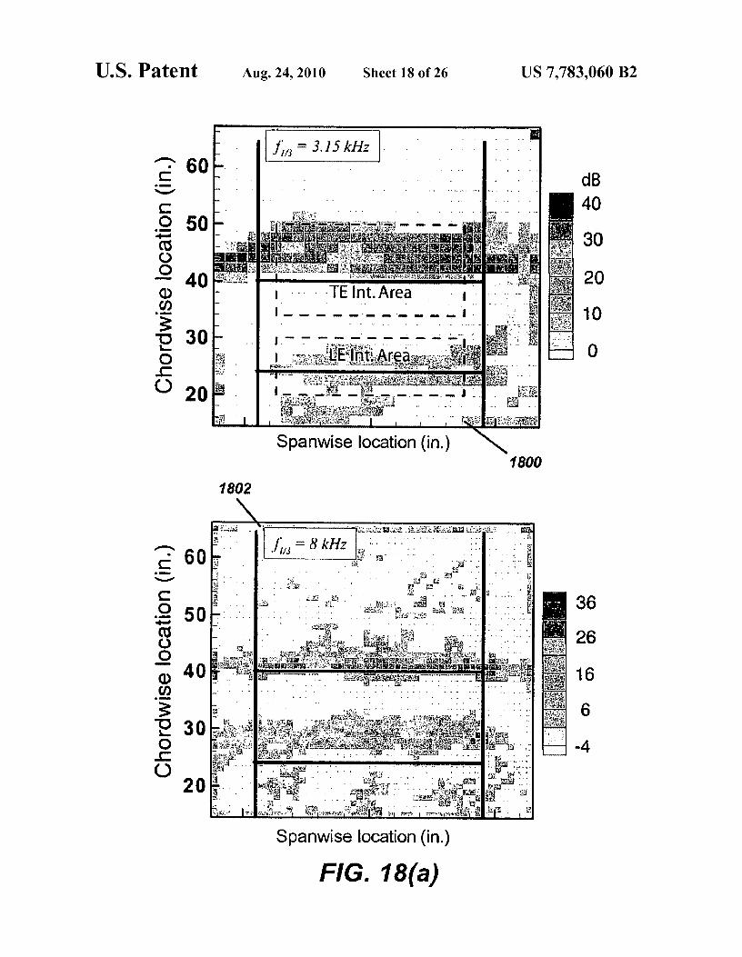
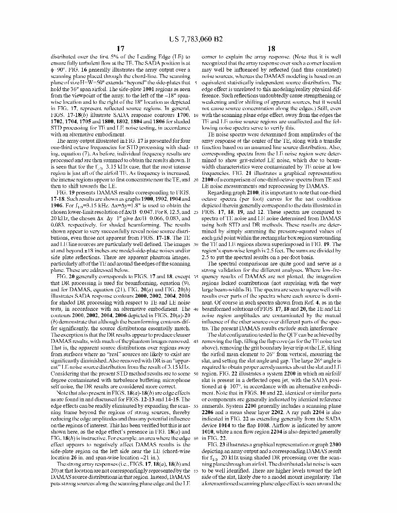
65 FIG. 17 and FIGS. 18(a)-18(b) illustrate SADA responsecontours for shaded STD processing for TE and LE noisetesting, in accordance with an alternative embodiment;

US 7,783,060 B25

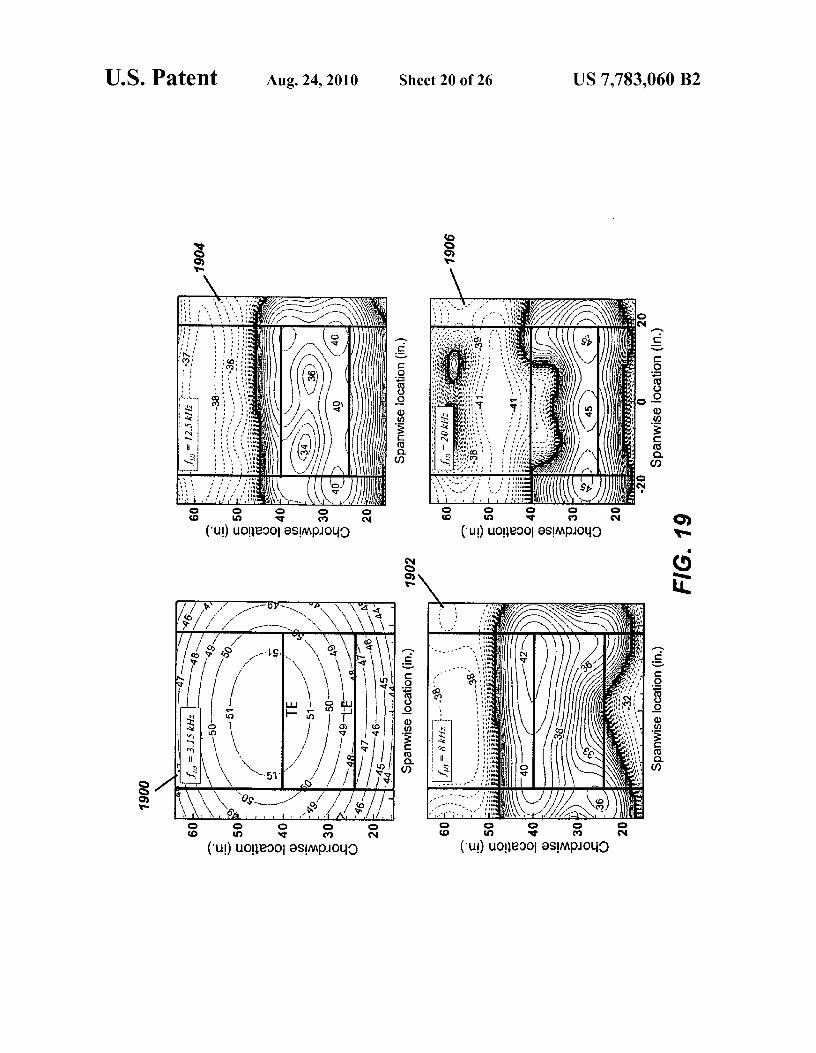
FIG. 19 illustrates DAMAS results corresponding to FIGS.17-18, in accordance with an alternative embodiment;

FIG. 20(a) and FIG. 20(b) illustrate SADA response con-tours for shaded DR processing with respect to TE and LEnoise tests, in accordance with an alternative embodiment;

FIG. 21 illustrates a graphical representation of a compari-son of one-third octave spectra from TE and LE noise mea-surements and reprocessing by DAMAS, in accordance withan alternative embodiment;

FIG. 22 illustrates shows an airfoil/slat in a deflected openjet, with a SADA positioned at ^-107;

FIG. 23 illustrates the array output and correspondingDAMAS result for f113=20 kHz using shaded DR processingover a scanning plane through an airfoil; and

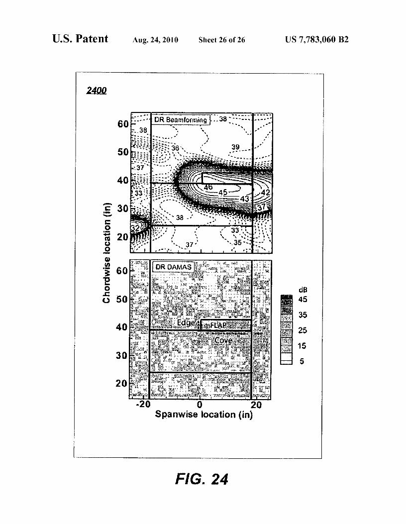
FIG. 24 illustrates beamforming contours and DAMASresults for shaded DR processing over a scanning planeplaced through an airfoil chord-line.

DETAILED DESCRIPTION

The particular values and configurations discussed in thesenon-limiting examples can be varied and are cited merely toillustrate at least one embodiment and are not intended tolimit the scope thereof. Additionally, acronyms, symbols andsubscripts utilized herein are summarized below.

Symbols and Acronymsam shear layer refraction amplitude correction for emA DAMAS matrix with A . componentsA,,,. reciprocal influence of beamforming characteristics

between grid pointsB array "beamwidth" of 3 dB down from beam peak maxi-mum

co speed of sound without mean flowCSM cross spectral matrixD nominal diameter of arrayDR diagonal removal of G in array processinge steering vector for array to focus locationem component of e for microphone mf frequencyAf frequency bandwidth resolution of spectraFFT Fast Fourier Transform

array elevation angleGmm . cross-spectrum between pm and pm.G matrix (CSM) of cross-spectrum elements Gmm.H height of chosen scanning planei iteration numberk counting number of CSM averages, also acoustic wave

number1 representative dimension of source geometry detailLADA Large Aperture Directional ArrayLE leading edgem microphone identity number in arraym' same as m, but independently variedm0 total number of microphones in arrayn grid point number on scanning plane(s)M wind tunnel test Mach numberN total number of grid points over scanning plane(s)pm pressure time records from microphone mPm Fourier Transform of pmQFF Quiet Flow FacilityQ„ idealized Pm for modeled source at n for quiescent acoustic

mediumr, distance rm for m being the center c microphonerm retarded coordinate distance to m, timc0R nominal distance of array from scanning planeSADA Small Aperture Directional Array

6STD standard or classical array processing

T complex transpose (superscript)TE trailing edgeT_ propagation time from grid point to microphone m

5 wm frequency dependent shading (or weighting) for mW shading matrix of wm termsW width of scanning planeAx widthwise spacing of grid pointsX matrix of X„ terms

io X„ "noise source" at grid point n with levels defined at array,Q1*Q1

Ay heightwise spacing of grid pointsY(e) output power response of the array at focus locationY matrix ofY„ terms

15 Y„ Y(e), when focused at grid point n

Subscriptsbkg backgrounddiag diagonal

20 m:n term associated with m, as it relates to grid position nmod modeled

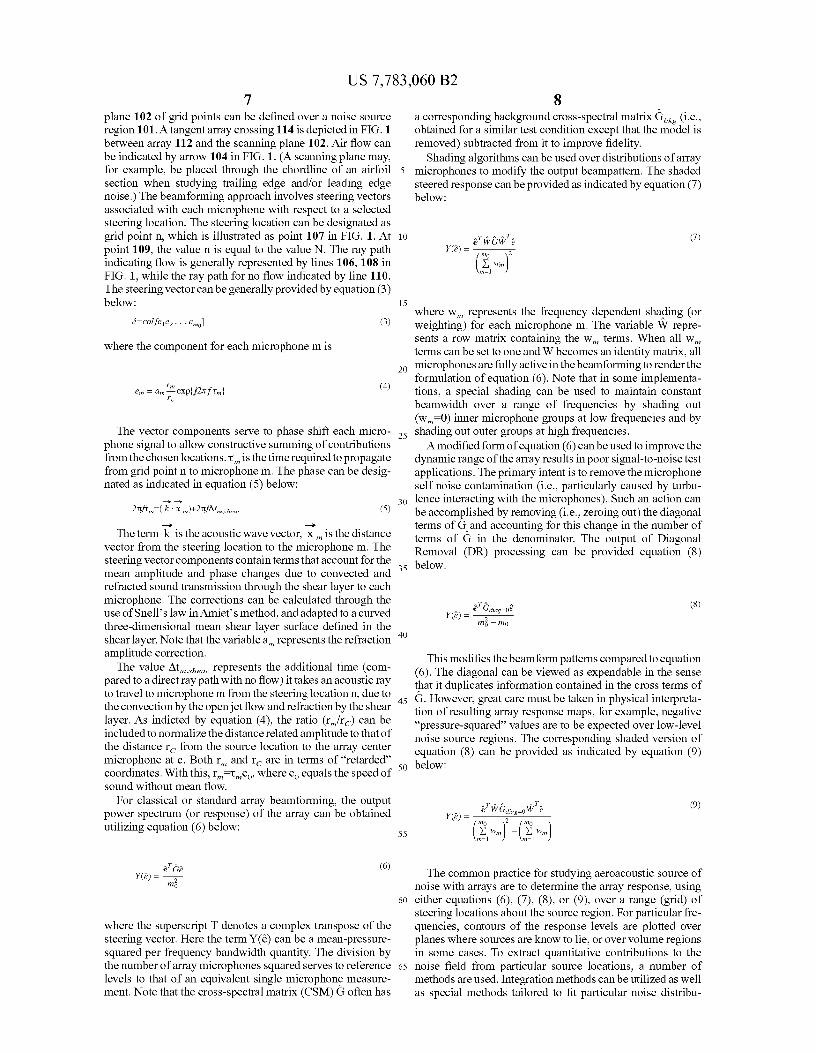
The first step in a DAMAS formulation or analysis is tobeamform over the source region, using what have becometraditional methods. Post processing of simultaneously

25 acquired data from the microphones of an array begins withcomputation of the cross-spectral matrix for each test casedata set. The computation of each element of the matrix isperformed using Fast Fourier Transforms (FFT) of the origi-nal data ensemble. The transform pairs P m (f,T) and P_.(f,T)are formed from pressure time records pm (t) and pm,(t),

30 defined at discrete sampling times that are At apart, of datablock lengths T from microphones m and m', respectively.The cross-spectrum matrix element can be provided as indi-cated in equation (1) below:

35

J^^^ rK111^ s s

G..'(Js

)— KW TY1, LPk (f, T)P.'k (f, T)]

40This one-sided cross-spectrum can be averaged over K

block averages. The total record length is T,,, KT. The termws represents a data-window (e.g., such as Hamming) weight-ing constant. Gmm ,(t) can be seen as a complex spectrum with

45 values at discrete frequencies f, which are Af apart. The band-width is Af^=1/T (Hz). The full matrix is, with m 0 being thetotal number of microphones in the array,

50Gil Gil ... Gi.0^^)

G22c-

L Gmo, Gmomo J

55

Note that the lower triangular elements are complex con-jugates of the upper triangular elements. The cross-spectralmatrix can be employed in conventional beamformingapproaches to electronically "steer" to chosen noise source

60 locations about an aeroacoustic test model.FIG. 1 illustrates an open jet configuration system 100

wherein a phased microphone array 112 is indicated as out offlow and a scanning plane thereof positioned over an aeroa-coustic source region, in accordance with one embodiment.

65 FIG. 1 generally depicts a particular test setup of a distri-bution of microphones of a phased array 112 located outsidethe flow field containing an aeroacoustic model. A scanning

a corresponding background cross-spectral matrix Gbkg (i.e.,obtained for a similar test condition except that the model isremoved) subtracted from it to improve fidelity.

Shading algorithms can be used over distributions of array5 microphones to modify the output beampattern. The shaded

steered response can be provided as indicated by equation (7)below:

10_T V CWT "e

Y(e) =z

^0

1 Wm

^T W (%,Y(e) =

20

^1 Wm

T (9j'g-0 V 2

04 wm=1

US 7,783,060 B27

plane 102 of grid points can be defined over a noise sourceregion 101. A tangent array crossing 114 is depicted in FIG.1between array 112 and the scanning plane 102. Air flow canbe indicated by arrow 104 in FIG. 1. (A scanning plane may,for example, be placed through the chordline of an airfoilsection when studying trailing edge and/or leading edgenoise.) The beamforming approach involves steering vectorsassociated with each microphone with respect to a selectedsteering location. The steering location can be designated asgrid point n, which is illustrated as point 107 in FIG. 1. Atpoint 109, the value n is equal to the value N. The ray pathindicating flow is generally represented by lines 106, 108 inFIG. 1, while the ray path for no flow indicated by line 110.The steering vector can be generally provided by equation (3)below:

e=col[e lez... em0] (3)

where the component for each microphone m is

(4)em = am rm—exp{j2)rfrm}rc

The vector components serve to phase shift each micro-phone signal to allow constructive summing of contributionsfrom the chosen locations. ti m is the time required to propagatefrom grid point n to microphone m. The phase can be desig-nated as indicated in equation (5) below:

2 'n. ftm (k - x m)+2jtfll .,shear (5)

The term k is the acoustic wave vector, x m is the distancevector from the steering location to the microphone m. Thesteering vector components contain terms that account for themean amplitude and phase changes due to convected and 35refracted sound transmission through the shear layer to eachmicrophone. The corrections can be calculated through theuse of Snell's law inAmiet's method, and adapted to a curvedthree-dimensional mean shear layer surface defined in theshear layer. Note that the variable a m represents the refraction 40amplitude correction.

The value Atm,shear represents the additional time (com-pared to a direct ray path with no flow) it takes an acoustic rayto travel to microphone m from the steering location n, due to 45the convection by the open j et flow and refraction by the shearlayer. As indicted by equation (4), the ratio (rm/rc) can beincluded to normalize the distance related amplitude to that ofthe distance rc from the source location to the array centermicrophone at c. Both rm and rc are in terms of "retarded"coordinates. With this, r m,tmco, where c o equals the speed of Sosound without mean flow.

For classical or standard array beamforming, the outputpower spectrum (or response) of the array can be obtainedutilizing equation (6) below:

55

^T Ce" (6)Y(P) = z

m0

60

where the superscript T denotes a complex transpose of thesteering vector. Here the term Y(e) can be a mean-pressure-squared per frequency bandwidth quantity. The division bythe number of array microphones squared serves to reference 65levels to that of an equivalent single microphone measure-ment. Note that the cross-spectral matrix (CS1V1) 6 often has

8

where wm represents the frequency dependent shading (orweighting) for each microphone m. The variable W repre-sents a row matrix containing the wm terms. When all wmterms can be set to one and W becomes an identity matrix, allmicrophones are fully active in the beamforming to render theformulation of equation (6). Note that in some implementa-tions, a special shading can be used to maintain constant

beamwidth over a range of frequencies by shading out

(w_=0) inner microphone groups at low frequencies and byshading out outer groups at high frequencies.

A modified form of equation (6) can be used to improve thedynamic range of the array results in poor signal-to-noise testapplications. The primary intent is to remove the microphoneself noise contamination (i.e., particularly caused by turbu-lence interacting with the microphones). Such an action canbe accomplished by removing (i.e., zeroing out) the diagonalterms of G and accounting for this change in the number ofterms of G in the denominator. The output of Diagonal

Removal (DR) processing can be provided equation (8)below:

^TCe;ag=oe (g)Y(e) =

zmo — mo

This modifies thebeamform patterns comparedto equation(6). The diagonal can be viewed as expendable in the sensethat it duplicates information contained in the cross terms ofG. However, great care must be taken in physical interpreta-tion of resulting array response maps, for example, negative"pressure-squared" values are to be expected over low-levelnoise source regions. The corresponding shaded version ofequation (8) can be provided as indicated by equation (9)below:

The common practice for studying aeroacoustic source ofnoise with arrays are to determine the array response, usingeither equations (6), (7), (8), or (9), over a range (grid) ofsteering locations about the source region. For particular fre-quencies, contours of the response levels are plotted overplanes where sources are know to lie, or over volume regionsin some cases. To extract quantitative contributions to thenoise field from particular source locations, a number ofmethods are used. Integration methods can be utilized as wellas special methods tailored to fit particular noise distribu-

15

20

25

30

US 7,783,060 B29

tions, depending upon design considerations. Still the meth-ods can be difficult to apply and care must be taken in inter-pretation. This is because the processing of equations (6)-(9)produces "source" maps which are as much a reflection of thearray beamforming pattern characteristics as is the source 5distribution being measured.

The purpose here is to pose the array problem such that thedesired quantities, the source strength distributions, areextracted cleanly from the beamforming array characteris-tics. First, the pressure transform P m of microphone m of toequation (1) is related to a modeled source located at positionn in the source field as indicated by equation (10) below:

Pm.,,=Q„em.,, i

(10)

10where the bracketed term is that of equation (12). This can beshown to equal

Y ,. p)=`4x, (16)

where the components of matrix A are

-T[ n, e"" (17)A mz

0

By equatingY„ m„ (e) withprocessedY(e) from measured data,we have

Here Q„ represents the pressure transform that P_ (or Pm)would be if flow convection and shear layer refraction did notaffect transmission of the noise to microphone m, and if mwere at a distance of r, from n rather than rm . The em .,,-i termrepresents simply those components that were postulated inequation (4) to affect the signal in the actual transmission torender the value P„,. The product of pressure-transform termsof equation (1) therefore becomes as indicated in equation(11) below:

P,n.,,Pm,.a = (Qn emin) * (Qnem':n) (11)

Q„Qn(emid *em':n

When this equation is substituted into equation (1), oneobtains the modeled microphone array cross-spectral matrixfor a single source located at n

(eii).eii (ei i ) * ez i ... (el l ) emo (12)

(ez i ) * e l l (ezi)*ezikm, = Xn

(em0) em0 n

where X„ is the mean square pressure per bandwidth at eachmicrophone m normalized in level for a microphone at r_—r,.It is now assumed that there are a number N of statisticallyindependent sources, each at different n positions. Oneobtains for the total modeled cross-spectral matrix

Cmod = O'nmod(13)

Employing this in equation (6),

Ynmod (e)

= ^eT( z

de n

(14)

m0

en Y Xn, q n^ en (15)en

Ynmod (e) =

zq

z en X”

m0 — m0

15 lik k

(18)

Equation (18), for X, also applies for the cases of shadedstandard, DR, and shaded DR beamforming, with compo-nents A_. o0, becoming

20

eT T (19)W qn,W e

Ann = 0 z

t Wm)

25

e(20)

Ann = n(q n^)d;og=oen

,M2m0 — mo

and

30 T (21)Ten W (q ) og— W eenAnn _ n di 0

1

Wm\ 2 —

4rZ _)2

mo

35

respectively. For standard beamforming (shaded or not) thediagonal terms for A are equal to one. For Diagonal Removalbeamforming (shaded or not), the diagonal terms for A arealso equal to one, but the off-diagonal components differ and

40 attain negative values when n and n' represent sufficientlydistant points from one another, depending on frequency.

Equation (18) represents a system of linear equations relat-ing a spatial field of point locations, with beamformed array-output responses Y,,, to equivalent source distributions X„ at

45 the same point locations. The same is true of equation (18)when Y„ is the result of shaded and/or DR processing of thesame acoustic field. X„ is the same in both cases. (One is notrestricted to these particular beamforming processing as longas A is ' defined.) Equation (18) with the appro-

50 priate A defines the DAMAS inverse problem. It is unique inthat it or an equivalent equation must be the one utilized inorder to disassociate the array itself from the sources beingstudied. Of course, the inverse problem must be solved inorder to render X. Equation (18) can therefore be thought of

55 as constituting a DAMAS inverse formulation. Equations(22) to (24), on the other hand, which are describe in greaterdetail below, make solutions possible and thus function as aunique iterative method.

Equation (18) represents a system of linear equations.

60 Matrix A is square (of size NxN) and if it were nonsingular(well-conditioned), the solution would simply be X=A` '.However, it has been found for the present acoustic problemsof interest that only for overly restricted resolution (distancebetween n grid points) or noise region size (spatial expanse of

65 the N grid points) would A be nonsingular. Using a SingularValue Decomposition (SVD) methodology for determiningthe condition of A, it is found that for resolutions and region

US 7,783,060 B2

A„ iX,+A y +... +A y +... +A y -P (22) 202"2 rf'n nZW'N

11sizes of common interest in the noise source mapping prob-lem in aeroacoustic testing that the rank of A can be quitelow often on the order of 0.25 and below.

Rank here can be defined as the number of linearly inde-pendent equations compared to the number of equations ofequation (18), which is N=number of grid points. This meansthat generally very large numbers of"solutions" are possible.Equation (18) and the knowledge of the difficulty with equa-tion rank were determined early in the present study. TheSVD solution approach with and without a regularizationmethodology special iterative solving methods such as Con-jugate Gradient methods and others did not produce satisfac-tory results. Good results were ultimately obtained by a verysimple tailored iterative method where a physically-neces-sary positivity constraint (making the problem deterministic)on the X components could be applied smoothly in the itera-tion. This is described below.

A single linear equation component of equation (18) is

With A,,,,=1, this is rearranged to give

- 1 N (23)

X„ = n - A, X„ + A, X„

n —

This equation is used in an iteration methodology to obtainthe source distribution X„ for all nbetween 1 and N as per thefollowing equation.

X 11') = Y - ^0 + N A,,,

^)^

(24)

- NXii) = n - A_, Xn) + A,,,,, X (,% i)

n-

N-^XN) = YN - AN,, Xni + 0

For the first iteration (i=1), the initial values X„ can betaken as zero orY„ (the choice appears to cause little differ-ence in convergence rates). It is seen that in the successivedetermination of X,,, for increasing n, the values are continu-ously fed into the succeeding X„ calculations. After each X„determination, if it is negative, its value is set to zero. Eachiteration (i) can be completed by like calculations, butreversed, moving from n=N back to n=1. The next iteration(41) starts again at n=1. Equation (24) is the DAMAS inverseproblem iterative solution.

FIG. 2 illustrates a system 200 including key geometricparameters of a phased microphone array 112 and a sourcescanning plane 202, in accordance with an embodiment. Notethat the source scanning plane 202 depicted in FIG. 2 isgenerally analogous to the source scanning plane 102depicted in FIG. 1. In general, FIG. 2 provides identifiedimportant parameters in defining the solution requirementsfor DAMAS for a scanning plane 102. The array has a spatialextent defined by the "diameter" D. It is at a nominal distanceR from a scanning plane containing N grid points, whichrepresent beamforming focal points, as well as the n locationsof all the acoustic sources X„ that influence the beamformed

12results Y,,. Note that in FIG. 2, circles 203 generally representdB level contours over the grid(s) of the source scanningplane 202.

For a particular frequency, the array's beamformed output5 is shown projected on the plane as contour lines of constant

outputY, in terms of dB. The scanning plane has a height of Hand a width of W. The grid points are spaced Ax and Ay apart.Although not illustrated in FIG. 2, there are defined noisesource sub-regions of size 1 within the scanning plane (subsets

10 of X„ ), where details are desired. This relates to source reso-lution requirements and is considered below. For the scanningplane, the total number of grid points,

A [(W/Ax)+i][(xioy)+i] (25)

15 The array beamwidth B is defined as the "diameter" of the3 dB-down output of the array compared to that at the beam-formed maximum response. For standard beamforming ofequation (6),

R.^oonetk(R/fDl

(26)

For the SADA (Small Aperture Directional Array with a outerdiameter of D-0.65 feet) in a traditional QFF configuration'with R=5 feet, the beamwidth is B-(104/f) in feet for fre-quency f in Hertz. When using shading of equation (7), B is

25 kept at about 1 ft. for 10 kHz^f;^40 kHz.In the applications of this report, some engineering choices

are made with regard to what should represent meaningfulsolution requirements for DAMAS source definition calcula-

30 tions. Because the rank of matrix A of equation (18) equalsone when using the iterative solution equation (24), there is nodefinitive limitation on the spacing or number of grid pointsor iterations to be used. The parameter ratios Ax/B (and Ay/B)and W/B (and H/B) appear to be most important for estab-

35 lishing resolution and spatial extent requirements of the scan-ning plane.

The resolution Ax/B must be small or fine enough such thatindividual grid points along with other grid points represent areasonable physical distribution of sources. However, too fine

40 of a distribution would require substantial solution iterativetimes and then only give more detail than is realisticallyfeasible, or believable, from a beampattern which is toobroad. On the other hand, too coarse of a distribution wouldrender solutions of X which would reveal less detail than

45 needed, and also which may be aliased (in analogy with FFTsignal processing), with resulting false images.

The spatial extent ratio W/B (and H/B) must be largeenough to allow discrimination of mutual influence betweenthe grid points. Because the total variation of level over the

50 distance B is only 3 dB, it appears reasonable to require that1 <W/B (and H/B). One could extend W/B (and H/B) substan-tially beyond one such as to five or more. In the followingsimulations, resolution issues are examined for both a simpleand a complicated noise source distribution. Two distribu-

55 tions types are considered because, as seen below withrespect to 1/B, source complexity affects source definitionconvergence. The simulations also serve as an introduction tothe basic use of DAMAS.

Regarding execution efficiency of the DAMAS technique,60 it is noted that the per-iteration execution time of the meth-

odology depends solely on the total number of grid pointsemployed in the analysis and not on frequency-dependentparameters. In general, the iteration time can be expressed bytime=C(2N)2i, where C is a hardware-dependent constant. A

65 representative execution time is 0.38 seconds/iteration run-ning a 2601-point grid on a 2.8-GHz, Linux-based Pentium 4machine using Intel Fortran to compile the code. For this

US 7,783,060 B2

13

14study, a Beowulf cluster consisting of nine 2.8 GHz Pentium4 machines was used to generate the figures shown subse-quently. Note that in FIG. 2, the value B generally representsthe diameter of three circles.

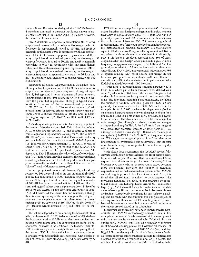
FIG. 3 illustrates a graphical representation 300 of arrayoutput based on standard processing methodologies, whereinfrequency is approximately equal to 10 kHz and Ax/B isgenerally equivalent to 0.083 in accordance with one embodi-ment. FIG. 4 illustrates a graphical representation 400 ofarray output based on standard processing methodologies,wherein frequency is equal to 20 kHz and Ax/B is generallyequivalent to 0.167 in accordance with one embodiment.Likewise, FIG. 5 illustrates a graphical representation 500 ofarray output based on standard processing methodologies,wherein frequency is approximately equal to 30 kHz andAx/B is generally equivalent to 0.25 in accordance with oneembodiment;

In a traditional contour type presentation, the top left frameof the graphical representation of FIG. 3 illustrates an arrayoutput based on standard processing methodology of equa-tion (6), being plotted in terms of constant dB contours over ascanning plane. In this simulation, the SADA is placed 5 feetfrom the plane that is positioned through a typical modellocation. In terms of the aforementioned parameters,H=W=50" and Ax=Ay=1". The resultant number of gridpoints is 2601 (underlying grid points are not shown in top leftframe). With a chosen frequency of 10 kHz and the beam-forming of equation (6), B-12", so H/B=W/B=4.17 andAx/B=0.083.

A single synthetic point source is placed at a grid point inthe center of the plane, at n=1301. This is done by definingX 1301 to give 100 dB=10LogX 1301 and all other X values tozero in equation (18), and then solving for Y. The values ofdB=10LogY„ are then contour plotted. This, as withreal arraytest data, is the starting point for the use of DAMAS. Equation(18) is solved for X using equation (17) for A,,,,,, by way ofequation (24), using X„ Y„ at the start of the iteration. Thebottom left frame of the graphical representation 300depicted in FIG. 3 illustrates the values of X„ after one itera-tion (i=1). Rather than showing contours, the presentation isone of X„ values in terms of dB at the grid points. Each gridpoint is actually located at the bottom left corner of the"blocks", each of dimension Ax—Ay-1".

In the top right and bottom right frames of graphical rep-resentation 300 the results after the one thousandth (i=1000)and the five thousandth (i=5000) iteration, respectively, areshown. At the highest iteration value, the original input valueof 100 dB has been recovered within 0.1 dB and that thesurrounding grid values over the plane are down in level byabout 40 dB, except for the adjoining grid points at about15-20 dB down. At the lesser iteration numbers, althoughthere is some spreading of the source region, the integrated(obtained by simple summing of values over the spreadregion) levels are very close to 100 dB. One obtains 99.06 dBfor 100 iteration (not shown in FIG. 3) and 100.03 dB for 1000iterations.

The solution dependence on reducing the beamwidth B bya factor of two (Ax/B-0.167) is demonstrated in FIG. 4 wherethe frequency used is 20 kHz using the same standard pro-cessing over the same grid. The contour pattern is similar, butcontracted, as shown in the left frame. The DAMAS result for1000 iterations is given in the right frame. Comparing this tothe results of FIG. 3, it is seen that here a more exact solutionis attained with substantially less iterations. One obtains atpeak of 99.97 dB, with all adjoining grid points lower by 27dB.

FIG. 6 illustrates a graphical representation 600 of an arrayoutput based on standard processing methodologies, whereinfrequency is approximately equal to 10 kHz and Ax/B isgenerally equivalent to 0.083 in accordance with an alterna-

5 tive embodiment. Likewise, FIG. 7 illustrates a graphicalrepresentation 700 of array outputbased on standard process-ing methodologies, wherein frequency is approximatelyequal to 20 kHz and Ax/B is generally equivalent to 0.167 inaccordance with an alternative embodiment. Additionally,

io FIG. 8 illustrates a graphical representation 800 of arrayoutput based on standard processing methodologies, whereinfrequency is approximately equal to 30 kHz and Ax/B isgenerally equivalent to 0.25 in accordance with an alternativeembodiment. FIG. 9 illustrates a graphical representation 900

15 of spatial aliasing with point source and image shiftedbetween grid points in accordance with an alternativeembodiment. FIG. 9 demonstrates the implementation of aDAMAS methodology with 1000 iterations.

The results of a more demanding simulation are depicted in20 FIGS. 6-8, where particular n locations were defined with

same X„ values (for 100 dB) and others zero. This gives a testof the solution procedure for a group of line source distribu-tions. The important scanning plane parameters, includingthe number of solution iterations, given for FIGS. 6-8 are

25 generally the same as above for FIGS. 2-5. In FIG. 6, forexample, for Ax/B-0.083, the beamforming contour plot hasan elongated appearance as one would expect to obtain for aline source. After using 5000 iterations, however, one beginsto see structure other than a line source. Still, the image has

3o not converged (i.e., although not shown, it starts to convergesat higher iterations). In FIG. 7, for Ax/B-0.167, an image ofvery prominent character emerges at 1000 iterations (i.e.,although not shown, even at only 100 iterations the image isrecognizable). In FIG. 8, for Ax/B=0.25, all images are appar-

35 ent. With regard to integrated power, it is found that whenintegrating (e.g., by summing grid point values), that the totalnoise from the image converges to the correct value rapidlywith iterations.

Such simulations demonstrate that DAMAS successfully40 extracts detail noise source information from phased array

beamformed outputs. It is seen that finer Ax/B resolutionsrequire more iterations to get the same "accuracy." Thisbecomes even more valid as the noise source region becomesmore complicated. However, the number of iterations

45 required should not be the major driving issue as the DAMASmethodology is proven to be efficient and robust. Also, it isfound that all solutions, examined to date, improve withincreasing iterations (i.e., using double precision computa-tions). Caution is noted for potential error if Ax/B is made too

50 large (e.g., Ax/B above 0.2 may be borderline) in real datacases where significant sources may be in-between chosengrid points. As previously mentioned for any such error, anal-ogy can be made with the common data analysis subject ofaliasing errors with respect to FFT sampling rates. No prob-

55 lems of this nature are possible in these simulations becausethe sources are collocated at the grid points.

Experimental applications have been implemented to dem-onstrate the DAMAS methodology described herein. Forexample, experimental data from several airframe component

6o noise studies can be re-examined with DAMAS. In suchapplications, DAMAS is not used with necessarily optimumresolution and scanning plane size. However, all cases fall ator near an acceptable range of 0.05-Ax/B (i.e., and Ay/B)- 0.2. For consistency with the simulations, (except for the

65 calibrator case) the same scanning plane and resolution sizesare used with the same resultant number of grid points. Thenumber of iterations used for all is 1000. In contrast with the

US 7,783,060 B215

16simulations, the experimental results are presented in terms of

Ax/13-0.046 (which is close to the recommended lower limit

one-third octave values, for the array using several different of 0.05). The number of grid points is 441 and the number ofarray beamforming methodologies, in order to compare to the

iterations used is 1000 for each frequency.

results of the previous studies. Note that a characteristic of the DAMAS solution is theFIGS. 10 and 11 respectively illustrate configurations 1000 5 non-negligible amplitudes distributed at grid points around

and 1100 of a test set up for flap edge noise test and calibra- the border of the scanning planes in FIG. 13. This is a scan-tion. In configuration 1000 of FIG. 10, for example, the noise ningplane "edge" effect that is foundto occur only for experi-path from the flap edge to a SADA device 1014 is illustrated

mental data, where noise in the scanning plane is influenced

as represented by ray path 1006. A mean shear layer 1004 is to some degree by sources outside (or extraneous to) thedepicted in FIG. 10 in association with a shear layer 1002. io plane. DAMAS constructs noise distribution solutions on theArrow 1010 depicted in FIG. 10 represents airflow from a scanning plane grid points totally based on whatever is mea-nozzle 1012. A flap model 1008 is also depicted in FIG. 10. sured by beamforming on those grid points. The edge effectThe nozzle 1012 is located adjacent to and/or integrated with

was examined by expanding the scanning plane to eliminate

a side plate 1001. any edge problem in the region of interest. A result almostIn configuration 1000 of FIG. 11, on the other hand, the 15 identical to FIG. 12 was found over regions other than at the

open end of a calibrator source is depicted positioned next to edge. Thus the edge effect has negligible impact on thesethe edge of flap 1008. Note that in FIGS. 10-11, identical or results. This subject is dealt with subsequently for other appli-similar parts or elements are generally indicated by identical

cations.

reference numerals. Thus, FIGS. 10-11 should be interpreted

A small rectangular integration region, illustrated bytogether. A sketch of the flap edge noise experimental setup is 20 dashed lines in FIG. 12, can be used to calculate an integratedtherefore depicted in configuration 1000 of FIG. 10, wherein value of 62.8 dB. Correspondingly, for the present DAMASan airfoil main element is located at a 16° angle-of-attack to result, one simply adds the pressure-squared values of thethe vertical plane. The SADA device 1014 is shown posi- grid points within the source region. One obtains a value oftioned out of or away from the flow represented by arrow

62.9 dB. FIG. 13 illustrates the SADA response contour for

1010 in FIG. 10. For configuration 1000 depicted in FIG. 10, 25 the tunnel flow at M=0.17. Here, the convective and shearthe calibration test can be performed using a noise source, layer refraction terms are important in the steering vectorcomprised of an open end of a one-inch diameter tube, placed

definition. The integrated value from Ref. 1 is 58.1 dB,

next to the flap edge, as depicted in configuration 1100 of

whereas the DAMAS value is 57.3 dB. It is seen by compar-FIG. 11. Note that in the configuration illustrated in FIG. 11, ing the somewhat smeared image of FIGS. 12-13 that thea calibration source 1102 is shown proximate to the flap 1008. 3o affect of the tunnel flow and the resultant turbulent shear layer

FIG. 12 illustrates a graphical representation 1200 of cali- is to spread the apparent noise region. The DAMAS result inbrator source test data wherein M-0 with an integrated level

FIG. 13 is of particular interest because, to the knowledge of

of 62.8 dB and a DAMAS of 62.9 dB, in accordance with an the authors, it may be the first direct measure of spatial dis-alternative embodiment. Similarly, FIG. 13 illustrates a persion of noise due to turbulence scatter.graphical representation 1300 of calibrator source test data 35 For the same test cases as FIGS. 12-13. 7, FIGS. 14-15wherein M=0.17, with an integrated level of 58.1 dB and a

illustrate results when diagonal removal (DR), equation (9), is

DAMAS of 57.3 dB, in accordance with an alternative employed in the beamforming. Correspondingly, DAMAS isembodiment. FIG. 14 illustrates a graphical representation applied using equation (21) for A,,,,.. It is seen that although1400 of a calibrator source test, wherein M-0 with an inte- the DR processing modifies the distributions, the X sourcegrated level of 62.2 dB and a DAMAS of 61.6 dB, in accor- 4o distributions and values are calculated to be almost identicaldance with an alternative embodiment. FIG. 15 illustrates a to those of FIGS. 12-13. DR processing has the advantage ofgraphical representation 1500 of a calibrator source test, removing the auto-spectra (and possible microphone noisewherein M-0.17 with an integrated level of 57.9 dB and a contamination) from the processing, while still maintainingDAMAS of 56.9, in accordance with an alternative embodi- full rank for the solution equations.ment; 45 Although it is beyond the scope of this paperto evaluate the

FIGS. 12 and 13 respectively illustrate DAMAS results use of DAMAS for different array designs than the SADA, afrom an experimental implementation thereof. For the cali- limited application using Large Aperture Directional Arraybrator source operating with no tunnel flow M-0, FIG. 12

(LADA) data produced good comparisons for a case corre-

shows SADA response contours for standard (STD) process- sponding to a frame of FIG. 12. The LADA has an outering with shading, equation (7), over a scanning plane posi- 5o diameter of D=2.83 feet, which is 4.35 times the size oftioned through the airfoil chord-line. This is a one-third

SADA (i.e., 17.4 times the active diameter of the SADA at 40

octave presentation for l OLogY for f113=40 kHz. The result

kHz for shaded processing). For a similar calibration test towas obtained by performing and summing 546 single-fre- that of FIG. 12 but for array processing without shading, thequency beamforming maps (each with frequency resolution

integrated LADA value is 60.3 dB, and the corresponding

bandwidth of Af^=17.44 Hz). Note that with this array-shad- 55 DAMAS summed value is 61.4 dB.ing, only the inner SADA diameter of 1.95 inches is active. A test configuration can be implemented where an airfoil,For this no-flow case, the convective and shear layer refrac- with a 16" chord and 36" span, is positioned at a -1.2° angle-tion terms are absent in the steering vector definition, equa- of-attack to the vertical flow is depicted in FIG. 16. Note thattions (4) and (5). in FIGS. 10-11 and 16, identical or similar parts or elements

The right frame of FIG. 12 illustrates the result for the 6o are generally indicated by identical reference numerals. Asrendered source X distribution when DAMAS is applied, indicated in FIG. 16, a mean shear layer 1602 and 1604 aresolving equation (18), and using equation (19), by way of

illustrated with respect to side-plate 1001 and flap 1008. Flow

equation (24). The scanning plane used is H=W=12". Con- is generally indicated by arrow 1010, while a ray path 1606 tosistent with the contour presentation, the DAMAS result is a the SADA device 1014 is also depicted.one third octave presentation obtained by separately solving 65 The flap 1008 can be removed and a cove thereof filled infor the 546 separate bands and then summing. With B=12"

such a manner as to produce a span-wise uniform sharp Trail-

and a chosen Ax=Ay=0.55", one has a resolution of

ing Edge (TE) of 0.005". A grit of size #90 is generally

US 7,783,060 B217

18distributed over the first 5% of the Leading Edge (LE) to corner to explain the array response. (Note that it is wellensure fully turbulent flow at the TE. The SADA position is at recognized that the array response over such a corner location^-90°. FIG. 16 generally illustrates the array output over a may well be influenced by reflected (and thus correlated)scanning plane placed through the chord-line. The scanning noise sources, whereas the DAMAS modeling is based on anplane of size H=W=50" extends "beyond" the side-plates that 5 equivalent statistically independent source distribution. Thehold the 36" span airfoil. The side-plate 1001 regions as seen edge effect is unrelated to this modeling/reality physical dif-from the viewpoint of the array, to the left of the —18" span- ference. Such reflections undoubtedly cause strengthening orwise location and to the right of the 18" location as depicted

weakening and/or shifting of apparent sources, but it would

in FIG. 17, represent reflected source regions. In general, not cause source concentration along the edges.) Still, evenFIGS. 17-18(b) illustrate SADA response contours 1700, io with the scanning plane edge effect, away from the edges the1702, 1704, 1705 and 1800, 1802, 1804 and 1806 for shaded

TE and LE noise source regions are unaffected and the fol-

STD processing for TE and LE noise testing, in accordance

lowing noise spectra serve to verify this.with an alternative embodiment. TE noise spectra were determined from amplitudes of the

The array output illustrated in FIG. 17 is presented for four array response at the center of the TE, along with a transferone-third octave frequencies for STD processing with shad- 15 function based on an assumed line source distribution. Also,ing, equation (7). As before, individual frequency results are corresponding spectra from the LE noise region were deter-processed and are then summed to obtain the results shown. It mined to show grit-related LE noise, which due to beam-is seen that for the 1`

113=3.15 kHz case, that the most intense width characteristics were contaminated by TE noise at low

region is just aft of the airfoil TE. As frequency is increased, frequencies. FIG. 21 illustrates a graphical representationthe intense regions appear to first concentrate near the TE, and 20 2100 of a comparison of one-third octave spectra from TE andthen to shift towards the LE. LE noise measurements and reprocessing by DAMAS.

FIG. 19 presents DAMAS results corresponding to FIGS. Regarding graph 2100, it is important to note that one-third17-18. Suchresults are shown as graphs 1900, 1902, 1904 and

octave spectra (per foot) curves for the test conditions

1906. For 1` 113=3.15 kHz, Ax=Ay=1.8" is used to obtain the

depicted therein generally correspond to the data illustrated in

chosen lower-limit resolution of Ax/B-0.047. For 8, 12.5, and 25 FIGS. 17, 18, 19, and 12. These spectra are compared to20 kHz, the chosen Ax—Ay-1" give Ax/B=0.066, 0.083, and

spectra of TE noise and LE noise determined from DAMAS

0.083, respectively, for shaded beamforming. The results using both STD and DR methods. These results are deter-shown appear to very successfully reveal noise source distri- mined by simply summing the pressure-squared values ofbutions, even those not apparent from FIGS. 17-18. The TE

each grid point within the rectangular box region surrounding

and LE line sources are particularly well defined. The images 30 the TE and LE regions shown superimposed in FIG. 19. Theat and beyond ±18 inches are model-side-plate noises and/or region's span-wise length is 2.5 feet. The sums are divided byside plate reflections. There are apparent phantom images, 2.5 to put the spectral results on a per-foot basis.particularly aft of the TE and around the edges of the scanning

The spectral comparisons are quite good and serve as a

plane. These are addressed below. strong validation for the different analyses. Where low-fre-FIG. 20 generally corresponds to FIGS. 17 and 18, except 35 quency results of DAMAS are not plotted, the integration

that DR processing is used for beamforming, equation (9), regions lacked contributions (not surprising with the veryand for DAMAS, equation (21). FIG. 20(a) and FIG. 20(b)

large beam-widths B). The spectra are seen to agree well with

illustrates SADA response contours 2000, 2002, 2004, 2006 results over parts of the spectra where each source is domi-for shaded DR processing with respect to TE and LE noise nant. Of course in such spectra shown from Ref. 4, as in thetests, in accordance with an alternative embodiment. The 4o beamformed solutions of FIGS. 17,18 and 20, the TE and LEcontours 2000, 2002, 2004, 2006 depicted in FIGS. 20(a)-20 noise region amplitudes are contaminated by the mutual(b) demonstrate that although the beamforming contours dif- influence of the other source over different parts of the spec-fer significantly, the source distributions essentially match. tra. The present DAMAS results exclude such interference.The exception is that the DR results appear to produce cleaner

The slat configuration tested in the QFF can be achieved by

DAMAS results, with much of the phantom images removed. 45 removing the flap, filling the flap cove (as for the TE noise testThat is, the apparent source distributions over regions away above), removing the grit boundary layer trip at the LE, tiltingfrom surfaces where no "real" sources are likely to exist are the airfoil main element to 26° from vertical, mounting thesignificantly diminished. Also removed with DR is an "appar- slat, and setting the slat angle and gap. The large 26° angle isent" LE noise source distribution from the result of 3.15 kHz. required to obtain proper aerodynamics about the slat and LEConsidering that the present STD method results are to some 5o region. FIG. 22 illustrates a system 2200 in which an airfoil/degree contaminated with turbulence buffeting microphone slat is present in a deflected open jet, with the SADA posi-self noise, the DR results are considered more correct. tioned at ^-107, in accordance with an alternative embodi-

Note that also present in FIGS. 18(a)-18(b) are edge effects ment. Note that in FIGS. 10 and 22, identical or similar partsas are found in and discussed for FIGS. 12-13 and 14-15. The or components are generally indicated by identical referenceedge effects can be readily eliminated by expanding the scan- 55 numerals. System 2200 generally includes a scanning planening frame beyond the regions of strong sources, thereby

2206 and a mean shear layer 2202. A ray path 2204 is also

reducing the edge amplitudes and thus any potential influence

indicated in FIG. 22 as extending generally from the SADAon the regions of interest. This has been verified but this is not

device 1014 to the flap 1008. Airflow is indicated by arrow

shown here, as the edge effect's presence in FIG. 18(a) and

1010, white anon flow region 2204 is also depicted generallyFIG. 18(b) is instructive. For example, an area where the edge 60 in FIG. 22.effect appears to negatively affect DAMAS results is the

FIG. 23 illustrates a graphical representation or graph 2300

side-plate region on the left side near the LE (chord-wise

depicting an array output and a corresponding DAMAS resultlocation 26 in. and span-wise location —21 in.). for 1`

113=20 kHz using shaded DR processing over the scan-

The strong array responses (i.e., FIGS. 17,18(a),18(b) and

ning plane through an airfoil. The distributed slat noise is seen20) at that location are not correspondingly represented by the 65 to be well identified. There are higher levels toward the leftDAMAS source distributions in that region. Instead, DAMAS

side of the slat, likely due to a model mount irregularity. The

puts strong sources along the scanning plane edge and the LE

aforementioned scanning plane edge effect is seen around the

US 7,783,060 B2

19

20edge of the DAMAS presentation, and it likely has a mildimpact on the source definition details at this left side. Awayfrom the edge, the slat noise is generally uniform. The ampli-tude of the slat noise is determined by summing across thespan within the integration box shown. For this one-thirdoctave band, the DAMAS level of 57.9 dB (per foot) com-pares with 59.1 dB, which has been used as an approximateprocedure involving the array output at the slat center and aderived transfer function.

The flap edge noise test configuration is illustrated in FIG.12 for the SADA. The flat edge flap test condition of 29° flapangle and M-0.11 is reexamined for a one-third octave fre-quency band of f113=20 kHz. FIG. 24 illustrates a graphicalrepresentation 2400 of beamforming contours and DAMASresults for shaded DR processing over the scanning planeplaced through the airfoil chord-line. The DAMAS resultsappear to successfully isolate the flap edge noise from sub-stantial flap cove noise. By using a similar rectangular inte-gration region, shown in FIGS. 12-13 and 14-15, one finds alevel of 44.6 dB for the flap edge noise. This compares to 47.5dB for a spectrum level determined for this flap edge noisecase. In that spectrum, this frequency corresponds to a local-ized spectral hump. These present results show that the covenoise contributed to the higher level measured. DAMAS isseen to allow one to readily separate and quantify these coverand flap edge contributions, where previously this was notpossible.

The DAMAS technique described herein represents a radi-cal step in array processing capabilities. It can replace tradi-tional presentations of array results and make the array amuch more powerful measurement tool than is presently thecase. The DAMAS equation Ax=Y is a unique equation thatrelates a classical beamformed array result Y with the sourcedistribution k The sources are taken as distributions of sta-tistically independent noise radiators, as does traditionalarray processing/integration analysis. DAMAS does not addany additional assumption to the analysis. It merely extractsthe array characteristics from the source definition presenta-tion. The iterative solution for X is found to be robust andaccurate. Numerical application examples show that theactual rate and accuracy at which solutions converge dependon chosen spatial resolution and evaluation region sizes com-pared to the array beam width. Experimental archival datafrom a variety of prior studies are used to validate DAMASquantitatively. The same algorithm is found to be equallyadept with flap edge/cove, trailing edge, leading edge, slat,and calibration noise sources

The foregoing methodology thus is generally directedtoward overcoming the current processing of acoustic arraydata, which is burdened with considerable uncertainty. Such amethodology can serve to demystify array results, reducemisinterpretation, and accurately quantify position andstrength of acoustic sources. As indicated earlier, traditionalarray results represent noise sources that are convolved witharray beam form response functions, which depend on arraygeometry, size (with respect to source position and distribu-tions), and frequency. The Deconvolution Approach for theMapping of Acoustic Sources (DAMAS) methodologydescribed above therefore removes beamforming character-istics from output presentations. A unique linear system ofequations accounts for reciprocal influence at different loca-tions over the array survey region. It makes no assumptionbeyond the traditional processing assumption of statisticallyindependent noise sources. The full rank equations are solvedwith a new robust iterative method.

DAMAS can be quantitatively validated using archivaldata from a variety of prior high-lift airframe component

noise studies, including flap edge/cove, trailing edge, andleading edge, slat, and calibration sources. Presentations areexplicit and straightforward, as the noise radiated from aregion of interest is determined by simply summing the mean-

5 squared values over that region. It is believed DAMAS canfully replace existing array processing and presentationsmethodology in most applications. Such a methodologyappears to dramatically increase the value of arrays to thefield of experimental acoustics.

10 It is important to note that the methodology describedabove with respect to FIGS. 1-23 and equations (1) to (26),which is referred to generally by the DAMAS acronym, canbe implemented in the context of a module(s). In the com-puter programming arts, a module (e.g., a software module)

15 can be implemented as a collection of routines and data struc-tures that perform particular tasks or implement a particularabstract data type. Modules generally can be composed oftwo parts. First, a software module may list the constants, datatypes, variable, routines and the like that that can be accessed

20 by other modules or routines. Second, a software module canbe configured as an implementation, which can be private(i.e., accessible perhaps only to the module), and that containsthe source code that actually implements the routines or sub-routines upon which the module is based.

25 Thus, for example, the term "module," as utilized hereingenerally refers to software modules or implementationsthereof. The world module can also refer to instruction mediaresiding in a computer memory, wherein such instructionmedia are retrievable from the computer memory and pro-

mo cessed, for example, via a microprocessor. Such modules canbe utilized separately or together to form a program productthat can be implemented through signal-bearing media,including transmission media and recordable media.

It will be appreciated that variations of the above-disclosed35 and other features and functions, or alternatives thereof, may

be desirably combined into many other different systems orapplications. Also that various presently unforeseen or unan-ticipated alternatives, modifications, variations or improve-ments therein may be subsequently made by those skilled in

40 the art which are also intended to be encompassed by thefollowing claims.

What is claimed is:45 1. A method for mapping acoustic sources determined from

a phased microphone array, comprising a plurality of micro-phones arranged in an optimized grid pattern including aplurality of grid locations thereof, comprising the utilizationof a computer to implement the steps of:

50 forming a linear configuration of N equations and Nunknowns by accounting for a reciprocal influence of abeamforming characteristic thereof at varying grid loca-tions among said plurality of grid locations;

iteratively determining a full-rank equation from said lin-55 ear configuration of N equations and N unknowns based

on a DAMAS inverse formulation; andgenerating an optimized noise source distribution over an

identified aeroacoustic source region associated withsaid phased microphone array in order to compile an

60 output presentation thereof, in response to iterativelydetermining said full-rank equation among said linearconfiguration of N equations and N unknowns, therebyremoving said beamforming characteristic from saidoutput presentation.

65 2. The method of claim 1 wherein said linear configurationfurther comprises a system of linear equations comprising AX=Y, wherein said system of linear equations relates a spatial

US 7,783,060 B221

field of point locations with beamformed array-outputresponses thereof to equivalent source distributions at a samelocation.

3. The method of claim 2 wherein a variable A among saidsystem of linear equations is utilized to disassociate an arraythereof from acoustic sources of interest.

4. The method of claim 2 further comprising solving for avariable X among said system of linear equations comprisingAx=Y.

5. The method of claim 1 wherein iteratively determiningsaid full-rank equation among said linear configuration of Nequations and N unknowns, further comprises attaining saidfull rank equation utilizing a solution requirement of a posi-tivity constraint that is equivalent to a physical assumption ofstatically independent noise sources associated with at leastone N location thereof.

6. The method of claim 2 wherein said full-rank equationrepresents a rank thereof based on a number of linearly inde-pendent equations compared to a number of equations asso-ciated with said system of linear equations Ax=Y, wherein Nrepresents a number of grid points thereof.

7.A system for mapping acoustic sources determined froma phased microphone array, comprising a plurality of micro-phones arranged in an optimized grid pattern including aplurality of grid locations thereof, comprising:

• linear configuration of N equations and N unknownsformed by accounting for a reciprocal influence of saidbeamforming characteristic thereof at varying grid loca-tions among said plurality of grid locations;

• full-rank equation iteratively determined from said linearconfiguration of N equations and N unknowns based ona DAMAS inverse formulation; and

an optimized noise source distribution generated over anidentified aeroacoustic source region associated withsaid phased microphone array in order to compile anoutput presentation thereof, in response to iterativelydetermining said full-rank equation among said linearconfiguration of N equations and N unknowns, therebyremoving said beamforming characteristic from saidoutput presentation.

8. The system of claim 7 wherein said linear configurationfurther comprises a system of linear equations comprising AX=Y, wherein said system of linear equations relates a spatialfield of point locations with beamformed array-outputresponses thereof to equivalent source distributions at a samelocation.

9. The system of claim 8 wherein a variable A among saidsystem of linear equations is utilized to disassociate an arraythereof from acoustic sources of interest.

10. The system of claim 8 further comprising solving for avariable X among said system of linear equations comprisingAX=Y.

11. The system of claim 7 wherein iteratively determiningsaid full-rank equation among said linear configuration of Nequations and N unknowns, further comprises attaining saidfull rank equation utilizing a solution requirement of a posi-tivity constraint that is equivalent to a physical assumption ofstatically independent noise sources associated with at leastone N location thereof.

2212. The system of claim 7 wherein said full-rank equation

represents a rank thereof based on a number of linearly inde-pendent equations compared to a number of equations asso-ciated with said system of linear equations Ax=Y, wherein N

5 represents a number of grid points thereof.13.A program product for mapping acoustic sources deter-

mined from a phased microphone array, comprising a plural-ity of microphones arranged in an optimized grid patternincluding a plurality of grid locations thereof, said program

io product comprising:• non-transitory instruction media residing in a computer

memory forming a linear configuration of N equationsand N unknowns by accounting for a reciprocal influ-ence of a beamforming characteristic thereof at varying

15 grid locations among said plurality of grid locations;• non-transitory instruction media residing in a computer

for iteratively determining a full-rank equation from saidlinear configuration of N equations and N unknownsbased on a DAMAS inverse formulation; and

20 a non-transitory instruction media residing in a computergenerating an optimized noise source distribution overan identified aeroacoustic source region associated withsaid phased microphone array in order to compile anoutput presentation thereof, in response to iteratively

25 determining said full-rank equation among said linearconfiguration of N equations and N unknowns, therebyremoving said beamforming characteristic from saidoutput presentation.

14. The program product of claim 13 wherein said linear30 configuration further comprises a system of linear equations

comprising Ax=Y, wherein said system of linear equationsrelates a spatial field of point locations with beamformedarray-output responses thereof to equivalent source distribu-tions at a same location.

35 15. The program product of claim 14 wherein a variable Aamong said system of linear equations is utilized to disasso-ciate an array thereof from acoustic sources of interest.

16. The program product of claim 14 further comprisingsolving for a variable X among said system of linear equa-

40 tions comprising Ax=Y.17. The program product of claim 13 wherein iteratively

determining said full-rank equation among said linear con-figuration of N equations and N unknowns, further comprisesattaining said full rank equation utilizing a solution require-

45 ment of a positivity constraint that is equivalent to a physicalassumption of statically independent noise sources associ-ated with at least one N location thereof.

18.The program product of claim 13 wherein said full-rankequation represents a rank thereof based on a number of

50 linearly independent equations compared to a number ofequations associated with said system of linear equations AX=Y, wherein N represents a number of grid points thereof.

19. The program product of claim 13 wherein each of saidinstruction media residing in a computer can be utilized sepa-

55 rately or together to form a program product capable of beingimplemented through tangible signal-bearing media.

20. The program product of claim 19 wherein said tangiblesignal-bearing media comprise at least one of the followingtypes of media: transmission media or recordable media.