united states drinking water from forests agriculture and
TRANSCRIPT

United StatesDepartment ofAgriculture
Drinking Water from ForestsForest Service and Grasslands
A Synthesis of the Scientific Literature
SouthernResearch Station
General TechnicalReport SRS-39
George E. Dissmeyer, Editor

The Editor:
George E. Dissmeyer, Water Quality Management—
Nonpoint Source Consultant, 145 Lake Forest Drive, NE,
Eatonton, GA 31024.
Cover photo: Hendersonville Reservoir Dam, Pisgah National Forest, North Carolina. Photo by Bill Lea.
_____________________________________________________________________________________________
The use of trade or firm names in this publication is for reader information and does not imply endorsement of any product or
service by the U.S. Department of Agriculture or other organizations represented here.
_____________________________________________________________________________________________
This publication reports research involving pesticides. It does not contain recommendations for their use, nor does it imply that
the uses discussed here have been registered. All uses of pesticides must be registered by appropriate State and/or Federal
agencies before they can be recommended.
CAUTION: Pesticides can be injurious to humans, domestic animals, desirable plants, and fish or other wildlife—if they are
not handled or applied properly. Use all herbicides selectively and carefully. Follow recommended practices for the disposal of
surplus pesticides and their containers.
September 2000
USDA Forest Service
Southern Research Station
Asheville, North Carolina

i
Drinking Water from Forests
and Grasslands
A Synthesis of the Scientific Literature
George E. Dissmeyer, Editor
“after refreshing ourselves we proceeded on to the top of the dividingridge from which I discovered immence ranges of high mountains still to
the West of us with their tops partially covered with snow. I nowdecended the mountain about 3/4 of a mile which I found much steeper
than on the opposite side, to a handsome bold runing Creek of cold Clearwater. here I first tasted the water of the great Columbia river.”
—from Meriwether Lewis’ journal, August 12, 1805

iii
Table of Contents
Page
Executive Summary ......................................................................................................................................... ix
Part I: Introduction
Chapter 1: Goals of this Report ...................................................................................................................... 3
Douglas F. Ryan and Stephen Glasser
The Importance of Safe Public Drinking Water ................................................................................................. 3
Drinking Water from Forests and Grasslands ..................................................................................................... 3
The Purpose and Scope of this Document .......................................................................................................... 4
How to Use this Document ................................................................................................................................ 4
Acknowledgments .............................................................................................................................................. 6
Literature Cited ................................................................................................................................................... 6
Chapter 2: Drinking Water Quality ................................................................................................................ 7
F.N. Scatena
Introduction ........................................................................................................................................................ 7
Chemical Properties ........................................................................................................................................... 7
Physical Properties ............................................................................................................................................. 20
Biological Properties .......................................................................................................................................... 22
Literature Cited ................................................................................................................................................... 25
Chapter 3: Watershed Processes—Fluxes of Water, Dissolved Constituents, and Sediment .................... 26
F.J. Swanson, F.N. Scatena, G.E. Dissmeyer, M.E. Fenn, E.S. Verry, and J.A. Lynch
Introduction ........................................................................................................................................................ 26
The Integrated Hydrologic System ..................................................................................................................... 26
Effects of Nitrogen Deposition on Stream and Ground Water Quality .............................................................. 32
Sediment Production and Transport ................................................................................................................... 34
North Santiam River Case Study ........................................................................................................................ 35
Natural Disturbance Processes ........................................................................................................................... 36
Cumulative Watershed Effects ........................................................................................................................... 37
Management and Policy Considerations ............................................................................................................ 37
Research Needs .................................................................................................................................................. 38
Key Points .......................................................................................................................................................... 39
Literature Cited ................................................................................................................................................... 39
Chapter 4: Economic Issues for Watersheds Supplying Drinking Water ................................................... 42
Thomas C. Brown
Introduction ........................................................................................................................................................ 42
Cost Minimization .............................................................................................................................................. 43
Opportunities for Cost Savings .......................................................................................................................... 45
Complexity ......................................................................................................................................................... 47
Cost Savings from Targeting Upstream Control Efforts .................................................................................... 48
Bringing About an Efficient Cost Allocation ..................................................................................................... 48
Conclusion .......................................................................................................................................................... 50
Literature Cited ................................................................................................................................................... 50

iv
Part II: Effects of Recreation and the Built Environment on Water Quality
Page
Chapter 5: Hydromodifications—Dams, Diversions, Return Flows, and Other Alterationsof Natural Water Flows .................................................................................................................................... 55
Stephen P. Glasser
Introduction ........................................................................................................................................................ 55Effects of Dams and Impoundments on Water Quality ...................................................................................... 56Water Diversion Structures and Water Import/Export Between Watersheds ..................................................... 57Water Well Effects on Drinking Water Quality .................................................................................................. 58Sewage Effluent and Sludge/Biosolids Applications to Forest and Rangeland ................................................. 58Wetland Drainage ............................................................................................................................................... 59Reclaimed Water and Return Flows ................................................................................................................... 59Reliability and Limitations of Findings .............................................................................................................. 59Research Needs .................................................................................................................................................. 60Key Points .......................................................................................................................................................... 60Literature Cited ................................................................................................................................................... 60
Chapter 6: Urbanization .................................................................................................................................. 62Wayne C. Zipperer, Karen Solari, and Beverly A. Young
Introduction ........................................................................................................................................................ 62Issues and Risks .................................................................................................................................................. 62Wastewater Treatment ........................................................................................................................................ 64Urban Runoff ...................................................................................................................................................... 65Underground Storage Tanks ............................................................................................................................... 67Abandoned Wells ................................................................................................................................................ 68Solid Waste Landfills and Other Past Land Uses ............................................................................................... 70Literature Cited ................................................................................................................................................... 72
Chapter 7: Concentrated Recreation .............................................................................................................. 74Myriam Ibarra and Wayne C. Zipperer
Introduction ........................................................................................................................................................ 74Campgrounds ...................................................................................................................................................... 74Water Recreation ................................................................................................................................................ 75Winter Recreation ............................................................................................................................................... 77Increased Traffic ................................................................................................................................................. 78Literature Cited ................................................................................................................................................... 79
Chapter 8: Dispersed Recreation .................................................................................................................... 81David Cole
Introduction ........................................................................................................................................................ 81Issues and Risks .................................................................................................................................................. 81Findings from Studies ........................................................................................................................................ 81Reliability and Limitation of Findings ............................................................................................................... 83Research Needs .................................................................................................................................................. 83Key Points .......................................................................................................................................................... 83Literature Cited ................................................................................................................................................... 84
Chapter 9: Roads and Other Corridors ......................................................................................................... 85W.J. Elliot
Introduction ........................................................................................................................................................ 85Altered Hydrology .............................................................................................................................................. 86Sedimentation ..................................................................................................................................................... 86Hydrocarbons, Cations, and Related Pollutants ................................................................................................. 92Fuels and Other Contaminants from Accidental Spills ...................................................................................... 95Pipeline Failures ................................................................................................................................................. 95Literature Cited ................................................................................................................................................... 97

v
Part III: Effects of Vegetation Management on Water Quality
Page
Chapter 10: Timber Management .................................................................................................................. 103
John D. Stednick
Introduction ........................................................................................................................................................ 103
Erosion/Sedimentation ....................................................................................................................................... 103
Stream Temperature ............................................................................................................................................ 108
Nutrients ............................................................................................................................................................. 110
Fertilizer ............................................................................................................................................................. 113
Literature Cited ................................................................................................................................................... 115
........................................................................................................................................................................
Chapter 11: Forest Succession ......................................................................................................................... 120
Wayne Swank
Introduction ........................................................................................................................................................ 120
Nutrients ............................................................................................................................................................. 120
Sediment ............................................................................................................................................................. 122
Literature Cited ................................................................................................................................................... 123
........................................................................................................................................................................
Chapter 12: Fire Management ........................................................................................................................ 124
Johanna D. Landsberg and Arthur R. Tiedemann
Introduction ........................................................................................................................................................ 124
Sediment and Turbidity ...................................................................................................................................... 124
Temperature ........................................................................................................................................................ 128
Chemical Water Quality ..................................................................................................................................... 128
Nitrogen .............................................................................................................................................................. 129
Phosphorus ......................................................................................................................................................... 132
Sulfur .................................................................................................................................................................. 132
Chloride .............................................................................................................................................................. 132
Total Dissolved Solids ........................................................................................................................................ 132
Trace Elements ................................................................................................................................................... 132
Effects on Ground Water .................................................................................................................................... 132
Literature Cited ................................................................................................................................................... 135
........................................................................................................................................................................
Chapter 13: Pesticides ..................................................................................................................................... 139
J.L. Michael
Introduction ........................................................................................................................................................ 139
Issues and Risks, Pesticide Application ............................................................................................................. 139
Issues and Risks, Toxicity .................................................................................................................................. 140
Findings from Studies ........................................................................................................................................ 143
Reliability and Limitation of Findings ............................................................................................................... 147
Research Needs .................................................................................................................................................. 148
Key Points .......................................................................................................................................................... 149
Literature Cited ................................................................................................................................................... 149

vi
Part IV: Effects of Grazing Animals, Birds, and Fish on Water Quality
Page
Chapter 14: Domestic Grazing ........................................................................................................................ 153
John C. Buckhouse
Introduction ........................................................................................................................................................ 153
Erosion and Sedimentation ................................................................................................................................. 153
Bacteria and Protozoa ......................................................................................................................................... 154
Chemical and Nutrient Impacts .......................................................................................................................... 155
Literature Cited ................................................................................................................................................... 156
Chapter 15: Wildlife ......................................................................................................................................... 158
Arthur R. Tiedemann
Introduction ........................................................................................................................................................ 158
Issues and Risks .................................................................................................................................................. 158
Findings from Studies ........................................................................................................................................ 160
Reliability and Limitation of Findings ............................................................................................................... 160
Research Needs .................................................................................................................................................. 161
Key Points .......................................................................................................................................................... 162
Literature Cited .................................................................................................................................... 162
Chapter 16: Water Birds .................................................................................................................................. 164
Christopher A. Nadareski
Introduction ........................................................................................................................................................ 164
Contamination .................................................................................................................................................... 164
Water Birds as Vectors of Contamination ........................................................................................................... 166
Seasonality of Impacts ........................................................................................................................................ 166
Reliability and Limitations of Findings .............................................................................................................. 166
Key Points .......................................................................................................................................................... 167
Case Study: New York City Waterfowl Management Program ......................................................................... 167
Literature Cited ................................................................................................................................................... 167
Chapter 17: Fish and Aquatic Organisms ..................................................................................................... 169
C. Andrew Dolloff
Introduction ........................................................................................................................................................ 169
Fish Hatcheries and Aquaculture Facilities ........................................................................................................ 169
Chemical Reclamation ........................................................................................................................................ 171
Restoration and Reintroduction of Populations and Communities .................................................................... 172
Physical Habitat .................................................................................................................................................. 173
Liming of Acidified Waters ................................................................................................................................ 174
Literature Cited ................................................................................................................................................... 174

vii
Part V: Effects of Mining and Oil and Gas Development on Water Quality
Page
Chapter 18: Hardrock Mining ........................................................................................................................ 179
Mike Wireman
Introduction ........................................................................................................................................................ 179
Mining Methods ................................................................................................................................................. 179
Ore Processing .................................................................................................................................................... 180
Water Management ............................................................................................................................................. 181
Waste Management ............................................................................................................................................ 181
Mine Closure ...................................................................................................................................................... 181
Issues and Risks .................................................................................................................................................. 182
Erosion and Sedimentation ................................................................................................................................. 182
Acid Rock Drainage ........................................................................................................................................... 183
Cyanide Leaching ............................................................................................................................................... 183
Transport of Dissolved Contaminants ................................................................................................................ 184
Findings from Studies ........................................................................................................................................ 184
Reliability and Limitations of Findings .............................................................................................................. 185
Research Needs .................................................................................................................................................. 185
Key Points .......................................................................................................................................................... 186
Literature Cited ................................................................................................................................................... 186
Chapter 19: Coal Mining ................................................................................................................................. 187
Mike Wireman
Introduction ........................................................................................................................................................ 187
Mining Methods ................................................................................................................................................. 187
Coal Preparation ................................................................................................................................................. 187
Waste Management ............................................................................................................................................ 187
Environmental Regulation .................................................................................................................................. 188
Issues and Risks .................................................................................................................................................. 188
Findings from Studies ........................................................................................................................................ 188
Reliability and Limitations of Findings .............................................................................................................. 188
Research Needs .................................................................................................................................................. 188
Key Points .......................................................................................................................................................... 189
Literature Cited ................................................................................................................................................... 189
Chapter 20: Oil and Gas Development .......................................................................................................... 190
R.J. Gauthier-Warinner
Introduction ........................................................................................................................................................ 190
Issues and Risks .................................................................................................................................................. 191
Findings from Studies ........................................................................................................................................ 193
Reliability and Limitation of Findings ............................................................................................................... 193
Research Need .................................................................................................................................................... 193
Key Points .......................................................................................................................................................... 193
Literature Cited ................................................................................................................................................... 194

viii
Part VI: Implications for Source Water Assessments and for Land
Management and Policy
Page
Chapter 21: Future Trends and Research Needs in Managing Forests and Grasslands
as Drinking Water Sources ............................................................................................................................... 197
F.N. Scatena
Introduction ......................................................................................................................................................... 197
Environmental Change ........................................................................................................................................ 197
Technological Change ......................................................................................................................................... 198
Administrative Change ........................................................................................................................................ 198
Site-Specific Considerations ............................................................................................................................... 199
Conclusion ........................................................................................................................................................... 200
Literature Cited .................................................................................................................................................... 200
Chapter 22: Synthesis ........................................................................................................................................ 202
Douglas F. Ryan
Introduction ......................................................................................................................................................... 202
Drinking Water Contaminants and Treatments ................................................................................................... 202
Cumulative Effects .............................................................................................................................................. 202
Effects of Natural Processes and Human Activities ............................................................................................ 203
Implications of Scientific Uncertainty ................................................................................................................. 204
Implications for Source Water Assessments ........................................................................................................ 205
Source Water Protection as a Priority for Land Management ............................................................................. 205
Literature Cited .................................................................................................................................................... 206
Part VII: Appendices
Appendix A: City of Baltimore Municipal Reservoirs, Incorporating Forest
Management Principles and Practices ............................................................................................................. 209
Robert J. Northrop
Appendix B: Managing the Shift from Water Yield to Water Quality on Boston’s
Water Supply Watersheds ................................................................................................................................. 212
Thom Kyker-Snowman
Appendix C: Cumulative Impacts of Land Use on Water Quality in a Southern
Appalachian Watershed .................................................................................................................................... 215
Wayne T. Swank and Paul V. Bolstad
Appendix D: Protozoan Pathogens Giardia and Cryptosporidium ................................................................ 218
David Stern
Appendix E: Water Treatment Technologies Tables ...................................................................................... 225
Gary Logsdon
List of Figures .................................................................................................................................................... 230
List of Tables ...................................................................................................................................................... 232
Glossary of Abbreviations and Acronyms ....................................................................................................... 234
Glossary of Terms .............................................................................................................................................. 237
Subject Index ..................................................................................................................................................... 242

Part I:
Introduction

ix
Executive Summary
The Safe Drinking Water Act Amendments of 1996 require every State to perform source water assessments of all public
drinking water sources and make the results public by 2003. Forests and grasslands serve as sources of many public drinking
water supplies, and managers of these lands are expected to participate in preparing assessments and to work with the public to
assure safe drinking water. To help managers of forests and grasslands meet this requirement, this report reviews the current
scientific literature about the potential of common land-use practices to introduce contaminants that pose risks to human health
into public drinking water sources. Potential audiences for this report include managers of national forests and grasslands and
managers of other public and private lands with similar uses. Operators of public drinking water utilities and citizens’ groups
concerned with drinking water may also find this report useful.
Safe drinking water is essential to protect public health. Modern drinking water treatment can reduce most contaminants in
source water to acceptable levels before it is delivered to consumers, but costs increase significantly when more rigorous
treatment is needed to cleanse contaminated source water. Managing land to prevent source water contamination may be more
cost-effective and may better protect human health than treating water after it has been contaminated.
Water from forests and grasslands is usually cleaner than water from urban and agricultural areas. Nevertheless, many common
practices on forests and grasslands can contaminate drinking water sources. Soil disturbing activities such as road construction
and maintenance, forest harvesting, and intermixed urban and wildland uses can introduce sediment into drinking water sources.
Disease organisms may enter source waters from: (1) recreation and other human activities that lack developed sanitary facili-
ties, (2) malfunctioning sewage disposal facilities, and (3) wild and domestic animals concentrated near source waters. Nutrients
may enter source water from fertilizer and from atmospheric deposition of nitrogen compounds. Toxic chemicals may reach
source water from pest control; from extraction of minerals, oil, and gas; from accidental chemical spills along highways and
utility corridors; and from leaking underground storage tanks.
Gaps exist in the scientific understanding of the effects of many land-use practices on drinking water sources. For example,
pathogens in wild animal populations and their transmission to source water are poorly known. Risk of contamination from
recreation that occurs in areas without developed sanitary facilities is largely unstudied. Effects of multiple land uses that
overlap in time and space across large watersheds are difficult to predict with current knowledge. Managers should consider
uncertainties due to these unknowns in land-use decisions until research fills these knowledge gaps.
Source water assessments for forest and grassland watersheds are not likely to be fundamentally different from those in areas
with other land uses. Scientific information will need to be applied locally on a case-by-case basis to consider what natural and
human activities have a reasonable potential to introduce contaminants that are likely to reach a drinking water intake. Assess-
ments will need to integrate across conventional disciplinary boundaries to assess the overall degree of risk to drinking water
sources. Scientists, land managers, and the public will need to cooperate to translate the basic information in this report into
meaningful source water assessments.
Keywords: Economics, land use, nutrients, pathogens, sediments, source water assessments, toxics.

3
Chapter 1
Goals of this Report
Douglas F. Ryan and Stephen Glasser1
U.S. Congress chose source water protection as a strategy
for ensuring safe drinking water because of its high potential
to be cost-effective. A poor source of water can substantially
increase the cost of treatment to make the water drinkable.
When source water is so contaminated that treatment is not
feasible, developing alternative water supplies can be
expensive and cause delays in providing safe, affordable
water. Delineating areas that supply water and inventorying
potential sources of contamination will help communities
know the threats to their drinking water. Communities can
then more effectively and efficiently address these threats.
Drinking Water from Forests and Grasslands
Forests and grasslands have long been relied upon as
sources of clean drinking water for two reasons: (1) forests
mainly grow under conditions that produce relatively
reliable water runoff, and (2) properly managed forests and
grasslands can yield water relatively low in contaminants
when compared with many urban and agricultural land uses.
We estimate that at least 3,400 towns and cities currently
depend on National Forest System watersheds for their
public water supplies. In addition, the national forests and
grasslands have over 3,000 public water supplies for
campgrounds, administrative centers, and similar facilities.
Communities that draw source water from national forests
and grasslands provide a public water supply to 60 million
people, or one-fourth of the people served by public water
supplies nationwide. Since 70 percent of the forest area in
the United States is outside of the National Forest System,
the number of people served by all forests and grasslands is
far greater.
With the large number of public water supplies on forests
and grasslands, there is a high likelihood that many forest
and grassland managers will be involved in the process of
planning, implementing, or reacting to public concerns
related to SWA’s. The level of involvement in this process
will probably vary from place to place depending on the
requirements of each State, the degree of public attention
that particular management activities receives, and the
potential of specific land uses to affect source waters. At the
time of writing this document, it is difficult to predict to
The Importance of Safe Public Drinking Water
The U.S. Congress justified passing the Safe Drinking Water
Act Amendments of 1996 (SDWA) (Public Law 104–182)
codified at 42 U.S.C. sec. 300j–14, by stating “safe drinking
water is essential to the protection of public health.” For
over 50 years, a basic axiom of public health protection has
been that safe drinking water reduces infectious disease and
extends life expectancy (American Water Works Association
1953). Although most U.S. residents take safe public
drinking water for granted, assuring its safety remains a high
national priority. Large investments are made by all levels of
government to maintain and upgrade our public water
systems.
To strengthen that process, the SDWA mandates that greater
protection and information be provided for the 240 million
Americans who are served by public water supplies. Section
1453 of the SDWA requires all States to complete source
water assessments (SWA’s) of their public drinking water
supplies by 2003. To meet this requirement, each State and
participating tribe will delineate the boundaries of areas that
serve as sources for individual public drinking water
systems, identify significant potential sources of contamina-
tion, and determine how susceptible each system is to
contamination. Source water assessments are required for all
public drinking water supplies regardless of the ownership
of the drinking water system or the land that comprises its
source area. Results of SWA’s will be made public and will
assist local planners, tribes, and Federal and State Govern-
ments to make more informed decisions to protect drinking
water sources.
To get information about a source water assessment program
(SWAP) from a particular State, go to the U.S. Environmen-
tal Protection Agency (EPA) homepage to view the SWAP
contact list. This site includes names and telephone numbers
of State source water contacts and hotlinks to existing State
homepages for more information. The EPA homepage can
be found at http://epa.gov/OGWDW/protect.html.
1 Staff Watershed Specialist, Wildlife, Fish, Water, and Air Research Staff;and Water Rights and Uses Program Manager, Watershed and AirManagement, USDA Forest Service, Washington, DC, respectively.
4
what degree particular managers may become involved with
this process. We have assembled current scientific knowl-
edge in a useful form that will help managers protect the
safety of drinking water sources and be better-informed
participants in SWA’s.
The Purpose and Scope of this Document
This document was written to assist forest and grassland
managers in their efforts to comply with the SDWA by
providing them with a review and synthesis of the current
scientific literature about the effects of managing these lands
on public drinking water sources. This is not a decision
document. Its audience includes managers of national
forests and grasslands as well as managers of public and
private forests and grasslands. Managers of public water
supplies and community groups concerned with drinking
water may also find this document useful.
This report’s focus is restricted to potential contamination of
source water associated with ordinary land uses in national
forests and grasslands. It does not treat the delineation of
source areas because the EPA and the States will decide
those criteria. We chose conventional land uses on national
forests and grasslands because they clearly come under the
mandate of the U.S. Department of Agriculture, Forest
Service (Forest Service), the principal sponsor of this
document, and because a significant portion of the public
depends on national forests and grasslands for water. We did
include grazing and land uses that occur where urban areas
border on or intermix with forests and grasslands. The report
does not address large urban developments, large industrial
complexes, row crop agriculture, or concentrated animal
feeding operations because they come more appropriately
under the oversight of other agencies. We focus on issues for
public water supplies, rather than those of small, private
water sources for individual families, because only public
supplies are examined in SWA’s.
The processes reviewed in this report occur at spatial scales
ranging from a few square yards (meters) to many millions
of acres (hectares). Most scientific studies, however, have
been done at relatively small scales. Inferences about larger
areas are drawn mostly from models or extrapolations based
on those small-scale studies. Where regional differences in
effects of land management were reported in the literature,
the authors indicated them in this document. If not, we did
not make regional distinctions. Several conventions are used
by the scientific and land management communities for
classifying geographic, climatic, and ecological zones with
similar characteristics into ecoregions, but no standard
system of classification has been endorsed across relevant
scientific disciplines or Federal Agencies. For this reason,
we cited whatever ecoregions were used in the literature.
How to Use this Document
This document is intended to be used by managers as a
reference for assessing watersheds and planning programs to
minimize the effects of land management practices on the
quality of drinking water sources. When managers are
concerned with the potential of a particular land manage-
ment practice, they can consult the chapter summarizing
what is known about the effects of that practice. Managers
should note both what is known and what is not known from
scientific studies. Known information may provide a means
to estimate the effects of a particular practice. What is
unknown is equally important because it may indicate which
management actions entail risk because their effects are not
well understood.
We wish to emphasize the importance of using scientific
information as a basis for management. Managers often are
forced by circumstances to make decisions based on
incomplete knowledge. They compensate by filling informa-
tion gaps with reasonable assumptions. Each such assump-
tion carries the risk of unintended consequences. Use of
scientific data in decision-making has the advantage that
many of the important conditions that affect outcomes have
been controlled or measured, and critical assumptions are
often carefully spelled out. When decisions are based on
anecdotal experience, less may be known about conditions
that affect outcomes, and key assumptions about these
conditions may not be explicit. Decisions that draw on
scientific information, therefore, reduce the risk of unex-
pected outcomes.
The subjects covered are broadly and briefly summarized.
When managers need to go more deeply into a topic, they
should use the scientific literature that is cited in each
chapter as an entry point into the larger body of knowledge
that underlies each of the chapters. Wherever possible, the
scientific information that is cited has been peer reviewed
and published. Case studies presented are meant to illustrate
the complexity of actual management situations and are not
necessarily based on peer-reviewed literature.
To synthesize the scientific information into a form that
answers questions relevant to managers required that the
authors use their best professional judgement both to draw
together diverse sources and to evaluate their validity.
Exercising this judgement is necessary to make this docu-
ment more useful than a mere compilation of data or
annotated bibliography. We have made every effort to make
Goals of this Report

5
apparent the distinction between published scientific
observations and logical synthesis on the part of the authors.
This document has undergone a rigorous peer review by
professional scientists and managers from inside and outside
government to critique the validity and currency of its
sources, syntheses, and conclusions. The finished document
has been revised to consider and respond to the comments of
these reviewers.
Although this document is separated into chapters by types
of land use, we recognize that in most practical situations
effects on source waters result from the cumulative effects of
multiple land uses that often overlap in space and change
over time. To address this issue we direct readers to chapter
2, which covers the natural processes of watersheds that
overlay all land uses, and to chapter 3, which summarizes
the cumulative effects of multiple land uses distributed over
space and time.
In this document we concentrate on issues that arise from the
need of managers to comply with the SDWA. This is only
one of the many policies and laws that currently govern the
actions of national forest and grassland managers. A provi-
sion of the Organic Act of 1897 (30 Stat. 11), codified at 16
U.S.C. Subsec. 473–475, 477–482, 551, that established the
national forests “for the purpose of securing favorable
conditions of water flows,” has been interpreted to authorize
managing this land for water resources. Administration of
national forests is currently guided primarily by four laws:
(1) the Multiple Use-Sustained Yield Act (Public Law 86–
517), codified at 16 U.S.C. sec.525 et seq.; (2) the National
Environmental Policy Act (Public Law 91–190), codified at
16 U.S.C. sec.4321 et seq.; (3) the Forest and Rangeland
Renewable Resources Planning Act (Public Law 93–378),
codified at 16 U.S.C. sec.1600 et seq.; and (4) the National
Forest Management Act (Public Law 94–588). Forest and
grassland managers also must comply with many environ-
mental statutes including the Endangered Species Act
(Public Law 93–205), codified at 16 U.S.C. sec.1531 et seq.;
the Clean Water Act (Public Law 80–845), codified at 33
U.S.C. Sec.1251; and the Clean Air Act (Public Law 84–
159), codified at 42 U.S.C. sec.7401 et seq. Activities of the
Forest Service with State and private landowners were
authorized by the Cooperative Forestry Assistance Act
(Public Law 95–313) and amended in the 1990 Farm Bill
(Public Law 101–624), codified at 16 U.S.C. Subsec. 582a,
582a–8, 1648, 1642 (note), 1647a, 2101 (note), 2106a, 2112
(note), 6601 (note). The Forest and Rangeland Renewable
Resources Act (Public Law 93–378), with amendments in
the 1990 Farm Bill (Public Law 101–624), provided author-
ity for research by the Forest Service. For a more complete
listing of relevant laws and the text of these laws, see U.S.
Department of Agriculture, Forest Service (1993). Over
time, the laws and policies that guide public land use have
evolved in response to changes in perceived public needs
and will probably continue to change in the future.
A number of laws that affect forest and grassland manage-
ment require the use of best management practices (BMP’s).
These practices vary widely in their application and effec-
tiveness from State to State and continually evolve in
response to new environmental concerns, technology, and
scientific evidence (Dissmeyer 1994). This document does
not cite or endorse specific BMP’s but rather presents
scientific evidence that has the potential to serve as a basis
for developing practices that more effectively protect source
water.
Some laws and prudent practice require that environmental
monitoring be used to assess the outcomes of land manage-
ment. We considered the broad topic of monitoring to be
beyond the scope of our effort, but implicit throughout this
document is the assumption that monitoring of outcomes
should be an integral part of land management. Scientific
evidence does not eliminate all risks of unforeseen out-
comes, and where scientific studies are lacking, risks are
likely to be higher. Monitoring land-use practices will help
to protect public health and other important values.
This document focuses narrowly on protecting human health
by protecting drinking water. We acknowledge that manag-
ers must consider a much wider range of values in most
land-use decisions. It is not our intent to tell managers how
to weigh a spectrum of values or how to decide among
them. Rather we wish to inform managers about specific
effects on drinking water so that they can better take these
effects into consideration when they make land-use
decisions.
Chapter 1
6
Acknowledgments
We thank a number of organizations and individuals for
their support in developing this document. They include the
Research and Development, National Forest System, and
State and Private Forestry Deputy Areas of the U.S. Depart-
ment of Agriculture, Forest Service; the U.S. Environmental
Protection Agency, Office of Ground Water and Drinking
Water; and the National Council for Air and Stream Im-
provement; each of which contributed funds and expertise
toward this effort. In addition, we acknowledge the contri-
butions of the American Water Works Association, the
Centers for Disease Control and Prevention, the U.S.
Geological Survey, the State Forester of Massachusetts, and
numerous peer reviewers.
Goals of this Report
Literature Cited
American Water Works Association. 1953. Water quality and treatment.
New York: American Water Works Association, Inc. 451 p.
Dissmeyer, George E. 1994. Evaluating the effectiveness of forestry best
management practices in meeting water quality goals and standards.
Misc. Publ. 1520. Washington, DC: U.S. Department of Agriculture,
Forest Service. 166 p.
U.S. Department of Agriculture, Forest Service. 1993. The principal
laws relating to Forest Service activities. Washington, DC: U.S.
Government Printing Office. 1,163 p.

7
Chapter 2
Drinking Water Quality
F.N. Scatena1
treatment. Considerable treatment may be required to purify
water meeting the ambient standard to comply with thedrinking water standard. As effects on human health from
exposure to contaminants in drinking water become better
understood and as new substances are released to the
environment, changes in drinking water standards can be
expected in the future.
Chemical Properties
Water is formed by the covalent union of two hydrogen (H)
atoms and one oxygen (O) atom. These atoms are joined in
an unsymmetrical arrangement where the hydrogen end ofthe molecule has a slight positive charge and the oxygen end
a slight negative charge. This arrangement of unbalanced
electrical charges creates the dipolar characteristic that gives
the molecule the remarkable ability to act as both an acid
and a base and be a solvent for cations, anions, and some
types of organic matter. This arrangement also allows watermolecules to form hydrogen bonds with adjacent water
molecules. These bonds are responsible for water’s high
viscosity, high cohesion and adhesion, high surface tension,
high melting and boiling points, and the large temperature
range through which it is a liquid.
As water travels across the landscape, it interacts with its
environment through a variety of chemical processes (table
2.5). In the process, it picks up and transports dissolved
gases, cations and anions, amorphous organics, trace metals,
and particulates. The most common positively charged ions,
or cations, include calcium (Ca+2), magnesium (Mg+2),sodium (Na+1), potassium (K+1), and ammonium (NH
4
+1).
The most common anions, or negatively charged ions,
include nitrate (NO3
-1), sulfate (SO4
-2), chloride (Cl-1), and
several different forms of phosphorus (P). Most amorphous
substances are organic carbon-based compounds that readily
adsorb and exchange cations. Common particulates includemineral particles, i.e., inorganic sediment, organic debris,
and microscopic organisms (plankton, diatoms, etc.). Both
the chemical behavior (table 2.6) and the origin of contami-
nation (table 2.1) vary with the type of chemical
contaminants.
Introduction
Watersheds are topographically defined areas drained by
connecting stream channels that discharge water, sediment,and dissolved materials through a common outlet. The term
is synonymous with drainage basin and catchment and can
refer to a large river basin or the area drained by a single
ephemeral stream. Watersheds are commonly classified by
physiography (headwater, steeplands, lowland, etc.),
environmental condition (pristine, degraded, etc.), or theirprincipal use or land cover (forest, urban, agricultural,
municipal water supply, etc.).
Municipal watersheds are managed to provide a sustainable
supply of high-quality, safe drinking water at minimum
environmental and economic costs. Many activities within awatershed can contaminate water (table 2.1), and most
supplies are not suitable for human consumption without
some form of treatment. This chapter provides an overview
of the chemical and physical processes that affect the
chemistry and quality of water as it travels across the
landscape. The appendix presents information on treatmenttechniques (appendix tables E.1–E.4) that are used for
controlling common contaminants (National Research
Council 1997).
Water quality is a relative concept that reflects measurable
physical, chemical, and biological characteristics in relationto a specific use. The suitability of water for domestic use is
typically defined by taste, odor, color, and the abundance of
organic and inorganic substances that pose risks to human
health (table 2.2). In the United States, suitability is formally
defined in legally enforceable primary standards (table 2.3)
and in recommended or secondary guidelines (table 2.4).The States will focus on the contaminants listed in tables 2.3
and 2.4 in their source water assessments.
Standards for drinking water apply to water that is delivered
to consumers after it has been treated to remove contami-
nants, but not to source water as it is withdrawn fromsurface or ground water. Ambient standards set under the
Clean Water Act (Public Law 80–845) for streams or lakes
are not intended to ensure that water is drinkable without
1 Ecosystem Team Leader, USDA Forest Service, International Institute ofTropical Forestry, Río Piedras, PR.

8
Drinking Water Quality
Table 2.1—Summary of common water pollutants by land-use activities
Land use and Spatial Major types Pollution
type of activity distribution of pollution indicators
Forests
Harvesting Diffuse N, O Sediment
Camping, hunting Diffuse FC, O, S FC, garbage
Skiing Diffuse, line N, I, S Salts, sediment
Rangeland
Grazing Diffuse FC, N, O NO3-1
, sediment
Urbanization
Unsewered sanitation Point, diffuse N, FC, O, S NO3-1
, NH4+1
,
FC, DOC, Cl-
Leaking sewers Point, line N, FC, O, S FC, NH4+1
, NO3-1
Leaking fuel tanks Point O HC, DOC
Storm drainage Line, diffuse I, H, O, S Cl-, sediment
Industrial
Leaking tanks Point O, S, H Variable, HC
Spills Point, diffuse O, S, H Variable
Aerial fallout Diffuse S, I, N, O SO4-2
, NO3-1
, HC
Agriculture
Cropland Diffuse N, O, S, P NO3-1
, sediment
Livestock Point, diffuse FC, N, O NO3-1
, sediment
Mineral extraction Point, diffuse H, I Variable, sediment
DOC = dissolved organic carbon; FC = fecal coliform; H = heavy metals; HC = hydrocarbons; I = inorganic salts; N = nutrient;
NH4+1
= ammonium; NO3-1
= nitrate; O = organic load; P = phosphorous; S = synthetic organic compounds; SO4-2
= sulfate.
Source: Updated from Foster and Gomes 1989.
Table 2.2—Common types of water contaminant guidelines for different water usesa
Human
Contaminant consumption Irrigation Livestock Fisheries Recreation
Coliform bacteria * *
Nematode eggs *
Particulate matter * *
Dissolved oxygen (BOD, COD) * *
Nitrates * * *
Nitrites * * *
Salinity * * * *
Inorganic pollutants (trace metals) * * * * *
Organic pollutants * * *
Pesticides * *
BOD = biological oxygen demand; COD = chemical oxygen demand.a
An * indicates that guidelines typically exist for a particular use. The absence of an * indicates that no guidelines exist for a
particular use.
Source: Adapted from GEMS 1991.

9
Chapter 2
Table 2.3—National primary drinking water regulationsa (States are expected to focus attention on risks
related to the contaminants listed in their source water assessments.)
MCL Potential health effects Sources of contaminant
Contaminants MCLG or TT from ingestion of water in drinking water
- - - Milligrams per liter - - -
Inorganic chemicals
Antimony 0.006 0.006 Increase in blood cholesterol, Discharge from petroleum refineries,
decrease in blood glucose fire retardants, ceramics, electronics,
solder
Arsenic Noneb
.05 Skin damage, circulatory Discharge from semi-conductor
system problems, increased manufacturing, petroleum refining,
risk of cancer wood preservatives, animal feed
additives, herbicides, erosion of
natural deposits
Asbestos 7 million 7 Increased risk of developing Decay of asbestos cement in water
(fiber > 10 µm) fibers/L benign intestinal polyps mains, erosion of natural deposits
Barium 2 2 Increase in blood pressure Discharge of drilling wastes,
discharge from metal refineries,
erosion of natural deposits
Beryllium .004 .004 Intestinal lesions Discharge from metal refineries and
coal-burning factories; discharge from
electrical, aerospace, and defense
industries
Cadmium .005 .005 Kidney damage Corrosion of galvanized pipes,
erosion of natural deposits, discharge
from metal refineries, runoff from
waste batteries and paints
Chromium (total) .1 .1 Some people who use water Discharge from steel and pulp mills,
containing chromium well in erosion of natural deposits
excess of the MCL over many
years could experience allergic
dermatitis.
Copper 1.3 Action levelc
Short-term exposure— Corrosion of household plumbing
= 1.3, TT gastrointestinal distress, systems, erosion of natural deposits,
long-term exposure— leaching from wood preservatives
liver or kidney damage
Cyanide (as .2 .2 Nerve damage or thyroid Discharge from steel and metal
free cyanide) problems factories, discharge from plastic and
fertilizer factories
Fluoride 4.0 4.0 Bone disease (pain and Water additive which promotes strong
tenderness of the bones); teeth, erosion of natural deposits,
children may get mottled teeth. discharge from fertilizer and
aluminum factories
Lead Zerod
Action levelc
Infants and children— Corrosion of household plumbing
= 0.015, TT delays in physical or mental systems, erosion of natural deposits
development; adults—kidney
problems, high blood pressure
Inorganic mercury .002 .002 Kidney damage Erosion of natural deposits, discharge
from refineries and factories, runoff
from landfills and cropland.
Nitrate (measured 10 10 Blue-baby syndrome in infants Runoff from fertilizer use; leaching
as nitrogen) under 6 mo—life threatening from septic tanks, sewage; erosion of
without immediate medical natural deposits
attention
continued

10
Drinking Water Quality
Table 2.3—National primary drinking water regulationsa (States are expected to focus attention on risks
related to the contaminants listed in their source water assessments.) (continued)
MCL Potential health effects Sources of contaminant
Contaminants MCLG or TT from ingestion of water in drinking water
- - - Milligrams per liter - - -
Inorganic chemicals
(cont.)
Nitrite (measured 1 1 Blue-baby syndrome in infants Runoff from fertilizer use; leaching
as nitrogen) under 6 mo—life threatening from septic tanks, sewage; erosion of
without immediate medical natural deposits
attention
Selenium 0.05 0.05 Hair or fingernail loss, Discharge from petroleum refineries,
numbness in fingers or toes, erosion of natural deposits, discharge
circulatory problems from mines
Thallium .0005 .002 Hair loss; changes in blood; Leaching from ore-processing sites;
kidney, intestine, or liver discharge from electronics, glass, and
problems pharmaceutical companies
Organic chemicals
Acrylamide Zerod
TT Nervous system or blood Added to water during
problems, increased risk of sewage and wastewater treatment
cancer
Alachlor Zerod
.002 Eye, liver, kidney, or spleen Runoff from herbicide used on row
problems; anemia; increased crops
risk of cancer
Atrazine .003 .003 Cardiovascular system Runoff from herbicide used on row
problems, reproductive crops
difficulties
Benzene Zerod
.005 Anemia, decrease in blood Discharge from factories, leaching
platelets, increased risk of from gas storage tanks and landfills
cancer
Benzo(a)pyrene Zerod
.0002 Reproductive difficulties, Leaching from linings of water
increased risk of cancer storage tanks and distribution lines
Carbofuran .04 .04 Problems with blood or nervous Leaching of soil fumigant used on
system, reproductive difficulties rice and alfalfa
Carbon Zerod
.005 Liver problems, increased risk Discharge from chemical plants and
tetrachloride of cancer other industrial activities
Chlordane Zerod
.002 Liver or nervous system Residue of banned termiticide
problems, increased risk of
cancer
Chlorobenzene .1 .1 Liver or kidney problems Discharge from chemical and
agricultural chemical factories
2, 4-D .07 .07 Kidney, liver, or adrenal gland Runoff from herbicide used on row
problems crops
Dalapon .2 .2 Minor kidney changes Runoff from herbicide used on rights-
of-way
1, 2-Dibromo-3- Zerod
.0002 Reproductive difficulties, Runoff and leaching from soil
chloropropane increased risk of cancer fumigant used on soybeans, cotton,
(DBCP) pineapples, and orchards
o-Dichlorobenzene .6 .6 Liver, kidney, or circulatory Discharge from industrial chemical
system problems factories
p-Dichlorobenzene .075 .075 Anemia; liver, kidney, or spleen Discharge from industrial chemical
damage; changes in blood factories
1, 2-Dichloroethane Zerod
.005 Increased risk of cancer Discharge from industrial chemical
factories
continued

11
Table 2.3—National primary drinking water regulationsa (States are expected to focus attention on risks
related to the contaminants listed in their source water assessments.) (continued)
MCL Potential health effects Sources of contaminant
Contaminants MCLG or TT from ingestion of water in drinking water
- - - Milligrams per liter - - -
Organic chemicals
(cont.)
1-1- 0.007 0.007 Liver problems Discharge from industrial chemical
Dichloroethylene factories
cis-1, 2- .07 .07 Liver problems Discharge from industrial chemical
Dichloroethylene factories
trans-1, 2- .1 .1 Liver problems Discharge from industrial chemical
Dichloroethylene factories
Dichloromethane Zerod
.005 Liver problems, increased Discharge from pharmaceutical
risk of cancer and chemical factories
1-2- Zerod
.005 Increased risk of cancer Discharge from industrial chemical
Dichloropropane factories
Di (2-ethylhexyl) .4 .4 General toxic effects or Leaching from PVC plumbing
adipate reproductive difficulties systems, discharge from chemical
factories
Di (2-ethylhexyl) Zerod
.006 Reproductive difficulties, Discharge from rubber and chemical
phthalate liver problems, increased risk factories
of cancer
Dinoseb .007 .007 Reproductive difficulties Runoff from herbicide used on
soybeans and vegetables
Dioxin Zerod
.00000003 Reproductive difficulties, Emissions from waste incineration
(2,3,7,8-TCDD) increased risk of cancer and other combustion, discharge
from chemical factories
Diquat .02 .02 Cataracts Runoff from herbicide use
Endothall .1 .1 Stomach and intestinal Runoff from herbicide use
problems
Endrin .002 .002 Nervous system effects Residue of banned insecticide
Epichlorohydrin Zerod
TT Stomach problems, Discharge from industrial chemical
reproductive difficulties, factories, added to water during
increased risk of cancer treatment process
Ethylbenzene .7 .7 Liver or kidney problems Discharge from petroleum refineries
Ethylene dibromide Zerod
.00005 Stomach problems, Discharge from petroleum refineries
reproductive difficulties,
increased risk of cancer
Glyphosate .7 .7 Kidney problems, Runoff from herbicide use
reproductive difficulties
Heptachlor Zerod
.0004 Liver damage, increased Residue of banned termiticide
risk of cancer
Heptachlorepoxide Zerod
.0002 Liver damage, increased Breakdown of hepatachlor
risk of cancer
Hexachlorobenzene Zerod
.001 Liver or kidney problems, Discharge from metal refineries and
reproductive difficulties, agricultural chemical factories
increased risk of cancer
Hexachlorocyclo- .05 .05 Kidney or stomach problems Discharge from chemical factories
pentadiene
Lindane .0002 .0002 Liver or kidney problems Runoff and leaching from insecticide
used on cattle, lumber, gardens
continued
Chapter 2
12
Drinking Water Quality
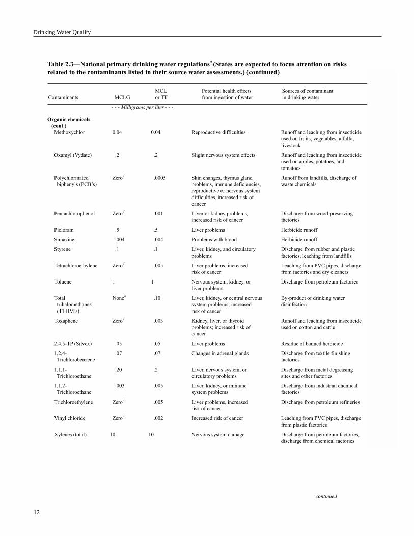
Table 2.3—National primary drinking water regulationsa (States are expected to focus attention on risks
related to the contaminants listed in their source water assessments.) (continued)
MCL Potential health effects Sources of contaminant
Contaminants MCLG or TT from ingestion of water in drinking water
- - - Milligrams per liter - - -
Organic chemicals
(cont.)
Methoxychlor 0.04 0.04 Reproductive difficulties Runoff and leaching from insecticide
used on fruits, vegetables, alfalfa,
livestock
Oxamyl (Vydate) .2 .2 Slight nervous system effects Runoff and leaching from insecticide
used on apples, potatoes, and
tomatoes
Polychlorinated Zerod
.0005 Skin changes, thymus gland Runoff from landfills, discharge of
biphenyls (PCB’s) problems, immune deficiencies, waste chemicals
reproductive or nervous system
difficulties, increased risk of
cancer
Pentachlorophenol Zerod
.001 Liver or kidney problems, Discharge from wood-preserving
increased risk of cancer factories
Picloram .5 .5 Liver problems Herbicide runoff
Simazine .004 .004 Problems with blood Herbicide runoff
Styrene .1 .1 Liver, kidney, and circulatory Discharge from rubber and plastic
problems factories, leaching from landfills
Tetrachloroethylene Zerod
.005 Liver problems, increased Leaching from PVC pipes, discharge
risk of cancer from factories and dry cleaners
Toluene 1 1 Nervous system, kidney, or Discharge from petroleum factories
liver problems
Total Noneb
.10 Liver, kidney, or central nervous By-product of drinking water
trihalomethanes system problems; increased disinfection
(TTHM’s) risk of cancer
Toxaphene Zerod
.003 Kidney, liver, or thyroid Runoff and leaching from insecticide
problems; increased risk of used on cotton and cattle
cancer
2,4,5-TP (Silvex) .05 .05 Liver problems Residue of banned herbicide
1,2,4- .07 .07 Changes in adrenal glands Discharge from textile finishing
Trichlorobenzene factories
1,1,1- .20 .2 Liver, nervous system, or Discharge from metal degreasing
Trichloroethane circulatory problems sites and other factories
1,1,2- .003 .005 Liver, kidney, or immune Discharge from industrial chemical
Trichloroethane system problems factories
Trichloroethylene Zerod
.005 Liver problems, increased Discharge from petroleum refineries
risk of cancer
Vinyl chloride Zerod
.002 Increased risk of cancer Leaching from PVC pipes, discharge
from plastic factories
Xylenes (total) 10 10 Nervous system damage Discharge from petroleum factories,
discharge from chemical factories
continued

13
Chapter 2
Table 2.3—National primary drinking water regulationsa (States are expected to focus attention on risks
related to the contaminants listed in their source water assessments.) (continued)
MCL Potential health effects Sources of contaminant
Contaminants MCLG or TT from ingestion of water in drinking water
- - - Milligrams per liter - - -
Radionuclides
Beta particles and Noneb
4 millirems Increased risk of cancer Decay of natural and man-made
photon emitters per yr deposits
Gross alpha particle Noneb
15 pCi/L Increased risk of cancer Erosion of natural deposits
activity
Radium 226 and Noneb
5 pCi/L Increased risk of cancer Erosion of natural deposits
radium 228
(combined)
Microorganisms
Giardia lamblia Zerod
TT Giardiasis—a gastroenteric Human and animal fecal waste
disease
Heterotrophic plate NA TT No health effects but can NA
count indicate how effective
treatment is at controlling
microorganisms.
Legionella Zerod
TT Legionnaire’s Disease—a Found naturally in water, multiplies
form of pneumonia in heating systems
Total coliforms Zerod
5.0% Used as an indicator that other Human and animal fecal waste
(including fecal potentially harmful bacteria
coliform and may be present
E. coli)
Turbidity NA TT Turbidity has no health effects Soil runoff, growth of algae
but can interfere with disinfection
and provide a medium for
microbial growth. It may indicate
the presence of microbes.
Viruses (enteric) Zerod
TT Gastroenteric disease Human and animal fecal waste
MCL = maximum contaminant level or the maximum permissible level of a contaminant in drinking water delivered to any user;
MCLG = maximum contaminant level goal; NA = not available; pCi = picocuries; PVC = polyvinyl chloride; TT = treatment technique.a Water-quality regulations are subject to change. For the latest regulations, visit the Web site: http://www.epa.gov/OGWDW/wot/appa.html.
b MCLG has not been defined.
c The units vary with the contaminant and are defined by the U.S. Environmental Protection Agency.
d MCLG is 0.0.
Source: U.S. EPA 1999b.

14
Dissolved Gases
The most abundant dissolved gases in water are nitrogen
(N2), oxygen (O
2), carbon dioxide (CO
2), methane (CH
4),
hydrogen sulfide (H2S), and nitrous oxide (N
2O). The first
three are abundant in the Earth’s atmosphere. The second
three are typically products of biogeochemical processes
that occur in nonaerated, low oxygen environments. The
solubility of most gases increases with decreasing water
temperature and decreases with increasing concentrations
of chlorides or other salts.
The concentration of dissolved oxygen (DO) is essential to
aquatic life and can effect the water’s color, taste, odor, and
chemistry. Unpolluted surface waters are generally saturated
with DO because of reaeration and the production of oxygen
during photosynthesis by submerged aquatic plants. Ground
water systems tend toward oxygen depletion and reducing
conditions because the oxygen consumed during
hydrochemical and biochemical reactions is not replenished
by the atmosphere. Polluted surface waters tend to have
lower DO concentrations because of oxygen consumption
during the decomposition of organic matter.
The concentrations of DO strongly influence the solubility
and stability of elements that readily gain or lose electrons
including iron (Fe+3), manganese (Mn+3), nitrogen, sulfur
(S), and arsenic (As+3). When dissolved iron and manganese
are exposed to air, they form insoluble precipitates that
make water turbid, cause stains in laundry, and impart a
bitter taste (Cox 1964). In water with little or no oxygen,
iron minerals are reduced, and adsorbed phosphorus and
other elements can be released into the water. The solubility
of most arsenic and arsenic-sulfur compounds depends on
the presence of DO and can have concentrations in water
above the primary standard of 0.05 milligrams (mg) per liter
(L) (Freeze and Cherry 1979).
Organic Compounds
Organic compounds have carbon and usually hydrogen and
oxygen as the main components in their structural frame-
work. They are typically nonpolar, have relatively low
solubility, and are degraded by microorganisms, hydrolysis,
oxidation-reduction, and volatilization. In natural waters,
they are transported as dissolved phases and attached to
particulates.
Commonly occurring natural organic compounds include
plant and animal tissue and the products of their decomposi-
tion. Synthetic organics found in water include petroleum
products, pesticides, and herbicides (table 2.3). Most
synthetic toxic organic compounds originate from coal
mining, petroleum refining, and manufacture of textile,
wood pulp, and pesticides (table 2.1). In the environment,
they are usually associated with roadways and industrial,
urban, and agricultural land uses. Disinfecting some
organic-rich waters with chlorine may also result in the
formation of carcinogenic organic compounds such as
trihalomethanes (Martin and others 1993, see chapter 5).
Highly soluble, potentially carcinogenic organic compounds
from gasoline spills and emissions are also found in water
supplies and can make water distasteful and undrinkable
(see chapter 6).
Trace Metals and Nonmetals
Primary and secondary water-quality standards have been
developed for common trace metals and nontrace elements
(tables 2.3, 2.4). Most of these elements occur in natural,
uncontaminated waters in concentrations below 1 mg per
liter. Metals have relatively low solubilities. Solubilities are
usually lowest at neutral acidity and increase with increasing
acidity and increasing alkalinity. A characteristic feature of
metals is their tendency to form hydrolyzed species and
Drinking Water Quality
Table 2.4—National secondary drinking water
regulations, which are nonenforceable guidelines for
contaminants that may cause cosmetic effects (e.g., skin
or tooth discoloration) or aesthetic effects (e.g., taste,
odor, or color) in drinking water
Contaminant Unit Secondary standard
Aluminum mg/L 0.05–0.2
Chloride mg/L 250
Color Color units 15
Copper mg/L 1.0
Fluoride mg/L 2.0
Foaming agents mg/L .5
Iron mg/L .3
Manganese mg/L .05
Odor Threshold 3
odor number
pH 6.5 –8.5
Silver mg/L .10
Sulfate mg/L 250
Total dissolved mg/L 500
solids
Zinc mg/L 5
Source: U.S. EPA 1999c.
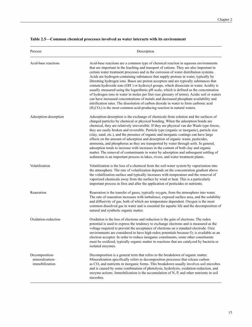
15
Table 2.5—Common chemical processes involved as water interacts with its environment
Process Description
Acid-base reactions Acid-base reactions are a common type of chemical reaction in aqueous environments
that are important in the leaching and transport of cations. They are also important in
certain water treatment processes and in the corrosion of water distribution systems.
Acids are hydrogen-containing substances that supply protons in water, typically by
liberating hydrogen ions. Bases are proton acceptors and are typically substances that
contain hydroxide ions (OH–) or hydroxyl groups, which dissociate in water. Acidity is
usually measured using the logarithmic pH scale, which is defined as the concentration
of hydrogen ions in water in moles per liter (see glossary of terms). Acidic soil or waters
can have increased concentrations of metals and decreased phosphate availability and
nitrification rates. The dissolution of carbon dioxide in water to form carbonic acid
(H2CO3) is the most common acid-producing reaction in natural waters.
Adsorption-desorption Adsorption-desorption is the exchange of chemicals from solution and the surfaces of
charged particles by chemical or physical bonding. When the adsorption bonds are
chemical, they are relatively irreversible. If they are physical van der Waals type forces,
they are easily broken and reversible. Particle type (organic or inorganic), particle size
(clay, sand, etc.), and the presence of organic and inorganic coatings can have large
effects on the amount of adsorption and desorption of organic waste, pesticides,
ammonia, and phosphorus as they are transported by water through soils. In general,
adsorption tends to increase with increases in the content of both clay and organic
matter. The removal of contaminants in water by adsorption and subsequent settling of
sediments is an important process in lakes, rivers, and water treatment plants.
Volatilization Volatilization is the loss of a chemical from the soil-water system by vaporization into
the atmosphere. The rate of volatilization depends on the concentration gradient above
the volatilization surface and typically increases with temperature and the removal of
vaporized chemicals away from the surface by wind or heat. This is a particularly
important process in fires and after the application of pesticides or nutrients.
Reaeration Reaeration is the transfer of gases, typically oxygen, from the atmosphere into water.
The rate of reaeration increases with turbulence, exposed surface area, and the solubility
and diffusivity of gas, both of which are temperature dependent. Oxygen is the most
common dissolved gas in water and is essential for aquatic life and the decomposition of
natural and synthetic organic matter.
Oxidation-reduction Oxidation is the loss of electrons and reduction is the gain of electrons. The redox
potential is used to express the tendency to exchange electrons and is measured as the
voltage required to prevent the acceptance of electrons on a standard electrode. Oxic
environments are considered to have high redox potentials because O2 is available as an
electron acceptor. In order to reduce inorganic constituents, some other constituents
must be oxidized, typically organic matter in reactions that are catalyzed by bacteria or
isolated enzymes.
Decomposition- Decomposition is a general term that refers to the breakdown of organic matter.
mineralization- Mineralization specifically refers to decomposition processes that release carbon
immobilization as CO2 and nutrients in inorganic forms. This breakdown usually involves soil microbes
and is caused by some combination of photolysis, hydrolysis, oxidation-reduction, and
enzyme actions. Immobilization is the accumulation of N, P, and other nutrients in soil
microbes.
Chapter 2

16
Table 2.6—Summary of the chemical behavior of important water contaminants
Biochemical Chemical Physiochemical
transformationsa
reactions retardationb
Contaminant Aerobic Anaerobic Acid Alkaline Acid Alkaline
Metals
Aluminium (Al+3
) M P P D P D
Cadmium (Cd+2
) P P P D P M
Chromium (Cr+3
) P P M P D P
Copper (Cu+1
) P P M D D M
Iron (Fe+3
) D P P D M D
Lead (Pb+4
) P P M D M D
Manganese (Mn+3
) M M P D M D
Mercury (Hg+1
) M P M D M D
Silver (Ag+1
) P P M D M D
Zinc (Zn+2
) P P P D P D
Inorganic nonmetals
Ammonium (NH4+1
) D P P P P D
Nitrate (NO3-1
) P D P P P P
Sodium (Na) P P P P P M
Sulphate (SO4-2
) P D P M P P
Fluoride (F-1
) P P M M D P
Chloride (Cl-1
) P P P P P P
Arsenic (As) P P M P M D
Selenium (Se) P P D M D P
Cyanide P P P P D P
Organic compounds
Aliphatic D P P P D D
Hydrocarbons
Phenols D M P P M M
Benzene D P P P D D
Toluene D P P P D D
Polynuclear
aromatics M P P P M M
Halogenated organics
Tri and tetra
chloroethylene P M P P M M
Carbon tetrachloride P M P P M M
Chloroform P M P P P P
Methylene chloride M M P P P P
Chlorobenzene D P P P D D
Chlorphenols D M P P P M
Fecal organisms
Fecal coliform P P P P M P
Pathogenic bacteria P P P P M P
Pathogenic virus P P D M M D
D = reactions do occur; M = reactions may occur; P = reactions probably occur.a Biochemical transformations involve biological organisms, usually microbes.
b Physiochemical retardation involves physical and chemical bonds that are usually to mineral surfaces.
Source: Adapted and updated from Foster and Gomes 1989.
Drinking Water Quality

17
inorganic and organic complexes. These complexes typi-
cally absorb to suspended particulates or form insoluble
precipitates. Therefore, the transport of metals across the
landscape is often related to acidity, the presence of organic
compounds, and the transport of sediment (table 2.6).
While trace metals and nonmetals occur naturally, their
concentrations can be greatly increased over background
levels by mining activities, waste dumps, acidic runoff,
tanneries, and other industries. Some metals, such as copper
and cadmium, are associated with automobiles and are
concentrated on streets, parking lots, and industrial areas
(Bannerman and others 1993). Major sources of lead include
urban soil, lead-based paint, and some hair-coloring
cosmetics (Mielke 1999).
Fluorine (F) is a trace nonmetal that occurs as fluoride and
is undersaturated in nearly all natural water. Because it can
have beneficial effects on dental health, fluorine is added to
some municipal water supplies. Arsenic is a soluble trace
nonmetal that can be naturally present in water from areas of
recent volcanism. It is widely used in pigments, insecticides,
herbicides, and metal alloys (Freeze and Cherry 1979).
Selenium (Se) is a toxic nonmetallic element that has
geochemical properties similar to sulfur. It can occur in
appreciable concentrations in coal, uranium ore, certain
shales, and discharges from petroleum refineries and mines.
Like sulfur, it forms strong chemical bonds on the surface of
minerals and can be reduced by anaerobic bacteria
(Schlesinger 1997).
Nitrogen
Nitrogen, a major nutrient for vegetation, plays a dominant
role in many biochemical reactions. However, in certain
chemical forms, it can adversely affect humans, ecosystems,
and water supplies. Since preindustrial times, fertilizer
production and other human activities have more than
doubled the global input of nitrogen to terrestrial ecosystems
(Kinzig and Socolow 1994, Vitousek and others 1997). This
increase has made nitrogen the most common water
pollutant in the United States. In the Northeastern United
States alone, anthropogenic activities have apparently
increased the nitrate concentrations in major rivers threefold
to tenfold since the early 1900’s (Matson and others 1997).
Anthropogenic alteration of nitrogen cycles has also affected
forest and aquatic productivity and increased acid rain,
photochemical smog, and greenhouse gases (Fenn and
others 1998, Vitousek and others 1997).
Certain nitrogen compounds can have toxic effects at
relatively low concentrations. Methaemoglobinemia (blue-
baby syndrome) in bottle-fed babies and the elderly is a
human health hazard associated with nitrite (NO2
-1) indrinking water (table 2.2). Nitrate in water can also present
similar health hazards as can nitrate in many foods (GEMS
1991). Bacteria residing in vertebrate digestive tracts can
convert the relatively benign nitrate into the toxic nitrite
(Kinzig and Socolow 1994). Ammonia dissolved in drinking
water is not toxic to humans but can be toxic to some
aquatic invertebrates and fish depending on the concentra-
tion of DO temperature, acidity, and salinity, and the carbon
dioxide-carbonic acid equilibrium of water. Because all
forms of inorganic nitrogen are nutrients to green plants,
excessive concentrations in water can lead to algal blooms,
excessive growth of submerged aquatic plants, and eutrophi-
cation, particularly in coastal and marine ecosystems.
The global nitrogen cycle consists of three major reservoirs:
(1) the atmosphere, (2) the hydrosphere, and (3) the bio-
sphere (fig. 2.1). The flow between these reservoirs occurs
in many forms and pathways (fig. 2.2). Inorganic nitrogen
can be transported in water as dissolved nitrous oxide or
nitrogen gas, ammonia, and cations or as anions of nitrite or
nitrate. The concentrations of these compounds are low in
most unpolluted freshwater and high in waters contaminated
by organic wastes, sewage, or fertilizers. Worldwide,
pristine rivers have average concentrations of ammonia and
nitrate of 0.015 mg per liter and 0.1 mg per liter, respec-
tively (GEMS 1991). Nitrate concentrations > 1 mg per liter
generally indicate anthropogenic inputs. The lowest concen-
trations are generally found in deep ground water and
surface waters draining pristine wildlands (GEMS 1991,
Spahr and Wynn 1997). The highest levels are associated
with surface runoff and ground water from fertilized
agricultural and urban areas. In undisturbed watersheds,
annual yields increase with annual runoff, and yields from
savanna and rangeland are less than from forest (Lewis and
others 1999).
Organic nitrogen is converted to inorganic nitrogen in a
process called mineralization in the following oxidation
sequence: organic nitrogen and ammonium to nitrite to
nitrate. In water that is strongly oxidized, nitrate is the stable
phase and is very mobile. As redox potential declines,
nitrate is reduced or denitrified to nitrous oxide or nitrogen
gas. Because of the potential adverse ecosystem and health
effects associated with nitrites and nitrates, denitrification is
desirable for water quality. Generally, the amount of net
mineralization is directly related to the total content of
organic nitrogen and carbon (Schlesinger 1997, Vitousek
and Melillo 1979). Nitrification tends to be lower in soil
with low acidity, low soil oxygen, low soil moisture, and
low temperature, and high litter carbon to nitrogen ratios. At
the watershed scale, rates of denitrification vary with
landscape positions (Jordan and others 1993, Peterjohn and
Chapter 2

18
Figure 2.1—Global nitrogen cycle. Annual fluxes in units of 1012
grams per year.
Correll 1984). In general, relatively high denitrification rates
are found in riparian forests and at the base of slopes where
water, carbon, nitrogen, and phosphorus are readily
available.
Because nitrogen is essential to the growth of plants,
seasonal differences in plant uptake can cause measurable
variations in the concentration of nitrogen in soil and
surface water. In general, the lowest nitrogen levels in
surface or ground water occur during the early growing
season when plant uptake is greatest (Boyd 1996). Maxi-
mum nitrogen concentrations typically occur in the winter
when plant uptake is reduced, and the dissolved fraction is
concentrated in unfrozen water. However, seasonal trends
can be reversed or diminished in areas with large
anthropogenic inputs.
Phosphorus
The presence of phosphorus in drinking water is not
considered a human health hazard, and no drinking water-
quality standards are established for phosphorus. Neverthe-
less, phosphorus can affect the water’s color and odor and
indicate the presence of other organic pollution. Further-
more, because phosphorus can accelerate the growth of
algae and aquatic vegetation, it contributes to the eutrophi-
cation and associated deterioration of municipal water
supplies. Whereas excess nitrogen is responsible for most of
Drinking Water Quality
Land
plants
100
Human
activities
Atmosphere
Denitrification
110
Biological
fixation
15
The Global Nitrogen Cycle
Internal
cycling
Ground water
Soil organic - N
Internal
cycling
Oceans
Biological
fixation
140
1200
Denitrification
≤ 200
Permanent
burial
10
8000
River
flow
36
30
Fixation in
lightning
< 3

19
Chapter 2
Figure 2.2—Sources and pathways of nitrogen in the subsurface environment.
Organic - N
proteins
N2 N2
Denitrification
Decompositionnitrification
Adsorption
Proteins
water
Precipitation
Mineral
fertilizerSewagePlant residue,
compost
Plantproteins
Nitrification
Nitrogenfixation
Denitrification
Denitrification in reducing zones
Decomposition
Nitrification
Denitrification
Adsorption
N2
{ }
NH3
NO-3
NH3
NO-3
NO-3
NH3Organic - N
NH3
NH3N2
NH+4
NO-3
NO-3
NH+4
NO-3NO-
3
NH+4
N2
NH+4
Leaching
N2(aq) N20
NO-3
NO-3
NO-3
Ground

20
the coastal and marine eutrophication, agricultural sources
of phosphorus dominate the eutrophication processes in
many freshwater aquatic systems (Matson and others 1997).
Nearly all the phosphorus in terrestrial ecosystems is
originally derived from the weathering of minerals (fig. 2.3).
The most common phosphorus-rich mineral is apatite, a
calcium orthophosphate that is present in some igneous
rocks and marine sediments. In natural freshwater, phospho-
rus exists in both dissolved and particulate fractions.
Dissolved phases typically originate from excretions by
organisms, whereas particulate fractions can have organic or
inorganic origins. In streams, a large fraction of phosphorus
is adsorbed on and transported with organic and inorganic
particulates. In lakes, a large proportion of the phosphorus in
oxygen-rich surface waters is held in plankton biomass
(Schlesinger 1997). In deeper, anoxic lakes, phosphorus is
adsorbed to sediments and particulates but can be released
during the reduction of iron compounds. Unlike nitrogen,
carbon, and hydrogen, phosphorus does not have a signifi-
cant gaseous component.
Chemical Evolution of Water
As water moves across the landscape, it interacts with the
surfaces it contacts and chemically evolves toward the
composition of seawater [for detailed explanations see
Stumm and Morgan (1970) and Freeze and Cherry (1979)].
In general, the evolution of deep ground water typically
involves increases in dissolved solids and decreases in DO,
organic waste, pesticides, phosphorus, and nitrogen. In
contrast, the concentrations of organic waste, pesticides,
phosphorus, and nitrogen increase as surface water travels
across the landscape and interacts with both natural and
anthropogenic systems.
Fresh, young water that has had little contact with its
surroundings is generally low in total dissolved solids and
rich in bicarbonate anions derived from soil carbon dioxide
and the dissolution of carbonate minerals. Sulfate anions
tend to dominate in intermediate age ground water while
chloride anions dominate in older, deep ground water that
has traveled long distances. These sulfate and chloride
anions are derived from the dissolution of soluble sedimen-
tary minerals. Because these minerals are present only in
small amounts in most rocks, water usually has to travel
considerable distances before it is dominated by either
sulfate or chloride anions.
The DO content and redox potential tend to decrease as
water travels across the landscape. Rain and snow are
exposed to atmospheric oxygen and have relatively high DO
and redox potentials. As water passes through organic-rich
forest litter and soil, the DO is removed, redox potential
declines, and large amounts of organic acids are generated.
Nutrient immobilization predominates in the upper layers of
fresh litter, while mineralization of nitrogen, phosphorus,
and sulfur is usually greatest in the upper mineral soil. As
water travels through the subsurface, all the DO is con-
sumed by bacterially catalyzed reactions that oxidize
organic matter. Eventually the aerobic bacteria involved in
these reactions can no longer thrive, and anaerobic condi-
tions prevail. Then ammonia, manganese, ferrous iron, and
sulfate become oxidizing agents.
Cation concentrations in water vary considerably in space
and time and do not follow well-defined, theoretically based
sequences like anions or redox potentials. Nevertheless,
cations enter the aquatic system from the weathering of
minerals and the breakdown of organic materials. Their
concentrations typically increase with travel distance in both
surface and ground water. The most abundant cations in
water supplies are calcium and magnesium, which can be
removed by chemical treatments to prevent scaling of pipes
and to reduce the amount of soap needed for washing.
Physical Properties
The physical characteristics of concern in drinking water are
temperature, color, turbidity, sediments, taste, and odor.
Temperature
Because of its hydrogen bonds and molecular structure,
water has an unusual trait—the density of its solid phase
(ice) is lower than that of its liquid phase (water). Because
of this trait, ice floats, and pipes and plant tissues rupture
when the water within them freezes and expands.
The rates of chemical and metabolic reactions, viscosity and
solubility, gas-diffusion rates, and the settling velocity of
particles depend on temperature. Metabolism, reproduction,
and other physiological processes of aquatic organisms
are controlled by heat-sensitive proteins and enzymes
(Ward 1985). A 10 °C increase in temperature will roughly
double the metabolic rate of cold-blooded organisms and
many chemical reactions. A permanent 5 °C change in
temperature can significantly alter the structure and compo-
sition of an aquatic population (MacDonald and others
1991, Nathanson 1986). Temperature increases also de-
crease DO concentrations but can increase the oxidation rate
and efficiency of certain biological, wastewater treatment
systems.
Drinking Water Quality

21
Figure 2.3—Global phosphorus cycle. Annual fluxes in units of 1012
grams per year.
Chapter 2
The temperature of water naturally varies with time of day,
season, and the type of water body. Changes in surface
water temperatures reflect seasonal changes in net radiation,
daily changes in air temperature, and local variations in
incoming radiation. Temperature variations in ground water
are less than in surface water. Except in the winter, surface
water is usually warmer than ground water, and most
anthropogenic activities increase water temperatures.
Removal of vegetative canopies over streams influences
water temperatures by affecting energy inputs, evaporative
cooling, and the way water flows across the landscape. The
cooling rate for surface water depends on heat transfer to the
atmosphere.
Seasonal and spatial variations in the temperature in water
supply reservoirs can have large effects on the quality of
raw municipal water (Cox 1964). Water in deep reservoirs is
commonly divided into three zones: the upper circulating
zone, the middle transition zone, and the deepest zone of
stagnation. Water in the upper surface zone is aerated and
mixed by wind action and typically has abundant DO. In
contrast, the deepest, stagnant water contains little or no DO
because it has been removed during the oxidation of organic
matter. The breakdown of organic matter also makes deep
water acidic and rich in carbonic acid. Consequently,
stagnate, deep water has the chemical conditions necessary
to dissolve iron, manganese, sulfur, and other taste- and
odor-producing substances. To avoid the objectionable taste
and odor of the deep water, municipal water is usually
drawn from the surface of the reservoir. However, when the
temperature of the surface water falls rapidly, it can become
denser than the bottom water, causing the entire water
column of the reservoir to mix or “turn over.” During these
mixing events, the DO content of the entire lake can
decrease, causing massive fish kills and foul smelling and
poor tasting water. Similar mixing can occur in stratified
lakes or estuaries during periods of intense runoff.
Color and Turbidity
Pure water is colorless in thin layers and bluish green in
thick layers. Particulates and insoluble compounds typically
add color and reduce transparency. Consequently, the
presence of light-dependent aquatic organisms can affect
esthetic appeal and taste of water as well as the effectiveness
of certain wastewater treatment processes.
60
Soils
200,000
Internal
cycling
Mining
Mineable
rock
10,000
Riverflow
Reactive
Bound
Dust transport
The Global Phosphorus Cycle
Internal
cycling
90,000
Sediments
4.0 x 10⁹
12
1.0
1000
2
19
2
Land plants
3,000

22
Turbidity is an optical property related to the scattering of
light and clarity. It is typically controlled by the presence of
suspended particles or organic compounds. Turbidity itself
is not injurious to human health. Approximately 50 percent
of the total incident light is scattered or transformed into
heat within the first meter of water. As turbidity increases, it
reduces the depth of sunlight penetration, thereby altering
water temperature and stratification, the photosynthesis of
aquatic organisms, the DO content of the water body, and
the cost of water treatment. In addition, turbid water can
contain particulate of soil or fecal matter that harbors
microorganisms and/or carries absorbed contaminants. The
removal of particulates by gravity or by addition of chemi-
cals is typically the first step in treating water for human
consumption. The sedimentation of particles and the
bleaching action of sunlight during reservoir storage can
reduce both the color and turbidity of water (Cox 1964).
Sediment
Sediment is a major water-quality concern because of its
ability to transport harmful substances and its impacts on the
cost of water treatment and the maintenance of water
distribution systems. While sediment is derived during the
natural weathering and sculpturing of the landscape,
accelerated levels of erosion and sedimentation are associ-
ated with many anthropogenic activities (table 2.1).
The general term sediment includes both organic and
inorganic particles that are derived from the physical and
chemical weathering of the landscape. Individual particles
are eroded, transported, and deposited. Erosion can be either
physical or chemical. Transport can be by wind, gravity, or
water. In water and air, particles can be transported in
suspension (suspended load) or along the substrate (bed
load). Sediment load is the total quantity of sediment that is
transported through a cross-section of a stream during a
specific time period. The actual amount of sediment
transported at any place or time depends on the supply of
sediment and the transport capacity of the stream. Sediment
is usually measured as mass per unit area (tons per acre per
year or metric tonnes per hectare per year), concentration
(parts per million or milligrams per liter), or lowering of the
landscape (inches per 1,000 years or millimeters per 1,000
years). In general, high sediment loads increase water
treatment costs and reduce the storage volume and life span
of water storage facilities.
Biological Properties
Aquatic organisms are usually grouped into those that
(1) obtain the carbon they need for biosynthesis from carbon
dioxide (autotrophs) and (2) use existing organic com-
pounds as their carbon source (heterotrophs). Generally,
autotrophs increase DO concentrations in water through
photosynthesis, while heterotrophs are responsible for
breakdown and recycling of dead organic materials and
decreased DO concentrations.
Most microbial contaminants in water are caused by
heterotrophs that are transmitted to a water system via
human and animal fecal matter (U.S. EPA 1999a). Most
waterborne pathogenic microorganisms are bacteria or
viruses that survive in sewage and septic leachate (table
2.7). Bacterial pathogens are generated by both animal and
human sources, while viral pathogens are usually only
generated by human sources. Viruses that infect animals
normally do not cause illness in humans. However, animal
sources for some viruses that effect humans are suspected,
particularly viruses that infect the respiratory system like the
sin nombre virus, hantavirus, influenza virus, and Ebola
virus.
Common bacterial diseases spread by aquatic microorgan-
isms include Legionnaire’s disease, cholera, typhoid, and
gastroenteritis. Waterborne viral diseases include polio,
hepatitis, and forms of gastroenteritis. Waterborne parasitic
diseases include amoebic dysentery, flukes, and giardiasis.
Giardia spp. and Cryptosporidium spp. are parasitic
protozoans that are transferred between animals and humans
via the fecal-oral route and are significant sources of
gastrointestinal illness. They are common in surface water in
back-country areas, including in many national forests and
parks. These back-country areas, which provide animal
habitat, experience low human use (Monzingo and Stevens
1986) (see chapter 15). Unfortunately, some parasitic
protozoans are not removed in most water treatment plants
because they are small enough to pass filtration systems and
are very resistant to disinfectants.
The analytical procedures for detecting waterborne viral
diseases are costly and time consuming. Therefore most
drinking and recreational waters are routinely tested for
microbes that are easier to detect but whose presence is
highly correlated with human health hazards. Coliforms are
the most common type of microbes used in this type of
testing. All coliforms are aerobic and facultative anaerobic,
gram-negative, nonspore-forming, rod-shaped bacteria that
ferment lactose. Their presence and abundance in raw water
is used to screen for fresh fecal contamination (Cox 1964).
Their presence in treated water is used to determine treat-
ment plant efficiency and the integrity of the distribution
system.
Many environmental factors can affect the transport of
microbes across the landscape (table 2.8). Relatively
Drinking Water Quality

23
Table 2.7—Common waterborne pathogenic and indicator bacteria and viruses
Waterborne pathogenic bacteria Waterborne pathogenic viruses
Legionella
Mycobacterium avium intracellular (MAC)
Shigella (several strains)
Helicobacter pylori
Vibrio cholerae
Salmonella typhi
S. typhimurum
Yersinia
Campylobacter (several strains)
Escherichia coli (several pathogenic strains)
Waterborne indicator bacteria Waterborne indicator viruses
Total coliform
Fecal coliform
E. coli (both nonpathogenic and
pathogenic strains)
Enterococci
Fecal streptococci
Clostridium perfringens (anaerobic spores)
Klebsiella pneumoniae
Aeromonas hydrophila
Source: U.S. EPA 1999a.
Chapter 2
coarse-grained or sandy soils are poor adsorbers of microbes
(Keswick and Gerba 1980, U.S. EPA 1999a). Fine-textured
clay soils or soils with abundant colloidal organic material
are very adsorbent because their negatively charged surfaces
and large surface area per-unit volume increase the number
of potential adsorption sites for microbial contaminants. As
a result, clay soils slow the migration but can enhance the
survival of certain microbes (Bitton and others 1986,
Keswick and Gerba 1980). In contrast, the absorption of
viruses to organic soils or in environments with high
concentrations of dissolved organic matter or organic acids
is relatively poor, probably because of competition for
adsorption sites. The presence of humic and fulvic acids
may reduce virus infectivity.
The acidity and ionic strength of liquids percolating past
adsorbed microbes can influence their sorption and desorp-
tion. Moreover, a reduction in the ionic strength of pore
water weakens the virus-soil adsorption forces and increases
their entrainment and concentrations in percolating water
(Bitton and others 1986). Therefore, natural rainwater with
its extremely low ionic strength can mobilize and transport
viruses that have sorbed to the upper layers of the soil.
Fecal contamination of surface and ground water can occur
by several pathways (table 2.1). The concentration of
microbes in surface runoff is generally higher in warmer
months and higher in runoff from grazed rather than
ungrazed land (Edwards and others 1997). Lawns and
residential streets are important sources of fecal coliforms
from domestic animals (Bannerman and others 1993).
Leaking sewer lines and failed septic systems are also
common sources (U.S. EPA 1999a), and water distribution
systems can harbor bacterial or fecal contamination. This
contamination enters distribution systems when controls fail
or when negative pressure in a leaking pipe allows contami-
nants to infiltrate.
Storage in reservoirs can increase or decrease the microbial
content of surface water. Sedimentation of particles with
adsorbed microbes and the germicidal action of sunlight can
lower microbial content (Cox 1964). However, these effects
are spatially and seasonally variable and are influenced by
microclimate and the morphology and chemistry of a water
body (James and Havens 1996). Eutrophic conditions that
reduce DO concentrations or produce toxic blue-green algae
blooms may decrease water quality (see Hebgen Lake case
in chapter 5).
Bacteriophage
Bacteroides phage
Coliphage
Male-specific coliphage
FRNA phage
FDNA phage
Host Salmonlla WG-49
Host E. coli C-3000
Host E. coli FAMP
Host E. coli 15597
Somatic coliphage
Host E. coli C 13706, C-3000
Host Salmonella WG-49
Enteroviruses
Coxsackieviruses
Echoviruses
Poliovirus
Enterovirus 70 and 71
Hepatitis A virus
Hepatitis E virus
Enteric adenoviruses
Rotavirus
Norwalk virus
Small round structured viruses (SRSV)
Astrovirus
Caliciviruses

24
Drinking Water Quality
Table 2.8—Factors influencing virus transport and fate in the subsurface
Factor Influence on fate of virus Influence on transport
Light Minor factor in virus inactivation, effective only at Unknown
the soil’s surface
Temperature Viruses survive in soil and water longer at lower Unknown
temperatures.
Hydrogeologic A short ground water time of travel indicates that Relatively slow flow reduces the rate
conditions and well viruses may be transported to water supply wells of virus migration while conduit,
pumping rate before dying off or becoming inactivated. High fracture flow, or rapid flow in coarse-
pumping rates decrease ground water travel times. grained, porous media enhances
transport.
Soil properties; iron- Effects on survival are probably related to the degree High degree of virus retention by the
oxide coatings on of virus adsorption. Iron oxides probably increase clay fraction of soil; iron coatings
soil or aquifer grains inactivation. may be especially efficient in
providing an attractive surface for
virus attachment.
pH Most enteric viruses are stable between a pH range Generally, low pH favors virus
of 3 to 9. Survival may be prolonged at near-neutral adsorption and high pH results in
pH values. virus desorption from particles.
Inorganic ions/salt Some viruses are protected from inactivation by Generally, increasing the concentration
species and certain cations; the reverse is also true. of ionic salts and increasing cation
concentration valencies enhance virus adsorption.
Organic matter Presence of organic matter may protect viruses from Soluble organic matter competes with
inactivation; others have found that it may reversibly viruses for adsorption sites on soil
retard virus infectivity. particles.
Virus type Different virus types vary in their susceptibility to Virus adsorption to soils is probably
inactivation by physical, chemical, and biological related to physicochemical differences
factors. in virus capsid surfaces.
Microbial activity Some viruses are inactivated more readily in the Unknown
presence of certain microorganisms; however,
adsorption to the surface of bacteria can be
protective.
Iron content in May increase virus attachment and inactivation Iron-oxidizing bacteria may form a
shallow soil or biomass layer that filters out viruses.
aerobic aquifers Heavy precipitation events may cause
the ionic strength of the water to
decline and the biofilms to release the
filtered organisms.
Soil moisture Influences inactivation and adsorption to particle Increased saturation promotes
content surfaces; survival may increase in unsaturated desorption of viruses from particle
conditions. surfaces and migration in
ground water.
Source: U.S. EPA 1999a.

25
Literature Cited
Bannerman, R.; Owens, D.; Dodds, R.; Hornewer, N. 1993. Sources of
pollutants in Wisconsin stormwater. Water Science and Technology.
28(3–5): 241–259.
Bitton, G.; Farrah, S.R.; Montague, C.L.; Akin, E.W. 1986. Viruses in
drinking water. Environmental Science and Technology. 20(2): 216–222.
Boyd, R.A. 1996. Distribution of nitrate and orthophosphate in selected
streams in central Nebraska. Water Resources Bulletin. 32(6):
1247–1258.
Cox, C.R. 1964. Operation and control of water treatment processes.
Geneva: World Health Organization. 390 p.
Edwards, D.R.; Coyne, M.S.; Vendrell, P.F. [and others]. 1997. Fecal
coliform and streptococcus concentrations in runoff from grazed
pastures in northwest Arkansas. Water Resources Bulletin. 33(2):
413–422.
Fenn, M.E.; Poth, M.A.; Aber, J.D. [and others]. 1998. Nitrogen excess
in North America ecosystems: predisposing factors, ecosystem
responses, and management strategies. Ecological Applications. 8(3):
706–733.
Foster, S.; Gomes, D.C. 1989. Groundwater quality monitoring: an
appraisal of practices and costs. Lima, Peru: Pan American Center for
Sanitary Engineering and Environmental Sciences. 103 p.
Freeze, R.A.; Cherry, J.A. 1979. Groundwater. Englewood Cliffs, NJ:
Prentice-Hall, Inc. 604 p.
GEMS. 1991. Freshwater pollution. UNEP/GEMS Environment Library 6.
[Place of publication unknown]: [Publisher unknown]. 36 p.
James, T.R.; Havens, K.E. 1996. Algal bloom probability in a large
subtropical lake. Water Resources Bulletin. 32(5): 995–1006.
Jordan, T.E.; Corell, D.L.; Weller, D.E. 1993. Nutrient interception by a
riparian forest receiving inputs from adjacent cropland. Journal of
Environmental Quality. 22: 467–473.
Keswick, B.H.; Gerba, C.P. 1980. Viruses in ground water. Environmental
Science and Technology. 14(11): 1290–1297.
Kinzig, A.P.; Socolow, R.H. 1994. Human impacts on the nitrogen cycle.
Physics Today. November: 24–31.
Lewis, W.M., Jr.; Melack, J.M.; McDowell, W.H. [and others]. 1999.
Nitrogen yields from undisturbed watersheds in the Americas.
Biogeochemistry. 46: 149–162.
MacDonald, L.H.; Smart, A.W.; Wissmar, R.C. 1991. Monitoring
guidelines to evaluate effects of forestry activities on streams in the
Pacific Northwest and Alaska. U.S. EPA 910/9–91–001. 166 p. Available
from: U.S. Environmental Protection Agency, Region 10, NPS Section,
WD–139, 1200 Sixth Avenue, Seattle, WA 98101.
Martin, A.B.; Cooke, G.D.; Carlson, R.E. 1993. Lake sediments as
potential sources of trihalomethane precursors. Water Resources
Research. 27(12): 1725–1729.
Matson, P.A.; Parton, W.J.; Power, A.G.; Swift, M.J. 1997. Agricultural
intensification and ecosystem properities. Science. 77: 504–509.
Mielke, H.W. 1999. Lead in the inner cities. American Scientist. 87: 62–73.
Monzingo, D.L.; Stevens, D.R. 1986. Giardia contamination of surface
waters: a survey of three selected backcountry streams in Rocky
Mountain National Park. Water Resour. Rep. 86–2. Fort Collins, CO:
National Park Service; Colorado State University. 18 p.
Nathanson, J.A. 1986. Basic environmental technology. Engelwood Cliffs,
NJ: Prentice-Hall, Inc. 479 p.
National Research Council. 1997. Technologies for the small system. In:
Safe water from every tap. Improving water services to small communi-
ties. Water Science and Technology Board. Washington, DC: National
Academy Press: 48–115.
Peterjohn, W.T.; Correll, D.L. 1984. Nutrient dynamics in an agricultural
watershed: observations on the role of a riparian forest. Ecology. 65:
1466–1475.
Schlesinger, W.H. 1997. Biogeochemistry an analysis of global change.
2d ed. New York: Academic Press. 588 p.
Spahr, N.E.; Wynn, K.H. 1997. Nitrogen and phosphorus in surface
waters of the Upper Colorado River Basin. Journal of the American
Water Resources Association. 33(3): 547–560.
Stumm, W.; Morgan, J.J. 1970. Aquatic chemistry. 2d ed. New York: John
Wiley. 583 p.
U.S. EPA. 1999a. Groundwater rule. [Not paged]. [Available on the Web
at: http://www.epa.gov/OGWDW/].
U.S. EPA. 1999b. National primary drinking water regulations. Primary
drinking water standards. [Not paged]. [Available on the Web at: http://
www.epa.gov/OGWDW/wot/appa.html].
U.S. EPA. 1999c. National secondary drinking water regulations. [Not
paged]. [Available on the Web at: http://www.epa.gov/OGWDW/wot/
appa.html].
Vitousek, P.M.; Melillo, J.M. 1979. Nitrate losses from disturbed forests:
patterns and mechanisms. Forest Science. 25: 605–619.
Vitousek, P.M.; Mooney, H.A.; Lubchenco, J.; Melillo, J.M. 1997.
Human domination of the Earth’s ecosystem. Science. 277: 494–499.
Ward, J.V. 1985. Thermal characteristics of running waters. Hydrobiologia.
125: 31–46.
Chapter 2

26
Chapter 3
Watershed Processes—Fluxes of Water,
Dissolved Constituents, and Sediment
F.J. Swanson, F.N. Scatena, G.E. Dissmeyer, M.E. Fenn,
E.S. Verry, and J.A. Lynch1
The Integrated Hydrologic System
Ecosystems are energy-processing units that are continually
cycling and being regulated by essential nutrients and water.
Some cycles, like the hydrologic cycle, are global and, thus,
involve transport over great distances. Other cycles occur
locally among biotic elements, forest litter, and soil. In most
forests, large pools of tightly bound, relatively unavailable
nutrients are linked with small pools of available nutrients
that are rapidly cycled through the ecosystem.
The circulation of water through the hydrologic cycle is the
largest movement of a chemical substance at the surface of
the earth (Schlesinger 1997). The hydrologic cycle describes
the constant exchange of water among the land, sea, and
atmosphere. A water budget is the balance of inflows,
outflows, and changes in storage over a defined time period
at a specific location. Both water cycles and budgets
consider water in solid, liquid, or gaseous form and are
typically viewed in a sequence from precipitation to
streamflow (fig. 3.1). Since most chemicals are somewhat
water soluble, the hydrologic cycle strongly influences
nutrient cycling, weathering, chemical and sediment
transport, and water quality. Furthermore, water plays vital
roles in mobilization and transport of sediment downslopes
and through stream networks.
The basic equation that describes a hydrologic budget is
Q = P - I - T - E - G - W + R + /- S ,
where
Q = streamflow,P = precipitation,
I = interception,
T = transpiration,
E = evaporation,
G = ground water recharge,
W = water withdrawals for consumptive use,R = return flow from outside sources, and
S = change in storage over measurement period.
Introduction
The quantity and quality of drinking water coming from a
watershed depend on processes involving surface water,
ground water, biogeochemistry, biota, atmospheric deposi-
tion, and sedimentation. Quality of drinking water supplies,
therefore, hinges on understanding of the routing of water,
its dissolved constituents, and its entrained sediments
through watersheds and ground water systems (Dunne and
Leopold 1978). Fluxes and storages of water, chemical
constituents, and sediment can be described in terms of the
average properties and variability of the cycling systems
involved. Natural forces, such as floods, can cause changes
in water flows and water quality. At times these changes can
overwhelm effects of land-use practices. It is important,
therefore, to understand natural variability of water systems
in order to have realistic expectations about the quantity and
quality of water yields from specific watersheds. Further-
more, natural variation in streamflow and water quality is
integral to the health of aquatic ecosystems (Poff and others
1997) and, thus, must be considered when attempting to
balance consumptive uses with environmental protection.
In this chapter, we provide general background information
on hydrology, dissolved constituents, atmospheric deposi-
tion, sedimentation, nitrogen impacts of surface and ground
water, cumulative watershed effects of land uses, manage-
ment and policy implications, research needs, and, finally,
key points. This information is useful in assessing drinking
water issues.
1 Ecosystem Team Leader, USDA Forest Service, Pacific NorthwestResearch Station, Corvallis, OR; Ecosystem Team Leader, USDA ForestService, International Institute of Tropical Forestry, Río Piedras, PR;Consultant, Water Quality Management–Nonpoint Source, Eatonton, GA;Research Plant Pathologist, USDA Forest Service, Pacific Southwest ForestExperiment Station, Forest Fire Laboratory, Riverside, CA; Research ForestHydrologist, USDA Forest Service, North Central Experiment Station,Grand Rapids, MN; and Professor of Forest Hydrology, Pennsylvania State
University, University Park, PA, respectively.

27
Units in the equation are expressed in terms of volume or
depth per-unit time (million gallons or liters per day or
inches or centimeters per year). Like all budgets, the
magnitudes of the components depend on the spatial and
temporal scale considered, and their evaluation involves
errors due to measurement and interpretation. Water budgets
for small watersheds typically have combined measurement
errors of 20 percent or greater (Winter 1981). Likewise,
municipal water that is not accounted for, that is, the
difference between the amount of water produced by
treatment plants and the amount legitimately consumed, is
commonly 20 to 40 percent of total water treatment plant
production (World Bank 1993). This difference includes
leakage from the storage and distribution system and
illegitimate uses.
For ease of communication, each component is discussed
below. However, it is important to recognize that compo-
nents are tightly coupled; that is, ground water and surface
water systems, as well as atmospheric and biotic influences
on them, must be viewed and managed as a single system
and a single resource (Winter and others 1998). Many of our
past and present water-use practices and policies have
Figure 3.1—Hydrologic cycle within a watershed.
ignored these linkages. Modification in one part of the
system is likely to significantly affect other parts.
Precipitation and Atmospheric Deposition
Precipitation is often classified by physical form (liquid,
solid, or gas), size (rain, drizzle, or mist), the responsible
weather system (cyclonic, warm front, cold front, convec-
tive, or orographic, etc.), and chemistry (acidic). In general,
the amount of annual precipitation varies with elevation and
aspect relative to the prevailing winds.
Because the water molecule is dipolar and attracts other
molecules, natural precipitation contains dissolved gases in
amounts proportional to their concentrations in the atmo-
sphere, their solubility, and ambient temperature. Uncon-
taminated precipitation also has low concentrations of
solutes, is slightly to moderately acidic, and has a high
redox potential. The equilibrium pH for nonsaline water in
contact with atmospheric carbon dioxide is 5.7; and rain-
water and melted snow in nonurban, nonindustrial areas
typically have pH levels between 5 and 6 (Freeze and
Chapter 3
Subsurface flow systemGround water discharge
Streamflow
Exfiltration
Ground water recharge
Evapotranspiration
Overland flow
Channel flow Precipitation
Water table
Infiltration
Unsaturated
(soil moisture) zone
Saturated
(ground water) zone
Equipotential lines Flowlines

28
Watershed Processes—Fluxes of Water, Dissolved Constituents, and Sediment
Some people in the Eastern United States use cisterns,
shallow wells, or ponds for their water supply. Some sites in
coal regions can use only cistern water sources because
local ground water is extremely acidic (pH < 4.0) from acid
mine drainage. The sites at risk are those where precipitation
pH is < 4.5, and where surface soils do not contain enough
bases (calcium and magnesium bicarbonates) to neutralize
the precipitation acidity. Granitic bedrock, base-poor quartz
sandstones, and sandy soils derived from them have low
amounts of neutralizing bases. Basaltic rocks, sandstones
with high amounts of calcite cement, and marine, sedimen-
tary rocks have high amounts of neutralizing bases. In areas
with acidic source water, public water supplies often adjust
pH as part of the water purification treatment, but this may
not occur in some small, private drinking water systems.
Areas in the United States where precipitation pH averages
< 4.5 are restricted to the Upper Midwest and Eastern United
States (fig. 3.2). Areas with acid surface soils are in the East,
Southeast, Upper Midwest, and Northwest (fig. 3.3). These
soils correspond to areas where lakes and streams are acid,
and, thus, shallow ground water is assumed to be acid
(Church 1983).
Cherry 1979, Park 1987). In contrast, rainfall contaminated
by urban or industrial inputs can frequently have a pH as
low as 3 to 4. This acid rain is typically a result of nitrate
(NO3
-1) and sulfate (SO4
-2) that are derived from the incorpo-
ration of gaseous pollutants in raindrops (Schlesinger 1997).
This increased acidity can increase the rate of weathering
and release of cations from exchange sites. Consequently,
the concentrations of metals in source water and the
corrosion of water storage and distribution systems also
increase, causing higher metal concentrations in drinking
water (McDonald 1985, Park 1987). The constituents of
concern are high acidity levels (pH < 4.5) in precipitation,
high nitrate in soil or ground water, and the interaction of
these in soil water to yield high concentrations of aluminum
(Al) and lead (Pb). In addition, highly acidic water can
dissolve lead in solder joints where copper pipes are used
for plumbing.
Atmospheric deposition is a primary source of mercury (Hg)
that can cause adverse health effects. The dangerous form,
methyl mercury, is bioconcentrated in fish that must be
eaten to endanger health. Methyl mercury in precipitation or
surface waters usually does not occur at toxic concentrations
(Nriagu and Pacyna 1988) (see chapter 2; tables 2.3, 2.4).
pH lab
≥5.35.1–5.34.9–5.14.7–4.94.5–4.74.3–4.5
<4.3
Sites not pictured:
Alaska 03 5.3Puerto Rico 5.1
Figure 3.2—Average acidity (pH) of precipitation in the United States from 1988 through 1997 (National Atmospheric Deposition Program 1999).

29
Evaporation, Transpiration, and Evapotranspiration
Evaporation is the process of converting water from a liquid
or solid state to a gaseous state. Evaporation occurs from
lakes and wetlands, large rivers, soil surfaces, and accumu-
lations of water on vegetative matter or other surfaces.
Sublimation is evaporation from snow and ice surfaces. The
rate of evaporation depends primarily on solar radiation,
temperature, wind, and the humidity gradient above the
evaporating surface. Because evaporation losses from open
water can be large, efforts have been made to reduce losses
from municipal water supplies by covering reservoirs or
storage tanks, using underground storage, controlling
aquatic growth, reducing surface area, and applying chemi-
cals (Viessman and others 1977).
Transpiration is the process by which water is released as
vapor from plants through leaves to the atmosphere and is
influenced by soil moisture, the type of vegetation, vapor
pressure gradients across leaf surfaces, and the same factors
that affect evaporation: solar radiation, temperature,
humidity, and wind. In many cases, evaporation and
transpiration are summed and reported as one process,
termed evapotranspiration (ET). Unlike other pathways, ET
returns water to the atmosphere without solutes and, thus,
increases the concentrations of solutes in the water remain-
ing in terrestrial or aquatic systems.
Interception, Throughfall, and Stemflow
Interception is the process whereby precipitation collects on
vegetation and evaporates instead of falling directly or
indirectly to the ground. Throughfall is water that may or
may not contact vegetation as it passes through the vegeta-
tive canopy and eventually falls to the ground. Stemflow is
water that reaches the ground flowing along the stems of
vegetation. The amount of interception varies with the
magnitude and intensity of rainfall, the structure and
composition of the canopy, the season, and the form of
precipitation (Anderson and others 1976). In general, forest
vegetation intercepts more precipitation than grasslands, and
conifers intercept more water than hardwoods.
Chapter 3
Figure 3.3—The acid buffering capacity (total alkalinity) in lake water and, by inference, the surrounding water in soils and ground water for the
United States. Where lakes have low or negative alkalinities in the black areas, surface water pH values may be <4.5. (Map prepared by J.M.
Omernick, G.E. Griffith, J.T. Irish, and C.B. Johnson with the U.S. Environmental Protection Agency.)
Total alkalinity(µeq L )
<100
100–400
>400
-1

30
Watershed Processes—Fluxes of Water, Dissolved Constituents, and Sediment
Solutes in throughfall and stemflow consist of both new and
recycled constituents. New inputs are chemicals and
particulates that originated outside the area of interest and
collect on vegetative surfaces through a process called dry
deposition. Recycled constituents come from decomposition
and leaching of plant tissue. In general, the cation and anion
concentrations in throughfall are 2 to 100 times those of
rainfall (Wenger 1994). In deciduous forests, throughfall and
stemflow have the highest concentrations during the
summer when the forest has the largest leaf area.
Soil Water
Once water passes through the vegetative canopy, it comes
in contact with the forest litter layer and soil surface, where
it either infiltrates, evaporates, temporarily ponds, or leaves
the area as surface runoff. Water that infiltrates can reside in
many subsurface areas (fig. 3.4) and remain below the
surface for a period ranging from seconds to millennia. The
rate at which water enters the soil—called the infiltration or
percolation rate—is influenced by the magnitude and
intensity of rainfall, the type and extent of vegetation cover,
and the temperature and condition of the surface. In general,
the amount of infiltration in a watershed decreases with the
amount of pavement and increases with forest cover and soil
organic matter content.
Ground Water
As water flows through the upper soils and ground water
system, it interacts with its surroundings and undergoes
chemical changes. Typically, organic acids are produced and
nutrients are immobilized in the upper layers of fresh forest
litter (Schlesinger 1997). Mineralization of nitrogen (N),
phosphorus (P), and sulfur (S) is usually greatest in the
lower forest floor and upper mineral soil. As water passes
through these layers, organic acids and other decomposition
products can produce undesirable odors or taste and can
increase water hardness (Freeze and Cherry 1979).
Figure 3.4—Schematic illustrating ground water terms and concepts.
Watertable
Potentimetricsurface
Flowingartesian
well
Gainingstream
Seep
Aquitard
Ground water(phreatic water)
Water table
Bedrock
Land
surface
Water table
well
Capillaryfringe
Confining bed
Unconfined aquifer
Spring
Confiningbed
Losingstream
Perched watertable and aquifer
Confinedaquifer
Vadose zone
Zone ofsaturation

31
Exchanges between ground water and mineral particles
generally increase the concentrations of total dissolved
solids (TDS), cations, calcium bicarbonate (Ca(HCO3)
2),
magnesium bicarbonate (Mg(HCO3)
2), calcium sulfate
(CaSO4), and magnesium sulfate (MgSO
4). Microbial
processes are usually responsible for methanogenesis,
denitrification, sulfate (SO4
-2) and ferrous iron (Fe+3)
reduction and the breakdown of natural and synthetic
organic compounds. Denitrifying bacteria have been
collected from depths of 1,000 feet [300 meters (m)] and
sulfate-reducing bacteria can remove most sulfate within 50
feet (15 m) of the soil surface (Schlesinger 1997). The travel
time and distance needed to remove viruses or synthetic
organics vary considerably, but typically are on the order of
days to years and feet to miles (meters to kilometers).
Because of these exchanges and microbial processes, older
and deeper ground water generally has greater hardness but
fewer organic pollutants and often needs less treatment than
surface water or shallow, young ground water.
Streamflow
Streamflow is broadly divided into two types, stormflow
and baseflow. Water flows to streams by three processes:
(1) overland flow (or surface runoff), (2) interflow (or
subsurface stormflow), and (3) ground water flow (Linsley
and others 1982). Overland flow involves water that travels
over the ground surface to a stream channel. Interflow
involves water that infiltrates into the upper soil layers and
moves laterally until it enters a stream channel. In most
forested watersheds, the rate at which water can infiltrate
into the soil is greater than the rate of rainfall. Therefore,
overland flow is relatively rare or is limited to areas with
shallow, degraded soils or saturated areas in a watershed. In
contrast, interflow is common, especially in areas with thin,
porous soils that become saturated during storms or in areas
where subsurface soil pipes or macropores have developed.
These subsurface conduits can have diameters that range
from fractions of an inch (centimeter) to several feet
(meters). In some instances, the flow velocities within pipes
are sufficient to cause in-situ erosion. Subsurface conduits
can eventually become so large that they collapse and form
incipient stream channels. Because water in these pipes is
rapidly transferred to streams, the purification that com-
monly occurs as water slowly travels through microscopic
soil pores does not take place.
The chemical characteristics of streamwater depend on its
source and the flow path and transit time to the stream. In
general, the concentrations of dissolved solids decrease with
increasing discharge and increase with the length of the flow
path and the amount of time the water has traveled across
the landscape. These generalizations are especially true of
highly soluble and typically nonbiologically limiting ions—
like calcium (Ca+2), magnesium (Mg+2), sodium (Na+1),
silica (SiO2), chloride (Cl-1), bicarbonate (HCO
3
-1), and
sulfate SO4
-2 —associated with chemical weathering
(Schlesinger 1997). They are also generally true for chemi-
cals derived from point sources that enter streams at
relatively constant rates. In contrast, the concentrations of
sediment and particulate matter derived from physical
detachment and chemicals derived from the flushing of the
land surface or shallow subsurface tend to increase with
stream discharge and the proportion of surface or storm
runoff in the stream.
Once in the stream, constituents may be transported in
solution, in suspension, or attached to particles. Metabolic
activity in a stream depends on upstream inputs, internal
(algae, aquatic plants), and external (leaves, dissolved
organic carbon) sources of food and nutrients. The major
processes affecting dissolved oxygen (DO) in a stream are
reaeration, carbonaceous and nitrogenous deoxygenation,
sediment oxygen demand, and plant photosynthesis and
respiration (Marzolf and others 1994, Newbold and others
1982, Vannote and others 1980). In streams with large,
standing crops of submerged aquatic plants, the uptake of
carbon dioxide during photosynthesis can remove enough
carbonic acid from water to increase daytime pH by several
units.
From headwaters to lowlands, streams change in their
morphology, water chemistry, and biotic communities
(Vannote and others 1980). In general, headwater streams
are shaded by terrestrial vegetation and have biotic commu-
nities that depend on leaf litter and other natural terrestrial
sources of organic matter. The water in these streams also
tends to have low concentrations of TDS. In downstream
areas, the amount of light entering the channel, the contribu-
tion of ground water, and anthropogenic contaminants
generally increase. Consequently, TDS and contaminants
tend to increase and aquatic plants and algae rather than
terrestrial plants become the major source of organic matter
inputs to streams. As dissolved constituents are transported
downstream, they are converted to organic forms and
accumulated in organisms until they die and are recycled.
This change between organic and inorganic forms may
occur several times as nutrients “spiral” down the channel
from the headwaters to the lowlands (Newbold and others
1982).
The physical and biotic changes in water quality that occur
along a river can also affect the operation and cost of
municipal water treatment. Moreover, because concentra-
tions of TDS and pollutants increase downstream, water
withdrawn from lower reaches of streams typically needs
Chapter 3

32
Watershed Processes—Fluxes of Water, Dissolved Constituents, and Sediment
more treatment than water from undisturbed, forested
headwater areas. Nevertheless, because they usually have
greater volumes of water and less seasonal variability in
supply, lowland water intakes are often more reliable
sources of water.
Water Withdrawals and Return Flow
Water withdrawal is the process of removing water from a
hydrologic system and conveying it to a place for offstream
use. Nonwithdrawal or instream uses include navigation,
hydropower generation, recreation, and the maintenance of
aquatic habitat. Return flow includes water that is added to a
hydrologic system after it has been withdrawn and used or
leakage from storage and distribution systems. In municipal
watersheds, return flows are typically from point discharges
from sewage treatment plants, irrigation systems, or
industrial sources. However, in some urban areas, nonpoint
discharges and conveyance losses from leaky pipes or
irrigation ditches may contribute significant volumes of
return flow.
The influence of return flow on water quality is a function
of the quality and quantity of the return flow, the quality of
the receiving waters, and the distance below the discharge
point and turbulence of flow in the receiving waters. In
general, a streamflow to wasteflow ratio of about 40 to 1 is
needed to safely dilute most raw, untreated waste (Gupta
1995). A ratio of about 2 to 1 is needed to dilute waste from
most secondary water treatment plants. Unless the effluent is
disinfected, most wastewater treatment does not markedly
reduce pathogens. In the United States, most effluent is
disinfected with chlorine. Excessive chlorination, however,
may lead to toxicity problems for aquatic organisms in
receiving waters. See chapter 5 for more discussion of
withdrawals and return flows on drinking water quality.
Effects of Nitrogen Deposition on Stream
and Ground Water Quality
An increasing number of studies from wildland watersheds
in many parts of the World demonstrate a link between
chronic nitrogen (N) inputs from air pollution and nitrate
levels in streamwater and ground water emanating from
these watersheds (Fenn and Poth 1999, Stoddard 1994).
Nitrogen saturation is the term now commonly applied to
the phenomenon of ecosystems, which export high nitrogen
levels as a result of available nitrogen in excess of biotic
demand and of watershed nitrogen retention capacity (Aber
and others 1989). The excess nitrogen is predominantly
exported as nitrate in drainage waters, but gaseous losses of
nitrogen from soil and in the riparian zone can also be
important. The source of the excess nitrogen is usually
elevated nitrogen inputs from the atmosphere (nitrogen
deposition), but nitrogen fertilizer application and nitrogen-
fixing plant species, which convert free dinitrogen gas (N2)
in the atmosphere into organic forms of nitrogen in plant
tissue, are other sources of excess nitrogen.
Surface water and ground water are commonly contami-
nated with elevated nitrate in nitrogen saturated watersheds
(Berg and Verhoef 1998, Fenn and Poth 1999). However,
watershed-level studies of nitrogen saturation tend to focus
on nitrate concentrations in streams, which is generally
easier to access than ground water. Ground water can be
sampled from wells or from ground water-fed springs where
they occur. In many instances, streamflow originates from
springs. If the watershed is nitrogen saturated, stream nitrate
may come from contaminated ground water. For example,
hydrologic studies in the nitrogen-exporting Neversink
River watershed in the Catskill Mountains, NY, found that
during the summer low-flow period, streamflow originated
from perennial springs. The springs discharged deep ground
water that was recharged during the dormant season 6 to 22
months earlier when soil nitrate levels are highest (Burns
and others 1998). During the summer, nitrate concentrations
in these streams were higher than in shallow ground water,
which was recharged during that growing season when
plants take up nitrogen and because the streamwater
originated from deep ground water. In the summer-dry
climate of southern California, nitrate concentration in
springs was an excellent indicator of watershed nitrogen
status (Fenn and Poth 1999). Nitrate concentrations in
springwater did not vary seasonally, suggesting that
springwater or ground water may be a more useful indicator
of nitrogen saturation due to its greater temporal stability
compared to surface runoff.
Water from forested watersheds is commonly used to
improve drinking water quality by blending it with lower
quality water from other sources. Water from nitrogen-
saturated watersheds has high nitrate concentrations that
only exceed the Federal drinking water standard following a
major disturbance, such as fire, harvesting, etc. (Riggan and
others 1994). Water from nitrogen-saturated watersheds has
reduced dilution power, leaving water resource managers
with the need to implement much more expensive water
treatment options. A high nitrate level in drinking water is
an important human health concern (see chapter 2). In
addition, excess nitrate exported to lakes and estuaries
contributes to eutrophication of these bodies.
The geographic extent of nitrogen-saturated watersheds in
North America (Fenn and others 1998, Stoddard 1994) is
only partially known, largely because research on this topic

33
in North America is still in the relatively early stages.
Nitrogen saturation cannot be predicted based solely on the
amount of nitrogen deposition. The rate of total nitrogen
deposition is a factor contributing to nitrogen saturation.
However, for most areas, only nitrogen deposition in rain
and snow have been measured. Dry deposition of nitrogen
in gaseous or particulate forms has been measured in
relatively few places because measuring dry deposition is
still in the experimental stage of development. In areas of
high air pollution, especially in dry climates, dry deposition
may be a large contributor of nitrogen to forests.
The percentage of forest land cover in North America
exhibiting severe symptoms of nitrogen saturation, such as
large nitrate export losses, is relatively low. Much larger
areas of forested lands exhibit moderate nitrate export, a
sign that they may be vulnerable to nitrogen saturation in the
future. Forest production may be enhanced in some of these
areas as a result of the inadvertent atmospheric nitrogen
fertilization (Fenn and others 1998). However, the problem
of excess nitrogen is not trivial. Signs of nitrogen saturation
have been reported in the headwater streams in forests in the
Catskill Mountains (Murdoch and Stoddard 1992) and the
Transverse Ranges in southern California, both of which
supply drinking water to millions of inhabitants (Fenn and
Poth 1999, Riggan and others 1994).
In many nitrogen-saturated watersheds, most of the nitrate
leached from the ecosystem is cycled through plant litter,
organic matter, and microbes prior to being exported.
Although some studies suggest that nitrogen deposition
above a threshold level can eventually lead to elevated
nitrate loss in temperate forests (Dise and Wright 1995),
there are also clear exceptions to the pattern. The relation-
ship between nitrogen deposition and nitrate leaching is
confounded by complex, nitrogen-cycling processes and the
biological and physical characteristics of forested water-
sheds. Ecosystem controls on nitrogen processing and
nitrogen loss are poorly understood at the mechanistic level.
Thus, our ability to predict nitrogen losses from watersheds
exposed to chronic atmospheric nitrogen deposition is
limited. Plant and soil indicators of ecosystem nitrogen
status are available, and they can be used to monitor and
identify ecosystems for symptoms of nitrogen saturation
(Fenn and Poth 1998). Suggested indicators include litter
carbon-to-nitrogen ratio, foliar nitrogen-to-phosphorus or
nitrogen-to-magnesium ratio, and ratios of rates of soil
nitrification-to-mineralization.
Although our knowledge is incomplete of how different
ecosystem types process nitrogen, certain characteristics that
are known to predispose ecosystems to nitrate loss can be
used to identify watersheds at risk of elevated streamwater
nitrate concentrations (Fenn and others 1998). Such factors
include steep slopes and coarse-textured, shallow soils, or
both that encourage rapid runoff with little opportunity for
biological uptake and retention of dissolved nitrate. Mature
forest stands may have large stores of organic nitrogen in
the soil, the forest floor litter layers, and the old trees. Plant
nitrogen demand from the soil is lower in old stands than
vigorously growing younger stands with lower ecosystem
nitrogen stores. Older stands, therefore, are particularly
prone to nitrogen saturation, even where rates of atmo-
spheric nitrogen deposition are low to moderate (Foster and
others 1989).
Forest type may influence ecosystem susceptibility to
nitrogen saturation. Recent studies suggest conifer stands
are more prone to nitrogen saturation and nitrogen loss than
hardwood stands (Aber and others 1995). Preliminary
results indicate elevated nitrogen inputs may convert some
conifer stands to deciduous forests with high nitrogen
cycling rates (McNulty and others 1996).
Low soil cation capacity may predispose forests to symp-
toms of nitrogen saturation if other macronutrients, such as
calcium or magnesium, become limiting. This can result in
nutrient imbalance in some plants, disruption of plant
function, forest decline, decreased nitrogen demand, and
increased nitrate leaching (Durka and others 1994).
High elevation ecosystems, which include some class I
wilderness areas in national forests and national parks, are
especially prone to high nitrate losses, even where atmo-
spheric nitrogen deposition is moderate. High elevation
systems are often characterized by steep slopes, coarse-
textured soils, exposed bedrock, and sparse vegetation with
low plant nitrogen demand. Low temperatures also result in
reduced plant and microbial nitrogen retention. Nitrate
runoff in these systems is particularly high during high
runoff periods, such as during spring snowmelt and after
large storms. High elevation tundra ecosystems in the Front
Range of the Colorado Rockies are nitrogen saturated with
low-to-moderate nitrogen deposition rates (Williams and
others 1996).
Since the norm for most watersheds of the Northern
Hemisphere is nitrogen limitation rather than nitrogen
excess, land managers have little experience dealing with
the problem of nitrogen saturation. The causes and effects of
nitrogen saturation are areas of active research. The gener-
alizations discussed in this section are supported by many
recent studies, but little if any research in North America has
focused on the effectiveness of silvicultural treatments for
reducing high nitrate concentrations in runoff water.
Previous studies on the effects of fire, harvesting activities,
Chapter 3

34
and other silvicultural treatments on nitrate runoff provide
clues as to possible management options in nitrogen-
saturated watersheds. Further research is needed, but it
seems likely that increasing plant nitrogen and water
demand by encouraging the growth of young, fast-growing
deciduous forests, which are increasing in biomass, is likely
to reduce nitrate runoff. Other promising strategies for
reducing nitrate in runoff focus on the riparian zone.
Reducing the amount of nitrogen stored in the ecosystem is
another strategy for reducing high nitrogen losses in runoff.
For example, forest harvest intensity affects the amount of
nitrogen left in the system and, thus, the amount of nitrogen
that can leach from the watershed. Whole-tree harvesting
was found to reduce the amount of nitrate in runoff com-
pared to less intensive harvests in which slash was left in the
forest after the harvest (Hendrickson and others 1989).
Removing slash in harvest operations not only reduces the
amount of nitrogen in the system, it also allows for more
rapid regeneration of vegetation following the harvest,
resulting in greater vegetative nitrogen demand and nitrogen
retention. However, in Eastern North America, cation
depletion in soil is thought to be a serious threat to forest
sustainability and productivity in some areas (Federer and
others 1989). The more intensive harvesting regimes would
likely exacerbate this problem, and could only be used
effectively if fertilizer is applied to replace the limiting
nutrients. In fact, if a forest is growth-limited by a nutrient
other than nitrogen, e.g., phosphorus, sulfur, or calcium,
fertilizing with that nutrient will likely increase plant
nitrogen demand and should result in lower levels of nitrate
runoff (Stevens and others 1993). Nitrogen fertilization
should be avoided in forests showing signs of nitrogen
saturation because it is likely to exacerbate nitrate levels in
runoff. There is evidence that some plant species are
associated with more rapid rates of nitrate production
(nitrification) and, thus, increase the risk of elevated nitrate
runoff. Replanting with species with lower nitrification rates
and greater nitrogen consumption or both and storage rates
is another option for reducing nitrogen-saturation effects.
Use of this approach, however, will require information on
the nitrogen-cycling properties of the tree species under
consideration.
Prescribed burning may serve a similar function to harvest-
ing in removing organic nitrogen stores and stimulating
more vigorous vegetation growth after burning. It has been
proposed as a management alternative in nitrogen-saturated
watersheds (Riggan and others 1994). However, nitrate
concentrations may increase dramatically for a time after
burning in nitrogen-saturated sites, and care must be used to
avoid erosion and high sediment transport. Over the long
term, however, nitrate concentrations are expected to
decrease following moderate burns. More research will be
needed to determine if this approach is effective in different
ecosystem types. Even if prescribed fire is shown to be
effective in reducing nitrate runoff, other political, socio-
logical, logistical, environmental, and economic restraints
can sometimes make this approach difficult to implement.
In many cases, the best opportunity for reducing nitrate
concentrations in runoff will likely be in the riparian zone,
where nitrogen cycling is particularly dynamic. Nitrate
levels can be reduced as nitrogen is taken up by riparian
vegetation or by aquatic biota. The other major mechanism
for reducing nitrate levels is denitrification, which is the
conversion of nitrate to gaseous forms of nitrogen by a
specialized group of anaerobic microorganisms. Buffer
strips of riparian vegetation can be managed for maximum
nitrogen retention and as a carbon source for denitrifying
bacteria. Buffer strips 15 to 100 feet (5 to 30 m) wide have
been shown to be highly effective in nutrient retention in
surface runoff and in subsurface flow (Haycock and others
1993). Wetlands can also serve as effective nitrogen sinks,
and restoration or creation of wetlands is another option for
management of high nitrate runoff to coastal areas
(Fleischer and others 1991). Although some active manage-
ment practices have the potential to reduce impacts of
nitrogen-saturation on drinking water, none have been tested
in nitrogen-saturated watersheds. Active management
options may be limited or inappropriate in areas such as
alpine zones or wilderness.
Sediment Production and Transport
Sediment is moved from slopes to stream channels and
through stream networks by a great variety of processes.
Some of these processes are pervasive and persistent, such
as the removal of fine-grained weathering products in
suspension. Other processes operate infrequently and even
catastrophically, as in the case of rapid landslides. Sediment
transport through stream systems involves a variety of
processes ranging from transfer of dissolved material, to
movement of fine particulate material in the water column,
to rolling of coarse particles along the streambed. Thus, the
movement of these materials through a watershed involves a
series of linked transfer processes and storage sites, such as
gravel bars and floodplains. As with hydrological and
biogeochemical cycling, the routing of sediment through
watersheds has both long-term, average properties and very
significant fluxes during extreme events.
Small sediment [< 0.06 millimeters (mm), silt size] tends to
move relatively rapidly through the channel system as wash
load. Fine sediment is a major cause of turbidity. Larger
Watershed Processes—Fluxes of Water, Dissolved Constituents, and Sediment

35
sediment moves as bed material load and can have long
residence times. Bunté and MacDonald (1999) comprehen-
sively reviewed the literature dealing with sediment trans-
port distance as a function of particle size. Travel distance
for suspended load (wash load plus some sand) ranges from
1.2 to 12 miles [2 to 20 kilometers (km)] per year, whereas
bed load (pebbles and cobbles) travels only 0.012 to 0.3
miles (0.02 to 0.5 km) per year. In low-gradient channels,
such as those found in portions of the Lake States and the
Southeastern United States, residence times for sands can
range from 50 to 100 years (Phillips 1993, Trimble 1999).
Studies in the Western United States show sediment storage
times in active stream channels ranging from 5 years to
hundreds of years, depending on particle size and the type of
sediment deposit (Madej and Ozaki 1996, Megahan and
others 1980, Ziemer and others 1991).
Effects of floods, landslides, and chronic processes on
sediment production have been widely studied and are
highly relevant to evaluating the effects of forest and
rangeland management on drinking water supplies. How-
ever, little work has linked results of sedimentation studies
directly with the quality of drinking water. The relevant
approaches to studies have included small watershed
experiments (Binkley and Brown 1993, Fredriksen and
others 1975, Likens and Bormann 1995, Swank and
Crossley 1988), landslide inventories (Sidle and others
1985), sediment budget analyses (Reid and Dunne 1996,
Swanson and others 1982), magnitude-frequency analysis
(Wolman and Miller 1960), and studies directly targeting
water-quality issues for particular storm events (Bates and
others 1998). The latter type of study is most germane to our
topic here but commonly resides in the gray literature and
consulting reports. The other study approaches listed
commonly present results in terms of annual or longer time
scales because they typically address questions of soil loss,
nutrient balances, and landscape denudation, rather than
drinking water quality where problems typically develop on
the time scale of individual storm events.
The capacity of watersheds with near-natural vegetation to
produce sediment that reduces drinking water quality
depends on soil properties, topography, climate, and
vegetation conditions. Steeper slopes, of course, favor
sediment production. Certain rock and soil types are prone
to landslides (Sidle and others 1985) and to produce
distinctive clay minerals that can cause persistent turbidity
(Bates and others 1998, U.S. General Accounting Office
1998, Youngberg and others 1975). Effects of climate are
complex. More precipitation favors water-driven erosion
processes, but wetter conditions also favor vegetation
development. Vegetation suppresses soil erosion by devel-
oping a litter layer that protects the soil from surface erosion
and by developing root systems that contribute to soil
strength.
Numerous studies in steep, unstable mountain land have
documented that a substantial share of long-term sediment
production occurs during extreme events, particularly when
landslides are triggered (Swanson and others 1987).
Inventories of small, rapid landslides reveal that these
natural processes occur in forested terrain, as well as in
areas disturbed by land management activities (Sidle and
others 1985). Large, slow-moving landslides, commonly
termed earthflows, are also natural, and, in some cases, they
persist for millennia. Earthflow areas may be more prone to
produce persistent turbidity because the montmorillonite
clays that degrade water quality also cause the slow,
creeping deformation characteristic of this type of landslide
(Taskey and others 1978). Earthflows slowly encroach on
stream channels, constricting them over periods of years.
Then, floodwater undercuts the toe of the earthflow, causing
streamside slides and delivering turbidity-producing
sediment.
Interactions among geomorphic processes can increase the
availability of sediment for many years. Major floods can
deliver massive quantities of sediment to channels often by
initiating landslides. For many years afterwards, suspended
sediment loads may be unusually high during storms. In
these cases, large amounts of sediment build up in transient
storage sites along the stream, where they are mobilized by
subsequent storms (Brown and Ritter 1971). Large sediment
input to rivers causes channel aggradation, widening, and
lateral cutting into floodplain deposits and toes of hillslopes,
thus entraining stored sediment. In some cases, stored
sediment and colluvium may have weathered sufficiently to
contain clay minerals that cause high levels of turbidity.
Thus, a major flood can affect erosion and sediment
transport processes during interflood periods. These
processes are more evident in areas of extreme sedimenta-
tion (Kelsey 1980), but these interactions probably operate
less conspicuously in systems with lower overall rates of
sediment input.
North Santiam River Case Study
Many of these complex interactions among natural pro-
cesses, land use, water management, and drinking water are
exemplified by the case of the city of Salem, the capital of
Oregon. High levels of turbidity led Salem to temporarily
suspend use of its drinking water treatment facilities that
draw water from the 766-square mile (1960-km2) North
Santiam River Basin during a major flood in February 1996
(Bates and others 1998). The x-ray diffraction analysis of
suspended sediment in the turbid water revealed smectite
clay, which forms exceedingly small particles with surface
Chapter 3

36
electrical properties that permit them to remain in
suspension for many weeks. Using the clay mineral analysis,
it is possible to “fingerprint” large, slow-moving landslides
locally termed earthflows as a major source of turbidity-
producing smectite (Bates and others 1998). Thus, natural
geomorphic features (earthflows) and processes (earthflow
movement and flooding, eroding earthflows) play a strong
role in the elevated turbidity. The degree to which current
land-use practices affect earthflow movement and the floods
eroding the toes of these ancient landslides are debatable.
These relations between rock and soil types or both,
processes of sediment delivery, and downstream water
quality are common in other areas of the Cascade Range in
Oregon (Taskey and others 1978, Youngberg and others
1975), and the general approach to fingerprinting causes of
water-quality degradation can be applied more broadly.
In addition, a large flood-control reservoir in the middle of
the North Santiam watershed, which, while reducing flood
levels downstream, releases turbid water over a period of
many days, thus exacerbating water-quality problems. As
the city of Salem moved to increase chemical treatment of
water from the North Santiam River, computer chip manu-
facturers expressed concern that the introduced chemicals
would degrade water quality from the perspective of their
uses.
Geographic and temporal variation in watershed response to
floods and land use is great, as are the implications for
drinking water supplies (U.S. General Accounting Office
1998). While Salem’s water treatment system was tempo-
rarily shut down due to high turbidity levels, more advanced
treatment facilities, such as those of Eugene, OR, were
treating water with higher turbidity (U.S. General Account-
ing Office 1998). However, in the generally stable water-
shed supplying Portland, OR, a wet winter triggered a
single, natural landslide in an unmanaged area that inter-
rupted water supplies because of high turbidity levels.
Logging and roads in the watershed have been controversial,
but it has been difficult to demonstrate they have degraded
water quality. Watersheds with extensive areas of unstable
rock and soil types are likely to have lower water quality,
even if land-use activities were absent.
Natural Disturbance Processes
Natural processes that severely disturb vegetation, such as
fire and extensive wind toppling of forests, can affect
drinking water quality. Windstorms in the Eastern United
States range in scale from localized storms (Hack and
Goodlett 1960) to regional hurricanes (Foster and others
1997). The potential of wildfire to degrade drinking water
supplies is a prevalent problem in western mountain
landscapes, where fire strongly affects both pulses and long-
term patterns of sediment production (Swanson 1981) as
well as nitrogen concentrations in runoff (Beschta 1990).
Fire is also prevalent in grassland systems, but its effects on
sediment production can be quite limited if the fire does not
kill the vegetation or change the roughness of the ground
surface (Gray and others 1998: 162) (see chapter 12).
Effects of these vegetation disturbances on downstream
water quality depend on the severity of disturbance to
vegetation and soil, the timing of precipitation in relation to
vegetation disturbance, and the propensity of the landscape
and ecosystem to produce compounds that degrade water
quality. However, we know of no studies directly addressing
drinking water quality in response to these processes.
In many regions of the country, streams are currently
transporting sediment from past land uses and management
practices as well as sediment from past catastrophic events,
such as wildfires, large storms, and landslides. The rate of
transport depends on the size of sediment particles, gradient
of streams, and streamflow. At many locations, sediment
from past erosion is influencing present-day channel
conditions and sediment transport. In several regions, forests
were cleared for grazing, mining, and agriculture in the
1800’s and early 1900’s. For example, forests in the Pied-
mont region of the Southeast were cleared for agriculture
and were abusively treated, causing large increases in
erosion (Trimble 1969, 1974). The excessive sediment
supply exceeded the transport ability of the streams. Huge
volumes of sediment were deposited in the stream channels
and floodplains. The severely eroded fields were eventually
abandoned and reverted naturally to forest or were planted
to trees and pasture under conservation programs in the mid-
to-late 1900’s. The landscape stabilized and sediment yields
to streams were greatly reduced. Because the runoff from
the landscape carried little sediment, the streams had more
energy available to transport sediment and began transport-
ing sediment released from floodplain storage as the streams
have cut downward and headward through the stored
sediment (Trimble 1999). The process continues today in
many river systems. For these streams, much of the sedi-
ment being transported today is from long-abandoned land
uses.
Several issues and risks that may result from sediment
transport from past and abandoned land uses include
(1) sediment yields from a watershed may be higher than
expected from present forest and grassland management.;
(2) streams remobilizing stored sediment often have
unstable channels and banks; and (3) stored sediment from
past land uses may contain chemicals and metals that impair
water quality.
Watershed Processes—Fluxes of Water, Dissolved Constituents, and Sediment

37
Cumulative Watershed Effects
The National Environmental Policy Act (NEPA) of 1969
stipulates that cumulative effects must be considered in
evaluating environmental impacts of proposed Federal
projects. To implement this legislation, the Council on
Environmental Quality (CEQ Guidelines, 40 CFR 1508.7,
issued 23 April 1971) provided the relevant definition:
Cumulative impact is the impact on the environment
which results from the incremental impact of the action
when added to other past, present, and reasonably
foreseeable future actions . . . Cumulative impacts can
result from individually minor but collectively signifi-
cant actions taking place over a period of time.
A cumulative watershed impact influences or is influenced
by the flow of water through a watershed (Reid 1998).
Cumulative watershed effects, a phrase which has widely
replaced reference to “impacts,” can be additive or synergis-
tic and involve modification of water, sediment, nutrients,
pollutants, and other watershed system components. An
example of such effects would be where forest roads and
timber cutting contributes to increased peak streamflows
and sediment loads, leading to aggradation of downstream
areas, which in turn results in lateral channel migration
causing streambank and floodplain erosion, which entrains
additional sediment.
Reid (1993) provides a broad and detailed summary of
cumulative watershed effects of diverse land-use activities,
such as grazing, roads, logging, recreation, and water
extraction. She also addresses alternative approaches for
assessing cumulative effects (Reid 1993, 1998). Cumulative
effects can be addressed by examining the changes triggered
by a particular land-use activity and how these changes
interact with effects of other land uses and natural processes.
Such an approach is best undertaken as a long-term study
with substantial focus on mechanisms of transport, transfor-
mation, and storage within the watershed. An alternative
approach is to work backward from a detected impact and
attempt to interpret the chain of events and processes
responsible. Each approach has strengths and weaknesses.
An important development in anticipating and hopefully
minimizing cumulative watershed effects has been the
watershed analysis developed for use by Federal (e.g.,
Regional Ecosystem Office 1995) and State (Washington
Forest Practices Board 1995) agencies in the Pacific
Northwest. The general objective of the Federal watershed
analysis procedure is to gain an understanding of present
and prospective future mechanisms affecting watershed
conditions. Thus, watershed analysis provides a useful
starting point for assessments of cumulative watershed
effects. However, Reid (1998) asserts that neither of these
“widely used watershed analysis methods provides an
adequate assessment of likely cumulative effects of planned
projects.”
See appendix C for a case study on the cumulative impacts
of land use on water quality in a Southern Appalachian
watershed. Watershed analysis is in an early stage of
development and application. It recognizes that water supply
and watershed management issues must be addressed from
an interdisciplinary, whole-system perspective. Although
watershed analysis may provide a useful first step for
assessing how multiple, simultaneous forms of management
affect sources of drinking water, there is a need to develop
better models to predict watershed cumulative effects.
Management and Policy Considerations
Existing information on the hydrologic cycle and sediment
routing systems is generally good in terms of understanding
natural controls on water flow and quality. This knowledge
is based in part on a long history of water use, detection of
problems, and studies to build a basis for problem solution
(Anderson and others 1976, Binkley and Brown 1993).
Long-term studies in experimental watersheds, including
control watersheds, give a lengthening record of variability
in water quality; but records seldom include the instanta-
neous sample concentrations that are most useful in address-
ing questions about drinking water quality. These and other
long-term and short-term studies generally corroborate
results of earlier work.
Despite our growing knowledge of natural patterns of water
flows and quality, new land management practices are
stretching the reliability of existing information. For
example, long-term studies of water quality from small
watersheds involve forest land-use treatments that are unlike
those being used today. These new practices involve lower
intensities of site treatments, e.g., partial cutting vs.
clearcutting, lower intensities of slash fires, and longer
rotations, so the treated and control watersheds in experi-
mental watershed studies bracket the conditions created by
newer treatments, providing a basis for estimating effects.
Also, some new management treatments are aimed at
ecosystem and watershed restoration, which may include
use of fire in fire-prone systems where fire has been
excluded for many years. Reintroduction of fire into forests
where it has been suppressed for many decades will require
evaluating short-term risks of degraded water quality against
the expectation of reducing longer term risks of high-
severity wildfire resulting from higher fuel loads (see
chapter 12). In these cases, water-quality objectives will
compete with other ecological and management objectives.
Chapter 3
38
Furthermore, water-quality standards are changing for a host
of reasons, not only for drinking water use, but also to meet
refined ecological objectives such as protection of threat-
ened and endangered species and to supply high-technology
companies, which may not want water subjected to the
standard chemical treatments for drinking water. These
factors, in the evolving social and biophysical environment
of drinking water issues, indicate the importance of explic-
itly revealing the limits of knowledge and possibly taking a
risk assessment perspective in addressing emerging drinking
water issues.
Because present knowledge pertains to the specific geo-
physical and biological conditions of study sites, we have
limited ability to extrapolate findings more broadly. How-
ever, various efforts to develop regional and national spatial
data bases on soil, vegetation, and topography in relation to
watersheds supplying drinking water are building a basis for
extrapolating findings across much larger areas (Hunsaker
and others 1992). These data compilation efforts are a
common factor in many bioregional assessments (Johnson
and others 1999).
Important challenges are emerging in cases where compet-
ing objectives call for integrated understanding of ecologi-
cal, geophysical, and human factors over large watersheds.
Bases for carrying out this integration are being developed
in watershed analyses conducted in a variety of contexts,
including dam relicensing procedures under Federal Energy
Regulatory Commission and in the Northwest Forest Plan in
the Pacific Coast. These large-scale, integrative assessments,
which form the basis for addressing management and policy
issues around major water supplies, are substantially
advancing knowledge.
Research Needs
1. Studies are needed of key hydrological, biogeochemical,
and sediment transport processes that affect drinking
water quality. Research needs include (a) development of
reliable methods to analyze routing of these materials
through watersheds; (b) determining the chemical
processes associated with sediment in transport and
storage; and (c) refining understanding of the roles of
past and present land-use practices on water quality and
sediment production, including land-use-related sediment
released from long-term storage. The target processes
may vary among ecological, geological, and climatic
settings across the country.
2. Better understanding is needed of the overall cycling and
routing of water, dissolved constituents, soil, and
sediment in natural and managed watersheds. Studies to
gain this understanding need to be framed so that
questions such as the following can be addressed: How
has management of ecosystems and water systems altered
natural, historical water flow regimes, biogeochemistry,
and sediment routing? How have the types and degrees of
these past and prospective future alterations of these
systems altered their ability to meet objectives for water
supplies, ecosystem health, and other goods and services?
How might climate change alter these systems?
3. Watershed-scale assessments are needed of water
pollution and sediment sources operating during and after
extreme events. It is important to better quantify the
significance of these events by maintaining long-term
studies, by monitoring the quality of source water at
drinking water treatment facilities, and short-term,
intensive studies targeting effects of particular storm
events. While many of these assessments are conducted
by management agency personnel, there is a continuing
need for participation by researchers to foster develop-
ment of science at this geographic scale and scope of
interdisciplinary work.
4. There is need for integration of information from specific
watershed studies to broad-scale management applica-
tions. This sort of regional analysis is occurring in a
variety of management and research sectors on topics
relevant to drinking water quality. Relevant tools, such as
Geographic Information Systems, analytical approaches,
and data bases are available.
5. Good records of raw and treated water at treatment
facilities would provide researchers and others with much
improved data bases for evaluating long-term trends in
water quality from watersheds used as drinking water
sources. Existing records should be examined for trends
in water quality. Though not a research need itself, this is
an important step in ultimately furthering research into
causes and cures of water-quality problems.
6. Management options for controlling streamwater nitrate
levels need to be tested for efficacy. Examples of options
include tree harvesting; planting more rapidly growing
and nitrogen demanding species; thinning, or other
vegetation management approaches; prescribed burning;
fertilizer application; and vegetation buffer strips in the
riparian zone. More research is needed on vegetation type
or species’ effects on nitrification, since nitrate produc-
tion rates are key in controlling nitrate losses. Informa-
tion is also needed on tree species with the capacity to
consume and store high levels of nitrogen in nitrogen-
saturated watersheds. Such species can be favored, thus
increasing site nitrogen retention and reducing export.
Greater understanding is needed of the mechanisms and
capacities for nitrogen retention in various soils and
Watershed Processes—Fluxes of Water, Dissolved Constituents, and Sediment

39
ecosystems (Fenn and others 1998). Key indicators of
ecosystem nitrogen status need to be tested and imple-
mented in monitoring networks in order to more fully
identify sites impacted by excess available nitrogen in the
ecosystem.
Key Points
1. The hydrologic cycle is highly coupled, so modifications
of one part of the system are likely to affect other parts
that may be far removed in time and space. It is important
to recognize the close coupling of surface water and
ground water systems and resources—failure to do so in
many past and present practices and policies has created
difficult problems in water allocation and environmental
protection.
2. Sediment production, transport, and storage should be
viewed as a complex system in which modification of
one part will affect other parts. On steep land, extreme
events commonly have profound, long-lasting effects on
sediment routing. Sediment impacts on drinking water
may not be strictly associated with present land manage-
ment. Impacts may be partly attributed to land uses and
events that occurred many years previously.
3. For significant Federal projects, NEPA requires analysis
of the cumulative watershed effects, the aggregate
consequences of multiple land-use activities within a
watershed. Watershed effects can be addressed through
several complementary approaches. Watershed analysis
can provide broad, historical context for evaluating
potential cumulative effects of proposed land-use
activities. Thoughtful reviews of the issue (Reid 1993,
1998) describe prospects and pitfalls in addressing
cumulative watershed effects.
4. Watersheds in areas influenced by high atmospheric
nitrogen pollution from high population urban zones,
industrial areas, or in areas of mixed forest and intensive
irrigated and nitrogen-fertilized agricultural areas are at
risk of degraded water quality from nitrate concentrations
in surface and subsurface runoff. Equally important risk
factors include steep slopes and coarse-textured, shallow
soils; mature forests or vegetation with low-nitrogen
demand; high accumulation of nitrogen in organic matter;
rapid nitrogen cycling rates in soil and vegetation; and
the abundance of vegetation with high nitrogen fixation
rates, e.g., alder (Alnus spp.).
5. Management strategies for nitrogen-saturated watersheds
have not been adequately tested, but ecological principles
and past studies of nitrate runoff responses to silvicultural
treatments suggest reasonable strategies for reducing
nitrate runoff. The basic strategies include: (1) increasing
plant nitrogen demand, (2) reducing the amount of
nitrogen in the ecosystem, or (3) enhancing gaseous
losses of nitrogen (denitrification)—usually from the
riparian zone. These objectives may be accomplished by:
(1) stimulating forest production through thinning,
planting, harvest and regeneration, and fertilizing with
limiting nutrients other than nitrogen; (2) removing
nitrogen through prescribed burning and whole-tree
harvesting; and (3) discouraging transport by maintaining
effective vegetation buffer strips in the riparian zone.
Field studies are needed to test the effectiveness of these
approaches in a variety of ecosystem types and condi-
tions. Most management options to mitigate nitrogen-
saturation effects are probably not applicable in wilder-
ness areas.
Literature Cited
Aber, J.D.; Magill, A.; McNulty, S.G. [and others]. 1995. Forestbiogeochemistry and primary production altered by nitrogen saturation.Water, Air, and Soil Pollution. 85: 1665–1670.
Aber, J.D.; Nadelhoffer, K.J.; Steudler, P.; Melillo, J.M. 1989. Nitrogensaturation in northern forest ecosystems. BioScience. 39: 378–386.
Anderson, Henry W.; Hoover, Marvin D.; Reinhart, Kenneth G. 1976.Forests and water: effects of forest management on floods, sedimenta-tion, and water supply. Gen. Tech. Rep. PSW–18. Berkeley, CA: U.S.Department of Agriculture, Forest Service, Pacific Southwest Forest andRange Experiment Station. 115 p.
Bates, Deigh; Willis, Katherine; Swanson, Frederick [and others].1998. North Santiam River turbidity study, 1996–1997. Berkeley, CA:Watershed Management Council, University of California. WatershedManagement Council Networker. 20 p. [Newsletter].
Berg, M.P.; Verhoef, H.A. 1998. Ecological characteristics of a nitrogen-saturated coniferous forest in the Netherlands. Biology and Fertility ofSoils. 26: 258–267.
Beschta, R.L. 1990. Effects of fire on water quantity and quality. In:Walstad, J.D.; Radosevich, S.R.; Sandberg, D.V., eds. Natural andprescribed fire in Pacific Northwest forests. Corvallis, OR: Oregon StateUniversity Press: 219–232.
Binkley, Dan; Brown, Thomas C. 1993. Forest practices as nonpointsources of pollution in North America. Water Resources Bulletin. 29(5):729–740.
Brown, W.M., III; Ritter, J.R. 1971. Sediment transport and turbidity inthe Eel River Basin. U.S. Geol. Surv. Water Supply Pap. 1986.Washington, DC: U.S. Government Printing Office. 70 p.
Bunte’, K.; MacDonald, L.H. 1999. Scale considerations and thedetectability of sedimentary cumulative watershed effects. Tech. Bull.776. Research Triangle Park, NC: National Council for Air and StreamImprovement. 327 p.
Burns, D.A.; Murdoch, P.S.; Lawrence, G.B.; Michel, R.L. 1998. Effectof groundwater springs on NO
3-1 concentrations during summer in
Catskill Mountain streams. Water Resources Research. 34: 1987–1996.
Chapter 3
40
Church, M.R. 1983. Analysis of trends based on historic measurements ofsurface water quality. In: Altshuller, A.P.; Linthurst, R.A., eds. Acidicdeposition phenomenon and its effects: critical assessment reviewpapers. EPA/6008–83/016a. Washington, DC: U.S. EnvironmentalProtection Agency: 4–53, 4–89. Vol. 2.
Dise, N.B.; Wright, R.F. 1995. Nitrogen leaching from European forests inrelation to nitrogen deposition. Forest Ecology and Management. 71:153–161.
Dunne, Thomas; Leopold, Luna B. 1978. Water in environmentalplanning. New York: W.H. Freeman and Company. 818 p.
Durka, W.; Schulze, E.D.; Gebauer, G.; Voerkelius, S. 1994. Effects offorest decline on uptake and leaching of deposited nitrate determinedfrom 15N and 18O measurements. Nature. 372: 765–767.
Federer, C.A.; Hornbeck, J.W.; Tritton, L.M. [and others]. 1989. Long-term depletion of calcium and other nutrients in Eastern U.S. forests.Environmental Management. 13: 593–601.
Fenn, M.E.; Poth, M.A. 1998. Indicators of nitrogen status in Californiaforests. In: Bytnerowicz, A.; Arbaugh, M.J.; Schilling, S.L., tech. coords.Proceedings of the international symposium on air pollution and climatechange effects on forest ecosystems; 1996 February 5–9; Riverside, CA.Gen. Tech. Rep. PSW–GTR–166. Albany, CA: U.S. Department ofAgriculture, Forest Service, Pacific Southwest Research Station:123–130.
Fenn, M.E.; Poth, M.A. 1999. Temporal and spatial trends in streamwaternitrate concentrations in the San Bernardino Mountains, southernCalifornia. Journal of Environmental Quality. 28: 822–836.
Fenn, M.E.; Poth, M.A.; Aber, J.D. [and others]. 1998. Nitrogen excess inNorth American ecosystems: predisposing factors, ecosystem responses,and management strategies. Ecological Applications. 8: 706–733.
Fleischer, S.; Stibe, L.; Leonardson, L. 1991. Restoration of wetlands as ameans of reducing nitrogen transport to coastal waters. Ambio. 20:271–272.
Foster, D.R.; Aber, J.D.; Melillo, J.M. [and others]. 1997. Forestresponse to disturbance and anthropogenic stress. BioScience. 47(7):437–445.
Foster, N.W.; Hazlett, P.W.; Nicolson, J.A.; Morrison, I.K. 1989. Ionleaching from a sugar maple forest in response to acidic deposition andnitrification. Water, Air, and Soil Pollution. 48: 251–261.
Fredriksen, R.L.; Moore, D.G.; Norris, L.A. 1975. The impact of timberharvest, fertilization, and herbicide treatment on streamwater quality inwestern Oregon and Washington. In: Bernier, B.; Winget, C.H., eds.Forest soils and forest land management: Proceedings of the 4th NorthAmerican forest soils conference; 1973 August; Quebec, Canada.Quebec: Les Presses de IÕUniversite Laval: 283–313.
Freeze, R.A.; Cherry, J.A. 1979. Groundwater. Englewood Cliffs, NJ:Prentice-Hall, Inc. 604 p.
Gray, Lawrence J.; Macpherson, Gwendolyn L.; Koelliker, James K.;Dodds, Walter K. 1998. Hydrology and aquatic chemistry. In: Knapp,Alan K.; Briggs, John M.; Hartnett, David C.; Collins, Scott L., eds.Grassland dynamics: long-term ecological research in tallgrass prairie.New York: Oxford University Press, Inc. 364 p.
Gupta, R.S. 1995. Hydrology and hydraulic systems. Prospect Heights, IL:Waveland Press. 739 p.
Hack, J.T.; Goodlett, J.C. 1960. Geomorphology and forest ecology of amountain region in the central Appalachians. U.S. Geol. Surv. Prof. Pap.347. Reston, VA: U.S. Geological Survey. 66 p.
Haycock, N.E.; Pinay, G.; Walker, C. 1993. Nitrogen retention in rivercorridors: European perspective. Ambio. 22: 340–346.
Hendrickson, O.Q.; Chatarpaul, L.; Burgess, D. 1989. Nutrient cyclingfollowing whole-tree and conventional harvest in northern mixed forest.Canadian Journal of Forest Research. 19: 725–735.
Hunsaker, C.T.; Levine, D.A.; Timmins, S.P. [and others]. 1992.Landscape characterization for assessing regional water quality. In:McKenzie, D.H.; Hyatt, D.E.; McDonald, V.J., eds. Ecologicalindicators. London; New York: Elsevier Applied Science: 997–1006.
Johnson, K. Norman; Swanson, Frederick; Herring, Margaret;Greene, Sarah, eds. 1999. Bioregional assessments: science at thecrossroads of management and policy. Washington, DC: Island Press.395 p.
Kelsey, H.M. 1980. A sediment budget and an analysis of geomorphicprocess in the Van Duzen River Basin, north coastal California,1941–1975. Geological Society of America Bulletin, Part II. 91:1119–1216.
Likens, Gene E.; Bormann, F. Herbert. 1995. Biogeochemistry of aforested ecosystem. New York: Springer-Verlag. 160 p.
Linsley, R.K.; Kohler, M.A.; Paulhus, J.L.H. 1982. Hydrology forengineers. Hydrology and water quality. New York: McGraw-Hill:412–442. Chapter 15.
Madej, M.A.; Ozaki, V. 1996. Channel response to sediment wavepropagation and movement, Redwood Creek, CA. Earth SurfaceProcesses and Landforms. 21: 911–927.
Marzolf, E.R.; Mulhollan, P.J.; Steinman, A.D. 1994. Improvements tothe diurnal upstream-downstream dissolved oxygen technique fordetermining whole-stream metabolism in small streams. CanadianJournal of Fisheries Aquatic Science. 51: 1551–1599.
McDonald, M.E. 1985. Acid deposition and drinking water. EnvironmentalScience and Technology. 19: 772–776.
McNulty, S.G.; Aber, J.D.; Newman, S.D. 1996. Nitrogen saturationin a high elevation New England spruce-fir stand. Forest Ecology andManagement. 84: 109–121.
Megahan, W.F.; Platts, W.S.; Kulesza, B. l980. Riverbed improves overtime: South Fork Salmon. In: Proceedings of a symposium on watershedmanagement; 1980 July 21–23; Boise, ID. New York: American Societyof Civil Engineers: 380–395. Vol. 1.
Murdoch, P.S.; Stoddard, J.L. 1992. The role of nitrate in the acidifica-tion of streams in the Catskill Mountains of New York. Water ResourcesResearch. 28: 2707–2720.
National Atmospheric Deposition Program. 1999. National atmosphericdeposition program (NRSP–3)/national trends network. (1997).Champaign, IL: Illinois State Water Survey. Map series 1999.[Map scale, size, and whether color or b/w unknown].
Newbold, J.D.; O’Neill, R.V.; Elwood, J.W.; Van Winkle, W. 1982.Nutrient spralling in streams: implications for nutrient limitations andinvertebrate activity. American Naturalist. 120: 628–652.
Nriagu, J.O.; Pacyna, J.M. 1988. Quantitative assessment of worldwidecontamination of air, water, and soils with trace metals. Nature. 333:134–139.
Park, C.C. 1987. Acid rain: rhetoric and reality. London: Methuen and Co.
272 p.
Watershed Processes—Fluxes of Water, Dissolved Constituents, and Sediment

41
Phillips, J.D. 1993. Pre- and post-colonial sediment sources and storage inthe Lower Neuse Basin, North Carolina. Physical Geography. 14(3):272–284.
Poff, N.L.; Allan, J.D.; Bain, M.B. [and others]. 1997. The natural flowregime. BioScience. 47: 769–784.
Regional Ecosystem Office. 1995. Ecosystem analysis at the watershedscale. Version 2.2. Portland, OR: Regional Ecosystem Office. 1995–689–120/21215 Region 10. Washington, DC: U.S. Government PrintingOffice. 26 p.
Reid, L.M.; Dunne, T. 1996. Rapid construction of sediment budgets fordrainage basins. Cremlingen, Germany: Catena-Verlag. 160 p.
Reid, Leslie M. 1993. Research and cumulative watershed effects. Gen.Tech. Rep. PSW–GTR–141. Albany, CA: U.S. Department of Agricul-ture, Forest Service, Pacific Southwest Research Station. 118 p.
Reid, Leslie M. 1998. Cumulative watershed effects: Caspar Creek andbeyond. In: Ziemer, Robert R., tech. coord. Proceedings of theconference on coastal watersheds: the Caspar Creek story; 1998 May 6;Ukiah, CA. Gen. Tech. Rep. PSW–GTR–168. Albany, CA: U.S.Department of Agriculture, Forest Service, Pacific Southwest ResearchStation. 149 p.
Riggan, P.J.; Lockwood, R.N.; Jacks, P.M. [and others]. 1994. Effects offire severity on nitrate mobilization in watersheds subject to chronicatmospheric deposition. Environmental Science and Technology. 28:369–375.
Schlesinger, W.H. 1997. Biogeochemistry: an analysis of global change.2d ed. New York: Academic Press. 588 p.
Sidle, R.C.; Pearce, A.J.; O’Loughlin, C.L. 1985. Soil mass movement—influence of natural factors and land use. Water Resour. Monog. 11.Washington, DC: American Geophysical Union. 140 p.
Stevens, P.A.; Harrison, A.F.; Jones, H.E. [and others]. 1993. Nitrateleaching from a Sitka spruce plantation and the effect of fertilizationwith phosphorus and potassium. Forest Ecology and Management. 58:233–247.
Stoddard, J.L. 1994. Long-term changes in watershed retention ofnitrogen: its causes and aquatic consequences. In: Baker, L.A., ed.Environmental chemistry of lakes and reservoirs. Advances in Chem.Ser. 237. Washington, DC: American Chemical Society: 223–284.
Swank, W.T.; Crossley, C.A., Jr., eds. 1988. Forest hydrology andecology at Coweeta. New York: Springer-Verlag. 469 p.
Swanson, Frederick J. 1981. Fire and geomorphic processes. In: Mooney,H.A., ed. Proceedings of the conference on fire regimes and ecosystems;1979 December 11–15; Honolulu. Gen. Tech. Rep. WO–26. Washington,DC: U.S. Department of Agriculture, Forest Service: 401–420.
Swanson, Frederick J.; Benda, Lee E.; Duncan, Stanley H. [andothers]. 1987. Mass failures and other processes of sediment productionin Pacific Northwest forest landscapes. In: Salo, Ernest O.; Cundy,Terrance W., eds. Streamside management: forestry and fisheryinteractions: Proceedings of the symposium; 1986 February 12–14;Seattle. Seattle: University of Washington, Institute of Forest Resources:9–38.
Swanson, Frederick J.; Janda, R.J.; Dunne, T.; Swanston, D.N., eds.1982. Sediment budgets and routing in forested drainage basins. Gen.Tech. Rep. PNW–141. Portland, OR: U.S. Department of Agriculture,Forest Service, Pacific Northwest Research Station. 165 p.
Taskey, R.D.; Harward, M.E.; Youngberg, C.T. 1978. Relationship ofclay mineralogy to landscape stability. In: Youngberg, Chester T., ed.Forest soils and land use: Proceedings of the 5th North American forestsoils conference; 1978 August; Fort Collins, CO. Fort Collins, CO:Colorado State University, Department of Forest and Wood Sciences:140–164.
Trimble, S.W. 1969. Culturally accelerated sedimentation on the middleGeorgia Piedmont. Athens, GA: University of Georgia. 110 p. M.S.thesis.
Trimble, S.W. 1974. Man-induced soil erosion on the southern Piedmont1700–1970. Akeny, IA: Soil Conservation Society of America. 180 p.
Trimble, S.W. 1999. Decreased rates of alluvial sediment storage in theCoon Creek Basin, Wisconsin, 1975 to 1999. Science. 285: 1244–1246.
U.S. General Accounting Office. 1998. Oregon watersheds: manyactivities contribute to increased turbidity during large storms. GAO/RCED–98–220. Washington, DC: U.S. General Accounting Office. 69 p.
Vannote, R.L.; Minshall, G.W.; Cummins, K.W. [and others]. 1980. Theriver continum concept. Canadian Journal of Fisheries and AquaticScience. 37: 130–137.
Viessman, W.; Knapp, J.W.; Lewis, G.L.; Harbaugh, T.E. 1977.Introduction to hydrology. New York: Harper and Row. 704 p.
Washington Forest Practices Board. 1995. Standard methodology forconducting watershed analysis under chapter 222–2 WAC. Version 3.0.Olympia, WA: Forest Practices Division, Department of NaturalResources. 673 p.
Wenger, K.F., ed. 1994. Forestry handbook. 2d ed. Washington, DC:Society of American Foresters; John Wiley. 1,334 p.
Williams, M.W.; Baron, J.S.; Caine, N. [and others]. 1996. Nitrogensaturation in the Rocky Mountains. Environmental Science andTechnology. 30: 640–646.
Winter, T.C. 1981. Uncertainties in estimating the water balance of lakes.Water Resources Bulletin. 17(1): 82–115.
Winter, Thomas C.; Harvey, Judson W.; Franke, O. Lehn; Alley,William M. 1998. Ground water and surface water: a single resource.U.S. Geol. Surv. Circ. 1139. Denver: U.S. Geological Survey. 79 p.
Wolman, M.G.; Miller, J.P. 1960. Magnitude and frequency of forces ingeomorphic processes. Journal of Geology. 68(1): 54–74.
World Bank. 1993. Water resources management. A World Bank policypaper. Washington, DC: The World Bank. 140 p.
Youngberg, C.T.; Harward, M.E.; Simonson, G.H.; Rai, D. 1975.Nature and causes of stream turbidity in a mountain watershed. In:Bernier, B.; Winget, C.H., eds. Forest soils and forest land management:Proceedings of the 4th North American forest soils conference; 1973August; Quebec, Canada. Quebec: Les Presses de lÕUniversite Laval:267–282.
Ziemer, R.R.; Lewis, J.; Lisle, T.E.; Rice, R.M. 1991. Long-termsedimentation effects of different patterns of timber harvesting:Proceedings of a symposium held during the 20th general assembly of theinternational union of geodesy and geophysics in Vienna, Austria; 1991August 11–24; Vienna, Austria. Wallingford, Oxfordshire, UK:International Association of Hydrological Sciences Press: 143–150.
Chapter 3

42
1 Economist, USDA Forest Service, Rocky Mountain Research Station, Fort
Collins, CO.
Chapter 4
Economic Issues for Watersheds Supplying Drinking Water
Thomas C. Brown1
Introduction
No other resource serves as many purposes as water. It is
widely used in industry, in electric energy production, in
farming and ranching, and, of course, by households for
drinking, washing, and gardening. Water is essential to the
health of ecological systems, supports numerous forms of
recreation, and provides important amenity values. In
addition, water is valuable in flushing and treating wastes,
both from contained sites such as industrial plants, commer-
cial establishments, and houses, and from land areas such as
lawns, farms, and forests. Unfortunately, the processing of
wastes often leaves water unsuitable for other uses without
restoration of purity.
Water is essential to the viability of forests, farms, pastures,
and other land areas, but, as it runs off, water carries soil
from the land. Excess soil reaching streams impairs fish
habitat, accumulates in reservoirs and other water manage-
ment facilities, and increases costs of water treatment. In
addition, pesticides, nutrients, and other contaminants
attached to soil particles often leave the site.
Water supply and water quality are thus integrally linked.
Most water users—whether they be boaters, farmers,
industries, or households—are affected by the water’s
quality and in turn affect quality of the water that others use.
These interdependencies make both water treatment and
watershed management essential.
Sources of water pollution are usually grouped into point
and nonpoint categories. Point sources, which emit from
pipes or canals, include municipal wastewater treatment
plants and industrial facilities. Nonpoint sources, which are
diffuse and difficult to monitor, include runoff from farms,
pastures, forests, cities, and highways, as well as rural septic
systems and landfills. Watershed management is, in large
part, the management of nonpoint sources of water
pollution.
Nonpoint sources have long been recognized as the primary
causes of some types of water pollution. For example,
Gianessi and Peskin (1981) estimated that in the 1970’s, 98
percent of the total suspended solids, over 85 percent of the
phosphorus and nitrogen, and 57 percent of the 5-day
biochemical oxygen demand in U.S. waters were attribut-
able to nonpoint sources. For 1986, the U.S. Environmental
Protection Agency (EPA) (1987) reported that nonpoint-
source pollution was the cause of 65 percent of the water-
quality-impaired stream miles and 76 percent of the
impaired lake acres. The most recent EPA water-quality
inventory, for 1996, reports a similar finding and shows that
although agriculture is by far the largest nonpoint source of
water pollution in the United States, forestry and other
activities are important sources in some areas (U.S. EPA
1998).
Since the 1972 Clean Water Act was passed, some progress
has been made in improving the Nation’s water quality. For
example, Lettenmaier and others (1991) examined trends
from 1978 to 1987 at 403 stations in the U.S. Geological
Survey’s National Stream Quality Accounting Network and
found significantly more stations with decreases than
increases in pathogens, oxygen deficit, phosphorus, and
some heavy metals. However, increases outnumbered
decreases for total nitrogen, and suspended sediment had
remained largely unchanged. In general, the successes are
associated with point-source controls and the lack of success
with nonpoint sources. Such findings suggest that the
Nation’s water-quality goals will not be met without
increased emphasis on nonpoint-source pollution.
The provision of high-quality drinking water is affected by a
host of natural events and human activities occurring on
watersheds. The natural events include extreme precipitation
events, forest fire, landslides, and transmission of pathogens
by wild animals, e.g., Giardia spp. The human activities
include mining, agricultural tillage, industrial production,
timber harvest, livestock grazing, automobile use, road
construction and maintenance (including deicing), and use
of fertilizers and pesticides (whether in agriculture, forestry,
range management, or by homeowners). The interactions
among these factors, and the unpredictable nature of some
factors, make water-quality protection a challenging task.
43
The costs of water-quality control in the United States are
substantial and rising. In 1985, households obtaining their
water from municipal systems spent 0.6 percent of their
income for water, plus an additional 0.4 percent for waste-
water treatment (Singh and others 1988). These costs were
expected to increase by about 30 percent in response to
stricter standards implemented since the late 1980’s. A
recent EPA survey indicates that community water systems
in the United States will need to invest $138 billion over the
next 20 years (Hertzler and Davies 1997). Additional
expenditures will be necessary by industry, agriculture, and
other sectors to protect water quality. These costs highlight
the importance of considering the economics of water
quality.
Perhaps the most fundamental economic question regarding
drinking water quality is whether the benefits of drinking
water standards exceed the costs. The benefits consist of
averted losses of two general kinds. First, a water-quality
standard can avert losses from drinking unclean water,
including human health losses and associated health care
costs. Second, where meeting the standard involves control-
ling upstream sources of pollution, the benefits also include
averted losses between the pollution source and the drinking
water diversion, including fish population losses, costs of
removing sediment from canals and reservoirs, and de-
creases in recreation quality and use. The costs to be
compared with such benefits include those at water treat-
ment plants or by rural households that must treat their own
water, and costs of controlling pollution emissions upstream
of the drinking water diversion. Potential upstream pollution
control costs include, for example, crop losses from de-
creased pesticide use; costs of controlling erosion from
fields, forests, and roads; reduced beef production associ-
ated with fencing cattle out of riparian areas; and costs at
upstream wastewater treatment plants.2
Despite serious efforts to estimate the benefits of drinking
water standards and other water-quality controls (Freeman
1982, 1993), the estimates remain rough. Because of
imprecise benefit estimates and reluctance to compromise
on the safety of public drinking water, drinking water
standards are often set without definitive economic analysis.
Although benefit-cost comparison of drinking water
standards remains an important issue, a more limited—
though still challenging—role for economics is perhaps of
more immediate relevance. That role and the focus of this
chapter is helping to determine how the standards, once set,
should be met.
To avoid waste of resources, standards should be met
efficiently. A drinking water standard may be met solely by
treating existing water prior to use, or by a combination of
water treatment at points of use and pollution control
upstream where the water-quality problems originate.
Because pollution may occur at various points in the
watershed, corrective action may involve many different
costs. And because the costs of alternative actions can differ
considerably, opportunities for inefficiencies (or conversely
for cost savings) abound.
A related economic issue is the equity of options for
implementing the efficient cost allocation.3 Expecting each
actor to bear the cost of any change required to minimize the
total cost of reaching the downstream water-quality standard
may unfairly allocate the costs. If so, options for cost
sharing, including the use of economic subsidies, should be
explored. These two issues, efficiency and equity, are
addressed below.4
Cost Minimization
Concerns about drinking water quality involve a relation
between upstream emitters of a pollutant and downstream
receptors who must treat the water before it can be safely
used. An emitter is any pollution source, such as a forest
area, a farm, or an urban wastewater treatment plant. A
receptor is any drinking water provider or rural domestic
user not served by a water provider.
The goal of a drinking water provider at a given use point j
is to reduce the concentration of a pollutant in water
delivered to users (Xd) to a level at or below the standard
(Xs):
(1)
For a water provider, achieving the desired water quality is a
function of the concentration of a pollutant at the reception
point (Xr) and of the reduction in that concentration by
treatment (T) before the water is used:
(2)
2 For examples of such costs, see Easter (1993) on effects of reducedherbicide use; Chang and others (1994), Lyon and Farrow (1995), andYoung and others (1991) on agricultural erosion costs; and Binkley andBrown (1993b) on erosion control costs in forestry.3 Another economic issue, which under conditions of full employment islargely a matter of equity or distribution, is the economic impact ofpollution in terms of jobs and income. These economic impacts are notdiscussed herein.4 Several excellent books cover the topics summarized here, includingFreeman and others (1973), Kneese and Bower (1968), and Tietenberg
(1988).
Xdj Xs≤
Xdj Xrj Tj= −
Chapter 4

44
The receptor must react to Xr, increasing the level of
treatment to compensate for an increase in Xr.
Pollutant concentrations at the reception point are the result
of many upstream management actions and natural events.
For example, in figure 4.1, the city’s water treatment plant
receives pollution from the forest, the recreation area, the
upstream town’s wastewater treatment plant and storm
runoff, septic systems of rural households, and farms.
Pollutants from land areas such as forests and farms may
result from both natural (sometimes called background) and
management-caused emissions. In addition, upstream
consumptive use, such as by farms, towns, and transbasin
diversions, can increase the concentration of pollutants
reaching the receptor, and natural processing of pollutants
occurring in the stream or the adjacent alluvium decreases
the concentration.
Therefore, the concentration of a pollutant at reception point
j (Xrj) is a function of the emissions (e) of each upstream
source (i), the transfer coefficients between each source and
the receptor (αij), and the amount of streamflow at the
reception point (Qj):
(3)
The streamflow amount is equal to the natural, i.e., virgin,
flow minus upstream consumptive use resulting from each
upstream diversion. The transfer coefficient α varies from 0
to 1 and reflects the water treatment that naturally occurs
between the emission and the receptor, plus any removal of
pollutants by diversions. For degradable pollutants, naturally
occurring treatment increases (causing α to decrease) with
distance, all else equal; for nondegradable pollutants αapproaches 1. Removal of pollutants by diversions is most
common with transbasin diversions; other diversions may
temporarily remove some pollutants, but they often eventu-
ally return to the stream with return flows.
If the water body is a lake rather than a stream, equations (1)
through (3) apply, but Q is storage rather than flow; all
receptors on the lake are potentially affected by all emitters,
and α for a given pollutant will not differ among emissions
to the extent that mixing occurs.
The economic task is to determine the most cost-effective
way to reach the goal characterized in equation (1). Pollu-
tion can be controlled at its source or removed at the point
of reception and can be lessened by dilution. Hence,
upstream emitters, upstream consumptive users, and
downstream receptors are all candidates for actions to help
meet the drinking water standard.5 Each actor has a cost of
reducing the concentration of a pollutant to the required
level. Ideally, from an efficiency point of view, control
efforts would occur at the most cost-effective points.
The cost at upstream pollution source i (Ceij) depends on the
reduction in profit or benefit caused by reducing the
concentration of the emission that reaches receptor j. The
cost at upstream consumptive use point k (Cukj) is the
reduction in profit or benefit caused by reducing consump-
tive use so that more water reaches receptor j, thereby
reducing the concentration of pollutants.6 The cost at the
point of reception (Ctj) is the cost of water treatment prior to
use. The objective for use point j is to minimize the total
cost of meeting the standard (Cj) where:
(4)
Figure 4.1—Hypothetical river basin.
5 Emitters may also be diverters, and, therefore, potentially consumptiveusers, e.g., agricultural irrigators and cities, but not all emitters arediverters, e.g., forests, and not all diverters are emitters, e.g., transbasinwater diversions.6 The cost for an upstream consumptive user is more complicated thanexpressed in equation (4) when the water pollutants removed from thestream with the diversion do not all return to the stream in return flow. Inthis case, the reduction-in-treatment cost at the downstream drinking watertreatment plant caused by the upstream removal of pollutants with thediversion must be subtracted from the increase in cost at the treatment plantcaused by decreases in streamflow that occurs with the consumptive use ofthe diversion. Obviously, when the diverted pollutants do not return to thestream, the more polluted is the diverted water, the lesser is the costimposed by the consumptive use on the downstream drinking water
treatment plant.
Forest
City
Town
Farm
Transbasin
diversion
Farm
Recreation
Ruralhouses
Xrj eii
ij Qi= ∑ α
Cj Ceiji
Cukj Ct jk
= + +∑ ∑
Economic Issues for Watersheds Supplying Drinking Water

45
The costs of each entity are a function of prices of inputs
and outputs and of the entities’ production functions and
how their production actions affect Xdj. Of course, if a
watershed has more than one reception point, the overall
cost efficiency goal is to minimize the sum of the various Cj.
Opportunities for Cost Savings
To find opportunities for cost savings, we must understand
the costs of emitters, consumptive users, and receptors. In
the short run, most of the cost of a water treatment physical
plant is fixed, and only variable costs (for labor, materials,
and supplies) change with changes in the concentration of
pollutants entering the plant or with the volume of water
treated. Similarly, in the short run, emitters’ and consump-
tive users’ facilities or equipment, such as timber harvest
machinery, road designs, livestock fences, agricultural
irrigation machinery, homeowners’ septic systems, and canal
sizes, are fixed. However, in the long run, fixed costs
change to permit expansion of existing treatment facilities,
introduction of new machinery, fencing, canal lining, etc.
Thus, flexibility to adapt to changing levels of pollutant
concentration, changing drinking water demands, or
changing water-quality standards is much greater in the long
run.
Short-Run Costs
Marginal cost curves, showing the change in cost with a
change in some measure of output, can be estimated for the
short or long run. Consider first the short-run cost curve of
an upstream pollution source such as a forest road, ex-
pressed as a function of pollutant concentration (fig. 4.2).7
If no effort is made to control emissions (in this case,
sediments), the concentration of the pollutant reaching a
water-use reception point is Xr’ and, of course, the emitter’s
marginal cost of control is $0. Initial reductions in the
concentration of the pollutant reaching the reception point
are likely to be relatively inexpensive, perhaps brought
about by cleaning culverts and drainage ditches. However,
further reductions in the pollutant concentration are likely to
be progressively more expensive, as indicated by the
increasing emitter marginal cost in figure 4.2.8 Reducing the
concentration to zero may be quite expensive, and could
require closing the road altogether.9
Now consider the short-run marginal cost curve of a
downstream water treatment plant. This curve (the receptor
treatment cost curve in figure 4.2)10 also is likely to rise as
the pollutant concentration level is lowered because even
lower concentrations are more and more costly to achieve.11
However, the receptor’s marginal cost is unlikely to drop to
zero at a high level of concentration, as does the emitter’s
cost curve because of the need to maintain the labor and
Figure 4.2—Efficient allocation of cost of meeting drinking water quality
standard, with one emitter and one receptor.
7 The appropriate marginal cost curve for an emitter takes account of thenatural assimilative capacity of the environment for the pollutant at issue [αin equation (3)]; it depicts the marginal cost of reducing the pollutant loadat the point of reception (Xr), not at the point of emission. If two emittersyield identical amounts of pollution but have different transfer coefficients,their effective marginal cost curves from the standpoint of meeting thedrinking water-quality standard, are different.8 Marginal cost curves are typically drawn with movement to the rightalong the horizontal axis indicating increasing producer effort, so that themarginal cost curve has a positive slope. Because the horizontal axis infigure 4.2 is concentration of a pollutant, producer effort increases to theleft and, thus, the marginal cost curve has a negative slope.9 The marginal cost curve of a consumptive user who is not an emitter, suchas a transbasin diversion of pristine water, is likely to be similar in shape tothat of the emitter shown in figure 4.2. That is, initial reductions indiversion are likely to be inexpensive, especially where water use issubsidized, as is much irritation in the West. However, further reductionswill only be possible at increasing costs.10 This curve assumes a given volume of water treated to the concentrationlevel indicated on the horizontal axis. The entire curve shifts up as watervolume increases. A treatment plant’s marginal cost curve could also beexpressed as a function of volume of water treated assuming a constantlevel of treatment, i.e., a constant level of concentration reduction, per unitof water volume. The marginal cost curve in this case would have a positiveslope, and would shift vertically with changes in the treatment level. Athree-dimensional graph could, of course, show marginal cost as a functionof both volume of water treated and treatment level.11 Moore and McCarl (1987) provide data for plotting a water treatmentplant marginal cost curve. They estimated the marginal costs of removing
sediment at a municipal water treatment plant in Corvallis, OR. The
principal costs modeled were for alum, lime, and sediment disposal. Over a
wide range in sediment concentration, marginal cost increased only slightly
as sediment concentration decreased, but as the concentration approached
zero the marginal cost abruptly increased.
Xs Xr* Xr1
Emittercontrol cost
Receptortreatment cost
Emitter'stotal cost
Receptor'stotal cost
Concentration of pollutant at point of reception
Ma
rgin
al co
st
($)
Chapter 4

46
Economic Issues for Watersheds Supplying Drinking Water
materials necessary to meet a water-quality threat at all
times. Even if the water-quality standard was set as low as
Xr’, the provider would still need to maintain the daily
capability of handling water withdrawals with pollutant
concentrations that exceeded Xr’. Thus, as shown in figure
4.2, the receptor’s marginal cost curve flattens out to the
right but remains above the horizontal axis.
Assuming a single emitter and single receptor represented
by the two short-run marginal cost curves of figure 4.2, and
a water-quality goal no greater than Xs, the efficient
allocation of treatment and control costs is indicated by the
intersection of the two cost curves at a concentration of Xr*.
To the right of Xr*, the emitter’s marginal cost is lower than
the receptor’s, whereas to the left the reverse is true.
Requiring the emitter to reduce the concentration at the
point of reception below Xr* costs the emitter more than it
saves the receptor, and not requiring the emitter to reduce
the concentration to at least Xr* costs the receptor more than
it saves the emitter.
The sum of the total costs, equivalent to Cj in equation (4),
is minimized by finding the equimarginal point along the
relevant marginal cost curves. Total cost is equal to the area
below the relevant marginal cost curve. Assuming an
efficient distribution of costs as in figure 4.2, the emitter’s
total cost is represented by the area below the emitter’s
marginal cost curve to the right of Xr*, and the receptor’s
total cost is the area below the receptor’s marginal cost
curve to the left of Xr* and right of Xs.
Although the receptor’s marginal cost curve will always be
above the emitter’s at concentration level Xr’ (fig. 4.2), the
emitter’s marginal cost curve will not necessarily rise above
the receptor’s as the concentration level is reduced. If the
emitter’s marginal cost curve remains below the receptor’s
curve at all concentration levels, costs are minimized by
focusing all pollution control efforts on the emission source.
The precise placement of the emitter’s and receptor’s cost
curves may be difficult to determine. And the marginal costs
of the two entities could be quite similar over some range in
concentration, further complicating determination of the
equimarginal point. However, in some cases the opportuni-
ties for cost savings will be obvious; it is these cases where
cost control efforts should initially focus. For example,
consider costs of phosphorus reduction for agriculture
versus municipal treatment plants. Schleich and others
(1996) report average costs to reduce a kilogram of phos-
phorus of $26 using onsite pollution control practices in
agriculture and $169 at municipal treatment plants (1990
dollars).
Long-Run Costs
Often, cost minimization involves long-run decisions. Long-
run cost curves of water treatment plants depict how costs
change as plant capacity increases to handle a given
pollutant. Most such curves have focused on changing water
volumes; they typically show economies of scale, with
considerable decreases in average costs as plant size
increases, along with decreasing or relatively constant long-
run marginal cost curves. For example, figure 4.3 shows
construction cost for a pressure filtration plant as estimated
by Gumerman and others (1978), expressed in 1978
dollars.12
When comparing treatment plant costs with costs of
controlling pollution at its source, the most relevant issue is
pollutant concentration rather than water volume. The
relevant long-run marginal cost at the treatment plant may
be the cost of adding or altering, not simply expanding, a
treatment capability to deal with increased pollution
concentrations (rising Xr) or tightening of water-quality
standards (lowering of Xs). For example, the oocysts of the
protozoan Cryptosporidium spp. are not inactivated by
chlorine at dosages that are feasible in drinking water
treatment. If these oocysts must be removed at a treatment
plant that has relied on chlorine to control pathogens, new
processes, such as filtration or use of ozone, will be neces-
sary. In such a case, the long-run marginal cost curve as a
function of concentration in the received water rises
abruptly at a concentration equal to the water-quality goal
(Xs) of the drinking water provider, as in figure 4.4. As
12 Computer models now exist for estimating treatment costs for a variety
of water treatment processes; see Raucher and others (1995) for summaries
of several such models.
Figure 4.3—Construction cost of pressure filtration plant with an
infiltration rate of 2 gallons per minute per square foot (Gummerman
and others 1978).
0
10
5
100,00050,000
Average cost per gallon per day
Marginal cost per gallon per day
Gallons per day
Co
st
($)

47
discussed later regarding New York City, upstream pollution
control may help avoid such upward jumps in marginal cost.
Complexity
Although straightforward in concept, minimizing cost from
the nonpoint-source-pollution context is extremely difficult
in practice, principally because of the complexity of the
physical processes involved. Numerous factors complicate
the cost minimization. First and foremost, nonpoint-source
pollution, by its very nature, is difficult to monitor at its
source, especially on a continuous and widespread basis.
Downstream water quality may be assessed, but linking that
water quality to upstream events and locations is inexact at
best. Even in the case of sediment and other natural pollut-
ants, it is often difficult to separate user emissions from
background levels.
Six additional factors further complicate assessment and
minimization of the costs of meeting drinking water goals:
• There may be numerous pollution sources and numerous
points of consumptive use, so computing the minimum
cost for a given receptor may require estimating many
different costs.
• A basin is likely to have numerous drinking water
reception points.
• Each emitter and receptor must be concerned with
numerous, different pollutants and treatment or control of
one pollutant may affect other pollutants. For example,
treatment for Giardia may remove other pathogens, and
erosion control will reduce transmission of pesticide
residues.
• Each emitter, consumptive user, and diverter may have
several options for lowering Xr. For example, a forest
manager may lower stream sediment loads by more
careful placement of skid trails, improved engineering of
roads, and avoiding harvest near streams.
• Xr is stochastic, depending on unpredictable (and perhaps
highly intermittent) weather events and uncertain actions
of upstream landowners.13
• Uses beyond drinking water, such as fish habitat, recre-
ational swimming, and industrial water use, are affected
by the quality of the water in the stream or lake. If
society’s cost efficiency objective is to minimize the total
cost of reaching its various water-quality goals in a
watershed, pollution control decisions must take all water
uses into account. The resulting cost minimization will
involve a mix of instream and drinking water-quality
standards.
The difficulty of measuring many of the components of a
watershed’s pollution control cost minimization problem,
and the random nature of nonpoint-source pollution,
contribute to a high level of uncertainty about the effects of
upstream nonpoint-source pollution and efforts to control it
on downstream pollution levels and treatment costs (Shortle
1987). Because of this uncertainty, it is often difficult to
know just what to do and where to do it to minimize costs of
meeting water-quality goals. Water-quality control in this
context must, therefore, be iterative, localized, continuous,
and long term—iterative because the parties involved will
learn by doing, localized because the solutions will be
highly site-specific, continuous because vigilant monitoring
is necessary to assess compliance and fine tune the control
effort, and long term because nonpoint-source pollution
depends on extreme and, thus, infrequent weather events.
This complexity should not unduly detract, however, from
the central point that opportunities for cost savings may
exist, as seen in the next section.
13 Forest lands demonstrate this point. Although not generally a significantsource of nonpoint-source pollution (Binkley and Brown 1993a), soil lossfrom such lands can be substantial in the wake of severe weather events.Erosion can be particularly serious if severe weather happens to coincidewith activities that temporarily expose soil, such as forest fire, timberharvest, and road construction. Also, protecting the forest from harvest andassociated roads is not necessarily the best policy for protecting waterquality, because natural fuel buildup may lead to more devastating firesand, thus, to greater eventual soil loss. See Brown and others (1993) formore on the policy and economics of nonpoint-source pollution control in
forest areas.
Figure 4.4—Long-term marginal cost as a function of pollutant concentration.
Xs
Concentration of a pollutant at reception point
Ma
rgin
al co
st
($)
Chapter 4

48
Cost Savings from Targeting Upstream
Control Efforts
Several studies have estimated the cost savings obtained by
replacing so-called command and control strategies of
pollution control, which emphasize uniform controls across
all emitters or all subwatersheds, with careful targeting of
upstream control efforts. An early study (Johnson 1967)
examined dissolved oxygen levels in the Delaware River
Basin using a model that identified the major pollution
sources and tracked pollution levels. The study compared a
uniform percentage reduction in oxygen-demanding wastes
from all polluters with three more cost-effective distribu-
tions of control efforts. Depending on the stringency of the
dissolved oxygen goal, the uniform control strategy was
from 1.4 to 3.1 times as costly as the most inexpensive
strategy of carefully targeted control efforts.14
Schleich and others (1996) studied the costs associated with
reducing phosphorus levels in the Fox-Wolf River Basin by
50 percent. They compared costs of meeting the target in
each of 41 subwatersheds with meeting the target at the
river’s mouth in Green Bay. Municipal, construction, and
agricultural emissions were modeled. Meeting the goal at
each subwatershed was 4.5 times more expensive than the
basin-wide strategy of only meeting the goal in Green Bay.
With the basin-wide strategy, only 19 sources (18 of them
agricultural) are selected for phosphorus reduction. The
primary cost savings occur from not forcing watersheds with
already low levels of phosphorus emissions (usually those
without major agricultural sources) to participate in the
proportional reduction scheme; further savings accrue from
consideration of loading factor differences among
subwatersheds.
Other studies have focused on the command and control
strategy of requiring each emitter to reduce pollution
loading to a specified level. Although more sensible than
proportional reductions, this strategy also fails to minimize
costs because it ignores differences in emitters’ control
costs. Studies involving largely point-source pollution have
repeatedly shown that savings can be achieved by using a
control strategy that allows differential amounts of control
as long as the downstream or ambient goal is reached.
Tietenberg (1985) and Anderson and others (1997) summa-
rize these studies.
Most economic studies of nonpoint-source pollution have
dealt with agriculture. Several have demonstrated how costs
of reaching downstream water-quality goals are minimized
by carefully selecting pollution control locations and levels.
For example, studies of soil loss from a 1,064-acre water-
shed in Illinois (Braden and others 1989) and a 11,400-acre
watershed in Minnesota (Kozloff and others 1992) found
significant cost savings in meeting downstream water-
quality goals from taking into account the farm-specific
costs of reducing emissions as well as loading factor
differences. In the Illinois study, careful targeting allowed
the area requiring changes in management to be reduced by
roughly 80 percent; targeted changes were concentrated near
streams and involved mainly restrictions on crop rotation
and tillage. In the Minnesota study, farmers’ control costs
were reduced by one-half or more when control efforts were
carefully targeted.
Bringing About an Efficient Cost Allocation
Much of the economic writing on pollution (such as Baumol
and Oates 1975, Freeman 1990, Freeman and others 1973,
Kneese and Bower 1979, Tietenberg 1985) focuses on how
to structure economic incentives to efficiently meet pollu-
tion control objectives. The theory for structuring economic
incentives was developed primarily for point-source
pollution, for which efficient mechanisms like emission
taxes or subsidies and tradable permits can work well.
Several European countries and more recently the United
States as well have made much progress in using these
mechanisms to efficiently control point sources of air and
water pollution. The mechanisms have not, however, been
easily adapted to the control of nonpoint-source pollution.
The principal problem in designing an economic incentive
mechanism for control of nonpoint-source water pollution is
that nonpoint-source emissions are stochastic and difficult to
measure at their point of origination. Without linking
pollution to specific land parcels, there is no way to accu-
rately charge a tax, offer a subsidy, or trade a permit. A way
around the measurement problem is to approximate mea-
surement using a predictive model. However, the complexi-
ties of soil and pollutant movement, and the resultant errors
in prediction, have hindered development of appropriate
models. Because of this lack of measurement or modeling
precision, plus a political unwillingness to force landowners
to comply, the major efforts at nonpoint-source pollution
have focused on education about and voluntary adoption of
pollution control practices, plus government incentives to
retire highly erosive land from agriculture. Although the
incentives have had some success (Freeman 1990, Ribaudo
1989), it is claimed that education and most other
nonregulatory approaches have failed to provide sufficient
motivation for major changes (Adler 1992).14 Tietenberg (1985) summarizes two additional biological oxygen demandstudies with similar results to the Delaware River Study.
Economic Issues for Watersheds Supplying Drinking Water

49
Although nonpoint-source emissions cannot be as effec-
tively taxed or traded as point-source emissions, there
remain considerable economic incentives for downstream
drinking water providers to negotiate with upstream
polluters because the downstream providers must ultimately
meet drinking water standards in order to protect human
health. In the absence of enforceable regulations requiring
upstream polluters to alter their behavior, such negotiations
are likely to take the form of the downstream drinking water
providers paying the upstream polluters to follow practices
that are thought to reduce emissions. These negotiations
have been called point and nonpoint-source or both pollu-
tion trading, but essentially they are a subsidy scheme
(Malik and others 1994).
A problem with subsidies is that polluters have an incentive
to cease voluntary control practices, or even to adopt
polluting practices, in order to become more attractive
candidates for a subsidy (Baumol and Oates 1975, Malik
and others 1994). For the subsidy scheme to work, therefore,
it may be necessary to impose some watershed-wide
minimum pollution control practices that are sufficiently
fundamental and inexpensive as to be politically feasible.
The subsidies would then fund additional nonpoint-source
pollution control efforts, building on the baseline established
by the required practices. State efforts to specify and reach
instream water-quality standards, pursuant to the Clean
Water Act, may help provide this baseline.
Although one may argue that property owners should not
have to be paid to not pollute, subsidies may be more fair
and are often more politically feasible than additional land-
use regulations. A recent agreement between New York City
and watershed landowners is a prime example of this
approach.
The New York City Agreement
The Catskill and Delaware watersheds, an area of roughly
1,600 square miles [4100 square kilometers (km2)], provide
90 percent of New York City’s water supply. Because of past
efforts at watershed protection, a series of city-owned
reservoirs that allows long detention times and flexibility in
meeting demands, and the low population density in the
watersheds, the city has avoided installing filtration for this
system (Ashendorff and others 1997).15 However, new
concerns about pathogens (specifically Giardia and
Cryptosporidium) and about economic growth in the
watershed have increased pressures for filtration, leading to
a 1997 agreement between the city and the EPA.
With the agreement, the city avoided, at least until the year
2002, the high cost of filtration, estimated at from $4 to $8
billion (Okun and others 1997). Instead, the city will invest
approximately $1.2 billion over the next few years in efforts
to protect the quality of the water entering the city’s water
treatment plants.16 Components of this investment include
the following:
• Upgrading the nine wastewater treatment plants that the
city operates for upstream communities.
• Rehabilitating and upgrading city-owned dams and water
supply facilities.
• Purchasing land and conservation easements in the
watershed.
• Funding various efforts of noncity entities, such as
inspection and rehabilitation of septic systems; improve-
ments of sewer systems; better stormwater management;
environmental education; stream corridor protection; and
improved storage of sand, salt, and deicing materials.
• Paying farmers to follow best management practices.
• Enhanced monitoring.
In addition, the agreement places restrictions in the water-
shed on the siting of new wastewater treatment plants, the
operation of wastewater treatment plants, the construction of
new septic systems, and storage of petroleum products and
hazardous substances.17
Benefits and Difficulties of Localized Negotiation
A benefit of direct negotiations between downstream water
providers and upstream polluters is that it localizes control
efforts at the watershed level, where the parties involved
have the greatest knowledge of watershed and water-quality
conditions and the largest incentive to bring about a cost-
effective agreement.
Another benefit of local watershed-based agreements is that
they allow for participation of parties concerned with water
uses occurring between the upstream control point and the
downstream treatment plant. These uses might include fish
habitat, reservoir and canal use, and instream recreation.
Such parties would benefit from the agreement but are often
15 New York City is unusual in this sense. Over 90 percent of surface watersystems in the United States use filtration (Raucher and others 1995).16 The State Government will contribute another $53 million to fosterpartnership initiatives and the Federal Government will contribute up to$105 million under the Safe Drinking Water Act Amendments of 1996.17 For more on the agreement, see the September 1999 issue of “WaterResources Impact” (volume 1, number 5) published by the American WaterResources Association, and the following Web sites: http://www.state.ny.us/watershed and http://www.epa.gov/region02/water/nycshed.
Chapter 4

50
too poorly funded to initiate the process and may be enticed
to participate in an agreement initiated by the drinking water
provider.18
The efficacy of the subsidy approach hinges on what
economists call transaction costs, meaning the costs of
gathering necessary information, bringing the parties
together, negotiating the details, and monitoring compliance
with the agreement. Transaction costs are lower and, thus,
success is more likely, where the numbers of significant
emitters and of large, downstream users are small (Easter
1993).19
Conclusion
Minimizing the cost of meeting drinking water-quality goals
will require considering the full range of options for
controlling pollution at the source. However, the complexi-
ties and uncertainties of nonpoint-source pollution seriously
constrain efforts to utilize traditional economic incentives to
reach cost-efficiency goals. Nevertheless, real opportunities
exist for cost savings, which are most likely to be realized
by a combination of limited pollution control regulations to
provide a baseline of control and watershed-based negotia-
tions that emphasize subsidies to encourage use of practices
thought to reduce nonpoint-source emissions. Initial efforts
will focus on the most obvious cost saving opportunities,
where the benefits of nonpoint-source pollution controls are
clear and the transaction costs are limited. Careful monitor-
ing will then hopefully allow fine-tuning of existing control
efforts and addition of new ones where warranted.
Literature Cited
Adler, Robert W. 1992. Returning to the goals of the Clean Water Act.
Water Resources Update. 88: 2–30.
Anderson, Robert C.; Carlin, Alan; McGartland, Albert M.;
Weinberger, Jennifer B. 1997. Cost savings from the use of market
incentives for pollution control. In: Kosobud, Richard F.; Zimmerman,
Jennifer M.,eds. Market-based approaches to environmental policy:
regulatory innovations to the fore. New York: Van Nostrand Reinhold:
15–46.
Ashendorff, Arthur; Principe, Michael A.; Seeley, Anne [and others].
1997. Watershed protection for New York City’s supply. Journal of the
American Water Works Association. 89(3): 75–88.
Baumol, William J.; Oates, Wallace E. 1975. The theory of environmen-
tal policy. Englewood Cliffs, NJ: Prentice-Hall, Inc. 272 p.
Binkley, Dan; Brown, Thomas C. 1993a. Forest practices as nonpoint
sources of pollution in North America. Water Resources Bulletin. 29(5):
729–740.
Binkley, Dan; Brown, Thomas C. 1993b. Management impacts on water
quality of forests and rangelands. Gen. Tech. Rep. RM–239. Fort
Collins, CO: U.S. Department of Agriculture, Forest Service, Rocky
Mountain Forest and Range Experiment Station. 115 p.
Braden, John B.; Johnson, Gary V.; Bouzaher, Aziz; Miltz, David.
1989. Optimal spatial management of agricultural pollution. American
Journal of Agricultural Economics. 71(2): 404–413.
Brown, Thomas C.; Brown, Douglas; Binkely, Dan. 1993. Laws and
programs for controlling nonpoint source pollution in forest areas. Water
Resources Bulletin. 29(1): 1–13.
Chang, Ching-Cheng; Atwood, Jay D.; Alt, Klaus; McCarl, Bruce A.
1994. Ecomonic impacts of erosion management measures in coastal
drainage basins. Journal of Soil and Water Conservation. 49(6):
606–611.
Easter, K. William. 1993. Differences in the transaction costs of strategies
to control agricultural offsite and undersite damages. In: Russell,
Clifford S.; Shogren, Jason F., eds. Theory, modeling, and experiences in
the management of nonpoint-source pollution. Boston: Kluwer
Academic Publishers: 37–69.
Freeman, A. Myrick, III. 1982. Air and water pollution control: a benefit-
cost assessment. New York: John Wiley. 186 p.
Freeman, A. Myrick, III. 1990. Water pollution policy. In: Portney, Paul
R.; Dower, Roger C.; Freeman, A. Myrick [and others], eds. Public
policies for environmental protection. Washington, DC: Resources for
the Future: 87–149.
Freeman, A. Myrick, III. 1993. The measurement of environmental and
resource values: theory and methods. Washington, DC: Resources for the
Future. 516 p.
Freeman, A. Myrick, III; Haveman, Robert H.; Kneese, Allen V. 1973.
The economics of environmental policy. New York: John Wiley. 184 p.
Gianessi, Leonard; Peskin, Henry M. 1981. Analysis of national water
pollution control policies: 2. agricultural sediment control. Water
Resources Research. 17(4): 804–821.
18 Moore and McCarl (1987) offer one example of the mix of potential
downstream cost savings obtainable by upstream pollution control. They
estimated that 77 percent of the downstream costs of erosion in Oregon’s
Willamette Valley were attributable to road maintenance (mainly for ditch
and culvert cleaning), 18 percent were incurred at water treatment plants,
and the remaining 5 percent were incurred for river dredging to maintain
navigation. Data were insufficient to include costs related to fish habitat or
flooding.19 The design of pollution control incentives in the context of the
complexity and uncertainty inherent with nonpoint-source pollution is
discussed in depth by, among others, Segerson, Shortle, and their
colleagues (Segerson 1988, 1990; Shortle and Abler 1997; Shortle and
Dunn 1986).
Economic Issues for Watersheds Supplying Drinking Water

51
Gumerman, Robert C.; Culp, Russell L.; Hansen, Sigurd. 1978.
Estimating costs for water treatment as a function of size and treatment
plant efficiency. EPA–600/2–78–182. Cincinnati: U.S. Environmental
Protection Agency, Municipal Environmental Research Laboratory.
282 p.
Hertzler, Patricia C.; Davies, Clive. 1997. The cost of infrastructure
needs. Journal of the American Water Works Association. 89(3): 55–61.
Johnson, Edwin L. 1967. A study in the economics of water quality
management. Water Resources Research. 3(2): 291–305.
Kneese, Allen V.; Bower, Blair T. 1968. Managing water quality:
economics, technology, and institutions. Washington, DC: Resources for
the Future. 328 p.
Kneese, Allen V.; Bower, Blair T. 1979. Environmental quality and
residuals management. Baltimore: Johns Hopkins University Press.
337 p.
Kozloff, Keith; Taff, Steven J.; Wang, Yingmin. 1992. Microtargeting the
acquisition of cropping rights to reduce nonpoint source water pollution.
Water Resources Research. 28(3): 623–628.
Lettenmaier, Dennis; Hooper, Eric R.; Wagoner, Colin; Faris, Kathleen
B. 1991. Trends in stream quality in the continental United States,
1978–1987. Water Resources Research. 27(3): 327–339.
Lyon, Randolph; Farrow, Scott. 1995. An economic analysis of Clean
Water Act issues. Water Resources Research. 31(1): 213–223.
Malik, Arun S.; Larson, Bruce A.; Ribaudo, Marc. 1994. Economic
incentives for agricultural nonpoint source pollution control. Water
Resources Bulletin. 30(3): 471–479.
Moore, Walter B.; McCarl, Bruce A. 1987. Off-site costs of soil erosion:
a case study in the Williamette Valley. Western Journal of Agricultural
Economics. 12(1): 42–49.
Okun, Daniel A.; Craun, Gunther F.; Edzwald, James K. [and others].
1997. New York City: to filter or not to filter. Journal of the American
Water Works Association. 89(3): 62–74.
Raucher, Robert S.; Castillo, Eloise Trabka; Dixon, Ann [and others].
1995. Estimating the cost of compliance with drinking water standards:
a user’s guide. Denver: American Water Works Association Research
Foundation. 380 p.
Ribaudo, Marc O. 1989. Water quality benefits from the conservation
reserve program. Agric. Econ. Rep. 606. Washington, DC: U.S.
Department of Agriculture, Economic Research Service. 30 p.
Schleich, Joachim; White, David; Stephenson, Kurt. 1996. Cost
implications in achieving alternative water quality targets. Water
Resources Research. 32(9): 2879–2884.
Segerson, Kathleen. 1988. Uncertainty and incentives for nonpoint
pollution control. Journal of Environmental Economics and Manage-
ment. 15: 87–98.
Segerson, Kathleen. 1990. Incentive policies for control of agricultural
water pollution. In: Braden, John B.; Lovejoy, Stephen B., eds.
Agriculture and water quality: international perspectives. Boulder, CO:
Lynne Rienner Publishers: 39–61.
Shortle, James S. 1987. Allocative implications of comparisons between
the marginal costs of point and nonpoint source pollution abatement.
Northeastern Journal of Agricultural and Resource Economics. 16:
17–23.
Shortle, James; Abler, David G. 1997. Nonpoint pollution. In: Folmer,
Henk; Tietenberg, Tom, eds. The international yearbook of environmen-
tal and resource economics 1997/1998: a survey of current issues.
Cheltenham, UK: Edward Elgar Publishing Limited: 114–155.
Shortle, James S.; Dunn, James W. 1986. The relative efficiency of
agricultural source water pollution control policies. American Journal
of Agricultural Economics. 68(3): 668–677.
Singh, Jasbinder; Stein, Raffael; Chandra, Sanjay; Snyder, Brett. 1988.
The municipal sector study. EPA 230–09/88–038. Washington, DC: U.S.
Environmental Protection Agency. 166 p.
Tietenberg, T.H. 1985. Emissions trading: an exercise in reforming
pollution policy. Washington, DC: Resources for the Future. 222 p.
Tietenberg, Tom. 1988. Environmental and natural resource economics.
Glenview, IL: Scott, Foresman, and Company. 559 p.
U.S. EPA. 1987. National water quality inventory: 1986 report to Congress.
EPA–440/4–87–008. Washington, DC: U.S. Environmental Protection
Agency. 141 p.
U.S. EPA. 1998. National water quality inventory: 1996 report to Congress.
EPA–841–R–97–008. Washington, DC: U.S. Environmental Protection
Agency. 521 p.
Young, Douglas L.; Walker, David J.; Kanjo, Paul L. 1991. Cost
effectiveness and equity aspects of soil conservation programs in a
highly erodible region. American Journal of Agricultural Economics.
73(4): 1053–1062.
Chapter 4

53
Part II:
Effects of Recreation
and the Built Environment
on Water Quality
Canoeists at Ozark Landing, Buffalo National Wild and Scenic River,Buffalo National River, Arkansas. Photo by Bill Lea

55
Chapter 5
Hydromodifications—Dams, Diversions, Return Flows,
and Other Alterations of Natural Water Flows
Stephen P. Glasser1
Introduction
The term hydromodification is commonly used to describe
all activities, which alter the natural flow of water. This
chapter addresses the effects of structures, such as dams,
headgates, reservoirs, canals, water wells, diversion ditches,
and flumes upon the quality of raw drinking water before it
arrives at the water treatment plant. It also includes a
discussion of the effects of land application of treated
sewage sludge, return flows, wetland modifications, and
reclaiming wastewater upon drinking water quality.
Issues and Risks
The U.S. Environmental Protection Agency (EPA) ranked
hydromodification as the third leading cause of water-
quality impairment to rivers. Only agriculture and municipal
sewage treatment plants ranked higher (U.S. EPA 1995).
Nationwide, there are over 68,000 medium and large dams
built for hydropower, water supply, flood control, and other
purposes. The U.S. Geological Survey estimates the
cumulative storage capacity of these dams is almost 450
million acre-feet [550 billion meters (m3)].2 The Bureau of
Reclamation manages about 600 dams and 53,000 miles
[85000 kilometers (km)] of canals in 17 Western States; the
Army Corps of Engineers has about 700 dams and accounts
for about one-third of all water in storage in the Nation
(Reetz and others 1998). There are about 2,350 dams with a
total storage capacity of about 55 million acre-feet (68
billion m3) on land administered by the U.S. Department of
Agriculture, Forest Service. Half are owned and operated by
the Agency mostly for recreation, fire protection, and fish or
wildlife needs. The others are owned and operated by other
Federal agencies, States, and private parties under special-
use authorizations, mostly for irrigation, recreation, and
water supply.3
There are also thousands of small dams in the United States
that were designed and built to store drinking water during
periods when inflows to the reservoir are greater than the
water removed from the reservoir. Some of these reservoirs
were built and are still operated solely to provide a reliable
water supply. Since the 1940’s, however, some of the
existing ones and almost all new reservoirs became multi-
purpose; that is, they serve recreation, irrigation, flood
control, and sometimes hydropower needs, while supplying
drinking water. Often these other purposes create water-
quality problems for human health by altering water
temperature, sediment transport, biological oxygen demand,
chemical oxygen demand, total dissolved solids, and
streamflow. Related information on these problems can be
found in chapters 2 and 3.
The diversion and transport of water from one watershed to
another can result in physical, chemical, and microbiologi-
cal contamination of the receiving waterbody and cause
channel erosion, sediment transport, and deposition in
reservoirs and channels. Subsequent dredging in large rivers
and reservoirs often accelerates downcutting of headwater
streams and destabilizes streambanks, even where stream
gradients are quite flat, such as in Mississippi.
Drainage of wetlands with ditches is a form of
hydromodification that can change water chemistry by
adding organic compounds, thereby affecting water treat-
ment processes and costs. Application of treated sewage
sludge to forested land has been evaluated for its risk of
contaminating water supplies with pathogens and found to
be a low risk in most situations. Reclaiming sewage effluent
water for drinking water is done in other countries, but is not
yet commonplace in the United States.
Nearly all these hydromodifications are influenced by water
rights laws which vary considerably from State to State. In
most Western States, laws require water users to divert
water out of streams or rivers to obtain a State water right.
This removal often results in higher water temperatures,
lower oxygen levels, reduced sediment transport capacity,
and other water-quality problems in the remaining water
1 Water Rights and Uses Program Manager, USDA Forest Service,Washington, DC.2 Personal communication. 1999. Robert Hirsch, Chief Hydrologist, U.S.Geological Survey, 807 National Center, Reston, VA 20192.3 Personal communication. 1998. James Padgett, Chief Hydraulic Engineer,USDA Forest Service, Washington, DC 20250.

56
(Getches and others 1991). The riparian water rights
doctrine used in most States east of the 100th meridian
generates water-quality problems because most of the water
is returned to the channel.
Findings
Hydromodifications can impact water quality via algae
blooms, trihalomethane production, sediment transport and
deposition, and changes in chemical, physical, and micro-
biological properties.
Effects of Dams and Impoundments
on Water Quality
The size and depth of impoundments and the residence time
of water within them can affect water quality chemically,
physically, and biologically. As water flows into a reservoir,
its velocity slows, reducing the diffusion of oxygen from the
air into the surface water. In turn, biological and chemical
oxygen demands may deplete oxygen, especially near the
bottom. This phenomenon has been well studied, and
detailed models that quantify this effect have been devel-
oped. Anoxic conditions generally cause secondary prob-
lems in drinking water, usually taste, smell, color, and
increased concentrations of iron, manganese, and sulfide.
These problems usually do not pose health risks, but may
increase water treatment costs. Under some conditions,
impoundments can cause toxic algae blooms which can pose
health risks.
Case Study: Toxic Algae Bloom at Hebgen Lake, MT
The operation of dams can affect the likelihood of blue-
green algae blooms, which sometimes produce toxins that
have been reported to be fatal to livestock, wildlife, and
pets, and pose risk to human health. For example, Hebgen
Lake, Gallatin National Forest, MT, experienced a toxic
algae bloom in June 1977 (Juday and others 1981). A family
camping at the Forest Service campground on the Grayling
Arm of Hebgen Lake (actually a medium-size reservoir) was
hysterical after their pet dog went into convulsions after
drinking some of the lake water. Their dog died a few
minutes later. When Forest Service personnel and a Gallatin
County sanitarian arrived at the campground, they were
besiged by people frightened by what they had witnessed
that day. Several more pet dogs had died, and everyone
could see the bodies of dead cattle lying near the lakeshore
beyond the campgound fence. A green scum was on the
surface of the water that was different from the algae seen
in previous years. This coating resembled thick, green pea
soup, was odorless, and went at least 50 feet (15 m)
offshore. Water samples were taken, including the green
algae, and packed in ice. The sanitarian posted his Area
Closed signs at the campground and it was closed down that
day.
The next day the samples were taken to the State Water
Quality Bureau scientists in Helena. After they heard what
had been found, they agreed to go to Hebgen Lake with
Forest Service personnel. They phoned some toxic algae
experts and reported this episode. These experts arrived a
few days later and began intensive studies of the algal
bloom. They identified the culprit as Anabaena flos-aquae, a
blue-green alga that sometimes produces a very potent toxin
(anatoxin-a), which is released into the water. No human
deaths have been attributed to anatoxin-a poisoning, but
over the past 100 years, the number of domestic and wild
animal deaths from A. flos-aquae poisoning has sometimes
numbered in the thousands. With the Fourth of July holiday
approaching, a meeting was held to decide what protective
measures should be implemented to prevent any more loss
of pets, or cattle, or risks to people. The decision was to
close the lake to recreational boating, and to keep the
shoreline and campground on the Grayling Arm of the lake
closed until the toxicity of the water had ended. Daily
sampling of the Grayling Arm algae and water continued.
The bloom gradually declined during July and was nontoxic
by July 30th.
Possible explanations for the bloom include starting to fill
the reservoir in February instead of the normal late April
because of low winter snowfall and expected low snowmelt
runoff that year, with subsequent early warming of the
water. The 21-feet (6.4-m) drawdown of this reservoir may
have allowed for bottom sediments of the Grayling Arm to
be extracted for nutrients. The upper watershed lies inside
Yellowstone National Park where it drains highly mineral-
ized volcanic materials and geysers that produce a naturally
high concentration of nutrients. As a result, phosphate
content is relatively high. The reservoir is nitrogen limited.
Juday and others (1981) classified the main part of Hebgen
Lake reservoir as mesotrophic and the Grayling Arm as
eutrophic. They also found the A. flos-aquae algae disap-
peared about 1 km out in the main part of the lake. Appar-
ently the water chemistry outside Grayling Arm was
inhospitable to the Anabaena.
If dam owners begin to fill their reservoirs earlier than
normal in the spring to capture snowmelt runoff in drought
years, the water has extra time to warm up. With enough
nitrogen and phosphorus in the warm water from natural and
manmade sources, conditions favor algae blooms. In many
States, including Montana, both Dakotas, Indiana, Iowa,
Minnesota, Missouri, and Wisconsin, toxic blooms of blue-
green algae have been reported, even in forested and largely
Hydromodifications—Dams, Diversions, Return Flows, and Other Alterations of Natural Water Flows

57
pristine watersheds (Carmichael 1981, Fawks and others
1994, Horpestad and others 1978). Whether a given bloom
will turn toxic is still unknown. Accidental ingestion by
people engaging in water sports is a risk to human health.
Although no deaths have been reported, prudence calls for
prohibiting all water contact sports and closure of public
drinking water intakes when toxic blue-green algae blooms
are suspected. Improved methods of detection of toxic blue-
green algae blooms have resulted in more reports on their
occurrence.
Trihalomethane
Trihalomethanes are compounds that form when chlorine or
bromine, added to drinking water for disinfection, reacts
with certain naturally occurring organic molecules
(trihalomethanes precursors). Trihalomethanes may cause
cancer and genetic mutations in humans. Researchers
(Arruda and Fromm 1989, Martin and others 1993) report
that reservoir and lake organic sediments can contain and
release thihalomethane precursors. In one study in Ohio, all
sediment samples had significantly more trihalomethane
precursor releases than controls. Anaerobic conditions and
deep water sediments had much fewer trihalomethane
precursors than aerobic sediments from shallower zones.
Karimi and Singer (1991) and Wardlaw and others (1991)
reviewed the role of algae as trihalomethane precursors.
They found that a variety of natural organic compounds,
especially humic and fulvic acids derived from soils and
decomposition of plant material, are the trihalomethane
precursors. No discernible trends in the ability of particular
algae species to generate trihalomethanes can be drawn from
published data. Trihalomethane concentrations arising from
a natural algal bloom, however, could theoretically exceed
maximum allowable concentrations for drinking water.
Understanding trihalomethane precursor sources is impor-
tant because limiting them may lower risks to human health
and lower water treatment costs. Management of a reservoir
to limit algal growth may reduce water treatment costs and
improve water quality in the reservoir (Kortmann 1989).
Sediments Deposited in Reservoirs
Sediment deposited in reservoirs can also pose public health
problems if it contains heavy metals, radioactive elements,
or pesticides and other synthetic organic compounds. Many
of these chemically bond to the sediment particles under the
right chemical conditions. The risk to human health often
remains low as long as the sediment remains undisturbed at
the bottom of a lake or reservoir. The accidental failure or
deliberate removal of a dam may pose a human health
problem by destabilizing accumulated sediment, but
literature is lacking on this topic. Modifying streamflows
has the potential to mobilize and later deposit sediment that
may then reduce the quality of drinking water. See chapter 2
for more information on this topic. Further research needs to
be conducted on remobilization of toxic sediments.
Splash dams and log flumes were constructed on many
rivers in New England, the Lake States, and the West. The
dams were earthern structures < 20 feet (7 m) high with the
main spillway constructed of wooden boards. They typically
held from a few hundred to 1,000 acre-feet (up to 1.25
million m3) of water. When the boards were removed, an
artificial flood was created downstream, sweeping logs
down the channel. Such dams are no longer constructed, and
their residual effects upon drinking water quality today are
likely to be minor.
Controlled removal of sediment by dredging from channels,
lakes, or reservoirs can degrade domestic water supplies.
These sediments pose special problems if they contain toxic
substances or if they are massively released.
Water Diversion Structures and Water
Import/Export Between Watersheds
Water is frequently removed from a river by means of a
diversionary dam or headgate along one side of the channel.
The water then enters a ditch, aqueduct, or pipeline to be
carried to the place of use, often miles away. The removal of
this water results in changes in the remaining river water.
Concentrations of pollutants increase, water temperatures
rise, and biological activity of aquatic organisms increases.
The acidity of the water often rises as well, changing the
solubility of metals and rates of chemical reactions in the
water column. Suspended sediment transport declines as
flow declines, causing increased deposition of fines on the
beds of rivers (Heede 1980).
The effects of removing water from rivers upon drinking
water quality at intakes located below points of diversion
can usually be overcome at the water treatment plant—as
long as there is enough water left to be treated. There is no
scientific literature on this subject. The same is true for
water added to stream channels by diversions from other
watersheds or aquifers. Differences in chemical, physical, or
microbiological quality of such waters may create complica-
tions when they are mixed together.
Chapter 5

58
Water Well Effects on Drinking
Water Quality
High pumping rates from water wells can decrease flows of
nearby streams used for drinking water, sometimes for
months or longer. Decreases in streamflow usually degrade
drinking water quality by changing acidity, dissolved
oxygen, and water temperature. Rates of pumping that
exceed the recharge rate of the aquifer draw down the water
table, altering the yield and water quality at other wells
tapping the same aquifer.
Wells in floodplains can become contaminated during high
streamflows if they are not properly protected ahead of time.
Singer and others (1982) found that bacterial counts, nitrate
nitrogen, turbidity, conductivity, sulfate, chloride, phos-
phate, total organic carbon, and several ratios of these
variables were the best indicators of surface water contami-
nation of aquifers in a karst area of southestern Minnesota.
Improper sealing or grouting of the annular space of the well
itself can result in cross contamination, aquifer damage, loss
of well performance, and damage to the well (Ashley 1987).
The most commonly used sealing materials in wells, cement
and bentonite clay, have properties that can cause them to
fail if unsuitable drilling and well construction methods are
employed in some hydrogeologic environments. There is a
large body of literature on well construction and mainte-
nance. The reader should obtain expert assistance if it
appears that local water wells could be responsible for
pollutants in forest or grassland watersheds. An Internet site
to go to for information on wellhead protection is EPA’s
Office of Ground Water and Drinking Water, located at
http://www.epa.gov/OGWDW/whpnp.html.
Sewage Effluent and Sludge/Biosolids
Applications to Forest and Rangeland
Return flows of sewage effluent or sludge and biosolids or
both are sometimes applied to the land surface rather than
returned to water bodies. Research on effluent and sludge or
biosolids applications was conducted in the Pacific North-
west by Machno (1989), in New England by Koterba and
others (1979), and in the Lake States and Southeastern
United States by other researchers. Materials were applied
under hardwood forests. Koterba and others (1979) found
little change in soil water and stream chemistry after light
application [11 tons per acre or 25 metric tonnes (Mg) per
hectare] of limed and dewatered sludge on sandy loam soils
in a northern hardwood forest in central New England. They
measured short-lived and relatively small increases in
calcium, magnesium, sodium, chloride, and sulfate after
56 tons per acre (125 Mg per hectare) were applied. There
were no changes in infiltration capacity of the soil and no
visual evidence of overland transport of the sludge.
Brockway (1988), Brockway and Urie (1983), and Sorber
and Moore (1986) studied effects of applying municipal or
papermill sludge and wastewater to forests by monitoring
the movement of nitrogen and other constituents in the
leachate and ground water. Results showed nitrate nitrogen
concentrations exceeded 10 parts per million in ground
water under aspen (Alnus spp.) plots treated once with 7 or
more tons per acre (16 Mg per hectare) of undigested
papermill sludge, and under pine (Pinus spp.) plantations
receiving 8.5 tons per acre (19 Mg per hectare) per year of
anaerobically digested municipal sludge in a single applica-
tion. Brockway and Urie (1983) estimated that anaerobically
digested municipal sludge could be safely applied to a red
pine (P. resinosa Ait.) and white pine (P. albicaulis Engelm.)
plantation at 7.25 dry tons per acre {880 pounds total
nitrogen per acre [986 kilograms (kg) per hectare]} per year
or less, and to aspen stands at rates up to 8.4 dry tons per
acre [1,015 pounds total nitrogen per acre (1138 kg per
hectare)] per year. Although long-term additions of nitrogen
to soil could lead to nitrogen saturation (see chapter 3), this
effect has not been studied for sewage sludge applications.
Spray applications of treated municipal wastewater on
forests in Michigan have been studied by Urie and others
(1990) and Brockway (1988). Overall, it appears that nitrate
contamination of ground water can be avoided at appropri-
ate application rates on most acidic forest soils.
Edmonds (1976) studied the survival rate over 3 years of
coliform bacteria in sewage sludge applied to a forest
clearcut on gravelly glacial outwash soils. Results indicated
that few viable fecal coliforms penetrated deeper than 2
inches (15 centimeters) into the soil and that practically
none moved into the ground water. The soil was effective as
a biological filter for hazardous pathogens, but coliforms
can remain viable for years in the surface soil. He con-
cluded there was little danger of ground water contamina-
tion from vertical bacterial movement.
Harris-Pierce and others (1995) applied sewage sludge on a
semiarid grassland in Colorado. They found that increasing
rates of single applications from 0 to 9.7 to 18 tons per acre
(22 to 40 Mg per hectare) increased concentrations of
sediment, organic nitrogen, ammonia nitrogen, potassium,
boron, phophorous, copper, nickel, and molybdenum in
surface runoff from a single sprinkler rainfall event on the
plots. All constituents remained below EPA’s drinking water
standards. However, Burkhardt and others (1993) argued for
a careful approach to sludge applications on rangeland
Hydromodifications—Dams, Diversions, Return Flows, and Other Alterations of Natural Water Flows

59
without irrigation because of the limited opportunity for
nutrient uptake and sludge assimilation by the native
vegetation. They saw risks of the nutrients and metals
moving off-site when rainfall events do occur.
Sagik and others (1979) evaluated microbial survival and
movement in soils subjected to sludge applications and
concluded that both bacteria and viruses can survive and
move through the soil profile for up to 2 years; prudence
says that nondisinfected sludge should not be applied to
soils used to grow crops or feed for dairy cows or livestock
for human consumption. See EPA’s Web site at http://
www.epa.gov/owm/bio.htm for additional information about
biosolids recycling.
Wetland Drainage
Effects of wetland drainage on drinking water quality have
been studied. Results show some small increases in nitrogen
leaching and coliform movement with the leachate, but that
the drainage water is easily handled by the water treatment
plant.4
Reclaimed Water and Return Flows
After use, water withdrawn from rivers or aquifers is often
returned to these sources. Quantity and quality of the
returned water may be changed, depending upon the type of
use and type of treatment it receives prior to return. There is
a large body of literature and regulations about sewage
treatment because it is a point source of pollution under the
Clean Water Act. Reuse of water effluent from sewage
treatment plants is growing in the United States and has
passed the 1-billion-gallon-per-day (4-billion-liter-per-day)
mark for both nonpotable (water not intended for human
consumption) and potable (drinkable) uses. Water reuse for
nonpotable applications, such as irrigation, lawn watering,
car washing, and toilet flushing is widely accepted where
water supplies are scarce, as in Arizona, California, Florida,
and Texas. The EPA and the National Academy of Sciences
have recommended limits for many physical parameters and
chemical constituents of nonpotable water. The health risks
from disease-causing microorganisms are not as well
known; hence, there is no direct potable reuse in the United
States (Crook 1997).
Of course, indirect potable reuse occurs when effluents are
treated and returned to rivers that are water sources down-
stream. Required treatments may include: (1) chemical
clarification and two-stage recarbonation with intermediate
settling, multimedia filtration; (2) activated carbon adsorp-
tion; (3) ion exchange for nitrogen removal; and
(4) breakpoint chlorination. Indirect potable reuse can also
occur when effluent is used for ground water recharge by
means of injection wells. Some States prohibit that practice
if potable aquifers would be contaminated. Other States
have set stringent water-quality standards and require high
levels of effluent treatment before it is returned to the
aquifer (Crook 1997). Crook also lists a number of refer-
ences on water reuse that would be very helpful to managers
of land influenced by water reuse or officials responsible for
completing source water assessments.
While irrigation return flows are exempt from the National
Pollutant Discharge Elimination System permitting process,
they can carry potentially harmful concentrations of
pesticides, heavy metals, or other toxic substances acquired
from atmospheric deposition, soils, and plants. Crop
irrigation is beyond the scope of this report; there is a large
amount of literature on this subject by EPA and various
universities.
Reliability and Limitations of Findings
Scientific literature on the direct effects of dams, water
diversion and conveyance structures, water wells, and other
related engineered structures upon drinking water quality is
very limited. Far more is known about their effects on
physical habitats of aquatic life forms. Most of the studies
mentioned did not describe how the water facility was
operated or whether the manner of operation could have, or
did, influence the results. Facility operational details should
be better evaluated in future research studies.
The indirect effects of dams, water diversions and convey-
ance structures, water wells, and applications of sewage
sludge should apply in all forest and rangeland watersheds
in the United States. The magnitude and timing of the
indirect effects will vary by region and perhaps by elevation
because of variations in temperature and precipitation. None
of the studies reported were national or even regional in
scope, and only a few were carried out for a decade or more,
so long-term trends have been ignored or are not known.
4 Personal communication. 1999. James D. Gregory, Professor ofWatershed Hydrology, Department of Forestry, North Carolina StateUniversity, Raleigh, NC 27695.
Chapter 5
60
Research Needs
1. The direct effects of dams and their operation, mobiliza-
tion of sediments when dams are removed, water diver-
sion and conveyance structures, and water wells upon
human drinking water quality need to be studied.
2. Research is needed to determine why some blue-green
algae blooms turn toxic and how to predict the toxicity
levels.
Key Points
1. Managers who experience blue-green algae blooms in
their reservoirs need to recognize that such blooms
sometimes become toxic without prior warning or
previous history. These toxins are invisible when released
by the algae into the water, and are extremely deadly to
all mammals if ingested. Most of the other risks to human
health from water storage and control structures are
known and can be assessed in local watersheds by
professionals in hydrology and health sciences.
2. Risks from applying sewage sludge on forest and
rangelands are manageable as long as disease-causing
organisms have been killed at the sewage treatment plant
before the sludge is applied to the soil.
3. Improper construction or inadequate well head protection
of water wells can be a cause of ground water contamina-
tion. People doing source water assessments in forest and
rangeland watersheds should carefully examine wells in
the vulnerability assessment.
Literature Cited
Arruda, J.A.; Fromm, C.H. 1989. Relationships among trihalomethane
formation potential, organic carbon and lake enrichment. Environmental
Pollution ENPOEK. 61(3): 199–209.
Ashley, J.W. 1987. Use and placement of grouting and sealing materials.
In: Proceedings of the 4th annual eastern regional ground water
conference; 1987 July 14–16; Burlington, VT. Dublin, OH: National
Water Well Association: 735–748.
Brockway, D.G. 1988. Forest land application of municipal sludge.
Biocycle. 29(9): 62–68.
Brockway, D.G.; Urie, D.H. 1983. Determining sludge fertilization rates
for forests from nitrate-N in leachate and ground water. Journal of
Environmental Quality. 12(4 ): 487–492.
Burkhardt, J.W.; Miller, W.W.; Azad, M. 1993. Biosolids application to
rangelands. Water Environment and Technology. 5(5): 68–71.
Carmichael, W.W. 1981. Freshwater blue-green algae (cyanobacteria)
toxins—a review. In: Carmichael, W.W., ed. The water environment:
algal toxins and health.: Proceedings of an international conference on
toxic algae; 1980 June 29–July 2; Dayton, OH. New York: Plenum
Press. 491 p.
Crook, J. 1997. Water reuse comes of age. In: Proceedings of water
resources management: preparing for the 21st century; 1997 August
10–13; Seattle. Denver: American Water Works Association: 487–501.
Edmonds, R.L. 1976. Survival of coliform bacteria in sewage sludge
applied to a forest clearcut and potential movement into ground water.
Applied and Environmental Microbiology. 32(4): 537–546.
Fawks, D.J.; Kotak, B.G.; Jones, J.R.; Prepas, E.E. 1994. Occurrence of
hepatotoxic blue-green algae in Missouri reservoirs. Lake and Reservoir
Management. 9(2): 72.
Getches, D.H.; MacDonnell, L.J.; Rice, T.A. 1991. Controlling water
use—the unfinished business of water quality protection. Boulder, CO:
University of Colorado School of Law, Natural Resources Law Center.
12 p.
Harris-Pierce, R.L.; Redente, E.F.; Barbarick, K.A. 1995. Sewage
sludge application effects on runoff water quality in a semiarid
grassland. Journal of Environmental Quality. 24(1): 112–115.
Heede, B.H. 1980. Stream dynamics: an overview for managers. Gen.
Tech. Rep. RM–72. Fort Collins, CO: U.S. Department of Agriculture,
Forest Service, Rocky Mountain Research Station. 26 p.
Horpestad, Abe; Bahls, L.L.; Glasser, S.P. 1978. Green creatures of the
deep—the Hebgen Lake algae bloom of 1977. Montana Science. 1(1):
33 p.
Juday, R.E.; Keller, E.J.; Horpestad, A. [and others]. 1981. A toxic
bloom of anabena flos-aquae in Hebgen Lake Reservoir, Montana, in
1977. In: Carmichael, W.W., ed. The water environment: algal toxins
and health. New York: Plenum Press. 491 p.
Karimi, A.A.; Singer, P.C. 1991. Trihalomethane formation in open
reservoirs. Journal of the American Water Works Association. 83(3):
84–88.
Kortmann, R.W. 1989. Raw water quality control: an overview of
reservoir management techniques. Journal of the New England Water
Works Association. 103(4): 197–220.
Koterba, M.T.; Hornbeck, J.W.; Pierce, R.S. 1979. Effects of sludge
applications on soil-water solutions and vegetation in a northern
hardwood stand. Journal of Environmental Quality. 8(1): 72–78.
Machno, P.S. 1989. Seattle’s success with silvigrow broadens sludge
management options. In: Proceedings of the national conference; 1989
May 27–29; Boston. Sludge Manage. Ser. 17. Silver Spring, MD:
Hazardous Materials Control Research Institute: 131–134.
Martin, A.B.; Cooke, G.D.; Carlson, R.E. 1993. Lake sediments as
potential sources of trihalomethane precursors. Water Resources
Research. 27(12): 1725–1729.
Reetz, G.R.; Berkley, J.; Campbell, D. [and others]. 1998. Water quality
in the West. Report to the western water policy review advisory
commission. Denver: U.S. Environmental Protection Agency. 183 p.
+ appendices.
Hydromodifications—Dams, Diversions, Return Flows, and Other Alterations of Natural Water Flows

61
Sagik, B.P.; Moore, B.E.; Sorber, C.A. 1979. Public health aspects related
to the land application of municipal sewage effluents and sludges. In:
Sopper, W.E.; Kerr, S.N., eds. Utilization of municipal sewage effluent
and sludge on forest and disturbed land. University Park, PA: The
Pennsylvania State University Press: 241–253.
Singer, R.D.; Osterholm, M.T.; Straub, C.P. 1982. Ground water quality
in southeastern Minnesota. Water Resour. Res. Cent. Bull. 109. St. Paul,
MN: University of Minnesota. 45 p. Available from the National
Technical Information Service, 5285 Port Royal Road, Springfield, VA
22161; PB83–15437.
Sorber, C.A.; Moore, B.E. 1986. Microbiological aspects of forest
application of wastewater and sludge. In: Cole, D.W.; Henry, C.L.;
Nutter, W.L., eds. The forest alternative for treatment and utilization of
municipal and industrial wastes. Seattle: University of Washington
Press: 73–84.
Urie, D.H.; Hart, J.B.; Burton, A.J. 1990. Nitrification in sludge—
amended Michigan forest soils. Journal of Environmental Quality. 19(3):
609–616.
U.S. EPA. 1995. National water quality inventory: 1994 report to Congress.
EPA–841–R–95–005. Washington, DC: U.S. Environmental Protection
Agency. 497 p.
Wardlaw, V.E.; Perry, R.; Graham, N.J.D. 1991. The role of algae as
trihalomethane precursors: a review. Aqua. 40(6): 335–345.
Chapter 5
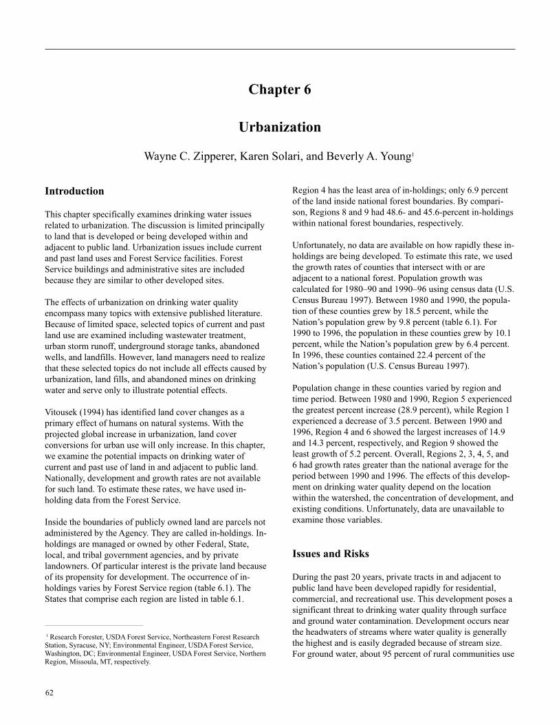
62
Chapter 6
Urbanization
Wayne C. Zipperer, Karen Solari, and Beverly A. Young1
Introduction
This chapter specifically examines drinking water issues
related to urbanization. The discussion is limited principally
to land that is developed or being developed within and
adjacent to public land. Urbanization issues include current
and past land uses and Forest Service facilities. Forest
Service buildings and administrative sites are included
because they are similar to other developed sites.
The effects of urbanization on drinking water quality
encompass many topics with extensive published literature.
Because of limited space, selected topics of current and past
land use are examined including wastewater treatment,
urban storm runoff, underground storage tanks, abandoned
wells, and landfills. However, land managers need to realize
that these selected topics do not include all effects caused by
urbanization, land fills, and abandoned mines on drinking
water and serve only to illustrate potential effects.
Vitousek (1994) has identified land cover changes as a
primary effect of humans on natural systems. With the
projected global increase in urbanization, land cover
conversions for urban use will only increase. In this chapter,
we examine the potential impacts on drinking water of
current and past use of land in and adjacent to public land.
Nationally, development and growth rates are not available
for such land. To estimate these rates, we have used in-
holding data from the Forest Service.
Inside the boundaries of publicly owned land are parcels not
administered by the Agency. They are called in-holdings. In-
holdings are managed or owned by other Federal, State,
local, and tribal government agencies, and by private
landowners. Of particular interest is the private land because
of its propensity for development. The occurrence of in-
holdings varies by Forest Service region (table 6.1). The
States that comprise each region are listed in table 6.1.
Region 4 has the least area of in-holdings; only 6.9 percent
of the land inside national forest boundaries. By compari-
son, Regions 8 and 9 had 48.6- and 45.6-percent in-holdings
within national forest boundaries, respectively.
Unfortunately, no data are available on how rapidly these in-
holdings are being developed. To estimate this rate, we used
the growth rates of counties that intersect with or are
adjacent to a national forest. Population growth was
calculated for 1980–90 and 1990–96 using census data (U.S.
Census Bureau 1997). Between 1980 and 1990, the popula-
tion of these counties grew by 18.5 percent, while the
Nation’s population grew by 9.8 percent (table 6.1). For
1990 to 1996, the population in these counties grew by 10.1
percent, while the Nation’s population grew by 6.4 percent.
In 1996, these counties contained 22.4 percent of the
Nation’s population (U.S. Census Bureau 1997).
Population change in these counties varied by region and
time period. Between 1980 and 1990, Region 5 experienced
the greatest percent increase (28.9 percent), while Region 1
experienced a decrease of 3.5 percent. Between 1990 and
1996, Region 4 and 6 showed the largest increases of 14.9
and 14.3 percent, respectively, and Region 9 showed the
least growth of 5.2 percent. Overall, Regions 2, 3, 4, 5, and
6 had growth rates greater than the national average for the
period between 1990 and 1996. The effects of this develop-
ment on drinking water quality depend on the location
within the watershed, the concentration of development, and
existing conditions. Unfortunately, data are unavailable to
examine those variables.
Issues and Risks
During the past 20 years, private tracts in and adjacent to
public land have been developed rapidly for residential,
commercial, and recreational use. This development poses a
significant threat to drinking water quality through surface
and ground water contamination. Development occurs near
the headwaters of streams where water quality is generally
the highest and is easily degraded because of stream size.
For ground water, about 95 percent of rural communities use
1 Research Forester, USDA Forest Service, Northeastern Forest ResearchStation, Syracuse, NY; Environmental Engineer, USDA Forest Service,Washington, DC; Environmental Engineer, USDA Forest Service, NorthernRegion, Missoula, MT, respectively.
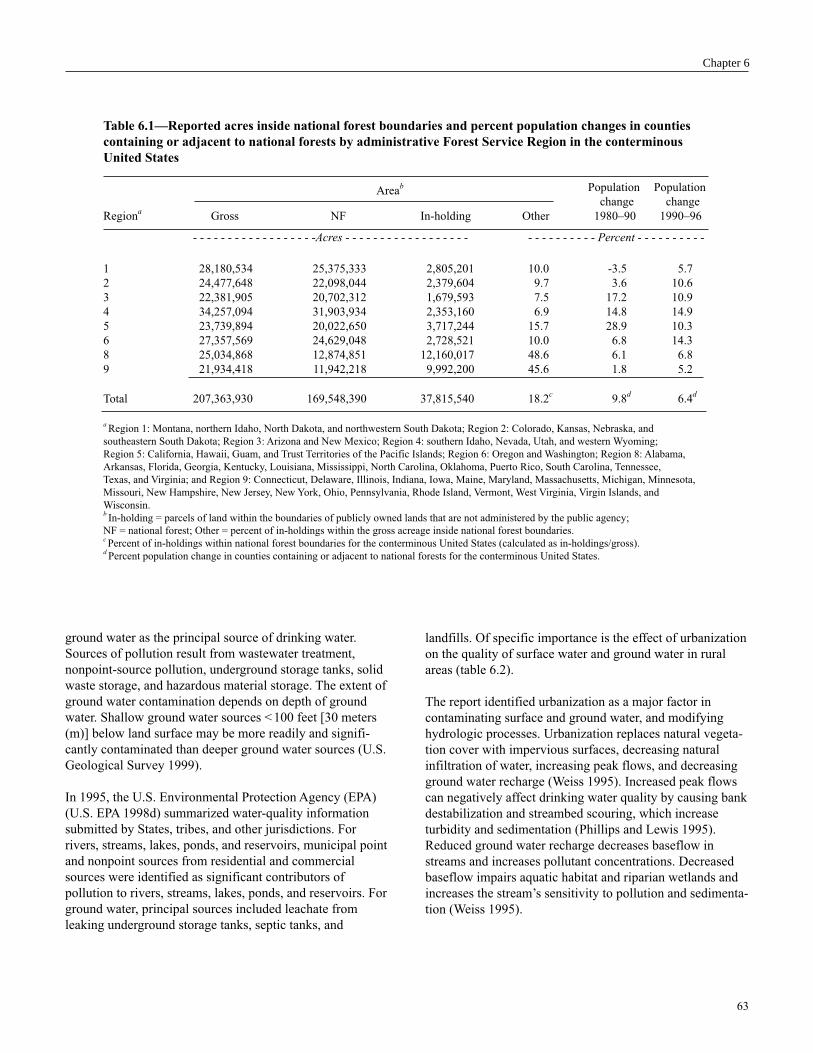
63
ground water as the principal source of drinking water.
Sources of pollution result from wastewater treatment,
nonpoint-source pollution, underground storage tanks, solid
waste storage, and hazardous material storage. The extent of
ground water contamination depends on depth of ground
water. Shallow ground water sources < 100 feet [30 meters
(m)] below land surface may be more readily and signifi-
cantly contaminated than deeper ground water sources (U.S.
Geological Survey 1999).
In 1995, the U.S. Environmental Protection Agency (EPA)
(U.S. EPA 1998d) summarized water-quality information
submitted by States, tribes, and other jurisdictions. For
rivers, streams, lakes, ponds, and reservoirs, municipal point
and nonpoint sources from residential and commercial
sources were identified as significant contributors of
pollution to rivers, streams, lakes, ponds, and reservoirs. For
ground water, principal sources included leachate from
leaking underground storage tanks, septic tanks, and
landfills. Of specific importance is the effect of urbanization
on the quality of surface water and ground water in rural
areas (table 6.2).
The report identified urbanization as a major factor in
contaminating surface and ground water, and modifying
hydrologic processes. Urbanization replaces natural vegeta-
tion cover with impervious surfaces, decreasing natural
infiltration of water, increasing peak flows, and decreasing
ground water recharge (Weiss 1995). Increased peak flows
can negatively affect drinking water quality by causing bank
destabilization and streambed scouring, which increase
turbidity and sedimentation (Phillips and Lewis 1995).
Reduced ground water recharge decreases baseflow in
streams and increases pollutant concentrations. Decreased
baseflow impairs aquatic habitat and riparian wetlands and
increases the stream’s sensitivity to pollution and sedimenta-
tion (Weiss 1995).
Table 6.1—Reported acres inside national forest boundaries and percent population changes in counties
containing or adjacent to national forests by administrative Forest Service Region in the conterminous
United States
Population Population
change change
Regiona
Gross NF In-holding Other 1980–90 1990–96
- - - - - - - - - - - - - - - - - -Acres - - - - - - - - - - - - - - - - - - - - - - - - - - - - Percent - - - - - - - - - -
1 28,180,534 25,375,333 2,805,201 10.0 -3.5 5.7
2 24,477,648 22,098,044 2,379,604 9.7 3.6 10.6
3 22,381,905 20,702,312 1,679,593 7.5 17.2 10.9
4 34,257,094 31,903,934 2,353,160 6.9 14.8 14.9
5 23,739,894 20,022,650 3,717,244 15.7 28.9 10.3
6 27,357,569 24,629,048 2,728,521 10.0 6.8 14.3
8 25,034,868 12,874,851 12,160,017 48.6 6.1 6.8
9 21,934,418 11,942,218 9,992,200 45.6 1.8 5.2
Total 207,363,930 169,548,390 37,815,540 18.2c
9.8d
6.4d
a Region 1: Montana, northern Idaho, North Dakota, and northwestern South Dakota; Region 2: Colorado, Kansas, Nebraska, and
southeastern South Dakota; Region 3: Arizona and New Mexico; Region 4: southern Idaho, Nevada, Utah, and western Wyoming;
Region 5: California, Hawaii, Guam, and Trust Territories of the Pacific Islands; Region 6: Oregon and Washington; Region 8: Alabama,
Arkansas, Florida, Georgia, Kentucky, Louisiana, Mississippi, North Carolina, Oklahoma, Puerto Rico, South Carolina, Tennessee,
Texas, and Virginia; and Region 9: Connecticut, Delaware, Illinois, Indiana, Iowa, Maine, Maryland, Massachusetts, Michigan, Minnesota,
Missouri, New Hampshire, New Jersey, New York, Ohio, Pennsylvania, Rhode Island, Vermont, West Virginia, Virgin Islands, and
Wisconsin.b In-holding = parcels of land within the boundaries of publicly owned lands that are not administered by the public agency;
NF = national forest; Other = percent of in-holdings within the gross acreage inside national forest boundaries.c Percent of in-holdings within national forest boundaries for the conterminous United States (calculated as in-holdings/gross).
d Percent population change in counties containing or adjacent to national forests for the conterminous United States.
Chapter 6
Areab
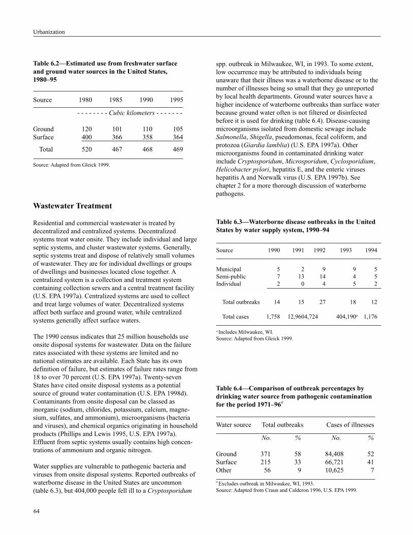
64
Wastewater Treatment
Residential and commercial wastewater is treated by
decentralized and centralized systems. Decentralized
systems treat water onsite. They include individual and large
septic systems, and cluster wastewater systems. Generally,
septic systems treat and dispose of relatively small volumes
of wastewater. They are for individual dwellings or groups
of dwellings and businesses located close together. A
centralized system is a collection and treatment system
containing collection sewers and a central treatment facility
(U.S. EPA 1997a). Centralized systems are used to collect
and treat large volumes of water. Decentralized systems
affect both surface and ground water, while centralized
systems generally affect surface waters.
The 1990 census indicates that 25 million households use
onsite disposal systems for wastewater. Data on the failure
rates associated with these systems are limited and no
national estimates are available. Each State has its own
definition of failure, but estimates of failure rates range from
18 to over 70 percent (U.S. EPA 1997a). Twenty-seven
States have cited onsite disposal systems as a potential
source of ground water contamination (U.S. EPA 1998d).
Contaminants from onsite disposal can be classed as
inorganic (sodium, chlorides, potassium, calcium, magne-
sium, sulfates, and ammonium), microorganisms (bacteria
and viruses), and chemical organics originating in household
products (Phillips and Lewis 1995, U.S. EPA 1997a).
Effluent from septic systems usually contains high concen-
trations of ammonium and organic nitrogen.
Water supplies are vulnerable to pathogenic bacteria and
viruses from onsite disposal systems. Reported outbreaks of
waterborne disease in the United States are uncommon
(table 6.3), but 404,000 people fell ill to a Cryptosporidum
spp. outbreak in Milwaukee, WI, in 1993. To some extent,
low occurrence may be attributed to individuals being
unaware that their illness was a waterborne disease or to the
number of illnesses being so small that they go unreported
by local health departments. Ground water sources have a
higher incidence of waterborne outbreaks than surface water
because ground water often is not filtered or disinfected
before it is used for drinking (table 6.4). Disease-causing
microorganisms isolated from domestic sewage include
Salmonella, Shigella, pseudomonas, fecal coliform, and
protozoa (Giardia lamblia) (U.S. EPA 1997a). Other
microorganisms found in contaminated drinking water
include Cryptosporidum, Microsporidum, Cyclosporidium,
Helicobacter pylori, hepatitis E, and the enteric viruses
hepatitis A and Norwalk virus (U.S. EPA 1997b). See
chapter 2 for a more thorough discussion of waterborne
pathogens.
Table 6.2—Estimated use from freshwater surface
and ground water sources in the United States,
1980–95
Source 1980 1985 1990 1995
- - - - - - - - Cubic kilometers - - - - - - -
Ground 120 101 110 105
Surface 400 366 358 364
Total 520 467 468 469
Source: Adapted from Gleick 1999.
Urbanization
Table 6.4—Comparison of outbreak percentages by
drinking water source from pathogenic contamination
for the period 1971–96a
Water source Total outbreaks Cases of illnesses
No. % No. %
Ground 371 58 84,408 52
Surface 215 33 66,721 41
Other 56 9 10,625 7
a Excludes outbreak in Milwaukee, WI, 1993.
Source: Adapted from Craun and Calderon 1996, U.S. EPA 1999.
Table 6.3—Waterborne disease outbreaks in the United
States by water supply system, 1990–94
Source 1990 1991 1992 1993 1994
Municipal 5 2 9 9 5
Semi-public 7 13 14 4 5
Individual 2 0 4 5 2
Total outbreaks 14 15 27 18 12
Total cases 1,758 12,9604,724 404,190a 1,176
a Includes Milwaukee, WI.
Source: Adapted from Gleick 1999.

65
The fate and transport of parasites, bacteria and viruses from
sewage effluent depend on the characteristics of the subsur-
face environment (U.S. EPA 1997a). Pore size and chemical
charges of the soil matrix are important in removing bacteria
and viruses. Bacteria have been reported to travel distances
of up to 300 feet (100 m) in sand aquifers, 2,500 feet (800
m) in gravel aquifers, and over 3,000 feet (1000 m) in
limestone rock (Kaplan 1991). Certain viruses, because of
their size and long survival times, can travel distances up to
1 mile [1.6 kilometers (km)] in areas with karst geology
(Yates and Yates 1989).
Organic chemicals in onsite disposal systems are a less
commonly reported problem because they often are below
levels considered hazardous to human health (U.S. EPA
1997a). These chemicals can significantly affect aquatic
systems, however. Organic chemicals commonly found in
septic systems originate from household products, paints
and varnishes, shampoos, cosmetics, and polishes.
Septic systems fail for two reasons: poor design or poor
maintenance (Kelley and Phillips 1995). Design includes
construction, soils and hydrological characteristics of the
site, and drainfield layout (Kelley and Phillips 1995). If
drainage is too slow, there will be upward seepage and
ponding, which are likely to contaminate surface water. If
drainage is too fast, downward percolation occurs without
sufficient biological treatment; contamination of ground
water is likely to result.
Even with properly installed systems, maintenance is
absolutely necessary. Unfortunately, the typical owner of an
onsite disposal system is unaware of the need for proper
maintenance (Kelley and Phillips 1995). Maintenance
includes periodic testing of drainfields and emptying of
septic tanks. Frequency of maintenance depends on soil
conditions, type of septic system, and weather patterns.
Class V injection wells is another type of onsite disposal
unit. An injection well can include any manmade hole in the
ground for injection of wastewater (U.S. EPA 1998a). They
are used by dry cleaners, laundromats, paint dealers,
hardware stores, funeral homes, and other industrial and
commercial facilities for materials other than domestic and
sanitary wastes. Motor vehicle waste disposal wells,
industrial waste disposal wells, and large-capacity cesspools
have high risk for ground water contamination. Field studies
have shown that ground water sources can be degraded
significantly by organic and inorganic contaminants from
dry wells in automotive shops (Ogden and others 1991).
See the section on abandoned wells in this chapter.
Approximately 10 percent of the wastewater produced
in the United States originates from communities of
< 10,000 people. With the passage of the Clean Water Act in
1972, many such communities elected to use Federal funds
to install centralized systems for wastewater treatment. In
small communities, contractors frequently installed the most
economical and not necessarily the most effective systems.
Currently, many of these systems are obsolete and need
replacing because they have operated beyond their 20–year
life span. Small communities also face an economic factor
of scale. Costs of maintenance and staffing must be divided
among fewer people, resulting in higher costs per person.
Consequently, small communities have nearly twice the
number of violations than larger communities (> 10,000
individuals). Violations include leaking sewage systems
(cracked and broken sewer lines), illegal connections of
sewer and storm drainage lines, and inadequate treatment.
Violations often affect local water quality and potentially
affect drinking water quality for downstream communities.
Since 1970, new technologies have been developed to treat
water more effectively and cheaply. However, many small
communities have not adopted these systems because of a
lack of knowledge, public distrust of new technologies, and
legislative and regulatory constraints (U.S. EPA 1994).
Additional discussion of centralized wastewater treatment
can be found in chapter 5.
Urban Runoff
Findings
Urban land generates nonpoint-source pollution. People
apply various chemicals around their homes, businesses, and
adjacent land. These chemicals are carried by surface runoff
to receiving waters. As land is developed and impervious
surface area increases, the amount of urban runoff increases.
Consequently, land development increases the amount of
nonpoint-source pollutants discharged into surface water
(Phillips and Lewis 1995). The Nationwide Urban Runoff
Program (U.S. EPA 1983) reported that 10 times as much
suspended solid material was being discharged from storm
sewers serving residential and commercial areas as was
discharged from sewage treatment plants providing second-
ary treatment (Weiss 1995). Major pollutants associated
with residential and commercial runoff include floatables,
sediments, suspended solids, oxygen-demanding materials,
nutrients, organics, biocides (herbicides, fungicides,
pesticides), polycyclic aromatic hydrocarbons, and petro-
leum hydrocarbons (U.S. EPA 1997a, Weiss 1995).
Because residential and commercial construction creates site
disturbances, it is highlighted here. Sediment loading from
site preparation, and construction and maintenance of
buildings and roads can exceed the capacity of streams to
Chapter 6
66
transport it (Yoder 1995). Sediment loads from inadequately
controlled construction sites typically are 10 to 20 times per
unit of land area those from agricultural land and 1,000 to
2,000 times those from forest (Weiss 1995). In a relatively
short period, urban site construction can contribute more
sediment to a stream than was deposited over the previous
several decades (Weiss 1995).
Urban runoff is highly intermittent. Short-term loading,
associated with individual storms, is high and may have a
shock effect on the receiving water (Weiss 1995). When
predicting the effect of urban runoff on water quality, it is
important to determine the duration of the effect. Effects
may be acute (short term) or chronic (long term) (Phillips
and Lewis 1995). Oxygen-demanding substances and
bacteria create acute effects; whereas nutrients, sediments,
toxic metals, and organics create chronic effects. For an
acute effect, estimates are based on the probability that
pollution concentrations will exceed acceptable drinking
water standards (Phillips and Lewis 1995). For a chronic
effect, a simple method has been developed to predict the
increase in pollution loading above current conditions (U.S.
EPA 1983). This simple method is employed by EPA and
uses information readily available to the resource manager.
Input variables include pollutant type and concentration,
precipitation, and percent impervious cover. The method,
however, is limited to areas < 1 square mile (2.6 km2).
Findings from engineering research show that pollution and
sediment loading from runoff can be reduced. Practices for
mitigating storm runoff include attenuation, conveyance,
pretreatment, and treatment of runoff (U.S. EPA 1997a).
When selecting mitigation practices, it is important to
consider
• How will practices meet watershed and site objectives?
• What are the limitations of a practice to meet objectives?
• What are the drainage field, soil types, and topography?
• Are practices compatible with a region’s rainfall pattern
and annual runoff?
• Are they derived from scientific research?
• How will practices function as a system (Phillips and
Lewis 1995)?
A number of manuals and practical guides have been written
to select, design, and maintain mitigation practices to meet
local, State, and Federal mandates (Birch 1995, Phillips and
Lewis 1995). As with plans and guides for wastewater
treatment, managers need to check with State and local
agencies for specific performance ratings and regulations.
Like wastewater treatment facilities, new mitigation
practices must be maintained and existing ones upgraded to
meet expected performance standards. Adequate funds often
are lacking to maintain or enhance these facilities (U.S. EPA
1997a). Without proper maintenance, water quality degrades
as systems fail.
Reliability and Limitation of Findings
Although development of private land in or adjacent to
public land has occurred for decades, scientific studies of
the effects on water quality and drinking water sources are
lacking. Extensive research has been conducted on urban
effects on natural systems, however. These studies provide
the basis for identifying the potential impacts of develop-
ment on drinking water.
When applying findings across a watershed, scale becomes
an important issue. Evaluating cumulative effects requires
examination of more than just local impacts of individual
pollution sources, such as urban runoff, wastewater treat-
ment, and landfills. The timing and location of all activities
that contribute contaminants within the watershed and their
hydrologic connection to source water intakes must be
considered to estimate cumulative effects. Consequently,
these developments must be evaluated both independently
and collectively within the watershed. Ages of wastewater
treatment facilities and urban storm runoff structures must
be considered. For various reasons, existing infrastructures
may not meet sanitation and water-quality regulations.
Success of management plans to mitigate the effects of
wastewater treatment and urban runoff is predicated on
sound infrastructure.
The ability to address the effects of development on
drinking water quality depends on ownership. On publicly
owned land, resource managers directly determine whether
facilities comply with Federal and State regulations. On
privately owned land, resource managers can only indirectly
influence development effects on drinking water quality
through the planning process.
Planning and development of private land in and adjacent to
public land involve complex issues including the interplay
of the physical, biological, and social components of a
watershed. A number of factors need to be considered. First,
planning must include all stakeholders, including public
land managers. Second, private tracts are owned by a
diversity of individuals for various reasons. Third, new
regulations often cause resentment among landowners.
Any changes in drinking water regulations and statutes
create the need for communication and education. Fourth,
a comprehensive approach is needed to account for the
Urbanization

67
cumulative effects of individual developments in a water-
shed and to address the needs of individual stakeholders.
Because of the interplay, technology and management
practices are not the only solutions to drinking water issues.
A number of communities have adopted a whole watershed
approach to manage water and land planning issues (Birch
1995, Kelley and Phillips 1995, Phillips and Lewis 1995).
This approach provides a framework not only to design the
optimal mix of water-quality management strategies but also
to design land management strategies by integrating and
coordinating management priorities across stakeholders,
governments, and agencies. Livingston (1993) identifies
the big “C’s” of watershed management that must be
considered:
• Comprehensive management.
• Continuity of management over a long period.
• Cooperation among Federal, State, local, and tribal
governments; cities and counties; public and private
sectors; and all citizens.
• Communication to educate elected officials and ourselves.
• Creativity in best-management-practice technology.
• Coordination of stormwater retrofitting to reduce pollu-
tion loading.
• Consistency in implementing laws, rules, and programs.
• Commitment to solving current problems and preventing
future ones.
• Cash in funding programs and maintenance over a long
period.
Research Needs
Development of private tracts in and adjacent to public land
represents an opportunity to examine how development
alters ecosystem processes and what are the long-term
implications of these changes.
1. Long-term monitoring stations are needed not only to
monitor changes in water quality and habitat modification
but also atmospheric deposition.
2. In addition, studies are needed to determine the limitation
of management practices, wastewater treatment, and
urban runoff in extreme environments such as at high
elevations [> 8,000 feet (> 2,400 m)]. Research also is
needed to determine threshold levels of the corresponding
changes in processes that affect source water quality as
land use shifts to urban.
Key Points
1. Levels of drinking water protection need to increase with
increasing amounts of urban development.
2. Because of their depth, shallow ground water sources are
especially prone to contamination from septic systems.
3. Septic systems fail for two reasons: poor design and poor
maintenance.
4. Septic system designs need to consider site conditions,
such as soil characteristics (permeability, depth to
bedrock, depth to ground water table), topography
(floodplain, hillslope, ridge top), and climatic patterns
(rainfall and snowfall amounts and patterns, winter
temperatures).
5. A comprehensive approach towards development
planning must be taken. The approach needs to consider
issues ranging from the local to watershed scale.
6. Urban runoff is reduced by maintaining and enhancing
existing vegetation and by minimizing the amount of
impervious surfaces.
Underground Storage Tanks
Issues and Risks
Underground storage tanks pose a risk of ground water
contamination because nearly all tanks contain petroleum
products. The tanks are associated with service stations,
convenience stores, and organizations that have fleets of
vehicles (U.S. EPA 1998b). Current estimates indicate that
25 to 35 percent of these tanks do not comply with existing
regulations. In 1986, EPA published regulations with the
goals of preventing and cleaning up releases from under-
ground storage tanks. These regulations (40 CFR 280)
require that underground storage tanks, which contain
hazardous substances, including fuels, be removed by
December 1998 or have spill, overfill, and corrosion
protection. The regulations also require that installation and
closure of underground storage tanks must be registered
with the State or EPA. These regulations have had a signifi-
cant impact on land management agencies, which, due to the
remote locations of administrative offices, recreation sites,
and workshops, have installed underground storage tanks for
easy access to fuel. For example, in order to comply with
these regulations, the Forest Service has removed over 1,600
underground storage tanks and has initiated several projects
to cleanup contaminated soil caused by leaking tanks.
Chapter 6

68
The primary concern about underground storage tanks is
leakage, which can seep into the soil and contaminate
ground water. Since 1988, over 330,000 confirmed releases
have occurred from regulated underground storage tanks.
Gasoline is the most common contaminate of ground water.
Although not all of those releases contaminated ground
water, drinking water wells have been shut down because of
petroleum contamination (U.S. EPA 1996). In 1988, EPA
regulations established minimum standards for new tanks
and required owners to upgrade existing tanks, to replace
them, or close them by December 1998 (U.S. EPA 1996).
Findings
Recent studies have identified methyl tertiary butyl ester
(MTBE) as a potential major health hazard in drinking
water. Methyl tertiary butyl ester is added to gasoline to
increase its oxygen content and to reduce airborne emis-
sions. Effects on drinking water include widespread impacts
from low concentrations and local impacts from high
concentrations (U.S. EPA 1998c) (see chapter 7 for more
detailed information on the effect of vehicular emissions).
Local impacts primarily result from leaking underground
storage tanks. A survey of ground water plume data from
over 700 service stations showed that 43 percent of the sites
had MTBE concentrations > 1,000 micrograms (µg) per
liter. However, a survey of drinking water wells from 20
National Water Quality Assessment study units showed that
2 percent of 949 rural wells had a median concentration of
approximately 0.5 µg per liter (well below the EPA drinking
water advisory of 20 to 24 µg per liter) (U.S. EPA 1998c,
Zogorski and others 1998). A study of private wells in
Maine showed 1.1 percent of 951 wells with MTBE levels
exceeding 35 µg per liter. Maine officials estimated that
1,400 to 5,200 private wells across the State could be
contaminated at levels exceeding 35 µg per liter (U.S. EPA
1998c). The potential threat of underground storage tanks
contaminating ground water should diminish as older tanks
are upgraded and sites are cleared of contaminates.
Reliability and Limitation of Findings
Records should be available through the State or EPA
identifying where underground storage tanks are located,
where cleanup operations are ongoing, and where tanks
have been removed. The possibility also exists that under-
ground storage tanks may be present and not registered with
the appropriate agency. During field visits, resource manag-
ers need to look for indications of former structures or
operations on the property, and they need to note the
presence of partially exposed, capped, or uncapped pipes.
These pipes may be vent pipes or fill pipes for underground
storage tanks. On properties where motor vehicles were
operated regularly, be skeptical where there is no apparent
refueling source. An underground storage tank is likely to be
present (U.S. Department of Agriculture, Forest Service
1999).
Research Needs
1. More data are needed to determine the extent of contami-
nation of drinking water sources by MTBE and the
potential health hazard.
2. Research also is needed to develop more effective and
cost efficient cleanup methods. Cleanup of ground water
and soil contaminated by leaking underground storage
tanks can be expensive and take long periods of time.
Key Points
Underground storage tanks are a potential threat to drinking
water supplies through contamination of surface and ground
water by storage tanks that have leaked or have been
overfilled.
Abandoned Wells
Issues and Risks
Abandoned wells and wells that are no longer used may or
may not have been properly closed or plugged after their use
ceased. Abandoned wells are of concern because they can
serve as conduits for migration of contaminants into aquifers
and between aquifers.
Numerous types of abandoned wells exist on public land.
Some were drilled for mineral exploration, others for oil and
gas production, and still others for stock watering. Those
associated with administrative and recreational develop-
ments include water wells for irrigation and drinking water
and disposal wells for stormwater runoff or waste products
from vehicle shops. Septic systems may be considered
disposal wells when industrial or commercial wastes are
treated along with sanitary wastes.
Although Federal, State, and local regulations address
proper closure of abandoned wells, not all abandoned wells
have been closed or plugged properly. Many of the improp-
erly closed wells were abandoned before regulations existed.
Other wells have been abandoned temporarily to allow for
further use if the need should arise. Certain wells, such as
automotive dry wells in vehicle shops, may still be in use
but would be banned or subject to permit under proposed
Urbanization

69
regulations for Underground Injection Control (U.S. EPA
1998e). Certain States already have banned such dry wells
and have required cleanup, per the Resource Conservation
and Recovery Act of 1976, due to contamination at such
sites.
The number of abandoned wells on public land is unknown.
For example, the Forest Service has inventories of some
categories of in-use wells but not of abandoned wells.
Knowledge of number and location of such wells is limited,
and in most instances, might be gained only by a field
survey.
Findings
Abandoned wells are commonly cited as avenues of
contamination in Federal, State, and local programs dealing
with ground water protection (Nye 1987). The EPA’s Adopt
Your Watershed campaign supports properly closing
abandoned wells. Many States, such as Iowa, Kansas, and
Nebraska, provide financial incentives for proper well
abandonment because it is considered so important for
ground water protection.
Proper abandonment of water wells is regulated at the State
or local level. Oil and gas well closure is specified in 43
CFR 3160. Motor vehicle waste disposal wells (dry wells)
are regulated in the underground injection control program
as class V wells (40 CFR 146).
Field studies have shown that ground water sources can be
degraded significantly by organic and inorganic contami-
nants from stormwater runoff and dry wells in automotive
shops (Ogden and others 1991). In certain geologic forma-
tions, abandoned water wells are prone to collapse, and,
when wells are drilled through multiple aquifers, contamina-
tion problems may occur (Blomquist 1984). Gass (1988)
reported that abandoned water supply wells became con-
duits for cross contamination between aquifers. Abandoned
oil and gas wells allowed leakage of contaminated or highly
mineralized water, leading to ground water pollution
including salinization (Gass 1988). Even plugged boreholes
may have defects in structural integrity, allowing pollutant
transport between confined aquifers (Avci 1992).
Reliability and Limitation of Findings
The issue of abandoned well closure is well defined in
Federal, State, and local regulations. The extent of the
problem on public land is unknown because wells have not
been inventoried. Proper well closure is heavily regulated at
present, but not heavily enforced. Existence of improperly
closed wells does not mean ground water contamination will
occur; only that it is has the potential to occur.
Wells on public land possess the same general characteris-
tics as other abandoned wells. Drilling and development
methods for all types of wells have usually followed
industry standards. For all types of wells, the newer the well
the more likely that it was drilled and closed properly. On
public land, dry wells in vehicle shops may not have as
much waste or as much variety of waste in them as a
commercial facility would, but the pollution potential still
exists. Some could have greater potential for contamination
than others because of hydrogeologic formations and
duration of well use. For example, in the Allegheny and
Appalachian Mountains, where abandoned oil and gas wells
are more numerous and older, problems may be greater than
in other regions of the country.
Research Needs
1. Methods need to be developed to inventory abandoned
wells on both public and private land. Inventorying
methods need to incorporate the capabilities of remote
sensing technology and Geographical Information
Systems.
2. The inventorying process also needs to be linked to a
monitoring program.
3. Further, an abandoned-well typology needs to be
developed that integrates type of well, geological
formation, soil, typography, climate, and potential for
ground water contamination.
Key Points
1. Abandoned wells may serve as conduits for the transport
of pollutants.
2. Where there may be no records of abandoned wells on a
property, the property must be surveyed to locate wells.
3. The type of abandoned well influences the types of
pollution that may enter ground water sources.
4. Improperly sealed abandoned wells may be a source of
contamination.
Chapter 6

70
Solid Waste Landfills and Other
Past Land Uses
In 1990, citizens in the United States generated over 195
million tons [215 million metric tonnes (Mg)] of municipal
solid waste. Currently, over 6,000 regulated municipal
landfills exist (U.S. EPA 1993). However, an estimated
30,000 to 50,000 unregulated waste disposal sites are
thought to exist in the United States (Woldt and others
1998). Both regulated and unregulated sites may have
impacts on water quality and the environment. In 1976, the
Resource Conservation and Recovery Act (RCRA) ad-
dressed waste management and separated hazardous waste
management from solid waste management. Prior to RCRA,
municipal and industrial wastes were deposited at the same
landfills. The practice was to spread hazardous waste sludge
and liquids over municipal waste, using the municipal waste
to soak up the sludge (Brown and Donnelly 1988). Conse-
quently, landfills existing prior to RCRA may contain
hazardous waste and may be the origin of organic com-
pounds found in municipal landfill leachate. Other sources
of hazardous materials in landfills include household and
agricultural materials, incinerator ash, and sewage sludge.
The U.S. EPA (1993) defines a municipal solid waste
landfill as:
A discrete area of land or an excavation that receives
household waste, and that is not a land application
unit, surface impoundment, injection well, or waste
pile, as those terms are defined in the law. (House-
hold waste includes any solid waste including
garbage, trash, and septic waste derived from houses,
apartments, hotels, motels, campgrounds, and picnic
grounds.) A municipal solid waste landfill unit also
may receive other types of waste such as commercial
solid waste, non-hazardous sludge, small quantities of
generator waste, and industrial solid waste.
In many rural areas, small communities are served by small
landfills that may be exempt from some regulatory require-
ments. The U.S. EPA (1993) defines a small landfill as one
that receives less than an average of 20 tons (22 Mg) of
waste per day, receives < 25 inches (62.5 centimeters) of
rain per year, and shows no evidence of ground water
contamination. About half of the regulated landfills serve
communities with < 10,000 people and are considered small
landfills. Many of these small landfills may be on or
adjacent to public land.
Issues and Risks
Municipal solid waste landfills that contaminated ground
water often were poorly designed, located in geologically
unsound areas, or accepted toxic materials without proper
safeguards (U.S. EPA 1993). Decomposing municipal solid
waste in landfills form leachates, liquids containing ex-
tremely high concentrations of organic and inorganic
pollutants. Ground water contamination is common near
landfills, but the effect may decrease with distance (Borden
and Yanoschak 1990). A study of 71 North Carolina sanitary
landfills found that 53 percent had ground water violations
for organic and inorganic pollution based on North Carolina
ground water-quality standards (Borden and Yanoschak
1990). Only a few landfills had organic contamination.
When predicting the performance of a landfill, it is impor-
tant to know its age, history of material disposal, design, and
capability of handling toxic waste.
Another threat of landfills to ground water is volatile
organic compounds (VOC). Volatile organic compounds
come from biological and chemical degradation of materials
in the landfill. Recently, VOC’s have been detected in
ground water (Baker 1998) and management procedures
have been developed to minimize this threat (Rickabaugh
and Kinman 1993). Ground water contamination was linked
to methane diffusion as VOC concentrations increased.
Mitigation involves improving gas removal systems at the
landfill (Baker 1998). The extent of ground water contami-
nation by VOC’s and subsequent health effects need to be
evaluated further.
Illegal dumping may occur on or adjacent to public lands.
This practice is usually done to avoid disposal fees or the
time and effort required for proper disposal. Dumped
materials may include nonhazardous material such as scrap
tires, yard waste, and construction waste. It also may include
hazardous waste such as asbestos, household chemicals and
paints, automotive fluids, and commercial or industrial
waste. The potential for contaminated runoff and ground
water depend on such factors as the proximity of the dump
to surface water, elevation of the ground water table, and
permeability of the soil.
Other sources of contamination on public land include
shooting ranges, formerly used defense sites, and wood
treatment sites. Shooting ranges pose the potential for lead
contaminates entering surface water and ground water.
Acidic rainfall or acidic soil can dissolve the weathered lead
compounds. In a dissolved state, lead can move through the
soil and enter surface water and ground water. Shooting
ranges in areas with acidic soils or acidic rainfall have an
increased potential for transporting contaminates offsite and
into drinking water. Bare ground on ranges may further
increase the risk of migration of lead compounds offsite.
Sites once used by the Department of Defense (DOD) for
military training and industrial facilities are on both public
Urbanization

71
and private land. The DOD estimates that over 9,000 such
sites exist. They pose a wide range of environmental
hazards, including unexploded ordinances from the training
sites and soil contamination from solvents, fuels, and other
petroleum compounds used at industrial facilities. Sites are
being cleaned up to minimize environmental effects. The
Forest Service, for example, has identified over 100
formerly used defense sites on national forests.
Field treatment of wood posts is another past land-use
activity that may have led to surface and ground water
contamination. The common practice was to dip wooden
posts into tanks that contained creosote, pentachlorophenol,
or a chromium, copper, and arsenic compound and move
them to an area for dripping and drying. The practice has
been discontinued on public land such as national forests.
However, a potential exists for surface and ground water
contamination from past wood treatment operations.
Reliability and Limitation of Findings
Most available information on types of hazardous material
activities and the contaminants associated with these
activities is reliable because it is based on extensive site-
specific data from Federal agency hazardous waste site
cleanup programs. A limitation is that inventories identify-
ing all hazardous waste sites on or adjacent to public land
are incomplete. During field visits, areas of stressed
vegetation, discolored or stained soil and water, indications
of former structures or operations, and land disturbances
may indicate the presence of old, abandoned, or illegal
waste disposal sites. Due to the potentially hazardous nature
of these disposal sites, discovery of such conditions should
be reported to the appropriate agency official for further
action (U.S. Department of Agriculture, Forest Service
1999). Other potential sources of ground water and surface
water contamination, which should be considered in
conducting source water assessments, are cemeteries and
small airports and airstrips, especially those used for aerial
application of chemicals.
Because the need for landfills exists, the design and man-
agement of safe landfills are paramount. To meet this need,
Federal, State, tribal, and local governments have adapted
an integrative approach that involves three waste manage-
ment techniques: (1) decreasing the amount of waste
through source reduction, (2) recycling of materials, and
(3) improving design and management of landfills (U.S.
EPA 1993). A number of regulations exist for the manage-
ment of a municipal solid waste landfill, and many regula-
tions have flexibility to meet local conditions; managers are
advised to contact a local EPA or State agency office for
information on siting, designing, and managing for their
landfill.
Research Needs
Cleanup of ground water and soil contaminated by solid and
hazardous wastes can be expensive and take long periods of
time. Research is needed to develop more effective and
cheaper cleanup methods.
Key Points
Several factors need to be considered when resource
managers address the effects of landfills on drinking water
quality:
1. Identification of landfill sites—proximity to wells,
aquifers, geological and hydrological features, and
surface waters.
2. Knowledge of the landfill age (a) old landfills—landfills
existing before RCRA may contain hazardous material
and may be improperly designed for hazardous material
storage and municipal waste; (b) existing landfills—
landfills existing after RCRA may still pose a problem for
ground water contamination because the site may contain
older units where hazardous waste was deposited
improperly (these sites may have been improperly
designed or may have punctured liners or clay layers);
and (c) new landfills—landfills being managed under
current Federal and State regulation should pose fewer
problems, but small landfills may be exempted from
certain regulations.
3. Knowledge of landfill history—What was deposited on the
site and when? How was the landfill constructed? Does it
have a clay layer, a liner, or a combination of the two?
4. Monitoring data—Is the site being monitored for VOC’s
and ground water contamination? Is monitoring sufficient
to safeguard ground water sources?
5. Extent of contamination plume—If ground water is
contaminated, what is the vertical and horizontal extent
of the contamination? What is the effect of the plume on
drinking water sources?
6. Compliance with current Federal and State regulations—
What mitigation actions have been taken to comply with
Federal and State laws if contamination occurred?
Chapter 6

72
Literature Cited
Avci, C.B. 1992. Flow occurrence between confined aquifers through
improperly plugged boreholes. Journal of Hydrology. 139 (1): 97–114.
Baker, J.A. 1998. What’s in your groundwater? Waste Age. 29: 213–224.
Birch, P.B. 1995. New development standards in the Puget Sound Basin.
In: National conference on urban runoff management: enhancing urban
watershed management at the local, county, and State levels. Cincinnati,
OH: U.S. Environmental Protection Agency, Office of Research and
Development, Center for Environmental Research Information: 88–95.
Blomquist, P.K. 1984. Abandoned water wells in southern Minnesota. In:
Proceedings of the 7th national ground water quality symposium:
Innovative means of dealing with potential sources of groundwater
contamination; 1984 September 26–28; Las Vegas, NV. Worthington,
OH: National Water Well Association: 330–342.
Borden, R.C.; Yanoschak, T.M. 1990. Ground and surface water quality
impacts of North Carolina sanitary landfills. Water Resources Bulletin.
26: 269–277.
Brown, K.; Donnelly, K.C. 1988. Estimation of the risk associated with
the organic constituents of hazardous and municipal landfill waste.
Hazardous Waste and Hazardous Materials. 5: 1–30.
Craun, G.F.; Calderon, R. 1996. Microbial risks in groundwater systems,
epidemiology of waterborne outbreaks. In: Under the microscope:
Proceedings of the groundwater foundations’s 12th annual fall sympo-
sium; 1996 September 5–6; Boston. Denver: American Water Works
Association Research Foundation: 9–15.
Gass, T.E. 1988. Impact of abandoned wells. Water Well Journal. 42 (1):
48–49.
Gleick, P.H. 1999. The World’s water 1998–1999. Washington, DC: Island
Press. 307 p.
Kaplan, B.O. 1991. Degradation of groundwater by septic tank systems.
In: Kaplan, B.O., ed. Septic systems handbook. Chelsea, MI: Lewis
Publishers: 133–144.
Kelley, M.; Phillips, N. 1995. Ordinances for the protection of surface
water bodies: septic systems, docks, and other structures, wildlife
corridors, sensitive aquatic habitats, vegetative buffer zones, and bank/
shoreline stabilization. In: National conference on urban runoff
management: enhancing urban watershed management at the local,
county, and State levels; 1993 March 30–April 2; Chicago. Cincinnati:
U.S. Environmental Protection Agency, Center for Environmental
Research Information, Office of Research and Development: 96–109.
Livingston, E.H. 1993. Watershed planning and program integration. In:
National conference on urban runoff management: enhancing urban
watershed management at the local, county, and State levels; 1993
March 30–April 2; Chicago. Cincinnati: U.S. Environmental Protection
Agency, Center for Environmental Research Information, Office of
Research and Development: 1–12.
Nye, J.D. 1987. Abandoned wells: how one State deals with them. Water
Well Journal. 41(9): 42–46.
Ogden, A.E.; Redman, R.K.; Brown, T.L. 1991. Preliminary assessment
of the impact of class V injection wells on karst groundwater. In:
Appalachian karst: Proceedings of the Appalachian karst symposium;
1991 March; Radford, VA. Huntsville, AL: National Speleological
Society, Inc.: 211–216.
Phillips, N.J.; Lewis, E.T. 1995. Site planning from a watershed
perspective. In: National conference on urban runoff management:
enhancing urban watershed management at the local, county, and State
levels; 1993 March 30–April 2; Chicago. Cincinnati: U.S. Environmen-
tal Protection Agency, Office of Research and Development, Center for
Environmental Research Information: 139–150.
Rickabaugh, J.F.; Kinman, R.N. 1993. Evaluation of trace VOC
emissions from sanitary landfills. Journal of Environmental Engineering.
119: 645–657.
U.S. Census Bureau. 1997. Estimates of the population of counties: annual
time series, July 1, 1990, to July 1, 1996 (CO–96–1)(includes revised
April 1, 1990, census population counts). Washington, DC: U.S. Census
Bureau, Population Division, Statistical Information Staff. [Not paged].
[Available on the Web at: http://www.census.gov/population/censusdata/
table-16.pdf and http://www.census.gov/population/projections/state/
yr95to00/].
U.S. Department of Agriculture, Forest Service. 1999. Forest Service
guide to land transactions. EM–2160–2. Washington, DC: U.S.
Department of Agriculture, Forest Service, Engineering Staff. 27 p.
U.S. EPA. 1983. Results of the nationwide urban runoff program. PB84–
185552. Washington, DC: U.S. Environmental Protection Agency. 188 p.
U.S. EPA. 1994. Drinking water treatment for small communities. EPA/
V640/K–94/003. Washington, DC: U.S. Environmental Protection
Agency, Office of Research and Development. 48 p.
U.S. EPA. 1996. UST program facts. EPA–510–B–96–007. Washington,
DC: U.S. Environmental Protection Agency. 18 p.
U.S. EPA. 1997a. Large-capacity septic systems. Draft document EPA–
816–R–97–002. Washington, DC: U.S. Environmental Protection
Agency, Office of Water. 38 p.
U.S. EPA. 1997b. Research plan for microbial pathogens and disinfection
by-products in drinking water. EPA/600/–97/122. Washington, DC: U.S.
Environmental Protection Agency, Office of Research and Development,
Office of Water: 3–1 to 3–52.
U.S. EPA. 1998a. Class V injection wells. EPA/816–F–98–009. Washing-
ton, DC: U.S. Environmental Protection Agency, Office of Water. 4 p.
U.S. EPA. 1998b. Overview of the Federal UST program. Washington, DC:
U.S. Environmental Protection Agency. [Not paged]. [Available on the
Web at: http://www.epa.gov/swerust1/overview.htm].
U.S. EPA. 1998c. Oxygenates in water: critical information and research
needs. EPA/600/R–98/048. Washington, DC: U.S. Environmental
Protection Agency, Office of Research and Development. 65 p.
U.S. EPA. 1998d. The quality of our Nation’s water: 1996. EPA–841–S–
97–001. Washington, DC: U.S. Environmental Protection Agency. 197 p.
U.S. EPA. 1998e. Revisions to the underground injection control
regulations for class V injection wells. Federal Register. 63(145):
40,586–40,619.
Urbanization

73
U.S. EPA. 1999. Ground water rule proposal. Draft document EPA 99–022.
Washington, DC: U.S. Environmental Protection Agency. 78 p.
U.S. Geological Survey. 1999. The quality of our Nation’s water—
nutrients and pesticides: Circ. 1225. Denver: U.S. Geological Survey.
82 p.
Vitousek, P.M. 1994. Beyond global warming: ecology and global change.
Ecology. 75: 1861–1876.
Weiss, K. 1995. Stormwater and the Clean Water Act: municipal separate
storm sewers in the moratorium. In: National conference on urban runoff
management: enhancing urban watershed management at the local,
county, and State levels; 1993 March 30–April 2; Chicago. Cincinnati:
U.S. Environmental Protection Agency, Center for Environmental
Research Information, Office of Research and Development: 47–62.
Woldt, W.E.; Hagemeister, M.E.; Jones, D.D. 1998. Characterization of
an unregulated landfill using surface-based geophysics and geostatistics.
Ground Water. 36: 966–974.
Yates, M.V.; Yates, S.R. 1989. Septic tank setback distances: a way to
minimize virus contamination of drinking water. Ground Water. 27:
202–208.
Yoder, C.O. 1995. Incorporating ecological concepts and biological criteria
in the assessment and management of urban nonpoint source pollution.
In: National conference on urban runoff management: enhancing urban
watershed management at the local, county, and State levels; 1993
March 30–April 2; Chicago. Cincinnati: U.S. Environmental Protection
Agency, Center for Environmental Research Information, Office of
Research and Development: 183–197.
Zogorski, J.S.; Delzer, G.C.; Bender, D.A. [and others]. 1998. MTBE:
summary of findings and research by the U.S. Geological Survey. In:
Proceedings of the 1998 annual conference of the American Water
Works Association—water quality; 1998 June 21–25; Dallas. Denver:
American Water Works Association: 287–309.
Chapter 6

74
Chapter 7
Concentrated Recreation
Myriam Ibarra and Wayne C. Zipperer1
Introduction
This chapter specifically examines drinking water issues
related to concentrated recreation. The effects of concen-
trated recreation on drinking water quality encompass many
topics with limited published literature. Because of limited
space, selected components—campgrounds, ski resorts,
water recreation, and traffic—are discussed in this report.
However, land managers need to realize that these selected
topics do not include all effects caused by concentrated
recreation on drinking water and serve only to illustrate
potential effects.
One of the most important attractions for public recreation
is public land with natural cover. Increased demands for
outdoor recreation result in greater needs for drinking water
and in increased amounts of wastewater. Expanding
recreation resorts invites larger numbers of visitors, and
private tracts adjacent to public land are magnets for real
estate development. This development may negatively affect
drinking water and alter hydrologic processes. To illustrate
the effects of concentrated recreation on drinking water
supplies, we use data from the Forest Service, but our
findings and recommendations are applicable to managers
of other public and private land.
The National Forest System is the single largest supplier of
public outdoor recreation in the United States. The national
forests offer visitors 4,385 miles of national wild and scenic
rivers; one-third of the National Wilderness Area System;
about 8,000 miles of scenic byways; 133,000 miles of trails;
more than 18,000 campgrounds, picnic areas, and visitor
facilities; and 2.3 million acres of fishing lakes, ponds, and
reservoirs. The Forest Service manages over 23,000
developed facilities, including campgrounds, trailheads, boat
ramps, picnic areas, and visitor centers, in addition to
permitted, privately owned facilities. These facilities can
accommodate approximately 2.1 million people at one time.
In 1997, the Forest Service hosted more than 800 million
recreational visits that included skiing, hiking, camping,
boating, fishing, hunting, and pleasure driving. The number
is expected to grow to 1.2 billion by 2050.
The Forest Service manages over 3,000 drinking water
systems. These systems range in complexity from hand
pump wells to full water treatment plants at major installa-
tions. Primarily, these systems use ground water to provide
drinking water at recreation sites and facilities. The Forest
Service manages all public water systems in accordance
with EPA and respective State regulations. In many cases,
this approach exceeds minimum requirements for system
operation.
The principal sources of pollutants produced by concen-
trated recreation are: (1) fuel residues from automobiles,
watercraft, snowmobiles, and snow making machines;
(2) wastewater from service facilities such as toilets,
showers, restaurants, laundries, etc; and (3) soil and con-
struction materials carried to surface waters with runoff at
the time of construction. Detrimental effects of concentrated
recreation are likely to be episodic or seasonal. The negative
impacts of increased vehicular traffic and concentrated
water recreation may be more apparent on surface water
supplies, while the greater impact of concentrated winter
recreation may be in ground water. This chapter deals with
the effects of increased vehicular traffic, water recreation,
and winter recreation.
Campgrounds
Issues and Risks
The effects of concentrated camping on drinking water
quality are similar to those reported in chapter 8 for dis-
persed recreation. However, the magnitude, severity, and
frequency of disturbance are greater with concentrated
camping and the associated showers and toilets than with
dispersed camping because of the greater density of humans
using the site. Like other developments, the effects of a
campground on drinking water quality depend on soil
conditions, the presence of vegetation, and existing infra-
structure.
1 Hydrologist, 6655 Canton Street, Warner, NY; and Research Forester,USDA Forest Service, Northeastern Research Station, Syracuse, NY,
respectively.

75
Findings
With the intense use of a site for camping, soil conditions
become extremely important. Soils may lose their organic
layer, become compacted, and become more erodable.
Consequently, more surface erosion may occur as runoff
increases. Without treatment to mitigate effects, the increase
in erosion may result in increased stream turbidity and
sedimentation. Techniques used to minimize soil compac-
tion in urban parks (Craul 1992) may be applicable to
campgrounds. Concentrated camping also could lead to
streambank destabilization and further erosion and sedimen-
tation. The proximity of campgrounds and picnic areas to
water increases the chance of streambank erosion and
destabilization as people use the water for swimming,
bathing, and cleaning cooking and eating utensils.
Vegetation plays a key role in minimizing site degradation.
Vegetation reduces erosion by slowing the movement of
water across the ground surface and increases infiltration of
water by decreasing soil compaction. However, with
increased recreational use, vegetation presence decreases if
active management does not occur to promote vegetation
growth and reduce soil compaction (Craul 1992).
Unlike dispersed camping, concentrated campgrounds
require infrastructure, including parking areas, restrooms,
and shower facilities. This infrastructure may contribute to
the contamination of surface water and ground water. Proper
planning, design, and maintenance of facilities can minimize
contamination of drinking water sources.
Contaminants associated with campers include fecal
material, household cleansers and detergents, garbage and
other floatables, cooking grease and oil, and antifreeze and
motor oil. Because of their remote locations, campgrounds
may serve as sites for illegal dumping of hazardous materi-
als. Enforcement of clean water policies and educational
programs may reduce the levels of these contaminants.
Water Recreation
Issues and Risks
Concentrated recreation on surface water produces chemical
and microbial contamination. Individual boats, marinas, and
swimmers usually release only small amounts of pollutants
that can go undetected. When the number of participants is
large, however, these sources can cause tangible water-
quality problems in lakes, reservoirs, and rivers. Boating
and marinas are associated with increased chemical pollut-
ant concentrations and high levels of pathogens in the water
(Gelt 1995, 1998). The effects of swimmers on drinking
water supplies are an emerging problem that has prompted
some utilities to limit or ban recreation on reservoirs used as
drinking water sources. People with weak immune systems
are particularly at risk because current methods for drinking
water treatment do not detect or eliminate all pathogens, and
some residues of chlorination are toxic.
Findings
The use of gasoline with methyl tertiary butyl ester (MTBE)
in motorboats, particularly those using older two-cycle
engines, contaminates surface water (U.S. EPA 1998a). An
estimated 345 million motor boating trips and 29 million jet
skiing trips occurred in the United States during 1994–95
(Cordell and others 1997). Nearly all personal watercraft
and outboard motors use two-cycle engines. The fuel-
inefficient design of two-cycle outboard motors is essen-
tially unchanged since the 1930’s. Up to 30 percent of the
gas used in the motor goes into the water unburned. Simi-
larly, 10 percent of the fuel used by a personal watercraft,
such as a Jet Ski, leaks into the water.
To assess the impact of two-cycle motorboat engines on
water quality and aquatic life, scientists measured fuel
residues in water in the Lake Tahoe Basin. They found
MTBE; benzene, toluene, ethylbenzene, and xylene
(BTEX); and polycyclic aromatic hydrocarbons (PAH’s)
near shore in lakes that allow motorized watercraft. In open
water, the concentrations of MTBE and BTEX were at or
under the analytical detection limit. On sites with 50 to 100
watercraft engines, MTBE and benzene exceeded drinking
water standards, but concentrations did not approach the
criteria for protection of aquatic life. Concentrations
decreased by the end of the boating season (Allen and
others 1998).
Inefficient two-stroke carburetor engines used in personal
watercraft and as outboard motors are the main source of
fuel pollutants. These engines emitted more than 90 percent
of the MTBE, 70 percent of benzene, and 80 percent of
toluene into Lake Tahoe. In contrast, four-stroke inboard
fuel-injected engines emitted an estimated 8 percent of
MTBE, 28 percent of benzene, and 17 percent of toluene.
Estimated volume of constituent load for Lake Tahoe during
the 1998 boating season from two-stroke engines was in the
order of thousands of gallons of MTBE, hundreds of gallons
of benzene, and tens of hundreds of gallons of tolulene.
There was no evidence that MTBE or BTEX were trans-
ported to the bottom of the lake or accumulated there (Allen
and others 1998). Laboratory testing of newer engine
technology suggested that emissions from marine outboard
engines could be virtually eliminated by using more
efficient Ficht injected engines (Allen and others 1998).
Chapter 7

76
Proposed legislation in California moves the implementation
date for stricter EPA emissions controls on personal water-
craft engines up 5 years to 2001 from 2006.
Because marinas are located at the water’s edge, pollutants
can go directly to waterways. Water pollution from boating
and marinas is linked to several sources. They include leaks
from underground storage tanks, watercraft engines, and
boat maintenance garages; discharge of sewage from boats;
and stormwater runoff from parking lots (U.S. EPA 1993).
Moreover, physical alteration of shorelines, wetlands, and
aquatic habitat during the construction and operation of
marinas may change flow patterns and result in poorly
flushed waterways.
During boat maintenance, significant amounts of solvent,
paint, oil, and other pollutants potentially can seep into
ground water or be washed directly into surface water.
Paints used to protect boats generally contain toxins that
limit aquatic organism growth. Many boat cleaners contain
chlorine, ammonia, and phosphates that harm plankton and
fish. Small oil spills released from motors and refueling
activities contain petroleum hydrocarbons that may attach to
sediments. Hydrocarbons persist in aquatic ecosystems and
harm bottom-dwelling organisms that are at the base of the
aquatic food web. The EPA recommends that boaters use
nontoxic cleaning products to reduce pollution. Boat owners
can prevent pollution from paint and other chemicals by
vacuuming up loose paint chips and paint dust and by using
a drop cloth when cleaning and maintaining boats away
from the water. Carefully fueling boat engines, recycling
used oil, and discarding worn motor parts into proper
receptacles can prevent needless petroleum spills. Most
importantly, good engine maintenance prevents fuel and
lubricant leaks and improves fuel efficiency (U.S. EPA
1993). Pollution from boating can potentially impair
drinking water reservoirs or seep into ground water wells
that provide drinking water along the shoreline.
Discharge of sewage and waste from boats can degrade
water quality, especially in marinas with high boat use.
Improper disposal of human and pet waste may introduce
pathogenic bacteria, protozoans, and viruses into water (Gelt
1995, U.S. EPA 1993). Sewage from boats can make water
unsuitable for recreation, destroy shell fishing areas, and
cause severe human health problems. Sewage discharged
from boats also stimulates algal growth, which can reduce
the available oxygen needed by fish and other organisms.
Although fish parts are biodegradable, large amounts of
fish-cleaning remains can reduce water quality. Marinas
should have adequate wastewater-disposal hook-ups and
disposal sites for solid waste from boats. Well kept toilet
facilities, designated pet areas, and health education
postings also promote public health.
The locating and design of marinas are two of the most
significant factors impacting water quality. Mastran and
others (1994) found that inlets had higher concentrations of
pollutants than the main channel, suggesting that hydrology
plays a role in the distribution of the pollutants. Poorly
placed marinas disrupt natural water flushing and cause
shoreline soil erosion, habitat destruction, and consequently,
degradation of water quality. Marinas should be located and
designed to be regularly flushed by natural currents. Good
design of a marina can provide an optimum combination of
capacity, services, and access, while minimizing environ-
mental impacts and onsite development costs (U.S. EPA
1993).
Concentrated swimming may cause microbial contamination
of drinking water sources. A study conducted for the
metropolitan water district of southern California deter-
mined that a swimmer or bather releases 0.1 gram of feces
when entering the water; infants can add significantly more.
Human feces may harbor viruses, bacteria, protozoa, and
worm pathogens, some of which have been found in water
treated by standard water purification methods. Bacteria are
generally removed by present water treatments. Some
viruses, like hepatitis A and Norwalk, are hardier and can be
controlled only with additional amounts of disinfectant. See
chapter 2 for further discussion on waterborne pathogens.
Water that is accidentally drunk while wading or swimming
poses serious risks. Even small numbers of microbes may
cause disease. It is estimated that in one outing a swimmer
or wader ingests from 0.3 to 1.7 ounces of water that may be
contaminated with feces (Gelt 1998). Outbreaks of
Cryptosporidiosis have been documented from lakes,
community and hotel pools, a large recreational water park,
a wave pool, and a water slide. From January 1995 to
December 1996, 37 outbreaks in 17 States were attributed to
recreational water exposure. Diseases caused by Escherichia
coli O157:H7, a specific strain of E. coli that is known to
cause death if ingested, were associated primarily with
recreational lake water. Cryptosporidium spp. and Giardia
spp. were associated with a few outbreaks in swimming
pools. Outbreaks of Cryptosporidium affected almost 10,000
people, and occurred in swimming pools that were chlori-
nated (Levy and others 1998).
It is difficult to estimate how many people become sick after
contact with fecal contaminated water. For most people the
symptoms are not acute. A person experiencing diarrhea,
fever, vomiting, and nausea for 2 or 3 days may assume that
he or she has the flu or ate some unsuitable food. In fact, a
Concentrated Recreation

77
person may have a gastrointestinal infection acquired from
drinking water (Gelt 1998). Epidemic outbreaks of water-
borne disease have been recognized only after thousands of
acute cases were reported (Levy and others 1998). Isolated
and chronic waterborne diseases probably go undetected or
unrecognized (also see chapter 6 on wastewater treatment).
Methods used to detect enteric pathogens are not always
sensitive to low concentrations but very small numbers
of microbes can cause illness (Gelt 1998). Routine micro-
biological testing may miss transient contamination by
swimmers. Measures that can be taken to minimize fecal
contamination include: (1) providing changing tables for
infants in locker rooms, (2) providing adequate toilet and
hand washing facilities, (3) posting signs against drinking
water or defecating in the water, and (4) recommending
against swimming for children with gastrointestinal
illness. Unfortunately, other mammals defecating in a
waterbody may introduce enteric pathogens (see chapters
14, 15). Hence, fecal contamination cannot be completely
eliminated.
Winter Recreation
Issues and Risks
The increasing public demand for winter sporting opportuni-
ties has led to creation and rapid expansion of skiing resorts
in forested watersheds (Brooke 1999). These facilities may
alter the water quality of pristine environments. The
National Ski Area Association estimates that 60 percent of
all downhill skiing in the United States occurs on national
forests. In cooperation with the 135 ski area operators,
through the National Winter Sports Program, the national
forests provided downhill skiing opportunities to approxi-
mately 31 million people in fiscal year 1997. The ski
industry hopes to extend the ski season or even have the ski
resorts open year-round (Hoffman 1998). Some ski resorts
are proposing to develop facilities for summer outdoor
recreation activities such as golf, swimming, and tennis.
With ski resort expansion, real estate development also
expands. To maintain predictable revenues in spite of
unpredictable weather, ski resorts increasingly rely on
artificial snow to cover the slopes. While there is not an
apparent direct effect of skiing on drinking water, environ-
mentalists warn that large ski resorts alter natural hydrologi-
cal cycles, increase traffic congestion, and are magnets for
urban sprawl, all of which may impair water quality.
Findings
To satisfy public demand, the Forest Service is authorizing
the development or expansion of ski resorts. For example,
between January 1997 and January 1999, the EPA Office of
Federal Activities filed environmental impact statements for
work on 12 ski resorts inside of national forests. Develop-
ment of ski resorts includes new construction or expansion
of parking lots and service roads, downhill ski runs, cross-
country ski trails, snowmobile trails, chair lifts, lodges,
restrooms, ski patrol facilities, ski schools, ski repair shops,
stores, hotels, and restaurants (U.S. Department of Agricul-
ture, Forest Service 1992, 1998, 1999). The construction and
operation of ski facilities affect drinking water sources in
various degrees. Clearing of vegetation for ski runs in-
creases the chances of soil erosion and hence higher
turbidity and sedimentation in streams (Hoffman 1998).
Pollutants from car emissions are deposited on the soil with
precipitation. Runoff from roads, parking lots, or lawns may
be contaminated with salt, heavy metals, petroleum residues,
or landscaping chemicals. Expansion of impervious surfaces
leads to increased peak runoff and shorter resident time of
water in the watershed.
Newly developed ski resorts may cause shortages or
dramatic fluctuations in drinking water supplies. Some
resorts are projecting to host 5,000 to 10,000 visitors a day.
The typical average consumption rate of water at ski areas is
10 gallons per day per skier capacity; if water conservation
measures are in place, the intake could be reduced to 7
gallons per day. Thus, a ski resort with 13,000 skiers may
need between 94,500 and 135,000 gallons per day (U.S.
Department of Agriculture, Forest Service 1998). At the
same time, a small but irretrievable loss of ground water
may occur due to evaporation and sublimation from snow
making (Hoffman 1998). To prevent artificially drastic
pulses in downstream flow and to maintain channel stability,
ski resorts may need to stop making snow when natural
water levels are too low, or use water stored in ponds or
lakes (U.S. Department of Agriculture, Forest Service
1997).
Ski resorts are often located on environmentally sensitive
sites. In mountainous regions, the slopes are steep, the soils
are thin, the subsurface is predominantly gravel and cobble,
and the aquifers are fractured bedrock. This type of aquifer
is very sensitive to pollution because the rapid ground water
flow can carry microbes and other pollutants for long
distances (U.S. EPA 1999). Ski resorts have a special
problem with wastewater treatment. The peak need is in the
winter, when conventional sewage treatment methods
function at slower rates and microbial pathogens survive
longer in water and soil. One solution is to build storage
ponds and apply wastewater treatment in warmer weather.
Such storage, however, is not always economically or
logistically feasible. Another method being tested makes
artificial snow from wastewater and stores the snow on
Chapter 7
78
slopes where skiing is not permitted (Gibson 1996). In ideal
conditions, the wastewater stored would melt and percolate
very slowly, producing a clean effluent. However, sudden
snowmelt could contaminate surface water and ground
water with effluent.
Ski resorts rely more and more on snow making and
grooming to attract skiers. Some snow making operations
require massive amounts of stream water. To get enough
water, resorts have relocated stream channels, excavated
wells, constructed ponds or pumped water from neighboring
surface water sources. Each activity may alter the natural
flow of water and ultimately influence drinking water
quality. Not only is water being redistributed to another
location, the generators that power the snow machines and
pumps may contribute to air pollution. For instance, the
diesel generators in one resort in Vermont are the eighth
largest air polluters in the State (Hoffman 1998). This
pollution may contribute to atmospheric deposition of
contaminants.
Increased Traffic
Issues and Risks
Vehicular traffic in forests and grasslands creates fuel
emissions that are deposited on the ground through wet and
dry deposition. Pollution from fuel emissions may migrate
to surface water and ground water through rain or snowfall.
The most significant sources of fuel pollutants are cars, but
in some places all-terrain vehicles and snowmobiles also are
important contributors. In the last decade, the number of
recreational visits to national forests increased by 40
percent, and the number of visits was highly correlated with
the number of vehicles (Cordell and others 1997). Addition-
ally, tourism to recreational resorts promotes urbanization,
which in turn adds traffic. For example, in the Eisenhower
Tunnel connecting Denver with the busiest ski areas in
Colorado, the traffic has quadrupled in the last 25 years.
Improvement and expansion of parking lots and roads
increase peak runoff and nonpoint-source pollution from
impervious surfaces. Runoff may be contaminated with salt,
heavy metals, petroleum residues, or landscaping chemicals
that can degrade surface water and ground water quality
(U.S. EPA 1983). Oxygenates and PAH’s are gasoline
residues that have been found in drinking water supplies and
are potential threats to human health. Deposition of MTBE,
an oxygenate, may be especially significant during the
winter because concentrations of MTBE in precipitation are
higher at colder than warmer temperatures (Delzer and
others 1996). Widespread impacts may result from vehicular
emissions that dissolve in rain or snowfall and subsequently
infiltrate to shallow ground water. Additional research needs
to be conducted to determine the significance of increased
auto emissions on drinking water quality in rural areas.
Auto emissions also contribute to the amount of nitrogen in
the atmosphere. Nitrogen deposition from the atmosphere
varies across the country with the greatest concentrations
occurring in a broad band from the Upper Midwest through
the Northeast (U.S. Geological Survey 1999). Recent studies
have shown that atmospheric deposition of nitrogen can be
quite significant. For example, approximately 25 percent of
the nitrogen entering the Chesapeake Bay Estuary comes
from the atmosphere (Fisher and Oppenheimer 1991). The
effect of nitrogen deposition on drinking water is an area
that needs further research (see chapter 3). See chapter 6 for
further discussion of urban runoff and MTBE.
Reliability and Limitation of Findings
The potential negative impacts of concentrated recreation on
drinking water supplies have been recognized and addressed
in a qualitative way, but quantitative assessments are very
rare. The material presented here comes almost exclusively
from government reports and newspaper articles rather than
from the primary scientific literature. This fact suggests that
the issue has not been subjected to adequate scientific
investigation.
A simplistic first approximation is to consider the expansion
of concentrated recreation in forests as small-scale urbaniza-
tion. However, it is important to keep in mind that the
toxicities of some pollutants produced by recreational
activities have been measured only in the laboratory.
Furthermore, survey data on impacts on water quality by
recreation are mostly from water that is not used for
drinking (Cox 1986, Gelt 1995). The extremely varied
ecology of each forest together with the diverse nature of
recreation activities suggests specific analysis for each
situation. Drinking water sources seldomly appear to be
susceptible to long-term degradation because of recreation,
but some lakes and well water probably are susceptible to
episodes of local pollution (Peavy and Matney 1977).
Environmental impact statements are prepared when
designing recreation resorts, and they often present plans to
monitor surface water and ground water. In the absence of
specific studies, analysis of these data could be the first step
in describing regional or national patterns.
The EPA and Centers for Disease Control and Prevention
(CDC) recognized that waterborne diseases are common in
the United States (Levy and others 1998), but data on their
occurrence are very sparse. The United States has recorded
incidences of waterborne diseases only since 1985. The EPA
Concentrated Recreation

79
and CDC are conducting a series of pilot studies to produce
the first national estimate of waterborne disease occurrence
(U.S. EPA 1998b). Of particular importance are the levels of
disease associated with drinking water that otherwise meet
Federal and State standards. This research would also serve
as a springboard for more localized assessments of drinking
water quality.
General principles of urban water pollution are applicable in
expanding recreation resorts in all regions. However, data to
quantify impacts on specific sites are not readily available.
The Forest Service and others have monitoring programs
that document some aspects of water resources, but we are
not aware of any efforts to collect data specifically to
evaluate the impact of concentrated recreation on drinking
water supplies.
Research Needs
The field of recreation ecology is relatively new. Only
recently have scientists begun to study the relationships
among use-related, environmental, and managerial factors
(Marion 1998). Evaluation of the effect of recreation on
drinking water could be approached through monitoring the
effects of the visitor population and the impacts of popula-
tion growth in communities adjacent to recreation sites.
1. One basic task is to document the kinds of data that have
been collected as part of routine water-quality monitoring
and sanitary engineering operations.
2. The next step is to design a sampling program for
evaluating impacts of recreation on drinking water
supplies.
3. Impacts also need to be assessed across the range of scale
from local to major watershed.
Key Points
1. Concentrated recreation, like urbanization, affects water
quality through wastewater treatment and urban runoff.
2. Ski resorts alter hydrologic processes by changing the
availability of water during the year.
3. Decreased streamflows may increase the concentration of
contaminants from wastewater and runoff.
4. Wastewater treatment is especially precarious for ski
resorts because peak treatment is during the winter.
5. Water recreation, both swimming and boating, may have
direct effects on drinking water quality at the local scale.
6. Increased traffic may affect drinking water quality
through deposition of MTBE and nitrogen.
Literature Cited
Allen, J.; Reuter, J.; Goldman, C. [and others]. 1998. Lake Tahoe
motorized watercraft report—Integration of water quality, watercraft use
and ecotoxicology issues. Davis, CA; University of California; Reno,
NV: University of Nevada; preliminary draft report. 24 p.
Brooke, J. 1999. Environmentalists battle growth of ski resorts. The New
York Times. January 19: Sec. A; 10 (col. A1).
Cordell, H.K.; Teasley, J.; Super, G. [and others]. 1997. Results from the
national survey on recreation and the environment, all Forest Service
regions. Athens, GA: U.S. Department of Agriculture, Forest Service;
University of Georgia. [Available on the Web at: http:/www.fs.fed.us/
research/rvur/recreation/].
Cox, E.R. 1986. Wastewater movement near four treatment and disposal
sites in Yellowstone National Park, Wyoming. WRI–84–4356. Denver:
U.S. Geological Survey. 81 p.
Craul, P.J. 1992. Urban soils in landscape design. New York: John Wiley.
396 p.
Craun, G.F.; Calderon, R. 1996. Microbial risks in groundwater systems,
epidemiology of waterborne outbreaks. In: Under the microscope:
Proceedings of the groundwater foundations’s 12th annual fall sympo-
sium; 1996 September 5–6; Boston. Denver: American Water Works
Association Research Foundation: 9–15.
Delzer, G.C.; Zogorski, J.S.; Lopes, T.J. [and others]. 1996. Occurrence
of the gasoline oxygenate MTBE and BTEX compounds in urban
stormwater in the United States, 1991–1995. Rep. 96–4145. Denver:
U.S. Geological Survey, Water-Resources Investigations. 8 p.
Fisher, D.C.; Oppenheimer, M. 1991. Atmospheric nitrogen deposition
and the Chesapeake Bay Estuary. AMBIO. 20(3–4): 102–108.
Gelt, J. 1995. Water recreation makes big splash in Arizona. Arroyo. 7:
1–11.
Gelt, J. 1998. Microbes increasingly viewed as water quality threat, the
emerging contaminants. Arroyo. 10: 1–14.
Gibson, T. 1996. A cool solution for treating wastewater. Compressed Air.
101(8): 18–22.
Hoffman, C. 1998. Let it snow. Smithsonian. 29: 50–53.
Levy, D.A.; Bens, M.S.; Craun, G.F. [and others]. 1998. Surveillance for
waterborne-disease outbreaks—United States, 1995–1996. Morbidity
and Mortality Weekly Report. 47(SS–5): 1–34.
Marion, J.L. 1998. Recreation ecology research findings: implications for
wilderness and park managers. In: Proceedings of the national outdoor
ethics conference; 1998 April 18–21; St. Louis. Gaithersburg, MD: Izaac
Walton League of America: 188–196.
Mastran, T.A.; Dietrich, A.M.; Gallagher, D.L. [and others]. 1994.
Distribution of polyaromatic hydrocarbons in the water and sediments of
a drinking water reservoir with respect to boating activity. Water
Research. 28: 2353–2366.
Peavy, H.S.; Matney, C.E. 1977. The effects of recreation on water quality
and treatability; drinking water quality enhancement through source
protection. In: Pojasek, R.B., ed. Drinking water quality enhancement
through source protection. Ann Arbor, MI: Ann Arbor Science Publishers
Inc.: 461–475.
Chapter 7
80
U.S. Department of Agriculture, Forest Service. 1992. Loon Mountain
ski area, South Mountain expansion project, Grafton County, NH. Final
environmental impact statement. 247 p. On file with: White Mountain
National Forest, Federal Building, 719 Main Street, Laconia, NH
03246–0772.
U.S. Department of Agriculture, Forest Service. 1997. Record of
decision for the Waterville Valley Ski Resort development of
snowmaking water impoundments and environmental impact statement.
39 p. On file with: White Mountain National Forest, Federal Building,
719 Main Street, Laconia, NH 03246–0772.
U.S. Department of Agriculture, Forest Service. 1998. Pelican Butte ski
area master development plan: implementation. WIN–24–98: III–19 to
III–83. On file with: Winema National Forest, 2819 Dahlia, Klamath
Falls, OR 97601.
U.S. Department of Agriculture, Forest Service. 1999. Final environ-
mental impact statement for permitting Appalachian Mountain Club
(AMC) huts and Pinkham Notch Visitor Center (PNVC) in the White
Mountain National Forest. 279 p. On file with: White Mountain National
Forest, Federal Building, 719 Main Street, Laconia, NH 03246–0772.
U.S. EPA. 1983. Results of the nationwide urban runoff program. PB84–
185552. Washington, DC: U.S. Environmental Protection Agency. 188 p.
U.S. EPA. 1993. Guidance specifying management measures for sources of
nonpoint pollution in coastal waters. EPA–840–B–93–001c. Washington,
DC: U.S. Environmental Protection Agency, Office of Water, Nonpoint
Source Pollution Control Program. 828 p.
U.S. EPA. 1998a. Class V injection wells. EPA/816–F–98–009. Washing-
ton, DC: U.S. Environmental Protection Agency, Office of Water. 4 p.
U.S. EPA. 1998b. Overview of the Federal UST program. Washington, DC:
U.S. Environmental Protection Agency. [Not paged]. [Available on the
Web at: http://www.epa.gov/swerust1/overview.htm].
U.S. EPA. 1999. Ground water rule proposal. Draft document EPA 99–022.
Washington, DC: U.S. Environmental Protection Agency. 78 p.
U.S. Geological Survey. 1999. The quality of our Nation’s water—
nutrients and pesticides: Circ. 1225. Denver: U.S. Geological Survey.
82 p.
Concentrated Recreation

81
Chapter 8
Dispersed Recreation
David Cole1
Introduction
Dispersed recreation is a common and growing use of
forests and grasslands that has the potential for significant
impacts on the quality of public drinking water sources.
Issues and Risks
Trails are constructed to provide access. Visitors walk, ride,
and bicycle along trails. Runoff from trails can add sediment
to streams, particularly at trail fords. Visitors picnic, camp,
and walk or ride off-trail; in some places, they use off-road
vehicles to travel cross country. The resultant loss of
vegetation and compaction of soil can lead to increased
runoff, erosion, and sedimentation. Visitors who pull off
roads to view scenery, picnic, camp, or access the immediate
surroundings can cause increased erosion and sedimentation
of streams. Where people pull off roads to picnic or camp
adjacent to streams, foot traffic and vegetation loss on
streambanks can result in streambank erosion and channel
instability.
Visitors and their animals can contaminate water supplies by
carrying and depositing feces containing microorganisms
that cause human diseases. Contamination comes from fecal
deposition and from direct contact with water during
activities, such as swimming and washing. Recreational
behaviors are commonly unrestricted, visitor education is
typically inadequate, and where activities are dispersed, few
facilities are provided to ensure proper disposal of human
waste. Consequently, drinking water quality problems
associated with recreation use may be expected. In a recent
survey of Forest Service watershed managers, recreation
was the most commonly reported cause of water-quality
concerns. However, this high frequency of concern does not
necessarily mean that recreation is the most common or
serious source of water contamination in national forest
watersheds.
Findings from Studies
The impacts of dispersed recreation on sediment have not
been systematically quantified. Recreation facilities (par-
ticularly trails) and recreation use elevate sediment levels
(see chapter 9). Nonmotorized recreation simply does not
disturb much of the watershed. Cole (1981) found, for
example, that < 0.5 percent of a heavily used portion of the
Eagle Cap Wilderness in Oregon was directly affected by
trails and camping. Most of the disturbed area was located
far enough from streams so that the effect was negligible.
Recent research indicates that sediment yield from trails is
much higher when trails are used by horses than by hikers
or llamas (DeLuca and others 1998).
Impacts of dispersed motorized recreation activities on
sediment, while not well quantified, are more likely to be
significant. Impacts will vary greatly with such factors as
type of vehicle, driving behavior, topography, vegetation
type, soil erodibility, and climate. Both the extensiveness
and the intensiveness of impact are much greater with
motorized recreation than with nonmotorized recreation. In
the extreme case of an off-road vehicle area in California,
erosion rates were estimated to be 52 tons per acre per year
(116.5 metric tonnes per hectare per year) (Wilshire and
others 1978).
Pathogenic organisms can be introduced by recreationists
into watersheds in which dispersed recreation is the primary
land use. In a broad survey of surface municipal drinking
water sources, LeChevallier and others (1991) found oocysts
of Cryptosporidium spp. and cysts of Giardia spp. species
even in protected watersheds. Suk and others (1987) found
cysts of Giardia in 27 of 78 samples from back-country
streams in several large wilderness areas in the Sierra
Nevada in California. Taylor and others (1983) found
Campylobacter jejuni in the stools of 23 percent of people
reporting diarrhea and G. lamblia in the stools of 8 percent
of such people. They also found these organisms in streams
in the Grand Teton National Park, WY.
It is generally accepted, although still controversial, that
mammals other than humans can spread these pathogenic
organisms to humans. Since horses, mules, and dogs are
1 Research Biologist, Aldo Leopold Wilderness Research Institute,Missoula, MT.

82
more likely than humans to defecate directly in or near
water, they may be a major concern if they are important
disease carriers. Taylor and others (1983) found
Campylobacteria in a sample of packstock stool in Grand
Teton National Park, as well as in samples from humans.
More than 40 mammals, both wild and domestic, have been
found to harbor Cryptosporidium parvum (Current 1987).
This evidence, along with the finding that C. parvum readily
crosses host species barriers, has convinced most experts
that human infections are often the result of transmission
from wild and domestic animals, including horses and dogs
(Current and Garcia 1991, Rose 1990). As for Giardia,
Hibler and Hancock (1990) state, “some investigators
considered the parasite found in humans (Giardia lamblia)
to be host-specific, but the majority of the research per-
formed to date questions this assumption.” Cryptosporidium
and Giardia have been found in humans and a wide variety
of birds, mammals, fish, and reptiles (see appendix D). It
has been cross transmitted between humans and a number of
these animals (Hibler and Hancock 1990).
The issue of transmission by wild animals (chapter 14) is
also relevant to the question of whether or not water quality
can be adequately protected by eliminating or severely
restricting recreation use. Questions remain about which
pathogens are transmitted and the relative importance of
humans and other animals as agents of transmission.
Consequently, management actions such as the improve-
ment of human waste disposal behavior and facilities, and
even outright elimination of recreation use, while likely to
reduce the transmission of disease organisms, are unlikely to
eliminate the problem.
Studies that have attempted to relate intensity of recreation
use to degree of water contamination have produced mixed
results. Some studies report positive correlations (e.g., Suk
and others 1987), others report no correlation (e.g.,
Silverman and Erman 1979), and at least one series of
studies reports a negative correlation (Stuart and others
1971, Walter and Bottman 1967). One potential explanation
for these divergent findings is that wild animal contamina-
tion may dwarf the effects of low levels of recreation.
Indeed, some authors have noted that as levels of contami-
nation increase, the strength of positive correlations between
recreational use and contamination and between fecal
coliform and the occurrence of Giardia and
Cryptosporidium also increase (LeChevallier and others
1991).
The study finding a negative correlation between recreation
use and bacterial contamination of water supplies initially
compared a watershed closed to recreation use with a
watershed open to use. Fecal coliform and fecal streptococci
counts were higher in the closed watershed (Walter and
Bottman 1967). After the watershed was opened to recre-
ation and limited logging, bacterial contamination de-
creased. They concluded, “…these human activities drove
from the watershed a large wild animal population which
had contributed substantially to the previous bacterial
population” (Stuart and others 1971: 1048).
From these findings, several implications can be drawn.
First, surface water is not likely to be safe for drinking
without purifying treatment, even where recreation use is
excluded. In fact, Suk and others (1987) found in wilderness
watersheds that 45 percent of high-use samples contained
Giardia cysts, and 17 percent of the low-use samples
contained cysts. Back-country visitors are advised to purify
drinking water obtained from all surface water sources,
regardless of the level of recreation use in the vicinity
(Cilimburg and Monz, in press). Adequate purifying
treatment for public drinking water may be expensive.
Second, it is more critical to improve management of
recreation use and of human waste disposal in heavily used
than in lightly used watersheds. Management options for
areas with heavy dispersed recreation use include reducing
recreation use, prohibiting pack animals and pets, providing
adequate toilet facilities, and educating visitors in appropri-
ate waste disposal techniques (see, e.g., Hampton and Cole
1995, Meyer 1994).
The relationship between the amount of dispersed recreation
and water contamination depends on other variables
including the type of recreation use, soils, slope, and
climate. None of these relationships has been systematically
evaluated. It is difficult to determine if recreation use is
heavy or light, or to confidently prescribe management in
field situations.
The importance of educating visitors in the proper disposal
of human waste is suggested by studies of the survival of
bacteria in feces buried in soil in Montana. Samples of feces
were inoculated with two bacteria, Escherichia coli and
Salmonella typhimurium, and both survived in large
numbers for 8 weeks after burial in early summer (Temple
and others 1980). Moreover, substantial numbers of Salmo-
nella survived over winter. Depth of burial had no effect on
persistence, and differences among burial sites were minor
(Temple and others 1982). Clearly, the idea that shallow
burial (in catholes) renders feces harmless in a short time is
inaccurate. Removal of feces is the best means of disposal if
toilets are not provided. The second best option is careful
and complete burial far from water sources, campsites, and
other heavily visited locations.
Dispersed Recreation

83
Reliability and Limitation of Findings
There is strong evidence to support the general findings that
(1) dispersed recreation use can adversely affect the quality
of surface drinking water supplies and (2) surface drinking
water supplies will contain pathogenic microorganisms even
in the absence of recreation use. Our ability to quantify the
effect of dispersed recreation is very limited, as is our
understanding of the importance of recreation as a source of
contamination. Consequently, there is a weak foundation in
science for decisions about where recreation use should be
prohibited or restricted and where sanitary facilities should
be provided or improved.
These general findings should be broadly applicable
throughout the United States. Specifics of quantitative
relationships between recreation use and water quality will
vary with many environmental parameters. Logic suggests
that one important regional distinction can be made between
arid and mesic regions. In arid lands, visitors and animals
are particularly drawn to water sources, increasing the
likelihood of contamination and the effects may persist
longer because these systems are not flushed rapidly or
frequently.
Research Needs
1. We need to know if some pathogens, such as human
enteric viruses, pose a significant threat to human health.
As Gerba and Rose (1990) note, even though there are
few cases where virus isolations in source water have
been linked to human disease, there are many reasons to
suppose that there is much more illness due to viral
contamination than is recognized. We need a better
understanding about the mechanisms of transmission for
different pathogenic microorganisms, especially their
presence in recreation pack animals, pets, and wild
animals. Further research on C. parvum and G. lamblia is
particularly important.
2. Additional research is needed to provide a more solid
foundation for decisions about where and how to restrict
dispersed recreation and where to invest in more and
better sanitary facilities. We need better quantification of
the relationship between drinking water microbiology
and amount of use by visitors, their pets, and their pack
animals. Thresholds of use need to be identified, above
which adverse effects on water quality become pro-
nounced and unacceptable. We need a better understand-
ing of how site variables influence susceptibility to
contamination and whether water-contact activities, such
as swimming, are a significant concern at the low
densities typical of dispersed recreation sites.
3. Research is needed to develop techniques capable of
distinguishing between human and other sources of
pathogens. Finally, we should assess (1) the validity of
rules of thumb managers use to develop management
prescriptions and (2) the effectiveness of techniques
managers develop to mitigate contamination.
4. More research is needed on the decomposition rates of
human feces, on variables that influence decomposition
rates, and on how pathogens disperse in and over the soil.
This information could contribute to better educational
material about where and how to bury feces, and to better
decisions about where sanitary facilities are needed.
Key Points
1. Since dispersed recreation can contribute to contamina-
tion, every affordable effort should be made to educate
visitors in appropriate human waste disposal and to
provide well-designed and appropriately located facilities
for the disposal of human waste. Surface water from
wildlands including wilderness, can contain pathogens
that cause human disease unless drinking water is
adequately treated. For public water supplies, adequate
treatment may be expensive.
2. Where recreation use is high and water contamination is
too high, sanitary facilities need to be developed or
improved, and/or use of the area must be restricted.
Where it is clear that dispersed recreation use is low, use
restrictions and the provision of sanitary facilities are not
worth the costs involved. In areas of moderate use, our
understanding is inadequate to suggest whether it is
worth the costs of limiting access, restricting behavior, or
investing in sanitary facilities. Inadequate understanding
also makes it difficult to identify use thresholds above
which (1) rudimentary sanitary facilities are needed or
(2) developed sanitary facilities are needed.
Chapter 8

84
Literature Cited
Cilimburg, Amy; Monz, Christopher [In press]. Wildland recreation and
human waste: a review of problems, practices and concerns.
Environmental Management.
Cole, David N. 1981. Vegetational changes associated with recreational use
and fire suppression in the Eagle Cap Wilderness, Oregon: some
management implications. Biological Conservation. 20: 247–270.
Current, William L. 1987. Cryptosporidium: its biology and potential for
environmental transmission. Critical Reviews Environmental Control.
17: 21–51.
Current, William L.; Garcia, Lynne S. 1991. Cryptosporidiosis. Clinical
Microbiology Reviews. 4: 325–358.
DeLuca, T.H.; Patterson, W.A.; Freimund, W.A.; Cole, D.N. 1998.
Influence of llamas, horses,and hikers on soil erosion from established
recreation trails in western Montana, U.S.A. Environmental Manage-
ment. 22: 255–262.
Gerba, Charles C.; Rose, Joan B. 1990. Viruses in source and drinking
water. In: McFeters, Gordon A., ed. Drinking water microbiology. New
York: Springer-Verlag: 80–396.
Hampton, Bruce; Cole, David. 1995. Soft paths. 2d ed. Mechanicsburg,
PA: Stackpole Books. 222 p.
Hibler, Charles P.; Hancock, Carrie M. 1990. Waterborne giardiasis. In:
McFeters, Gordon A., ed. Drinking water microbiology. New York:
Springer-Verlag: 271–293.
LeChevallier, M.W.; Norton, W.D.; Lee, R.G. 1991. Occurrence of
Giardia and Cryptosporidium spp. in surface water supplies. Applied
Environmental Microbiology. 57: 2610–2616.
Meyer, Kathleen. 1994. How to shit in the woods. Berkeley, CA: Ten
Speed Press. 77 p.
Rose, Joan B. 1990. Occurrence and control of Cryptosporidium in
drinking water. In: McFeters, Gordon A., ed. Drinking water microbiol-
ogy. New York: Springer-Verlag: 294–321.
Silverman, G.; Erman, D.C. 1979. Alpine lakes in Kings Canyon National
Park, California: baseline conditions and possible effects of visitor use.
Journal of Environmental Management. 8: 73–87.
Skinner, Q.D.; Adams, J.C.; Rechard, P.A.; Beetle, A.A. 1974. Effect of
summer use of amountain watershed on bacterial quality. Journal of
Environmental Management. 3: 329–335.
Stuart, D.G.; Bissonnette, G.K.; Goodrich, T.D.; Water, W.G. 1971.
Effects of multiple use on water quality of high-mountain watersheds:
bacteriological investigations of mountain streams. Applied Microbiol-
ogy. 22: 1048–1054.
Suk, Thomas J.; Sorenson, Stephen K.; Dileanis, Peter D. 1987. The
relation between human presence and occurrence of Giardia cysts in
streams in the Sierra Nevada, California. Journal of Freshwater Ecology.
4: 71–75.
Taylor, D.N.; McDermott, K.T.; Little, J.R. [and others]. 1983.
Campylobacter enteritis from untreated water in the Rocky Mountains.
Annals of Internal Medicine. 99: 38–40.
Temple, Kenneth L.; Camper, Anne K.; Lucas, Robert C. 1982.
Potential health hazard from human wastes in wilderness. Journal of Soil
and Water Conservation. 37: 357–359.
Temple, Kenneth L.; Camper, Anne K.; McFeters, Gordon A. 1980.
Survival of two enterobacteria in feces buried in soil under field
conditions. Applied and Environmental Microbiology. 40: 794–797.
Walter, W.G.; Bottman, R.P. 1967. Microbiological and chemical studies
of an open and closed watershed. Journal of Environmental Health. 30:
159–163.
Wilshire, H.G.; Nakata, J.K.; Shipley, S.; Prestegaard, K. 1978. Impacts
of vehicles on natural terrain at seven sites in the San Francisco Bay
area. Environmental Geology. 2: 295–319.
Dispersed Recreation

85
Chapter 9
Roads and Other Corridors
W.J. Elliot1
Introduction
The focus of this chapter is on the impact on drinking water
quality of roads and other corridors, such as trails, utility
rights-of-way, railroads, and airfields in forest and grassland
watersheds. These corridors are essential for a wide range of
access including residential, recreational, and managerial
(U.S. Department of Agriculture, Forest Service 1998).
They can be public and managed by Federal, State, or
local agencies or private and managed by individuals or
industries.
Roads, railroads, and similar corridors are major features in
most watersheds. Figure 9.1 is a diagram of a typical
insloping forest road in steep terrain. Water from the
roadway is diverted to the ditch, and then directed to a
culvert or surface drain. In less steep areas, or for larger
roads, there are usually ditches on both sides of the road to
collect and channel runoff. The runoff is then delivered to
vegetated slopes for infiltration or to a natural channel that
is part of the stream system (Packer and Christensen 1977).
Roads and similar corridors can adversely affect water
quantity and quality in several ways. Runoff is low from
undisturbed forests, but runoff rates from rainfall and
snowmelt are greater from compacted road surfaces than
from less disturbed parts of watersheds (Elliot and Hall
1997). The roadway, the ditch, and in some cases, the
waterway below a road culvert are the main sources of
detached sediment (fig. 9.1) from erosion depending on road
surface material (Elliot and Tysdal 1999). The cutslopes and
fillslopes erode mainly by mass wastage.
Eroded sediment is usually deposited on the undisturbed
surface below the road (Elliot and Tysdal 1999, McNulty
and others 1995, Packer and Christensen 1977). Establishing
a buffer zone of undisturbed forest between a corridor and a
stream is helpful, but if runoff from roads or other distur-
bances is channeled, or filter strips are too narrow, then
buffer zones cannot be expected to eliminate sediment
movement to streams. Most surface water contaminants
enter streams at stream crossing by roads, railroads, or
pipelines, or places where other disturbances are close to
streams. Corridor-related disturbances also can degrade
ground water from shallow wells, particularly in highly
porous geologies, such as karst (Gilson and others 1994,
Hubbard and Balfour 1993, Keith 1996).
Excavation at the bottom of a cutslope can intercept ground
water, creating instability of the road or the cutslope and
altering hydrology (Jones and others, in press). This
intercepted ground water may also be affected by acid
drainage (chapter 18). All of the excavated surfaces reveg-
etate slowly and are prone to erosion (Burroughs and King
1989, Grace and others 1998).
When roads or other compacted corridors are abandoned,
they can continue to be sources of sediment through chronic
surface erosion or mass failure (Elliot and others 1996).
Compaction of a disturbed surface frequently restricts
vegetation regrowth. Bare surfaces are susceptible to
erosion, and steep areas without trees are susceptible to
landslides. In some cases, local frost heaving or minor
slumping of fill shoulders can cause surface water to collect,
leading to saturation of the fill and an increased risk of mass
failure. Both surface erosion and mass failure can lead to
1 Project Leader, USDA Forest Service, Rocky Mountain Research Station,
Moscow, ID. Figure 9.1—Surfaces and flow paths associated with a road cross section.
Channel
Plan
Culvert
Section
Roadw
ay
Cuts
lope
Ditc
h
Fills
lope
Original surface
Original surfaceWater table

86
Roads and Other Corridors
increased sediment loads in streams (McClelland and others
1998).
Runoff and seepage from roads and rights-of-way can
contain elevated levels of sediment, metals, and complex
hydrocarbons from the highway material and traffic. They
may also contain traces of pesticides or other undesirable
substances. Chemicals may be dissolved in the runoff water,
but they frequently are attached to the eroded sediment
particles.
Altered Hydrology
Issues and Risks
The presence of roads in a watershed may increase the
frequency and magnitude of peak runoff discharges,
particularly on small watersheds. Roads may also increase
total runoff and decrease the time to peak runoff from major
storms or snowmelt.
Findings from Studies
Roads have a number of impacts on hydrology. They
intercept precipitation and snowmelt and, because they have
lower infiltration rates, divert it as surface runoff to channels
(Packer and Christensen 1977). Cutslopes (fig. 9.1) can also
tap into ground water and divert it, increasing runoff. In a
study of spring snowmelt in the northern Rockies, 58
percent of the runoff from a road was due to intercepted
subsurface flow (Burroughs and Marsden 1972). Megahan
(1983) found that road segments on granitic soils in central
Idaho collected about 8.4 inches [21 centimeters (cm)] of
water in subsurface flow from the area above the road. Road
ditches can extend the stream network, increasing the
volume of water available during the early part of a storm.
The presence of roads can also shorten the time to peak flow
during a runoff event (Wemple and others 1996). This
diversion of ground water can dry out hillsides below the
road, altering vegetation, and reducing water yield during
dry periods later in the year.
If a road culvert is too small, or becomes blocked, water can
be diverted from one subwatershed to another. Severe ditch
and channel erosion may result (Megahan 1983; U.S.
Department of Agriculture, Forest Service 1998). The
cumulative effect is an increase in frequency and magnitude
of peak discharges (Jones and Grant 1996; Megahan 1983;
U.S. Department of Agriculture, Forest Service 1998).
Adding gravel to the road surface increases the porosity and
roughness of the road, increasing the conductivity from
under 1 millimeter (mm) per hour to 3 mm per hour or more
(Foltz 1996). This results in decreased runoff rates from
low-intensity rain and snowmelt. Gravel addition will have
less impact during high-intensity storms. Ripping closed
roadways can increase infiltration rates, but studies show
that rates do not reach undisturbed levels (Luce 1997).
Culverts or surface drainage structures to deliver water to
hillsides rather than to channels will also reduce the hydro-
logic impacts of roads (Elliot and Tysdal 1999).
Reliability and Limitations of Findings
Generally, roads will have the same types of impacts on
hydrology regardless of climatic or soil differences, but the
magnitude of impact may vary substantially (Elliot and
others 1999a). Impacts of disturbances and benefits of
mitigation measures will be greater in wetter climates.
Interception of subsurface flows depends on slope position,
depth to the water table, and availability of subsurface flow.
The greatest challenge in applying the hydrologic findings is
that landscapes are highly variable, making differences in
hydrology due to the presence of roads difficult to isolate.
Research Need
The main research need is watershed scale studies to
compare relatively undeveloped watersheds to similar
watersheds with greater disturbances due to roads. Such
sites are difficult to find, so hydrologic predictive models
need to be developed and verified.
Key Point
Roads in a watershed may increase the amount of runoff and
the peak runoff rate.
Sedimentation
Issues and Risks
On most forested watersheds, sediment is the most trouble-
some pollutant and roads are a major source of that sediment
(Appelboom and others 1998; Megahan and Kidd 1972a,
1972b; Patric 1976; Reid and Dunne 1984; Yoho 1980).
Sediment can adversely impact water quality by increasing
turbidity, prematurely plugging filters and other components
of treatment systems. Suspended sediment can also carry
undesirable chemical pollutants, such as phosphates,
pesticides, and other hydrocarbons into surface water and
ground water (Gilson and others 1994, Patric 1976,
Thomson and others 1997). See chapter 3 for additional
impacts of sediment.

87
Sediment may be from surface erosion, which is generally
more likely to carry pollutants. On steep watersheds, more
sediment may be from mass wasting, which tends to bring
greater volumes of soil to the stream.
Findings from Studies
Numerous researchers and managers throughout the United
States have identified roads as a major source of sediment in
otherwise relatively undisturbed watersheds, such as forests
and rangelands (table 9.1). Table 9.1 presents some typical
erosion rates for different regions in the United States for
different types of disturbance. Note that some investigators
have reported erosion rates for roads, ranging from 5 to 550
tons per acre [11.2 to 1232 metric tonnes (Mg) per hectare]
per year, whereas others have reported erosion rates of
watersheds containing roads in the range of 0.02 to 2 tons
per acre (0.045 to 4.5 Mg per hectare) per year. The wide
range results from differences in measuring erosion (at the
road or at the watershed outlet) and in the factors causing
erosion, including the presence, density, and design of the
road network on the watershed.
In a mixed rural and urban watershed in northern Idaho,
roads covered only 1 percent of a watershed, but they
contributed 8 percent of the sediment to streams (Idaho
Division of Environmental Quality 1997). Megahan (1974)
estimated that, in central Idaho, the sediment yield from
watersheds without roads was about 0.07 tons per square
mile (0.025 Mg per square kilometer) per day, whereas the
presence of roads increased this yield by a factor of 5.
McNulty and others (1995) attributed the majority of
sediment from a forested watershed in the Southeast to
unpaved roads.
Immediately after roads are constructed, erosion rates from
bare slopes and road surfaces are high (fig. 9.2). Erosion
rates can drop rapidly as exposed slopes revegetate and
stabilize. Erosion reductions of 90 percent or more are
common as a road ages (Burroughs and King 1989,
Ketcheson and Megahan 1996). Road surfaces, however,
will likely continue to be a source of sediment as long as
traffic or maintenance prevents the establishment of
vegetation (Elliot and others 1996, Swift 1984b). Applica-
tions of high-quality gravel to unpaved roads can decrease
erosion rates by up to 80 percent (fig. 9.2) (Burroughs and
King 1989, Swift 1984a), but reductions may be less for
poorer quality aggregates (Foltz and Truebe 1995).
In a study attempting to isolate the specific sources of
sediment, Burroughs and King (1989) identified the
cutslope, the roadway, and the fillslope (fig. 9.1). For each
of these components they suggested mitigation measures,
including application of mulch, geotextiles, seed, and sod.
Many other studies have demonstrated the effectiveness of
these treatments (table 9.2), and they are recommended in
many States. Luce and Black (1999), however, were not
able to measure any differences in sediment from roads for
bare and vegetated cutslopes of different heights in the
Oregon Coast Range. They concluded that the roadway and
the road ditch were the only significant sources of sediment.
Wemple and others (1996) and Elliot and Tysdal (1999)
found that the roads can influence a wider zone of erosion
than previously thought. Slopes and channels downhill from
the road can be sites of deposition, or the major source of
sediment from a given segment of road. The excess runoff
from roads can overload ephemeral channels, resulting in
significant downcutting of the channel.
Poor road drainage can also lead to saturation of road beds
and mass failure. In steep terrain, abandoned roads that do
not shed surface water can become saturated, increasing the
likelihood of failure. In areas of high rainfall, such as the
Coast Range in Washington and Oregon, more sediment
comes from roads due to landslides associated with roads
than from road surface erosion. Beschta (1978) reported that
watershed sediment yields increased from around 300 tons
per square mile [105 Mg per square kilometer (km)] per
year before roads and harvesting, to about 400 tons per
square mile (140 Mg per square km) per year after installing
roads and harvesting timber. Much of the increase in
watershed sediment yield in this high-rainfall area was from
mass failure. In a recent study in the Clearwater National
Forest in Idaho, 58 percent of the landslides that occurred
were associated with roads (McClelland and others 1998).
Recent studies in Oregon, however, suggest that road
impacts may have been overestimated (Robinson and others
1999), and that sediment from landslides in undisturbed
areas is similar to that in areas with roads. While surface
erosion is a chronic source of sediment associated with
numerous precipitation or snowmelt events every year,
landslides tend to contribute large amounts of sediment
during very wet years and no sediment during normal and
dry years. Landslide scars can also be sources of sediment
until they are revegetated. McClelland and others (1998)
calculated that the amount of sediment from the worst
landslides in 20 years was about 10 times a background
erosion rate, while the ongoing contribution from roads in
the basin was about 2.5 times the background rate.
In addition to roads, other rights-of-way such as pipelines,
are potential sources of sediment (Gray and Garcia-Lopez
1994, Sonett 1999). Any construction that exposes bare
mineral soil, particularly on sites that are adjacent to ditches
or streams, is likely to increase sedimentation. Once
Chapter 9
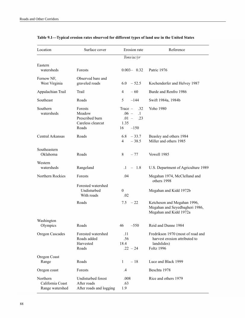
88
Roads and Other Corridors
Table 9.1—Typical erosion rates observed for different types of land use in the United States
Location Surface cover Erosion rate Reference
Tons/ac/yr
Eastern
watersheds Forests 0.003– 0.32 Patric 1976
Fernow NF, Observed bare and
West Virginia graveled roads 6.0 – 52.5 Kochenderfer and Helvey 1987
Appalachian Trail Trail 4 – 60 Burde and Renfro 1986
Southeast Roads 5 –144 Swift 1984a, 1984b
Southern Forests Trace – .32 Yoho 1980
watersheds Meadow .06 – .1
Prescribed burn .01 – .23
Careless clearcut 1.35
Roads 16 –150
Central Arkansas Roads 6.8 – 33.7 Beasley and others 1984
4 – 38.5 Miller and others 1985
Southeastern
Oklahoma Roads 8 – 77 Vowell 1985
Western
watersheds Rangeland .1 – 1.8 U.S. Department of Agriculture 1989
Northern Rockies Forests .04 Megahan 1974, McClelland and
others 1998
Forested watershed
Undisturbed 0 Megahan and Kidd 1972b
With roads .02
Roads 7.5 – 22 Ketcheson and Megahan 1996,
Megahan and Seyedbagheri 1986,
Megahan and Kidd 1972a
Washington
Olympics Roads 46 –550 Reid and Dunne 1984
Oregon Cascades Forested watershed .11 Fredrikson 1970 (most of road and
Roads added .56 harvest erosion attributed to
Harvested 18.4 landslides)
Roads .22 – 24 Foltz 1996
Oregon Coast
Range Roads 1 – 18 Luce and Black 1999
Oregon coast Forests .4 Beschta 1978
Northern Undisturbed forest .008 Rice and others 1979
California Coast After roads .63
Range watershed After roads and logging 1.9

89
Figure 9.2—Mean soil loss rates for four road surfaces before, during, and for 2 years after logging (based on Swift 1984a).
Chapter 9
installed, rights-of-way may continue to be sources of
sediment if revegetation or other erosion control practices
are not initiated (Gray and Garcia-Lopez 1994). Frequently,
off-road vehicle enthusiasts may use rights-of-way for
recreation. Also, mechanical and chemical control of
vegetation may reduce vegetative cover. Depending on the
site conditions, erosion rates from the compacted trails or
exposed rights-of-way may be similar to those of roads.
Trails for bicycling, walking, or horseback riding erode at
rates similar to roads (Leung and Marion 1996). The total
sediment delivered from these trails is generally lower,
however, because the total surface area of a narrow trail is
less than that of most roads.
Much of the sediment eroded from a right-of-way is rapidly
deposited below the right-of-way and never reaches a
stream. Rummer and others (1997) found no significant
sedimentation effects beyond the clearing limit of the road
in a bottomland hardwood study on a floodplain. Numerous
scientists have developed equations from field observations
to predict how far sediment will travel (Ketcheson and
Megahan 1996, McNulty and others 1995, Packer and
Christensen 1977, Swift 1986).
Various mitigation measures to reduce road erosion are
commonly prescribed by Federal and State agencies. The
most common methods include surfacing the road with
gravel, decreasing the spacing of cross drainage, locating
roads farther from streams, or limiting road gradients
(Burroughs and King 1989, Swift 1984a, Yoho 1980).
Table 9.2—Effectiveness of erosion mitigation techniques
Condition Reduction Reference
Percent
Erosion mat 74 – 99 Grace and others 1998
Seeding 82 – 95 Grace and others 1998
Grass on fillslope 46 – 81 Appelboom and others 1998
Straw and asphalt tack or 60 – 100 Burroughs and King 1989
erosion mats (depends
on percent cover)
Straw 60 – 80 Burroughs and King 1989
0
10
20
30
40
50
60
70
80
90
100
Prelogging Logging 1 year after
logging
2 years after
logging
Ero
sio
n r
ate
(to
n/a
cre
)
Soil
Grass
6-in. gravel
8-in. rock

90
Roads and Other Corridors
Treatment of cut and fillslopes has also been effective in
reducing sediment delivery from new roads (table 9.2)
(Burroughs and King 1989, Grace and others 1998).
Sediment production can be reduced by applying higher
quality gravel (Foltz and Truebe 1995) or by reducing the
pressure in vehicle tires on the road network (Foltz 1994).
The installation of vegetated filter strips or slash filter
windrows below fills, or sediment basins below culverts, are
also management options that have reduced sedimentation.
In climates with distinct wet seasons, seasonal closure of
roads may be a desirable option to prevent rutting and
severe erosion.
In an effort to reduce the impacts of roads and railroads in
watersheds, many government management agencies are
removing unwanted corridors. In many national forests,
watershed restoration is synonymous with removal of excess
roads (Elliot and others 1996). Moll (1996) presented an
overview of road closure and obliteration methods in the
Forest Service. He recommended that watershed managers
consider access, drainage, erosion risk, slope stability, and
revegetation when planning any road closure or obliteration.
Table 9.3 summarizes management options for decommis-
sioned roads. Elliot and others (1996) warn that the distur-
bances associated with road closure may cause more erosion
than simply abandoning a road that has been revegetated
and is hydrologically stable.
Surface erosion rates can drop significantly when roads are
closed. Figure 9.2 shows the relative impacts of different
road surfaces during the first 2 years after abandonment,
compared to erosion rates during construction and logging
(Swift 1984b). In the Oregon Cascades, Foltz (1996)
observed that during the first year of closure erosion rates
dropped from 4 to 0.5 tons per acre (9 to 1 Mg per hectare)
when marginal quality aggregate was applied, 20 to 2.5 tons
per acre (45 to 5.6 Mg per hectare) when good-quality
aggregate was applied. Erosion will often drop to back-
ground levels as the density of vegetation on an abandoned
road surface increases (Foltz 1996, Swift 1984b). Such a
decline is unlikely, however, if the abandoned road has
unvegetated surfaces and continues to concentrate runoff
water.
Several general principles can be applied to analyzing and
mitigating potential sediment sources from abandoned
corridors. The surface should be covered with vegetation. In
order to establish vegetation, it may be necessary to rip or
till the surface. In extreme cases, it may be necessary to add
topsoil. To encourage infiltration and revegetation, it may
be necessary to discourage off-road vehicle traffic by
installing permanent barriers to prevent wheeled access to
the corridor.
On abandoned roads, culverts can fail or become blocked,
causing ponding of water, embankment failure, and major
offsite sedimentation (Elliot and others 1994). Many older
roads or railroads were built with underdesigned culverts.
Some culverts were made from wood that is decaying or
metal that is corroding. In either case, most of these culverts
will eventually fail unless they are removed or replaced.
Culverts that are not regularly inspected can also become
blocked with woody debris or sediment. One of the most
common practices to minimize the risk of fill failure on
abandoned rights-of-way is to remove the culverts.
A number of prediction models have been developed to
estimate the amount of sediment that leaves forest roads.
Site-specific models were developed in the northern Rocky
Mountains by Forest Service hydrologists; the most recent is
the Watershed and Sediment Yield Model (WATSED) model
(U.S. Department of Agriculture, Forest Service 1990).
McNulty and others (1995) presented a Geographical
Information System-based method for predicting sediment
delivery from a road network, but they observed that
additional work with physically based models is necessary
to improve the prediction of sediment delivery from roads.
The physically based Water Erosion Prediction Project
(WEPP) model is under development for a wide range of
conditions including agriculture, range, and forest condi-
tions (Laflen and others 1997). Because it is physically
based, the model can be applied whenever the factors that
cause erosion can be adequately described. Elliot and Hall
(1997) have developed a set of input templates for forest
roads and other disturbances. Elliot and others (1999b)
developed simplified tools based on the WEPP model to aid
managers in estimating the impacts of climate, soil, and
topography on the delivery of sediment from roads. These
models are available on the Web at http://forest.moscowfsl.
wsu.edu/fswepp/.
Reliability and Limitations of Findings
Researchers worldwide have measured increased sedimenta-
tion from roads and similar disturbances. The magnitude of
erosion varies considerably with climate, but the relative
impacts of soil, topography, and management are generally
the same (Elliot and others 1999b). Observed erosion rates
are highly variable (table 9.1) due to the high natural
variability in the factors that cause erosion. Even a well-
designed erosion experiment frequently results in variations
from the mean of up to 50 percent. This high variability
should be considered when interpreting any research or
monitoring results, or any erosion prediction value. Manag-
ers should exercise caution when applying any model to an
area where it has not received some validation. Predictive
technology for one climate, soil, and topography does not

91
Chapter 9
translate well to other conditions unless the model is able to
incorporate those site-specific characteristics.
The technology to remove abandoned roads is well estab-
lished (Moll 1996). Numerous agencies including the Forest
Service (Moll 1996; U.S. Department of Agriculture, Forest
Service 1998) and the National Park Service2 have special-
ists to provide technical assistance in road closure, stabiliza-
tion, revegetation, and removal. Many abandoned roads and
railroads require site-specific prescriptions for reclamation.
The same level of design that went into creating some of
these roads may be required to remove them (Elliot and
others 1996). Although this design expertise is available, the
cost may be prohibitive.
Research Needs
1. Upland erosion and sedimentation are well understood.
The long-term impacts of trapping sediment on hillsides
between sites of disturbance and streams and movement
of sediment within and through stream networks are not
well understood. Future research on overland transport
and storage of sediment and transport and storage in
stream networks will enhance sedimentation prediction.
2. Reports related to problems associated with abandoned
roads and railroads focus specifically on culverts or mass
failures. Surface and channel erosion may be a chronic
source of sediment for many years. Thus, published
information is frequently limited to episodic problems
rather than solutions to chronic problems. There is a need
for research to determine the probability of a failure
occurring as well as the probability that no failure will
occur.2 Spreiter, T.A. 1999. Road closure experiences of the National ParkService. Presented at the Oregon and Washington engineering workshop;1999 March 9; Gleneden Beach, OR. Oral presentation.
Table 9.3—Management options for decommissioned roads
Option Comment
Close road with barriers, vegetation,
ditch, or removal of first segment Recreational users may still obtain access.
Rip road surface Runoff is reduced (Luce 1997). Instability may be
increased (Elliot and others 1996).
Revegetate road surface See table 9.2
Remove culverts and restore channels Mitigation may be necessary on bare, excavated
embankments or in channels; remaining road
segments may not be accessible for future
maintenance (Moll 1996).
Reshape road surface to be outsloping
or partially recontoured with regular
waterbars Moll 1996
Install rock buttresses to stabilize cut
and fillslopes Moll 1996
Remove, recontour, or obliterate road Expensive [$0.60 to 1.50 per lineal ft (Moll
prism 1996)] Increase revegetation rate by excavating
until the old topsoil is reacheda
Mitigate obliterated road prism with
slash, mulch, geotextile, or seeding Moll 1996
a Spreiter, T.A. 1999. Road closure experiences of the National Park Service. Presented at the Oregon and Washington
engineering workshop; 1999 March 9; Gleneden Beach, OR. Oral presentation.

92
Roads and Other Corridors
3. Research is also needed to determine risks of failure or
erosion for specific road networks.
4. There is a need to develop field techniques to assist road
and watershed managers to make better decisions on
which segments of a road network are at the greatest risk
of a failure that may impact off-site water quality as well
as other resources.
5. Another need is to develop tools to estimate the amount
of sediment that may come from road closure activities,
both from reshaping or removing the road prism, and
from removal of stream-crossing structures.
Key Points
1. Roads and similar corridors can be a major source of
sediment in a forested watershed.
2. Effective measures to reduce sedimentation include
surface gravel, careful design of roads and water cross-
ings, and removal of unwanted roads.
3. Abandoned roads may be sources of sediment if they
collect or divert surface runoff.
Hydrocarbons, Cations, and
Related Pollutants
Issues and Risks
Runoff from roads and similarly surfaced sites can contain a
host of hydrocarbons and other chemical pollutants,
adsorbed to sediments, as particles, or dissolved by the
runoff. These chemicals can find their way into surface and
subsurface water. Pesticides used to control unwanted weeds
can also be a source of pollution, and the reader should refer
to chapter 12 for further discussion.
Findings from Studies
Researchers have identified a range of chemicals in road
runoff (tables 9.4, 9.5). Some of the pollutants are from the
road material itself, some occur in the soil and rock on the
site and are released during construction or subsequent
erosion, and many are from vehicles. Traffic and road
surfacing may contribute undesirable cations, hydrocarbons,
and metals to surface and subsurface water (Maltby and
others 1995, Mungur and others 1994). Most studies on the
impact of roads and similar disturbances have focused on
heavily traveled roads such as major freeways (Mungur and
others 1994). If water source areas contain major roads,
runoff treatment may be necessary to ensure that undesirable
hydrocarbons do not enter the water supply.
Cations released from a road may have a buffering effect on
the runoff acidity, which may be beneficial in acid rain
areas. Morrison and others (1995) measured pH values from
6.0 to 7.0 in road runoff from small storms, compared to the
average rainfall pH of 4.1.
Ions from deicing or dust control chemicals are common
pollutants from road surfaces (Church and Friesz 1993,
Pugh and others 1996). Road salt contamination of shallow
ground water has become a serious problem, particularly in
the Northeast and Midwest (Church and Friesz 1993).
Church and Friesz (1993) state that during a 7-year period in
Massachusetts, there were complaints from 100 of the 341
municipalities about road salt contamination. Nationally,
about $10 million are spent each year for prevention or
remediation of problems associated with road salt contami-
nation. Surface water is less vulnerable to such contamina-
tion than ground water, because there tends to be much
greater dilution and mixing in turbulent channels carrying
runoff from roads (Jongedyk and Bank 1999). Calcium
magnesium acetate and potassium acetate are deicing
chemicals with less serious environmental consequences
than sodium chloride because they contain weak biodegrad-
able acids. Sodium chloride, calcium chloride, and magne-
sium chloride, however, leave residues of chloride ions that
may contaminate ground water (Jongedyk and Bank 1999).
Some of these ions (calcium, magnesium, and potassium)
can enhance vegetation growth along highways (Pugh and
others 1996). In some cases, elevated levels of deicing
cations such as sodium in the road runoff, may be adsorbed
by the soils near the road, and pose no further concern to the
aquatic ecosystem (Shanley 1994). Pugh and others (1996)
observed that ion concentrations from an adjacent interstate
highway decreased exponentially with distance from the
road in a peat bog. Although many thousands of tons of salt
are spread annually on highways, because of dilution, salts
in runoff are not likely to be a major source of pollution for
drinking water except where they use shallow ground water
even though impacts on the aquatic ecosystem may be great.
Road dust can transport unwanted chemicals to surface
water. Christensen and others (1997) observed recent
accumulations of polycyclic aromatic hydrocarbons (PAH’s)
in a Wisconsin stream, and identified dust from nearby roads
as the source of the pollutant.
Oil-based dust suppressants may be environmentally more
risky than salt-based products. A literature search for the
Forest Service (Heffner 1997) found reports that calcium
and magnesium chloride showed some toxicity towards

93
Table 9.5—Mean concentrations of a number of
pollutants in highway runoff in Minnesota
Pollutant Range Mean
- - - - - Milligrams per liter - - - - - -
Total nitrogen 0.6 – 8.14 1.67
Chloride 1 – 46 000 1 802
Sulphate 5 – 650 45
Sodium 2 – 67 000 3 033
Total phosphorous .06 – 7.8 .6
BOD 1 – 60 12.6
COD 2 – 3 380 207
Total suspended solids 8 – 950 118
Total dissolved solids 22 – 81 700 10 440
- - - - - Micrograms per liter - - - - - -
Chromium 1.5 – 110 13
Copper 3 – 780 47
Iron 180 – 45 000 4 162
Lead 11 – 2 100 207
Zinc 10 – 1 200 174
Nickel 1 – 57 10
Cadmium .2 – 12 1.7
Mercury .08 – 5.6 .49
Aluminum 30 – 14 000 2 694
Arsenic .1 – 340 19
BOD = biological oxygen demand; COD = chemical oxygen demand.
Source: Thomson and others 1997.
Chapter 9
plants, whereas ligninsulfonate increased water biological
oxygen demand. The study concluded:
based on the literature review and typical application
rates for dust abatement, the effects of these com-
pounds on plants and animals would be negligible.
For the purposes that the Forest Service uses these
compounds, the selection of one over another would
be more dependent on cost, availability, and local
conditions than effects to the environment.
Some dust inhibitors may also decrease road erosion,
decreasing the likelihood of off-site transport of sediment
and related pollutants (Ice 1982).
Chemicals used to preserve utility poles and railway
crossties are potential sources of pollution. Wan (1994)
found that concentrations of PAH’s in the soil were higher in
the immediate vicinity of utility poles than on surrounding
farm or rangeland. Soil concentrations of PAH’s dropped
rapidly from 550 micrograms (µg) per liter to 23.2 µg per
liter within 13 feet (4 meters) of a treated pole. Background
levels were between zero and 0.8 µg per liter. Such findings
emphasize the importance of maintaining vegetated buffers
to reduce transport by erosion of contaminated soil between
rights-of-way and any sensitive water resources.
Measuring concentrations of many pollutants is tedious and
expensive. To reduce the cost, surrogate relationships have
been developed between more easily measured pollutants,
such as suspended solids (mainly sediment) or dissolved
Table 9.4—Pollutants that have been observed in runoff from road surfaces
Pollutant Comment Reference
Cd, Cu, Pb, Zn Treated in wetlands Mungur and others 1994
Highway deicing salt Na adsorbed in soil Shanley 1994
Cu, Zn, hydrocarbons, PAH’s Accumulated in aquatic biota Maltby and others 1995
PAH’s Altered aquatic communities Boxall and Maltby 1997
Ca, Mg, Na, K, Cl Captured in peat bogs Pugh and others 1996
Total petroleum
hydrocarbons, Pb, Zn Reduced by vegetation Ellis and others 1994
Heavy metals, petroleum hydro- Treatment ponds can remove Karouna-Renier and Sparling 1997
carbons, pesticides, sediment, up to 95 percent of pollutants.
nutrients
Ca = calcium; Cd = cadmium; Cl = chloride; Cu = copper; K = potassium; Mg = magnesium; Na = sodium; PAH’s = polycyclic aromatic
hydrocarbons; Pb = lead; Zn = zinc.

94
Roads and Other Corridors
solids and other pollutants that are difficult to measure
(Thomson and others 1997). Such surrogates may be useful
if relationships were developed for nearby conditions, but
they become less reliable when extrapolated to other
regions.
Gilson and others (1994) completed research on the effec-
tiveness of filter systems for highway runoff to improve
surface water quality in the karst terrain in Texas. They
found that some alternatives to sand filters have higher
adsorptive capacities initially, but filtration efficiencies
tended to approach that of sand after several runoff events.
A Virginia study found that highways in karst areas should
be located to avoid polluting surface water that drains into
caves (Hubbard and Balfour 1993). This study found raw
sewage and petroleum fumes in the cave system. Keith
(1996) described extra precautions on road location and
drainage designs that were taken in Indiana to minimize the
ground water impact of a new road design in a karst area.
Pollutants in runoff can be trapped in natural or artificial
wetland areas (Ellis and others 1994, Karouna-Renier and
Sparling 1997, Mungur and others 1994). Karouna-Renier
and Sparling (1997) found that such treatment systems could
remove up to 95 percent of metals, nutrients, and sediment.
Monitoring of the performance of such areas is necessary to
ensure that they are functioning as desired (Startin and
Lansdown 1994).
Another treatment method is a partial exfiltration trench.
This type of device filters out the suspended solids that carry
many of the undesirable metals and hydrocarbons from road
surfaces (Sansalone and Buchberger 1995). The trench
improved the quality of both rainfall and snowmelt runoff
from roads. Because of the wide range of runoff rates,
however, multiple treatment methods may be necessary to
decrease the pollutant load from large as well as small
storms (Romero-Lozano 1995). Detention basins are needed
to catch the first flush of highly polluted runoff. A filtration
system is needed to treat the runoff from later in the storm,
which is likely to be at a higher flow rate, but requires less
treatment.
Sediment basins and similar structures built to contain
polluted road runoff can become sources of pollution
through seepage into the ground, or through other forms of
hydraulic or structural failure. In either case, sediments with
large amounts of adsorbed chemicals can enter a stream.
The pollutants can become concentrated in these basins,
increasing the risk of offsite pollution (Grasso and others
1997, Morrison and others 1995). Grasso and others (1997)
observed a lead content of 1392 milligrams per kilogram on
one site and recommended soil washing be carried out to
prevent offsite pollution. One of the best defenses against
such risks is cleaning and maintaining such structures to
minimize the risk of failure.
Past designs of runoff structures tended to collect water and
route it directly to a stream. New designs that disperse water
to ensure greater infiltration and onsite attenuation of
pollutants can improve runoff quality (Elliot and Tysdal
1999, Li and others 1998). Not all sites lend themselves to
this approach, particularly where rights-of-way are limited.
Another recent innovation to reduce offsite pollution from
roads and similar areas is to surface them with permeable
pavement (Church and Friesz 1993). Permeable pavement
combined with high-infiltration shoulders significantly
decreased salt content in nearby ground water (Church and
Friesz 1993, Jongedyk and Bank 1999). European research-
ers found that permeable pavement significantly reduced
outflow levels of lead and suspended solids.
Reliability and Limitations of Findings
Much of the research associated with chemical pollution
from roads has taken place near large urban centers. The
findings are generally reliable for their locality, but care
needs to be taken in extrapolating to other conditions,
particularly nonurban areas. The water-quality risks associ-
ated with hydrocarbon pollution are closely linked to the
density of traffic. Watersheds with minimal traffic are
unlikely to experience any of the problems discussed. These
results should only be applied to more remote watersheds
with caution and some form of monitoring.
Research Need
Pollution from main roads that cross sensitive forest and
grassland watersheds should be measured. Quantitative data
are needed on the benefits of dust abatement chemicals for
reducing erosion and pollution of streams near roads.
Key Point
Many pollutants from vehicles, deicing and dust abatement
chemicals, and road surfacing material have been measured
in runoff from roads. Most of these measurements have been
from roads with heavy traffic. Some level of monitoring
may be necessary to determine pollution problems. Levels
of pollution can often be related to levels of easily measured
sediment concentration. Some cations in runoff may be
beneficial in buffering acid rain. There are methods to
collect and treat or to harmlessly disperse polluted road
runoff.

95
Chapter 9
Fuels and Other Contaminants
from Accidental Spills
Issues and Risks
Accidents are rare on low-use roads and other rights-of-way
in remote watersheds. Risks of an accident causing contami-
nation spills are related to the traffic density, quality of road,
and frequency of contaminant transport. Railroads pose
similar risks, particularly on aging lines, or on busy routes
linking industrial centers.
Findings from Studies
Hazardous chemical spills from vehicle accidents can pose a
direct, acute threat of contamination to streams. Risk
analysis models have been developed for busy paved roads
in nonmountainous terrain, but these models are seldom
applicable to low traffic, remote watersheds. Chemicals that
may be spilled include fuel, fertilizer, pesticides, and mining
chemicals (U.S. Department of Agriculture, Forest Service
1998). Airfields can often be sources of ground water
contamination due to spills of fuels and other material
(Levine and others 1997).
Accidents may occur anywhere along a given road or
railroad, but stream crossings and bridges tend to be
frequent sites of accidents due to damage by floods, or a
narrowing of the roadway. Whether the pollutant is able to
reach a nearby stream is an important concern. Spills at
stream crossings have a high likelihood of reaching surface
water because of its close proximity. Frequently, transport of
the pollutant overland, or through the soil, depends on the
local climate, season, and hydrology.
Reliability and Limitations of Findings
There is little information available on the risk of accidental
spills in remote areas. Whatever information can be found is
likely to be site-specific, and judgment must be used to
apply it elsewhere. Watershed managers will need to
develop their own set of potential risks, based on local
conditions. Along with those risks, they will need to develop
a set of potential mitigation measures, both in the water
source area, and in the treatment system.
Ability to Address Issues
Most counties have established committees to address local
emergencies or disasters. An accident that impacts a local
water supply is a prime example of such an emergency.
Water supply managers should work with local emergency
or disaster committees or services to ensure that mitigation
plans and equipment are in place to deal with toxic spills
that may occur near a water source.
Research Need
Because of the site-specific nature of this risk, it is difficult
to define a broad research activity for remote watersheds. It
is likely that research will continue to study risks associated
with busier roads, so monitoring of those results for applica-
tion to remote watersheds may be beneficial.
Key Point
The risk of vehicle accidents and spills depends on road
hazards and traffic volume. Watershed managers need to
evaluate risks on a given watershed and develop prevention
or mitigation measures specific to their own conditions.
Pipeline Failures
Issues and Risks
Pipelines carrying a wide range of substances, including
drinking water, sewage, and petroleum products, can fail,
leading to pollution of both surface water and ground water.
In the past 15 years, about 200 oil pipeline failures have
occurred per year, with an average net loss of about 600
barrels (95 cubic meters) for each spill (U.S. Department of
Transportation 1999).
Findings from Studies
Pipelines tend to have fewer accidents and injuries than
other modes of transport (Jones and Wishart 1996). To
minimize pollution impacts, most modern pipeline systems
are equipped with devices to quickly shut down pumping if
a change in flow or pressure is sensed (Ariman 1990).
A number of disturbances increase the likelihood of pipeline
accidents (fig. 9.3). Road or construction accidents and
damage from boulders are common external causes of
damaged pipelines (Driver and Zimmerman 1998, Stalder
1997). Areas prone to severe erosion, landslides, and
earthquakes tend to have more accidents (Ariman 1990,
Gray and Garcia-Lopez 1994, Hart and others 1995). For
example, Hart and others (1995) predicted that the probabil-
ity of rupture for a pipeline in California increased from 0.0
for earthquakes with a magnitude below 5 to 1.0 for
earthquake magnitudes greater than 6.0. They also predicted
other probabilities of failure based on pipe length and
installation. They recommended numerous design measures
including depth of burial, trench design, and pipe wall
thickness, to minimize failure due to earthquakes.

96
Corrosion24%
Other30%
Equipment6%
Damage26%
Pipe4%
Operation5%
Welds5%
Figure 9.3—Summary of causes of pipeline accidents in 1998 in the United
States (U.S. Department of Transportation 1999).
Roads and Other Corridors
Pipelines sometimes fail at river crossings due to erosion of
the streambank or bottom (Doeing and others 1995, Teal and
others 1995). Pipelines carrying sewage and industrial
wastes are frequently located in floodplains and are at
particular risk from flood damage, or from overloading due
to high runoff rates. Disturbances in a watershed, such as a
fire, may cause landslides that lead to pipeline failure.
Failure of water supply pipelines or canals can lead to
considerable erosion if controls to monitor flow conditions
are not in place.
Soil shrinking and swelling and freezing and thawing can
lead to pipeline fatigue and premature failure. Corrosion due
to electrolysis (Stalder 1997) and stress corrosion cracking
can also occur on older pipelines (Wilson 1996). Above-
ground pipelines can fail due to wind fatigue (Honegger and
others 1985). Any pipeline may experience seam failure
(Yaorong and others 1996).
Risk assessment models to aid in pipeline design and
operation have been developed (Hart and others 1995,
Nessim and Stephens 1998). These models can identify
segments of pipe most at risk of failure, and maintenance
can be concentrated on those segments. Risk rates of 0.0022
spills per mile per year are quoted in one environmental
assessment (U.S. Department of the Interior, Bureau of Land
Management 1978).
Table 9.6 shows the extent of contamination from 53 oil
pipeline spills. The extent depends on the pipeline character-
istics and on the soils and terrain. Risks of failure from
normal, predictable events can be reduced to almost zero
with adequate pipeline monitoring (Stalder 1997). In
addition, technologies have been developed to mitigate the
impacts of spills quickly and effectively (Sittig 1978).
Pipeline failures can pollute ground water as well as surface
water. Petroleum products tend to float on ground water, but
the processes associated with breakdown of oil underground
are not well understood. Underground methane generation
by anaerobic bacteria is common after a pipeline break.
Substantial amounts of the volatile petroleum hydro-
carbons are transported from the surface of the water
table through the unsaturated zone as vapor, which
subsequently dissipates to the atmosphere or is
biodegaded (Revesz and others 1996).
Eganhouse and others (1996) observed that an underground
breakdown process from microbial degradation leads to the
detection of a plume containing aliphatic, aromatic, and
alicyclic hydrocarbons.
Pipelines carrying water and sewage may also be present on
watersheds. Although the same principles of failure apply to
these pipelines, they are generally not as well monitored and
may be older and more prone to failure.
Reliability and Limitations of Findings
These findings are generally reliable because much of the
pipeline industry receives close government scrutiny.
Pipeline failures tend to be mechanical and predictable and
findings are generally applicable to local conditions.
Current technology can address the risks associated with
pipeline failure. Technologies to minimize pipeline failure
are well established in the petroleum industry, as are
controls to minimize pollution of surface and ground water
should a failure occur. These same technologies can also be
applied to other pipelines in sensitive watersheds. Managers
of watersheds containing pipelines should work with
Table 9.6—Extent of soil contamination by 53 oil spills of
various sizes in Alberta, Canada
Average Average Average film
volume area thickness
Barrels Ft2
In.
54 8,000 0.4
880 70,000 .8
13,200 600,000 1.6
Barrel = 42 gallons of petroleum.
Source: U.S. Department of the Interior, Bureau of Land Management 1978.

97
Chapter 9
pipeline managers to minimize risks to water supplies. In
addition, the U.S. Department of Transportation has an
Office of Pipeline Safety (OPS) to assist in addressing risks
associated with pipelines. One of its responsibilities is to
identify areas that are unusually sensitive to a hazardous
liquid pipeline release. The OPS has an ongoing program
that may assist watershed managers in risk management (see
Web site).
Research Need
The oil industry has developed sophisticated systems for
managing pipelines. There is a need to develop similar, but
less costly, technologies for water and sewer pipelines in
sensitive watersheds. The fate of oil pollution in the ground
is not well understood, and further research is needed to
better understand the chemical and biological processes
associated with degradation of petroleum products on and in
the soil.
Key Point
Causes of failures on petroleum pipelines are well under-
stood, and controls are generally in place to minimize
environmental risks of failures. Such measures are less
developed for water and sewage pipelines, so the risks of the
failure of such systems may be higher.
Literature Cited
Appelboom, T.W.; Chescheir, G.M.; Skaggs, R.W.; Hesterberg, D.L.
1998. Evaluating management practices for reducing sediment
production from forest roads. American Society of Agricultural
Engineers annual international meeting; 1998 July 12–16; Orlando, FL.
Pap. 987025. St. Joseph, MI: American Society of Agricultural
Engineers. 11 p.
Ariman, T. 1990. Seismic vulnerability of crude oil pipelines. Pipeline and
Gas Journal. 217(July): 22–24.
Beasley, R.S.; Miller, E.L.; Gough, S.C. 1984. Forest road erosion in the
Ouachita Mountains. In: Peters, P.A.; Luchok, J., eds. Mountain logging
symposium proceedings; 1984 June 5–7; Morgantown, WV.
Morgantown, WV: West Virginia University: 203–213.
Beschta, R.L. 1978. Long-term patterns of sediment production following
road construction and logging in the Oregon coast range. Water
Resources Research. 14(8): 1011–1016.
Boxall, A.B.A.; Maltby, L. 1997. The effects of motorway runoff on
freshwater ecosystems: 3. Toxicant confirmation. Archives of Environ-
mental Contamination and Toxicology. 33(1): 9–16.
Burde, J.H.; Renfro, J.R. 1986. Use impacts on the Appalachian trail. In:
Lucas, R.C., comp. Proceedings—national wilderness research
conference: current research; 1985 June 5–7; Fort Collins, CO. Gen.
Tech. Rep. INT–212. Ogden, UT: U.S. Department of Agriculture,
Forest Service, Intermountain Research Station: 138–143.
Burroughs, E.R., Jr.; King, J.G. 1989. Reduction of soil erosion on forest
roads. Gen. Tech. Rep. INT–264. Ogden, UT: U.S. Department of
Agriculture, Forest Service, Intermountain Research Station. 21 p.
Burroughs, E.R., Jr.; Marsden, M.A. 1972. Volume of snowmelt
intercepted by logging roads. Journal of the Irrigation and Drainage
Division. March: 1–12.
Christensen, E.R.; Li., A.; Razak, I.A.A. [and others]. 1997. Sources of
polycyclic aromatic hydrocarbons in sediments of the Kinnickinnic
River, Wisconsin. Journal of Great Lakes Research. 23(1): 61–73.
Church, P.E.; Friesz, P.J. 1993. Effectiveness of highway drainage
systems in preventing road-salt contamination of groundwater:
preliminary findings. Transp. Res. Rec. 1420. Washington, DC: National
Academy Press: 56–60.
Doeing, B.J.; Bradley, J.B.; Carreon, S. 1995. Avoiding pipeline failures
at waterway crossings. Part 1: scour assessment methods. In: Proceed-
ings of the 2d international conference on advances in underground
pipeline engineering; 1995 June 25–28; Bellvue, WA. New York:
American Society of Civil Engineers: 65–76.
Driver, R.G.; Zimmerman, T.J.E. 1998. Limit States’ approach to the
design of pipelines for mechanical damage. In: Proceedings of the 17th
international conference on offshore mechanics and arctic engineering—
OMAE; 1998 July 5–9; Lisbon, Portugal. Fairfield, NJ: American
Society of Mechanical Engineers: 1–14.
Eganhouse, R.P.; Dorsey, T.F.; Phinney, C.S.; Westcott, A.M. 1996.
Processes affecting the fate of monoaromatic hydrocarbons in an aquifer
contaminated by crude oil. Environmental Science and Technology.
30(11): 3304–3312.
Elliot, W.J.; Foltz, R.B.; Luce, C.H. 1999a. Modeling low-volume road
erosion. In: Proceedings of the 7th international conference on low-
volume roads; 1999 May 23–27; New Orleans. Transp. Res. Rec. 1652.
Washington, DC: National Academy Press. (2): 244–250.
Elliot, W.J.; Foltz, R.B.; Luce, C.H.; Koler, T.E. 1996. Computer-aided
risk analysis in road decommissioning. In: McDonnell, J.J.; Stribling,
J.B.; Neville, L.R.; Leopold, D.J., eds. Proceedings of the AWRA annual
symposium on watershed restoration management: physical, chemical,
and biological considerations; 1996 July 14–17; Syracuse, NY. Herndon,
VA: American Water Resources Association: 341–350.
Elliot, W.J.; Hall, D.E. 1997. Water erosion prediction project (WEPP)
forest applications. Gen. Tech. Rep. INT–365. Ogden, UT: U.S.
Department of Agriculture, Forest Service, Intermountain Research
Station. 11 p.
Elliot, W.J.; Hall, D.E.; Graves, S.R. 1999b. Predicting sedimentation
from forest roads. Journal of Forestry. 97(8): 23–29.
Elliot, W.J.; Koler, T.E.; Cloyd, J.C.; Philbin, M. 1994. Impacts of
landslides on an ecosystem. Pap. 947517. Presented at the 1994
American Society of Agricultural Engineers international winter
meeting; 1994 December 13–16; Atlanta. St. Joseph, MI: American
Society of Agricultural Engineers. 10 p.
Elliot, W.J.; Tysdal, L.M. 1999. Understanding and reducing erosion from
insloping roads. Journal of Forestry. 97(8): 30–34.
98
Roads and Other Corridors
Ellis, J.B.; Revitt, D.M.; Shutes, R.B.E.; Langley, J.M. 1994. The
performance of vegetated biofilters for highway runoff control. In:
Hamilton, R.S.; Revitt, D.M.; Harrison, R.M.; Monzon-de-Caceres, A.,
eds. Proceedings of the 4th international symposium on highway
pollution; 1992 May 18–22; Madrid, Spain. London: Middlesex
University: 543–550.
Foltz, R.B. 1994. Sediment reduction from the use of lowered tire
pressures. Central tire inflation systems—managing the vehicle to
surface (SP–1061). Pap. 942244. Warrendale, PA: Society of Automotive
Engineers: 47–52.
Foltz, R.B. 1996. Traffic and no-traffic on an aggregate surfaced road:
sediment production differences. In: Proceedings of the seminar of
environmentally sound forest roads and wood transport; 1996 June
17–22; Sinaia, Romania. Rome: Food and Agriculture Organization of
the United Nations: 195–204.
Foltz, R.B.; Truebe, M.A. 1995. Effect of aggregate quality on sediment
production from a forest road. In: Proceedings of the 6th international
conference on low-volume roads; 1995 June 25–29; Minneapolis.
Washington, DC: National Academy Press: 49–57.
Fredrickson, R.L. 1970. Erosion and sedimentation following road
construction and timber harvest on unstable soils in three small western
Oregon watersheds. Res. Pap. PNW–104. Portland, OR: U.S. Depart-
ment of Agriculture, Forest Service, Pacific Northwest Forest and Range
Experiment Station. 15 p.
Gilson, M.P.; Maliva, J.F.; Charbeneau, R.J.; Ward, G.H. 1994.
Highway runoff studied. Water Environment & Technology. 6(8): 37–38.
Grace, J.M., III; Rummer, R.; Stokes, B.; Wilhoit, J. 1998. Evaluation
of erosion control techniques on forest roads. Transactions of the
American Society of Agricultural Engineers. 4(2): 383–391.
Grasso, D.; Butkus, M.A.; O’Sullivan, D.; Nikolaidis, N.P. 1997. Soil-
washing design methodology for a lead-contaminated sandy-soil. Water
Research. 31(12): 3045–3056.
Gray, D.H.; Garcia-Lopez, M. 1994. Protecting a pipeline. Civil
Engineering. 64(12): 44–47.
Hart, J.D.; Row, D.G.; Drugovich, G. 1995. Structural analysis and risk
assessment of the All American pipeline at the San Andreas fault
crossing. In: American Society of Mechanical Engineers, petroleum
division PD pipeline engineering 1995: Proceedings of the energy-
sources technology conference and exhibition; 1995 January 29–
February 1; Houston. New York: American Society of Mechanical
Engineers: 1–15.
Heffner, K. 1997. Water quality effects of three dust-abatement com-
pounds. U.S. Department of Agriculture, Forest Service. Engineering
Field Notes. 29: 35–43.
Honegger, D.G.; Nyman, D.J.; Nyman, K.J. 1985. Wind induced fatigue
damage estimated for surface oil pipelines in the Arctic. Oil and Gas
Journal. 83(July): 49–53.
Hubbard, D.A., Jr.; Balfour, W.M. 1993. An investigation of engineering
and environmental concerns relating to proposed highway construction
in a karst terrain. Environmental Geology. 22(4): 326–329.
Ice, G. 1982. An assessment of the use of lignosulfonates and possible
water quality impacts to forest streams. Corvallis, OR: National Council
of the Paper Industry for Air and Stream Improvement. 3 p.
Idaho Division of Environmental Quality. 1997. Paradise Creek TMDL
water body assessment and total maximum daily load. Lewiston, ID:
Idaho Division of Environmental Quality, Lewiston Regional Office.
72 p.
Jones, E.G.; Wishart, D.M. 1996. Pipelining in a changing competitive
environment. In: Proceedings of the 1st international pipeline conference;
1996 June 9–13; Calgary, Canada. New York: American Society of
Mechanical Engineers: 55–62.
Jones, J.A.; Grant, G.E. 1996. Peak flow responses to clear-cutting and
roads in small and large basins, western Cascades, Oregon. Water
Resources Research. 32(4): 959–974.
Jones, J.A., Swanson, F.J.; Wemple, B.C.; Snyder, K.U. [In press]. Road
and stream network interactive effects on hydrology and geomorphology
in western Oregon. Conservation Biology.
Jongedyk, H.; Bank, F. 1999. Is highway runoff a serious problem?
Federal Highway Administration Environmental Technology Brief.
McLean, VA: U.S. Department of Transportation. 9 p. [Available on the
Web at: http://www.tfhrc.gov/hnr20/runoff/runoff.htm].
Karouna-Renier, N.K.; Sparling, D.W. 1997. Toxicity of stormwater
treatment pond sediments to Hyalella azteca (Amphipoda). Bulletin of
Environmental Contamination and Toxicology. 58(4): 550–557.
Keith, J.H. 1996. Runoff treatment systems reduce highway-related
impacts in the Indiana karst. Land-water. 40(3): 12–16.
Ketcheson, G.L.; Megahan, W.F. 1996. Sediment production and
downslope sediment transport from forest roads in granitic watersheds.
Res. Pap. INT–486. Ogden, UT: U.S. Department of Agriculture, Forest
Service, Intermountain Research Station. 11 p.
Kochenderfer, J.N.; Helvey, J.D. 1987. Using gravel to reduce soil losses
from minimum-standard forest roads. Journal of Soil and Water
Conservation. 42(1): 46–50.
Laflen, J.M., Elliot, W.J.; Flanagan, D.C. [and others]. 1997. WEPP—
Predicting water erosion using a process-based model. Journal of Soil
and Water Conservation. 52(2): 96–102.
Leung, Y.; Marion, J.L. 1996. Trail degradation as influenced by
environmental factors: a state-of-the-knowledge review. Journal of Soil
and Water Conservation. 51(2): 130–136.
Levine, A.D.; Libelo, E.L.; Bugna, G. [and others]. 1997. Biogeochemi-
cal assessment of natural attenuation of JP–4-contaminated groundwater
in the presence of fluorinated surfactants. Science of the Total Environ-
ment. 208(3): 179–195.
Li, J.; Orland, R.; Hogenbirk, T. 1998. Environmental road and lot
drainage designs: alternatives to the curb-gutter-sewer system. Canadian
Journal of Civil Engineering. 25(1): 26–39.
Luce, C.H. 1997. Effectiveness of road ripping in restoring infiltration
capacity of forest roads. Restoration Ecology. 5(3): 265–270.
Luce, C.H.; Black, T.A. 1999. Sediment production from forest roads in
western Oregon. Water Resources Research. 35(8): 2561–2570.
Maltby, L.; Boxall, A.B.A.; Forrow, D.M. [and others]. 1995. The effects
of motorway runoff on freshwater ecosystems. 2. Identifying major
toxicants. Environmental Toxicology and Chemistry. 14(6): 1093–1101.

99
McClelland, D.E.; Foltz, R.B.; Falter, C.M. [and others]. 1998. The
relative effects of landslides resulting from episodic storms on a low-
volume road system in northern Idaho. U.S. Department of Agriculture,
Forest Service. Engineering Field Notes. 30: 7–22.
McNulty, S.; Swift, L., Jr.; Hays, J.; Clingenpeel, A. 1995. Predicting
watershed erosion production and over-land sediment transport using a
GIS. In: Carrying the torch for erosion control: an olympic task.
Proceedings of the 26th international erosion control association
conference; 1995 February 28–March 3; Atlanta. Steamboat Springs,
CO: International Erosion Control Association: 397–400.
Megahan, W.F. 1974. Erosion over time on severely disturbed granitic
soils: a model. Res. Pap. INT–156. Ogden, UT: U.S. Department of
Agriculture, Forest Service, Intermountain Forest and Range Experiment
Station. 26 p.
Megahan, W.F. 1983. Hydrologic effects of clearcutting and wildfire in
steep granitic slopes in Idaho. Water Resources Research. 19(3):
811–819.
Megahan, W.F.; Kidd, W.J. 1972a. Effect of logging roads on sediment
production rates in the Idaho batholith. Res. Pap. INT–123. Ogden, UT:
U.S. Department of Agriculture, Forest Service, Intermountain Forest
and Range Experiment Station. 14 p.
Megahan, W.F.; Kidd, W.J. 1972b. Effects of logging and logging roads
on erosion and sediment deposition from steep terrain. Journal of
Forestry. 70(3): 136–141.
Megahan, W.F.; Seyedbagheri, K.A. 1986. Construction phase sediment
budget for forest roads on granitic slopes in Idaho. In: Drainage basin
sediment delivery; Proceedings of a conference; 1986 August 4–8;
Albuquerque, NM. IAHS Publ. 159; Wallingford, UK: International
Association for Hydrological Sciences: 31–39.
Miller, E.L.; Beasley, R.S.; Covert, J.C. 1985. Forest road sediments:
production and delivery to streams. In: Blackmon, B.G., ed. Proceedings
of forestry and water quality: a mid-South symposium; 1985 May 8–9;
Little Rock, AR. Fayetteville, AR: University of Arkansas: 164–175.
Moll, J.E. 1996. A guide for road closure and obliteration in the Forest
Service. San Dimas, CA: U.S. Department of Agriculture, Forest
Service, San Dimas Technology and Development Center. 49 p.
Morrison, G.M.; Revitt, D.M.; Ellis, J.B. 1995. The gully pot as a
biochemical reactor. Water Science and Technology. 31: 229–236.
Mungur, A.S.; Shutes, R.B.E.; Revitt, D.M.; House, M.A. 1994. An
assessment of metal removal from highway runoff by a natural wetland.
In: Kadlec, R.H.; Brix, H., eds. Wetland systems for water pollution
control 1994: Selected proceedings for the 4th international conference
on wetland systems for water pollution control; 1994 November 6–10;
Guangzhou, China. London: Middlesex University, Urban Pollution
Research Center: 169–175.
Nessim, M.; Stephens, M. 1998. Quantitative risk-analysis model guides
maintenance budgeting. Pipe Line & Gas Industry. 81(6): 33–38.
Packer, P.E.; Christensen, G.F. 1977. Guides for controlling sediment
from secondary logging roads. Ogden, UT: U.S. Department of
Agriculture, Forest Service, Intermountain Forest and Range Experiment
Station; Missoula, MT: Northern Region. 41 p.
Patric, J.H. 1976. Soil erosion in the eastern forest. Journal of Forestry.
74: 671–677.
Pugh, A.L., IV; Norton, S.A.; Schauffler, M. [and others]. 1996.
Interactions between peat and salt-contaminated runoff in Alton Bog,
Maine, U.S.A. Journal Hydrology Amsterdam. 182(1–4): 83–104.
Reid, L.M.; Dunne, T. 1984. Sediment production from forest road
surfaces. Water Resources Research. 20(11): 1753–1761.
Revesz, K.; Coplen, T.; Baedecker, M.J. [and others]. 1996. Investiga-
tion of methane production and consumption by use of stable isotopes.
In: Isotopes in water resources management. Vienna, Austria: Interna-
tional Atomic Energy Agency: 381–387.
Rice, R.M.; Tilley, F.B.; Datzman, P.A. 1979. A watershed’s response to
logging and roads: south fork of Caspar Creek, California, 1967–1976.
Res. Pap. PSW–146. Berkeley, CA: U.S. Department of Agriculture,
Forest Service, Pacific Southwest Forest and Range Experiment Station.
12 p.
Robinson, E.G.; Mills, K.; Paul, J. [and others]. 1999. Storm impacts
and landslides of 1996. For. Res. Tech. Rep. 4. Salem, OR: Oregon State
Department of Forestry. 145 p.
Romero-Lozano, J. 1995. Highway design considers stormwater drainage
and treatment options. Public Works. 126(1): 32–33.
Rummer, B.; Stokes, B.; Lockaby, G. 1997. Sedimentation associated
with forest road surfacing in a bottomland hardwood ecosystem. Forest
Ecology and Management. 90(2–3): 195–200.
Sansalone, J.J.; Buchberger, S.G. 1995. An infiltration device as a best
management practice for immobilizing heavy metals in urban highway
runoff. Water Science Tech. 32(1): 119–125.
Shanley, J.B. 1994. Effects of ion exchange on stream solute fluxes in a
basin receiving highway deicing salts. Journal of Environmental Quality.
23(5): 977–986.
Sittig, M. 1978. Petroleum transportation and production: oil spill and
pollution control. Park Ridge, NJ: Noyes Data Corporation. 360 p.
Sonett, M.L. 1999. Integrated surface management for pipeline construc-
tion: the mid-America pipeline company four corners project. In: Finch,
D.M.; Whitney, J.C.; Kelly, J.F.; Loftin, S.R., eds. Proceedings of the
workshop on Rio Grande ecosystems: linking land, water, and people
toward a sustainable future for the middle Rio Grande Basin; 1998 June
2–5; Albuquerque, NM. Publ. RMRS–P–7. Fort Collins, CO: U.S.
Department of Agriculture, Forest Service, Rocky Mountain Research
Station: 180–183.
Stalder, F. 1997. Pipeline failures. Materials Science Forum. 247: 139–146.
Startin, J.; Lansdown, R.V. 1994. Drainage from highways and other
paved areas: methods of collection, disposal, and treatment. Journal of
Institute of Water and Environmental Management. 8(5): 518–526.
Swift, L.W., Jr. 1984a. Gravel and grass surfacing reduces soil loss from
mountain roads. Forest Science. 30(3): 657–670.
Swift, L.W., Jr. 1984b. Soil losses from roadbeds and cut and fill slopes in
the Southern Appalachian Mountains. Southern Journal of Applied
Forestry. 8(4): 209–215.
Swift, L.W., Jr. 1986. Filter strip widths for forest roads in the Southern
Appalachians. Southern Journal of Applied Forestry. 10(1): 27–34.
Chapter 9
100
Teal, M.J.; Carreon, S.; Bradley, J.B. 1995. Avoiding pipeline failures at
waterway crossings. 2: Scour countermeasures. In: International
conference on advances in underground pipeline engineering: Proceed-
ings of the 2d international conference on advances in underground
pipeline engineering; 1995 June 25–28; Bellvue, WA. New York:
American Society of Civil Engineers: 77–78.
Thomson, N.R.; McBean, E.A.; Snodgrass, W.; Monstrenko, I.B. 1997.
Highway stormwater runoff quality: development of surrogate parameter
relationships. Water, Air and Soil Pollution. 94(3–4): 307–347.
U.S. Department of Agriculture. 1989. The 2d RCA appraisal. Soil, water,
and related resources on non-Federal land in the United States: analysis
of condition and trends. Washington, DC: U.S. Department of Agricul-
ture. 42 p.
U.S. Department of Agriculture, Forest Service. 1990. R1–WATSED
Region 1 water and sediment model. Missoula, MT: U.S. Department of
Agriculture, Forest Service, Region 1. 120 p.
U.S. Department of Agriculture, Forest Service. 1998. Forest Service
roads: a synthesis of scientific information. Washington, DC: U.S.
Department of Agriculture, Forest Service. 52 p.
U.S. Department of the Interior, Bureau of Land Management. 1978.
Draft environmental statement: crude oil transportation system, Port
Angeles, WA, to Clearbrook, MN (as proposed by Northern Tier Pipeline
Company). Washington, DC: U.S. Government Printing Office. 187 p.
U.S. Department of Transportion. 1999. Pipeline statistics: liquid
accident yearly summaries. Washington, DC: U.S. Department of
Transportation, Office of Pipeline Safety. [Available on the Web at:
http://ops.dot.gov].
Vowell, J.L. 1985. Erosion rates and water quality impacts from a recently
established forest road in Oklahoma’s Ouachita Mountains. In:
Blackmon, B.G., ed. Proceedings; forestry and water quality: a mid-
South symposium; 1985 May 8–9; Little Rock, AR. Fayetteville, AR:
University of Arkansas: 152–163.
Wan, M.T. 1994. Utility right-of-way contaminants: polycyclic aromatic
hydrocarbons. Journal of Environmental Quality. 23(6): 1297–1304.
Wemple, B.C.; Jones, J.A.; Grant, G.E. 1996. Channel network extension
by logging roads in two basins, western Cascades, Oregon. Water
Resources Bulletin. 32(6): 1195–1207.
Wilson, B.R. 1996. Pipeline failure investigations: analytical techniques
and case studies. In: Proceedings of the 1st annual international pipeline
conference; 1996 June 9–13; Calgary, Canada. New York: American
Society of Mechanical Engineers: 409–416.
Yaorong, F.; Helin, L.; Pingsheng, Z. [and others]. 1996. Failure analysis
and fitness-for-service assessment for a pipeline. In: Process and power:
Proceedings of the American Society of Mechanical Engineers pressure
vessels and piping conference; 1996 July 21–26; Montreal, Canada. New
York: American Society of Mechanical Engineers: 25–30.
Yoho, N.S. 1980. Forest management and sediment production in the
South—a review. Southern Journal of Applied Forestry. 4(1): 27–36.
Roads and Other Corridors

101
Part III:
Effects of Vegetation
Management on
Water Quality
Logs are kept wet at the woodyard, Mississippi. Photo by Bill Lea

103
Chapter 10
Timber Management
John D. Stednick1
Introduction
Forest management activities that disturb the soil or remove
vegetation may potentially affect the quality of drinking
water sources. Examples include removing trees from the
site for timber harvest, forest stand regeneration, and stand
improvement. Soil disturbance from tree felling is minor,
but movement of logs or whole trees to a landing or collec-
tion point may disturb the soil surface. Other soil surface
disturbances may be related to collection and haul roads.
Roads are addressed separately in chapter 9. Stand improve-
ment may include selective harvesting of trees in either
dominant or suppressed crown positions. Forest stand
thinning may increase water and nutrient availability, but
any increase is utilized quickly by the remaining vegetation.
Stand improvement may also include subordinate vegetation
removal by fire (see chapter 12) or by herbicides (see
chapter 13).
This chapter reviews the potential effects of timber manage-
ment on water quality. Forest vegetation management may
affect concentrations of suspended sediment and nutrients in
surface water and stream temperature.
Erosion/Sedimentation
Forest management activities associated with timber
harvesting may affect the physical, chemical, and biological
properties of the soil. If these activities increase soil erosion,
then water quality may be decreased through suspended
sediment transport or stream sedimentation. Soil erosion is
the detachment and movement of soil particles. It is mea-
sured as tons per acre per year [metric tonnes (Mg) per
hectare per year]. Suspended sediment is eroded soil
material transported in the water column of a stream. It is
measured as a concentration such as milligrams per liter or
as turbidity, which is an optical measurement of the water’s
ability to diffract light and is expressed as nephelometric
turbidity units (Stednick 1991).
Site properties that affect erosion processes include vegeta-
tive cover, soil texture, soil moisture, and slope, among
others (Falletti 1977, Renfro 1975). The sediment load of
streams (both suspended and bed load) is determined by
such characteristics of the drainage basin as geology,
vegetation, precipitation, topography, and land use. Sedi-
ment enters the stream system through erosion processes.
To achieve stream stability, an equilibrium must be sus-
tained between sediment entering the stream and sediment
transported through the channel. A land-use activity that
significantly changes sediment load can upset this balance
and result in physical and biological changes in the stream
system (State of Idaho 1987).
The existing form and characteristics of streams have
developed in a predictable manner as a result of the water
and sediment load from upstream. Natural channels are self-
formed and self-maintained. Both water and sediment yields
may change due to timber management or other land-use
activities upstream.
Issues and Risks
The forest practices with the greatest potential for causing
erosion and stream sedimentation are road construction,
tractor skidding of logs, and intensive site preparation.
These activities can contribute to surface, gully, and large-
mass soil movements (see chapters 3, 9). Other soil erosion
processes may occur at smaller scales and rates. Generally,
as site disturbance increases, soil erosion increases.
Most soil erosion studies only measure the amount of soil
moved or displaced. The actual amount of eroded soil
reaching the surface water is a small percent (2 to 10
percent) of the erosion occurring in the watershed. This
percentage is termed the sediment delivery ratio and is the
amount of sediment produced divided by the amount of soil
erosion as a function of the watershed area (Dunne and
Leopold 1979). Soil erosion and subsequent sediment
delivery to the stream usually occurs at a specific location or
locations downstream from the disturbance.
Sediment accumulation in stream channels may adversely
affect water quality and aquatic life. Stream sedimentation1 Professor and Program Leader, Colorado State University, Watershed
Science, Fort Collins, CO.

104
Timber Management
may adversely affect stream macroinvertebrates, intergravel
dissolved oxygen, and intergravel flow and migration paths.
When waters with increased sediment or turbidity are used
for drinking water, treatment costs increase. The water must
be filtered or stored to allow settling to remove suspended
sediment. Often chlorination rates must be increased to
disinfect water with elevated suspended sediment because
bacteria may be associated with the sediment. See chapter 3
for further discussion of sediment effects.
Findings from Studies
Undisturbed forest watersheds usually have erosion rates
from near 0 to 0.25 tons per acre per year (0.57 Mg per
hectare per year) (Binkley and Brown 1993a). Erosion rates
have been estimated as < 0.1 tons per acre per year (0.2 Mg
per hectare per year) for three-quarters of eastern and
interior western forests (Patric and others 1984). Typical
timber harvesting and road construction activities may
increase erosion rates to 0.05 to 0.25 tons per acre per year
(0.11 to 0.57 Mg per hectare per year) (table 10.1). More
intensive site preparation treatments such as slash windrow-
ing, stump shearing, or roller chopping may increase soil
erosion rates by up to 5 tons per acre per year (11.4 Mg per
hectare per year). Erosion from unpaved road and trail
surfaces may be higher yet (see chapter 9).
Numerous studies have been done on the effects of different
forest management practices on erosion rates or sediment
production (table 10.1). In general, increased site distur-
bance will result in increased soil erosion and subsequent
sediment production. The type and magnitude of erosion
depend on the amount of soil exposed by management
practices, the kind of soil, steepness of the slope, weather
conditions, and any treatments after the disturbance (Swank
and others 1989).
Logging in the Southeastern United States increased erosion
to 1.8 tons per acre per year (4.1 Mg per hectare per year)
from the undisturbed rate of 0.005 tons per acre per year
(0.011 Mg per hectare per year); about 10 percent of the
increase was attributed to site preparation (Hewlett 1979).
Roller chopping and slash burning in North Carolina had
little effect on soil erosion after harvest, but soil disking and
herbicide application increased soil erosion to 4.5 tons per
acre per year (10 Mg per hectare per year) (Pye and
Vitousek 1985).
Timber harvesting and subsequent yarding can increase
sediment in streams by increasing surface erosion rates and
increasing the risk of mass soil movement (Brown and
Krygier 1971, Brown and others 1976, Davis 1976). Site
disturbance can reduce infiltration rates and increase
overland runoff and related surface erosion.
Logs are moved (skidded) from the stump to a landing by
tractor, cable, aerial systems, or animals. Tractor skidders
may be either crawler or wheeled units, both of which are
frequently equipped with arches for reducing the extent of
contact between log and ground. Site disturbance will vary
greatly with the type of skidding or yarding system. Crawler
tractors generally cause the greatest amount of site distur-
bance, followed closely by wheeled skidders, but on some
sites use of wheeled skidders can result in more compaction
than crawler tractors (Bell and others 1974, Davis 1976).
One method of decreasing the amount of soil disturbed by
crawler tractors or wheeled skidders is through careful
layout of skid trails (Rothwell 1971). Careful location of
skidroads can greatly decrease the impact of tractor logging.
Cable logging systems will result in less site disturbance
because yarding trails are established to the yarding tower
machinery, which is restricted to road surfaces. Cable
systems can be ranked in order of decreasing soil distur-
bance as follows: single drum jammer, high lead cable,
skyline, and balloon (Brown and others 1976, Davis 1976,
Stone 1973). Helicopters and balloons will likely result in
minimum site disturbance, but both are costly and subject to
operational constraints.
Unlike many other land uses that disturb soil for long
periods, any increase in sediment yields from timber
management activities is usually short-lived. Surface soil
disturbances provide a sediment supply, but once the finer
materials are transported and as revegetation occurs, that
site is less apt to continue eroding. Sediment yields or
measured suspended sediment concentrations decrease over
time as a negative exponential (Beschta 1978, Leaf 1974,
Megahan 1975, NCASI 1999a). This time factor should be
considered when assessing watersheds for impacts on
drinking water (Stednick 1987). Swank discusses sediment
yields over time as the forest succession after logging
proceeds (see chapter 11).
Raindrop splash may potentially sort surface soil particles
and create an armor layer or erosion pavement. Erosion
pavements can form quickly on some soils in the West,
discouraging further erosion. In the South, however, many
surface soils have fine texture to depths of several inches
(centimeters) to several feet (meters). There, the soil surface
often becomes sealed, accelerating surface runoff, erosion,
and sedimentation. Fine soil particles continue to be
transported by surface runoff until the area is completely
revegetated. Revegetation may take 2 years where trees
have been harvested, 3 to 5 years for skid trails and tempo-
rary logging roads, and 3 to 5 years for site preparation
depending on the type of practice.
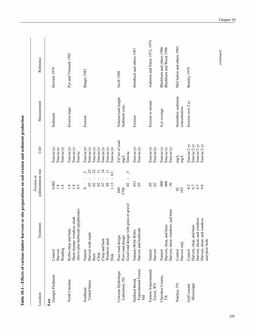
105
Ta
ble
10.1
—E
ffec
ts o
f vari
ou
s ti
mb
er h
arv
ests
or
site
pre
para
tion
s on
soil
ero
sion
an
d s
edim
ent
pro
du
ctio
n
Ero
sio
n o
r
Lo
cati
on
Tre
atm
ent
sed
imen
tati
on
rat
eU
nit
Mea
sure
men
tR
efer
ence
East G
eorg
ia P
ied
mo
nt
Co
ntr
ol
0.0
02
To
ns/
ac/y
rS
edim
ent
Hew
lett
19
79
Har
ves
t1.8
Tons/
ac/y
r
Road
ing
1.6
Tons/
ac/y
r
Nort
h C
aroli
na
Roll
er-c
hop a
nd b
urn
1.8
Tons/
ac/y
rE
rosi
on t
raps
Pye
and V
itouse
k 1
985
Shea
r st
um
ps,
win
dro
w s
lash
1.8
Tons/
ac/y
r
Above
plu
s her
bic
ide
(gly
phosa
te)
4.5
Tons/
ac
So
uth
east
Nat
ura
l0
–.2
To
ns/
ac/y
rE
rosi
on
Bu
rger
19
83
Un
ited
Sta
tes
Har
ves
t w
ith
ro
ads
.05
–.2
3T
ons/
ac/y
r
Burn
.02
–.3
2T
ons/
ac/y
r
Chop
.02
–.1
1T
ons/
ac/y
r
Chop a
nd b
urn
.07
–.1
8T
ons/
ac/y
r
Win
dro
w s
lash
.09
–.1
1T
on
s/ac
/yr
Dis
k1.1
3–
4.5
Tons/
ac/y
r
Co
wee
ta H
yd
rolo
gic
Poor
road
des
ign
840
Yd
3/m
i of
road
Volu
me/
road
len
gth
Sw
ift
1988
Lab
ora
tory
, N
CP
oo
r ro
ad d
esig
n5
70
0m
g/L
Sed
imen
t co
nc.
Good r
oad
des
ign w
ith g
rass
or
gra
vel
.02
–.3
Tons/
ac
Hu
bbar
d B
roo
kN
atu
ral
(WS
4-W
S6
).0
11
Tons/
ac/y
rE
rosi
on
Horn
bec
k a
nd o
ther
s 1987
Ex
per
imen
tal
Fo
rest
,H
arves
t an
d h
erbic
ide
.05
Tons/
ac/y
r
NH
Fer
no
w E
xp
erim
enta
lN
atu
ral
.05
To
ns/
ac/y
rE
rosi
on
to
str
eam
Au
ber
tin
an
d P
atri
c 1
97
2,
19
74
Fore
st, W
VH
arves
t.0
2T
ons/
ac/y
r
Cher
okee
County
,N
atura
l.0
08
Tons/
ac/y
r4-y
r av
erag
eB
lack
burn
and o
ther
s 1986
TX
Har
ves
t, c
ho
p,
and
bu
rn.0
06
Tons/
ac/y
rB
lack
burn
and W
ood 1
990
Har
ves
t, s
hea
r, w
indro
w, an
d b
urn
.36
Tons/
ac/y
r
Nat
chez
, T
NC
ontr
ol
82
mg/L
Sto
rmfl
ow
sed
imen
tM
cClu
rkin
an
d o
ther
s 1
98
5
Har
ves
t o
nly
18
3m
g/L
con
cen
trat
ion
Gu
lf c
oas
tal
Co
ntr
ol
0.2
To
ns/
ac/2
yr
Ero
sio
n o
ver
2 y
rB
easl
ey 1
97
9
Mis
siss
ippi
Har
ves
t, c
hop, an
d b
urn
6.7
Tons/
ac/2
yr
Har
ves
t, s
hea
r, a
nd w
indro
w6.7
Tons/
ac/2
yr
Har
ves
t, s
hea
r, a
nd w
indro
w9.0
Tons/
ac/2
yr
and
plo
w b
eds
con
tin
ued
Chapter 10

106
Timber ManagementT
ab
le 1
0.1
—E
ffec
ts o
f v
ari
ou
s ti
mb
er h
arv
ests
or
site
pre
pa
rati
on
s o
n s
oil
ero
sio
n a
nd
sed
imen
t p
rod
uct
ion
(co
nti
nu
ed)
Ero
sio
n o
r
Lo
cati
on
Tre
atm
ent
sed
imen
tati
on
rat
eU
nit
Mea
sure
men
tR
efer
ence
East
(co
nti
nu
ed)
South
Car
oli
na
Cle
arcu
t.0
7T
ons/
ac/y
rE
rosi
on
Van
Lea
r an
d o
ther
s 1985
Contr
ol
.01
Tons/
ac/y
r
Su
mte
r N
atio
nal
Lo
w-i
nte
nsi
ty b
urn
.06
Tons/
ac/y
rE
rosi
on
Robic
han
d a
nd W
aldro
p 1
994
Fore
st, S
CH
igh-i
nte
nsi
ty b
urn
2.6
Tons/
ac/y
r
Wes
t
Ore
go
nR
oad
s>
.25
In./
yr
Ro
ad s
urf
ace
Fre
dri
kse
n 1
96
5
Fra
ser
Exper
imen
tal
Contr
ol
.018
Tons/
ac/y
rT
o s
trea
mL
eaf
1974
Fo
rest
, C
OR
oad
s an
d h
arv
est—
Fo
ol
Cre
ek.0
05
Tons/
ac/y
rL
eaf
1974
Road
s an
d h
arves
t—D
eadhors
e.0
14
Tons/
ac/y
rS
tott
lem
eyer
1987
H.J
. Andre
ws
Contr
ol
WS
9.0
14
Tons/
ac/y
rT
o s
trea
mS
oll
ins
and o
ther
s 1980
Exper
imen
tal
Cle
arcu
t W
S10
.09
Tons/
ac/y
r
Fore
st, O
R
Ou
ach
ita
Co
ntr
ol
.00
5T
on
s/ac
/yr
Su
rfac
e er
osi
on
Mil
ler
and
oth
ers
19
88
Mounta
ins,
AR
Har
ves
t, r
oll
er-c
hop, an
d b
urn
.09
Tons/
ac/y
r
Har
ves
t, s
elec
tion c
ut
.018
Tons/
ac/y
r
Sil
ver
Cre
ek, ID
Cle
arcu
t w
ith b
uf f
er5.8
Tons/
ac/y
r—1
st y
rE
rosi
on
Cla
yto
n a
nd K
enned
y 1
985
1.8
Tons/
ac/y
r—2
d y
r
Bea
ver
Cre
ek,
Contr
ol
.009
–.0
9T
ons/
ac/y
rA
nnual
ran
ge
War
d a
nd B
aker
1984
AZ
Contr
ol
11
Tons/
ac/y
rO
bse
rved
max
imum
31%
cle
arcu
t1.3
Tons/
ac/y
rO
bse
rved
max
imum
100%
cle
arcu
t27.4
Tons/
ac/y
rO
bse
rved
max
imum
Cle
arcu
t.1
4T
on
s/ac
/yr
Plo
t er
osi
on
Hee
de
and
Kin
g 1
99
0
Cas
par
Cre
ek,
CA
Sel
ecti
ve
clea
rcut
4.5
Yd
3/a
c/y
rE
rosi
on
Kra
mm
es a
nd
Bu
rns
19
73
Dre
w C
ounty
, AR
Cle
arcu
t.1
20
Tons/
ac/y
rE
rosi
on
Bea
sley
and G
ranil
lo 1
988
Sel
ecti
on c
ut
.005
Tons/
ac/y
r
Contr
ol
.002
Tons/
ac/y
r
Cla
rk C
ounty
, AR
Cle
arcu
t—m
echan
ical
pre
p.2
4T
ons/
ac/y
rE
rosi
on
Bea
sley
and o
ther
s 1986
Cle
arcu
t—ch
emic
al p
rep
.11
Tons/
ac/y
r
Contr
ol
.03
Tons/
ac/y
r
Conc.
= c
once
ntr
atio
n, W
S =
wat
ersh
ed.

107
Some form of site preparation is often needed to ensure the
establishment of tree reproduction after timber harvest. The
purpose of site preparation is to provide the environmental
conditions necessary for seed or seedling survival and early
growth. Site preparation usually involves providing a
mineral seedbed and controlling competing and non-
desirable vegetation. Site preparation treatments include
fire, herbicide application, slashing and windrowing, roller
chopping, soil disking, or other mechanical techniques.
Fertilizer may be applied to help establish seedlings and to
speed their growth after establishment.
In the Southeastern United States, upland hardwood stands
are sometimes converted to pine (Pinus spp.). Site prepara-
tion treatments include burning or chemical treatments to
kill the existing vegetation. Soils in the region are often fine
textured and deep and may continue to erode at an acceler-
ated rate for a few years. A winter burn and herbicide
application increased stormflows, overland flows, peak-
flows, and sediment production from two small watersheds
in northern Mississippi (Ursic 1970). Three years after the
fire, when monitoring ended, most of the hydrologic effects
were still evident.
Suspended sediment transport varies with the areal extent of
the soil disturbance, nearness of a stream, and stream
energy. Suspended sediments are often fine-textured
materials with large surface areas per unit of weight. These
large surface areas are reactive and may adsorb and absorb
various constituents including phosphorus, introduced
chemicals, and petroleum products.
Streamside vegetation or filter strips have been used to
prevent overland flow and soil erosion from reaching
surface waters. The filter strip, or equivalent, decreases the
velocity of the overland flow by surface roughness. The
decreased velocity allows sediment to settle out and over-
land waters to infiltrate into the undisturbed soils. The
streamside vegetation filters were originally used to control
or limit road-derived sediment from reaching forest streams.
The filter was a recommended width and was dependent on
hillslope. These filter strips are effective in sediment
removal unless an extreme precipitation or overland flow
event exceeds the sediment detention/retention capacity. The
characteristics that make filter strips work include width,
vegetative and litter cover, surface roughness, and micro-
topography. Microtopography allows overland flow to
concentrate in certain areas and flowpaths. Control of road-
derived sediment migration is frequently by these strips. The
effectiveness of filter strips on controlling soil erosion for
most harvest and site preparation practices has not been
rigorously tested.
Routing and storage are particularly important components
in the transport of sediment through the stream system. They
are critical to the quantification of short- and long-term
impacts of land-use activities on the quality of drinking
water sources. However, the storage and routing processes
are highly variable and do not exhibit steady-state behavior
(see chapter 3).
Catchment studies have identified correlations between
annual peak discharge and annual sediment discharge and
between total annual flow and annual sediment discharge
(NCASI 1999a). Altering flow and erosion may upset
channel stability, increasing turbidity and sediment concen-
trations to drinking water sources.
Reliability and Limitations of Findings
Studies have shown that increased site disturbance has the
potential to increase soil erosion and sediment production.
Soil erosion and sediment yield from undisturbed forest
watersheds are low. Site disturbance from timber harvesting
activities vary by logging and yarding techniques, site
preparation practice, operator techniques, soil vegetative
cover, slope, soil moisture, soil depth, and soil texture
among other environmental factors. Soil erosion processes
are well understood, and models have been developed for
regional predictions of soil erosion throughout the United
States.
Measuring instantaneous sediment concentration (and
turbidity) in small streams is relatively easy. Measuring soil
erosion is not. Erosion is variable in time and space, and the
eroded soil must reach the stream channel to become
sediment. Once in the stream channel, most of the sediment
is transported irregularly when streamflows are high.
Sediments may be stored in the channel and released over a
long period. In-channel disturbances may create in-channel
sediment sources, separate from the hillslope processes.
Large sediment inputs to stream channels can be assessed by
monitoring the physical features of the channel (MacDonald
and others 1991, State of Idaho 1987). Such features include
channel width-to-depth ratios, pool volume occupied by
sediment, and substrate size and particle size distribution.
Research Needs
1. There is no standard or protocol for erosion plot research
on forest land. A standard research method for soil
erosion studies should be decided upon.
2. The importance of dry ravel as an agent of erosion needs
further investigation.
Chapter 10
108
Timber Management
3. Research is needed on routing eroded soil to streams.
Erosion does not equal suspended sediment. Measured
erosion rates do not or should not imply that eroded soil
is reaching the stream channel. Suspended sediment
monitoring is not difficult, but requires labor and equip-
ment that may not be available. For source areas the
question is: Do suspended sediment concentrations best
measure the effects of site disturbance?
4. Recommendation and design of vegetative filter strips are
often based on width only. Research needs to better
define the characteristics that control sediment movement
including slope, vegetative and litter cover, runoff
velocity and volume, surface roughness, and micro-
topography of the filter strip and disturbed area above.
5. Research is needed on monitoring of stream channel
geomorphologic features, which may provide a good
measure of land-use effects, particularly multiple or
cumulative effects. Increased annual water yield from
timber harvesting has been well documented, but the
effect of timber harvesting on peak flows is less clear.
Can this altered hydrology increase sediment transport
from in-channel sources and result in changes in channel
morphology? Conversely, how much increased sediment
input can a stream segment receive without changes in
channel morphology?
Key Points
Site disturbance may result in soil compaction and de-
creased infiltration capacity. If infiltration capacity is
exceeded by precipitation intensity, overland flow may
result in soil erosion and suspended sediment production.
Even undisturbed forest watersheds produce sediment,
mostly from in-channel sources. Sediment impacts from
timber management activities can be minimized by:
1. Careful planning, supervising, and implementing of
forest practices.
2. Keeping the treatment area small and hydrologically
isolated.
3. Leaving adequate filter strips between treatment areas
and streams.
4. Maintaining ground cover in the treatment area to reduce
surface runoff and erosion, and increasing the effective-
ness of filter strips to trap eroded soil before it enters the
stream.
5. Operating during the season with the lowest erosion risk.
Stream Temperature
Issues and Risks
Forest management activities can increase, maintain, or
decrease water temperature. Such changes can affect
drinking water quality (chapter 2) by altering dissolved
oxygen and survival rates of pathogens.
Findings from Studies
Surprisingly few studies have been published on the effects
of silvicultural practices on water temperature, and most of
these were conducted in the 1970’s (table 10.2). These
studies include harvesting with and without streamside
vegetation buffers. Several synthesis papers indicate that
few additional temperature studies have been conducted
(Beschta and others 1987, Binkley and Brown 1993a,
Swank and Johnson 1994).
Exposure of small streams to direct solar radiation is the
dominant process for stream temperature increases
(Tiedemann and others 1988). Other mechanisms including
increased air temperature, channel widening, soil water
temperature increases, and streamflow modification have
been proposed [Ice, in press (a)]. Small streams with smaller
surface areas may be more susceptible to heating, but
usually return to expected temperature within 500 feet [150
meters (m)] downstream [Andrus and Froehlich 1991; Ice,
in press (b)]. Maintaining shade in riparian zones can be
used to avoid most temperature increases in small streams.
As stream width increases, more of the water surface is
exposed to sunlight and the influence of riparian canopy on
stream temperature decreases.
Literature on the effects of timber harvesting on stream
temperatures (table 10.2) shows daily maximum stream
temperature increases from 1.2 to 7.2 oC in eastern forests
and 0.6 to 8 oC in western forests. The range in temperature
increases reflects a range in streamside vegetation buffers
from no buffer to a 100-m buffer. Changes in minimum
nighttime stream temperatures (during the winter or dormant
season) range from no change to < 1 oC in the East and from
zero to < 2 oC in the West.
Reliability and Limitations of Findings
Stream temperatures in small streams may increase after
timber harvesting when the streamside vegetation canopy is
removed. This effect can be mitigated by maintaining
streamside buffers. Several studies have reported tempera-
ture increases with streamside buffers, but increases are
much smaller than for fully exposed streams. The lack of
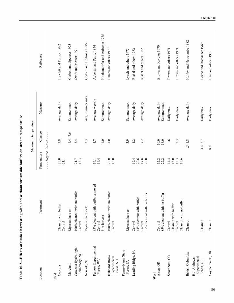
109
Chapter 10T
ab
le 1
0.2
—E
ffec
ts o
f ti
mb
er h
arv
esti
ng
wit
h a
nd
wit
ho
ut
str e
am
sid
e b
uff
ers
on
str
eam
tem
per
atu
re
Max
imum
tem
per
ature
Loca
tion
Tre
atm
ent
Tem
per
ature
Chan
ge
Mea
sure
Ref
eren
ce
- -
- -
Deg
ree
Cel
sius
- -
- -
East G
eorg
iaC
lear
cut
wit
h b
uff
er25.0
3.9
Aver
age
dai
lyH
ewle
tt a
nd F
ort
son 1
982
Contr
ol
21.1
Mar
yla
nd
Rip
aria
n h
arv
est
4.4
–7
.6S
um
mer
max
.C
orb
ett
and
Sp
ence
r 1
97
5
Co
wee
ta H
yd
rolo
gic
100%
cle
arcu
t w
ith n
o b
uff
er21.7
3.4
Aver
age
dai
lyS
wif
t an
d M
esse
r 1971
Lab
ora
tory
, N
CC
ontr
ol
18.3
New
ark, N
JR
ipar
ian h
erbic
ide
3.3
Avg. su
mm
er m
ax.
Co
rbet
t an
d H
eilm
an 1
97
5
Fer
no
w E
xp
erim
enta
l9
5%
cle
arcu
t w
ith
bu
ffer
rem
oved
16.1
1.7
Aver
age
wee
kly
Auber
tin a
nd P
atri
c 1974
Fore
st, W
VC
ontr
ol
14.4
Plo
t har
ves
t4.0
Sum
mer
max
.K
och
endorf
er a
nd A
uber
tin 1
975
Hubbar
d B
rook
100%
cle
arcu
t w
ith n
o b
uff
er20.0
4.0
Aver
age
dai
lyL
iken
s an
d o
ther
s 1970
Ex
per
imen
tal
Co
ntr
ol
16
.0
Fore
st, N
H
Pen
nsy
lvan
ia S
tate
Fo
rest
, PA
Rip
aria
n h
arv
est
3.9
Su
mm
er m
ax.
Ly
nch
an
d o
ther
s 1
97
5
Lea
din
g R
idge,
PA
Contr
ol
19.4
1.2
Aver
age
dai
lyR
ishel
and o
ther
s 1982
44%
cle
arcu
t w
ith b
uff
er20.6
Contr
ol
17.8
7.2
Aver
age
dai
lyR
ishel
and o
ther
s 1982
85%
cle
arcu
t w
ith n
o b
uff
er25.0
Wes
t
Als
ea, O
RC
ontr
ol
12.2
10.0
Aver
age
dai
lyB
row
n a
nd K
rygie
r 1970
85%
cle
arcu
t w
ith n
o b
uff
er22.2
16.0
Sum
mer
max
.
Ste
ambo
at,
OR
Co
ntr
ol
14
.4.6
Dai
ly m
ax.
Bro
wn
an
d o
ther
s 1
97
1
Cle
arcu
t w
ith b
uff
er15.0
Co
ntr
ol
13
.32
.3D
aily
max
.B
row
n a
nd
oth
ers
19
71
Cle
arcu
t w
ith n
o b
uff
er15.6
Bri
tish
Colu
mbia
Cle
arcu
t.5
–1.8
Aver
age
dai
lyH
olt
by a
nd N
ewco
mbe
1982
H.J
. Andre
ws
Ex
per
imen
tal
Fore
st, O
RC
lear
cut
4.4
–6.7
Dai
ly m
ax.
Lev
no a
nd R
oth
acher
1969
Coyote
Cre
ek, O
RC
lear
cut
8.0
Dai
ly m
ax.
Har
r an
d o
ther
s 1
97
9
110
documentation on buffer characteristics makes extrapolation
difficult. Different measurements of stream temperature also
make direct comparisons difficult. Studies have reported
daily, monthly, or seasonal maxima or mean temperatures.
Within-stream temperature variability often is not consid-
ered in monitoring programs.
Attributes needed to estimate the contribution of forest
overstory to stream surface shade include stream width,
distance from vegetation to stream, stream orientation,
height and density of vegetation, crown or canopy measure-
ment, latitude, date, and time (Quigley 1981).
A simpler model developed to predict the effect of
clearcutting on temperatures of small streams uses the
calculated heat load to the stream surface area (Brown
1970). This or similar models should be validated before
use. It would be difficult to suggest one streamwater buffer
model as suitable for all forest watersheds, but measurement
of the angular canopy density can determine the importance
of a buffer strip to prevent stream temperature increases
after timber harvesting. Angular canopy density is the
projection of the streamside vegetation canopy measured at
the angle above the horizon at which direct-beam solar
radiation passes through the canopy (Beschta and others
1987).
Generally, forest practices that open small stream channels
to direct solar radiation are the practices that increase stream
temperatures. Retention of streamside vegetation appears to
mitigate potential temperature changes, especially the
greater temperature changes. These principles are well
documented by research throughout the country. Streamside
canopy removal may also decrease winter streamwater
temperatures, since radiation losses may be increased. For
small streams, temperature returns to undisturbed levels
within a short distance downstream of where canopy shade
is reestablished.
Accurate stream temperature assessments vary from a single
instantaneous measurement to continuous measurement,
depending on the stream diel and seasonal variations.
Stream temperature data need to be evaluated over the long
term. Statistical methods include harmonic analysis, time
series, and trend analysis2 (Hostetler 1991, Limerinos
1978).
Research Needs
1. Stream temperature monitoring and reporting protocols
need to be developed.
2. The range or daily variation in temperature may increase
after removal of streamside vegetation. Research is
needed on these variations because they might affect
drinking water quality.
3. Timber harvesting with proper streamside vegetation
buffers should cause minimal stream temperature
changes. Stream buffers are defined by width only. More
studies need to be conducted investigating the efficiency
of different components of streamside canopy cover on
stream temperatures.
4. Stream temperature monitoring has tended to emphasize
physical measurements of temperature. Remote sensing of
stream temperature may provide more data on tempera-
ture changes over time and space.
5. Few water-quality related studies have assessed cumula-
tive watershed effects. Temperature measurement studies
at different spatial scales need to be conducted. Long-term
temperature data are needed to place the potential effects
of changes in stream temperature in the context of global
or regional cycles of climate change or variability. Long-
term records of stream temperature in undisturbed,
forested watersheds need to be collected.
Key Points
In general, removal of streamside vegetation cover has the
potential to increase streamwater temperatures during the
day in the summer. In certain settings, the vegetation
removal may allow for decreased nighttime temperatures,
especially in the winter. Temperature changes return to
pretreatment levels as the streamside vegetation reestab-
lishes. Streamside vegetation to maintain a thermal cover
over the stream is key to maintaining stream temperatures at
existing levels.
Nutrients
Water from forested watersheds is typically lower in
nutrients than water that drains from other lands. Forest
management activities such as forest cutting and harvesting
may increase annual water yields (Bosch and Hewlett 1982,
Stednick 1996), interrupt the natural cycling of nutrients,
and increase nutrient concentrations in streamwaters.
Nitrogen and phosphorus cycles and their impacts on
drinking water quality are discussed in chapter 2.2 Stednick, J.D. 1999. Stream temperature trends in the New Alseawatershed study. [55 p.]. Unpublished report. On file with: Department of
Earth Resources, Colorado State University, Fort Collins, CO 80523–1482.
Timber Management

111
Issues and Risks
Forest management activities, such as timber harvest and
fertilization, can increase nutrient concentrations in streams.
Findings from Studies
Nitrate nitrogen (NO3-N) concentrations are usually quite
low (0.002 to 1.0 milligrams per liter) in streams draining
undisturbed forest watersheds (Binkley and Brown 1993b).
Concentrations are low because nitrogen is used rapidly by
ecosystem biota and because nitrate formation (nitrification)
is relatively slow in forest soils. Slow rates of organic matter
decomposition, acid soil conditions common in forest
environments, and bacterial allelopathy all decrease rates of
nitrification. Organic matter and anaerobic conditions in
saturated riparian soils allow for denitrification, which is the
reduction of nitrate to nitrogen gas, which may be lost to the
atmosphere.
Throughout the United States, studies in many areas have
found that nutrient losses from silvicultural activities to be
minimal and water quality not degraded (Aubertin and
Patric 1974, Chamberlain and others 1991, Harr and
Fredriksen 1988, Hornbeck and Federer 1975, Martin and
others 1984, McClurkin and others 1987, Pierce and others
1972, Rense and others 1997, Sopper 1975, Swank 1988).
Nutrients contained in the organic matter in trees, litter, and
soils can be affected by various forest management prac-
tices. Cutting vegetation disrupts the processes that regulate
the nutrient cycle and may accelerate dissolved nutrient
leaching and loss via streamflow. Exposing sites to direct
sunlight may increase the rate of nitrogen mineralization.
Nutrients associated with eroded soil particles and sediment
may be lost from the site (Swank 1988). There is usually
minimal opportunity for a buildup of these nutrients in the
stream system after a timber harvest because of the normally
brief period of increased nutrient flux to the stream (Currier
1980). Other nutrients rarely cause water-quality problems,
and this discussion is limited to nitrogen and phosphorus.
Forest management activities such as harvesting or thinning
may interrupt nutrient cycles, and nutrients may be released
(Swank and Johnson 1994). Catchment studies have
produced a large body of information on streamwater
nutrient responses, particularly from clearcutting (table
10.3). Changes in streamwater nutrient concentrations vary
substantially among localities, even within a physiographic
region. In central and Southern Appalachian forests, nitrate-
nitrogen, potassium (K+), and other constituents increased
after harvesting, but the changes were small and did not
affect downstream uses (Swank and others 1989).
Clear-cutting in northern hardwood forests may result in
large increases in concentrations of some nutrients
(Hornbeck and others 1987). Research on catchments has
identified some of the reasons for varied ecosystem response
to disturbance (Swank and Johnson 1994). Swank discusses
the long-term nitrate-nitrogen trends after harvest in chapter
11. In areas that are experiencing nitrogen saturation from
deposition of nitrogen compounds in air pollution, distur-
bances such as forest harvesting can produce increased
nitrate levels in streams and ground water (Fenn and others
1998). See chapter 3 for discussion of nitrogen-saturation
effects.
Soil development factors and forest management strategies
influence the rate of nutrient exports after timber harvesting
(Swank and Johnson 1994). The rotation length, the time
interval between timber harvests, is critical in determining
the sustainability of harvest. Nutrient loss by leaching to
streams is usually minor compared to the nutrient loss by
biomass removal (Clayton and Kennedy 1985, Federer and
others 1989, Johnson and others 1988, Mann and others
1988, Martin and Harr 1989). Nutrient loss differences are
also observed between whole tree, saw log, or bole-only
harvesting.
Phosphorus (P) occurs in several forms in surface water
including the dissolved forms of orthophosphates and
dissolved complex organics and in particulate forms
(organic and inorganic) [Ice, in press (b)]. Phosphorus
sources come from dry deposition (dust), wet deposition,
and geologic weathering. Geology is a key factor in phos-
phorus concentrations from forests. Forest watersheds with
more easily weathered rock, such as sedimentary or volcanic
tuff and breccia, have higher instream concentrations than
watershed with resistant rock, such as intrusive igneous.
Dissolved phosphorus is probably one of the least respon-
sive water-quality constituents to forest management.
Total phosphorus is strongly associated with soil particles or
suspended sediment. Practices that increase or reduce
sediment have similar effects on total phosphorus [Ice, in
press (b)].
In general, nutrient mobility from disturbed forests follows
the order: nitrogen > potassium > calcium and magnesium
> phosphorus. Thus, forest harvesting or other disturbances,
such as fire, will generally produce larger differences in
nitrogen concentrations in streamwater than other constitu-
ents. Possible exceptions are the loss of calcium and
potassium documented in the Northeastern United States
where precipitation inputs had greater acidity from fossil
fuel combustion (Federer and others 1989).
Chapter 10

112
Table 10.3—Effects of clearcutting with and without buffers on mean annual nitrate-nitrogen, ammonium-nitrogen, and
total-phosphorus concentrations
Mean concentration
Location Treatment NO3-N NH
4-N Total Pa Reference
- - - - - - - - - - - - - Milligrams per liter - - - - - - - - - - - - -
EastMarcell Experimental 74% clearcut 0.16 0.55 Verry 1972
Forest, MN Control .12 .41
Hubbard BrookExperimentalForest, NH
WS2 100% cut andherbicide 8.67 – 11.94 .04 – .05 0.002 Likens and others 1970
WS4 33% strip cut .19 – .20WS6 Control .16 – .29 .05 – .09 .001
White Mountain, NHSeven catchments Control .02 – .81 Pierce and others 1972
Clearcut 1.31 – 3.84 .01 – .02Upper Mill Brook Control .23 – .27 .02 – .03 Stuart and Dunshie 1976
Clearcut .23 – .96
Leading Ridge, PALR2 100% clearcut
and herbicide .10 – 8.4 Corbett and others 1975LR1 Control .02 – .04
Fernow ExperimentalForest, WV
WS3 100% clearcut .18 – .49 .14 – .35 .04 – .07 Aubertin and Patric 1972, 1974WS4 Control .10 – .32 .13 – .48 .02 – .04
Coweeta HydrologicLaboratory, NC
WS2 Control .004 .002 .006 Douglass and Swank 1975WS28 100% clearcut .094 .003 .004
West
H.J. Andrews Control .020 – .200 .016 – .032 Fredriksen and others 1975Experimental 100% clearcut .001 – .010 .024 – .039Forest, OR
Bull Run, OR 25% clearcut .002 – .093 .001 – .005 .011 – .032 Fredriksen 1971Control .002 – .013 .002 – .005 .014 – .040
Coyote Creek, OR 100% clearcut .001 – .275 .001 – .018 .062 – .100 Harr and others 1979Control .001 – .005 .001 – .014 .036 – .060 Adams and Stack 1989
Chicken Creek, UT 13% clearcut .025 Johnston 1984Control .008
Alsea, OR 85% clearcut .19 – .44 Brown and others 1973Control 1.18 – 1.21
Priest River, ID Control .20 Snyder and others 1975100% clearcut .18
Fraser Experimental 33% clearcut .06 Stottlemeyer 1987Forest, CO Control .006
Beaver Creek, AZ Control .010 Ryan as cited byClearcut .220 Binkley and Brown 1993b
LR = Leading Ridge; NO3-N = nitrate-nitrogen; NH
4-N = ammonium-nitrogen; total P = total phosphorus; WS = watershed.
a Blank columns represent no data collected.
Timber Management

113
Reliability and Limitations of Findings
Research has documented that timber harvesting may
increase nitrate concentrations in soil water and streams.
This finding is generally accepted without controversy.
Soluble phosphorus concentrations are essentially unaf-
fected by timber harvesting activities. Total phosphorus
concentrations are closely linked to sediment concentra-
tions. Some forest types in the United States have few
studies investigating the influence of forest practices on
water quality. The rather consistent streamwater chemistry
response to timber harvesting allows response extrapolation.
However, an often erroneously cited study as an example of
timber harvesting effects on water quality is an early
Hubbard Brook study (Likens and others 1970). In this
study, vegetation was cut, left onsite, and sprayed with a
general herbicide for 3 years to kill any plant regeneration to
research nutrient cycling processes. Nutrient concentrations,
particularly nitrate, increased significantly. This watershed
treatment was not representative of timber harvest and does
not represent the effects of a typical timber harvest on water
quality.
If vegetation is quickly reestablished, nutrient exports are
short-lived and usually do not represent a threat to water
quality or site productivity. There are a couple of possible
exceptions. Nitrogen deposition can accumulate in forest
soils over time, especially in areas with air-quality concerns
(Riggan and others 1985, Silsbee and Larson 1982). If
timber harvesting occurs in these areas, mobilization of
accumulated soil nitrogen may result in higher nitrate
concentrations and outputs in the streamwater (see
chapter 3).
In the Pacific Northwest, water-quality samples from
streams in forests with nitrogen fixing alder (Alnus spp.)
may have higher nitrate concentrations than streams without
alder (Binkley and Brown 1993b, Miller and Newton 1983).
Since nitrogen is being added to the site by fixation, losses
in site productivity are not a concern, but nitrate concentra-
tions may be high enough to affect downstream uses.
Forest harvesting practices that minimize site disturbance
and quickly establish new stands seem to minimize any
potential water-quality effects. Streamside vegetation
buffers are effective for sediment removal and nutrient
removal.
Research Need
Soil water usually has higher nutrient concentrations than
surface or streamwater. Changes in water chemistry at large
scales (watershed to landscape) need to be evaluated,
especially in the context of multiple land-use activities in
time and space for cumulative watershed effects.
Key Point
Timber harvesting may increase nutrient concentrations
in streams, especially nitrate, but any increase is usually
short-lived. Watershed studies show that nutrient concentra-
tions in soil water may be higher than concentrations in
surface water suggesting that other water dilutes off-site
concentrations.
Fertilizer
Urea fertilizer is highly soluble in water and readily moves
into the forest floor and soil with any appreciable amount of
precipitation. Under normal conditions, urea is rapidly
hydrolyzed (4 to 7 days) to the ammonium ion (NH4-N).
When moisture is limited, urea may be slowly hydrolyzed
on the forest floor. Rather than moving into the soil as
ammonium, the increased soil surface pH favors formation
of ammonia (NH3-N), which is lost by volatilization.
Volatilization losses may be significant. Fertilizer usually is
applied in the spring or fall to take advantage of seasonal
precipitation.
Fertilizers may enter surface water by several routes. Direct
application of chemicals to exposed surface water is the
most significant. Identification of surface water bodies prior
to the application essentially eliminates this entry mode.
When fertilizers are volatilized, ammonia absorption by
surface water is minimal (U.S. Department of Agriculture,
Forest Service 1980).
Issues and Risks
The issues and risks associated with fertilizer application are
essentially the same as described in the Nutrients section,
except if inadvertently applied to streams.
Findings from Studies
The reported effects of forest fertilization on water quality,
particularly nutrient concentrations in streams, are variable3
(reviews by Binkley and Brown 1993b, Binkley and others
1999, Bisson and others 1992, Fredriksen and others 1975).
Nutrient retention by forest soils is excellent. Nutrient
3 Stephens, R. 1975. Effects of forest fertilization in small streams on the
Olympic National Forest, fall 1975. Unpublished report. 40 p. On file with:
USDA Forest Service, Olympia Forestry Sciences Laboratory, 3625 93rd
Avenue, South, Olympia, WA 98512 .
Chapter 10

114
concentrations in surface waters after forest fertilization are
usually low (table 10.4). Exceptions may occur in areas
experiencing nitrogen saturation from air pollution inputs.
For example, Fernow Experimental Forest, WV, a site that
shows signs of nitrogen saturation (Fenn and others 1998),
experienced high streamwater nitrate response to nitrogen
fertilization (table 10.4). Ammonium-nitrogen and phospho-
rus are very reactive with forest soils and are retained on
site. Ammonium-nitrogen concentration may increase in
surface water as a result of direct fertilizer application to
open water. Ammonium-nitrogen concentrations, however,
are rapidly reduced through aquatic organism uptake and
stream sediment sorption. See chapter 3 for discussion of
surface and ground water responses to nitrogen additions in
nitrogen-saturated watersheds.
Table 10.4—Effects of forest fertilization on maximum streamwater ammonium-nitrogen and nitrate-nitrogen
concentrations
Location Treatment NH4-N NO3-N Reference
Lbs/ac - - - Milligrams per liter - - - -
East
Fernow Experimental
Forest, WV 230 0.8 19.8 Aubertin and others 1973
West
Coyote Creek, OR 200 .04 .17 Fredriksen and others 1975
Olympic National
Forest, WA 200 .02– .55 .07–3.85 Stephens 1975a
200 .04 .121 Moore 1975
Entiat Experimental
Forest, WA 48 < .02 .210 Klock 1971
50 .068 Tiedemann and Klock 1973
Mitkof Island, AK 187 .003 2.36 Meehan and others 1975
Siuslaw River, OR 200 .49 7.6 Burrough and Froehlich 1972
Cascade Mountains, OR 200 < .01 < .25 Malueg and others 1972
Lake Chelan, WA 70 .011 .510 Tiedemann 1973
South Umpqua River, OR 200 .048 .177 Moore 1971
Ludwig Creek, WA 178 .004 2.7 Bisson and others 1992
NH4-N = ammonium nitrogen; NO3-N = nitrate nitrogen.a Stephens, R. 1975. Effects of forest fertilization in small streams on the Olympic National Forest, fall 1975. 40 p. Unpublished report. On file
with: Olympic National Forest, 1835 Black Lake Boulevard, SW, Olympia, WA 98512.
Nitrate-nitrogen concentrations measured in surface water
usually peak 2 to 4 days after fertilizer application (U.S
Department of Agriculture, Forest Service 1980). The
magnitude of the peak concentration may depend on the
presence and width of streamside buffers and the density of
small feeders and tributaries to the streams. Peak nitrate-
nitrogen concentrations usually decrease rapidly but may
remain above pretreatment levels for 6 to 8 weeks. Winter
storms may also result in peak nitrate-nitrogen concentra-
tions, but these peaks usually decrease over successive
storms, and concentrations decrease quickly between
storms.
Timber Management

115
Reliability and Limitations of Findings
Relatively few studies have been published on the effect of
forest fertilization on water quality, but results generally are
consistent and suggest that concentrations of ammonium-
nitrogen and phosphorus do not increase after fertilization
(NCASI 1999b). Nitrate-nitrogen concentrations may
increase, but increases are short-lived. Publications re-
viewed here suggest minimal water-quality changes under
most conditions and appear universally applicable.
Streamwater responses to fertilizer application are well
understood and may be extrapolated. An exception to this
generalization may be areas showing signs of nitrogen
saturation. Nitrogen fertilization in these areas may increase
stream nitrate.
Forest fertilization may increase nitrate-nitrogen concentra-
tions by direct application of fertilizer to the stream or by a
runoff-generating precipitation event after application.
Careful delineation of application areas will avoid direct
stream inputs. Fertilizer application timing with respect to
seasonal precipitation or storm events minimizes fertilizer
affects on water quality.
Research Needs
1. Streamside vegetation buffers or management zones are
usually prescribed as a width. We need to know what
specific components or processes in these streamside
areas would minimize the movement of fertilizers into
surface water.
2. Recent research identified certain bedrock materials as
significant sources of nitrogen. Heretofore, geologic
materials were not considered significant sources of
nitrogen. How common are these materials?
3. What are the effects of repeated fertilizer applications in
short-rotation forest plantations on water quality?
4. Response of stream nitrate to fertilization in areas
experiencing nitrogen saturation is poorly understood
and needs more study.
Key Points
Application of nitrogen or phosphorus fertilizers will not
adversely affect surface waters including drinking waters,
when the fertilizer is applied at a rate and time when the
vegetation can use it. Fertilizer application should be timed
to avoid rainy periods if fertilizer might be moved directly
to surface waters. Streamside vegetation is effective in
nutrient removal. Any increase in nutrient concentrations
from fertilizer applications is usually short-lived and should
not affect downstream uses.
Literature Cited
Adams, P.W.; Stack, W.R. 1989. Streamwater quality after logging in
southwest Oregon. Proj. Comp. Rep. Suppl. PNW 87–400. Portland,
OR: U.S. Department of Agriculture, Forest Service, Pacific Northwest
Forest and Range Experiment Station. 28 p.
Andrus, C.W.; Froehlich, H.A. 1991. Riparian forest development after
logging or fire in the Oregon coast range: wildlife habitat and timber
value. In: The New Alsea watershed study. Tech. Bull. 602. New York:
National Council for Air and Stream Improvement. 70 p.
Aubertin, G.M.; Patric, J.H. 1972. Quality water from clearcut forest
land? Northern Logger and Timber Processor. March: 14–15, 22–23.
Aubertin, G.M.; Patric, J.H. 1974. Water quality after clearcutting a small
watershed in West Virginia. Journal of Environmental Quality. 3:
243–249.
Aubertin, G.M.; Smith, D.W.; Patric, J.H. 1973. Quantity and quality of
streamflow after urea fertilization on a forested watershed: first-year
results. In: Forest fertilization symposium proceedings; [Date of meeting
unknown]; [Location of meeting unknown]. Gen. Tech. Rep. NE–3.
Upper Darby, PA: U.S. Department of Agriculture, Forest Service,
Northeastern Forest Experiment Station: 86–100.
Beasley, R.S. 1979. Intensive site preparation and sediment losses on steep
watersheds in the Gulf Coastal Plain. Soil Science Society of America
Journal. 43: 412–417.
Beasley, R.S.; Granillo, A.B. 1988. Sediment and water yields from
managed forests on flat Coastal Plain sites. Water Resources Bulletin.
24(2): 361–366.
Beasley, R.S.; Granillo, A.B.; Zillmer, V. 1986. Sediment losses from
forest management: mechanical vs. chemical site preparation after
clearcutting. Journal of Environmenal Quality. 15(9): 413–416.
Bell, M.A.; Beckett, J.M.; Hubbard, W.F. 1974. Impact of harvesting on
forest environments and resources. Ottawa, Ontario, Canada: Canadian
Forest Service, Environment Canada. 39 p.
Beschta, R.L.; Bilby, R.E.; Brown, G.W. [and others]. 1987. Stream
temperature and aquatic habitat: fisheries and forestry interactions. In:
Salo, E.O.; Cundy, T.W., eds. Streamside management: forestry and
fishery interactions. Seattle: University of Washington: 191–232.
Beschta, Robert L. 1978. Long term patterns of sediment production
following road construction and logging in the Oregon coast range.
Water Resources Research. 14(6): 1011–1016.
Binkley, D.; Brown, T. 1993a. Forest practices as nonpoint sources of
pollution in North America. Water Resources Bulletin. 29(5): 729–740.
Binkley, D.; Brown, T. 1993b. Management impacts on water quality of
forests and rangelands. Gen Tech. Rep. RM–239. Fort Collins, CO: U.S.
Department of Agriculture, Forest Service, Rocky Mountain Forest and
Range Experiment Station. 114 p.
Binkley, D.; Burnham, D.H.; Allen, H.L. 1999. Water quality impacts of
forest fertilization with nitrogen and phosphorus. Forest Ecology and
Management. 121: 191–213.
Chapter 10

116
Bisson, P.A.; Quinn, T.P.; Reeves, G.H.; Gregory, S.V. 1992. Best
management practices, cumulative effects, and long-term trends in fish
abundance in Pacific Northwest river systems. In: Naiman, R., ed.
Watershed management: balancing sustainability and environmental
change. New York: Springer-Verlag: 189–232.
Blackburn, W.H.; Wood, J.C. 1990. Nutrient export in stormflow forest
harvesting and site-preparation in east Texas. Journal of Environmental
Quality. 19: 402–408.
Blackburn, W.H.; Wood, J.C.; DeHaven, M.G. 1986. Stormflow and
sediment losses from site-prepared forest land in east Texas. Water
Resources Research. 22: 776–784.
Bosch, J.M.; Hewlett, J.D. 1982. A review of catchment experiments to
determine the effect of vegetation changes on water yield and evapo-
transpiration. Journal of Hydrology. 55: 3–23.
Brown, G.; Carlson, D.; Carter, G. [and others]. 1976. Meeting water
quality objectives on State and private lands through the Oregon Forest
Practices Act. Corvallis, OR: Oregon State University, Department of
Forestry. 13 p.
Brown, G.W. 1970. Predicting the effect of clearcutting on stream
temperature. Journal of Soil and Water Conservation. 28(1): 11–13.
Brown, G.W.; Gahler, A.R.; Marston, R.B. 1973. Nutrient losses after
cleacut logging and slash burning in the Oregon coast range. Water
Resources Research. 9: 1450–1453.
Brown, G.W.; Krygier, J.T. 1970. Effects of clearcutting on stream
temperatures. Water Resources Research. 6: 1133–1140.
Brown, G.W.; Krygier, J.T. 1971. Clear cut logging and sediment
production in the Oregon coast range. Water Resources Research. 7(5):
1189–1198.
Brown, G.W.; Swank, G.W.; Rothacher, J. 1971. Water temperature in
the steamboat drainage. Res. Pap. PNW–119. Portland, OR: U.S.
Department of Agriculture, Forest Service, Pacific Northwest Forest
Experiment Station. 17 p.
Burger, J.A. 1983. Physical impacts of harvesting and site preparation on
soil. In: Maintaining forest site productivity: Proceedings of the 1st
regional technical conference; [Location of meeting unknown]; [Date of
meeting unknown]. Clemson, SC: Appalachian Society of American
Foresters. 99 p.
Burrough, E.R., Jr.; Froehlich, H.A. 1972. Effects of forest fertilization
on water quality in two small Oregon watersheds. Tech. Note 159.
Portland, OR: U.S. Department of the Interior, Bureau of Land
Management. 8 p.
Chamberlain, T.W.; Harr, R.D.; Everest, F.H. 1991. Timber harvesting,
silviculture, and watershed processes. Influences of forest and rangeland
management on salmonid fishes and their habitats. Spec. Publ. 19.
Bethesda, MD: American Fisheries Society: 181–205.
Clayton, J.L.; Kennedy, D.A. 1985. Nutrient losses from timber harvest in
the Idaho batholith. Soil Science Society of America Journal. 49:
1041–1049.
Corbett, E.S.; Heilman, R.E. 1975. Effects of management practices on
water quantity and quality: New Jersey municipal watersheds. GTR–
NE–13. Upper Darby, PA: U.S. Department of Agriculture, Forest
Service, Northeastern Forest Experiment Station. 196 p.
Corbett, E.S.; Lynch, J.A.; Sopper, W.E. 1975. Forest-management
practices as related to nutrient leaching and water quality. In: Proceed-
ings of a conference on non-point sources of water pollution; 1975 May
1–2; Blacksburg, VA. Blacksburg, VA: Virginia Water Resouces
Research Center: 157–173.
Corbett, E.S.; Spencer, W. 1975. Effects of management practices on
water quantity and quality. GTR–NE–13. Upper Darby, PA: U.S.
Department of Agriculture, Forest Service, Northeastern Forest
Experiment Station: 25–31.
Currier, J.B. 1980. Nutrients. In: An approach to water resources
evaluation of non-point silvicultrual sources (a procedural handbook).
USEPA–600/8/80–012. Washington, DC: U.S. Environmental Protection
Agency. 900 p. Chapter 10.
Davis, M.B. 1976. Pleistocene biography of temperate deciduous forests.
Geoscience Manuscript. 13: 113–126.
Douglass, J.E.; Swank, W.T. 1975. Effects of management practices on
water quality and quantity: Coweeta Hydrologic Laboratory, NC. Gen.
Tech. Rep. NE–13. Upper Darby, PA: U.S. Department of Agriculture,
Forest Service, Northeastern Forest Experiment Station: 1–13.
Dunne, T.; Leopold, L. 1979. Water in environmental planning. San
Francisco: W.H. Freeman and Company. 818 p.
Falletti, D.A. 1977. Sediment production in wildland environments: a
review. In: Soil erosion: prediction and control. Spec. Publ. 21. West
Lafayette, IN: Soil Conservation Society of America. 393 p.
Federer, C.A.; Hornbeck, J.W.; Tritton, L.M. [and others]. 1989. Long-
term depletion of calcium and other nutrients in Eastern U.S. forests.
Environmental Management. 13: 593–601.
Feller, M.C.; Kimmins, J.P. 1984. Effects of clearcutting and slash
burning on streamwater chemistry and watershed nutrient budgets in
southwestern British Columbia. Water Resources Research. 20: 29–40.
Fenn, M.E.; Poth, M.A.; Aber, J.D. [and others]. 1998. Nitrogen excess
in North American ecosystems: predisposing factors, ecosystem
responses, and management strategies. Ecological Applications. 8:
706–733.
Fredriksen, R.L. 1965. Sedimentation after logging road construction in a
small western Oregon watershed. In: Proceedings of the Federal
interagency sediment conference; 1963 January 28–February 1;
Jackson, MS. Misc. Publ. 970. Washington, DC: U.S. Government
Printing Office: 56–59.
Fredriksen, R.L. 1971. Comparative chemical quality—natural and
disturbed streams following logging and slash burning. In: Krygier, J.T.;
Hall, J.D., eds. Symposium on forest land use and the stream environ-
ment; 1970 October 19–21; Corvallis, OR. Corvallis, OR: Oregon State
University Press. 252 p.
Fredriksen, R.L.; Moore, D.G.; Norris, L.A. 1975. Impact of timber
harvest, fertilization, and herbicide treatment on stream water quality in
western Oregon and Washington. In: Bernier, B.; Winget, C.H., eds.
Forest soils and forest land management: Proceedings of the 4th North
American forest soils conference; 1973 August; Quebec, Canada.
Quebec: Laval University Press. 675 p.
Harr, R.D.; Fredriksen, R.L. 1988. Water quality after logging small
watersheds within the Bull Run watershed, Oregon. Water Resources
Bulletin. 24(5): 1103–1111.
Timber Management

117
Harr, R.D.; Fredriksen, R.L.; Rothacher, J. 1979. Changes in streamflow
following timber harvest in southwestern Oregon. Res. Pap. PNW–249.
Portland, OR: U.S. Department of Agriculture, Forest Service, Pacific
Northwest Forest Experiment Station. 22 p.
Heede, B.H.; King, R.M. 1990. State-of-the-art timber harvest in an
Arizona mixed conifer forest has minimal effect on overland flow and
erosion. Hydrological Sciences. 35: 623–635.
Hewlett, J.D. 1979. Forest water quality: an experiment in harvesting and
regenerating Piedmont forest land. Athens, GA: University of Georgia
Printing Office. 28 p. [As cited by Swank, W.T.; DeBano, L.F.; Nelson,
D. 1989. Effects of timber management practices on soil and water. The
scientific basis for silvicultural management decisions in the National
Forest System. In: Burns, R.M., ed. Gen. Tech. Rep. WO-55. Washing-
ton, DC: U.S. Department of Agriculture, Forest Service: 79–106].
Hewlett, J.D.; Fortson, J.C. 1982. Stream temperature under an
inadequate buffer strip in the Southeastern Piedmont. Water Resources
Bulletin. 18(6): 983–988.
Holtby, L.; Newcombe, C.P. 1982. A preliminary analysis of logging
related temperature changes in Carnation Creek, B.C. In: Hartman, G.F.,
ed. Proceedings of the Carnation Creek workshop; [Date of meeting
unknown]; Victoria, BC, Canada: Ministry of Forests and Lands: 81–99.
Hornbeck, J.W.; Federer, C.A. 1975. Effects of management practices on
water quality and quantity: Hubbard Brook Experimental Forest, New
Hampshire. Gen. Tech. Rep. NE–13. Upper Darby, PA: U.S. Department
of Agriculture, Forest Service, Northeastern Forest Experiment Station:
68–75.
Hornbeck, J.W.; Martin, C.W.; Pierce, R.S. [ and others]. 1987. The
northern hardwood forest ecosystem: ten years of recovery from
clearcutting. Res. Pap. NE–RP–596. Broomall, PA: U.S. Department of
Agriculture, Forest Service, Northeastern Forest Experiment Station.
21 p.
Hostetler, S.W. 1991. Analysis and modeling of long term stream
temperatures on the Steamboat Creek Basin, Oregon: implications for
land use and fish habitat. Water Resources Bulletin. 27(4): 637–647.
Ice, G.G. [In press (a)]. Stream temperature and dissolved oxygen: the
Alsea watershed study. In: Stednick, J.D.; ed. The Alsea watershed:
hydrological and biological responses to temperate coniferous forest
practices. New York: Springer-Verlag.
Ice, G.G. [In press (b)]. Streamflow and water quality: what does the
science show about clearcutting in western Oregon. In: Proceedings of a
symposium: clearcutting in western Oregon: what does science show?
1999 November 3; Corvallis, OR. Corvallis, OR: Oregon State
University.
Johnson, D.W.; Kelly, J.M.; Swank, W.T. [and others]. 1988. The effects
of leaching and whole tree harvest on cation budgets of several forests.
Journal of Environmental Quality. 17(3): 418–424.
Johnston, R.S. 1984. Effect of small aspen clearcuts on water yield and
water quality. Res. Pap. INT–333. Ogden, UT: U.S. Department of
Agriculture, Forest Service, Intermountain Research Station. 9 p.
Klock, G.O. 1971. Streamflow nitrogen loss following forest erosion
control fertilization. Res. Note PNW–169. Portland, OR: U.S. Depart-
ment of Agriculture, Forest Service, Pacific Northwest Forest and Range
Experiment Station. 9 p.
Kochenderfer, J.N.; Aubertin, G.M. 1975. Effects of mangement
practices on water quality and quantity: Fernow Experimental Forest,
West Virginia. GTR–NE–13. Upper Darby, PA: U.S. Department of
Agriculture, Forest Service, Northeastern Forest Experiment Station:
14–24.
Krammes, J.S.; Burns, D.M. 1973. Road construction on Caspar Creek
watersheds—10-year report on impact. Res. Pap. PSW–03. Berkeley,
CA: U.S. Department of Agriculture, Forest Service, Pacific Southwest
Forest and Range Experiment Station. 10 p.
Leaf, Charles F. 1974. A model for predicting erosion and sediment yield
from secondary forest road construction. Res. Note RM–274. Fort
Collins, CO: U.S. Department of Agriculture, Forest Service, Rocky
Mountain Forest and Range Experiment Station. 4 p.
Levno, A.; Rothacher, J. 1969. Increases in maximum stream temperature
of the slash burning in a small experimental watershed. Res. Note PNW–
16. Portland, OR: U.S. Department of Agriculture, Forest Service,
Pacific Northwest Forest Experiment Station. 13 p.
Likens, G.E.; Bormann, F.H.; Johnson, N.M. [and others]. 1970. Effects
of forest cutting and herbicide treatment on nutrient budgets in the
Hubbard Brook watershed ecosystem. Ecological Monograph. 40(1):
23–47.
Limerinos, J.T. 1978. Evaluation of thermograph data for California
streams. U.S. Geol. Surv. Water Resour. Invest. 78–66. Menlo Park, CA:
U.S. Geological Survey. 28 p.
Lynch, J.A.; Sopper, W.E.; Corbett, E.S.; Amard, D.W. 1975. Effects of
management practices on water quantity and quality: the Penn State
experimental watersheds. Gen. Tech. Rep. NE–13. Upper Darby, PA:
U.S. Department of Agriculture, Forest Service, Northeastern Forest
Experiment Station: 32–46.
MacDonald, L.; Smart, A.W.; Wissmar, R.C. 1991. Monitoring
guidelines to evaluate the effects of forestry practices on streams in the
Pacific Northwest and Alaska. USEPA/910/9–91–001. Seattle: U.S.
Environmental Protection Agency. 166 p.
Malueg, K.W.; Powers, C.F.; Krawczyk, D.F. 1972. Effects of aerial
forest fertilization with urea pellets on nitrogen levels in a mountain
stream. Northwest Science. 46(1): 52–58.
Mann, L.K.; Johnson, D.W.; West, D.C. [and others]. 1988. Effects of
whole -tree and stem only clearcutting on post harvest hydrologic losses,
nutrient capital and regrowth. Forest Science. 34: 412–428.
Martin, C.W.; Harr, R.D. 1989. Logging of mature Douglas-fir in western
Oregon has little effect on nutrient output budgets. Canadian Journal of
Forest Research. 19: 35–43.
Martin, C.W.; Noel, D.S.; Federer, C.A. 1984. Effects of forest
clearcutting in New England on stream chemistry. Journal of Environ-
mental Quality. 13: 204–210.
McClurkin, D.C.; Duffy, P.D.; Ursic, S.J.; Nelson, N.S. 1985. Water
quality effects of clearcutting Upper Coastal Plain loblolly pine
plantations. Journal of Environmental Quality. 14: 329–332.
McClurkin, D.C.; Duffy, P.D.; Ursic, S.J.; Nelson, N.S. 1987. Changes
in forest floor and water quality following thinning and clearcutting of
20-year-old pine. Journal of Environmental Quality. 16: 237–241.
Chapter 10
118
Meehan, W.R.; Lotspeich, F.B.; Muelle, E.W. 1975. Effects of forest
fertilization in two southeast Alaska streams. Journal of Environmental
Quality. 4(1): 50–53.
Megahan, Walter F. 1975. Sedimentation in relation to logging activities
in the mountains of central Idaho. In: Present and prospective technol-
ogy for predicting sediment yields and sources. Agric. Res. Serv. Rep.
ARS–40. Beltsville, MD: U.S. Department of Agriculture, Agricultural
Research Service: 74–82.9
Miller, E.L.; Beasley, R.S.; Lawson, E.R. 1988. Forest harvest and site
preparation effects on erosion and sedimentation in the Ouachita
Mountains. Journal of Environmental Quality. 17: 219–225.
Miller, J.H.; Newton, M. 1983. Nutrient losses from disturbed forest
watersheds in Oregon’s coast range. Agro-Ecosystems. 8: 153–167.
Moore, D.G. 1971. Fertilization and water quality. In: Proceedings of the
annual meeting of the western reforestation coordination committee;
[Date of meeting unknown]; [Location of meeting unknown]. Portland,
OR: Western Forestry and Conservation Associates: 28–35.
Moore, D.G. 1975. Effects of forest fertilization with urea on water quality
—Quilcene Ranger District, Washington. Res. Note PNW–241. Portland,
OR: U.S. Department of Agriculture, Forest Service, Pacific Northwest
Forest and Range Experiment Station. 9 p.
NCASI. 1999a. Scale considerations and the detectability of sedimentary
cumulative watershed effects. NCASI Tech. Bull. 776. New York:
National Council for Air and Stream Improvement. 227 p.
NCASI. 1999b. Water quality effects of forest fertilization. NCASI Tech.
Bull. 782. New York: National Council for Air and Stream Improvement.
53 p.
Patric, J.H.; Evans, J.O.; Helvey, J.D. 1984. Summary of sediment yield
data from forested land in the United States. Journal of Forestry. 82:
101–104.
Pierce, R.S.; Martin, C.W.; Reeves, C.C. [and others], eds. 1972.
Nutrient losses from clearcuttings in New Hampshire. In: National
symposium on watersheds in transition. 1972 June 19–22; Fort Collins,
CO. Am. Water Resour. Assoc. Proc. Ser. 14. Urbana, IL: American
Water Resources Association: 285–295.
Pye, J.; Vitousek, P. 1985. Soil and nutrient removals by erosion and
windrowing at a Southeastern U.S. Piedmont site. Forest Ecology and
Management. 11: 145–155.
Quigley, T.M. 1981. Estimating contribution of overstory vegetation to
stream surface shade. Wildlife Society Bulletin. 9(1): 22–27.
Renfro, G.W. 1975. Use of erosion equations and sediment delivery ratios
for predicting sediment yield. In: Present and prospective technology for
predicting sediment yields and sources. Agric. Res. Serv. Rep. ARS–40.
Beltsville, MD: U.S. Department of Agriculture, Agricultural Research
Service: 33–45.
Rense, J.D.; Stottlemeyer, R.; Troendle, C.A. 1997. Effect of clearcutting
on nutrient fluxes in a subalpine forest at Fraser, Colorado. Hydrology
and Earth System Sciences. 1(2): 333–344.
Riggan, P.J.; Lockwood, R.N.; Lopez, E.N. 1985. Deposition and
processing of airborne nitrogen pollutants in Mediterranean-type
ecosystems of southern California. Environmental Science and
Technology. 19: 781–789.
Rishel, G.B.; Lynch, J.A.; Corbett, E.S. 1982. Seasonal stream
temperature changes following forest harvest. Journal of Environmental
Quality. 11: 112–116.
Robichand, P.R.; Waldrop, T.A. 1994. A comparison of surface runoff
and sediment yields from low- and high-severity site preparation burns.
Water Resoures Bulletin. 30(1): 27–34.
Rothwell, R.L. 1971. Watershed management guidelines for logging and
road construction. Ottawa, Ontario, Canada: Canadian Forest Service,
Forest Res. Lab. [22 p.].
Silsbee, D.; Larson, G. 1982. Water quality of streams in the Great Smoky
Mountain National Park. Hydrobiologia. 89: 97–115.
Snyder, G.G.; Haupt, H.F.; Belt, G.H., Jr. 1975. Clearcutting and buring
slash alter quality of stream water in northern Idaho. Res. Pap. INT–168.
Ogden, UT: U.S. Department of Agriculture, Forest Service, Intermoun-
tain Forest and Range Experiment Station. 34 p.
Sollins, P.; Grier, C.C.; McCorison, F.M. [and others]. 1980. The
internal element cycles of an old growth Douglas fir ecosystem in
western Oregon. Ecological Monographs. 50: 261–285.
Sopper, W.E. 1975. Effects of timber harvesting and related management
practices on water quality in forested watersheds. Journal of Environ-
mental Quality. 4(1): 24–29.
State of Idaho, Department of Health and Welfare. 1987. State of Idaho
forest practices water quality management plan. Water Qual. Rep. Boise,
ID: Idaho Department of Health and Welfare. 134 p.
Stednick, J.D. 1987. Potential for subalpine forest management practices
on sediment production. In: Management of subalpine forests: building
on 50 years of research. Gen. Tech. Rep. 149. Fort Collins, CO: U.S.
Department of Agriculture, Forest Service, Rocky Mountain Forest
Experiment Station: 95–100.
Stednick, J.D. 1991. Wildland water quality sampling and analysis. San
Diego, CA: Academic Press. 217 p.
Stednick, J.D. 1996. Monitoring the effects of timber harvest on annual
water yield. Journal of Hydrology. 176: 79–95.
Stone, E. 1973. The impact of timber harvest on soils and water. Report of
the President’s Advisory Panel on timber and the environment.
Washington, DC: U.S. Government Printing Office: 427–467.
Stottlemeyer, R. 1987. Natural and anthropic factors as determinants of
long-term stream water chemistry. In: Troendle, C.A.; Kaufmann, M.R.;
Hamre, R.H.; Winokur, R.P., eds. Management of subalpine forests:
building on 50 years of research. Gen. Tech. Rep. RM–149. Fort Collins,
CO: U.S. Department of Agriculture, Forest Service, Rocky Mountain
Forest Experiment Station: 86–94.
Stuart, G.; Dunshie, D. 1976. Effects of timber harvest on water
chemistry. Hydrol. Pap. [Milwaukee, WI]: U.S. Department of
Agriculture, Forest Service, Eastern Region. 34 p.
Swank, W.T. 1988. Stream chemistry responses to disturbance. In: Swank,
W.T.; Crossley, D.A., eds. Forest hydrology and ecology at Coweeta.
New York: Springer-Verlag: 339–358.
Timber Management

119
Swank, W.T.; DeBano, L.F.; Nelson, D. 1989. Effects of timber
management practices on soil and water. In: Burns, R.L., tech. comp.
The scientific basis for silvicultural and management decisions in the
National Forest System. Gen. Tech. Rep. WO–55. Washington, DC: U.S.
Department of Agriculture, Forest Service. 180 p.
Swank, W.T.; Johnson, C.E. 1994. Small catchment research in the
evaluation and development of forest management practices. In:
Biogeochemistry of small catchments: a tool for environmental research.
SCOPE. New York: John Wiley. 419 p. Chapter 17.
Swift, F.W., Jr.; Messer, J.B. 1971. Forest cuttings raise temperatures of
small streams in the Southern Appalachians. Journal of Soil and Water
Conservation. 26: 11–116.
Swift, L., Jr. 1988. Forest access roads: design, maintenance, and soil loss.
In: Swank, W.T.; Crossley, D.A., eds. Forest hydrology and ecology at
Coweeta. New York: Springer-Verlag: 325–338.
Tiedemann, A.R. 1973. Stream chemistry following a forest fire and urea
fertilization in north central Washington. Res. Note PNW–203. Portland,
OR: U.S. Department of Agriculture, Forest Service, Pacific Northwest
Forest and Range Experiment Station. 20 p.
Tiedemann, A.R.; Klock, G.O. 1973. First-year vegetation after fire,
reseeding, and fertilization on the Entiat Experimental Forest. Note
PNW–195. Portland, OR: U.S. Department of Agriculture, Forest
Service, Pacific Northwest Forest and Range Experiment Station. 6 p.
Tiedemann, A.R.; Quigley, T.M.; Anderson, T.D. 1988. Effects of timber
harvest on stream chemistry and dissolved nutrient losses in northeast
Oregon. Forest Science. 2: 344–358.
Ursic, S.J. 1970. Hydrologic effects of prescribed burning and deadening
upland hardwoods in northern Mississippi. Res. Pap. SO–54. New
Orleans: U.S. Department of Agriculture, Forest Service, Southern
Forest Experiment Station. 15 p.
U.S. Department of Agriculture, Forest Service. 1980. An approach to
water resources evaluation of nonpoint silvicultural sources (WRENS).
EPA–600/8–80–012. Springfield, VA: U.S. Environmental Protection
Agency. 900 p.
Van Lear, D.H.; Douglass, J.E.; Cox, S.K.; Augspurger, M.K. 1985.
Sediment and nutrient export in runoff from burned and harvested pine
watersheds in the South Carolina Piedmont. Journal of Environmental
Quality. 14(2): 169–174.
Verry, E.S. 1972. Effect of aspen clearcutting on water yield and quality in
northern Minnesota. In: Csallany, S.D.; McLaughlin, T.G.; Striffler,
W.D., eds. National symposium on watersheds in transition; 1972 June
19–22; Fort Collins, CO. Urbana, IL: American Water Resources
Association: 276–284.
Ward, T.J.; Baker, M.B. 1984. Sediment from managed pine watershed in
northern Arizona. In: Proceedings of the specialty conference of the
irrigation and drainage division of the American society of civil
engineers; [Date of meeting unknown]; Flagstaff, AZ. Flagstaff, AZ:
American Society of Civil Engineers: 552–557.
Chapter 10

120
Chapter 11
Forest Succession
Wayne Swank1
Introduction
The effects of forest management activities on water quality
are generally of the greatest magnitude in the first several
years after disturbance. However, during long-term succes-
sion and regrowth of forest ecosystems, changes in physical,
chemical, and biological parameters of streams may occur.
Nutrients
Issues and Risks
After a forest disturbance such as harvesting or fire, nutrient
levels in streams may be elevated during early successional
stages until the forest matures (see chapter 10). Nitrate
concentrations can be elevated for a few to many years
depending upon whether the watershed is nitrogen limited
or saturated (see chapter 3 for discussion of nitrogen
saturation).
Findings from Studies
Changes in stream inorganic chemistry and sediment yield
were observed over a 20-year period after clearcutting by
cable logging of a 146-acre [58-hectare (ha)] Southern
Appalachian watershed (Swank and others, in press). Stream
nutrient concentrations and fluxes showed small increases
after harvest, and responses were largest the third year after
treatment. Nitrate-nitrogen (NO3
-1) was an exception. The
initial increase in nitrate was from < 0.1 milligrams (mg) per
liter to 0.8 mg per liter (fig. 11.1) and increased net nitrogen
export of 1.16 pounds per acre [1.3 kilograms (kg) per
hectare] the third year after harvest. However, later in
succession (15 to 20 years), nitrate concentrations exceeded
values observed the first several years after clearcutting.
This response is partially attributed to reduction in nitrate
uptake due to vegetation mortality, changes in species
composition, and nitrogen release from decomposition of
woody plants.
Other long-term research in eastern forested watersheds
(Edwards and Helvey 1991, Swank and Vose 1997) shows
that as forests mature, less nitrogen is retained in the
watershed and stream nitrate concentrations increase. These
long-term studies support findings of shorter term stream
chemistry surveys. A survey of streamwater chemistry in 57
watersheds along successional and elevational gradients was
conducted in the White Mountains of New Hampshire
(Vitousek 1977). Differences in successional status among
watersheds were found to be important in controlling nitrate
and potassium concentration. Streams draining old-aged
forests had higher concentrations of nitrate, potassium, and
other solutes than did streams draining intermediate-aged
forests at the same elevation. Spruce-fir (Picea spp.-Abies
spp.) watersheds with no record of logging had streamwater
nitrate concentrations of about 3 mg per liter, while spruce-
fir watersheds logged 30 years previously had nitrate
concentrations < 0.5 mg per liter.
Another survey of 38 streams draining partially or entirely
clearcut watersheds was conducted in New England—
(Martin and others 1985) on northern hardwood sites in
New Hampshire, Maine, and Vermont; in central hardwood
forests in Connecticut; and in coniferous forests in Maine
and Vermont. Streams draining watersheds that had been
partially or entirely clearcut in the previous 2 years were
selected. There were no apparent changes in stream nutrient
concentrations from many of the ecosystems, and the largest
concentration increases were for nitrate, calcium, and
potassium in northern hardwoods of New Hampshire.
Inorganic nitrogen (nitrate plus ammonium) increased to an
average of 2 mg per liter (Martin and others 1985). How-
ever, elevated solute concentrations appear to be short-lived,
even in streams draining successional northern hardwood
forests in New Hampshire (Hornbeck and others 1987).
Moreover, early stream chemistry changes after clearcutting
were considered insufficient to cause concern for public
water supplies or for downstream nutrient loading (Martin
and others 1985).
In the Pacific Northwest, forest-successional stage is not
always a good predictor of nitrate concentration in
streamwater. For example, at the H.J. Andrews Experimen-
tal Forest in Oregon, forest harvest increased annual nitrate1 Retired Project Leader, USDA Forest Service, Southern Research Station,Otto, NC.

121
concentration from predisturbance levels of 0.001 mg per
liter to 0.036 mg per liter (Martin and Harr 1989), but nitrate
concentration returned to predisturbance levels within 6
years. Further, a 20-year postdisturbance record from a pair
of treated and untreated watersheds at the experimental
forest suggests that nitrate concentrations in streamwater
remain very low in both watersheds once the clearcut
watershed recovers from the immediate effects of distur-
bance.2 At the H.J. Andrews Experimental Forest, the
ecosystem is highly nitrogen-limited, and vegetation imprint
on nitrogen fluxes may be overridden by rapid immobiliza-
tion of any available nitrogen by soil microbiota.
An extensive synoptic water-quality assessment was
conducted on numerous streams in the Great Smoky
Mountain National Park in the Southern Appalachian
Mountains (Flum and Nodvin 1995, Silsbee and Larson
1982). Concentrations of nitrate in streams draining water-
sheds that had been logged prior to park establishment were
significantly lower (one-half) than the nitrate concentrations
in unlogged watersheds at similar elevations.
The magnitude of stream nitrate concentrations associated
with long-term forest succession depends on a number of
factors, such as levels of atmospheric nitrogen deposition,
the type and rapidity of forest regrowth, soil microbial
activity, and soil physiochemical reactions. Stream nitrate
levels rarely exceed 5 mg per liter and are below current
drinking water standards. The nitrate, however, may
contribute to stream acidification, particularly during spring
snowmelt when nitrate concentrations peak in the Northeast-
ern United States (Murdock and Stoddard 1992).
Reliability and Limitations of Findings
Existing evidence for changes in stream chemistry with
forest succession is based upon well-established programs
of long-term research and is quite reliable. However,
findings are limited in scope to select forest ecosystems in
the United States.
Limited evidence indicates that stream nitrate concentrations
for older hardwood forests of the southern and central
Appalachian regions are higher than for younger succes-
sional forests. However, site-specific research shows that
nitrate levels can vary substantially even during early
succession (first 20 years), although the general applicability
of findings is unknown. Assessments of nitrate levels in
streams draining successional forests in New England show
mixed responses and appear to be ecosystem specific. Very
limited information on stream nitrate is available for suc-
cessional forests in the Pacific Northwest. Current findings
2 Personal communication. 1999. Kristin Vanderbilt, Graduate Student.Oregon State University, Corvallis, OR.
WS 2
WS 7
1.00
.90
.75
.60
.45
.30
.15
01975 1980 19901985 1995
Year
Road c
onstr
uction
Road s
eedin
g a
nd fert
ilization
Cuttin
g a
nd loggin
g
Site p
repara
tion
Str
eam
NO
3-1
concentr
ation (
mg/L
)
Figure 11.1—Mean monthly concentrations (flow weighted) of nitrate (NO3
-1) in streamwater of a clearcut, cable-logged,
hardwood-covered watershed (WS7) and an adjacent watershed (WS2) during calibration, treatment activities, and
postharvest period, Coweeta Hydrologic Laboratory, North Carolina.
Chapter 11

122
indicate that elevated nitrate concentrations following clear-
cutting are short-lived and return to predisturbance levels
early in succession.
Research Needs
1. Long-term assessments of stream chemistry changes
associated with forest succession are lacking for most
major forest ecosystems in the United States. From a
public drinking water perspective, synoptic stream
nutrient surveys across a range of forest types and stand
ages with known disturbance histories would greatly
enhance planning information for managers.
2. There is a large knowledge gap in nutrient concentration
changes associated with storm runoff events. Such
information is most important where water supplies are
derived from forested headwaters with rapid streamflow
responses to precipitation, e.g., watersheds with shallow
soils, steep slopes, intense rainfall, and rapid snowmelt.
Sediment
Issues and Risks
Stream sediment may also exhibit long-term dynamics after
forest disturbance. Logging roads associated with harvesting
activities are frequently the major source of sediment to
streams and are a potential legacy to consider when evaluat-
ing sources of sediment in drinking water (see chapters 3, 9).
Findings from Studies
A synthesis of long-term sediment yield responses following
forest watershed disturbances is provided by Bunte and
MacDonald (1999). Based on studies in Oregon and New
Hampshire, they identify three kinds of potential responses
in postdisturbance sediment yields:
1. Sediment yields remain high for a number of years after
disturbance due to a large sediment pulse to the stream from
a storm or other disturbance. That is, sediment from up-
stream storage areas or destabilized hillslopes and chan-
nels continues to be released;
2. Sediment yields decline below average annual yields
after disturbance when sediment storage is depleted by a
major sediment transport event; and
3. Sediment yields rapidly return to predisturbance condi-
tions because excess material has moved through the
system.
Recent findings in the Southern Appalachians provide an
example of the first type of response where sediment yield
remains high for a number of years during forest succession
(Swank and others, in press). A cable-logged, clearcut
watershed required only three contour access roads because
logs could be yarded 1,000 feet (305 meters) with the cable
system. Record storms (15 inches or 38 centimeters) in the
last 2 weeks of May 1976, prior to grass establishment,
eroded both unstable soil and hydroseeded materials from
the roads. Roads were the source of elevated sediment yield
as illustrated by soil loss measured at a gaging station in the
stream immediately below a road crossing in the middle of
the catchment (fig.11.2A). In those 2 weeks of May,
sediment yield was nearly 55 tons [50 metric tonnes (Mg)]
from 0.21 acre (0.085 ha) of road contributing area (road-
bed, cut, and fill). In the ensuing period of road stabilization
and minimum use (June to December 1976), soil loss was
low but accelerated again briefly during the peak of logging
activities (fig. 11.2A). In the next year, soil loss below the
road declined to baseline levels.
The pattern of sediment yield at the base of the second-order
stream (fig. 11.2B, gaging site) draining the watershed was
different from the pattern of sediment loss from the roads.
Following an initial pulse of sediment export from the
watershed, sediment yield remained substantially elevated
during and after logging. In the 3-year period between
1977–80, the cumulative increase in sediment yield was 240
tons (218 Mg) (fig. 11.2B). During the next 10 years,
sediment yield declined with a cumulative increase in export
of 240 tons (218 Mg). The rate of sediment yield over the 5-
to 15-year period after disturbance was about 300 lb per acre
per year (336 kg per hectare per year), or 50 percent above
pretreatment levels. The long-term sediment yield data
illustrate a lag or delay between pulsed sediment inputs to a
stream and the routing of sediments through the stream
channels. In the absence of significant additional sources of
sediment to streams on the watershed, annual sediment yield
at the base of the watershed was still substantially above
predisturbance levels at least 15 years later. Thus, there
appears to be a continual release of sediment from upstream
storage that was primarily deposited from road crossings of
streams during exceptionally severe storms.
Reliability and Limitations of Findings
Few studies have documented the long-term effects of
management practices on sediment yield. As pointed out in
chapter 10, increases in sediment yields from timber
management activities are typically considered to be short-
lived. However, unique conditions during management can
lead to elevated stream sediment later in forest succession.
The importance of this process is site-specific and requires
Forest Succession

123
Cum
ula
tive s
edim
ent yie
ld(t
ons)
1975
0
1977 1979 1981 1983 1985 1987 1989
100
200
300
400
500
600
700
Date
(B)
Measured
Predicted
that each stream be evaluated to assess the legacy of past
management practices on current levels of stream
sedimentation.
Research Need
Recommendations for future research related to this topic
are given in chapter 10.
Key Points
In the long term, forest harvesting practices alone may have
little deleterious impact on stream sediment and chemistry,
which are of primary concern in drinking water. However,
other past and present land uses affect present sediment and
nitrate concentrations in streams. Sediment and nitrate
yields associated with early successional development of
forest may be in addition to yields from other past and
present land uses. It is important to consider successional
impacts along with the cumulative impacts of other past and
present land uses across the landscape when assessing
impacts of land management on drinking water sources.
Literature Cited
Bunte, K.; MacDonald, L.H. 1999. Scale considerations and the
detectability of sedimentary cumulative watershed effects. Tech. Bull.
776. Research Triangle Park, NC: National Council for Air and Stream
Improvement. 327 p.
Edwards, P.J.; Helvey, J.D. 1991. Long-term ionic increases from a
control Appalachian forested watershed. Journal of Environmental
Quality. 20: 250–255.
Flum, T.; Nodvin, S.C. 1995. Factors affecting streamwater chemistry in
the Great Smoky Mountains, U.S.A. Water, Air and Soil Pollution. 85:
1707–1712.
Hornbeck, J.W.; Martin, C.W.; Pierce, R.S. [and others]. 1987. The
northern hardwood forest ecosystem: ten years of recovery from
clearcutting. Res. Pap. NE–596. Broomall, PA: U.S. Department of
Agriculture, Forest Service, Northeastern Forest Experiment Station.
30 p.
Martin, C.W.; Harr, R.D. 1989. Logging of mature Douglas-fir in western
Oregon has little effect on nutrient output budgets. Canadian Journal of
Forest Research. 19: 35–43.
Martin, C.W.; Noel, D.S.; Federer, C.A. 1985. Clearcutting and the
biogeochemistry of streamwater in New England. Journal of Forestry.
83(11): 686–689.
Murdock, P.S.; Stoddard, J.L. 1992. The role of nitrate in the acidifica-
tion of streams in the Catskill Mountains of New York. Water Resources
Research. 28(10): 2707–2720.
Silsbee, D.G.; Larson, G.L. 1982. Water quality of streams in the Great
Smoky Mountains National Park. Hydrobiologia. 89: 97–115.
Swank, W.T.; Vose, J.M. 1997. Long-term nitrogen dynamics of Coweeta
forested watersheds in the Southeastern United States of America.
Global Biogeochemical Cycles. 11(4): 657–671.
Swank, W.T.; Vose, J.M.; Elliott, K.J. [In press]. Long-term hydrologic
and water quality responses following commercial clearcutting of mixed
hardwoods on a Southern Appalachian catchment. Forest Ecology and
Management.
Vitousek, P.M. 1977. The regulation of element concentrations in
mountain streams in the Northeastern United States. Ecological
Monographs. 47: 65–87.
Figure 11.2—Cumulative sediment yield measured on a clearcut, cable-
logged, hardwood-covered watershed: (A) in one of the first-order streams
below a logging road during the first 32 months after treatment and (B) in
the ponding basin of the second-order stream at the gaging site during 15
years after treatment. Predicted values are based on pretreatment calibration
of sediment yield with an adjacent control watershed, Coweeta Hydrologic
Laboratory, North Carolina.
Apr NovJuly Apr NovJuly Apr NovJuly
1976 1977 1978
Logging activitiesR
oad c
onstr
uction
Cu
mu
lative
se
dim
en
t yie
ld(t
on
s)
(A)65
50
40
30
20
0
Two major storm events
Chapter 11

124
Chapter 12
Fire Management
Johanna D. Landsberg and Arthur R. Tiedemann1
Introduction
The effect of wildfire on drinking water was graphically
demonstrated when the Buffalo Creek fire in Colorado in
1996 was followed by heavy rains, forcing municipal water
supplies to shut off, one of Denver’s water treatment plants
to close, months to be spent cleaning a water-supply
reservoir, and the Coors Brewing Company to bring in water
by truck (Illg and Illg 1997).
Fire, both wild and prescribed, has the potential to alter
physical, chemical, and biological properties of surface
water that originates from burned wildland areas. Nonpoint-
source pollution from wildland after fire can impair the
suitability of water for drinking and other purposes. New
plans for widespread use of prescribed fire to solve forest
health problems create an urgent need to fully understand
the water-quality consequences of increasing the occurrence
of fire. Fire management activities (like retardant applica-
tion, fireline construction, and postfire rehabilitation) also
have potential effects on water quality.
The most important effects of fire on drinking water source
quality include sediment and turbidity or both, water
temperature, and increased nutrients in streamflow. In this
chapter, we review results of research on the response of the
above water-quality variables to fire, fire management
activities, and fire rehabilitation measures. Much of the
information comes from reports on wildfires. We would
expect the magnitude of streamwater-quality changes after
prescribed fire to be less than those observed after wildfires
and some broadcast slash burns. It is unlikely that prescribed
fire would consume as much forest floor and understory, or
kill as much overstory, as would a wildfire because pre-
scribed fires are usually conducted under conditions
deliberately chosen to produce burns of low severity.
Sediment and Turbidity
Issues and Risks
Suspended sediment is the major nonpoint-source pollution
problem in forests (Society of American Foresters 1995).
Beschta (1990) reported that sediment and turbidity are the
most significant water-quality responses associated with
fire. Turbidity has no direct health effects but can interfere
with disinfection and provides a medium for microbial
growth. Thus, it may indicate the presence of microbes (U.S.
EPA 1999). See chapter 2 for more discussion on the effects
of sediment on drinking water.
Findings from Studies
To understand research findings about sediment production
and its impacts, one must be familiar with the units of
measurement in which sediment is reported. Suspended
sediment is particles carried in suspension and is measured
by filtering and drying a known volume of water. Suspended
sediment is expressed in parts per million (ppm), or as
turbidity in nephelometric turbidity units (NTU’s), which is
a measure of the cloudiness of the water. These methods
measure different characteristics of water, and it is difficult
to correlate the results of one method with results of the
other. The standard turbidity method (U.S. EPA 1999) uses
NTU’s. We found only two studies of fire effects that
reported results in NTU’s [equivalent to Jackson turbidity
units (JTU’s)] from American Public Health Association
(1976) (table 12.1); all others reported sediment in parts per
million (table 12.2). Beschta (1980) found that a relationship
between suspended sediment and turbidity can be estab-
lished but that the relationship differs significantly among
watersheds. He suggested that the relationship must be
established on a watershed-by-watershed basis. Recognizing
this difficulty, Helvey and others (1985) determined the
relationship between sediment in parts per million and
turbidity in NTU’s for three catchments in northcentral
Washington and found the relationship to be strong (Helvey
and others 1985). With this strong relationship and the
equations developed, sediment measurements, in parts per
million, can be converted to turbidity measurements, in1 Research Fire Ecologist/Soil Scientist and Scientist Emeritus, USDAForest Service, Pacific Northwest Research Station, Forestry Sciences
Laboratory, Wenatchee, WA, respectively.

125
NTU’s (fig. 12.1). This relationship has not been tested in
other geographic areas or plant community types, so caution
is advised when applying it beyond its original limits. It
does point out the need to use a standard method or to
establish relations between suspended sediment and
turbidity for each watershed or stream system in question.
Our interest here is on the effects of fire on sediment
measured in NTU’s. Wright and others (1976, 1982) found
that slope plays an important role in the amount of turbidity
in streamflow after broadcast burning oak-juniper (Quercusspp.-Juniperus spp.) watersheds in central Texas. Turbidity
changes (table 12.1) after burning were most pronounced in
the steepest watersheds, with levels reaching 230 JTU’s.
Studies of suspended sediment (table 12.2) show that the
range of the prefire or control values is 1 to 26 ppm. Values
obtained after fires indicate that fire has a profound effect on
sediment movement.
Table 12.1—Water turbidity, in Jackson turbidity units (equivalent to nephelometric turbidity units), after fire
alone or in combination with other treatments
Pretreatment
Treatment Habitat Location or control Posttreatment Reference
- - Jackson turbidity units - -
Prescribed fire, Juniper Central Texas Wright and others 1976
pile, and burn 3 to 4% slope 12 12
8 to 20% slope 20 53
37 to 61% slope 12 132
Pile and burn Juniper Central Texas 12 162 Wright and others 1982
Pile, burn, and 12 72
seed
Table 12.2—Suspended sediment concentration in streamflow after fire alone or in combination with
other treatments
Pretreatment
Treatment Habitat Location or control Posttreatment Reference
- - - - - Parts per million - - - - -
Wildfire Taiga Interior Alaska 3.7 –10.6 2.6 – 6.0 Lotspeich and others 1970
Clearcut, slash
broadcast burned Douglas-fir Western Oregon 2 56 –150 Fredriksen 1971
Wildfire Ponderosa pine, Eastern
Douglas-fir Washington Not known 1,200a Helvey 1980
Pile, burn Juniper Central Texas 1.1 3.7 Wright and others 1982
Pile, burn, and
seed 1.0 3.7
Prescribed fire Loblolly pine Upper Piedmont,
plantation South Carolina 26 33 Douglass and Van Lear 1983
Wildfire Lodgepole pine, Glacier National < 3 15 – 32 Hauer and Spencer 1998
Douglas-fir, Park, MT
ponderosa pine,
western larch
a Maximum value attained.
Chapter 12

126
Sediment yield has been measured in pounds per acre per
year in many studies because of the concern for soil loss
after fire. Sediment yield varies widely as a consequence of
fire or forest harvest and fire (table 12.3). This variability
reflects numerous interacting factors: geology, soil, slope,
vegetation, fire characteristics, treatment combinations,
weather patterns, and climate.
In the research we reviewed, sediment yield from pretreat-
ment or control areas ranged from as low as 3 pounds per
acre per year [3.36 kilograms (kg) per hectare per year] to as
high as 12,500 pounds per acre per year [14 metric tonnes
(Mg) per hectare per year] (table 12.3). Postburn sediment
yield ranged from as low as 12 pounds per acre per year
(13.5 kg per hectare per year) to as high as 98,160 pounds
per acre per year (110 Mg per hectare per year). The lower
values generally were associated with flatter land and lower
severity fires. The higher values resulted from more severe
fires on steeper slopes and from fires on areas with soils
formed from decomposing granite, which erode readily.
When fire is used to convert brush to grass, it can have an
unintended side effect: mass wasting, which can affect water
quality. Work in California established the susceptibility of
steep slopes to mass soil movement following conversion of
brush to grass (Bailey and Rice 1969). These mass soil
movements produce long-lasting changes. In one study,
these same effects occurred on steep, forested slopes;
especially after severe fires (Robichaud and Waldrop 1994)
(table 12.3). These sediment yields are sufficient to generate
concern about water turbidity, which was not measured
directly.
Burned areas are sometimes seeded to rapidly establish
plants or are given other treatments to quickly stabilize the
soil. Following severe wildfire, the Forest Service and other
land managers sometimes implement Burn Area Emergency
Rehabilitation (BAER) treatments to reduce the risk of high
runoff and sediment flows to vulnerable installations
downstream such as drinking water intakes and reservoirs.
In a review of literature and monitoring reports, Robichaud
and others (in press) found that the effectiveness of the most
widely used BAER practice, contour-felled log barriers, had
not been systematically studied. The second most used
BAER practice, postfire broadcast seeding with grasses, has
been studied and the majority of studies found that this
treatment did not significantly reduce erosion during the
critical first 2 years after fire (Robichaud and others 2000).
Effectiveness of contour felling has not been tested, and
reseeding with grasses is not a reliable technique for erosion
control after severe wildfire. Additionally, when an area is
seeded with nonnative grass species, native plant species
may be effectively excluded leading to questions about
long-term stability (Tiedemann and Klock 1976).
Firelines, particularly those that are created by bulldozers,
are important potential sources of suspended sediment and
turbidity in streams for several reasons. First, some firelines
are constructed in urgent circumstances, without adequate
time to consider stream protection. Thus, they may provide
direct channels for sediment into streams. Second, firelines
may be difficult to stabilize with vegetation because much
of the nutrient-rich surface soil is cast aside. Hence, they are
likely to be slow to revegetate with perennial vegetation.
Information on revegetating and stabilizing firelines is very
limited. Two studies found application of seed and fertilizer
is an effective way to protect firelines (Klock and others
1975, Tiedemann and Driver 1983). Klock and others (1975)
demonstrated that seeding firelines with several species of
introduced and native grasses produced up to 85 percent
foliar cover within 2 years. In their area of nitrogen- and
sulfur-limited soils, starter fertilizer containing nitrogen and
sulfur substantially improved plant foliar cover and was
considered to be essential for successful seeding.
Figure 12.1—Relationship between turbidity in nephelometric turbidity units
(NTU) and suspended sediment parts per million (ppm) (Helvey and others
1985).
McCree Creek
Burns Creek
Fox Creek
Suspended s
edim
ent (m
g/L
)
Turbidity (NTU)
Turbidity < 10 NTU
Ÿ = –3.12 + 5.63 X
R2 = 0.723
Sy-x = 8.16
Turbidity ≥10 NTU
Ÿ = 4.57 + 4.64 x
R2 = 0.982
Sy-x = 70.5
5000
1000
500
100
50
10
5
1
1 5 10 50 100 500 1000
Fire Management

127
Ta
ble
12
.3—
Sed
imen
t y
ield
aft
er f
ire
alo
ne
or
in c
om
bin
ati
on
wit
h o
ther
tre
atm
ents
Pre
trea
tmen
tT
reat
men
tH
abit
atL
oca
tion
or
contr
ol
Post
trea
tmen
tR
efer
ence
- -
- -
- -
Po
un
ds
per
acr
e p
er y
ear
- -
- -
- -
Pre
scri
bed
Blu
este
m g
rass
esU
pp
er C
oas
tal
Pla
in,
74
–84
1,5
42
–5,7
59
Urs
ic 1
969
burn
n
ort
her
n M
issi
ssip
pi
Pre
scri
bed
Po
st o
ak,
hic
ko
ries
,U
pp
er C
oas
tal
Pla
in,
148
–300
868
–1,1
79
Urs
ic 1
970
under
burn
b
lack
jack
oak
n
ort
her
n M
issi
ssip
pi
Pre
scri
bed
fir
e,Ju
nip
erC
entr
al T
exas
Wri
ght
and o
ther
s 1976
pil
e, a
nd
bu
rn
3 t
o 4
% s
lop
e1
81
8
8
to 2
0%
slo
pe
146
504
3
7 t
o 6
1%
slo
pe
65,5
54
Wil
dfi
reP
onder
osa
pin
eN
ort
hw
este
rn3
1,2
54
Cam
pbel
l an
d o
ther
s 1977
A
rizo
na
Ponder
osa
pin
e,E
aste
rn12
–35
146
–2,1
00
Hel
vey
1980, H
elvey
and
D
ougla
s-fi
r W
ashin
gto
noth
ers
1985
Pre
scri
bed
Lob
loll
y p
ine
Upper
Pie
dm
ont,
19
20
Dougla
ss a
nd V
an L
ear
1983
un
der
bu
rn
pla
nta
tio
n
So
uth
Car
oli
na
Wil
dfi
reC
hap
arra
lS
outh
ern
12,5
00
98,1
60
Wel
ls 1
986
C
alif
orn
ia
Cle
arcu
t: b
road
-A
fter
cle
arcu
t:S
outh
ern O
regon
80
a5
5A
mar
anth
us
19
89
cast
bu
rned
,
veg
etat
ion
: ta
no
ak,
pla
nte
d t
o
mad
ron
e, c
hin
kap
in,
Do
ug
las-
fir,
b
lack
oak
, p
ois
on
oak
wil
dfi
re
Ad
jace
nt
fore
st:
Do
ug
las-
fir
79
40
Am
aran
thu
s 1
98
9
wil
dfi
reo
ver
sto
ry;
tan
oak
,
mad
rone,
bla
ck o
ak
un
der
sto
ry
Cle
arcu
t an
dO
ak s
pp
.,N
ort
hw
este
rnN
ot
kn
ow
nR
obic
hau
d a
nd
Wal
dro
p 1
99
4
pre
scri
bed
fir
e: s
hort
leaf
pin
e S
outh
Car
oli
na
L
ow
sev
erit
y12.1
H
igh
sev
erit
y502
a F
rom
Oct
ober
13 t
o M
ay 4
, af
ter
Sep
tem
ber
wil
dfi
re.
Chapter 12

128
Figure 12.2—Possible pathways of plant- and litter-contained nutrients
in response to combustion (Tiedemann 1981).
Temperature
Issues and Risks
Increases in streamwater temperature have important effects
on aquatic habitat and stream and lake eutrophication.
Eutrophication can adversely affect the color, taste, and
smell of drinking water. See chapter 2 for temperature
impacts on drinking water.
Findings from Studies
When riparian vegetation is removed by fire or other means,
the stream surface is exposed to direct solar radiation, and
stream temperatures increase (Levno and Rothacher 1969,
Swift and Messer 1971). For example, clearcutting and slash
burning increased stream temperatures by 13.0, 14.0, and
12.1 oF (7.2, 7.7, and 6.7 oC) in June, July, and August, with
temperatures reaching a maximum of 75 oF (23.9 oC) in July
(Levno and Rothacher 1969). Helvey (1972) found that
during the first year after wildfire in eastern Washington,
stream temperature increased 10 oF (5.6 oC). In southern
Oregon, Amaranthus and others (1989) determined that
temperatures increased 6, 11, and 18 oF (3.3, 6.1, and 10 oC),
from a low temperature of 55 oF (12.8 oC) to a high tempera-
ture of 73 oF (22.8 oC) after a wildfire. These temperature
changes have the potential to increase the rate of eutrophica-
tion if phosphate is present in abundance.
Chemical Water Quality
Several chemical constituents are likely to come from forest
and rangeland burning. The primary ones of concern are
nitrate (NO3-1) and nitrite (NO
2-1). Sulfate, pH, total
dissolved solids, chloride, iron, turbidity (discussed previ-
ously), and several other constituents can also be affected, as
can color, taste, and smell (see chapter 2). Phosphate (P) can
affect water quality because of its ability to affect color,
taste, and smell by accelerating the eutrophication process.
To understand the influence of fire on water quality, it is
important to understand some of the changes in plant, forest
floor, and soil nutrients during and after the combustion
process. Burning oxidizes organic material, resulting in
direct loss of elements to the atmosphere as volatilized
compounds above critical temperatures, as particulates are
carried away in smoke, or elements are converted to oxides
to the ash layer (DeBano and others 1998, Raison and others
1985, Tiedemann 1981) (fig. 12.2). Nitrogen, sulfur, and
potassium are all susceptible to volatilization loss by
burning (DeBano and others 1998, Raison and others 1985,
Tiedemann 1987). Nitrogen is lost when temperatures reach
400 oF (204 oC) (DeBano and others 1998). At temperatures
as low as 700 oF (371 oC), loss of sulfur can be substantial
(Tiedemann 1987). As temperatures approach 1,475 oF
(802 oC), virtually all nitrogen and sulfur are volatilized. At
1,430 oF (776 oC), phosphorus and potassium are volatilized.
In ashes, relatively insoluble oxides of metallic cations, such
as calcium, potassium, magnesium, and iron, react with
water and carbon dioxide in the atmosphere and become
more soluble (DeBano and others 1998, Tiedemann 1981)
(fig. 12.2). This conversion increases potential for leaching
loss of nutrients from the ash into and through the soil
(DeBano and others 1998, Tiedemann 1981, Wells and
others 1979). Nutrients in the ash are also susceptible to loss
by surface erosion (Beschta 1990, DeBano and others 1998,
Tiedemann 1981, Tiedemann and others 1979, Wells and
others 1979).
The potential for increased nitrate in streamflow occurs
mainly because of accelerated mineralization and nitrifica-
tion in soils after burning (Covington and Sackett 1986,
1992; DeBano and others 1998; Vitousek and Melillo 1979),
as well as reduced plant demand (Vitousek and Melillo
1979). This effect is short-lived, usually lasting only a year
or so (Monleon and others 1997).
Transport of nutrients to streams occurs both during and
after a wildland fire. Spencer and Hauer (1991) reported that
the source of nitrogen in streamwater during a fire appears
to be diffusion of smoke and gasses directly into the
streamwater, and that the source of phosphorus in stream-
water appears to be from the leaching of ash deposited
directly into the stream. After a fire, nutrients from ash
deposition move from the soil into streamwater when
precipitation is adequate for percolation below the root
Soil and soil nutrients
Nutrients inplants and litter
Combustion
Volatilization (N, P, S, K)
Deposition asash (Ca, Mg)
Surface
Leaching loss
Runoff anderosion loss
Le
af
Up
take
fall
Fire Management
129
zone, and when the capacity of vegetation for uptake or soil
nutrient storage capacity, or both, are insufficient to retain
mobile nutrients carried into the soil (Beschta 1990, DeBano
and others 1998, Tiedemann and others 1979).
Issues and Risks
The issue is whether forest or rangeland fires degrade the
quality of source water for public consumption by the
introduction of additional chemical constituents. The risk is
when these additional chemical constituents—from a fire or
from fertilizer applied to establish vegetation in the burn
area—are combined with chemical constituents already
present, the source water supply may be degraded.
Findings from Studies
Immediately after a fire, the pH of streams may be affected
by direct ash deposition. In the first year after fire, increased
pH of the soil (Wells and others 1979) may also contribute
to increased streamwater pH. In all the studies we evaluated
(table 12.4), only one reported a notable increase in pH
values. During the first 8 months after the Entiat fires in
eastern Washington, Tiedemann (1973) detected transient
pH values up to 9.5. Two days after fertilization, they
detected a transient pH value of 9.2. In most studies pH
values were little changed by fire and fire-associated events.
Nitrogen
The forms of nitrogen that are of concern in drinking water
after fire are nitrate and nitrite. Values for nitrate generally
increased after fire but not to a level of concern (table 12.5),
except in nitrogen-saturated areas (see chapter 3). Stream
nitrate responses to prescribed fire are generally lower than
for wildfire. In an undisturbed ponderosa pine and Gambel
oak or both (P. ponderosa Dougl. ex Laws. and Q. gambelii
Nutt. or both) watershed in Arizona, Gottfried and DeBano
(1990) found that a fire resulted in only slight, but signifi-
cant, increases in nitrate (table 12.5). Measures to protect
streams and riparian areas during prescribed burns with
unburned buffers could minimize effects of fire on stream
chemistry.
The most striking response of nitrate concentration in
streamflow after wildfire (table 12.5) was observed in
southern California (Riggan and others 1994). Moderate
burning resulted in a maximum nitrate concentration of 9.5
ppm, while severe burning resulted in a maximum concen-
tration of 15.3 ppm in streamflow, compared to 2.5 ppm in
streamflow from an unburned control watershed. The
concentration of 15.3 ppm is above maximum contaminant
level for drinking water of 10 ppm (chapter 2, table 2.3).
Chronic atmospheric deposition of nitrogen pollutants on
these watersheds, which are east of Los Angeles, CA, have
caused their soils to become nitrogen saturated. Beschta
(1990) reached the same conclusion in his assessment of
streamflow nitrate responses to fire and associated treat-
ments. Fenn and others (1998) have discussed excess
nitrogen in ecosystems in North America. These excess
levels can lead to leaching of nitrate, which ultimately can
find its way into streamwater (see chapter 3).
Fertilization after fire resulted in higher concentrations of
nitrate than fire alone (table 12.5) (Tiedemann 1973,
Tiedemann and others 1978). Nonetheless, Tiedemann
(1973) concluded that neither fire nor nitrogen fertilization
at levels less than 54 pounds per acre (60.5 kg per hectare)
of elemental nitrogen would probably have adverse effects
on nitrate concentrations in drinking water. Their research
was done in an area with nitrogen-limiting soils. In areas
experiencing nitrogen saturation, nitrogen fertilization may
aggravate nitrate levels in water and is not likely to stimu-
late revegetation.
Nitrite was reported by itself, rather than in combination
with nitrate, in only two studies that we found. At concentra-
tions > 1 ppm, nitrite can lead to serious illness in infants
(chapter 2, table 2.3). At the Lexington Reservoir, Santa
Clara County, CA, Taylor and others (1993) found nitrite
levels of 0.03 ppm after the watershed above the reservoir
was burned, while control levels were 0.01 ppm. Tiedemann
(1973) reported that nitrite concentrations were below the
levels of detection. The concentrations found do not appear
to be a concern.
Fire retardants containing nitrogen have the potential to
affect the quality of drinking water, but research on the
application of retardants to streams has focused on the
effects on fish and aquatic habitat (Buhl and Hamilton 1998;
Gaikowski and others 1996; McDonald and others 1996,
1997; Norris and Webb 1989; Norris and others 1978).
Several in vitro research projects evaluated the toxicity to
stream organisms of some retardant formulations. The tested
compounds were nonfoam retardants containing sulfate,
phosphate, and ammonium compounds; a retardant contain-
ing ammonium and phosphate compounds; and two foam
suppressant compounds (Buhl and Hamilton 1998;
Gaikowski and others 1996; McDonald and others 1996,
1997). Concentrations of nitrate rose from 0.08 to 3.93 ppm
after adding the nonfoam retardants. In addition, they found
Chapter 12

130
Table 12.4—The pH in water after fire alone or in combination with other treatments usually remains fairly
constant
Pretreatment
Treatment Habitat Location or control Posttreatment Reference
- - - - - - - - - pH - - - - - - - - -
Wildfire Ponderosa pine, Eastern None given 7.2 – 8.5 Tiedemann 1973
Wildfire and N Douglas-fir Washington
fertilization None given 7.1 – 9.5 a
Wildfire and N Mixed conifer, Central Sierra ~7.0 – 6.2b ~7.0 – 6.6b Hoffman and Ferreira 1976
fertilization shrub Nevada Mountains,
California
Pile, burn Juniper Central Texas
3 to 4% slope 7.3 7.3 Wright and others 1976
8 to 20% slope 7.6 7.7
37 to 61% slope 7.4 7.7
Wildfire Pine, spruce, Northeastern 6.2 6.1 – 6.3 Tarapchak and Wright 1977
fir, aspen, birchc Minnesota lakes
Wildfire Ponderosa pine, Eastern 7.4 – 7.6 7.4 – 7.6 Tiedemann and others 1978
Wildfire and N Douglas-fir Washington
fertilization
Prescribed fire Ponderosa pine Central Arizona 6.2 6.4 Sims and others 1981
Pile, burn, Juniper Central Texas 7.1 7.3 Wright and others 1982
and seed
Clearcut, slash Western hemlock, Western British 6.8 7.8 Feller and Kimmins 1984
broadcast burned western red cedar, Columbia
Douglas-fir
Yellowstone Subalpine lake Yellowstone Lake, 7.4 7.5 Lathrop 1994
wildfires Yellowstone National
Park, WY
~ = About or approximately.a Transient pH value of 9.5 was observed second day after urea fertilization.b From May to July during the summer following the August fire.c Cited in Wright and Watts 1969.
Fire Management

131
Table 12.5—Maximum nitrate-nitrogen concentration in water after fire alone or in combination with other treatments
Pretreatment
Treatment Habitat Location or control Posttreatment Reference
- - - - - Parts per million - - - - -
Clearcut, slash
burned Douglas-fir Western Oregon 0.1 0.43 Fredriksen 1971
Wildfire Ponderosa pine Eastern .016a .042 Tiedemann 1973
Wildfire and Douglas-fir Washington .005 .310a
nitrogen
fertilization
Wildfire Mixed conifer, Central Sierra ~.6a b ~.12 Hoffman and Ferreira 1976
shrub Nevada Mountains,
California
Ponderosa pine Northwestern .086 .212 Campbell and others 1977
Arizona
Pine, spruce, Northeastern .17 .08 – .17 Tarapchak and Wright 1977
fir, aspen, birchc Minnesota lakes
Wildfire Ponderosa pine Eastern < .016a .56 Tiedemann and others 1978
Wildfire and Douglas-fir Washington < .016a .54 –1.47
nitrogen
fertilization
Prescribed fire Pine forest or Lower Coastal Plain, d .02 Richter and others 1982
not given South Carolina
Prescribed Loblolly Upper Piedmont, .05 .05 Douglass and Van Lear 1983
underburn pine plantation South Carolina
Clearcut, slash Douglas-fir, Southern Idaho .02 .05 Clayton and Kennedy 1985
broadcast burned ponderosa pine
Prescribed burn, Ponderosa pine, Central Arizona 0.0013a 0.0029 Gottfried and DeBano 1990
moderate gambel oak
Wildfire Chaparral Lexington Reservoir, .02 .04 Taylor and others 1993
Santa Clara County, CA
Prescribed White fir, giant Sequoia National .001 – .005 .010 – .394 Chorover and others 1994
underburn sequoia, red fir, Park, CA
sugar pine,
Jeffrey pine
Prescribed broadcast: Chaparral Southern Riggan and others 1994
Moderate burn California 2.5 9.5
Severe burn 2.5 15.3
Wildfire Lodgepole pine, Glacier National < .040 .124 – .312 Hauer and Spencer 1998
Douglas-fir, Park, MT
ponderosa pine,
western larch
~ = About or approximately.a Maximum level attained.b Mean concentration from May to July after August fire.c Cited in Wright and Watts (1969).d Pretreatment not significantly different from posttreatment.
Chapter 12

132
Fire Management
in vitro nitrite reached concentrations as high as 33.2 ppm.
Accidental deposition of retardants in streams has produced
values of nitrate and ammonia sufficiently high to be of
concern in drinking water.2 Great caution needs to be
exerted to keep retardant chemicals out of streams that are
public drinking water sources.
Phosphorus
Phosphate, as a component of fire retardants, can lead to
eutrophication. See chapter 3 for discussion of phosphorus
impacts on drinking water. Prior to wildfire, phosphate
concentrations ranged from 0.007 ppm to 0.17 ppm
(Hoffman and Ferreira 1976, Tiedemann and others 1978,
Wright and others 1976). After wildfire, prescribed fire, or
clearcutting followed by broadcast burning, phosphate
concentrations stayed the same or increased only as high as
0.2 ppm (Longstreth and Patten 1975). Any phosphorus
added to the stream system may have been taken up by the
aquatic organisms and, therefore, little increase was detect-
able. We found no reports of changes in phosphate concen-
tration as the result of an inadvertent application of retardant
directly into a stream.
Sulfur
The sulfate ion is relatively mobile in soil water systems
(Johnson and Cole 1977). Although not as well studied as
those for nitrogen, the mineralization processes for sulfur
are similar. In streamwater from wildland watersheds,
observed levels of sulfate are usually low (table 12.6).
Control or prefire values range from as low as 1.17 ppm to
as high as 66 ppm, while postfire values range from 1.7 ppm
to a high of 80.7 ppm, well below the recommended
secondary drinking water standard (250 ppm) (table 2.4).
Chloride
Chloride response to fire and clearcutting plus fire has been
documented in several studies, and all responses are low
(table 12.7). Chloride concentrations in control or prefire
samples ranged from 0.49 to 6.4 ppm, and the chloride
concentration in postfire samples ranged from 0.40 to
7.1 ppm (Lathrop 1994), well below the recommended
secondary drinking water standard (250 ppm) (table 2.4).
Lewis Lake in Yellowstone National Park, WY, with its
large volume of water, had the highest chloride values for
both the prefire and postfire periods among the data exam-
ined.
Total Dissolved Solids
Only two studies reported total dissolved solids; many other
studies measured some of the constituents of total dissolved
solids but not total dissolved solids per se. Hoffman and
Ferreira (1976) detected a total dissolved solids concentra-
tion of about 11 ppm in the control area and 13 ppm in the
burned area, which had been a mixed conifer and shrub
stand in Kings Canyon National Park, CA. Lathrop (1994)
found Yellowstone Lake in Yellowstone National Park and
Lewis Lake had pretreatment total dissolved solids concen-
trations of 65.8 and 70 ppm. The total dissolved solids
concentrations after the fires were 64.8 and 76 ppm, well
below the recommended secondary drinking water standard
(500 ppm) (table 2.4).
Trace Elements
Fredriksen’s (1971) results raise a question about how well
we understand the responses of micronutrients or trace
elements to fire or to fire after clearcutting. In his stream
chemistry profile after clearcutting and broadcast burning,
he documented a maximum concentration of manganese of
0.44 ppm, exceeding the recommended secondary drinking
water standard (0.05 ppm) (table 2.4), which may raise
palatability issues but is not a health risk. There are estab-
lished drinking water standards for 14 additional trace
constituents, including heavy metals. Information on the
effects of these elements after a forest or rangeland fire on
drinking water quality is lacking.
Effects on Ground Water
Little research has been conducted on the effects of fire, fire
suppression, and fire rehabilitation activities on ground
water quality. It is reasonable to expect that fire will have
little effect on ground water quality. A possible, but unlikely,
scenario would be a fire followed by an intense long-
duration precipitation event sufficient to cause major
flooding, which could contaminate ground water. In such a
case, the fire sets the stage for contamination of the ground
water source.
2 Labat-Anderson Incorporated. 1994. Chemicals used in wildland firesuppression: a risk assessment. Prepared for: Fire and Aviation Manage-ment, U.S. Department of Agriculture, Forest Service. Contract53-3187-9-30; Task 93-02. 187 p. Prepared by: Labat-Anderson Incorpo-rated, 2200 Clarendon Boulevard, Suite 900, Arlington, VA 22202.

133
Table 12.7—Chloride concentration in water after fire alone
Pretreatment
Treatment Habitat Location or control Posttreatment Reference
- - - - - Parts per million - - - -
Wildfire Taiga Interior Alaska 0.9 – 5.0 1.2 – 4.6 Lotspeich and others 1970
Mixed conifer, Central Sierra .6 1.0 Hoffman and Ferreira 1976
shrub Nevada Mountains,
CA
Pine, spruce, fir, Northeastern .80 – .89 1.24 Tarapchak and Wright 1977
aspen, bircha Minnesota lakes
Prescribed White fir, giant Sequoia National .49 – .56 .40 – 2.78 Chorover and others 1994
underburn sequoia, red fir, Park, CA
sugar pine,
Jeffrey pine
Yellowstone Subalpine lakes Yellowstone Lake 5.1 3.6 Lathrop 1994
wildfires Lewis Lake, 6.4 7.1
Yellowstone National
Park, WY
a Cited in Wright and Watts 1969.
Table 12.6—Sulfate concentration in water after fire alone
Pretreatment
Treatment Habitat Location or control Posttreatment Reference
- - - - - Parts per million - - - -
Wildfire Taiga Interior Alaska 7.12 – 66 8.3 –80.7 Lotspeich and others 1970
Mixed conifer, Central Sierra 1.5 1.7 Hoffman and Ferreira 1976
shrub Nevada Mountains,
CA
Pine, spruce, fir, Northeastern 1.17 1.79 – 1.86 Tarapchak and Wright 1977
aspen, bircha Minnesota lakes
Prescribed White fir, giant Sequoia National .26 .37, .30, .45b Chorover and others 1994
underburn sequoia, red fir, Park, CA, Log Creek,
sugar pine, control
Jeffrey pine
White fir, fewer Tharp’s Creek, burn .24 9.68, 1.32, 2.15b
Giant sequoia
Yellowstone Subalpine lakes Yellowstone Lake 8.9 6.4c Lathrop 1994
wildfires Lewis Lake, 4.0 3.0
Yellowstone National
Park, WY
a Cited in Wright and Watts 1969.b Postburn years one, two, and three, in sequence.c Average of reported median values from four areas of Yellowstone Lake.
Chapter 12

134
Fire Management
Reliability and Limitations of Findings
The results of research on the effects of fire on drinking
water quality are strong and consistent, especially from the
Pacific Northwest, the Rocky Mountains, and the South-
west. The results indicate that the effects of fire and fire
management practices on water quality are similar within
each of these three large areas. Data from the Southeast are
somewhat more limited in spite of the region’s extensive
prescribed fire program. In Alaska, water-quality research
after fire has been minimal, even though the area has many
wildfires.
With the changes in pH, nitrate, sulfate, and chloride so
consistently small, a land manager can safely assume that
effects will be similar to those found in the literature, if the
treatments and fire severity, slope, and soil and vegetation
types are comparable. In areas likely to be nitrogen satu-
rated, such as areas of high soil concentrations of nitrogen
from chronic atmospheric deposition, nitrate concentrations
in streamwater after a fire may exceed the established
maximum contaminant level of 10 ppm (chapter 2, table
2.3). In areas of suspected nitrogen saturation, common
sense tells us that nitrogen-containing fertilizer should not
be applied. Application of nitrogen fertilizer would exacer-
bate the risk of degrading source water supplies. See chapter
3 for more discussion of nitrogen saturation.
Results of previous wildland fires can be used as a basis for
estimating the effects of new fires on drinking water quality.
Fires need to be of the same type; that is, previous wildfires
should be used as the comparison basis for new wildfires,
and previous prescribed fires as the basis for new prescribed
fires. The more factors, such as slope and vegetation, among
others, that match between the previously documented fires
and the new fires, the closer the approximation. Neverthe-
less, results and predictions based on limited data must be
used cautiously. In two studies (Beschta 1980, Helvey and
others 1985), the researchers specifically caution against
extrapolating results of turbidity and sediment research
beyond the watersheds in which the research was conducted.
Research Needs
1. Research methods need to be carefully selected for
measurements of sediment. Suspended sediment concen-
tration is used in some studies while turbidity, the
standard measurement, is used in others. At this time,
regression relationships between sediment, in parts per
million, and turbidity, in NTU’s, need to be developed for
each individual watershed or stream system. Interpreta-
tion of future research results will be facilitated when all
measurements are reported in the standard NTU’s.
2. Areas with chronic atmospheric deposition, such as those
studied by Riggan and others (1994), need further
research into the relations between fire and nitrogen
release into streams.
3. We have little information on the abundance of trace
elements (micronutrients) after fire. When elements, such
as lead, copper, fluoride, manganese, iron, zinc, and
mercury, among others, are above certain levels, they are
important potential contaminants in drinking water
supplies. We do not understand the effects of fire in
combination with other treatments on micronutrients.
Effects may be particularly important for some of the
heavy-metal trace elements.
4. The inadvertent application of fire retardants directly into
a stream can produce increased levels of nitrate and
possibly sulfate, phosphate, and some trace elements.
Information is needed about the potential effects of
specific retardants on drinking water quality.
5. The BAER practices, particularly the use of contour-
felled erosion barriers, need to be systematically studied
to determine their effectiveness for reducing storm
runoff, erosion, and sediment movement, which pose a
risk to the quality of source water for public water
supplies.
Key Points
1. When a wildland fire occurs, the principal concerns
for change in drinking water quality are: (1) the introduc-
tion of sediment; and (2) the potential introduction of
nitrates, especially if in areas with chronic atmospheric
deposition.
2. As we considered the above types of fire effects on
drinking water, several concepts important to the land
manager became apparent. The magnitude of the effects
of fire on water quality is primarily driven by fire
severity, and not necessarily by fire intensity. Fire
severity is a qualitative term describing the amount of
fuel consumed, while fire intensity is a quantitative
measure of the rate of heat release. In other words, the
more severe the fire the greater the amount of fuel
consumed and nutrients released and the more susceptible
the site is to erosion of soil and nutrients into the stream
where it could potentially affect water quality. Wildfires
usually are more severe than prescribed fires, and, as a
result, they are more likely to produce significant effects
on water quality. On the other hand, prescribed fires are
designed to be less severe and would be expected to
produce less effect on water quality. Use of prescribed
fire allows the manager the opportunity to control the

135
severity of the fire and to avoid creating large areas
burned at high severity. The degree of fire severity is also
related to the vegetation type. For example, in grasslands
the differences between prescribed fire and wildfire are
probably small. In forested environments, the magnitude
of the effects of fire on water quality will probably be
much lower after a prescribed fire than after a wildfire
because a larger amount of fuel may be consumed in a
wildfire. Canopy-consuming wildfires would be expected
to be of the most concern to managers because of the loss
of canopy coupled with the destruction of soil aggregates.
These losses present the worst-case scenario in terms of
water quality. The differences between wild and pre-
scribed fire in shrublands are probably intermediate
between those seen in grass and forest environments.
3. Another important determinant of the magnitude of the
effects of fire on water quality is slope. Steepness of the
slope has a significant influence on movement of soil and
nutrients into stream channels where it can affect water
quality. Wright and others (1976) found that as slope
increased in a prescribed fire, erosion from slopes is
accelerated. If at all possible, the vegetative canopy on
steep, erodible slopes needs to be maintained, particularly
if adequate streamside buffer strips do not exist to trap
the large amounts of sediment and nutrients than can be
transported quickly into the stream channel. It is impor-
tant to maintain streamside buffer strips whenever
possible, especially when developing prescribed fire
plans. These buffer strips will capture much of the
sediment and nutrients from burned upslope areas.
4. Two more concerns, which are more site-specific, deal
with soils. Both the general type of soil and a soil’s
propensity to develop water repellency can be determi-
nants of the magnitude of the effects of fire on drinking
water quality. When sandy soils are burned, nutrient
transport and loss are rapid. These soils do not have the
ability to capture and hold nutrients, but, rather, allow the
nutrients to move into the ground water and eventually
into nearby streams. Additionally, in areas with sandy
soils, which contain few nutrients, most of the nutrient
capital is stored aboveground. A severe fire volatilizes
many of these nutrients, impoverishing the site, while
adding to the nutrient load in streams. Prescribed fires in
these areas need to be very carefully planned to retain as
many nutrients on site as possible through the use of low-
severity fires.
5. If a site is close to nitrogen saturation, it is possible to
exceed maximum contamination levels for drinking water
of nitrate (10 ppm) after a severe fire. Such areas should
not have nitrogen-containing fertilizer applied after the
fire. See chapter 3 for more discussion of nitrogen
saturation.
6. The propensity for a site to develop water repellency after
fire must be considered. Water-repellent soils do not
allow precipitation to penetrate down into the soil and,
therefore, are conducive to erosion. Such sites can put
large amounts of sediment and nutrients into surface
water.
7. Finally, heavy rain on recently burned land can seriously
degrade water quality. The effects of the Buffalo Creek
wildfire on the water supply for Denver, noted in the first
paragraph of this chapter, demonstrated these effects on a
water supply. Severe erosion and runoff are not limited to
wildfire sites alone. If the storm delivers large amounts of
precipitation or is sufficiently intense, accelerated erosion
and runoff can occur after a carefully planned prescribed
fire. Conversely, if below-average precipitation occurs
after a wildfire, there may not be a substantial increase in
erosion and runoff.
8. The land manager can influence the effects of fire on
drinking water quality by careful prescribed burning.
Limiting fire severity, avoiding burning on steep slopes,
and limiting burning on sandy or potentially water-
repellent soils will reduce the magnitude of the effects of
fire on water quality.
Literature Cited
Amaranthus, Michael P. 1989. Effect of grass seeding and fertilizing on
surface erosion in two intensely burned sites in southwest Oregon. In:
Proceedings of a symposium on fire and watershed management; 1988
October 26–28; Sacramento, CA. Gen. Tech. Rep. PSW–109. Berkeley,
CA: U.S. Department of Agriculture, Forest Service, Pacific Southwest
Forest and Range Experiment Station: 148–149.
Amaranthus, Michael; Jubas, Howard; Arthus, David. 1989. Stream
shading, summer streamflow, and maximum water temperature
following intense wildfire in headwater streams. In: Berg, Neil H., tech.
coord. Proceedings of a symposium on fire and watershed management;
1988 October 26–28; Sacramento, CA. Gen. Tech. Rep. PSW–109.
Berkeley, CA: U.S. Department of Agriculture, Forest Service, Pacific
Southwest Forest and Range Experiment Station: 75–78.
American Public Health Association. 1976. Standard methods for the
examination of water and wastewater. 14th ed. New York: American
Public Health Association, American Water Works Association, and
Water Pollution Control Federation. 1,193 p.
Bailey, R.G.; Rice, R.M. 1969. Soil slippage: an indicator of slope
instability on chaparral watersheds of southern California. The
Professional Geographer. 21: 172–177.
Beschta, R.L. 1980. Turbidity and suspended sediment relationships. In:
Symposium on watershed management; 1980 July 21–23; Boise, ID.
New York: American Society of Civil Engineers: 271–281.
Chapter 12

136
Fire Management
Beschta, Robert L. 1990. Effects of fire on water quantity and quality. In:
Walstad, John D.; Radosevich, Steven R.; Sandberg, David V., eds.
Natural and prescribed fire in Pacific Northwest forests. Corvallis, OR:
Oregon State University Press: 219–232.
Buhl, Kevin J.; Hamilton, Steven J. 1998. Acute toxicity of fire-retardant
and foam-suppressant chemicals to early life states of chinook salmon
(Oncorhynchus tshawytscha). Environmental Toxicology and Chemistry.
17: 1589–1599.
Campbell, R.E.; Baker, M.B., Jr.; Ffolliott, P.F. [and others]. 1977.
Wildfire effects on a ponderosa pine ecosystem: an Arizona case study.
Res. Pap. RM–191. Fort Collins, CO: U.S. Department of Agriculture,
Forest Service, Rocky Mountain Forest and Range Experiment Station.
12 p.
Chorover, Jon; Vitousek, Peter M.; Everson, Daniel A. [and others].
1994. Solution chemistry profiles of mixed-conifer forests before and
after fire. Biogeochemistry. 26: 115–144.
Clayton, James L.; Kennedy, Debora A. 1985. Nutrient losses from
timber harvest in the Idaho batholith. Soil Science Society of America
Journal. 49: 1041–1049.
Corbett, E.S; Green, L.R. 1965. Emergency revegetation to rehabilitate
burned watersheds in southern California. Res. Pap. PSW–22. Berkeley,
CA: U.S. Department of Agriculture, Forest Service, Pacific Southwest
Forest and Range Experiment Station. 14 p.
Covington, W.W.; Sackett, S.S. 1986. Effect of periodic burning on soil
nitrogen concentrations in ponderosa pine. Soil Science Society of
America Journal. 50(2): 452–457.
Covington, W. Wallace; Sackett, S.S. 1992. Soil mineral nitrogen changes
following prescribed burning in ponderosa pine. Forest Ecology and
Management. 54: 175–191.
DeBano, Leonard F.; Neary, Daniel G.; Ffolliott, Peter F. 1998. Fire’s
effects on ecosystems. New York: John Wiley. 333 p.
Douglass, James E.; Van Lear, David H. 1983. Prescribed burning and
water quality in ephemeral streams in the Piedmont of South Carolina.
Forest Science. 29(1): 181–189.
Feller, M.C.; Kimmins, J.P. 1984. Effects of clearcutting and slash
burning on streamwater chemistry and watershed nutrient budgets in
southwestern British Columbia. Water Resources Research. 20(1):
29–40.
Fenn, M.E.; Poth, M.A.; Aber, J.D. [and others]. 1998. Nitrogen excess
in North American ecosystems: predisposing factors, ecosystem
responses, and management strategies. Ecological Applications. 8(3):
706–733.
Fredriksen, R.L. 1971. Comparative chemical water quality—natural and
disturbed streams following logging and slash burning. In: Krygier,
James T.; Hall, James D., eds. Proceedings of a symposium: forest land
uses and stream environments; 1970 October 19–21; Corvallis, OR.
Corvallis, OR: Oregon State University: 125–137.
Gaikowski, Mark P.; Hamilton, Steven J.; Buhl, Kevin J. [and others].
1996. Acute toxicity of three fire-retardant and two fire-suppressant
foam formulations to the early life stages of rainbow trout
(Oncorhynchus mykiss). Environmental Toxicology and Chemistry. 15:
1365–1374.
Gottfried, Gerald J.; DeBano, Leonard F. 1990. Streamflow and water
quality responses to preharvest prescribed burning in an undisturbed
ponderosa pine watershed. In: Krammes, J.S., tech. coord. Effects of fire
management of southwestern natural resources; 1988 November 15–17;
Tucson, AZ. Gen. Tech. Rep. RM–191. Fort Collins, CO: U.S.
Department of Agriculture, Forest Service, Rocky Mountain Forest and
Range Experiment Station: 222–228.
Hauer, F. Richard; Spencer, Craig N. 1998. Phosphorus and nitrogen
dynamics in streams associated with wildfire: a study of immediate and
long-term effects. International Journal of Wildland Fire. 8(4): 183–198.
Helvey, J.D. 1972. First-year effects of wildfire on water yield and stream
temperature in north-central Washington. In: Csallany, Sandor C.;
McLaughlin, Thad G.; Striffler, William D., eds. Watersheds in
transition; 1972 June 19–22; Fort Collins, CO. Urbana, IL: American
Water Resources Association: 308–312. Vol. 14.
Helvey, J.D. 1980. Effects of a north central Washington wildfire on runoff
and sediment production. Water Resources Bulletin. 16(4): 627–634.
Helvey, J.D.; Tiedemann, A.R.; Anderson, T.D. 1985. Plant nutrient
losses by soil erosion and mass movement after wildfire. Journal of Soil
and Water Conservation. 40(1): 168–173.
Hoffman, Ray J.; Ferreira, Rodger F. 1976. A reconnaissance of the
effects of a forest fire on water quality in Kings Canyon National Park,
California. Open-File Rep. 76–497. Menlo Park, CA: U.S. Department
of the Interior, U.S. Geological Survey. 17 p.
Illg, Cathy; Illg, Gordon. 1997. Forest fire, water quality, and the incident
at Buffalo Creek. American Forests: (Winter/Spring): 33–35.
Johnson, D.W.; Cole, D.W. 1977. Anion mobility in soils, relevance to
nutrient transport from terrestrial to aquatic systems. EPA–600/3–77–
068. Corvallis, OR: U.S. Environmental Protection Agency, Environ-
mental Research Laboratory. 27 p.
Klock, G.O.; Tiedemann, A.R.; Lopushinsky, W. 1975. Seeding
recommendations for disturbed mountain slopes in north central
Washington. Res. Note PNW–244. Portland, OR: U.S. Department of
Agriculture, Forest Service, Pacific Northwest Forest and Range
Experiment Station. 8 p.
Lathrop, Richard G., Jr. 1994. Impacts of the 1988 wildfires on the water
quality of Yellowstone and Lewis Lakes, Wyoming. International Journal
of Wildland Fire. 4(3): 169–175.
Levno, Al; Rothacher, Jack. 1969. Increases in maximum stream
temperatures after slash burning in a small experimental watershed. Res.
Note PNW–110. Portland, OR: U.S. Department of Agriculture, Forest
Service, Pacific Northwest Forest and Range Experiment Station. 7 p.
Longstreth, D.J.; Patten, D.T. 1975. Conversion of chaparral to grass in
central Arizona: effects on selection ions in watershed runoff. American
Midland Naturalist. 93(1): 25–34.
Lotspeich, Frederick B.; Mueller, Ernst W.; Frey, Paul J. 1970. Effects
of large scale forest fires on water quality in interior Alaska. College,
AK: U.S. Department of the Interior, Federal Water Pollution Control
Administration, Northwest Region, Alaska Water Laboratory. 115 p.
McDonald, Susan F.; Hamilton, Steven J.; Buhl, Kevin J.; Heisinger,
James F. 1996. Acute toxicity of fire control chemicals to Daphnia
magna (Straus) and Selenastrum capricornutum (Pintz). Ecotoxicology
and Environmental Safety. 33: 62–72.

137
McDonald, Susan F.; Hamilton, Steven J.; Buhl, Kevin J.; Heisinger,
James F. 1997. Acute toxicity of fire control chemicals to Hyalella
azteca (Saussure). Environmental Toxicology and Chemistry. 16:
1370–1376.
Monleon, V.J.; Cromack, K., Jr.; Landsberg, J.D. 1997. Short- and long-
term effects of prescribed underburning on nitrogen availability in
ponderosa pine stands in central Oregon. Canadian Journal of Forest
Research. 27(3): 369–378.
Norris, L.A.; Hawkes, C.L.; Webb, W.L. [and others]. 1978. A report of
research on the behavior and impact of chemical fire retardants in forest
streams. Corvallis, OR: U.S. Department of Agriculture, Forest Service,
Pacific Northwest Forest and Range Experiment Station, Forestry
Sciences Laboratory. 151 p.
Norris, Logan; Webb, Warren L. 1989. Effects of fire retardant on water
quality. In: Berg, Neil H., tech. coord. Proceedings of the symposium on
fire and watershed management; 1988 October 26–28; Sacramento, CA.
Gen. Tech. Rep. PSW–109. Berkeley, CA: U.S. Department of
Agriculture, Forest Service, Pacific Southwest Forest and Range
Experiment Station: 78–86.
Pase, C.P.; Ingebo, P.A. 1965. Burned chaparral to grass: early effects on
water and sediment yields from two granitic soil watersheds in Arizona.
In: Proceedings of the Arizona watershed symposium; 1965 September
22; Tempe, AZ. Fort Collins, CO: U.S. Department of Agriculture,
Forest Service, Rocky Mountain Forest and Range Experiment Station:
8–11.
Raison, R.J.; Khanna, P.K.; Woods, P.V. 1985. Mechanisms of element
transfer to the atmosphere during vegetation fires. Canadian Journal of
Forest Research. 15: 132–140.
Rich, L.R. 1962. Erosion and sediment movement following a wildfire in a
ponderosa pine forest of central Arizona. Res. Note RM–168. Fort
Collins, CO: U.S. Department of Agriculture, Forest Service, Rocky
Mountain Forest and Range Experiment Station. 12 p.
Richter, D.D.; Ralston, C.W.; Harms, W.R. 1982. Prescribed fire: effects
on water quality and forest nutrient cycling. Science. 215: 661–663.
Riggan, Philip J.; Lockwood, Robert N.; Jacks, Paula M. [and others].
1994. Effects of fire severity on nitrate mobilization in watersheds
subject to chronic atmospheric deposition. Environmental Science and
Technology. 28(3): 369–375.
Robichaud, P.R.; Beyers, J.L.; Neary, D.G. 2000. Evaluating the
effectiveness of post-fire rehabilitation treatments. Gen. Tech. Rep.
RMRS–63. Fort Collins, CO: U.S. Department of Agriculture, Forest
Service, Rocky Mountain Research Station. 85 p.
Robichaud, P.R.; Waldrop, T.A. 1994. A comparison of surface runoff
and sediment yields from low- and high-severity site preparation burns.
Water Resources Bulletin. 30(1): 27–34.
Sims, B.D.; Lehman, G.S.; Ffolliott, P.F. 1981. Some effects of controlled
burning on surface water quality. In: Hydrology and water resources in
Arizona and the southwest; Proceedings of the 1981 meetings of the
Arizona section—American Water Resources Association and the
hydrology section—Arizona Academy of Science; 1981 May 1–2;
Tucson, AZ. [Place of publication unknown]: Arizona Section—
American Water Resources Association and the Hydrology Section—
Arizona Academy of Science. 11: 87–90.
Society of American Foresters. 1995. Reauthorization of the Clean Water
Act: forestry effects on water quality. SAF 95–01. Bethesda, MD:
Society of American Foresters. 24 p.
Spencer, Craig N.; Hauer, F. Richard. 1991. Phosphorus and nitrogen
dynamics in streams during a wildfire. The North American
Benthological Society. 10(1): 24–30.
Swift, L.W.; Messer, J.B. 1971. Forest cuttings raise temperature of small
streams in the Southern Appalachians. Journal of Soil and Water
Conservation. 26(3): 111–116.
Tarapchak, Stephen J.; Wright, Richard F. 1977. Three oligotrophic
lakes in northern Minnesota. In: Seyb, L.; Randolph, K., eds. North
American project—a study of U.S. water bodies. Corvallis, OR: U.S.
Environmental Protection Agency: 64–90.
Taylor, Marcus J.; Shay, Johnevan M.; Hamlin, Scott N. 1993. Changes
in water quality conditions in Lexington Reservoir Santa Clara County
California following a large fire in 1985 and flood in 1986. Water-Res.
Invest. Rep. 92–4172. Denver: U.S. Department of the Interior, U.S.
Geological Survey. 23 p.
Tiedemann, A.R. 1987. Combustion losses of sulfur from forest foliage
and litter. Forest Science. 33(1): 216–223.
Tiedemann, A.R.; Driver, C.H. 1983. Snow eriogonum: a native halfshrub
to revegetate winter game ranges. Reclamation and Revegetation
Research. 2: 31–39.
Tiedemann, A.R.; Helvey, J.D.; Anderson, T.D. 1978. Stream chemistry
and watershed nutrient economy following wildfire and fertilization in
eastern Washington. Journal of Environmental Quality. 7(4): 580–588.
Tiedemann, Arthur R. 1973. Stream chemistry following a forest fire and
urea fertilization in north-central Washington. Res. Note PNW–203.
Portland, OR: U.S. Department of Agriculture, Forest Service, Pacific
Northwest Research Station. 20 p.
Tiedemann, Arthur R. 1981. Stream chemistry, nutrient economy, and site
productivity consequences of wildland management and wildfire. In:
Baumgartner, David M., ed. and comp. Interior west watershed
management; 1980 April 8–10; Spokane, WA. Pullman, WA: Washing-
ton State University, Cooperative Extension Service: 183–201.
Tiedemann, Arthur R.; Conrad, Carol E.; Dieterich, John H. [and
others]. 1979. Effects of fire on water: a state of knowledge review. In:
National fire effects workshop; 1978 April 10–14; Denver. Gen. Tech.
Rep. WO–10. Washington, DC: U.S. Department of Agriculture, Forest
Service. 29 p.
Tiedemann, Arthur R.; Klock, Glen O. 1976. Development of vegetation
after fire, reseeding, and fertilization on the Entiat Experimental Forest.
In: Annual proceedings of the Tall Timbers fire ecology conference;
1974 October 16–17; Missoula, MT. Tallahassee, FL: Tall Timbers
Research Station: 171–192.
Ursic, S.J. 1969. Hydrologic effects of prescribed burning on abandoned
fields in northern Mississippi. Res. Pap. SO–46. New Orleans: U.S.
Department of Agriculture, Forest Service, Southern Forest Experiment
Station. 20 p.
Ursic, S.J. 1970. Hydrologic effects of prescribed burning and deadening
upland hardwoods in northern Mississippi. Res. Pap. SO–54. New
Orleans: U.S. Department of Agriculture, Forest Service, Southern
Forest Experiment Station. 15 p.
Chapter 12

138
U.S. EPA. 1999. Current drinking water standards, national primary and
secondary drinking water regulations. U.S. Environmental Protection
Agency, Office of Ground Water and Drinking Water. [Available on the
Web at: http://www.epa.gov/safewater/mcl.html].
Vitousek, Peter M.; Melillo, Jerry M. 1979. Nitrate losses from disturbed
forests: patterns and mechanisms. Forest Science. 25(4): 605–619.
Wells, Carol G.; Campbell, Ralph E.; DeBano, Leonard F. [and others].
1979. Effects of fire on soil: a state of knowledge review. In: Forest
Service national fire effects workshop; 1978 April 10–14; Denver. Gen.
Tech. Rep. WO–7. Washington, DC: U.S. Department of Agriculture,
Forest Service. 34 p.
Wells, Wade G., II. 1986. Fire dominates sediment production in
California chaparral. In: Dell, B.; Hopkins, A.J.M.; Lamont, B.B., eds.
Resilience in Mediterranean-type ecosystems; 1984 August; Perth,
Western Australia. Boston: Kluwer Academic Publishers: 163–164.
Wright, H.E., Jr.; Watts, W.A. 1969. Glacial and vegetational history of
northeastern Minnesota. Spec. Publ. SP–11. Minneapolis, MN:
University of Minnesota, Minnesota Geological Survey. 59 p.
Wright, Henry A.; Churchill, Francis M.; Stevens, W. Clark. 1976.
Effect of prescribed burning on sediment, water yield, and water quality
from dozed juniper lands in central Texas. Journal of Range Manage-
ment. 29(4): 294–298.
Wright, Henry A.; Churchill, Francis M.; Stevens, W. Clark. 1982. Soil
loss, runoff, and water quality of seeded and unseeded steep watersheds
following prescribed burning. Journal of Range Management. 35(3):
382–385.
Fire Management
139
Chapter 13
Pesticides
J.L. Michael1
Introduction
On forest and grassland, management often must protect
desirable vegetation from pathogens, competing vegetation,
insects, and animals. Vegetation also is managed to clear
road and utility rights-of-way, to improve recreation areas
and wildlife habitat, and to control noxious weeds. Pesti-
cides offer inexpensive and effective ways of getting these
jobs done. The Forest Service requires: (1) training of
personnel who recommend and use pesticides, (2) applicator
certification, and (3) safety plans to assure the safety of
personnel and the protection of environmental values like
drinking water quality. Nonnational forest land is treated
with pesticides for many of the same purposes, but often
more intensively.
The Federal Insecticide, Fungicide, and Rodenticide Act, as
amended (FIFRA) (Public Law 92–516, and 40 CFR 158)
allows the registration of pesticides for use in the United
States. The registration process is an extraordinary one that
requires years of testing before sufficient efficacy, environ-
mental safety, toxicology, and public safety data can be
collected and evaluated in the support of registration of a
new pesticide. While this process is designed to assure
safety, new and old pesticides, following registration,
continue to be studied by researchers in private, State, and
Federal agencies in an effort to identify any potential
environmental or toxicological problems. An integral part of
protecting public health and environmental values during
pesticide use is the requirement that they must be applied
according to directions approved by the U.S. Environmental
Protection Agency (EPA) and included on the label of every
registered pesticide. Under FIFRA, pesticide labels are
legally binding documents, and any infraction of the
directions for application is a violation of law. Users of
pesticides must exercise extreme caution in following label
directions and must also exercise good judgement, espe-
cially when pesticide use is planned in an area near munici-
pal water supplies. In addition, pesticide users must provide
adequate handling facilities for mixing and storage and be
well prepared to deal with spills.
To meet the minimum requirements of FIFRA at the State
level, the EPA has established and maintains cooperative
enforcement agreements for pesticide use inspections,
producer establishment inspections, marketplace surveil-
lance, applicator certification, and experimental use inspec-
tions. State government is responsible for (1) certification of
pesticide applicators, (2) enforcement of FIFRA pesticide
use regulations and inspections, (3) endangered species
considerations, (4) worker protection, and (5) ground water
protection.
When forestry pesticides are used near water on Federal,
State, or privately owned land, buffer zones are left between
the treated areas and the water resource (see chapter 5). The
width of the buffer varies with site conditions, site sensitiv-
ity, and local or State recommendations. National forests in
some States use more conservative buffers than those
recommended by the State. Comerford and others (1992)
have reviewed many agricultural studies in an attempt to
draw inferences regarding effectiveness of buffer strips in
mediating stream contamination. However, relatively little
research data are available on effectiveness of buffers on
forest sites. It, therefore, is not possible to determine the
minimum buffer width to protect streams from either
pesticide or sediment contamination.
Issues and Risks, Pesticide Application
Approximately 16 percent of the 3.6 million square miles of
land in the United States is treated with pesticides annually
(Pimentel and Levitan 1986). The most intensive use of
pesticides occurs on land occupied by households. House-
hold tracts account for only 0.4 percent of all land but
receive 12 percent of all pesticides used in the United States.
Agricultural land (52 percent of all land) is the next most
intensively treated, receiving 75 percent of all pesticides
used. Government and industrial land (16 percent of all
land) receives 12 percent of all pesticides. The least inten-
sive use of pesticides occurs on forest land (32 percent of
the land). Pimentel and Levitan (1986) point out that forest
land receives only 1 percent of all pesticides used in the
United States and that < 1 percent of all forest land is treated
annually.1 Research Ecologist, USDA Forest Service, Southern Research Station,Auburn, AL.
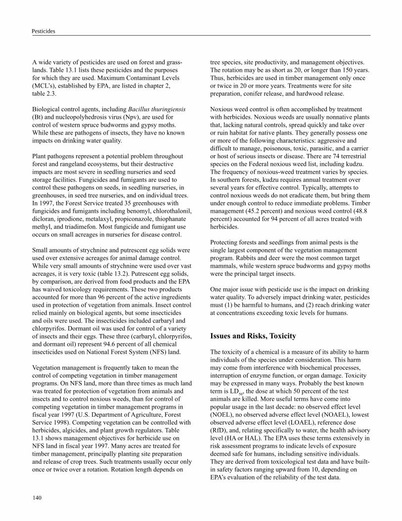
140
A wide variety of pesticides are used on forest and grass-
lands. Table 13.1 lists these pesticides and the purposes
for which they are used. Maximum Contaminant Levels
(MCL’s), established by EPA, are listed in chapter 2,
table 2.3.
Biological control agents, including Bacillus thuringiensis
(Bt) and nucleopolyhedrosis virus (Npv), are used for
control of western spruce budworms and gypsy moths.
While these are pathogens of insects, they have no known
impacts on drinking water quality.
Plant pathogens represent a potential problem throughout
forest and rangeland ecosystems, but their destructive
impacts are most severe in seedling nurseries and seed
storage facilities. Fungicides and fumigants are used to
control these pathogens on seeds, in seedling nurseries, in
greenhouses, in seed tree nurseries, and on individual trees.
In 1997, the Forest Service treated 35 greenhouses with
fungicides and fumigants including benomyl, chlorothalonil,
dicloran, iprodione, metalaxyl, propiconazole, thiophanate
methyl, and triadimefon. Most fungicide and fumigant use
occurs on small acreages in nurseries for disease control.
Small amounts of strychnine and putrescent egg solids were
used over extensive acreages for animal damage control.
While very small amounts of strychnine were used over vast
acreages, it is very toxic (table 13.2). Putrescent egg solids,
by comparison, are derived from food products and the EPA
has waived toxicology requirements. These two products
accounted for more than 96 percent of the active ingredients
used in protection of vegetation from animals. Insect control
relied mainly on biological agents, but some insecticides
and oils were used. The insecticides included carbaryl and
chlorpyrifos. Dormant oil was used for control of a variety
of insects and their eggs. These three (carbaryl, chlorpyrifos,
and dormant oil) represent 94.6 percent of all chemical
insecticides used on National Forest System (NFS) land.
Vegetation management is frequently taken to mean the
control of competing vegetation in timber management
programs. On NFS land, more than three times as much land
was treated for protection of vegetation from animals and
insects and to control noxious weeds, than for control of
competing vegetation in timber management programs in
fiscal year 1997 (U.S. Department of Agriculture, Forest
Service 1998). Competing vegetation can be controlled with
herbicides, algicides, and plant growth regulators. Table
13.1 shows management objectives for herbicide use on
NFS land in fiscal year 1997. Many acres are treated for
timber management, principally planting site preparation
and release of crop trees. Such treatments usually occur only
once or twice over a rotation. Rotation length depends on
tree species, site productivity, and management objectives.
The rotation may be as short as 20, or longer than 150 years.
Thus, herbicides are used in timber management only once
or twice in 20 or more years. Treatments were for site
preparation, conifer release, and hardwood release.
Noxious weed control is often accomplished by treatment
with herbicides. Noxious weeds are usually nonnative plants
that, lacking natural controls, spread quickly and take over
or ruin habitat for native plants. They generally possess one
or more of the following characteristics: aggressive and
difficult to manage, poisonous, toxic, parasitic, and a carrier
or host of serious insects or disease. There are 74 terrestrial
species on the Federal noxious weed list, including kudzu.
The frequency of noxious-weed treatment varies by species.
In southern forests, kudzu requires annual treatment over
several years for effective control. Typically, attempts to
control noxious weeds do not eradicate them, but bring them
under enough control to reduce immediate problems. Timber
management (45.2 percent) and noxious weed control (48.8
percent) accounted for 94 percent of all acres treated with
herbicides.
Protecting forests and seedlings from animal pests is the
single largest component of the vegetation management
program. Rabbits and deer were the most common target
mammals, while western spruce budworms and gypsy moths
were the principal target insects.
One major issue with pesticide use is the impact on drinking
water quality. To adversely impact drinking water, pesticides
must (1) be harmful to humans, and (2) reach drinking water
at concentrations exceeding toxic levels for humans.
Issues and Risks, Toxicity
The toxicity of a chemical is a measure of its ability to harm
individuals of the species under consideration. This harm
may come from interference with biochemical processes,
interruption of enzyme function, or organ damage. Toxicity
may be expressed in many ways. Probably the best known
term is LD50
, the dose at which 50 percent of the test
animals are killed. More useful terms have come into
popular usage in the last decade: no observed effect level
(NOEL), no observed adverse effect level (NOAEL), lowest
observed adverse effect level (LOAEL), reference dose
(RfD), and, relating specifically to water, the health advisory
level (HA or HAL). The EPA uses these terms extensively in
risk assessment programs to indicate levels of exposure
deemed safe for humans, including sensitive individuals.
They are derived from toxicological test data and have built-
in safety factors ranging upward from 10, depending on
EPA’s evaluation of the reliability of the test data.
Pesticides
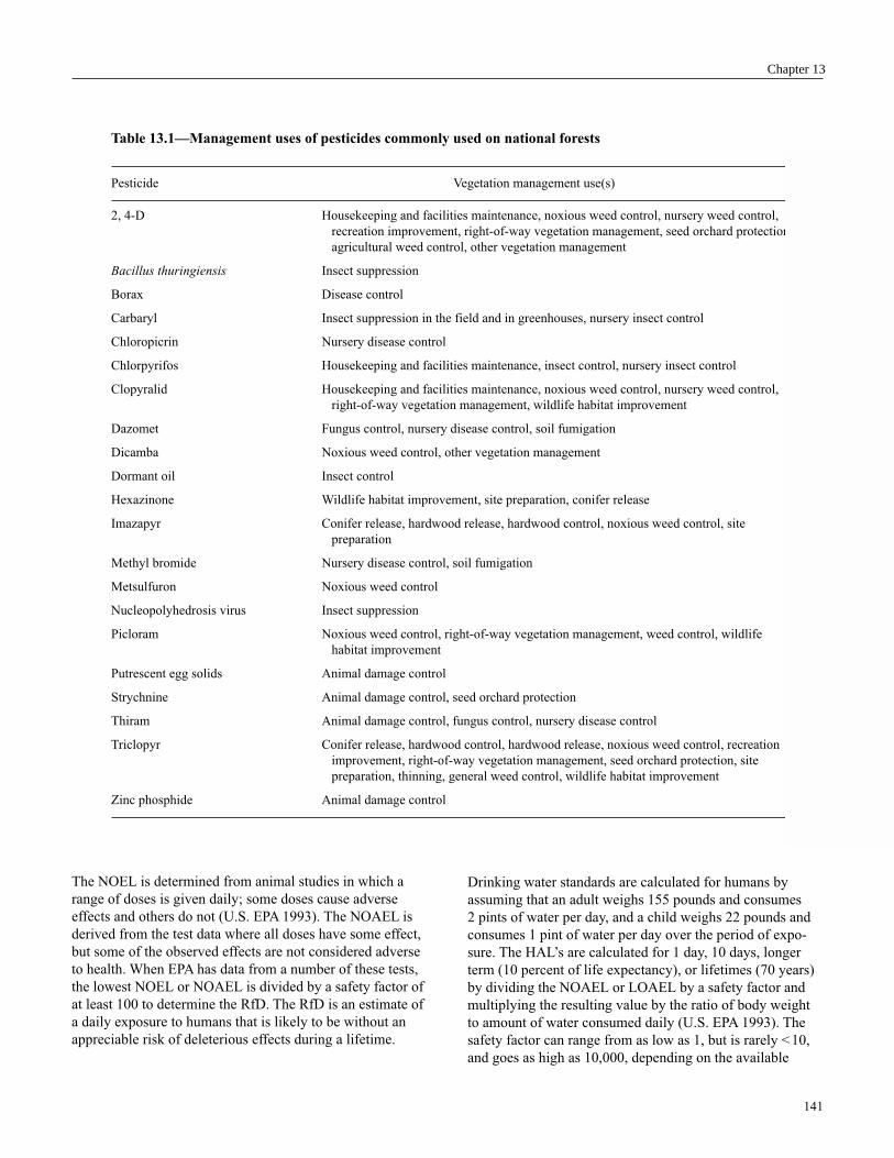
141
The NOEL is determined from animal studies in which a
range of doses is given daily; some doses cause adverse
effects and others do not (U.S. EPA 1993). The NOAEL is
derived from the test data where all doses have some effect,
but some of the observed effects are not considered adverse
to health. When EPA has data from a number of these tests,
the lowest NOEL or NOAEL is divided by a safety factor of
at least 100 to determine the RfD. The RfD is an estimate of
a daily exposure to humans that is likely to be without an
appreciable risk of deleterious effects during a lifetime.
Drinking water standards are calculated for humans by
assuming that an adult weighs 155 pounds and consumes
2 pints of water per day, and a child weighs 22 pounds and
consumes 1 pint of water per day over the period of expo-
sure. The HAL’s are calculated for 1 day, 10 days, longer
term (10 percent of life expectancy), or lifetimes (70 years)
by dividing the NOAEL or LOAEL by a safety factor and
multiplying the resulting value by the ratio of body weight
to amount of water consumed daily (U.S. EPA 1993). The
safety factor can range from as low as 1, but is rarely < 10,
and goes as high as 10,000, depending on the available
Table 13.1—Management uses of pesticides commonly used on national forests
Pesticide Vegetation management use(s)
2, 4-D Housekeeping and facilities maintenance, noxious weed control, nursery weed control,
recreation improvement, right-of-way vegetation management, seed orchard protection,
agricultural weed control, other vegetation management
Bacillus thuringiensis Insect suppression
Borax Disease control
Carbaryl Insect suppression in the field and in greenhouses, nursery insect control
Chloropicrin Nursery disease control
Chlorpyrifos Housekeeping and facilities maintenance, insect control, nursery insect control
Clopyralid Housekeeping and facilities maintenance, noxious weed control, nursery weed control,
right-of-way vegetation management, wildlife habitat improvement
Dazomet Fungus control, nursery disease control, soil fumigation
Dicamba Noxious weed control, other vegetation management
Dormant oil Insect control
Hexazinone Wildlife habitat improvement, site preparation, conifer release
Imazapyr Conifer release, hardwood release, hardwood control, noxious weed control, site
preparation
Methyl bromide Nursery disease control, soil fumigation
Metsulfuron Noxious weed control
Nucleopolyhedrosis virus Insect suppression
Picloram Noxious weed control, right-of-way vegetation management, weed control, wildlife
habitat improvement
Putrescent egg solids Animal damage control
Strychnine Animal damage control, seed orchard protection
Thiram Animal damage control, fungus control, nursery disease control
Triclopyr Conifer release, hardwood control, hardwood release, noxious weed control, recreation
improvement, right-of-way vegetation management, seed orchard protection, site
preparation, thinning, general weed control, wildlife habitat improvement
Zinc phosphide Animal damage control
Chapter 13
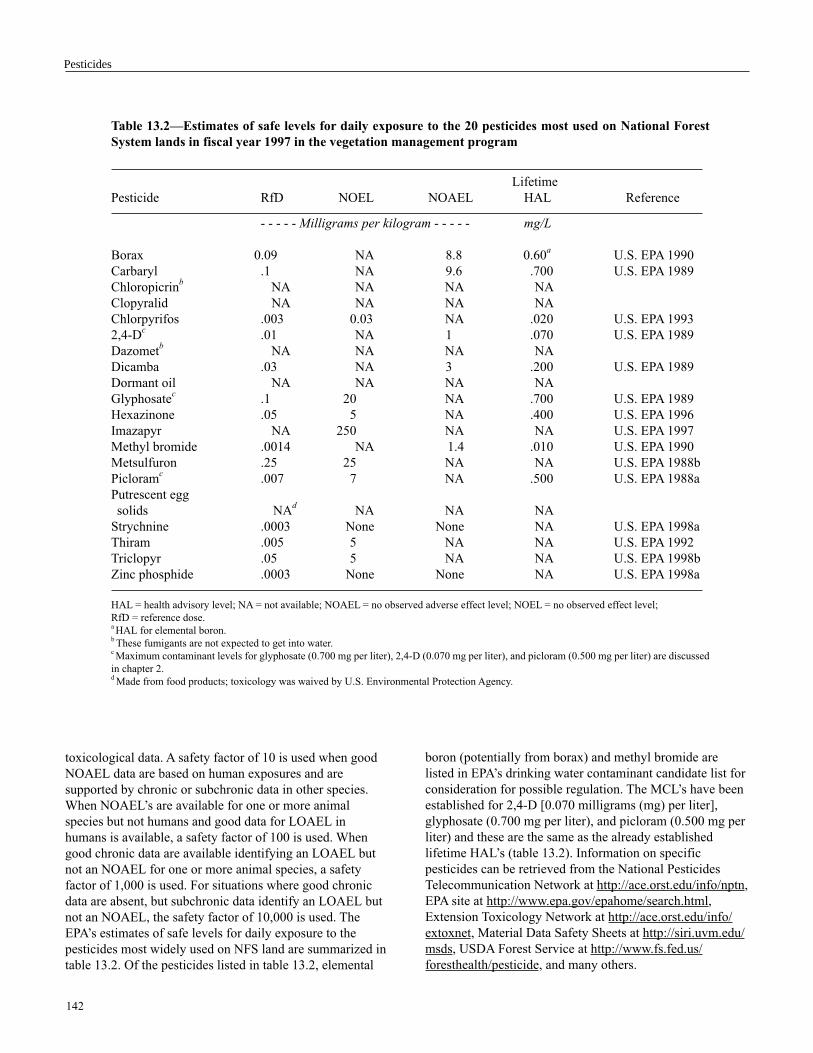
142
toxicological data. A safety factor of 10 is used when good
NOAEL data are based on human exposures and are
supported by chronic or subchronic data in other species.
When NOAEL’s are available for one or more animal
species but not humans and good data for LOAEL in
humans is available, a safety factor of 100 is used. When
good chronic data are available identifying an LOAEL but
not an NOAEL for one or more animal species, a safety
factor of 1,000 is used. For situations where good chronic
data are absent, but subchronic data identify an LOAEL but
not an NOAEL, the safety factor of 10,000 is used. The
EPA’s estimates of safe levels for daily exposure to the
pesticides most widely used on NFS land are summarized in
table 13.2. Of the pesticides listed in table 13.2, elemental
boron (potentially from borax) and methyl bromide are
listed in EPA’s drinking water contaminant candidate list for
consideration for possible regulation. The MCL’s have been
established for 2,4-D [0.070 milligrams (mg) per liter],
glyphosate (0.700 mg per liter), and picloram (0.500 mg per
liter) and these are the same as the already established
lifetime HAL’s (table 13.2). Information on specific
pesticides can be retrieved from the National Pesticides
Telecommunication Network at http://ace.orst.edu/info/nptn,
EPA site at http://www.epa.gov/epahome/search.html,
Extension Toxicology Network at http://ace.orst.edu/info/
extoxnet, Material Data Safety Sheets at http://siri.uvm.edu/
msds, USDA Forest Service at http://www.fs.fed.us/
foresthealth/pesticide, and many others.
Table 13.2—Estimates of safe levels for daily exposure to the 20 pesticides most used on National Forest
System lands in fiscal year 1997 in the vegetation management program
Lifetime
Pesticide RfD NOEL NOAEL HAL Reference
- - - - - Milligrams per kilogram - - - - - mg/L
Borax 0.09 NA 8.8 0.60a
U.S. EPA 1990
Carbaryl .1 NA 9.6 .700 U.S. EPA 1989
Chloropicrinb
NA NA NA NA
Clopyralid NA NA NA NA
Chlorpyrifos .003 0.03 NA .020 U.S. EPA 1993
2,4-Dc
.01 NA 1 .070 U.S. EPA 1989
Dazometb
NA NA NA NA
Dicamba .03 NA 3 .200 U.S. EPA 1989
Dormant oil NA NA NA NA
Glyphosatec
.1 20 NA .700 U.S. EPA 1989
Hexazinone .05 5 NA .400 U.S. EPA 1996
Imazapyr NA 250 NA NA U.S. EPA 1997
Methyl bromide .0014 NA 1.4 .010 U.S. EPA 1990
Metsulfuron .25 25 NA NA U.S. EPA 1988b
Picloramc
.007 7 NA .500 U.S. EPA 1988a
Putrescent egg
solids NAd
NA NA NA
Strychnine .0003 None None NA U.S. EPA 1998a
Thiram .005 5 NA NA U.S. EPA 1992
Triclopyr .05 5 NA NA U.S. EPA 1998b
Zinc phosphide .0003 None None NA U.S. EPA 1998a
HAL = health advisory level; NA = not available; NOAEL = no observed adverse effect level; NOEL = no observed effect level;
RfD = reference dose.a HAL for elemental boron.
b These fumigants are not expected to get into water.
c Maximum contaminant levels for glyphosate (0.700 mg per liter), 2,4-D (0.070 mg per liter), and picloram (0.500 mg per liter) are discussed
in chapter 2.d Made from food products; toxicology was waived by U.S. Environmental Protection Agency.
Pesticides
143
Findings from Studies
Pesticides used by the NFS in vegetation management are
used around the World in agricultural, forest, range, and
urban applications. Some have been found in surface water,
shallow ground water, and even in shallow wells (< 30 ft),
but in concentrations far below levels harmful to human
health, and the occurrence is infrequent. Table 13.3 summa-
rizes reports of pesticides from table 13.2 that have been
detected in water in the United States.
Larson and others (1997) summarized the results of 236
studies throughout the United States on pesticide contamina-
tion of surface water by listing the maximum observed
concentrations from each study. These studies were located
principally around large river drainage basins and, therefore,
represent cumulative pesticide contributions from a wide
variety of uses. Monitoring results were reported for 52
pesticides approved for agricultural, urban, and forestry use
and their metabolic byproducts. Of the pesticides listed in
table 13.2, only six were reported to be present in surface
water by Larson and others (1997). They were carbaryl,
1 report; hexazinone, 1 report; chlorpyrifos, 3 reports;
picloram, 4 reports; dicamba, 5 reports; and 2,4-D, 24
reports. None of the reported concentrations exceeded EPA
safe levels for human health except where application
included placement directly in stream channels and most
were < 0.002 mg per liter. It is important to recognize that
surface water is not necessarily drinking water. The studies
summarized by Larson and others (1997) dealt with surface
water, principally in lakes, reservoirs, and rivers, which
would be treated prior to use for drinking. Thus, use of these
pesticides according to label directions has not resulted in
impairment of drinking water.
Reports of pesticide contamination of water are usually from
agricultural (Kolpin and others 1997, Koterba and others
1993) or urban applications (Bruce and McMahon 1996),
but the potential exists for contamination from forest
vegetation management. Water from forests is generally
much less contaminated than water from other land uses.
Several studies on forest sites listed in table 13.3 present
data for water collected directly from treated areas. The
concentration of pesticides can appear quite high compared
to samples taken from large rivers and lakes. Pesticide
concentrations are greatly reduced by dilution as they move
from the treated sites to downstream locations. Degradation
of pesticides by biological, hydrolytic, and photolytic routes
also contributes to downstream reductions in pesticide
concentrations.
From 1985–87, Cavalier and others (1989) monitored 119
wells, springs, and municipal water supplies for occurrence
of pesticides in drinking water throughout the State of
Arkansas. Monitored wells were generally located in the
eastern portion of Arkansas, but eight wells were located in
the Ouachita National Forest. Only sites considered highly
susceptible to contamination from pesticide use were
monitored, and these included domestic, municipal, and
irrigation wells. Detection limits for the three forestry
pesticides monitored (2,4-D, hexazinone, and picloram)
ranged from 70 to 800 times lower than their HAL’s. They
did not detect well water contamination from any of the 18
pesticides for which they monitored. Failure to detect
pesticides in these wells believed to be at high risk for
contamination is a very strong indicator that ground water is
not at risk from forestry pesticides used according to label
directions.
Michael and Neary (1993) reported on 23 studies conducted
on industrial forests in the South in which whole watersheds
received herbicide treatment. Water flowing from the sites
was sampled near the downstream edge of the treatments.
The watersheds were relatively small (< 300 acres) and the
ephemeral to first-order streams draining these watersheds
were too small to be public drinking water sources, but their
flow reached downstream reservoirs. The maximum
observed hexazinone, imazapyr, picloram, and sulfometuron
concentrations in streams on these treated sites did not
exceed HAL’s, except for one case in which hexazinone was
experimentally applied directly to the stream channel. Even
in this case in which hexazinone was applied directly to the
stream at a very high rate, drinking water standards were
exceeded for only a few hours. In another study, picloram
was accidentally applied directly to streams, but maximum
picloram concentrations did not exceed HAL’s during the
year after application.
Bush and others (1990) reported on use of hexazinone on
two Coastal Plain sites (deep sand and sandy loam soils) that
were monitored for impacts on ground water. Hexazinone
was not detected in ground water at the South Carolina site
for 2 years after application. In Florida, hexazinone was
found infrequently in shallow test wells at concentrations up
to 0.035 mg per liter, much lower than the safe levels for
daily exposure (0.400 mg per liter). Water from these sites
drains into other creeks and rivers and is diluted before
entering reservoirs.
Michael and others (1999) reported the dilution of
hexazinone downstream of treated sites. One mile below
the treated site, hexazinone concentrations were diluted to
one-third to one-fifth the concentration observed on the
treated site. Hexazinone was applied for site preparation at
6 pounds active ingredient (ai) per acre to clay loam soils,
a rate three times the normal, and it was applied directly to
Chapter 13

144
Table 13.3—Frequency and occurrence of surface and ground water contamination from pesticide use in North
Americaa
Water
Pesticide type Location Maximum Range Comments Reference
- - - - - Milligrams per liter - - - - -
2, 4-D S Large river basins 0.0075 0.00004 – 0.0075 Twenty-four reports of mainly Larson and others 1997
throughout the urban, suburban, agricultural
United States sources
S Streams in Oregon 2.0 ND – 2.0 Highest concentrations observed Norris 1981
and California from forest areas where no
attempt was made to prevent
application to water
G Saskatchewan,
Canada .0000007 NG Natural spring flow Wood and Anthony 1997
G Connecticut, Iowa, .049 .0002 – .049 Well water samples, except for Funari and others 1995
Kansas, Maine, South Dakota, from shallow
Mississippi, South sand and gravel aquifer
Dakota
Borax NR NR NR NR NR
Carbaryl S Mississippi River .0001 NG One report Larson and others 1997
S New Brunswick, .314 NG Aerial spray spruce budworm Sundaram and Szeto 1987
Canada control
S New Brunswick,
Canada .314 .123 – .314 Budworm control Holmes and others 1981
Chloropicrin NR NR NR NR NR
Chlorpyrifos S Mississippi River, .00015 .00004 – .00015 Three reports Larson and others 1997
the lower Colorado
River, rivers and lakes
in Kansas, irrigation
ditches in California
Arizona, Nevada
Clopyralid NR NR NR NR NR
Dazomet NR NR NR NR NR
Dicamba S USFS land near .037 .006 – .037 Treated 166 ac of 603-ac forest Norris 1975
Hebo, OR catchment; highest concentration
diluted to 0.006 mg/L 2.2 mi
downstream
Glyphosate S 45-ha coastal British .162 .0032 – .162 Highest concentration in streams Feng and others 1990
Columbian catchment intentionally sprayed, lowest
in streams with smz
S Quebec, Canada 3.080 .078 – 3.08 Nine of 36 streams contained Leveille and others 1993
glyphosate after forest spraying
S Ohio 5.2 NG No-tillage establishment of fescue Edwards and others 1980
S Georgia .035 NG Forest sites for scrub-hardwood Newton and others 1994
Michigan 1.237 NG control and direct spray of
Oregon .031 NG streams
continued
Pesticides

145
Table 13.3—Frequency and occurrence of surface and ground water contamination from pesticide use in North
Americaa (continued)
Water
Pesticide type Location Maximum Range Comments Reference
- - - - - Milligrams per liter - - - - -
Glyphosate
(cont.) G Newfoundland, 0.045 0.004 – 0.045 Application of 4 lbs ai/ac to power Smith and others 1996
Canada substations resulted in contamina-
tion of water in monitoring wells
Hexazinone S Mississippi River .00007 NG Detected in five tributaries Larson and others 1997
S Alabama, Florida, .037 .0013 – 0.037 Seven reports, each treated Michael and Neary 1993
Georgia catchment containing ephemeral/
first-order streams
S Alabama 2.400 NG Applied directly to ephemeral Miller and Bace 1980
channel and in first runoff water
S Alabama .473 .422 – .473 Ephemeral/first-order stream in Michael and others 1999
catchments treated with 3x rate of
hexazinone in liquid and pellet
formulation with accidental
application to streams
S Arkansas .014 NG 11.5-ha watershed drained by Bouchard and others 1985
ephemeral to first-order stream
S Georgia .442 NG Ephemeral/first-order stream Neary and others 1986
in treated catchment, pellets
applied to stream channel
G NGb .009 NG Only one value reported from a Funari and others 1995
single study
Imazapyr S Alabama .680 .130 – .680 Two reports, each treated catch- Michael and Neary 1993
ment containing ephemeral/
first-order streams, herbicide
accidentally applied to stream
channel
Methyl
bromide NR NR NR NR NR
Metsulfuron S Central Florida .008 NG Water in surface depression Michael and others 1991
G .002 NG in slash pine site and 1 of 207
shallow (6-ft) well samples
Picloram S North-central
Arizona .32 NG Pinyon-juniper site Johnsen 1980
S Streams and rivers .005 .00001 – .005 Four reports from mainly range- Larson and others 1997
in North Dakota, land uses
Wyoming, Montana
S Alabama .442 NG Pellets accidentally applied Michael and others 1989
directly to forest stream
S Georgia, Kentucky, .021 ND – .021 Six study catchments with Michael and Neary 1993
Tennessee ephemeral/first-order stream in
each treated forest catchment
S North Carolina .01 NG Ephemeral/first-order stream in Neary and others 1985
treated forest catchment
continued
Chapter 13

146
a stream segment, resulting in a maximum observed on-site
concentration of 0.473 mg per liter. This was slightly more
than the lifetime HAL but considerably below the longer
term HAL of 9.0 mg per liter (U.S. EPA 1990). Following
the application, on-site stream concentrations did not exceed
the lifetime HAL.
Norris (1975) reported contamination of streamflow with
dicamba used for control of hardwoods on silty clay loam
soils in Oregon. On a 603-acre watershed, 166 acres were
aerially sprayed with 1 pound ai per acre [1.1 kilograms (kg)
per hectare] of dicamba. A small stream segment was also
sprayed causing detectable dicamba residues 2 hours after
application began, approximately 0.8 miles (1.3 kilometers)
downstream. Concentrations rose for approximately 5.2
hours after treatment began and reached a maximum
concentration of 0.037 mg per liter, less than one-fifth of
the HAL (0.200 mg per liter). No dicamba residues were
detected beyond 11 days after treatment.
Glyphosate and 2,4-D have aquatic labels, which permit
direct application to water. Stanley and others (1974) found
that when 2,4-D was applied to reservoirs for aquatic weed
control, about half of water samples from within treatment
areas contained 2,4-D, and the highest concentration
(0.027 mg per liter) was less than half of the HAL (0.070
mg per liter). Newton and others (1994) aerially applied
glyphosate at three times the normal forestry usage rate [4
pounds ai per acre (4.4 kg per hectare)], no buffers were left,
and all streams and ponds were sprayed. Initial water
concentrations were 0.031 and 0.035 mg per liter in Oregon
and Georgia, respectively, and 1.237 mg per liter in Michi-
gan on the day of application. After day one, glyphosate
concentrations dropped to below 0.008 mg per liter on all
three sites for the duration of the study. The HAL was
exceeded on only one of three sites and then for only 1 day.
There is little information on the movement of metsulfuron
to streams. Michael and others (1991) found trace residues
of metsulfuron in shallow monitoring wells in Florida where
24 wells were sampled to a depth of 6 feet (1.8 meters).
Metsulfuron was detected (0.002 mg per liter) in 1 of 207
samples collected during 2 months after application.
Pesticides movement into streams is well documented, but
movement into ground water is not well researched. During
movement from streamwater into ground water, concentra-
tions should be reduced considerably for several reasons.
Infiltrating pesticides must pass through several physical
barriers or layers before reaching ground water. As they pass
Table 13.3—Frequency and occurrence of surface and ground water contamination from pesticide use in North Americaa
(continued)
Water
Pesticide type Location Maximum Range Comments Reference
- - - - - Milligrams per liter - - - - -
Picloram
(cont.) G Saskatchewan,
Canada 0.000225 NR Natural spring flow Wood and Anthony 1997
G Iowa, Maine, .049 0.00063 – 0.049 Fewer than 2% of well samples Funari and others 1995
Minnesota, were positive
North Dakota
Strychnine NR NR NR NR NR
Thiram NR NR NR NR NR
Triclopyr S Florida .002 NG Coastal Plain flatwoods catch- Bush and others 1988
ments near Gainesville, FL
S Ontario, Canada .35 .23 – .35 Intentional aerial application Thompson and others 1991
to boreal forest stream
Zinc
phosphide NR NR NR NR NR
Ai = active ingredient; G = ground water; ND = not detected; NG = not given; NR = no reports found in published literature; S = surface water;
smz = streamside management zone; USFS = USDA Forest Service.a This table summarizes the levels of pesticides reported in the literature at specific sites and is representative of the literature from North America. However, it
cannot be extrapolated for purposes of prediction.b The authors do not provide specific location.
Pesticides

147
through each layer, they are degraded, diluted, and metabo-
lized. Surface water provides a medium for dilution,
hydrolysis, and photolysis. Aquatic vegetation can metabo-
lize pesticides. Microbes associated with coarse and fine
particulate organic matter found naturally in streams also
metabolize pesticides.
In order for water on the soil surface to carry pesticides into
ground water, it must pass through the soil column. Here
again, processes work to reduce the potential for pesticides
to reach ground water. Pesticides percolating through the
soil column are adsorbed to soil particles, reducing the
amount reaching the ground water. Pesticides adsorbed onto
soil particles may be irreversibly bound, released slowly, or
further metabolized by microbes. Once pesticides reach
ground water, they may degrade further. Cavalier and others
(1991) found that microbes degraded herbicides, including
2,4-D, in ground water.
Thus, ground water concentrations of pesticides should be
considerably lower than observed in surface water. Funari
and others (1995) reviewed the literature and reported the
range of maximum ground water concentrations of pesti-
cides, including those used in forestry, agriculture, home
and garden, and on industrial rights-of-way. The maximum
range of values for 2,4-D (0.0002 to 0.0495 mg per liter),
hexazinone (0.009 mg per liter), and picloram (0.00063 to
0.049 mg per liter) are much lower than the HAL’s for those
compounds.
The National Water-Quality Assessment Program
(NAWQA) conducted by the U.S. Geological Survey began
in 1991. The focus of NAWQA is to identify nutrient and
pesticide contamination of water throughout the United
States. The 1999 NAWQA report (found at http://water.usgs.
gov/pubs/circ/circ1225/index.html) makes little mention of
forest sites or forestry pesticides, but concludes that:
“Concentrations of nutrients and pesticides in streams and
shallow groundwater generally increase with increasing
amounts of agricultural and urban land in a watershed.” The
report focused on more than 50 major river basins and
aquifers supplying water to more than 60 percent of the
population and approximately half of the area of the United
States. Few forestry pesticides other than 2,4-D were found
in these basins or aquifers.
Even in predominantly agriculture areas, the report states:
One of the most striking results for shallow ground-
water in agricultural areas, compared with streams, is
the low rate of detection for several high-use herbi-
cides other than atrazine. This is probably because
these herbicides break down faster in the natural
environment compared to atrazine.
Atrazine is principally used in growing corn (maze). It has
not been used on NFS land since 1992. While not directly
addressing forestry pesticides and drinking water, these
NAWQA conclusions support the above research findings
and conclusions that ground water contamination by
pesticides should be lower than observed for surface water.
Because surface water contamination from forest sites
treated according to label directions does not exceed HAL’s,
it is very unlikely that ground water contamination would
exceed HAL’s.
Several of the pesticides in table 13.2 have not been
reported in water. They include chloropicrin, chlopyralid,
dazomet, and thiram. Chloropicrin and dazomet are soil
fumigants, which are gases in their active form and are used
only for seedling production. Chlopyralid is a relatively new
compound in the United States. Thiram is a dimethyl
dithiocarbamate fungicide, principally used in forestry for
seed protection.
There is very little water-quality data for pesticides used in
nursery disease control and soil fumigation. More than 71
percent of fungicides and fumigants used on NFS land are
applied in nurseries. Intense use in a nursery may result in
localized ground water contamination. Three pesticides
(chloropicrin, dazomet, and methyl bromide) make up this
group of intensively used agents. Chloropicrin is toxic to
plants and is used in combination with other chemicals for
fumigating seedbeds. Dazomet, a soil fumigant, is a gas and
is relatively insoluble in water (3 grams per liter). However,
dazomet is unstable in water and quickly breaks down into
methyl isothiocyanate (MITC), formaldehyde, mono-
methylamine, and hydrogen sulfide. All are toxic, but the
most toxic is MITC. The RfD for formaldehyde is 0.2 mg
per kilogram per day. However, EPA has classified formal-
dehyde as a compound of medium carcinogenic hazard to
humans. Methyl bromide is very toxic. Data are insufficient
to determine whether frequent use of these three pesticides
adversely impacts water quality, either locally or over an
expanded area.
Reliability and Limitation of Findings
Most data reviewed in this chapter come from scientific
literature. The data listed in table 13.3 and derived from
Larson and others (1997) were extracted from in-house
reports from the U.S. Geological Survey, the EPA, State,
and local governmental departments for the environment
and scientific literature. Reports published in scientific
literature are the most reliable because they were subject
to peer review and scrutiny for validity of methods,
Chapter 13

148
completeness of data, and interpretation of the data.
Monitoring data from in-house publications and reports may
be less reliable.
Some variability in results of individual studies is due to
regional soil and climate differences. In the South, infiltra-
tion rates on many forestry sites are generally low, owing to
the highly eroded condition of the soils. Here, precipitation
intensity frequently exceeds infiltration rates, producing
overland flow on newly prepared sites. Overland flow may
lead to much higher pesticide concentrations in stormflow
than in other areas of the country with much higher infiltra-
tion rates. Very high infiltration rates are typical of soils in
the Pacific Northwest. Therefore, if streams are protected by
buffers, broadcast application of pesticides generally results
in stream contamination either via direct application or
through baseflow contributions. In general, levels of
contamination are lowest where infiltration rates are highest.
Care must always be exercised in extrapolating data from
local studies on drinking water to a regional or larger scale.
However, three strategies of worst-case scenarios used in
these studies mitigate against high levels of uncertainty:
(1) several studies have investigated the impacts of pesti-
cides applied directly to surface water; (2) several studies
have investigated the impacts on water of pesticides applied
at several times the prescribed rate; and (3) most of the
studies conducted specifically on forestry sites treated the
entire catchment from which water samples were taken,
resulting in samples with levels of pesticide contamination
greater than are likely to occur anywhere downstream.
Research on the impacts of pesticides applied directly to
surface water used the worst-case scenario for forest
operational treatments in which pesticide was applied at
normal rates directly to surface water (ponds and streams).
These studies did not find any contamination of water at
levels above the HAL for any pesticide studied. Research on
aquatic impacts from pesticides applied at several times the
labeled rate used the worst-case scenario for operational
treatments where an area might receive multiple
applications in error or where small spills occurred. In these
studies, HAL’s were exceeded by only a few percent and
only briefly, usually for less than a few hours. Both worst-
case scenarios just described were combined with the third
worst-case scenario in which all sampling was conducted on
surface water found within the treated area. In this case,
most of the water was in small pools or ephemeral to first-
order streams. While ephemeral to first-order streams or
pools are unlikely to be drinking water sources because of
low yield, they do represent water most likely to be severely
contaminated from normal forest pesticide applications.
Even these waters were not contaminated at levels
exceeding HAL’s, except where pesticide was applied at
several times the labeled rate as described above.
In addition, data on contamination of water for the pesti-
cides in table 13.3 have been taken from a number of studies
conducted in North America and the findings are generally
similar. These studies have, with a few exceptions, con-
firmed the absence of significant contamination of drinking
water. The exceptions were those cases in which a pesticide
was applied directly to water, and the high concentrations
observed in those studies were at or only slightly above
drinking water standards. These high concentrations lasted
only a few hours at most before dropping well below current
HAL’s. It is clear from the available literature that use of
pesticides in strict accordance with label directions on NFS
land cannot be expected to contribute significantly to ground
water or drinking water contamination. It is also clear that
pesticides, unless clearly labeled for aquatic uses, must not
be applied directly to water, and that pesticides should be
used around water resources, which are particularly sensi-
tive only after careful consideration of the ramifications.
Limitations of the data are obvious for the few chemicals
that have not been investigated. We need data on them as
well as other chemicals about which little information is
available. Additional limitations include lack of sufficient
testing for health effects as indicated in table 13.2. The
question of cumulative toxicological effects has not been
addressed for any of the pesticide mixtures utilized in
modern forest management.
Research Needs
Several issues related to vegetation management need
additional research.
1. One issue is impacts of frequent, repeated use of fungi-
cides and fumigants in nursery operations on nearby
water quality.
2. Another issue is effectiveness of buffer width and
composition. There is too little information on the
processes and interactions of site-specific characteristics
with pesticide chemistry that permit buffers to mediate
against contamination of streams and surface waters in
general. These processes and the interactions of pesticide
chemistry with site-specific conditions must be identified
and understood so managers can design and install
optimally functional buffers to protect the water resource
and its associated aquatic ecosystem.
Pesticides

149
3. A third issue is that several pesticides in table 13.3 lack
published reports relating their use to occurrence in
water.
4. Still another issue is the effects of commonly used
pesticide mixtures, as opposed to single compounds, on
the water resource.
Key Points
Relative to agricultural, urban, and other uses of pesticides,
very small amounts are used on NFS land. Further, the use
patterns for any specific piece of land are infrequent, except
in the case of vegetation protection from pathogens,
animals, and insects where annual treatment may be
required, especially in greenhouses and nurseries. Pesticides
used on NFS land are also used around the World to
accomplish management goals similar to those on NFS land,
but often in a much more intensive way. Even with the
widespread use of pesticides in North America, those
typically used on NFS land have not been identified in
surface or ground water at sufficiently high concentrations
as to cause drinking water problems. Their rapid break down
by physical, chemical, and biological routes coupled with
use patterns precludes the development of water contamina-
tion problems unless they are applied directly to water. Even
though these same pesticides are used around homes, in
urban and in agricultural settings, their use in forest manage-
ment is still controversial in the public arena. Therefore,
their use should be carefully planned and all agency, local,
State, and Federal laws should be followed. It is especially
important to follow all label directions because pesticide
labels are legal documents specifying Federal laws pertain-
ing to their use. Best management practices should be
carefully adhered to and use around drinking water supplies
should be avoided, except where permitted by the label.
Wherever pesticides are used, precautions should always be
taken to protect drinking water sources from contamination.
Literature Cited
Bouchard, D.C.; Lavy, T.L.; Lawson, E.R. 1985. Mobility and persis-
tence of hexazinone in a forest watershed. Journal of Environmental
Quality. 14: 229–233.
Bruce, B.W.; McMahon, P.B. 1996. Shallow ground-water quality beneath
a major urban center. Journal of Hydrology. 186: 129–151.
Bush, P.B.; Michael, J.L.; Neary, D.G.; Miller, K.V. 1990. Effect of
hexazinone on groundwater quality in the Coastal Plain. Proceedings of
the Southern Weed Science Society; 1990 January 15–17; Atlanta.
Champaign, IL: Southern Weed Science Society. 43: 184–194.
Bush, P.B.; Neary, D.G.; Taylor, J.W. 1988. Effect of triclopyr amine and
ester formulations on groundwater and surface runoff water quality in
the Coastal Plain. Proceedings of the Southern Weed Science Society;
1988 January 18–20; Tulsa, OK. Champaign, IL: Southern Weed Science
Society. 41: 226–232.
Cavalier, T.C.; Lavy, T.L.; Mattice, J.D. 1989. Assessing Arkansas
ground water for pesticides: methodology and findings. Ground Water
Monitoring Review. 9: 159–166.
Cavalier, T.C.; Lavy, T.L.; Mattice, J.D. 1991. Persistence of selected
pesticides in ground-water samples. Ground Water. 29: 225–231.
Comerford, N.B.; Neary, D.G.; Mansell, R.S. 1992. The effectiveness of
buffer strips for ameliorating offsite transport of sediment, nutrients, and
pesticides from silvicultural operations. Tech. Bull. 631. Research
Triangle Park, NC: National Council of the Paper Industry for Air and
Stream Improvement. 48 p.
Edwards, W.M.; Triplett, G.B., Jr.; Kramer, R.M. 1980. A watershed
study of glyphosate transport in runoff. Journal of Environmental
Quality. 9(4): 661–665.
Feng, J.C.; Thompson, D.G.; Reynolds, P.E. 1990. Fate of glyphosate in
a Canadian forest watershed. 1: Aquatic residues and off-target deposit
assessment. Journal of Agricultural and Food Chemistry. 38(4):
1110–1118.
Funari, E.; Donati, L.; Sandroni, D.; Vighi, M. 1995. Pesticide levels in
groundwater: value and limitations of monitoring. In: Vighi, M.; Funari,
E., eds. Pesticide risk in groundwater. Boca Raton, FL: Lewis Publish-
ers. 275 p.
Holmes, S.B.; Millikin, R.L.; Kingsbury, P.D. 1981. Environmental effects
of a split application of Sevin–2–oil. Rep. FPM–X–46. Sault Ste. Marie,
Ontario: Canadian Forestry Service. 58 p.
Johnsen, T.N., Jr. 1980. Picloram in water and soil from a semiarid
pinyon-juniper watershed. Journal of Environmental Quality. 9:
601–605.
Kolpin, D.W.; Kalkhoff, S.J.; Goolsby, D.A. [and others]. 1997.
Occurrence of selected herbicides and herbicide degradation products in
Iowa’s ground water, 1995. Ground Water. 35: 679–688.
Koterba, M.T.; Banks, W.S.L.; Shedlock, R.J. 1993. Pesticides in
shallow groundwater in the Delmarva Peninsula. Journal of Environ-
mental Quality. 22: 500–518.
Larson, S.J.; Capel, P.D.; Majewski, M.S. 1997. Pesticides in surface
water: distribution, trends, and governing factors. Ser. 5.3: Pesticides in
the hydrologic system. Chelsea, MI: Ann Arbor Press. 373 p.
Leveille, P.; Legris, J.; Couture, G. 1993. Results of spot checks in lotic
environments after spraying of glyphosate in forests from 1989 to 1991.
Quebec, Canada: Ministere des Forets du Quebec. 21 p.
Michael, J.L.; Neary, D.G. 1993. Herbicide dissipation studies in southern
forest ecosystems. Environmental Toxicology and Chemistry. 12:
405–410.
Michael, J.L.; Neary, D.G.; Fischer, J.B.; Gibbs, H.G. 1991.
Metsulfuron in surface groundwater of a north Florida flatwoods.
Proceedings of the Southern Weed Science Society; 1991 January
14–16; San Antonio, TX. Champaign, IL: Southern Weed Science
Society. 44: 233–237.
Chapter 13

150
Michael, J.L.; Neary, D.G.; Wells, M. 1989. Picloram movement in soil
solution and streamflow from a Coastal Plain forest. Journal of
Environmental Quality. 18: 89–95.
Michael, J.L.; Webber, E.C.; Bayne, D.R. [and others]. 1999.
Hexazinone dissipation in forest ecosystems and impacts on aquatic
communities. Canadian Journal of Forest Research. 29: 1170–1181.
Miller, J.H.; Bace, A.C. 1980. Streamwater contamination after aerial
contamination of a pelletized herbicide. Res. Note SO–255. New
Orleans: U.S. Department of Agriculture, Forest Service, Southern
Forest Experiment Station. 4 p.
Neary, D.G.; Bush, P.B.; Douglas, J.E.; Todd, R.L. 1985. Picloram
movement in an Appalachian hardwood forest watershed. Journal of
Environmental Quality. 14: 585–592.
Neary, D.G.; Bush, P.B.; Grant, M.A. 1986. Water quality of ephemeral
streams after site preparation with the herbicide hexazinone. Forest
Ecology and Management. 14: 23–40.
Newton, M.; Horner, L.M.; Cowell, J.E. [and others]. 1994. Dissipation
of glyphosate and aminomethylphosphonic acid in North American
forests. Journal of Agricultural and Food Chemistry. 42: 1795–1802.
Norris, L.A. 1975. Dicamba residues in streams after forest spraying.
Bulletin of Environmental Contamination and Toxicology. 13: 1–8.
Norris, L.A. 1981. Phenoxy herbicides and TCDD in forests. Residue
Reviews. 80: 65–135.
Pimentel, D.; Levitan, L. 1986. Pesticides: amounts applied and amounts
reaching pests. BioScience. 36(2): 86–91.
Smith, N.J.; Martin, R.C.; St. Croix, R.G. 1996. Levels of the herbicide
glyphosate in well water. Bulletin of Environmental Contamination and
Toxicology. 57: 759–765.
Stanley, R.A.; Bates, A.L.; Bedsole, J.A.; Hall, T.F. 1974. Program
diversity and control of Eurasian watermilfoil in Tennessee Valley
reservoirs. In: Proceedings of the Weed Science Society of America;
1974 February 12–16; Las Vegas, NV: Champaign, IL: Southern Weed
Science Society. 19 p.
Sundaram, K.M.S.; Szeto, S.Y. 1987. Distribution and persistance of
carbaryl in some terrestrial and aquatic components of a forest
environment. Journal of Environmental Science and Health, B
(Pesticides, Food Contaminants and Agricultural Wastes). B22:
5, 579–599.
Thompson, D.G.; Staznik, B.; Fontaine, D.D. [and others]. 1991. Fate
of triclopyr ester released in a boreal forest stream. Environmental
Toxicology and Chemistry. 10(5): 619–632.
U.S. Department of Agriculture, Forest Service. 1998. Report of the Forest
Service fiscal year 1997. Washington, DC: U.S. Department of Agricul-
ture, Forest Service. 147 p.
U.S. EPA. 1988a. Picloram health advisory. Washington, DC: U.S.
Environmental Protection Agency, Office of Drinking Water. 18 p.
U.S. EPA. 1988b. U.S. EPA integrated risk information system substance
file–Ally. CASRN 74223–64–6. Washington, DC: U.S. Environmental
Protection Agency. [Not paged]. [Available on the Web at: http://
www.epa.gov/ngispgm3/iris/subst/0288.htm].
U.S. EPA. 1989. Drinking water health advisory. Pesticides. U.S.
Environmental Protection Agency, Office of Drinking Water Health
Advisories. Chelsea, MI: Lewis Publishers, Inc. 819 p.
U.S. EPA. 1990. Drinking water regulations and health advisories.
Washington, DC: U.S. Environmental Protection Agency, Office of
Drinking Water. 10 p.
U.S. EPA. 1992. U.S. EPA integrated risk information system substance
file — Thiram. CASRN 137–26–8. Washington, DC: U.S. Environmen-
tal Protection Agency. [Not paged]. [Available on the Web at: http://
www.epa.gov/ngispgm3/iris/subst/0267.htm].
U.S. EPA. 1993. Health advisories for drinking water contaminants. U.S.
Environmental Protection Agency, Office of Water Health Advisories.
Boca Raton, FL: Lewis Publishers. 261 p.
U.S. EPA. 1996. Hexazinone health advisory. Washington, DC: U.S.
Environmental Protection Agency, Office of Drinking Water. 24 p.
U.S. EPA. 1997. Imazapyr (Arsenal) pesticide tolerances: final rule.
Pesticide management education program. Ithaca, NY: Cornell
University. [Not paged]. [Available on the Web at: http://
pmep.cce.cornell.edu/profiles/herb-growthreg/fatty-alcohol-monuron/
imazapyr/tol-imazapyr.html#top].
U.S. EPA. 1998a. Draft Resource Conservation and Recovery Act; waste
minimization PBT chemical list; app. C: Waste minimization
prioritization tool human noncancer scores. Washington, DC: U.S.
Environmental Protection Agency, Office of Solid Waste, Waste
Minimization Branch. [Not paged]. [Available on the Web at: http://
www.epa.gov/epaoswer/hazwaste/minimize/chemlist/ap_c.pdf].
U.S. EPA. 1998b. Reregistration eligibility decision (R.E.D.) facts:
Triclopyr. EPA–738–F–98–007. Washington, DC: U.S. Environmental
Protection Agency, Office of Prevention, Pesticides and Toxic Sub-
stances (7508C). [Not paged]. [Available on the Web at: http://
www.epa.gov:80/oppsrrd1/REDs/factsheets/2710fact.pdf].
Wood, J.A.; Anthony, D.H.J. 1997. Herbicide contamination of prairie
springs at ultratrace levels of detection. Journal of Environmental
Quality. 26: 1308–1318.
Pesticides

151
Part IV:
Effects of Grazing
Animals, Birds, and
Fish on Water Quality
Little green herons (Butorides virescens) are common to most water areas.Photo by Bill Lea

153
Chapter 14
Domestic Grazing
John C. Buckhouse1
Introduction
Livestock grazing is a significant use of rangeland, and
grazing practices can affect the quality of public drinking
water sources. In general, activities that provide healthy
range usually help maintain—or at least do not significantly
degrade—water quantity and quality for domestic use.
Rangeland management is not simply another phrase for
livestock management. Rangeland often has climate, soils,
topography, and precipitation characteristics or all that are
unsuitable for intensive agriculture without irrigation or
other intensive managerial inputs. Many rangelands have
trees and are grazed.
Western rangelands are emphasized because most livestock
grazing on natural forests and grasslands occurs in the West.
Some also occurs in other regions. The publications cited
here are meant to reflect physical and biological principles
associated with water quality and livestock use. Therefore,
while specific effects of livestock or water quality may vary,
the underlying principles should be consistent.
Erosion and Sedimentation
Erosion and its consequence, sedimentation, are generally
considered to be the number one problem associated with
wildland watershed management.
Issues and Risks
Overgrazing weakens or kills vegetation, reducing soil cover
and thereby accelerating surface erosion. With increased
erosion, soil fertility declines and sediment yields increase.
When significant amounts of sediment enter stream chan-
nels from rangeland, channels destabilize and widen,
creating additional sources of sediment (U.S. Department of
the Interior, Bureau of Land Management 1993, 1998).
Sediment reduces water clarity and the oxygen-carrying
capacity of the stream. Nutrients attached to sediment
heighten the possibility of eutrophication. See chapter 2 for
more discussion of sediment impacts on drinking water
quality.
Findings from Studies
Considerable research is available on the relationships
between livestock grazing and erosion and sedimentation
(fig. 14.1). Several textbooks summarize the effects of
livestock numbers, livestock types, timing of grazing, and
animal distribution on vegetation and erosion (Holecheck
and others 1989, Stoddart and others 1975). At high densi-
ties, grassland vegetation promotes production of soil
organic material and increases infiltration rates (Buckhouse
and Gaither 1982, Buckhouse and Mattison 1980). There-
fore, grazing should be managed to maintain the density of
vegetation, reducing erosion, and sediment yields.
In the riparian zone, the relationship of livestock grazing to
streambank erosion has been studied (Bohn and Buckhouse
1985, Buckhouse and Bunch 1985, Buckhouse and others
1981). These researchers found it is possible to manage
livestock grazing in ways that enhance riparian vegetation
and protect streambanks. Grazing throughout the growing
season harms vegetation and results in increased streambank
sloughing. Conversely, grazing that is timed to accommo-
date plant growth and physiology can have positive effects
on streams and the quality of water in them. In Oregon, for
example, early-season grazing enhanced riparian shrub
growth (Buckhouse and Elmore 1997).
J.M. Skovlin (1984) prepared an excellent review of
livestock grazing research. He described effects on vegeta-
tion, streambank stability, and various aspects of water
quality. He also compiled a large reference list and provided
recommendations and prescriptions for grazing manage-
ment. This document is an exhaustive look at many aspects
of grazing management.
Reliability and Limitations of Findings
This work has been repeated and verified in several loca-
tions by several researchers. It is known that loss of plant
1 Professor, Oregon State University, Department of Rangeland Resources,
Corvallis, OR.
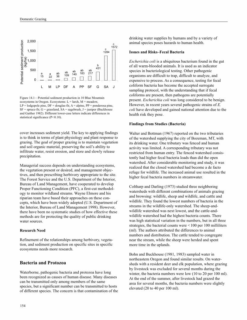
154
Figure 14.1—Potential sediment production in 10 Blue Mountain
ecosystems in Oregon. Ecosystems: L = larch, M = meadow,
LP = lodgepole pine, DF = douglas-fir, A = alpine, PP = ponderosa pine,
SF = spruce-fir, G = grassland, SA = sagebrush, J = juniper (Buckhouse
and Gaither 1982). Different lower-case letters indicate differences in
statistical significance (P<0.10).
cover increases sediment yield. The key to applying findings
is to think in terms of plant physiology and plant response to
grazing. The goal of proper grazing is to maintain vegetationand soil organic material, preserving the soil’s ability to
infiltrate water, resist erosion, and store and slowly release
precipitation.
Managerial success depends on understanding ecosystems,
the vegetation present or desired, and management objec-tives, and then prescribing herbivory appropriate to the site.
The Forest Service and the U.S. Department of the Interior,
Bureau of Land Management, have cooperated to develop
Proper Functioning Condition (PFC), a first-cut methodol-
ogy to monitor wildland streams. Wayne Elmore and his
riparian team have based their approaches on these con-cepts, which have been widely adopted (U.S. Department of
the Interior, Bureau of Land Management 1998). However,
there have been no systematic studies of how effective these
methods are for protecting the quality of public drinking
water sources.
Research Need
Refinement of the relationships among herbivory, vegeta-
tion, and sediment production on specific sites in specific
ecosystems needs more research.
Bacteria and Protozoa
Waterborne, pathogenic bacteria and protozoa have long
been recognized as causes of human disease. Many diseases
can be transmitted only among members of the samespecies, but a significant number can be transmitted to hosts
of different species. The concern is that contamination of the
drinking water supplies by humans and by a variety of
animal species poses hazards to human health.
Issues and Risks–Fecal Bacteria
Escherichia coli is a ubiquitous bacterium found in the gut
of all warm-blooded animals. It is used as an indicator
species in bacteriological testing. Other pathogenic
organisms are difficult to trap, difficult to analyze, and
expensive to process. As a consequence, testing for fecal
coliform bacteria has become the accepted surrogate
sampling protocol, with the understanding that if fecal
coliforms are present, then pathogens are potentially
present. Escherichia coli was long considered to be benign.
However, in recent years several pathogenic strains of E.
coli have developed and gained national attention due to the
health risk they pose.
Findings from Studies (Bacteria)
Walter and Bottman (1967) reported on the two tributaries
of the watershed supplying the city of Bozeman, MT, with
its drinking water. One tributary was fenced and human
activity was limited. A corresponding tributary was not
restricted from human entry. The fenced watershed consis-
tently had higher fecal bacteria loads than did the open
watershed. After considerable monitoring and study, it was
realized that the closed watershed had become a de facto
refuge for wildlife. The increased animal use resulted in the
higher fecal bacteria numbers in streamwater.
Coltharp and Darling (1973) studied three neighboring
watersheds with different combinations of animals grazing
and browsing: wildlife, sheep and wildlife, and cattle and
wildlife. They found the lowest numbers of bacteria in the
streams in the wildlife-only watershed. The sheep-and-
wildlife watershed was next lowest, and the cattle-and-
wildlife watershed had the highest bacteria counts. There
was high statistical variation in the numbers, but in all three
strategies, the bacterial counts were < 100 per 100 milliliters
(ml). The authors attributed the differences to animal
numbers and distribution. The cattle tended to congregate
near the stream, while the sheep were herded and spent
more time in the uplands.
Bohn and Buckhouse (1981, 1983) sampled water in
northeastern Oregon and found similar results. On water-
sheds with a resident deer and elk population, where grazing
by livestock was excluded for several months during the
winter, the bacteria numbers were low (10 to 20 per 100 ml).
At the end of the summer, after livestock had grazed the
area for several months, the bacteria numbers were slightly
elevated (20 to 40 per 100 ml).
Domestic Grazing
0
500
1,000
1,500
2,000
L M LP DF A PP SF G SA J
Pote
ntial sedim
ent pro
duction
(kg/h
a)
a15
a22
ab36
ab109
ab140
ab183
ab217
b431
c1284
c1572

155
Research in central Oregon studied the fate of the coliform
bacteria (Biskie and others 1988; Larsen and others 1988,
1994; Moore and others 1988; Sherer and others 1992). In
this Great Basin rangeland, they discovered that statistically
only 5 days per year experienced enough precipitation to
produce overland flows. Consequently, the probability of
washing fecal material into streams was relatively low.
Cows defecated approximately 11 times a day, but less than
one of these defecations landed in the stream directly or
within 1 meter of the stream where it might be washed into
the stream. Further experiments were conducted to deter-
mine the fate of bacteria defecated directly into the stream.
Ninety percent of these bacteria precipitated to the stream
bottom and attached to sediments. Sediment samples
collected over the next several weeks showed that 90
percent of the lodged bacteria had died within 40 days
(Biske and others 1988; Larsen and others 1988, 1994;
Moore and others 1988; Sherer and others 1992).
The same team of researchers studied the effect of a
strategically placed watering trough on livestock use of a
flowing stream in both summer and winter (Clawson and
others 1994, Miner and others 1992). When snow covered
the ground, cattle were fed hay, and 95 percent of them used
the ground water-fed trough, as opposed to 5 percent that
used the stream. It is speculated that the warmer ground
water (approximately 50 °F or 10 °C) held much greater
appeal to the cattle than did the 32 °F (0 °C) creek. In the
summer, riparian zones provided lush vegetation, shade, and
water. The trough relieved some impact during the summer,
but not as dramatically as during the winter. In late summer,
when most of the available vegetation near the riparian zone
had been consumed, approximately 25 percent of the
livestock drank from the trough, while the remaining 75
percent preferred the stream.
Findings from Studies (Protozoa)
Giardia and Cryptosporidium have drawn considerable
attention recently. Both are debilitating to humans and can
be carried by a wide variety of warm-blooded animals from
waterfowl to rodents; from deer, elk, and beaver to livestock
(see appendix B and chapter 15). Both Giardia and
Cryptosporidium have been known for decades, but only
recently have routine testing following gastrointestinal
complaints from citizens been conducted. It is probable that
what is now diagnosed as Cryptosporidium would at an
early time have been seen simply as flu or food poisoning.
Cryptosporidium oocysts have been found in association
with both wild and domestic animals. Calves consistently
shed greater numbers of oocysts than do older animals
(Atwill 1996). Apparently by 4 months of age, calves
develop a resistance and the number of oocysts shed is
dramatically reduced. An alternative to livestock exclusion
from areas where Cryptosporidium may be a concern is to
ensure that livestock grazing the watershed are older than
4 months. The relationship between oocysts and age of wild
animals is unknown and represents a research question.
Reliability and Limitations of Findings
The fecal bacteria research is reliable and has been consis-
tent over time. The Cryptosporidium work, while compel-
ling, is relatively recent.2 Tate and his colleagues at the
University of California, Davis, continue to investigate these
relationships, the biology, and the management of
Cryptosporidium. Conceptually, these experiments were
solid. Site-specific relationships dictate specific biological
responses. However, regional climatic and temperature
differences may influence the range of variability inherent in
these relationships and to date little is known about wild
animals except that they carry the organisms and shed them
in their feces. Water from wildlands including wilderness,
can contain pathogens that cause human disease if the water
is not adequately treated for purification.
Research Needs
Cryptosporidium research is still in its infancy. Further
studies dealing with the origin and fate of the organisms are
needed. Very little is known about pathogenic E. coli in
livestock under range conditions, and further investigation is
needed.
Chemical and Nutrient Impacts
A number of chemical compounds are associated with
sediment transport. Rangelands are sometimes treated with
herbicide or fertilizer compounds, but the primary chemical
or nutrient problems are with phosphate (PO4
+3) and nitrate
(NO3
-1) associated with eroding soils and fecal material.
Issues and Risks
Cycling of phosphate and nitrate are essential to plant
growth. When vegetation is grazed, potential problems exist
where phosphates and nitrates from feces or attached to
Chapter 14
2 Personal communication. 1999. Kenneth Tate, Professor, Department
Agronomy and Range Science, University of California, Davis, CA 95616.

156
erosion particles that find their way to a stream. Excessive
levels of these nutrients in streams can produce algal blooms
and eutrophication. See chapter 2 for discussion of nutrient
impacts on drinking water.
Findings from Studies
Frequently phosphate and nitrate reach streams in associa-
tion with sediments. See chapter 3, which discusses over-
land flow, erosion, and sediment transfer.
When fecal material enters a stream, phosphate and nitrate
concentrations rise, but wetlands can reduce these concen-
trations. On the Wood River system in Oregon, a nutrient
loading was studied on streams originating from the Crater
Lake National Park, traversing national forest, then private
grazing land, and emptying into a lake listed as hypo-
eutrophic. The concern had been that nutrient loading would
be exacerbated when the water flowed through the grazed
land due to fecal contamination. The data did not bear out
this fear. In fact, the phosphate and nitrate levels decreased.3
It was speculated that the wetlands in the system represented
a natural nutrient sink. In wetlands, chemical processes
associated with anaerobic conditions reduced phosphate and
nitrate concentrations. Furthermore, wetland plants take up
nutrients from the aqueous system. If animals eat wetland
vegetation, nutrients are consumed. Thus, these nutrients are
not redistributed back into the water as when the plant
senesces in place and dies. Apparently the livestock grazing
the wetland consumed the vegetation and its nutrients, and
later redistributed the nutrients away from the stream in
their feces. The result was the observed decline in water-
borne nutrient concentrations.
Reliability and Limitations of Findings
The relationship between nutrient loading and sediment is
clear. The relationship between livestock grazing of wet-
lands and the possibility of nutrient loading abatement is not
proven. The relationships among erosion, sedimentation,
and nutrient loading are universal and are bases for erosion
control worldwide. The possibility of using livestock for
biological control of weeds, for improving plant communi-
ties, for promoting species that encourage infiltration and
reduce overland flow, and even for reducing nutrient loading
(Bedell and Borman 1997) are based on solid research and
management experience. These concepts are predicated on
the ability of vegetation and organic material to enhance
infiltration, which reduces overland flows and subsequent
erosion. The concept of using livestock to harvest nutrient-
rich wetland vegetation is logical but not tested.
Research Needs
Further research is needed on the relationships between
livestock harvesting of streamside vegetation and nutrient
loading of streams.
Key Points
In rangeland, grazing can affect drinking water. Water
quality can be protected by nurturing upland and riparian
vegetation, which can increase the soil’s infiltration capacity
and reduce surface runoff. By understanding the relation-
ships between plant physiology and animal herbivory, one
can tailor grazing practices to enhance infiltration. Both
timing and intensity of grazing must be managed. Increased
infiltration reduces sediment yield, bacterial counts, nutrient
concentrations, and water temperatures. Published data
clearly indicate that improper, abusive grazing can degrade
the quality of public drinking water sources. It is also clear
that proper, prescriptive grazing can produce positive
environmental benefits, and research is needed to develop
and test methods to accomplish them.
Literature Cited
Atwill, E.R. 1996. Assessing the link between rangeland cattle and
waterborne Cryptosporidium parvum infection in humans. Rangelands.
18: 48–51.
Bedell, T.E.; Borman, M.M. 1997. Watershed management guide for the
interior Northwest. Ext. Man. 8436. Corvallis, OR: Oregon State
University Extension Service. 84 p.
Biskie, H.A.; Sherer, B.M.; Moore, J.A. [and others]. 1988. Fate of
organisms from manure point loading into a rangeland stream. Pap.
88–2081. American Society of Agricultural Engineers: 1–14.
Bohn, C.C.; Buckhouse, J.C. 1981. Interpreting coliform counts in
northeast Oregon rangeland streams. Spec. Prog. Rep. 620. Research in
rangeland management. Corvallis, OR: Oregon State University,
Agricultural Experiment Station: 15–17.
Bohn, C.C.; Buckhouse, J.C. 1985. Coliforms as an indicator of water
quality in wildland streams. Journal of Soil and Water Conservation.
40: 95–97.
Buckhouse, J.C.; Bohn, C.C. 1983. Response of coliform bacteria
concentration to grazing management. Spec. Prog. Rep. 682. Corvallis,
OR: Oregon State University, Agricultural Experiment Station: 1–8.
Domestic Grazing
3 Personal communication. 1997. Ronald Hathaway and Rodney Todd,Extension Agents, Klamath County Extension Office, Klamath Falls, OR97601.

157
Buckhouse, J.C.; Bunch, T.E. 1985. Riparian erosion inside and outside
of exclosures on Mill and McKay Creeks: a validation of management.
Spec. Prog. Rep. 743. Research in range management. Corvallis, OR:
Oregon State University, Agricultural Experiment Station: 29–30.
Buckhouse, J.C.; Elmore, W. 1997. Grazing practice relationships:
predicting riparian vegetation response from stream systems. In: Bedell,
T.E.; Borman, M.M., eds. Watershed management guide for the interior
Northwest. Ext. Man. 8436. Corvallis, OR: Oregon State University,
Extension Service: 47–52.
Buckhouse, J.C.; Gaither, R.E. 1982. Potential sediment production
within various vegetative communities found in the Blue Mountains of
Oregon. Journal of Soil and Water Conservation. 37: 120–122.
Buckhouse, J.C.; Knight, R.W.; Skovlin, J.M. 1981. Streambank erosion
and ungulate grazing relationships. Journal of Range Management. 34:
339–340.
Buckhouse, J.C.; Mattison, J.L. 1980. Potential soil erosion of selected
habitat types of the high desert region of central Oregon. Journal of
Range Management. 33: 282–286.
Clawson, J.; Buckhouse, J.C.; Miner, J.R.; Moore, J.A. 1994. An
evaluation of off-site water development and fence configurations
designed to ameliorate water quality impacts by livestock [Abstract].
Corvallis, OR: Oregon State University, Oregon Academy of Science.
1 p.
Coltharp, G.B.; Darling, L.A. 1973. Livestock grazing—a nonpoint
source of water pollution in rural areas? In: Proceedings of the
symposium on rural environmental engineering; 1973 September 15;
Minneapolis. Burlington, VT: University of Vermont. 15 p.
Holechek, J.L.; Piefer, R.D.; Herbel, C.H. 1989. Range management
principles and practices. Englewood Cliffs, NJ: Prentice-Hall. 501 p.
Larsen, R.E.; Buckhouse, J.C.; Moore, J.A.; Miner, J.R. 1988.
Rangeland cattle and manure placement: a link to water quality.
Proceedings of the Oregon academy of science; 1988 February 28;
Corvallis, OR. Corvallis, OR: Oregon State University. 24: 7–15.
Larsen, R.E., Miner, J.R.; Buckhouse, J.C.; Moore, J.A. 1994. Water
quality benefits of having cattle manure deposited away from streams.
Bioresource Technology. 48: 113–118.
Miner, J.R.; Buckhouse, J.C.; Moore, J.A. 1992. Will a water trough
reduce the amount of time hay-fed livestock spend in the stream (and
therefore improve water quality)? Rangelands. 14: 35–38.
Moore, J.A.; Buckhouse, J.C.; Miner, J.R. 1988. Water quality impacts
of alternate rangeland management systems. Comp. Rep. 85–CSRS–2–
2718. [Location of publisher unknown]: U.S. Department of Agriculture,
Cooperative State Research Service. 125 p.
Odum, E.P. 1971. Fundamentals of ecology. Philadelphia: W.B. Saunders
Co. 574 p.
Sherer, B.M.; Miner, J.R.; Moore, J.A.; Buckhouse, J.C. 1988.
Resuspending organisms from a rangeland stream bottom. Transactions
of the American Society of Agricultural Engineers. 31: 1217–1222.
Sherer, B.M.; Miner, J.R.; Moore, J.A.; Buckhouse, J.C. 1992. Indicator
bacterial survival in stream sediments. Journal of Environmental Quality.
21: 591–595.
Skovlin, J.M. 1984. Impacts on wetlands and riparian habitat: a review of
our knowledge. In: Developing strategies for rangeland management. A
report prepared by the Committee on Developing Strategies for
Rangeland Management, National Research Council, National Academy
of Sciences. Boulder, CO: Westview Press: 1001–1104.
Stoddart, L.A.; Smith, A.D.; Box, T.W. 1975. Range management. New
York: McGraw-Hill, Inc. 532 p.
Stringham, T.K.; Buckhouse, J.C.; Krueger, W.C. 1998. Stream
temperatures as related to subsurface waterflows originating from
irrigation. Journal of Range Management. 51: 88–90.
U.S. Department of the Interior, Bureau of Land Management. 1993.
Riparian area management: process for assessing proper functioning
condition. Tech. Ref. 1737–9. Denver: Bureau of Land Management
Service Center. 51 p.
U.S. Department of the Interior, Bureau of Land Management. 1998.
Riparian area management: a user guide to assessing proper functioning
condition and supporting science for lotic areas. Tech. Ref. 1737–15.
Denver: National Applied Resource Sciences Center. 127 p.
Walter, W.G.; Bottman, R.P. 1967. Microbiological and chemical studies
of an open and a closed watershed. Journal of Environmental Health. 30:
157–163.
Chapter 14

158
Chapter 15
Wildlife
Arthur R. Tiedemann1
Introduction
Numbers of large herbivores—mainly deer and elk—are
increasing throughout the United States (Riggs and others,
in press) with a commensurate increase in potential for them
to have an effect on the quality of drinking water sources. In
general, activities that provide healthy habitat usually help
maintain—or at least do not significantly degrade—water
quantity and quality for domestic use. However, contamina-
tion of surface waters by wild herbivores and disease-
organism transmission among domestic herbivores and
wide-ranging large herbivores are major issues that must be
addressed by land managers. Emphasis of this chapter is the
role of large, wild herbivores, such as deer, elk, and moose
on microbiological quality of wildland surface water.
Information is also provided on the role of beavers and
muskrats.
Issues and Risks
Presence of disease-causing organisms in wildland surface
waters is the most critical aspect of problems related to the
influence of wildlife on water quality. There is no doubt that
the human pathogens Giardia spp. and Cryptosporidium
spp. (appendix D), and pathogenic Escherichia coli (E. coli)
are carried by and can be spread by a wide variety of
wildlife.
The impact of large, wild herbivores, such as deer, elk, and
moose, on water quality is an elusive and difficult problem.
These animals range widely and unpredictably, and their
densities and movements relative to surface waters are very
difficult to quantify.
Presence and numbers of fecal coliform (FC) in a given
volume of streamwater [usually number per 100 milliliters
(ml)] are used as indicators of the potential for presence of
disease organisms. At FC counts between 1 and 200 per 100
ml of water, the percentage occurrence of salmonella disease
organisms is 28 percent (Geldreich 1970). Occurrence of
salmonella increases to 85 percent for FC counts of 200 to
2,000 per 100 ml of streamwater and to 98 percent at FC
levels in excess of 2,000 per 100 ml. Bohn and Buckhouse
(1985) comprehensively reviewed the use of FC as an
indicator of wildland water quality. Use of FC counts as an
indicator of disease bacteria has several drawbacks. For
example, it is not a satisfactory indicator for Giardia.
Fecal streptococcus (FS) counts are also used as indicators
of the presence of disease organisms in water (Sinton and
others 1993), but there are no established standards as there
are with FC.
The ratio of FC to FS is one measure of the source of
bacterial contamination of wildland surface water
(Geldreich 1967). Geldreich (1976), Geldreich and Kenner
(1969), and Van Donsel and Geldreich (1971) established
ranges of FC to FS—in feces for humans, > 4; cattle, 1.2 to
0.8; cattle and wildlife mixed, 0.08 to 0.04; and wildlife,
< 0.04. Tiedemann and Higgins (1989) and Tiedemann and
others (1988) applied the concept to wildland watersheds
where several watersheds received only wildlife use and
others received varying degrees of cattle use and wildlife
use. For watersheds with no cattle use, the FC to FS ratio
was < 0.04 for 90 percent of the samples collected. On
watersheds with intensive cattle use of 7 acres [2.8 hectares
(ha)] per animal unit month (aum), the FC to FS ratio in 75
percent of the samples was between 1.2 and 0.8. On
watersheds with lower intensities of cattle use [19 to 20
acres (7.7 to 8.1 ha) per aum], the ratio suggested a mixture
of cattle and wildlife use. Thus, the ratio established by
Geldreich appears to have potential as a tool to separate
wildlife and cattle sources of pollution. Baxter-Potter and
Gilliland (1988) also concluded that the ratio was useful for
distinguishing contaminant sources if the pollution had not
aged in the stream.
Recent efforts have focused on determination of the pres-
ence and sources of actual disease organisms in surface
water. Outbreaks of severe, bloody diarrhea associated with
E. coli [O antigen 157 and H antigen 7 (O157:H7)]
(Armstrong and others 1996) and numerous reports of
Giardia infection (Moore and others 1993) have been
1 Scientist Emeritus, USDA Forest Service, Pacific Northwest ResearchStation, Wenatchee, WA.

159
responsible for emphasis on these organisms. Most cases of
E. coli O157:H7 infection and death have been caused by
consumption of infected meat (Armstrong and others 1996),
including deer jerky (Keene and others 1997). However,
multiple illnesses and deaths have occurred as a result of
drinking contaminated municipal water (Swerdlow and
others 1992). In the case of E. coli, until 1982, this organism
had not been considered a disease-causing entity (Riley and
others 1983, Wells and others 1983). As discussed previ-
ously, E. coli was formerly considered to be benign and an
indicator organism for the presence of organisms that
actually cause diseases.
Severe illness and deaths resulting from E. coli O157:H7
have prompted accelerated research to determine presence
and quantities occurring in various animal species including
wildlife. This is usually done by culture of samples of fresh
fecal material (Atwill and others 1997, Goodrich and others
1973, Monzingo and Hibler 1987), entrail samples from
harvested animals (Atwill and others 1997, Frost and others
1980), or samples from live animals (Erlandsen and others
1990). Transmission among domestic and wildlife species
(especially those with wide ranges) is a crucial facet of this
problem with far-reaching implications for drinking water
quality. Large herbivores, such as deer, elk, and moose, are
without boundaries and may serve as a vector for transmis-
sion of disease organisms among domestic livestock in
pastures or on rangelands. This concern is reinforced by
results of Sargeant and others (1999), who found similar
genetic strains of E. coli O157:H7 in cattle and free-ranging
white-tailed deer sharing the same pasture. Both types of
animals serve as reservoirs for E. coli O157:H7. Although
their conclusions were directed at consumption of deer
meat, their results suggest that we should be alert to poten-
tial problems with the quality of surface drinking water
sources.
Free-ranging white-tailed deer have also been shown to be
potential sources of contamination of Giardia and C.
parvum (Rickard and others 1999). These authors concluded
“the abundance of water throughout the State (Mississippi)
coupled with an overpopulation of white-tailed deer
indicates this cervid may pose a threat to surface water of
this area.”
Relations among wild herbivores and water quality are
highly complex involving the physical and vegetal nature of
the landscape, characteristics of surface water, the species of
wildlife, interrelations among wildlife and domestic
animals, and the disease or indicator organism involved.
Land management activities that tend to concentrate wildlife
or result in increased densities also will influence water
quality. Landscape characteristics that would tend to
influence the effect of wild herbivores on water quality
would be those that encourage or discourage high animal
concentrations near surface water, such as extremely steep
terrain or very dense vegetation. Stream characteristics that
influence organism concentrations are discharge, turbidity,
conductivity, pH, and temperature. Diurnal fluctuations of
bacterial counts are related to discharge, but evidence is
contradictory. Bohn and Buckhouse (1985) provide detailed
analyses of watershed characteristics that influence FC
numbers in streamwater. According to these authors,
bacterial counts generally increase with increasing dis-
charge. Increased counts are apparently the result of
increased flushing of streambanks and associated fecal
deposits. Sediment transport and associated organisms may
also account for some of the increase in counts with
increasing discharge. Counts of FC have been shown to be
much higher in sediments than in surface water (Skinner and
others 1984, Stephenson and Rychert 1982). Counts of FC
seem to be inversely related to stream temperature
(Geldreich and Kenner 1969). Extremes of pH also influ-
ence FC viability with 5.5 to 7.5 as an optimal range
(McFeters and Stuart 1972). Type of wildlife species present
is a major determinant of the type and number of disease
organisms present in surface water. Wildlife closely associ-
ated with water, such as beavers and muskrats, may cause a
protracted, relatively stable contamination problem that may
be fairly predictable. Contamination by wider ranging
wildlife, such as deer and elk, will likely be transient,
sporadic, and somewhat unpredictable. Type of organism
present also depends to some degree on the species of
wildlife present. Giardia, for example, appears to be more
closely tied to presence of water-associated wildlife, such as
beavers and muskrats, than deer and elk (Monzingo and
Hibler 1987). This does not exclude deer and elk as an
element of the cycle of the organism or as a transmission
mechanism. The disease-causing organism E. coli O157:H7
appears to be more closely related to ruminants than to
animals with simple stomachs (Armstrong and others 1996).
Persistence of fecal organisms in surface water is an
important consideration. In the case of domestic animals,
FC levels in streamwater remain high for many months after
cattle are removed (Jawson and others 1982, Tiedemann and
others 1987). We don’t know if the same is true for wildlife
effects on water quality. Fecal coliform do survive for long
periods—at least 1 year in feces of both domestic (Clemm
1977) and wild herbivores (Goodrich and others 1973).
Complexity also arises from the rigorous sample collection,
transport, and analytical procedures that must be followed to
obtain accurate results. Isolation of actual disease organisms
is a complicated laboratory procedure that may also be very
costly. Sampling schedules must be carefully adhered to.
Chapter 15

160
Wildlife
Land treatment measures such as forest thinning, prescribed
burning, shrub control, seeding, and fertilization have the
potential to alter wild herbivore-use patterns. Some treat-
ments, such as prescribed burning, are done to improve
wildlife habitat. These treatments have direct effects on
water quality that are discussed in chapters 10, 12, and 14 of
this report. Because the treatments have the potential to also
alter wild herbivore-use patterns, there is a potential for
indirect effects on water quality. If these habitat modifica-
tions concentrate animals near streams and near domestic
water supply withdrawals, water-quality impacts could be
serious. However, information is lacking on effects of wild
herbivores on water quality associated with changes in
habitat and resultant alterations in herbivore-use patterns.
Findings from Studies
Very little research has been conducted on large, wild
herbivores or beavers and muskrats as the identifiable
sources of fecal contamination of wildland surface water.
Results of studies of maximum levels of FC and Giardia
resulting from wild herbivore use are portrayed in table
15.1. Walter and Bottman (1967) provide some of the
earliest information on effects of wild herbivores on water
quality. They studied FC counts in two watersheds that serve
as a source of municipal water for Bozeman, MT. One
watershed was used by recreationists; the other was fenced
and patrolled to exclude the public and livestock. Thus, the
only potential source of FC in the closed watershed was
wildlife. Deer, elk, and moose were present in the closed
watershed in undetermined numbers. They found maximum
FC counts exceeding 200 per 100 ml of streamwater in the
closed watershed. Fecal coliform counts were actually much
higher in streamwater in the closed than in the open water-
shed, suggesting higher wildlife populations in the closed
watershed—perhaps as a result of high levels of human use
of the open watershed or watershed characteristics.
In another early study, Kunkle and Meiman (1967) mea-
sured maximum FC counts of 25 per 100 ml in streamwater
from an area essentially free from human impact—very
limited hiking or camping, and no domestic livestock
grazing. Wildlife species were not listed, but it is safe to
assume that the area is inhabited by mule deer.
Maximum FC (100+ per milliliter) and Giardia (1 per 100
ml) levels were also high in streamflow from a pristine,
forested watershed in western Washington. These levels
were presumably from wildlife contamination because
human use was very light [5 to 30 days per year per
0.6 miles (1 kilometer) of stream]. Deer, elk, beavers,
mountain beavers, river otters, and marmots were listed as
possible sources of contamination.
Streamwater from pristine land in southern Finland was
shown to contain high levels of FC (maximum, 268 per 100
ml of streamwater). The high counts apparently resulted
from wild deer and moose use of the watershed (Niemi and
Niemi 1991).
In eastern Oregon, forested watersheds that supported no
domestic grazing had maximum FC counts in excess of 500
per 100 ml of streamwater (Tiedemann and others 1987).
Deer and elk were the predominant large herbivores
inhabiting the watersheds.
Maximum Giardia count observed by Monzingo and Hibler
(1987) was 0.06 per 100 ml of streamwater in beaver ponds
in Colorado.
Streamflow from watersheds without domestic livestock in
Utah (Doty and Hookano 1974) and Wyoming (Skinner and
others 1974) contained relatively high counts of FC—22 to
183 per 100 ml. Although FC origin was attributed to
wildlife in both studies, there was no mention of which
wildlife species were responsible. Recreational use in the
two studies was limited to hiking.
Reliability and Limitation of Findings
Research to date lacks replication or detailed examination of
species responsible, numbers of each species, and their
distribution. Its results, however, indicate that wild herbi-
vores pose a risk to drinking water quality.
Studies spanned a relatively broad geographical scope and
suggest that drinking water quality may be a problem
wherever there is contact between wild herbivores and
surface water.
Changes in habitat, whether deliberate or uncontrolled, that
attract wildlife to surface drinking water sources may
increase the risk of introducing contaminants. Management
that discourages animals from concentrating near streams
that are sources of public drinking water may help alleviate
potential contamination problems.

161
Table 15.1—Streamwater fecal coliform and Giardia responses to herbivore use
Maximum counts observeda
Location Setting Herbivore Fecal coliform Giardia spp.b Reference
Colorado Beaver ponds Beaver Not measured 0.021 Monzingo and Hibler 1987
Washington Pristine forested Beaver, 100+ 1 Ongerth and others 1995
watershed, low- mountain
level human use beaver, otter,
marmot
Southern
Finland Pristine lands Elk, deer 268 Niemi and Niemi 1991
Eastern Forested Deer, elk 500+ Tiedemann and others 1987
Oregon watersheds, no
domestic livestock
use
Montana Municipal Deer, elk 200+ Walter and Bottman 1967
watershed, closed
to public access
Colorado Area essentially Not indicated 25 Kunkle and Meiman 1967
free of human
impact, no domestic
livestock use
Utah Watersheds with Not indicated 36–183 Doty and Hookano 1974
no livestock use
Wyoming Watershed open Not indicated 22 Skinner and others 1974
to hikers, no
livestock use
a Counts per 100 milliliters of streamwater.
b Locations with no data in this column indicate that they were not measured.
Research Needs
1. Carefully controlled experiments are needed to determine
the magnitude of the effect of wild herbivores on micro-
biological water quality. Such research must separate
effects of domestic herbivores and humans from those
that result from wildlife. Research must also document
the species of herbivore, the amount of time that each
spends near surface water, and organisms associated with
fecal deposits. Carefully designed water sampling
procedures must accompany these studies. Samples
above, within, and below areas of activity of sufficient
frequency to represent all hydrograph stages will be
essential.
2. Landscape-scale satellite animal tracking experiments
with large, wild herbivores, such as the Starkey Experi-
mental Forest and Range studies in northeast Oregon
(U.S. Department of Agriculture, Forest Service, Pacific
Northwest Research Station, La Grande, OR), provide
opportunities to relate large herbivore movements by
species to changes in water quality. Rationale and
methodology of those studies could be used as a model
for design of water-quality studies. Starkey’s studies
(Rowland and others 1997) could also serve as a model
for research to determine relations among forest and
rangeland treatments, wild herbivore-use patterns, and
resultant changes in water quality.
Chapter 15

162
Wildlife
3. Perhaps it would be appropriate to explore advanced
technology to discourage large, wild herbivores, such as
the technique described by Tiedemann and others (1999)
for cattle. This technique would probably be appropriate
primarily where wild herbivore contamination of surface
water creates severe risks from drinking the water.
4. The literature shows that microbiological and epidemio-
logical research on Giardia and E. coli O157:H7 is well
underway. Hancock and others (1998), however, pose
some problems that are urgently in need of resolution; E.
coli O157:H7 may: (1) have multiple species in which it
resides for long periods; (2) be capable of transiently
colonizing many species; and (3) have an environmental
source, such as sediments where it may be able to
multiply prolifically. Similar questions should be raised
with regard to Giardia.
Key Points
1. Presence of wild herbivores has the potential to influence
microbiological quality of wildland surface water and to
render it unsafe for drinking unless it is adequately
purified. It is important for wildland managers to under-
stand the potential for a problem to exist even though
they cannot document the actual source of contamination.
2. Relationships between wild herbivores and water quality
are highly complex involving physical and vegetal
landscape characteristics, hydrologic parameters (dis-
charge, pH, temperature), type of contaminating organ-
isms, species and numbers of animals, use patterns of
animals, mixing of domestic and wild herbivores, length
of time since animals were present, and land treatment
measures that have been implemented.
3. Potential for presence of disease organisms such as
pathogenic E. coli O157:H7 and Giardia emphasizes the
urgency to understand the relations between wild
herbivores and water quality. No studies have related
water quality to wild herbivore species, numbers, and
land-use patterns.
4. Land treatment measures such as thinning, prescribed
burning, seeding, and fertilization, whether designed
specifically for wildlife habitat alteration or other
management purposes may alter herbivore-use patterns
and exert secondary effects on water quality. These
effects are presently undocumented and poorly under-
stood.
5. Free-ranging large, wild herbivores may be vectors for
transmission of disease organisms among domestic
livestock. Associated contamination of surface water and
potential public health hazards create an urgency to
understand these relations and effects on water quality.
Literature Cited
Armstrong, Gregory L.; Hollingsworth, Jill; Morris, J. Glenn, Jr. 1996.
Emerging foodborne pathogens: Escherichia coli O157:H7 as a model of
entry of a new pathogen into the food supply of the developed world.
Epidemiological Reviews. 18: 29–51.
Atwill, Edward R.; Sweitzer, Richard A.; Das Gracas, C. [and others].
1997. Prevalence of and associated risk factors for shedding
Cryptosporidium parvum oocysts and Giardia cysts within feral pig
populations in California. Applied and Environmental Microbiology. 63:
3946–3949.
Baxter-Potter, Wanda R.; Gilliland, Martha W. 1988. Bacterial pollution
in runoff from agricultural lands. Journal of Environmental Quality. 17:
27–34.
Bohn, Carolyn C.; Buckhouse, John C. 1985. Coliforms as an indicator
of water quality in wildland streams. Journal of Soil and Water
Conservation. January-February: 95–97.
Clemm, David. 1977. Survival of bovine enteric bacteria in forest streams
and animal wastes. Ellensburg, WA: Central Washington University.
20 p. M.S. thesis.
Doty, R.D.; Hookano, E., Jr. 1974. Water quality of three small water-
sheds in northern Utah. Res. Note INT–186. Ogden, UT: U.S. Depart-
ment of Agriculture, Forest Service, Intermountain Forest and Range
Experiment Station. 6 p.
Erlandsen, S.L.; Sherlock, L.A.; Bemrick, W.J. [and others]. 1990.
Prevalence of Giardia spp. in beaver and muskrat populations in
northeastern States and Minnesota: detection of intestinal trophozoites at
necropsy provides greater sensitivity than detection of cysts in fecal
samples. Applied and Environmental Microbiology. 56: 31–36.
Frost, F.; Plan, B.; Leitchy, B. 1980. Giardia prevalence in commercially
trapped mammals. Journal of Environmental Health. 42: 245–249.
Geldreich, E.E. 1967. Fecal coliform concepts in stream pollution. Water
Sewage Works. 114: R–98 and R–107 to R–110.
Geldreich, E.E. 1970. Applying bacteriological parameters to recreational
water quality. Journal of the American Water Works Association. 62:
113–120.
Geldreich, E.E. 1976. Fecal coliform and fecal streptococcus density
relationships in waste discharges and receiving waters. Critical Reviews
in Environmental Control. 6: 349–369.
Geldreich, E.E.; Kenner, B.A. 1969. Concepts of fecal streptococci in
stream pollution. Journal of Water Pollution Control Federation. 41:
R336–R352.
Goodrich, Thomas D.; Stuart, David G.; Walter, William G. 1973.
Enteric bacteria found in elk droppings in a municipal watershed in
Montana. Journal of Environmental Health. 34: 375–377.
Hancock, Dale D.; Besser, Thomas E.; Rice, Daniel H. [and others].
1998. Multiple sources of Escherichia coli O157 in feedlots and dairy
farms in the Northwestern U.S.A. Preventive Veterinary Medicine. 35:
11–19.

163
Jawson, M.D.; Elliott, L.F.; Saxton, K.E.; Fortier, D.H. 1982. The effect
of cattle grazing on indicator bacteria in runoff from a Pacific Northwest
watershed. Journal of Environmental Quality. 11: 621–627.
Keene, William E.; Sazie, Elizabeth; Kok, Janet [and others]. 1997. An
outbreak of Escherichia coli O157:H7 infections traced to jerky made
from deer meat. Journal of the American Medical Association. 277:
1229–1231.
Kunkle, Samuel H.; Meiman, James R. 1967. Water quality of mountain
watersheds. Hydrol. Pap. 21. Ft. Collins, CO: Colorado State University.
52 p.
McFeters, G.A.; Stuart, D.G. 1972. Survival of fecal coliform bacteria in
natural waters: field and laboratory studies with membrane-filter
chambers. Applied Microbiology. 24: 805–811.
Monzingo, D.L., Jr.; Hibler, C.P. 1987. Prevalence of Giardia sp. in a
beaver colony and the resulting environmental contamination. Journal of
Wildlife Diseases. 23: 576–585.
Moore, A.C.; Herwaldt, B.L.; Craun, G.F. [and others]. 1993.
Surveillance for waterborne disease outbreaks—United States
1991–1992. Morbidity and Mortality Weekly Report. 42(SS–5): 1–22.
Niemi, R.M.; Niemi, J.S. 1991. Bacterial pollution of waters in pristine
and agricultural lands. Journal of Environmental Quality. 20: 620–627.
Ongerth, J.E.; Hunter, G.D.; DeWalle, F.B. 1995. Watershed use and
Giardia cyst presence. Water Research. 29: 1295–1299.
Rickard, Lora G.; Siefker, Carla; Boyle, Carolyn R.; Gentz, Edward J.
1999. The prevalence of Cryptosporidium and Giardia spp. in fecal
samples from free-ranging white-tailed deer (Odocoileus virginianus) in
the Southeastern United States. Journal of Veterinary Diagnostic
Investigation. 11: 65–72.
Riggs, R.A.; Tiedemann, A.R.; Cook, J.G. [and others]. [In press].
Modification of mixed-conifer forests by ruminant herbivores in the
Blue Mountains ecological province. Res. Pap. Portland OR: U.S.
Department of Agriculture, Forest Service, Pacific Northwest Research
Station.
Riley, L.W.; Remis, R.S.; Helgerson, S.D. [and others]. 1983. Hemor-
rhagic colitis associated with a rare Escherichia coli serotype. New
England Journal of Medicine. 308: 681–685.
Rowland, M.M.; Bryant, L.D.; Johnson, B.K. [and others]. 1997. The
Starkey project: history, facilities, and data collection methods for ungu-
late research. Gen. Tech. Rep. PNW–396: Portland, OR: U.S. Department
of Agriculture, Forest Service, Pacific Northwest Research Station. 62 p.
Sargeant, Jon M.; Hafer, Dale J.; Gillespie, Jerry R. [and others]. 1999.
Prevalence of Escherichia coli O157:H7 in white-tailed deer sharing
rangeland with cattle. Journal of the American Veterinary Medical
Association. 215: 792–794.
Sinton, L.W.; Donnison, A.M.; Hastie, C.M. 1993. Faecal streptococci as
faecal pollution indicators: a review. 1: Taxonomy and enumeration.
New Zealand Journal of Marine and Freshwater Research. 27: 101–115.
Skinner, Quentin D.; Adams, John C.; Rechard, Paul A.; Beetle, Allen
A. 1974. Effect of summer use of a mountain watershed on bacterial
water quality. Journal of Environmental Quality. 3: 329–335.
Skinner, Quentin D.; Speck, John E., Jr.; Smith, Michael; Adams, John
C. 1984. Stream water quality as influenced by beaver within grazing
systems in Wyoming. Journal of Range Management. 37: 142–146.
Stephenson, G.R.; Rychert, R.C. 1982. Bottom sediment: a reservoir of
Escherichia coli in rangeland streams. Journal of Range Management.
35: 119–123.
Swerdlow, D.L.; Woodruff, B.A.; Brady, R.C. [and others]. 1992. A
waterborne outbreak in Missouri of Escherichia coli O157:H7 associated
with bloody diarrhea and death. Annals of Internal Medicine. 117:
812–819.
Tiedemann, A.R.; Higgins, D.A. 1989. Effects of management strategies
on water resources. In: Quigley, T.M.; Sanderson, H.R.; Tiedemann,
A.R., eds. Managing interior Northwest rangelands: the Oregon range
evaluation project. Gen. Tech. Rep. PNW–238. Portland, OR: U.S.
Department of Agriculture, Forest Service, Pacific Northwest Research
Station: 57–91.
Tiedemann, A.R.; Higgins, D.A.; Quigley, T.M. [and others]. 1987.
Responses of fecal coliform in streamwater to four grazing strategies.
Journal of Range Management. 40: 22–329.
Tiedemann, A.R.; Higgins, D.A.; Quigley, T.M. [and others]. 1988.
Bacterial water quality responses to four grazing strategies—compari-
sons with Oregon standards. Journal of Environmental Quality. 17:
492–498.
Tiedemann, A.R.; Quigley, T.M.; White, L.D. [and others]. 1999.
Electronic (fenceless) control of livestock. Res. Pap. PNW–510.
Portland, OR: U.S. Department of Agriculture, Forest Service, Pacific
Northwest Research Station. 23 p.
Van Donsel, D.J.; Geldreich, E.E. 1971. Relationships of Salmonellae to
fecal coliforms in bottom sediments. Water Resources. 5: 1079–1087.
Walter, William G.; Bottman, Robert P. 1967. Microbiological and
chemical studies of an open and closed watershed. Journal of Environ-
mental Health. 30: 157–163.
Wells, J.G.; Davis, B.R.; Wachsmuth, I.K. [and others]. 1983.
Laboratory investigation of hemorrhagic colitis outbreaks associated
with a rare Escherichia coli serotype. Journal of Clinical Microbiology.
18: 512–520.
Chapter 15
164
Chapter 16
Water Birds
Christopher A. Nadareski1
Introduction
This chapter synthesizes the available information on the
sources, mechanisms, and risks of drinking water contami-
nation from water birds. By water birds, we mean geese,
ducks, and other duck-like swimming birds such as cormo-
rants, gulls, and wading birds. In general, activities that
provide healthy habitat usually help maintain—or at least do
not significantly degrade—water quantity and quality for
domestic use. However, water birds have been implicated in
the contamination of both large and small drinking water
supplies.
Issues and Risks
The U.S. Department of Agriculture, Wildlife Services,
collect and disseminate information about nuisance-related
problems caused by a variety of birds. Birds commonly
create human health concerns by polluting potable drinking
water supplies and fouling recreation areas, such as swim-
ming beaches. Species like the cormorant are thought to
negatively impact recreational fisheries and drinking water
supplies. Some terrestrial bird species, such as swallows,
pigeons, and starlings, may nest, feed, or roost in water
intake structures where their defecation has negative
impacts on water quality. Biological, chemical, and nutrient
pollutants may be released or deposited by water birds. The
type and quantity of pollutant will determine what kind and
level of water bird management is required to prevent
contamination to a reservoir system.
Estimating impacts from the various types of contamination
requires information on the species of water bird inhabiting
the water supply, the number of birds per species, the daily
defecation or pellet regurgitation rates, the amount of
contamination per specified weight of feces or pellet, and
the daily amount of activity by each bird on the water. The
principal pathogens of concern are listed in table 16.1.
Findings from Studies
Studies have found that water birds and some terrestrial
species affect the biological, nutrient, and chemical quality
of water.
Contamination
Biological
Among the various types of water bird contaminants are
excrement containing bacteria, protozoans, or enteric
viruses. These contaminants are routinely monitored by
water suppliers and regulated by the U.S. Environmental
Protection Agency (EPA) and various State health depart-
ments. Numerous studies have documented the occurrence
of fecal coliform bacteria and other pathogens in many
North American water bird species (Ashendorf and others
1997, Gould and Fletcher 1978, Hatch 1996, Hussong and
others 1979). As a result, bird control programs have been
developed and implemented at many municipal water
sources (Ashendorf and others 1997, Blokpoel and Tessier
1984). Water bird excrement has been reported to contain
both human and nonhuman pathogens. Microbiological
analysis for human bacterial pathogens found in drinking
water are generally represented by the fecal coliform
bacteria group which is used as an index to identify the
probability one or more of these organisms will be present
in the sample (chapter 2 and table 16.1). Fecal coliform
originates solely from warm-blooded animals , and analyti-
cal methods to identify the origin of bacterial type (human
versus nonhuman) are currently under investigation. These
new methods require an expensive and time-consuming
examination of the sample. As a result, most public water
suppliers, at best, can only speculate on the origin of the
drinking water bacterial contamination. In the larger
municipal water systems, such as New York City’s, methods
are being developed to link bacterial sources from water
samples to human, nonhuman, or both sources.
1 Research Scientist, New York City Department of EnvironmentalProtection, Valhalla, NY.

165
Table 16.1—Indicator and principal pathogens of concern in contaminated drinking water
Organism type Disease Symptoms
Fecal coliform bacteria group
BacteriaEscherichia coli, Klebsiella Diarrhea, dysentery, Diarrhea, nausea, cramps, fever, vomiting, pneumonae hemorrhagic colitis mucus in stools
Important human pathogenicorganisms suspected from fecesBacteria
Shigella spp. Shigellosis Diarrhea, fever, cramps, tenesmus, blood in stools
Salmonella typhimurium Salmonellosis Abdominal pain, diarrhea, nausea, vomiting, fever
S. typhi Typhoid fever Abdominal pain, fever, chills, diarrhea or constipation, intestinal hemorrhage
Enterotoxigenic Diarrhea Diarrhea, fever, vomiting
Campylobacter jejuni Gastroenteritis Abdominal pain suggesting acute appendicitis, fever, headache, malaise, diarrhea, vomiting
Vibrio cholerae (incidence rareor negligible in the UnitedStates) Gastroenteritis Vomiting, diarrhea, dehydration
Yersinia spp. Plague, hemorrhagic Diarrhea, fever, abdominal pain enterocolitis, terminal ileitis, mesenteric lymphadenitis, septicemia
Enteric virusesHepatitis A virus Hepatitis Fever, malaise, anorexia, jaundice
Norwalk-like agent Gastroenteritis Diarrhea, abdominal cramps, headache, fever, vomiting
Virus-like 27 nm particles Gastroenteritis Vomiting, diarrhea, fever
Rotavirus Gastroenteritis Vomiting followed by diarrhea for 3 to 8 days
ProtozoaGiardia lamblia Giardiasis Chronic diarrhea, abdominal cramps,
flatulence, malodorous stools, fatigue, weight loss
Cryptosporidium Cryptosporidiosis Abdominal pain, anorexia, watery diarrhea, weight loss; immuno-compromised individuals may develop chronic diarrhea
Entamoeba histolytica Amebiasis Vary from mild diarrhea with blood and mucus to acute or fulminating dysentery with fever and chills
nm particles = nanometers.
Source: Murray and others 1995, Hurst and others 1997.
Chapter 16

166
Water Birds
Nutrients
Contributions of nutrients to aquatic ecosystems by water
bird excrement have been well documented (Gould and
Fletcher 1978, Manny 1994), but debate continues over the
significance of impacts from bird defecation on nutrient
loading (Hoyer and Canfield 1994, Murphy 1984). Among
the various nutrients identified in water bird excrement,
nitrogen and phosphorus are of greatest interest. Both have
the potential to increase the rate of eutrophication and
degrade the quality of a drinking water supply
(Vollenweider and Kerekes 1980).
Chemical
Another type of water bird contamination may be of
chemical origin. Glandular releases, body oils, pesticides,
and other hydrocarbons are transported by the birds. The
impact to drinking water supplies from glandular releases
and body oils emitted by water birds is not well understood.
Chemical pollutants carried externally on feathers or
vectored by water birds, although not well documented, may
potentially cause contamination of a water supply. For
example, many reservoir systems do not provide adequate
food supplies for gulls or other opportunistic feeders. Gulls,
therefore, will seek alternative foraging locations, such as
agricultural areas, urban centers, moist fields, and landfills,
where they may be exposed to a variety of chemicals either
through ingestion or external attachment. The gulls may
accumulate various chemicals on their feathers and transport
them back to the reservoir where they roost. Gulls may also
ingest contaminated materials from landfills or sewage
treatment facilities, carry them back to the reservoir, and
regurgitate them. Additional studies are needed to determine
these impacts.
Water Birds as Vectors of Contamination
A variety of human-related activities, such as urbanization,
resource exploitation, agriculture, and land conservation,
have the potential to promote or discourage populations of a
variety of water bird species.
Water birds deposit pollutants in drinking water supplies
during roosting, foraging, and overflights. The birds may
acquire pathogens, such as Giardia spp. or Cryptosporidium
spp., from domestic farm animals (Graczyk and others
1998) and from urban centers such as shopping malls or
landfills. Agricultural operations, such as the spreading of
fodder or manure, growing crops, and tilling soil, offer
attractive foraging locations for some species that travel
great distances. In a study of Canada geese foraging on
agricultural land near the Chesapeake Bay, researchers
identified a high incidence of Giardia and Cryptosporidium
in their fecal matter (Graczyk 1996) compared to an
extremely low incidence of the same two protozoans in
geese sampled at an urban reservoir 15 miles north of New
York City.
The pathways by which water contaminated with biological
materials, chemicals, and nutrients can enter into the
reservoir from water birds include streamflow through
drainage basins, stormwater surface sheet flow, fly-over
fecal releases, and direct fecal deposition. The location of
the source of contamination with respect to a reservoir will
determine the degree of water-quality impacts. Size and
water flow patterns in relation to the water intake structure
from which drinking water is drawn also affects the extent
of impacts. The extent of contamination depends on the die-
off rate, settling rate, and water travel time.
Seasonality of Impacts
Pollutant loadings from water birds vary widely by season.
Migratory birds may cause problems only during brief
stopovers. Local breeding populations of water birds may
also have negative impacts, and those impacts may persist
through much of the year. The location of bird activity
(roosting, breeding, foraging, etc.) on the reservoir relative
to a water intake facility may also determine importance of
strategies for managing water bird populations.
Reliability and Limitations of Findings
The types of water-quality impacts are understood. The
magnitudes of impacts are less well understood. Resident
and migratory water birds will pose similar problems to
water supply reservoirs. The magnitude of the impact will
vary by species and number of birds inhabiting the reservoir,
the surrounding environs and associated sources of contami-
nation, and seasonal patterns of migration. Therefore, water
bird impacts will vary and need to be assessed for each
reservoir.
167
Key Points
1. Land managers may have different objectives concerning
habitat management for water bird species than reservoir
managers. Both forest managers and reservoir managers
can and do influence the population dynamics of water
bird species. Their management objectives can conflict;
for example, the forest manager may want to increase
populations of certain water bird species while the
reservoir manager may try to decrease or eliminate their
activity on or near the reservoir (see New York City case
study).
2. To address the contamination of drinking water supplies
by water birds, a comprehensive watershed protection
plan should be drawn up. This plan needs to identify all
major sources of pollution. If it is determined that water
birds are major contributors, an additional plan for water
bird management should be developed. This water bird
management plan should also incorporate objectives both
for the land manager and the reservoir manager. Popula-
tions of all water bird species that breed or migrate
throughout the watershed should be inventoried to
identify all potential impacts on water quality. The type
of pollution should be identified, as should its potential
origins. Where the source of the contaminant is human
activity and birds are only a vector, it may be possible to
control the contamination by changing the offending
human activity.
Case Study: New York City Waterfowl
Management Program
As the Nation’s largest, unfiltered water supplier, the city of
New York Department of Environmental Protection (DEP)
is responsible for the maintenance of 19 reservoirs, 3
controlled lakes encompassing an area of almost 2,000
square miles, and serving 9 million consumers. Beginning in
the early 1980’s, the city enhanced its water-quality moni-
toring programs to address watershed protection issues. As
more stringent Federal regulations were implemented
through the Safe Drinking Water Act of 1986 and subse-
quent Surface Water Treatment Rule of 1989, New York
City remained determined to maintain its unfiltered status
through stringent criteria set by the EPA. In order to fulfill
this filtration avoidance determination, the DEP developed a
comprehensive Watershed Protection Program (WPP) to
identify and eliminate sources of pollution that would
compromise its water quality. An important component of
the WPP was the implementation of a Waterfowl Manage-
ment Program that identified birds, particularly gulls, geese,
ducks, and cormorants, as the primary source of fecal
coliform bacteria to the water system. Baseline bird
population data was well correlated with the seasonal
elevations of bacteria. As a result, DEP instituted a bird
deterrent/harassment program to eliminate the presence of
both breeding and migratory Canada geese and migratory
gulls, ducks, and other water birds. Techniques used to deter
the birds included shoreline fencing, meadow management
to deter feeding opportunities, bird distress tapes, and the
use of pyrotechnics from motorboats and hovercraft from
dawn to dusk on a daily basis. The techniques were highly
effective: elimination of defecation from roosting birds
eliminated the seasonal elevations of bacteria, allowing New
York City to maintain its filtration avoidance status.
Literature Cited
Ashendorff, A.; Principe, M.A.; Seeley, A. [and others]. 1997. Watershed
protection for New York City’s supply. Journal of the American Water
Works Association. 89(3): 75–88.
Blokpoel, G.; Tessier, G.D. 1984. Overhead wires and monofilament lines
exclude ring-billed gulls from public places. Wildlife Society Bulletin.
12: 55–58.
Gould, D.J.; Fletcher, M.R. 1978. Gull droppings and their effects on
water quality. Water Research. 12: 665–672.
Graczyk, T.K.; Fayer, R.; Trout, J.M. [and others]. 1998. Giardia sp.
cysts and infectious Cryptosporidium parvum oocysts in the feces of
migratory Canada geese (Branta canadensis). Applied and Environmen-
tal Microbiology. 64(7): 2736–2738.
Hatch, Jeremy J. 1996. Threats to public health from gulls (Laridae).
International Journal of Environmental Health Research. 6: 5–16.
Hoyer M.V.; Canfield, D.E. 1994. Bird abundance and species richness on
Florida lakes—influence of trophic status, lake morphology, and aquatic
macrophytes. Hydrobiologia. 280: 107–120.
Hurst, C.J.; Knudsen, G.R.; McIvering, M.J. [and others]. 1997.
Manual of environmental microbiology. Washington, DC: American
Society for Microbiology Press. 894 p.
Hussong, D.; Damare, J.M.; Limpert, R.J. [and others]. 1979. Microbial
impact of Canada geese (Branta canadensis) and whistling swans
(Cygnus columbianus columbianus) on aquatic ecosystems. Applied and
Environmental Microbiology. 37(1): 14–20.
Manny, B.A.; Johnson, W.C.; Wetzel, R.G. 1994. Nutrient additives by
waterfowl to lakes and reservoirs: predicting their effects on productivity
and water quality. Hydrobiologia. 279: 121–132.
Murphy, S.M.; Kessel, B.; Vining, L.J. 1984. Waterfowl populations and
limnological characteristics of taiga ponds. Journal of Wildlife
Management. 48(4): 1156–1163.
Murray, P.R.; Baron, E.J.; Pfaller, M.A. [and others]. 1995. Manual of
clinical microbiology. 6th ed. Washington, DC: American Society for
Microbiology Press. 1,482 p.
Chapter 16

168
New York City Department of Environmental Protection. 1993.
Implications of phosphorus loading for water quality in NYC Reservoirs.
Corona, NY: New York City Department of Environmental Protection.
65 p.
U.S. EPA. 1999. U.S. EPA’s unfiltered water supply systems guidance
manual—revised draft. Washington, DC: U.S. Environmental Protection
Agency. 58 p.
Vollenweider, R.A.; Kerekes, J.J. 1980. Background and summary results
of the OECD cooperative program on eutrophication. EPA 440/5–81–
010:25–36. Washington, DC: Environmental Protection Agency: 25–35.
Water Birds

169
Chapter 17
Fish and Aquatic Organisms
C. Andrew Dolloff 1
Introduction
Freshwater fish management can impact water quality by
manipulating fish and other organisms and by altering the
physical, chemical, or biological attributes of habitat.
Fishery managers manipulate populations for a variety of
reasons, including attempts to maximize yield, control size
and age structure, establish populations of desirable and
remove populations of undesirable species, and to reestab-
lish populations and communities that have been extirpated.
Habitat management often accompanies attempts to manipu-
late populations. All components of habitat are subject to
manipulation, including not only the obvious structural
elements, such as substrate, cover, and flow obstructions,
but also water chemistry and the content of the biological
community.
Fish Hatcheries and Aquaculture Facilities
Issues and Risks
Fish hatcheries or fish culture facilities can reduce water
quality. Untreated effluent from these facilities typically
consists of metabolic waste products and solids derived
from uneaten fish food and fish wastes (Goldburg and
Triplett 1997). In addition, culture facilities also may
intermittently discharge pathogenic bacteria and parasites
and the chemicals and drugs used in the prevention or
treatment of disease (Liao 1970, Piper and others 1986). The
usual waste stream from a culture facility can be treated as a
chronic point source and effluent quality and quantity can be
monitored at or immediately below the outfall. Monitoring
results tend to be highly variable because of variation in
production schedules and other activities (Foy and Rosell
1991) such as periodic cleaning and flushing (Bergheim and
others 1984).
Findings from Studies
The quality of effluent water varies considerably depending
on the specific features of the culture system including the
species of fish, intensity of production, the diet and feeding
regime, and the temperature and chemical character of
source water (Axler and others 1997). The four most
important dissolved constituents of fish cultural wastewater
include ammonia, nitrate, phosphate, and organic matter.
Ammonia is toxic to most aquatic life and all four constitu-
ents are primary agents of eutrophication. Along with
dissolved organic matter, suspended solids, which are
predominantly organic, contribute to biological oxygen
demand in receiving waters. Nutrient loading can be
significant, as 60 to 75 percent of the nitrogen and phospho-
rus in fish food ultimately becomes part of the waste stream
(Axler and others 1997). Unless intakes for domestic water
supplies are located immediately downstream from the
outfall, however, hatchery effluents are not likely to severely
degrade domestic water supplies.
Effluents from trout farms may diminish water quality
slightly during periods of low flow and high temperature
(Selong and Helfrich 1998). In a study of five Virginia trout
farms, Selong and Helfrich (1998) found that total ammonia
nitrogen, un-ionized ammonia nitrogen, and nitrite nitrogen
levels increased downstream from effluent outfalls but did
not exceed thresholds for lethal exposure for aquatic
organisms. Dissolved oxygen levels also decreased but were
typically above 7.0 parts per million (ppm). Temperature,
pH, nitrate nitrogen, and total phosphorus levels did not
differ from upstream levels. Substrate embeddedness was
greater below outfalls from two farms but settleable solids
concentrations were always < 0.1 ppm. The lack of signifi-
cant water-quality degradation reflected the tendency of
growers to adjust production to correspond to periods of
high flow and low-to-moderate temperature (Selong and
Helfrich 1998). In Washington State, however, hatchery
effluents during the summer had significantly elevated
temperature, pH, suspended solids, ammonia, organic
nitrogen, total phosphorus, and biological oxygen demand
(Kendra 1991). Phosphorus loading in hatchery effluent in
one Washington State creek was equivalent to secondarily
treated sewage discharge from a town of 2,300 people. The1 Project Leader, USDA Forest Service, Southern Research Station,Blacksburg, VA.
170
influence of hatchery effluents tends to be localized in the
immediate downstream reach (Doughty and McPhail 1995).
Effects on periphyton and macroinvertebrates were not
detected about 1,200 feet [366 meters (m)] downstream of
the outfalls from five Virginia trout farms (Selong and
Helfrich 1998).
Because most of the total nutrient load produced at a typical
facility is in the form of settleable solids, treatment usually
consists of diverting wastewater through settling basins
before discharge (Piper and others 1986). Much of the
variation observed in effluent waste among facilities can be
traced to differences in settling characteristics (Mudrak
1981). When located near towns or cities, culture facilities
can avoid discharging directly into streams or rivers by
connecting to municipal sewage treatment facilities.
Fish disease organisms, chemicals, and other additives
commonly used in culture facilities also may influence the
quality of water for domestic use. Fish trematodes, cestodes,
and nematodes can be transmitted to people who eat certain
species of raw fish. In general, however, fish diseases do not
present risks to human health (Hoffman 1999). Most
potential problems with fish disease and water quality arise
from the chemicals and procedures used in treatment. At
present, relatively few chemicals have been approved by the
U.S. Food and Drug Administration (FDA) for use in the
treatment of fish diseases. The antibacterials approved for
use on food fishes include oxytetracycline, sulfamethoxine
(Romet), and sulfamerazine. Most drugs are administered
through feed, from which a considerable fraction may be
released into the environment. Release occurs through three
routes: uningested food, feces, and in urine and bile fluid
(Capone and others 1996). Residues of oxytetracycline in
sediments under net pens of intensively cultured (and
treated) Atlantic salmon were present for at least 10 months
after treatment (Capone and others 1996). Other drugs
approved for use in treating fish include formalin (for the
treatment of external parasites and fungus on fish eggs) and
tricaine methanesulfonate, an anesthetic. The FDA also
maintains a list of unapproved new animal drugs (drugs that
have not gone through the formal approval process but are
not expected to have a negative impact on the environment)
for use in aquaculture of food fishes provided the following
conditions are met:
1. The drugs are used for the prescribed indications,
including species and life stage;
2. The drugs are used at the prescribed dosages;
3. The drugs are used according to good management
practices;
4. The product is of an appropriate grade for use in food
animals; and
5. An adverse effect on the environment is unlikely.
Among a host of common compounds and substances in this
classification are sodium chloride and ice. Examples of
unapproved drugs for use in aquaculture are acetic acid
(parasiticide for fish), calcium chloride (ensures proper egg
hardening, aids in maintaining osmotic balance in fish),
carbon dioxide gas (fish anesthetic), hydrogen peroxide
(fungicide), magnesium sulfate (controls monogenetic
trematode and external crustacean infestations), potassium
chloride (relieves osmoregulatory stress and prevents
shock), povidone iodine compounds (fish egg disinfectant),
sodium sulfate (improves egg hatchability), and urea and
tannic acid (denatures adhesive component of fish eggs).
In addition to treating specific diseases, all culture facilities
must undergo periodic cleaning and sterilization. Chlorine
(HTH) is often used for this purpose; exposure to 5 ppm for
1 hour kills nearly everything. Chlorine rapidly loses its
toxicity (1 day or less) and can be neutralized by sodium
thiosulfate.
Reliability and Limitations of Findings
A large body of research has accumulated on the design,
construction, operation, and maintenance of fish culture
facilities. Because a significant portion of this research has
addressed the issue of effluent management, the findings are
considered highly reliable. These findings are widely
applicable to flowing water.
Research Needs
None identified.
Key Points
Existing knowledge will permit managers and policymakers
to make informed decisions about the impact of culture
facilities on domestic water supplies.
Fish and Aquatic Organisms
171
Chemical Reclamation
Issues and Risks
Piscicidal (fish-killing) compounds have been used to
sample, control, or eradicate fish populations since the
1930’s (Bettoli and Maceina 1996). Purposes have included
eradication of exotic species such as common carp from
ponds, lakes, and reservoirs and removal of nonnative
species from headwater streams. With the exception of
sampling programs, the objective of most piscicide applica-
tions is to remove one or more species so that the water
body can be stocked soon after poisoning with species
considered more desirable.
Findings from Studies
Only registered piscicides may be applied to water in North
America. Among a variety of possible compounds, only
rotenone (trade name Noxfish), antimycin A (trade name
Fintrol), 3-trifluoromethyl-4-nitrophenol (TFM), and
Bayluscide (a nitosalicylanilide salt, trade name Bayer 73)
are approved for use in the United States. Bayluscide and
TFM, either alone or in combination, are used exclusively to
sample or control sea lamprey, primarily in streams flowing
into the Great Lakes (Bettoli and Maceina 1996, Marking
1992). In the United States, lampricides can be applied only
by personnel certified by the U.S. Fish and Wildlife Service
or an approved State conservation agency (Bettoli and
Maceina 1996).
Rotenone, a naturally occurring chemical derived from
the roots of tropical plants in the genera Derris and
Lonchocarpus, has been used for centuries by native people
to kill fish for food. Rotenone is highly toxic to fish, which
are killed by disruptions in cellular respiration (Haley 1978).
Most nontarget aquatic organisms usually are not affected
by the concentrations of rotenone used to kill fish, but high
doses can kill amphibians, some reptile species, and a
variety of macroinvertebrates (Bettoli and Maceina 1996).
The toxicity and persistence of rotenone are influenced by
turbidity, temperature, and pH; in general, rotenone is most
toxic in clear, warm, acidic water. Residues of rotenone
were detectable in the bottom sediments of experimental
ponds in Wisconsin for nearly 14 days during the spring at
46 oF (8 oC), but decreased below the limits of detection
within 3 days during the summer at 72 oF (22 oC) and during
the fall at 59 oF (15 oC) (Dawson and others 1991). Higher
temperatures coupled with the presence of clay (bentonite)
led to adsorption and rapid decline in residues. Dawson and
others (1991) suggested that at warmer temperatures, water
treated with rotenone would be safe for swimming immedi-
ately after treatment with a concentration of 250 parts per
billion (ppb). A strong oxidizing agent such as potassium
permanganate (applied at 2.0 to 2.5 ppm) will detoxify
rotenone when applied downstream of treatment sections in
flowing water or in lakes where managers wish to limit the
area of kill.
Rotenone has a low mammalian toxicity (Marking 1988)
and relatively short half-life (< 1 day in water at 73 oF)
(Gilderhus and others 1988). Nevertheless, negative public
perceptions about the use of any poisonous substance in
open water have curtailed the use of rotenone over the last
decade. Older formulations of rotenone, no longer approved
for sale in the United States, sometimes contained carrier
substances such as trichloroethylene and piperonyl butoxide,
which are known carcinogens. Residues of the latter were
detected up to 9 months after treatment of Lake Davis in
California and caused disruption of a public drinking water
supply that drew national publicity.
Similar to rotenone, antimycin is relatively nontoxic to
mammals (Herr and others 1967) but highly poisonous to
fish. Antimycin toxicity in water varies by species, and
concentrations over 100 ppb may be required to kill resistant
species (Bettoli and Maceina 1996). The effectiveness of
antimycin may decrease below 50 oF (10 oC) (Tiffan and
Bergersen 1996), but in warm water, temperature does not
greatly influence its toxicity. High turbidity (Gilderhus
1982) and alkalinity (Tiffan and Bergersen 1996) decrease
its effectiveness and persistence (Bettoli and Maceina 1996,
Lee and others 1971). Turbulence leading to oxidation and
foaming also may contribute to antimycin inactivation
(Tiffan and Bergersen 1996).
Reliability and Limitations of Findings
A large body of research has accumulated on the short- and
long-term effects of chemical reclamation. Studies have
been conducted in both warmwater and coldwater habitats
under widely varying conditions. The findings are consid-
ered highly reliable and widely applicable.
Research Needs
None identified.
Key Points
Existing knowledge will permit managers and policymakers
to estimate impacts of piscicides on fish populations and
water quality. However, controversy likely will continue
over the use of piscicides in sources of public water
supplies.
Chapter 17

172
Restoration and Reintroduction
of Populations and Communities
Issues and Risks
With the growth in environmental awareness in recent years,
management agencies increasingly are called upon to restore
species that have been intentionally or accidentally extir-
pated from aquatic ecosystems. In most situations, the
impact of the restoration on water quality will be almost
entirely positive because improved water quality is one of
the prerequisites for survival of target organisms. Managers
must be aware, however, that one of the most obvious signs
of a successful restoration—large numbers of fish—may
contribute to periodic, temporary declines in water quality.
Large numbers of fish may cause problems with water
quality during periods of low flow and high temperature if
the fish become stressed, die, and decompose. Large
numbers of fish of a single species seldom die in a small
area under such conditions except when anadromous fish
such as Pacific salmon or alosids (shads and alewifes)
congregate for spawning.
Findings from Studies
Although some aspects of water quality may be temporarily
degraded by the decay of anadromous fish carcasses, the
long-term effect can have great ecological value. Nutrients
from anadromous fish carcasses help maintain the produc-
tive capacity of streams and riparian zones in coastal
watersheds of the Pacific Northwest and Alaska (Cederholm
and others 1989, 1999; Wilson and Halupka 1995) and
streams of the Atlantic Coastal Plain (Garman and Macko
1998). On the west coast, the carcasses of abundant pink
(Brickell and Goering 1970) and sockeye salmon (Kline and
others 1994) and the less abundant coho salmon (Bilby and
others 1996) contribute important nutrients, particularly
nitrogen, to otherwise nutrient-poor watersheds. Similar
relationships have been observed in Atlantic slope drainages
(Durbin and others 1979, Garman 1992).
Accidental introductions generally are of greater concern
both ecologically and for water quality. Perhaps the most
troublesome, accidentally introduced aquatic pest is the
zebra mussel Dreissena polymorpha. This bivalve mollusk
first arrived in North America in ship’s ballast via the St.
Lawrence Seaway sometime around 1986 (Hebert and
others 1989). Since that time, it has invaded all of the Great
Lakes and the major rivers of the Eastern United States
(Ludyanskiy and others 1993). Invasion of virtually all the
major river systems in North America is viewed by some as
inevitable, with only the specific timetable subject to
question (Morton 1997). Zebra mussels will attach to
virtually any surface, including the interior of water inlet
pipes. Zebra mussels also will attach to the hulls of both
large, commercial and smaller recreational vessels, which
act as dispersal agents (Keevin and others 1992). The
primary economic cost of the zebra mussel invasion has
been the fouling of intakes for raw industrial and potable
water. Zebra mussels may be present in numbers sufficient
to clog water intakes, necessitating either abandonment or
laborious and repeated cleaning of the pipes. Over $4 billion
per year may ultimately be spent on attempts to control or
mitigate zebra mussel impacts (Morton 1997). The ecologi-
cal impacts of the invasion have been equally profound,
particularly on native unionid mussels (Haag and others
1993). Nalepa and Schloesser (1993) completely reviewed
issues surrounding the zebra mussel invasion.
The accidental introduction of the zebra mussel, while
certainly regrettable, may have future benefits. Morton
(1997) noted that in Europe, where the species has been
established for around 170 years, zebra mussels are used as
biomonitors for trace metals and radionuclides. Their natural
water filtering abilities have made them useful both for
restoration of natural water systems and in the treatment of
human sewage. With development of genetically sterile
stocks, it may be possible to employ zebra mussels or other
suitable species in the cleanup of both natural and artificial
water bodies in North America (Morton 1997).
Reliability and Limitations of Findings
Although this area of research and restoration is relatively
recent, the findings are generally considered reliable.
Restoration ecology is one of the newest branches of
ecology. Relatively little research has accumulated and there
are few long-term studies of the effects of reintroduced or
accidentally introduced species. The likely impacts of exotic
invasive species, such as the zebra mussel, on domestic
water supplies, however, can be predicted with a high
degree of precision.
Research Needs
1. Long-term studies are needed on the impacts of both
reintroduced species and exotic species on habitat and
water quality.
2. Additional research should address the losses of other
species and reductions in water quality after introduction
of exotic or previously extirpated species.
Fish and Aquatic Organisms

173
Key Points
The current body of research will permit managers to
address some issues, but the long-term influence on water
quality of repeated measures to control exotic species is
unknown.
Physical Habitat
Issues and Risks
The literature on stream habitat improvement is large and
diverse, ranging from simple handbooks and pamphlets
designed for volunteers to more detailed treatments for
biologists and other professionals, e.g., Hunter (1991). Most
habitat improvements are designed to slow or redirect water
flow or to create pools. Habitat improvements include
engineered structures, such as k-dams, wing dams, and
deflectors. Unless they are constructed with chemically
preserved materials (such as creosote or pressure-treated
wood), the materials used in most structures should not pose
a direct threat to water quality. Indirectly, structures may
cause changes in sediment storage and routing patterns by
causing excessive scouring of channel bottoms and sides.
Turbidity may increase after installation of even properly
sited structures, but structures installed without regard for
natural channel processes can cause major disruptions in
flow patterns and trigger accelerated channel erosion.
Only recently have managers attempted to mimic the
natural structure of streams by adding native materials such
as large or coarse woody debris (CWD) to streams. For
purposes of scientific discussion, CWD includes any piece
of wood that is at least 4 inches [10 centimeters (cm)] in
diameter and 3 to 4 feet (0.9 to 1.2 m) long (Bisson and
others 1987, Dolloff 1994, Harmon and others 1986, Maser
and Sedell 1994). In practice or application, managers
typically consider CWD to be wood that is at least 12
inches (31 cm) in diameter with length equal to the width of
the receiving stream channel. Logging residue or slash is
excluded from most habitat enhancement projects because it
tends to be unstable in all but the smallest stream channels.
Woody debris enters stream channels naturally by a number
of routes, including bank undercutting, windthrow, and as a
result of catastrophic events, such as snow and debris
avalanches and hurricanes. Managers add CWD by direct
felling or toppling of streamside trees or by transport from
more distant sources.
Findings from Studies
In general, the relatively small amounts of wood added by
managers to enhance or restore stream habitat are not likely
to exert a major impact on water quality. There can be
exceptions when pieces dislodged during floods plug
culverts, bridge openings, or other structures and cause
accelerated erosion or the failure of streamside roads or road
crossings. When large amounts of fine debris from bark and
branches accumulate, dissolved oxygen may be depleted and
hydrogen sulfide and ammonia produced (Sedell and others
1991). Leachates from logs may contain toxins, but they are
unlikely to reach significant concentrations under natural
conditions (Schaumburg 1973, Thut and Schmeige 1991).
Reliability and Limitations of Findings
Since intensive research began about 20 years ago, a large
body of information has accumulated on the ecology and
management of CWD in streams. Many studies, including
historical observations and experiments, have been con-
ducted in watersheds across North America and several
other continents. Reliability is high.
Studies have demonstrated the benefits of large wood in
streams. Whether in small streams or larger rivers, research
suggests that wood in the water is good for fish and, except
in certain well-defined situations, not detrimental to
domestic water supplies.
Research Need
Research is needed to evaluate the influence of woody
vegetation planted to stabilize fish habitat. For example, use
of black locust or other nitrogen-fixing plants may increase
nitrogen content of the water, resulting in either excessive
algal blooms or the need to remove the nitrogen prior to
domestic use.
Key Point
The information available should allow managers to address
most issues related to the effects on drinking water of
woody materials installed to improve fish habitat.
Chapter 17

174
Liming of Acidified Waters
Issues and Risks
Water from areas where the bedrock does not have a high
buffering capacity can be acidified by major soil disturbing
activities such as road building, mining (Nelson and others
1991), or acid precipitation. Associated problems include
disruption of physiological processes for many aquatic
organisms and increased concentrations of toxic forms of
metals such as aluminum. Left uncorrected, continuing
acidification can kill entire faunas (Olem 1991). The quality
of surface water can be dramatically improved by treating
streams, lakes, or whole catchments with a soluble basic
mineral such as crushed limestone.
Findings from Studies
The beneficial effects of liming have been known for
hundreds of years (Henrikson and Brodin 1995, Porcella and
others 1995). Liming, however, is at best a temporary
solution and must be repeated to maintain water quality. The
primary benefit of liming has been to preserve or recover
fish stocks and diversity of aquatic species. Liming gener-
ally increases pH and reduces concentrations of metals,
including toxic forms of aluminum (Wilander and others
1995). Concentrations of many other trace metals also
decreases as pH increases (Vesely 1992). Liming may cause
the precipitation of metals and stress to aquatic species
present in mixing zones, such as in downstream reaches
where acidic tributaries join with limed water (Henrikson
and Brodin 1995). The effects of liming are nearly always
positive; however, limestone sand or gravel applied directly
to a stream may contribute to the sediment load during high
flows.
Reliability and Limitations of Findings
In the last 20 to 30 years, much research has described the
mechanism, consequences, and treatment of acidified
surface water. The findings are considered highly reliable.
Impacts of liming on water quality have often been studied,
and the findings are widely applicable.
Research Needs
In general, knowledge of virtually all of the long-term (more
than 20 years) effects of liming on aquatic ecosystems and
water quality is lacking. Henrikson and Brodin (1995)
compiled a comprehensive list of research questions about
liming. In the area of water quality, some of the topics
needing particular attention include the effects of liming on
the uptake and transport of mercury and other metals in
aquatic organisms and the consequences of reacidification if
liming is stopped.
Key Point
For treatment of individual small watersheds, current
knowledge should permit managers to address most issues
related to sources of drinking water associated with liming.
Literature Cited
Axler, R.P.; Tikkanen, C.; Henneck, J. [and others]. 1997. Characteris-
tics of effluent and sludge from two commercial rainbow trout farms in
Minnesota. The Progressive Fish-Culturist. 59: 161–172.
Bergheim, A.; Hustveit, H.; Kittelsen, A.; Selmer-Olsen, A.R. 1984.
Estimated pollution loadings from Norwegian fish farms. 2: Investiga-
tions 1980–1981. Aquaculture. 36: 157–168.
Bettoli, P.W.; Maceina, M.J. 1996. Sampling with toxicants. 2d ed. In:
Murphy, B.R.; Willis, D.W., eds. Fisheries techniques. Bethesda, MD:
American Fisheries Society. 732 p. Chapter 10.
Bilby, R.E.; Fransen, B.R.; Bisson, P.A. 1996. Incorporation of nitrogen
and carbon from spawning coho salmon into the trophic system of small
streams: evidence from stable isotopes. Canadian Journal of Fisheries
and Aquatic Sciences. 53: 164–173.
Bisson, P.A.; Bilby, R.E.; Bryant, M.D. [and others]. 1987. Large woody
debris in forested streams in the Pacific Northwest: past, present, and
future. In: Salo, E.O.; Cundy, T.W., eds. Streamside management:
forestry and fishery interactions. Seattle: University of Washington:
143–190.
Brickell, D.C.; Goering, J.J. 1970. Chemical effects of salmon decompo-
sition on aquatic ecosystems. In: Murphy, R.S.; Nyquist, D., eds. First
international symposium on water pollution control in cold climates;
[Date of meeting unknown]; Fairbanks, AK.Washington, DC: U.S.
Government Printing Office: 125–138.
Capone, D.G.; Weston, D.P.; Miller, V.; Shoemaker, C. 1996. Antibacte-
rial residues in marine sediments and invertebrates following chemo-
therapy in aquaculture. Aquaculture. 145: 55–75.
Cederholm, C.J.; Houston, D.B.; Cole, D.L.; Scarlett, W.J. 1989. Fate of
coho salmon carcasses in spawning streams. Canadian Journal of
Fisheries and Aquatic Sciences. 46: 1347–1355.
Cederholm, C.J.; Kunze, M.D.; Murota, T.; Sibatani, A. 1999. Pacific
salmon carcasses: essential contributions of nutrients and energy for
aquatic and terrestrial ecosystems. Fisheries. 24(10): 6–15.
Dawson, V.K.; Gingerich, W.H.; Davis, R.A.; Gilderhus, P.A. 1991.
Rotenone persistence in freshwater ponds: effects of temperature and
sediment adsorption. North American Journal of Fisheries Management.
11: 226–231.
Dolloff, C.A. 1994. Large woody debris: the common denominator for
integrated environmental management of forest streams. In: Cairns, J.;
Crawford, T.V.; Salwasser, H., eds. Implementing integrated environ-
mental management. Blacksburg, VA: Virginia Tech Press: 93–108.
Fish and Aquatic Organisms

175
Doughty, C.R.; McPhail, C.D. 1995. Monitoring the environmental
impacts and consent compliance of freshwater fish farms. Aquaculture
Research. 26: 557–565.
Durbin, A.G.; Nixon, S.W.; Oviatt, C.A. 1979. Effects of the spawning
migration of the alewife Alsoa pseudoharengus on freshwater ecosys-
tems. Ecology. 60: 8–17.
Foy, R.H.; Rosell, R. 1991. Loadings of nitrogen and phosphorus from a
Northern Ireland fish farm. Aquaculture. 96: 17–30.
Garman, G.C. 1992. Fate and significance of postspawn clupeid fish
carcasses in a large mid-Atlantic river. Transactions of the American
Fisheries Society. 121: 123–132.
Garman, G.C.; Macko, S.A. 1998. Contribution of marine-derived
organic matter to an Atlantic coast, freshwater, tidal stream by
anadromous clupeid fishes. Journal of the North American Benthological
Society. 17: 277–285.
Gilderhus, P.A. 1982. Effects of an aquatic plant and suspended clay on
the activity of fish toxicants. North American Journal of Fisheries
Management. 2: 301–306.
Gilderhus, P.A.; Dawson, V.K.; Allen, J.L. 1988. Deposition and
persistence of rotenone in shallow ponds during cold and warm seasons.
Invest. in fish control 95. Washington, DC: U.S. Fish and Wildlife
Service. 7 p.
Goldburg, R.; Triplett, T. 1997. Murky waters: environmental effects of
aquaculture in the U.S.: executive summary and preface. New York:
Environmental Defense Fund. 21 p.
Haag, W.R.; Berg, D.J.; Garton, D.W.; Farris, J.L. 1993. Reduced
survival and fitness in native bivalves in response to fouling by the
introduced zebra mussel (Dreissena polymorpha) in western Lake Erie.
Canadian Journal of Fisheries and Aquatic Sciences. 50: 13–19.
Haley, T.J. 1978. A review of the literature on rotenone 1,2,12,12a-
tetrahydro–8,9–dimethoxy–2–(1–methylethenyl)–1–benzopyrano
[3,5–b]furo[2,3–h][1]benzopyran–6(6h)–one. Journal of Environmental
Pathology and Toxicology. 1: 315–337.
Harmon, M.E.; Franklin, J.E.; Swanson, F.J. [and others]. 1986.
Ecology of coarse woody debris in temperate ecosystems. Advances in
Ecological Research. 15: 133–302.
Hebert, P.D.N.; Muncaster, B.W.; Mackie, G.L. 1989. Ecological and
genetic studies on Dreissena polymorpha (Pallis): a new mollusc in the
Great Lakes. Canadian Journal of Fisheries and Aquatic Sciences. 46:
1587–1591.
Henrikson, L.; Brodin, Y.W. 1995. Liming of surface waters in Sweden—
a synthesis. In: Henrikson, L.; Brodin, L.W., eds. Liming of acidified sur-
face waters—a Swedish synthesis. Berlin, Germany: Springer-Verlag:
1–44
Herr, F.E.; Greslin, E.; Chappel, C. 1967. Toxicological studies of
antimycin, a fish eradicant. Transactions of the American Fisheries
Society. 96: 320–326.
Hoffman, G.L. 1999. Parasites of North American freshwater fishes. 2d ed.
Ithaca, NY: Comstock Publishers. 539 p.
Hunter, C.J. 1991. Better trout habitat—a guide to stream habitat
restoration and management. Washington, DC: Island Press. 320 p.
Keevin, T.M.; Yarbrough, R.E.; Miller, A.C. 1992. Long-distance
dispersal of zebra mussels (Dreissena polymorpha) attached to hulls of
commercial vessels. Journal of Freshwater Ecology. 7: 437.
Kendra, W. 1991. Quality of salmonid hatchery effluents during a summer
low-flow season. Transactions of the American Fisheries Society. 120:
43–51.
Kline, T.C., Jr.; Goering, J.J.; Mathisen, O.A. [and others]. 1994.
Recycling of elements transported upstream by runs of Pacific salmon:
2. 15N 13C evidence in the Kvichak River watershed, Bristol Bay,
southwest Alaska. Canadian Journal of Fisheries and Aquatic Sciences.
50: 2350–2365.
Lee, T.H.; Derse, P.H.; Morton, S.D. 1971. Effects of physical and
chemical conditions on the detoxification of antimycin. Transactions of
the American Fisheries Society. 100: 13–17.
Liao, P.B. 1970. Potential pollution of salmonid fish hatcheries. Water
Sewage Works. 117: 291–297.
Ludyanskiy, M.L.; McDonald, D.; MacNeill, D. 1993. Impact of the
Zebra mussel, a bivalve invader. Bioscience. 43: 533–544.
Marking, L.L. 1988. Oral toxicity of rotenone to mammals. Invest. in fish
control 94. Washington, DC: U.S. Fish and Wildlife Service. 5 p.
Marking, L.L. 1992. Evaluation of toxicants for the control of carp and
other nuisance fishes. Fisheries. 17: 6–12.
Maser, C.; Sedell, J. 1994. From the forest to the sea: the ecology of wood
in streams, rivers, estuaries, and oceans. Delray Beach, FL: St. Lucie
Press. 195 p.
Morton, B.M. 1997. The aquatic nuisance species problem: a global
perspective and review. In: D’Itri, F.M., ed. Zebra mussels and aquatic
nuisance species. Chelsea, MI: Ann Arbor Press, Inc.: 1–54.
Mudrak, V.A. 1981. Guidelines for economical commercial fish hatchery
wastewater treatment systems. In: Allen, L.J.; Kinney, E.C., eds.
Proceedings of the bioengineering symposium for fish culture; [Date of
meeting unknown]; Traverse City, MI. Bethesda, MD: American
Fisheries Society, Fish Culture Section: 174–182.
Nalepa, T.F.; Schloesser, D.W., eds. 1993. Zebra mussels: biology,
impacts, and control. Boca Raton, FL: Lewis Publishers. 810 p.
Nelson, R.L.; McHenry, M.L.; Platts, W.S. 1991. Mining. In: Meehan,
W.R., ed. Influences of forest and rangeland management on salmonid
fishes and their habitats. American Fisheries Soc. Spec. Publ. 19.
Bethesda, MD: American Fisheries Society. 751 p. Chapter 12.
Olem, H. 1991. Liming acidic surface waters. Chelsea, MI: Lewis
Publishers. 331 p.
Piper, R.G.; McElwain, I.B.; Orme, L.E. [and others]. 1986. Fish
hatchery management. Bethesda, MD: American Fisheries Society.
517 p. In cooperation with: U.S. Fish and Wildlife Service. [Reprinted
with corrections from the 1982 original].
Porcella, D.B.; Driscoll, C.T.; Schofield, C.L.; Newton, R.M. 1995. Lake
and watershed neutralization strategies. Journal of Water, Air and Soil
Pollution. 85: 889–894.
Schaumburg, F.D. 1973. The influence of log handling on water quality.
EPA–R2–73–085. Washington, DC: U. S. Environmental Protection
Agency. 105 p.
Chapter 17
176
Sedell, J.R.; Leone, F.N.; Duval, S. 1991. Water transportation and storage
of logs. In: Meehan, W.R., ed. Influences of forest and rangeland manage-
ment on salmonid fishes and their habitats. American Fisheries Soc. Spec.
Publ. 19. Bethesda, MD: American Fisheries Society. 751 p. Chapter 9.
Selong, J.H.; Helfrich, L.A. 1998. Impacts of trout culture effluent on
water quality and biotic communities in Virginia headwater streams. The
Progressive Fish-Culturist. 60: 247–262.
Tiffan, K.F.; Bergersen, E.P. 1996. Performance of antimycin in high-
gradient streams. North American Journal of Fisheries Management. 16:
465–468.
Thut, R.N.; Schmiege, D.C. 1991. Processing mills. In: Meehan, W.R., ed.
Influences of forest and rangeland management on salmonid fishes and
their habitats. American Fisheries Soc. Spec. Publ. 19. Bethesda, MD:
American Fisheries Society. 751 p. Chapter 10.
Vesely, J. 1992. Effects of acidification on trace metal transport in fresh
waters. In: Steinberg, C.E.W.; Wright, R.F., eds. Acidification of
freshwater ecosystems: implications for the future. Cichester, England:
John Wiley: 141–151.
Wilander, A.; Andersson, P.; Borg, H.; Broberg, O. 1995. The effects of
liming on water chemistry. In: Henrikson, L.; Brodin, Y.W., eds. Liming
of acidified surface waters—a Swedish synthesis. Berlin, Germany:
Springer-Verlag. 458 p. Chapter 5.
Wilson, M.; Halupka, K. 1995. Anadromous fish as keystone species in
vertebrate communities. Conservation Biology. 9: 489–497.
Fish and Aquatic Organisms

177
Part V:
Effects of Mining and
Oil and Gas Development
on Water Quality
Greens Creek Mine, Tongass National Forest, Alaska, with sediment pond.Photo by Stephen Glasser

179
Chapter 18
Hardrock Mining
Mike Wireman1
Introduction
Mining can significantly impact the quality of water used
for domestic and municipal water supplies. These impacts
can be brief or long lasting, and they differ with the type of
ore, the mining method, the method of ore processing, the
effectiveness of water management, and after mining ceases,
the overall nature of mine closure. The impacts include
transport and deposition of sediment, acid runoff, and
release and transport of dissolved metals and other associ-
ated mine contaminants.
Hardrock mining is defined as the extraction of precious and
industrial metals and nonfuel minerals by surface and
underground mining methods (Lyon and others 1993). In the
United States, extensive hardrock mining started in the
1880’s, and, for the next 70 to 80 years, was a major
industry in many States. Many metals and minerals pro-
duced by hardrock mining are valuable natural resources
and have been important to the economy of many States.
The legacy of the active period of hardrock mining includes
more than 200,000 abandoned or inactive mines. As of
1992, there were more than 500 operating mines in the
United States, of which, more than 200 are gold mines. As
of 1997, there were approximately 60 mine sites in 26 States
on the Federal Superfund National Priorities List because of
serious pollution problems.
Hardrock mining is a large-scale activity that typically
disturbs large areas of land. Unlike other industrial facilities,
mines must be located at specific places where ore bodies
are found. Many ore bodies and mines are located on public
land administered by Federal land management agencies—
the Forest Service in the U.S. Department of Agriculture
and several agencies in the U.S. Department of the Interior.
Mines on public land are frequently located in water-
sheds with relatively little development. Unless proper
environmental controls are used during mining and ore
processing, and after mine closure, serious environmental
damage can result. During the first half of the 20th century,
environmental controls were very limited or nonexistent
and, as a result, numerous abandoned mines continue to
cause serious environmental damage. Ownership of aban-
doned mines on public land is often difficult or impossible
to establish. To date, the Forest Service does not have a
complete inventory of these mines. However, some State
mine-permitting agencies have compiled inventories.
Because of the high waste-to-product ratios associated with
mining most ore bodies, large volumes of waste are gener-
ated. Mine waste includes all of the leftover material
generated as a result of mining and ore processing activities.
Most mine waste is considered to be nonmarketable, but
mine waste materials often contain environmentally
significant concentrations of heavy metals and precious
metals.
This report describes the major potential impacts on the
quality of public drinking water sources associated with the
various elements of mining. It is recognized that some
discussion may not accurately reflect the environmental
conditions at modern hardrock mining operations that are
well designed, operated, and regulated. The intent of the
discussion is to describe environmental problems that may
occur at historic, current, and future mine sites.
Mining Methods
Precious metals and industrial metals typically occur in
disseminated ore bodies or vein deposits. The two primary
methods used to mine metals and minerals include surface
or open-pit mining and underground mining. Surface or
open-pit mining is typically used for large shallow ore
bodies, which have a low metal or mineral value per volume
of rock. Underground mining is typically used when the
mineralized rock is deep and occurs in veins.
Surface or open-pit mining often requires the removal and
disposal of soil and rock overburden that contains no target
mineral. The underlying ore body typically includes some
rock that contains uneconomical concentrations of the target
mineral. This waste rock is also removed and typically1 Regional Ground-Water Expert, U.S. Environmental Protection Agency,
Region VIII, Denver, CO.

180
Hardrock Mining
stockpiled or otherwise disposed of. The portion of the ore
body to be mined is drilled, blasted, and transported to a
facility where it is crushed and prepared for milling or
leaching.
Underground mining requires the excavation of vertical
shafts, horizontal adits, and inclined adits to access the ore
body. The rock that is excavated during adit construction is
commonly referred to as development rock. Once the ore
body is reached, horizontal passages called drifts and
crosscuts are developed on numerous levels and the ore is
mined. Waste rock and ore are transported to the surface via
rails or small trucks, or they are hoisted to the surface in
vertical shafts.
In both surface and underground mining, extraction of ore
waste materials requires heavy equipment and explosives. A
commonly used explosive is a mixture of ammonium nitrate
and fuel oil. As the development rock, waste rock, and ore
are removed, they are typically transferred to large trucks
for transportation to storage or processing facilities. Over-
burden and development rock usually do not contain
minerals that reduce the quality of surface or ground water,
and they can be used as mine backfill, but they are typically
disposed of in piles near the mine site. Waste rock from the
ore body can contain environmentally significant amounts
of metals and should be tested for acid-generating potential.
It is important to segregate waste rock that is potentially
acid generating and not use it for mine backfill or impound-
ment dams.
Surface and underground mines typically extend below the
local and regional water table or both. As a result, ground
water may flow into the mine pit or underground workings.
Water collecting in the mine pit or workings must be
removed. In open-pit mines, this water is typically pumped
out and discharged to nearby surface water. In underground
mines, the water can be pumped out or drainage adits can be
constructed at or below the lowest mine level to allow for
free drainage of the water entering the workings. Many
precious metal ore bodies occur in mountainous terrain
where the host rock is commonly comprised of igneous or
metamorphic rocks. In these types of rocks, ground water
occurrence and flow is controlled by the distribution and
orientation of fractures, joints, and faults. In these settings,
ground water inflow into mine workings occurs only where
the mine workings intersect water-bearing structures.
Ore Processing
Ore processing, or milling, refers to the processing of ore
rock to create the size of the desired product, remove
unwanted constituents, and concentrate or otherwise
improve the quality of the desired product. Applicable
milling processes are determined based on the physical and
chemical properties of the target metal or mineral, the ore
grade, and environmental considerations.
Amalgamation
This is the process where metallic mercury is added to gold
ore to separate the gold from the ore rock. When liquid
mercury comes in contact with gold, it bonds with the
surface of the gold particles (amalgamation). The mercury-
coated gold particles coalesce or collect into a gray, plastic
mass. When this mass is heated, the mercury is driven off
and the metallic gold remains.
Flotation
The physical and chemical properties of many minerals
allow for separation and concentration by flotation. Finely
crushed ore rock is added to water containing selected
reagents. These reagents create a froth, which selectively
floats some minerals while others sink. Common reagents
include copper, zinc, chromium, cyanide, nitrate, phenolic
compounds, and, for copper ore, sulfuric acid. The waste
(tailings) and the wastewater are typically disposed of in
large, constructed impoundments.
Leaching
Leaching refers to processes that involve spraying, pouring,
or injecting an acid or cyanide solution over crushed and
uncrushed ore to dissolve metals for later extraction. The
type of solution used depends on the ore’s physical and
chemical characteristics. Leaching is used almost exclu-
sively on low-grade ore. The main types of leaching include
dump, heap, and in situ leaching. For each type, a nearby
holding area (typically a pond) is used to store the pregnant
solution prior to recovery of the desired metal by a chemical
or electrical process. Once the desired metal is recovered,
the solution is reused in the leaching process.
In dump leaching, the material is generally piled on the
ground, and the leaching solution is applied to the pile by
spraying, injecting, or washing. Dump leach piles can be
very large, often covering hundreds of acres (hectares) and
containing millions of tons of ore rock. Leaching solutions
aided by precipitation dissolve the desired metals. Dump
leach piles are not placed on clay or synthetic liners. The

181
pregnant solution drains away from the bottom of the leach
pile to a holding pond. Pregnant solution can be lost to the
subsurface, which reduces the amount transported to the
holding pond, and potentially contaminates ground water.
Dump leaching is used for very low-grade ore.
Heap leaching is used for higher grade ores and is generally
conducted on a smaller scale than dump leaching. The ore is
usually crushed and is placed on a pad constructed of
synthetic materials or clay. These low-permeability liners
help maximize recovery of the leachate.
In situ leaching involves pumping a reagent (commonly a
sulfuric acid solution) directly into the ore body. The reagent
dissolves the desired mineral, and the pregnant solution is
collected and pumped to the surface for extraction of the
desired mineral.
Leaching can recover economic quantities of the desired
mineral for months, years, or decades. When leaching no
longer produces economical quantities of metals, the spent
ore is typically rinsed to dilute or otherwise detoxify the
reagent solution to meet environmental standards. If
standards are met, the rinsing may be discontinued and the
leached material may be allowed to drain. The spent ore is
then typically left in place.
Water Management
Management of water at large mine sites is a critical element
of a mining operation. At large mine sites that include a mill
and a tailings impoundment, water management is difficult.
It is complicated by the many management requirements,
which may include the dewatering of open pits and under-
ground mine workings or both, the transportation of surface
runoff across mine sites, the use and containment of water
used for ore processing, and the need to meet applicable
water-quality standards for all discharges from the mine
site. Historically, the management of water has not focused
enough on prevention of environmental impacts. Nation-
wide, there have been numerous incidents where contami-
nated water from a mine site has been improperly
discharged, impairing the quality of surface water.
Waste Management
Hardrock mining typically produces large volumes of solid
waste, including overburden, development rock, waste rock,
spent ore, and tailings. Overburden, development rock, and
waste rock are typically stockpiled at the mine site. Some of
these materials may be used as pit backfill or uncommonly
for backfill of underground workings. Overburden and
development rock usually pose minimal threats to the
environment. Waste rock can contain significant concentra-
tions of metals and pyrite and may present an environmental
problem. Some waste rock stockpiles may be left in place
for future ore processing.
Tailings are the waste solids remaining after ore processing.
Tailings generally leave the mill as slurry consisting of 40 to
70 percent liquid and 30 to 60 percent fine-grained solids.
Tailings can contain significant concentrations of heavy
metals and other contaminants. Most tailings are disposed of
in on-site impoundments. Historically, tailing impound-
ments were not lined and were located without consideration
of potential environmental impacts. Modern tailing im-
poundment design often includes low-permeability clay or
synthetic liners, engineered caps designed to eliminate or
minimize infiltration of water into the tailings, and collec-
tion systems to capture leachate that escapes from the
impoundment.
Seepage from tailing impoundments is often unavoidable
and raises the probability of surface water and ground water
contamination. Such seepage and acid rock drainage may
require water treatment long after the active life of the
facility. Failure to maintain adequate hydrostatic pressure
within and behind an impoundment dam may result in
failure of the impoundment structure, releasing tailings and
effluent to surface and ground water.
Spent ore is a waste material that is generated at mines that
utilize heap or dump leaching. The volume of spent ore can
be very large and can contain environmentally significant
residual amounts of leaching reagent and dissolved metals.
Both spent ore and tailings need to be actively managed for
years after mine closure to ensure that leachate does not
escape to a nearby stream or infiltrate into underlying
ground water.
Mine Closure
Closure of a mining operation occurs during temporary
shutdown of operations or permanent decommissioning of
the facilities. Depending on the type of mine, the size and
nature of the area of disturbance, and the type of ore
processing, active management of the mine site including
water management may be necessary for years or even
decades following closure. Until recently, reclamation was
limited to grading and revegetating waste materials and pits
to minimize erosion and improve the visual landscape.
Permanent closure now routinely includes some or all of the
following: removal and disposal of stored fuels and
Chapter 18
182
Hardrock Mining
chemicals, structure tear down, removal of unnecessary
roadways and ditches, shaft and adit plugging, waste
detoxification, capping of tailings, backfilling pits, and
active water management to ensure that all applicable water-
quality standards are met. In numerous cases, a water
treatment facility must be operated and maintained. At mine
sites where acid mine drainage is a problem, water treatment
may be necessary for decades.
The long-term nature of mining impacts may require that
environmental monitoring (source, early warning, and
compliance monitoring), contingency planning, and finan-
cial insurance be in place for decades. Geochemical condi-
tions in the ore body, waste rock, tailings, and workings can
change over time. Hence, the ability is needed to make
necessary changes in water control and water treatment after
mine closure.
Issues and Risks
At hardrock mines, adits and shafts, underground workings,
open pits, overburden, development rock and waste rock
dumps, tailings impoundments, leach pads, process ponds,
and mills are known sources of heavy metals, sulfate,
cyanide, and nitrate. If released in environmentally harmful
concentrations, these contaminants can have significant
negative effects on the quality of surface water and ground
water for public drinking water sources. Dissolved and total
metals concentrations can impact public water supplies and
the aquatic health of stream and riparian systems.
Surface runoff is a key mechanism for release of pollutants
into streams and lakes. Seepage from tailings ponds and
waste rock piles, unwanted releases from process water
ponds or wastewater ponds, drainage from underground
workings, and discharge of pit water may contaminate water
resources. Surface waters may also be impacted by contami-
nated ground water or contaminated by heavy metals in
sediments. The mobility of contaminants is increased by
exposure to rain and snowmelt.
A variety of complex geochemical and hydrogeological
processes control the transport, attenuation, and ultimate
distribution of heavy metals and other mine-related contami-
nants. Dissolved and suspended contaminants are trans-
ported to aquifers and streams via complex overland and
subsurface pathways. This complexity, combined with the
large scale of mining activities and the numerous mine-
related sources of contaminants, make water-quality
assessments and restoration and remediation of mine sites
very difficult.
Environmental problems are often more difficult to deal
with at abandoned mine sites that lack environmental
monitoring. Several thousand abandoned and inactive mines
exist on public land. The U.S. Department of Agriculture,
Office of Inspector General estimates that there are more
than 38,000 abandoned and inactive hardrock mines on land
administered by the Forest Service.
The major types of water-quality impacts include erosion
and sedimentation, acid rock drainage, cyanide leaching,
and dissolution and transport of toxic metals. These impacts
are discussed in the following sections.
Erosion and Sedimentation
Because mining may disturb large areas and expose large
quantities of earthen materials, erosion and subsequent
transport of sediment to surface water can be a major
concern. Major sources of erosion and sedimentation
include open-pit areas, heap and dump leach piles, overbur-
den, development and waste rock piles, tailings piles and
dams, haul and access roads, ore stockpiles, vehicle and
equipment maintenance areas, exploration areas, and
reclamation areas. Historically, erosion and sedimentation
have built up thick layers of mineral fines and sediment in
floodplains and streams at many mine sites. These sedi-
ments can carry attached chemical pollutants and toxic
metals, which can be stored in floodplain and bed sedi-
ments. To avoid these problems, erosion and sedimentation
must be controlled from the beginning of operations through
postclosure treatments.
Sediments and minerals deposited in floodplains can impact
the quality of nearby surface water and underlying ground
water. Oxidation of sulfide minerals may lower the pH of
surface runoff, thereby mobilizing heavy metals that can
infiltrate into underlying ground water and/or be transported
to nearby surface water. Reduced soil pH also may kill
riparian vegetation.
Drinking water impacts associated with erosion and sedi-
mentation are discussed in chapter 2.
Mining disturbances also can increase surface runoff, which
can result in increased streamflow velocities and volumes,
downstream flooding, scouring of stream channels and
structural damage to water diversions, drinking water
intakes, bridge footings, and culverts.

183
Acid Rock Drainage
A major water-quality problem at hardrock mine sites is the
formation of acid rock drainage and the associated mobiliza-
tion of toxic metals, iron, sulfate, and total dissolved solids.
The formation of acid rock drainage results from the
exposure of sulfide minerals (pyrite, pyrrhotite, galena,
sphalerite, and chalcopyrite) to air and water. Sulfide
minerals are commonly associated with coal deposits and
precious and heavy metal ore bodies. Pyrite (FeS), the most
common sulfide mineral, reacts with water and oxygen to
produce ferrous iron (Fe+2), sulfate (SO4), and acid (H+). In
waters where oxidizing conditions are prevalent and the pH
is > 3.5, ferrous iron will oxidize to ferric iron. Much of the
ferric iron precipitates as iron hydroxide. Some ferric iron
remains in solution and continues to chemically accelerate
the oxidation of pyrite and subsequent generation of acid. As
the pH continues to decrease, the oxidation of ferrous iron
decreases and the precipitation of iron hydroxide decreases.
This results in a greater dissolved concentration of ferric
iron and, therefore, a greater rate of sulfide (pyrite) oxida-
tion. The oxidation of sulfide minerals is also catalyzed by
Thiobacillus ferrooxidans bacteria. These bacteria, which
are common in the subsurface, can increase the rate of
sulfide oxidation by 5 or 6 orders of magnitude. When low
pH water comes in contact with metal-bearing rocks and
minerals, a number of toxic metals dissolve and are trans-
ported by the water. Different metals are dissolved over
different ranges of pH. The most common metals associated
with sulfide minerals include lead, zinc, copper, cadmium,
and arsenic.
Both water and oxygen are necessary to generate acid
drainage. Water is both a reactant and a medium for the
bacteria that catalyze the oxidation process. Water also
transports the oxidation reaction products and the associated
dissolved metals. Atmospheric oxygen is a very strong
oxidizing agent and is important for bacterially catalyzed
oxidation at pH values below 3.5. Surface water and shallow
ground water typically have relatively high concentrations
of dissolved oxygen.
Acid rock drainage can be discharged from underground
mine workings, open-pit walls and floors, tailings impound-
ments, waste rock piles, and spent ore from leaching
operations. Acid rock drainage occurs at both active and
abandoned mines. Acid generation and drainage of acid
water with high concentrations of dissolved metals affect
both surface and ground water. Ingesting water contami-
nated by heavy metals can have significant health affects for
humans and aquatic organisms, including water birds and
fish. Metals and other mine-related contaminants in sources
of drinking water can exceed water-quality standards.
Expensive treatment or acquisition of another source of
water may be the only alternatives.
Cyanide Leaching
For over a century, cyanide has been used as a pyrite
suppressant in base metal flotation and in gold extraction.
Dump leaching and heap leaching operations commonly use
cyanide in the leaching solution. Continued improvements
in cyanide leaching technology have allowed the economic
mining of lower grade ores. As a result, increasing amounts
of cyanide are being used in mining. The mining industry
now uses most of the sodium cyanide used in the United
States. More than 100 million pounds (45 million kilo-
grams) were used by gold and silver leaching operations in
1990.
Cyanide can cause two major types of environmental
impacts: (1) ponds and ditches (and to a lesser degree,
tailings impoundments) that contain process water contain-
ing cyanide solutions can present an acute hazard to
wildlife, especially aquatic birds; and (2) spills or other
unwanted releases of cyanide solution from ponds, leach
impoundments, spent ore piles, or tailings impoundments
can enter surface water killing fish and contaminating
drinking water sources. During the 1980’s and early 1990’s
as the use of cyanide leaching increased worldwide, a
number of serious cyanide spills and unwanted releases have
occurred. Impacts on wildlife and streamwater quality have
been significant. These incidents and the acute toxicity of
cyanide have focused public attention on the use of cyanide
in the mining industry.
When cyanide is inhaled or ingested, it interferes with an
organism’s oxygen metabolism and can be lethal in a short
time. Cyanide is much more toxic to aquatic organisms than
to humans. The acute aquatic standard is 22 milligrams (mg)
per liter and the chronic aquatic standard is 5.2 mg per liter.
The maximum contaminant level for public drinking water
supplies is 200 mg per liter. These values are for total
cyanide even though toxicity is caused by free cyanide.
Total cyanide is usually measured because it is difficult to
measure free cyanide. Nitrate, a breakdown product of
cyanide, is also a drinking water problem (see chapter 2).
Cyanide that is dissolved in water readily complexes with
metals. At pH values below 9, weaker cyanide compounds
can dissociate and hydrogen cyanide (HCN), a volatile
poisonous gas, is formed as a byproduct. If cyanide-
contaminated water infiltrates into unsaturated soil and the
pH of the water is lowered to below 9, free cyanide can
volatilize to hydrogen cyanide. Cyanide can also be attenu-
ated to some degree by other processes, including adsorp-
tion, precipitation, oxidation to cyanate, and biodegradation.
Chapter 18

184
Hardrock Mining
Once the leaching of ore dumps or heaps is complete, it is
necessary to rinse the spent ore until the appropriate cyanide
standard is reached. In arid regions, getting enough water to
rinse heaps or dumps can be a significant problem. In wet
climates, excess water from heavy precipitation can increase
the risk of unwanted cyanide releases from leach dumps or
heaps. The chemistry of the spent ore and the associated
water in leaching impoundments can change over time,
creating a potential for continued release and transport of
dissolved metals long after the cyanide concentration has
been reduced by rinsing. Factors affecting the chemistry of a
heap leaching impoundment include pH, moisture, and ore
mineralogy.
Also of significant concern is the long-term structural
stability of large heap leach impoundments. The physical
characteristics of the leached ore, the physical configuration
of the impoundment, and specific site conditions affect the
long-term structural stability of a leach impoundment.
Structurally unstable impoundments may fail, allowing
contaminated leachate or sediments to reach public drinking
water sources.
Transport of Dissolved Contaminants
Dissolved contaminants (primarily metals, sulfate, and
nitrate) can migrate from mining operations to underlying
ground water or nearby surface water that is a source for
drinking water. Discharges of process water, mine water,
runoff, and seepage from mine waste piles or impoundments
can transport dissolved contaminants to source water.
Under specific conditions, dissolved constituents in surface
water can precipitate and attach to sediments. Elevated
concentrations of lead and mercury are often found in
sediments while being undetected in the water column.
Sediment contamination may affect human health through
consumption of fish that bioaccumulate toxic pollutants.
Contaminated sediment provides a long-term potential
source of pollutants that, under certain geochemical condi-
tions, can dissolve in the water column.
The likelihood of contaminants dissolving and migrating
from mine waste materials or mine workings to ground
water depends on the nature and management of the waste
materials, the local hydrogeologic setting, and the geo-
chemical conditions in the underlying vadose zone and
aquifer. Risks to human health and the environment from
contaminated ground water can be significant. In many
hydrogeologic settings, ground water discharge provides a
significant percentage of stream baseflow. In this manner,
ground water contaminated by mining activities can also
contaminate surface water.
At some locations, naturally occurring substances in an ore
body can be a significant source of contaminants. The rocks
that comprise ore bodies contain varying concentrations of
nontarget minerals, including radioactive minerals. Other
minerals may be present at concentrations that can be toxic
and can be mobilized by the same geochemical and hydro-
logical processes that control transport of mine-related
contaminants. Nontarget minerals that can pose a risk to
drinking water sources include aluminum, arsenic, asbestos,
cadmium, chromium, copper, iron, lead, manganese,
mercury, nickel, silver, selenium, thallium, and zinc. Unlike
many other types of industrial operations and associated
discharges, contaminant loading from hardrock mine sites
can vary significantly with the season.
Findings from Studies
During the past 10 years, an increasing number of environ-
mental studies have characterized the environmental impacts
associated with active, inactive, and abandoned hardrock
mines. Most of these studies have focused on water-quality
impacts. In 1995, the Bureau of Land Management, the U.S.
Geological Survey (USGS), and the Forest Service jointly
developed a strategy to address cleanup of abandoned mines
on Federal land (Nimick and von Guerard 1998). As part of
this strategy, the USGS developed an abandoned mine land
initiative that included numerous pilot studies in the Boulder
River watershed in Montana and the Animas River water-
shed in Colorado. Most of the applied research efforts
associated with this initiative were aimed at determining
sources and magnitudes of metal loadings in nearby streams.
A number of these studies documented significant metal
loading from mining-related facilities and also from
unmined areas underlain by sulfide ore bodies.
Using authorities under the Clean Water Act and Compre-
hensive Environmental Response, Compensation and
Liability Act (CERLA), the U.S. Environment Protection
Agency (EPA) has conducted a number of studies in
Colorado and Montana. These studies have characterized the
hydrologic pathways and geochemical processes that control
the release and transport of toxic metals from mining
facilities to underlying ground water and nearby surface
water. Allen and Stanley (1998) summarize water-quality
data collected in 1974–97 from streams that flow out of the
New World Mining District in southwestern Montana. Water
quality in two different streams has been significantly
impacted by metals loading from mine workings, mine
waste, and, to a lesser degree, by “natural” background

185
loading (metals mobilized and transported to streams in the
absence of any mine-related disturbance). In Daisy Creek,
which flows past a mine pit that has been backfilled with
mine waste, dissolved copper concentrations have ranged
from 0.93 to 6.22 mg per liter at a location just downstream
from the mine pit. The average concentration in 13 samples
was 2.24 mg per liter. The drinking water standard is 1.0 mg
per liter, and the chronic aquatic standard is 0.012 mg per
liter. Dissolved iron concentrations at the same location
ranged from 0.55 to 12.30 mg per liter. The average concen-
tration in 13 samples was 3.53 mg per liter. The drinking
water standard for iron is 0.30 mg per liter.
Studies conducted by EPA’s Region VIII and the Colorado
Division of Minerals and Geology in the Chalk Creek
mining district in southern Colorado have documented
extensive metal loading to Chalk Creek from the historic
Mary Murphy gold mine. Zinc loading attributed to the
extensive underground workings in Chrysolite Mountain
and mine waste piles in the floodplain of Chalk Creek has
been well documented. Zinc concentrations as high as
192,300 micrograms (µg) per liter have been measured in
leachate from an old tailings pile less than one-fourth of a
mile from Chalk Creek.2 Data from 1999 indicate excessive
zinc levels at three locations: (1) as high as 32,730 µg per
liter in water discharging from the portal of the Golf Tunnel,
which is the lowermost adit in Chrysolite Mountain;
(2) 221,300 µg per liter in ground water seeping down
through the upper workings in Chrysolite Mountain; and
(3) 341 µg per liter in Chalk Creek below the Mary Murphy
mine.3 The drinking water standard for zinc is 5,000 µg per
liter and the chronic aquatic standard is 110 µg per liter (at
100 mg-per-liter hardness). It is clear from these data that
mining activities have had a significant impact to ground
water and surface water in the vicinity of the Mary Murphy
mine.
Reliability and Limitations of Findings
Data and information on potential environmental impacts
related to hardrock mining have increased greatly in the past
10 years. Numerous investigations and published reports
have documented movement of toxic metals to ground water
and surface water from mines and mine-related facilities.
The data from the increasing number of reports is reliable
because the findings are comparable and often present the
same conclusions. Many of the study results have been
published in peer-reviewed literature.
One point of disagreement and uncertainty is the signifi-
cance of “natural” background metal loadings versus metal
loadings that result from mining activities. A number of
studies have attempted to separate “natural” from man-
caused loading (Nimick and von Guerard, 1998). Research-
ers have used water-quality data, including isotopes and
tracers, to try to identify loading caused by leaching of
unmined ore bodies. However, to date there has been no
reliable technique developed to clearly separate natural from
man-caused loading.
Research Needs
1. Research needs related to the environmental manage-
ment of hardrock mine sites include two primary areas:
(a) characterization of hydrologic and geochemical
processes that control the release and transport of mine-
related contaminants away from a mine site to ground
water or nearby surface water; and (b) development of
workable, passive systems for treating water with low pH
and high concentrations of dissolved metals.
2. Hardrock mines often occur in complex hydrogeologic
settings where a standard approach to characterization of
ground water and surface water is inadequate. A mine can
greatly disturb natural hydrologic systems, creating major
water pollution problems. It is critical that we continue to
improve characterization approaches and tools. An in-
creased understanding of processes, which control
distribution of mine-related contaminants, will be helpful
for planning future mines and implementing effective
environmental controls.
3. Capital, operating, and maintenance costs associated with
active treatment of contaminated mine water are prohibi-
tive at most mine sites. It is extremely important to
continue research directed at developing efficient and
cost-effective passive treatment technologies that can be
operated year-round at high elevations. Research must
continue on the use of organic substrata to facilitate the
utilization of sulfide-reducing bacteria to remove dis-
solved metals from water. To date these technologies
have been limited by the inability to deal with high-flow
rates and the extreme climatic conditions at high
elevations.
2 Science Applications International Corporation. 1993. Chalk Creeknonpoint source project case history. 99 p. Unpublished report prepared forU.S. Environmental Protection Agency, Region VIII, Denver, CO. On filewith: Science Applications International Corporation, 999 18th Street,Denver, CO 80202–2405.3 Wireman, Mike. 1999. Unpublished field data from Mary Murphy mine—Chalk Creek Mine District, Chaffee County, CO. [Not paged]. On file with:Mike Wireman, U.S. Environmental Protection Agency, Region VIII, 99918th Street, Suite 500, Denver, CO 80202–2405.
Chapter 18

186
Key Points
1. Management practices are commonly used to control
erosion and sedimentation at mine sites. The selection of
erosion control measures is based on site-specific
considerations, such as facility size, climate, geographic
location, geology, hydrology, and the environmental
setting of each mine site. Mining facilities are often in
remote locations and may operate only seasonally or
intermittently, but they need year-round pollution
controls. At least six categories of management practices
are available to limit erosion and the off-site transport of
sediment including discharge diversions, drainage and
stormwater conveyance systems, runoff dispersion,
sediment control and collection, vegetation and soil
stabilization, and capping sources of contamination.
2. No easy or inexpensive solutions to acid rock drainage
are currently available. An appropriate approach is to
isolate or otherwise segregate waste with acid-generation
potential, and then treat them appropriately. Management
may include minimizing contact with oxygen and water
and/or neutralizing acid that is produced with natural or
introduced material. Techniques used include subaqueous
disposal, covers, waste blending, hydrologic controls,
bacterial control, and treatment.
3. Acid-generation prediction tests are increasingly relied
upon to assess the long-term potential of pit walls and
floors, underground workings, and mine waste to
generate acid. Mineralogy and other factors affecting the
potential for acid rock drainage are highly variable from
site to site, and this can result in less than accurate
predictions. In general, the methods used to predict the
acid-generation potential are classified as either static or
kinetic. Static tests are intended only to predict the
potential to produce acid rather than predict the rate of
acid generation. Static tests can be conducted quickly and
are inexpensive compared with kinetic tests. Kinetic tests
are intended to mimic the processes found in the environ-
ment of the ore body or waste unit environment; how-
ever, they require more time and are more expensive than
static tests. Reliable dynamic tests that are faster and less
expensive are needed.
4. The heightened awareness of the potential environmental
problems associated with cyanide leaching led Federal
land managers and States to implement increasingly
stringent regulations and guidelines. These regulations
and guidelines address the design of facilities that use
cyanide and include requiring or recommending use of
liners with heap leach piles or tailings impoundments,
monitoring of solutions in process waters and ponds,
treatment requirements for cyanide-containing wastes,
and closure and reclamation requirements. Operators are
generally required to take steps either to reduce or
eliminate unwanted releases of cyanide solutions or to
reduce cyanide concentrations in exposed materials to
below standards. Regulatory requirements and guidelines
on the allowable concentration of cyanide in exposed
process solutions vary. When numeric limitations are
established, they generally range around 50 mg per liter.
Literature Cited
Allen, Bryan K.; Stanley, Dan R. 1998. Site assessment and sampling
activities report—New World Mine, Cooke City, Montana. URS
Operating Services. Contract 68–W5–0031. Washington, DC: U.S.
Environmental Protection Agency. 108 p.
Lyon, J.S.; Hilliard, T.J.; Bethell, T.N. 1993. Burden of gilt. Washington,
DC: Mineral Policy Center. 24 p.
Nimick, David A.; von Guerard, Paul, eds. 1998. Science for watershed
decisions on abandoned mine lands; 1998 February 4–5; Denver. U.S.
Geo. Surv. Open File Rep. 98–297. Washington, DC: U.S. Government
Printing Office. 71 p.
Hardrock Mining
187
Chapter 19
Coal Mining
Mike Wireman1
Introduction
The mining of coal can have many of the same environmen-
tal impacts to water quality as hardrock mining. However,
some aspects of coal mining are different enough to warrant
a separate discussion. After a brief description of coal
mining, this chapter focuses on aspects of coal mining that
are significantly different from hardrock mining with regard
to the potential to impact water quality.
Coal accounts for one-third of the total energy usage and
more than one-half of the electricity generated in the
country (U.S. Geological Survey 1996). Domestic coal
production has been steadily increasing since the 1950’s. In
1998, total domestic production was 1.18 billion tons.2
Approximately 570.5 million tons were produced in States
east of the Mississippi River and 547.6 million tons from
States west of the Mississippi River. Coal production in the
West has almost doubled since the passage of the 1991
Amendments to the Clean Air Act. Wyoming leads the
Nation in coal production. West Virginia and Kentucky are
second and third, respectively. About 60 percent of domestic
production is from surface mines and 40 percent from
underground mines.
Mining Methods
Strip mining is the most common method of producing coal
from surface mines. Strip mining commonly includes the
removal and storage of topsoil, the removal of any overbur-
den material, and the subsequent excavation of the coal
seam. As the operation advances across the land surface,
only a relatively small area is actively mined. With this
method, the overburden is removed from the advanced side
of the active mine face and placed on the retreat side, where
the coal has been mined out. There are two common
methods of underground mining: room and pillar mining
and longwall mining. In the room and pillar method, entries
or adits are driven into the coal seam, and crosscuts are
driven at right angles to the adits at spacings dictated by the
individual mine plan. A checkerboard pattern of intercon-
nected tunnels or rooms and pillars is created. In longwall
mining, numerous crosscuts are developed around a large
block of coal. Once the crosscuts are fully developed, the
large block is completely excavated, and the chamber is
allowed to collapse. Longwall mining results in predictable
subsidence of the overlying ground surface.
Coal Preparation
Coal that is excavated from a seam or deposit requires
preparation to improve the quality and make it suitable for a
given use. Preparation includes the separation of the heavier
waste material from the lighter coal by flotation processes
that rely on the differential densities of the coal and the
waste material. Reagents are sometimes used to make the
coal more amenable to flotation. Coal preparation creates a
relatively uniform product size, reduces the amount of ash in
the coal, and may reduce the sulfur content. In addition to
clean coal, the preparation process produces a coarse,
dewatered waste rock material and a fine-grained slurry with
significant water content.
Waste Management
Waste materials are generated from coal mining and coal
preparation. Overburden material removed for surface
mining is often used to backfill the excavated area. Waste
materials from underground mining are disposed of in
mined-out workings to the extent possible, but they often
are placed in a designated waste rock disposal area on the
surface.
Large volumes of waste material can be generated from coal
preparation. Both the coarse waste rock and the fine-grained
slurry are typically disposed of in disturbed portions of the
permit area. The fine slurry waste is commonly disposed of
in an impoundment where the slurry solid settles, and the
water is reclaimed from pond on top of the impoundment.
1 Regional Ground-Water Expert, U.S. Environmental Protection Agency,Region VIII, Denver, CO.2 Personal communication. 1999. Stuart Sanderson, President, ColoradoMining Association, 216 16th Street, Suite 1250, Denver, CO 80202.

188
Coal Mining
Environmental Regulation
With the passage of the Surface Mining and Control
Reclamation Act (SMRCA) in 1977, the coal mining
industry became the only mining sector in the United States
that is subject to mine-specific environmental regulation.
The SMCRA pertains only to coal and was promulgated by
the U.S. Congress to provide environmental standards for
reclaiming land that has been impacted by coal mining and
processing operations. The Office of Surface Mining
Reclamation and Enforcement (OSM) was established to
administer the law and regulations established by SMCRA.
The OSM can delegate the regulatory program to the State
level and most States that have substantial coal resources
have developed their own regulatory programs. Most States
have developed a permit program that regulates exploration
activities, surface mining, underground mining, and special
mining activities.
Issues and Risks
Just as in precious metal mining, the mining of coal can
result in the exposure of sulfide minerals to oxygen, water,
and bacteria. Pyrite and less commonly marcasite (FeS2) and
greigite (Fe3S
4) are the primary sulfide minerals found in
coal. Oxidation of these minerals can result in the generation
of acidic water and the subsequent mobilization and
transport of heavy metals to ground water and surface water.
Mine waste and coal preparation waste can contain signifi-
cant amounts of pyrite and heavy metals including cad-
mium, chromium, mercury, nickel, lead, and zinc. These
metals and sulfur can be concentrated in waste materials by
factors of 3 to 10 compared to raw coal (National Research
Council Committee on Accessory Elements 1979). There-
fore, just as in hardrock mining acid drainage, the associated
mobilization of heavy metals in the waste materials is a
potentially significant threat to surface and ground water
resources. See chapter 18 for further discussion of acid
drainage and heavy metal mobilization.
Findings from Studies
The scientific literature includes thousands of studies on
water-quality impacts from the mining and processing of
coal. Coal mining has been much more extensively studied
in the United States than hardrock mining. In the Southeast-
ern United States where coal mining has occurred for more
than 100 years, there are numerous documented cases of
contamination of streams from coal mining. Hyman and
Watzlaf (1997) used water-quality data from 128 different
samples of untreated coal mine drainage from mines in
Pennsylvania, West Virginia, Ohio, Tennessee, Maryland,
Montana, Kentucky, Colorado, Oklahoma, and Missouri to
characterize the occurrence of various metals and other
contaminants. Results from this study indicate that the mean
concentrations for arsenic, beryllium, cadmium, and lead
exceeded the maximum contaminant level for drinking
water and the maximum concentrations of these metals plus
antimony, chromium, and zinc exceeded the maximum
concentration level. This study also concluded that the
traditional use of manganese concentrations as an indicator
parameter for treatment thresholds is not reliable and that
water-quality protection is better achieved if individual
metal concentrations are more thoroughly considered.
Reliability and Limitations of Findings
It is clear that coal mining can mobilize and transport toxic
metals from mines and mine-related facilities to ground
water and surface water.
Research Needs
1. Within the coal mining industry, a key focus of recent
environmental research has been the environmental
effects of surface mining and power generation. A
significant amount of research has involved mining and
reclamation because these activities have the greatest
impact on the environment. Major environmental
concerns faced by the coal industry include the impacts
of surface mining on water resources and whether mined
land can be returned to productive use for crops, live-
stock, timber, and wildlife (White and others 1997).
Important areas of research include topsoil substitution,
reforestation, forage and row crops production, and
wetlands. All of these areas of research are aimed at
providing a better understanding of how areas that have
been disturbed by coal mining can be reclaimed to reduce
impacts on water quality.
2. An area of research that needs to be expanded is the
development of methods for characterizing the hydro-
logic and geochemical processes that control release and
transport of mine-related contaminants away from a mine
site to ground water or nearby surface water. This
research need is similar to that for hardrock mining. More
emphasis needs to be given to preventing or controlling
the transport of contaminants to streams.
189
Key Points
1. Mining and processing of coal clearly have the potential
to contaminate ground water and nearby surface water.
The mobilization and transport of toxic metals and other
contaminants has been well documented in many areas of
the country, especially in the leading coal-producing
States in the Southeast. In Kentucky, West Virginia,
Tennessee, and Virginia, the potential to impact surface
water quality is increased by steep topography and
narrow valleys. In this terrain, it is very difficult to mine
and process coal without impacting surface water.
2. In the Western United States, coal production has
increased significantly since 1991. In general, the western
coal has a low sulfur content, which reduces the potential
for acid rock drainage. In addition, the geologic and
topographic settings of coal deposits in Western States is
generally more amenable to the implementation of
environmental controls.
3. The SMCRA requires all coal operations to develop
environmental information, file operation and reclama-
tion plans, and post an adequate surety prior to the
development of any coal mining operation. Management
practices are commonly used to control erosion and
sediment at mine sites. Traditionally, the focus of the
reclamation has been to restore the land disturbed by coal
mining to beneficial use. Since the passage of the Clean
Water Act, coal mining operations have been subject to
point-source permitting. However, as with hardrock
mining, no easy or inexpensive solutions to controlling
acid rock drainage are currently available. Isolating
materials will help to prevent or minimize oxygen contact
with the material and prevent water from contacting the
material.
Literature Cited
Hyman, David M.; Watzlaf, George R. 1997. Metals and other compo-
nents of coal mine drainage as related to aquatic life standards. In:
Brandt, J.E., ed. Proceedings of the American Society for Surface
Mining and Reclamation 14th annual national meeting; 1997 May;
Austin, TX. Austin, TX: American Society for Surface Mining and
Reclamation: 531–545.
National Research Council Committee on Accessory Elements. 1979.
Redistribution of accessory elements in mining and mineral processing.
1: Coal and oil shale. Washington, DC: National Academy of Science.
180 p.
U.S. Geological Survey. 1996. U.S. Geological Survey programs in
Montana. USGS Fact Sheet FS–026–96. Washington, DC: U.S.
Government Printing Office. 4 p.
White, R.L.; Smith, S.F.; Miller, P.J. 1997. TU system environmental
research program. In: Brandt, J. E., ed. Proceedings of the American
Society for Surface Mining and Reclamation 14th annual national
meeting; 1997 May; Austin, TX. Austin, TX: American Society for
Surface Mining and Reclamation: 680–684.
Chapter 19

190
Chapter 20
Oil and Gas Development
R.J. Gauthier-Warinner1
Introduction
Oil and gas exploration generally has short-term effects on
the quality of drinking water sources. Exploration consists
of geologic mapping and ground geophysical methods
consisting of surface gravity, magnetic, and seismic surveys
of the prospective area. Gravity and magnetic data are
obtained with little impact to the surface. Seismic surveys
entail the stringing of numerous arrays of geophones and the
drilling of relatively few shot holes for creating the seismic
signals. Today, the seismic energy often is generated by
thumpers mounted on large trucks, utilizing less-environ-
mentally damaging vibroseis technology. Both methods
require a system of crude roads for access; however,
vibroseis does not require the logistical support or involve
the site disturbance that is necessary for drilling.
The Bureau of Land Management (BLM) oversees drilling
operations and specifies conditions that must be met during
drilling on public land. These conditions are designed to
meet the intent of specific laws, such as the Safe Water
Drinking Act of 1996, as well as to mitigate negative effects
on resources that may not be specifically protected under
statute or regulation.
Exploratory well drilling entails both site occupancy and
reconfiguration. It has relatively short-term effects. Explor-
atory wells can acquire drill cuttings and cores for visual
analysis as they probe the formation for direct information
about such rock characteristics as lithology, porosity,
permeability, and identification of pore fluids.
The majority of well drilling in today’s petroleum industry
is accomplished with rotary drills. This type of drilling
requires the circulation of a fluid to lubricate and cool the
bit, prevent plugging of the hole, and maintain the necessary
hydrostatic pressure to prevent collapse of the well. It also
counterbalances any high-pressure oil, gas, or water
encountered in any of the drilled formations. Thus, fluid
circulation helps prevent a catastrophic surge of highly
pressurized fluid, called a blowout. Blowouts can cause
fires, loss of life and property, and potential contamination
of surface drinking water sources.
The fluid circulation system uses drilling muds. Generally,
they are a water-based mixture of clays like bentonite and
inert weighting constituents like barite with special additives
mixed in low concentrations. Formulation of a particular
drilling mud is based upon downhole conditions such as
drilling depth, temperature, pressure, and the sensitivity of
an oil or gas reservoir to water. Weighting constituents are
added to the mud to counterbalance the formation pressure
and prevent the formation fluids from entering the wellbore.
The drilling mud is circulated downward through the drill
stem, into the bit, and back up the annular space between the
drill stem and the hole. It is then screened, filtered, and
recirculated through tanks back into the hole. The Forest
Service has some discretion in requiring that certain
conditions be met in fluid system design and location. There
is a risk of contamination to an intervening freshwater
aquifer. The magnitude of risk depends, among other things,
on the competence of the oil- and gas-containing rock, the
proximity of the aquifer, and the thickness and competence
of the units separating them.
Lined earthen pits, unlined earthen pits, or closed circulation
systems are used for containment of water, waste fluids
from drilling, rock cuttings, rigwash, and stormwater runoff.
Containment design is influenced by such factors as soil
conditions, depth to freshwater aquifers, proximity to
surface water sources and drainages, types of drilling fluid,
and availability of water for drilling. The design, location,
closure, and reclamation of containment systems for drilling
operations fall under the jurisdiction of both the Forest
Service and the BLM.
Upon reaching the desired depth, the well is analyzed by
electric and nuclear logs to determine whether the hole is a
potential producer. If the well is determined to have no
potential for production, it is plugged. Plugging operations
fall under the jurisdiction of the BLM and the State or both.
The responsible agency must ensure that plugging meets
local criteria for protection of underground water sources. If
the well is determined to have potential for production, the
production casing is cemented into the wellbore and the1 Geology Program Manager, USDA Forest Service, Minerals and GeologyStaff, Washington, DC.

191
drilling rig is replaced with a smaller completion rig. Casing
a wellbore serves several purposes. It prevents the formation
from caving into the wellbore; it provides a permanent
passageway for conveying the oil and gas to the surface; it
prevents exotic fluids from mixing with the producing
formation; and it isolates the producing zone or other
contaminating zones in the well from contact with any
freshwater aquifers penetrated by the well. Casing opera-
tions fall under jurisdiction of the BLM and the State or
both. They must be in compliance with specifications
designed to protect underground water sources and to
contain high pressures and any fluids or gases or both that
might escape to the surface and pose hazards to surface
resources, including drinking water sources.
Once drilled, cased, and completed, many wells have
insufficient force to flow without further assistance because
of material introduced by drilling or of material within the
formation itself. Two of the most common techniques of
well stimulation are acidizing and fracture treating.
Acidizing is the pumping of acid into the well to help
dissolve the impediment. When the permeability of a
reservoir is so low that it is difficult for the oil and gas to
flow into the well, the rock may be fractured to allow oil
and gas to flow freely to the wellbore. A high-pressure
fracture fluid comprised of thickened or gelled water is
pumped at high rates into the well to fracture the formation.
After a well is completed for production, the drill is re-
moved from the site and replaced by the well head. This
phase of the operation has long-term effects because the
facilities associated with it are in place over the operating
life of the well. The Forest Service takes on long-term
responsibilities for administering ongoing operations and
monitoring conditions under which the operations occur.
Equipment design and layout are tailored to the particular
characteristics of the site and the type of production (oil,
gas, oil/gas mixtures; associated water production; oil/gas
components such as hydrogen sulfide; etc.). The emphasis is
on containment of fluids and gases, particularly in emer-
gency circumstances. Although specific types of equipment
are continuously being designed or upgraded to provide for
environmentally safe production operations, it is often not
practical, economical, or necessary to retrofit existing
operations with some of the newer technology. The Forest
Service must work closely with the BLM and the State or
both in developing conditions of approval under which
production facilities can be safely constructed and operated.
A flowing well is any well that has sufficient pressure
belowground to cause the oil or gas to flow unassisted
through the wellbore to the surface. Artificial lift is a
technique that employs a mechanical or artificial means to
pump or lift the oil to the surface. Depending upon the
particular circumstances associated with the well, one of
several types of artificial lift can be used. Primary recovery
is the initial production of fluids using only natural sources
of energy available within the reservoir. Depending upon the
natural reservoir energy available, primary recovery can
range from < 5 percent to 75 percent of the resource.
Secondary and tertiary recovery includes utilization of such
methods as injection of water, steam, carbon dioxide,
polymers, or micellar fluids to supplement natural reservoir
energy and increase fluid recovery.
Generally, oil produced from the well is a mixture of oil,
water, gas, and sand or other solid material. The sand and
other solid materials are generally removed by gravity
methods. Typically, the oil and water occur as an emulsion
and must be treated to break the emulsion. Several methods
are used for this purpose. Heaters can be used to heat the
emulsion and separate it into its oil and water constituents.
The addition of certain types of chemicals or the use of
direct current can facilitate this process.
Once at the surface, the product is transferred by gathering
lines to be treated then stored in underground or surface
tanks until it is shipped to the purchaser. Storage facilities
are comprised of welded or bolted steel tanks of various
sizes ranging from 50 barrels to more than 10,000 barrels,
depending on the scale of production. Facilities typically
include provisions for transfer to trucks or pipelines. Refer
to the discussion of roads and utility corridors in chapter 9.
Gas reservoirs generally do not contain oil, but produce gas
with varying amounts of condensate or water. They gener-
ally produce well without the addition of supplementary
energy and primary recovery methods are usually sufficient.
Recovery is often > 80 percent of the resource.
Issues and Risks
The Forest Service has a limited role in administering oil
and gas operations. It has surface responsibilities only;
whereas, the BLM, the U.S. Environmental Protection
Agency (EPA), and the State have jurisdiction over subsur-
face operations. Additionally, the Forest Service can only
make recommendations to the BLM regarding whether or
not to issue a lease and what stipulations to apply if leased.
The BLM has no obligation to implement Forest Service
recommendations. The Forest Service must work closely
with the BLM and the State in developing conditions of
approval under which production facilities can be con-
structed and operations can be maintained.
Chapter 20
192
Oil and Gas Development
The Resource Conservation and Recovery Act of 1976
(RCRA), codified at 42 U.S.C. sec. 6901 et seq., condition-
ally exempted from regulation as hazardous wastes drilling
fluids, produced waters and other wastes associated with the
exploration, development, or production of crude oil or
natural gas. According to the EPA, exempted wastes include
well completion, treatment, and stimulation fluids; workover
wastes; packing fluids; and constituents removed from
produced water before it is injected or otherwise disposed
of. While these wastes are not considered hazardous, they
may have an effect on the quality of drinking water sources
if contamination occurs. Contamination is most likely to
occur at the surface in the event of a spill or a breach of, or
infiltration from, a containment structure.
Access roads and well pads erode and become sources of
sediment during the exploration and production phases. See
chapter 9 for discussion of roads and sediment.
Under the Clean Water Act, discharges to surface water by
oil and gas exploration and production operations are
addressed by the National Pollutant Discharge Elimination
System. Onshore discharges are prohibited except from
wells producing not more than 10 barrels per day and
discharges of produced water that are determined to be
beneficial to agriculture or wildlife (U.S. EPA 1992).
The Safe Drinking Water Act specifically addresses oil and
gas operations under its underground injection control
program. The objective of the program is to protect good-
quality ground water from contamination by injected fluids.
It established a special class (class II) of injection wells for
oilfield-related fluids, the regulation of which should not
impede oil and gas production unless necessary to prevent
contamination of underground sources of drinking water. An
underground source is an aquifer that supplies drinking
water for human consumption or for any public water
system, or contains fewer than 10,000 milligrams per liter of
total dissolved solids, does not contain minerals or hydrocar-
bons that are commercially producible, and is situated at a
depth or location, which makes the recovery of water for
drinking purposes economically or technologically practical.
Class II regulatory programs are either directly administered
by the States under primacy programs or by EPA where
States do not administer the programs.
Injection wells are sometimes used to dispose of produced
water, a byproduct of oil and gas recovery. Most produced
water is strongly saline, with total dissolved solids ranging
from several hundred to over 150,000 parts per million
(ppm). Produced water pumped into injection wells is used
to enhance production by providing the energy needed to
drive the oil toward the producing well. Secondary recovery
may necessitate the drilling of a few to hundreds of injection
wells throughout the field, depending upon the size of the
reservoir. This water is intended to provide the energy
needed to drive the oil toward the producing well.
Secondary recovery may necessitate the drilling of a few to
hundreds of injection wells throughout the field, depending
upon the size of the reservoir.
Because produced water is beneficially recycled and is an
integral part of some crude oil and natural gas production
processes and because injection of produced water for
enhanced recovery is regulated under the Safe Drinking
Water Act’s Underground Injection Control Program, EPA
has determined that it is not a waste for purposes of RCRA
subtitle C or subtitle D.
Despite prevention measures, contamination of a drinking
water aquifer can occur as a result of improper plugging of
abandoned wells or casings, and through direct injection
into aquifers. During exploratory and development drilling,
the well has the potential to act as a conduit between
formations hosting usable aquifers and formations contain-
ing hydrocarbons, heavy metals, or chlorides associated
with accompanying brines. If the well penetrates an aquifer
and is not cased, or the casing and grouting fail, there is a
possibility for contaminants to migrate through the conduit
and into the drinking water aquifer.
Stimulation of an oil reservoir utilizing the pumping of a
fracture fluid under high pressure into the formation can
have adverse effects. If the induced fracturing extends
beyond the boundaries of the reservoir, there is a risk of
contamination to a nearby freshwater aquifer. The magni-
tude of risk is dependent, among other things, on the
competence of the reservoir rock, proximity of the aquifer,
and the thickness and competence of the units separating
them.
Produced water is usually a highly saline brine accompanied
by trace contaminants inherent in the reservoir. Injection of
produced water back into the reservoir for disposal or to
enhance recovery has the potential to contaminate freshwa-
ter through grout or casing failures between the injection
well and the aquifer. Injecting produced water into old
injection wells with leaking casings can introduce brine into
surface geologic strata where it can percolate to and
contaminate surface waters. Sometimes brine water is
trucked to injection wells; however, some truckers have
been known to dump the brine illegally into surface water at
stream crossings.
Corrosion or failure of any one of the numerous surface
facilities may result in leakage and subsequent migration of

193
hydrocarbons into shallow freshwater aquifers. Surface
pipes from wells to storage tanks can corrode or break and
discharge oil and brine onto the soil surface, where the
discharge can run off to streams. Pipes crossing streams can
rupture and discharge directly into streams. The degree of
contamination depends upon, among other things, the extent
and duration of leakage.
Some waste management practices associated with hydro-
carbon production may have an effect on ground water. The
failure of waste pits or drilling mud pits or the utilization of
unlined pits for these purposes can allow percolation of
contaminants through the soil and into shallow aquifers.
Some natural gas contains hydrogen sulfide, carbon dioxide,
or other impurities that must be removed prior to sale.
Sweetening is the stripping of these impurities by various
chemical processes including utilization of amine, sulfinol,
iron sponge, and caustic solutions. Associated wastes may
include spent amine, gycol and sulfinol, slurries of sulfur
and sodium salts, iron sulfide and wood shavings, and
caustic filter material, which may be commingled with
produced water. These wastes may fall into a hazardous
waste category but are exempted from regulation under
RCRA. Any waste products associated with oil and gas
production, whether exempted or not, can be a risk to
drinking water sources if not managed appropriately.
The disposal of excess drilling fluid and produced water by
evaporation, road spreading, and application to the land may
have an effect on the quality of surface water. Runoff may
allow the migration of chlorides, oily wastes, or other
contaminants into streams or ground water and, thus, affect
the quality of drinking water.
Findings from Studies
With respect to the disposal by landspreading of liquid and
solid wastes, two primary concerns are their salt content and
hydrocarbon content. Studies by Deuel (1990) and Macyk
and others (1990) have shown that soil and water mixtures
or both with soluble salt levels below roughly 3,000 ppm of
total dissolved solids, exchangeable sodium percentage of
< 16, and a sodium adsorption ratio of < 12 cause no harm to
soil, vegetation, surface water, or ground water. Land-
spreading or wastes resulting in oil and grease concentra-
tions of up to 1 percent by weight in the waste and soil
mixture or both are not harmful and will biodegrade readily.
Repetitive disking and nutrient addition can reduce concen-
trations in a soil mixture to these levels.
Instream monitoring by the Daniel Boone National Forest in
Kentucky revealed high concentrations of brine below oil
production well fields. In Texas, heavy sediment deposits in
streams were traced to gas well pads and service roads.
Reliability and Limitation of Findings
Anecdotal evidence of contamination or degradation of
drinking water sources from oil or gas wells exists through-
out the Forest Service, particularly in areas of split mineral
estates in which the Federal Government holds surface
rights, but mineral rights are privately owned. Such estates
are most common in the national grasslands and eastern
national forests. Contamination or degradation has not been
assessed on a nationwide scale, but the level of risk depends
on the degree of monitoring and inspection. Databases
managed by the BLM and individual States may provide
more information about the extent of existing contamination
or degradation and potential for such to occur in the future.
Research Need
A quantified assessment of contamination or degradation of
surface and ground water by oil and gas operations that
draws on BLM and State data bases is needed on a nation-
wide scale. It would provide a more accurate framework in
which to manage oil and gas exploration and production
activities.
Key Points
All facets of oil and gas exploration and production can
affect the quality of drinking water. The Forest Service can
control the effects associated with those activities that occur
on the land surface such as site preparation, berm and pit
construction, design and location of ancillary systems, road
construction, and reclamation activities that probably have a
greater potential to affect surface water quality. The Forest
Service must work closely with the BLM, EPA, and the
States to assure that drilling, production, and waste disposal
activities are conducted so as to minimize adverse effects on
both ground water and surface water quality for public
drinking water sources.
Chapter 20
194
Literature Cited
American Petroleum Institute. 1993. Environmental guidance document:
well abandonment and inactive well practices for U.S. exploration and
production operations. 1st ed. Washington, DC: American Petroleum
Institute. 52 p.
American Petroleum Institute. 1996. Introduction to oil and gas
production. 5th ed. Washington, DC: American Petroleum Institute.
120 p.
American Petroleum Institute. 1997a. Environmental guidance
document: onshore solid waste management in exploration and
production operations. 2d ed. Washington, DC: American Petroleum
Institute. 84 p.
American Petroleum Institute. 1997b. Exploration and production:
protecting the environment. Washington, DC: American Petroleum
Institute. 24 p.
Deuel, L.E. 1990. Evaluation of limiting constituents suggested for land
disposal of exploration and production wastes. In: Proceedings of the
1st international symposium on oil and gas exploration waste manage-
ment practices; 1990 September 10–13; New Orleans. Washington, DC:
American Petroleum Institute: 411–430.
Macyk, T.M.; Nikiforuk, F.I.; Weiss, D.K. 1990. Drilling waste
landspreading field trial in the Cold Lake Heavy Oil Region, Alberta,
Canada. In: Proceedings of the 1st international symposium on oil and
gas exploration waste management practices; 1990 September 10–13;
New Orleans. Washington, DC: American Petroleum Institute: 267–279.
Interstate Oil and Gas Compact Commission. 1997. Groundwater risk
assessment and remediation. Oklahoma City: Interstate Oil and Gas
Compact Commission. [Number of pages unknown].
U.S. EPA. 1992. Background for NEPA reviewers: crude oil and natural
gas exploration, development, and production. EPA Contract 68–WO–
0025. Falls Church, VA: Science Applications International Corporation,
Environmental Health Sciences Group. 85 p.
Oil and Gas Development

195
Part VI:
Implications for Source
Water Assessments and
for Land Management
and Policy
A U.S. Fish and Wildlife Service class on “working at the watershed level”at the Potomac River near Sheperdstown, WV. Photo by Stephen Glasser
197
Chapter 21
Future Trends and Research Needs in Managing Forests
and Grasslands as Drinking Water Sources
F.N. Scatena1
Introduction
The management of forest and grassland watersheds for
drinking water supplies has been, and will continue to be, a
major activity of the Forest Service and other natural
resource agencies. However, these watersheds will continue
to support other uses, including providing timber products,
recreation, mining, fisheries, grazing, and the conservation
of biodiversity. In addition, relatively new uses like using
forests for carbon and nutrient sequestration (DeLucia and
others 1999) or the recycling of wastewater (Cole and others
1986, Sopper and Kardos 1973) will increase. The future is
also expected to bring increased competition for existing
water resources (Postel 1998) and changes from point
source to watershed-based pollution management (U.S. EPA
1997). How these watersheds will be managed in this
increasingly competitive, watershed-based, multiuse
environment will be affected by site-specific knowledge of
environmental change, technological change, and social and
administrative considerations.
Environmental Change
It is widely believed that the Earth is undergoing a period of
rapid global climate change that will significantly alter
environmental conditions in many areas during the 21st
century (Schlesinger 1997). Most global-scale climate
models predict that in the next 50 years the Earth will be
warmer, more humid, and have greater evaporation, precipi-
tation, and runoff (Loaiciga and others 1995). However, not
all areas will be affected equally, and large areas of the
United States may actually experience more arid conditions.
Projections based on historic hydrologic conditions and
projected demands suggest that areas east of the Great
Plains and in the Pacific Northwest will have water sur-
pluses until 2040 (Guldin 1989). In contrast, much of the
Colorado and the Rio Grande River basins, the Great Basin,
parts of California, and the lower Mississippi Valley
currently have or will have water shortages by 2040.
Moreover, 11 out of 18 water resource regions of the
Continental United States are currently diverting more than
20 percent of their streamflow for off-site uses and will be
affected by changes in either streamflow or water demand
(U.S. Department of Agriculture, Forest Service 2000). The
availability of water is predicted to seriously constrain
global food production by 2025 (Postel 1998). Water
shortages and aquifer depletion already affect many of the
World’s most important food-producing regions, including
the Western United States, northern China, the Punjab of
India, and parts of Southeast Asia, Africa, and the Middle
East.
In addition to global-scale change, local and regional
environmental change can be expected to influence munici-
pal water supplies. These changes can occur over years or
decades and may include changes in land uses or increases
in air pollution and atmospheric inputs. Increases in up-
stream water withdrawals or changes in the types of water
uses (irrigation, snow making, etc.) can also modify water
quality and temporal patterns of streamflow. Changes in the
successional status of forest cover or the presence of exotic
or noxious weeds can also affect source water quantity and
quality (see chapter 11). Shifts in management practices can
also influence local environmental conditions that affect
municipal water supplies. Increased harvesting on steeper
slopes, growing wood in high-input, short-rotation planta-
tions, and intensively managing fisheries are some examples
(see chapters 10, 17).
In response to the influence of local and regional environ-
mental changes, assessments are now being developed to
evaluate regional risks of specific environmental hazards
(Graham and others 1991). A generic problem encountered
when doing these assessments is the lack of ecosystem-
specific information on the spatial and temporal variability
of ecological and pollution-generating processes. Fortu-
nately, technology advances in data acquisition and in the
management of spatially explicit data using Geographical
Information Systems (GIS) is rapidly improving this
situation. Nevertheless, an administrative commitment to
long-term environmental monitoring, data analysis, and1 Ecosystem Team Leader, USDA Forest Service, International Institute ofTropical Forestry, Río Piedras, PR.
198
synthesis is required to develop adequate assessments and
verify ecological and resource management models.
Technological Change
The ability to provide safe drinking water depends on how
technology is used to: (1) measure the quantity and quality
of water, (2) run treatment plants and distribution systems,
and (3) charge consumers for the water they use and the
pollution they generate. Advances in the technology used to
accomplish these tasks are expected to improve municipal
water management. Meanwhile, other anthropogenic
activities can be expected to create new chemicals, new
pathogens, and presently unknown water-quality problems.
Increased competition for water resources and increased
emphases on instream water quality are anticipated to
increase the scrutiny of water supply and pollution manage-
ment. Fortunately, recent advances in the technology used to
acquire hydrologic data are greatly improving our ability to
measure and monitor water resources. At the regional scale,
advances in climate modeling and remote sensing have
increased the ability to monitor precipitation and water
resources over large areas. At the local scale, automated
sensors and wireless communication systems are monitoring
streamflows and water withdrawals, nutrient and pollution
concentrations, stream channel morphology, and the
migration of aquatic organisms. Moreover, real-time
monitoring is currently being used to manage irrigation
systems, water supply reservoirs, flood warning systems,
and biotic migrations in rivers. Future developments are
expected in the technology to monitor pesticides, special
chemicals, and microbiological constituents. If pollution
standards based on total maximum daily watershed loads
replace standards based on average point-source discharges
(U.S. EPA 1991), we would expect improvements in the
technology for low-cost monitoring of temporal variations
in water quality.
New technology and scientific understanding can be
combined to improve the timing of land-use treatments.
Recent examples of this type of management include:
(1) the timing of streamwater withdrawal and release to
minimize impacts on the migration of aquatic organisms
(Benstead and others 1999, Bistal and Ruff 1996); (2) the
timing of fertilizer application to growth phases of agricul-
tural crops to minimize nutrient runoff (Matson and others
1998); (3) timing the abundance of grazing with the growing
season of range and riparian vegetation (chapter 14); and
(4) the scheduling of insecticide application to the life
cycles of pests (Balogh and Walker 1992; chapter 13). The
success of these life-history-based management schemes
requires detailed knowledge of local environmental condi-
tions; high-quality, spatially explicit monitoring; and
institutional memory of past successes and failures.
While automated data collection techniques are essential to
accurately monitoring hydrological and ecological processes,
it will remain technically and economically impossible to
monitor and treat for all contaminates, at all locations, at all
times. Furthermore, without proper analysis, the automated
collection of massive amounts of data can hinder rather than
assist management. A major challenge for watershed
management in the 21st century will be the development of
spatially explicit analytical methods and institutional
structures that can rapidly synthesize information about
environmental conditions so managers can make informed,
defensible decisions in a timely fashion. In response to this
challenge, many natural resource organizations are develop-
ing data management and environmental decision-support
systems (Lovejoy and others 1997, Spencer 1996). These
decision-support systems will eventually integrate real-time
hydrologic measurements with GIS and multiobjective
decision models. Multiobjective models have been used for
decades in the design and operation of reservoirs and water
and wastewater distribution systems because they provide a
formal and logical structure for organizing and synthesizing
scientific, environmental, and social information (Hipel
1992). Nevertheless, their adoption as to real-time manage-
ment tools will be a considerable challenge. Developing and
verifying site-specific models to establish maximum daily
pollutant load allocations for specific management practices
or individual landowners will also be a major research and
management challenge (U.S. EPA 1991, 1997). Moreover,
just collecting real-time, water-quality information to be
used in complex models can be a daunting task (Bistal and
Ruff 1996).
Administrative Change
Because of high engineering and environmental costs
associated with developing new water supplies, the empha-
sis in water management is shifting from the development of
new sources toward the efficient and equitable use of
existing supplies (Frederick 1993, Kneese 1993). Likewise,
the costs and risks associated with transforming polluted
water into potable water are increasing the emphasis on
maintaining source water quality. In response to these shifts,
the administrative structures and organizational relationships
used to manage municipal water systems are also changing.
One reflection of this change is the number of regional
water management councils, stormwater utilities, waste
management districts, and watershed restoration groups that
have recently been established (Mann 1993, Shabman 1993,
Future Trends and Research Needs in Managing Forests and Grasslands as Drinking Water Sources
199
Taff and Senjem 1996) (see examples in appendices A, B).
These new organizations typically develop to help manage
the complexities associated with the mismatch between
natural water regions, political districts, and the geography
of water demand and wastewater generation.
While new organizational structures are developing in some
regions, many traditional water and pollution management
organizations are caught in a vicious cycle (World Bank
1993). Because of unreliable and poor-quality services,
consumers are unwilling to support increase tariffs for water
management and pollution control. Inadequate operating
funds lead to further deterioration of services by the
overextended agencies. To successfully deal with these
problems, economists have championed “user-pays” and
“market-based” approaches to water and pollution manage-
ment for over 45 years (Busby 1955, Kneese 1993). For
municipal water systems, this approach has typically meant
establishing variable rate structures to promote conservation
and/or the privatization of water management services.
Several different market-based approaches have been
promoted for pollution control, including the use of effluent
charges, tradable effluent permits, tax on the use of sub-
stances that threaten water quality, and open competition for
interbasin or interregion water or pollutant transfers (Mann
1993, Taff and Senjem 1996).
While these market-based approaches have been widely
promoted by economists, water resource managers have
been less enthusiastic about their adoption (Brookshire and
Neill 1992, Taff and Senjem 1996). The principal stumbling
blocks are usually the technological and organizational
requisites for monitoring and enforcing the complex and
dynamic trade of water resources and pollutant effluent.
Recently developed data acquisition technology allows
pollution discharges and water withdrawals to be monitored
continuously. It, therefore, is generally believed that these
market-based, watershed-based approaches will increase in
the near future as water-quality regulations based on
watershed-wide maximum pollution loads are implemented.
Site-Specific Considerations
The social and environmental responses to changes that can
affect municipal watersheds are complex because different
ecosystems and processes respond at different rates and in
different magnitudes (Schimel and others 1996). Further-
more, the risk and consequences of inaccurate decisions are
not evenly allocated across the landscape or population
(Frederick 1993). Therefore, site-specific research and
monitoring are needed to develop local and ecosystem-
specific understandings of the processes that effect water
quality at a particular location. For example, removal of a
road requires site-specific analysis, or the disturbance
caused by road closure may accelerate rather than reduce
erosion (Elliot and others 1996) (see chapter 9). Likewise,
the impacts of grazing also require an understanding of the
specific grazers and the local, seasonal cycle of rangeland
vegetation (see chapter 14). The response of atmospheric
deposition of nitrogen also depends on the level of nitrogen
saturation of the receiving ecosystem and seasonal varia-
tions in plant growth and nitrogen use (Fenn and others
1998). Toxic algal blooms in lakes can occur in specific
portions of some lakes and result from unique combinations
of site-specific climatic events and management operations
(James and Havens 1996) (see chapter 5, Hebgen Lake case
study). The abundance and frequency of herbicide use also
depend on site conditions and can range from never to
several times each year (Balogh and Walker 1992) (see
chapter 13). Furthermore, the width and composition of
buffer zones needed to contain certain chemicals, reduce
impacts of grazers, or maintain aquatic habitat also are
ecosystem and problem specific. Water-quality changes due
to ozone-induced stress on conifers are also closely related
to location-specific forest cover changes (Graham and
others 1991). Likewise, the impacts of accidental chemical
spills or other historical legacies that alter water quality are
site-specific and require local knowledge and institutional
memory to be properly assessed and efficiently managed.
The importance of understanding the timing of specific
environmental events and processes is an additional theme
in many of the chapters in this report. For example, the
amounts and impacts of recreation on site and water quality
are regional, seasonal, and episodic (see chapters 6, 7, and
8). The use and, therefore, the potential influence of wildlife
on water quality can also vary with seasonal and diurnal
behavior and the abundance of specific populations (see
chapters 15, 16, and 17). Grazing behavior also varies with
season, species, and the age of individuals (chapter 14).
Likewise, determining life histories and vectors of water-
borne human pathogens is also essential for evaluating site-
specific risks and management options.
The length of time that a particular activity affects water
quality also varies with land use and site-specific character-
istics. Sediment yields or concentrations following timber
harvesting typically decrease as a negative exponential
relationship while changes in nutrient concentrations occur
in relatively brief pulses (see chapter 10). Sediment yields
from roads typically peak in the first few years but can
remain elevated for decades, while contamination from
roadside fuel spills can last for years (see chapters 9, 11).
Likewise, the residence time of fecal contamination in
streams can be on the order of weeks to months (see chapter
2). Mining debris can acidify surface and subsurface water
for decades or longer (see chapters 18, 19).
Chapter 21

200
Developing methods and monitoring protocols to determine
and predict environmentally critical time periods is an
additional challenge that will require the interaction of
scientific information, technology, and administrative
structures. The future success of these interactions will
depend on the availability of high-quality, spatially explicit,
long-term environmental data. In many regions, assessments
of municipal water supplies will provide invaluable baseline
information for future managers.
Conclusion
The flow of water across the landscape and its collection
and distribution through a municipal water system are
complex and dynamic processes. Because of the complexi-
ties and risks involved, some basic level of water treatment
and monitoring is always necessary. However, it is techni-
cally and economically impossible to monitor and treat for
all contaminates, at all locations, at all times. Providing the
necessary levels of watershed protection, treatment, and
monitoring to sustain supplies has been, and will continue to
be, a major challenge. The dramatic improvements in U.S.
water quality that have occurred during the last few decades
clearly demonstrate the success that integrated, continued
management can have. It is hoped that this report will assist
water resource managers to successfully identify critical
problems and protect the best and restore the rest.
Literature Cited
Balogh, J.C.; Walker, W.J. 1992. Golf course management and construc-
tion. Environmental issues. Chelsea, MN: Lewis Publishers. 951 p.
Benstead, P.J.; March, J.G.; Pringle, C.M.; Scatena, F.N. 1999. Effects
of a low-head dam and water abstraction on migratory tropical stream
biota. Ecological Applications. 9(2): 656–668.
Bistal, G.A.; Ruff, J.D. 1996. Quality of 1995 spring total dissolved gas
data: Columbia and Snake Rivers. Water Resources Bulletin. 32(6):
1177–1186.
Brookshire, D.S.; Neill, H.R. 1992. Benefit transfers: conceptual and
empirical issues. Water Resources Research. 28(3): 651–655.
Busby, C.E. 1955. Regulation and economic expansion. In: Water: the
1955 yearbook of agriculture. Washington, DC: U.S. Department of
Agriculture: 666–676.
Cole, D.W.; Henry, C.L.; Nutter, W.L., eds. 1986. The forest alternative
for treatment and utilization of municipal and industrial wastes. Seattle:
University of Washington Press. 356 p.
DeLucia, E.H.; Hamilton, J.G.; Naidu, S.L. [and others]. 1999. Net
primary production of a forest ecosystem with experimental CO2
enrichment. Science. 284: 1177–1179.
Elliot, W.J.; Foltz, C.H.; Luce, C.H.; Koler, T.E. 1996. Computer-aided
risk analysis in road decommissioning. In: McDonnell, J.J.; Stribling,
J.B.; Neville, L.R.; Leopold, D.J., eds. Proceedings of the AWRA annual
symposium on watershed restoration management: physical, chemical,
and biological considerations; 1996 July 14–17; Syracuse, NY. Herndon,
VA: American Water Resources Association: 341–350.
Fenn, M.E.; Poth, M.A.; Aber, J.D. [and others]. 1998. Nitrogen excess
in North American ecosystems: predisposing factors, ecosystem
responses, and management strategies. Ecological Applications. 8(3):
706–733.
Frederick, K.D. 1993. The economics of risk in water resource planning.
In: Reuss, M., ed. Water resources administration in the United States:
policy, practice, and emerging issues. East Lansing, MI: American Water
Resources Association, Michigan State University Press: 182–194.
Graham, R.L.; Hunsaker, C.T.; O’Neill, R.V.; Jackson, B.L. 1991.
Ecological risk assessment at the regional scale. Ecological Applications.
1(2): 196–206.
Guldin, R.W. 1989. An analysis of the water situation in the United States:
1989–2040. Gen. Tech. Rep. RM–177. Fort Collins, CO: U.S. Depart-
ment of Agriculture, Forest Service, Rocky Mountain Forest Experiment
Station. 178 p.
Hipel, K.W. 1992. Multiple objective decision making in water resources.
American Water Resources Association Monograph. 18: 1–231.
James, T.R.; Havens, K.E. 1996. Algal bloom probability in a large
subtropical lake. Water Resources Bulletin. 32(5): 995–1006.
Kneese, A.V. 1993. Economics and water resources. In: Reuss, M., ed.
Water resources administration in the United States: policy practice and
emerging issues. East Lansing, MI: American Water Resources
Association, Michigan State University Press: 23–35.
Loaiciga, H.A.; Valdes, J.B.; Vogel, R. [and others]. 1995. Global
warming and the hydrological cycle. Journal of Hydrology. 174: 82–127.
Lovejoy, S.B.; Lee, J.G.; Randhir, T.O.; Engel, B.A. 1997. Research
needs for water quality management in the 21st century. Journal of Soil
and Water Conservation. 52(1): 18–21.
Mann, D.E. 1993. Political science: the past and future of water resources
policy and management. In: Reuss, M., ed. Water resources administra-
tion in the United States: policy, practice, and emerging issues. East
Lansing, MI: American Water Resources Association, Michigan State
University Press: 55–65.
Matson, P.A.; Naylor, R.; Ortiz-Monasterio, I. 1998. Integration of
environmental, agronomic, and economic aspects of fertilizer manage-
ment. Science. 280: 112–115.
Postel, S.L. 1998. Water for food production: will there be enough in 2025?
Bioscience. 48(8): 629–637.
Schimel, D.S.; Braswell, B.H.; McKeown, R. [and others]. 1996.
Climate and nitrogen controls on the geography and timescales of
terrestrial biogeochemical cycling. Global Biogeochemical Cycles.
10(4): 677–692.
Schlesinger, W.H. 1997. Biogeochemistry: an analysis of global change.
2d ed. San Diego: Academic Press. 588 p.
Future Trends and Research Needs in Managing Forests and Grasslands as Drinking Water Sources
201
Shabman, L. 1993. Bargaining, markets, and watershed restoration: some
elements of a new national water policy. In: Reuss, M., ed. Water
resources administration in the United States: policy, practice, and
emerging issues. East Lansing, MI: American Water Resources
Association, Michigan State University Press. 314 p.
Sopper, W.E.; Kardos, L.T., eds. 1973. Recycling treated municipal
wastewater and sludge through forest and cropland. University Park, PA:
Pennsylvania State University Press. 479 p.
Spencer, T.A. 1996. Information management: a framework for the future.
In: Neary, D.; Ross, K.C.; Coleman, S.S., eds. National hydrology
workshop proceedings; 1992 April 27–May 1; Phoenix, AZ. Gen. Tech.
Rep. RM–279. Fort Collins, CO: U.S. Department of Agriculture, Forest
Service, Rocky Mountain Forest Experiment Station: 205–207.
Taff, S.J.; Senjem, N. 1996. Increasing regulator confidence in point-
nonpoint pollutant trading schemes. Water Resources Bulletin. 32(6):
1187–1193.
U.S. Department of Agriculture, Forest Service. 2000. Water and the
Forest Service. FS–660. [Washington, DC]: [U.S. Government Printing
Office]. 26 p.
U.S. EPA. 1991. Guidance for water quality-based decision: the TMDL
process. EPA–440–.4–91–001. Washington, DC: U.S. Environmental
Protection Agency. 116 p.
U.S. EPA. 1997. State source water assessment and protection programs
guidance. EPA–816–R–97–009. Washington, DC: U.S. Environmental
Protection Agency. 128 p.
World Bank. 1993. Water resources management. A World Bank policy
paper. Washington, DC: The World Bank. 140 p.
Chapter 21

202
Chapter 22
Synthesis
Douglas F. Ryan1
Introduction
Forest and grassland watersheds have traditionally been
relied upon as sources of drinking water with relatively little
contamination. Recent results from the National Water-
Quality Assessment (U.S. Geological Survey 1999) reaffirm
that, nationwide, water from forest and grassland watersheds
is lower in many pollutants than that from watersheds
dominated by urban or agricultural land use. These findings
do not contradict the scientific evidence reviewed in this
report, which shows that many types of common land-use
practices and natural processes in forests and grasslands can
introduce contaminants into water sources. Rather, taken
together, these results indicate that although land-use
practices in forests and grasslands can introduce contami-
nants, the characteristics and intensity of these practices,
when applied over large areas, produce water that is cleaner
in many respects than other, more intensive land-use
practices. At the local level, forest and grassland manage-
ment may cause significant problems for drinking water
sources. For example, high-intensity activities such as
logging, mining, or urban-style development in forests can
cause considerable pollution as can uncontrolled events such
as floods, landslides, or accidental chemical spills. At the
regional level, contaminants from forests and grasslands,
even where low in concentration, are part of the overall,
cumulative load of water pollution. Thus, assessing the risk
of contamination for drinking water systems with source
areas in forests or grasslands is not fundamentally different
from assessing risks in areas with other types of land uses.
Regardless of land use, assessments should be done on a
case-by-case basis, analyzing the natural processes and
human activities that can reasonably occur in the source area
to estimate the likelihood that contaminants will be transmit-
ted to a drinking water intake.
Drinking Water Contaminants and Treatments
Contaminants of concern for drinking water have been
classified and standards for acceptable levels set by the U.S.
Environmental Protection Agency (EPA). The relationship
between specific forest and grassland best management
practices and drinking water quality is complex and was not
treated in detail in this report. Best management practices
and the protection that they provide for water quality vary
considerably from State to State and are evolving over time.
As effects on human health from contaminants in drinking
water become better understood and as new substances are
released to the environment, changes in drinking water
standards can be expected in the future. Standards for
drinking water do not apply to source water before it has
been treated to remove contaminants. Standards set under
the Clean Water Act (Public Law 80–845) that apply to
ambient water as it flows in a stream or lake are not in-
tended to ensure that water is drinkable without treatment.
Considerable treatment may be required to purify water that
meets the ambient standard to make it comply with the
drinking water standard. For examples of forest and grass-
land management practices that have been proposed to
protect water quality, see U.S. EPA (1993), copies of which
can be ordered from the Web at http://www.epa.gov/
OWOW/info/PubList/publist4.html.
Drinking water treatment technology can be designed to
reduce most contaminants in source water to an acceptable
level before delivery to consumers. The cost of treatment,
however, usually increases substantially as the amount of
contamination in source water increases. Adopting appropri-
ate land uses and management practices that do not contami-
nate source water has the potential to be more cost-effective
than treatment of source water that has been contaminated.
Cumulative Effects
Although different types of land use are treated separately in
this report, in an individual watershed many different land
uses affect source water quality simultaneously. Land uses
occur in complex patterns that overlap on the landscape and
change over time. Relatively few studies have examined the
1 Staff Watershed Specialist; Wildlife, Fish, Watershed and Air ResearchStaff; USDA Forest Service; Washington, DC.
203
cumulative effects of several land uses distributed over time
and space. Most studies have focused on relatively small
areas and short time periods. Some of the tools that are
needed to analyze cumulative effects at large scales have
only become available recently. More information is needed
on the interactions among multiple land uses in complex and
changing patterns because complexity is typical of water-
sheds in which land management is likely to affect public
drinking water sources.
Effects of Natural Processes
and Human Activities
Drinking water sources are affected by numerous natural
and human-influenced processes that occur in watersheds.
The processes by which water and contaminants move
through watersheds are relatively well known. The risks
these processes pose to source water can be severe, espe-
cially during extreme natural events such as floods and
landslides.
Water quality may be affected where water is dammed,
impounded, diverted, or augmented for a variety of human
purposes that may or may not be related to drinking water
use. These activities often alter flow rates and residence
time of water. They change turbidity, sediment storage and
transport, and oxygen content of water. Considerable
information is available about effects of these manipulations
on source water, but this information must be applied on a
case-by-case basis. Removal of old dams may pose risks for
drinking water sources downstream. Sediments and toxic
contaminants or both in the material accumulated behind the
dam can be mobilized. Few studies, however, have evalu-
ated this risk.
Intermixed urban and wildland uses, developed administra-
tive sites, and concentrated recreational sites share a number
of similar risks for source water. Runoff from impervious
surfaces and improperly functioning sewerage treatment
facilities can contaminate surface water, while poorly
performing septic systems and leaking underground fuel
storage tanks can pose risks for both surface and ground
water. Systems that are old, inadequately designed, and/or
poorly maintained represent the highest risks. Forms of
concentrated recreation that involve direct water contact,
such as bathing beaches, may have a high potential for
contaminating surface water but have been little studied.
Dispersed recreation activities that attract people to spend
time near water bodies, but lack developed sanitary facili-
ties, can introduce fecal organisms, presumably including
pathogens, into surface waters. However, few studies have
been done to determine thresholds above which dispersed
use contaminate source water excessively. Many other
potential effects of dispersed recreation on drinking water
sources, such as risks associated with pets and off-road
vehicles, are poorly understood and need further research.
Roads and other utility corridors pose risks of contamination
because they concentrate many human activities. Roadside
recreation facilities are often centers of dispersed recreation.
Roads also support transport of chemicals, some of them
toxic. Chemicals may be spilled during accidents; the
highest risk of water contamination is where roads cross
streams. Utility corridors present similar risks due to
incidents such as pipeline failures or transformer fires that
may spill chemicals. Road and corridor construction,
maintenance, and use have been shown to contribute
sediments to streams because they have elevated erosion
rates and can increase the risk of landslides on unstable
terrain. Proper engineering design, construction and
maintenance of roads and utility corridors, as well as
emergency preparedness can reduce but not entirely
eliminate these risks to source waters.
Many researchers have studied the impacts on water quality
from manipulating forest vegetation for purposes such as
timber and fiber production including growing trees,
harvesting them, and reestablishing forest vegetation. The
primary contaminant to source water from these activities is
sediment associated with soil disturbance during harvesting
and regeneration and erosion from roads. Enrichment of
streamwater by nitrate after forest harvesting has been
reported in some parts of the country. Mounting evidence
suggests that this response in some regions may be ex-
plained by mobilization of long-term accumulations in
forest soils of nitrogen compounds that were deposited from
air pollution. The degree and areal extent of this effect needs
further study.
Most modern pesticides and herbicides that are currently
used on forests and grasslands are immobilized and de-
graded in soils to the extent that they pose little contamina-
tion risk to source water if required application precautions
are followed. Even though the use of pesticides that resist
breakdown in the environment has largely been discontin-
ued, some of these substances may persist in the landscape
as a result of past use. They may pose problems for source
water, especially if deposits of these chemicals in soils or
sediments are mobilized by disturbance.
Prescribed fire is normally conducted under conditions
when fire severity is low and impact on source water quality
under these conditions also is low. Wildfires, however, can
be severe. When they occur on steep or erodible terrain and
are followed by intense rainfall, they can produce large
Chapter 22

204
sediment loads that pose problems for source waters. The
causes of high nitrate levels in streams after fires in areas
with high air pollution, and the effects of fire retardant
chemicals on source water need further study. The effective-
ness of emergency rehabilitation practices to stabilize water-
sheds after severe wildfires also needs more investigation.
Land management that results in domestic or wild animals
being concentrated near surface water can contaminate
source water, but in most cases the risk of transmission to
source water is little understood. Domestic grazing animals,
such as cattle, have been shown to introduce sediment and
fecal organisms into surface waters. Streamside buffers and
other practices that reduce contact between grazing animals
and surface water can reduce contamination risks. Although
many wildlife species are known to carry pathogens,
relatively little is known about the risk that wildlife-carried
pathogens pose for source water. The few studies of wildlife
effects on water quality mainly involve ungulates, such as
elk and deer that pose risks analogous to domestic grazing
animals when wild ungulates reach high concentrations near
surface waters. Fish hatcheries can introduce fecal matter
and chemicals if these substances are flushed from hatchery
facilities to source waters. Less-intensive forms of fisheries
management, such as altering fish habitat by introducing
large woody debris and restoring habitat for anadromous
fish runs, may also have effects on source water but these
aspects have been little studied. Large concentrations of
water birds can introduce pathogens into surface water, and
measures are sometimes taken to discourage water bird
congregations near drinking water intakes.
Mining has the potential to contaminate source water with
sediments, acids, toxic metals, and other introduced chemi-
cals from mining residues and ore processing. Many of these
effects may be abated or mitigated during active mining but
can pose long-term risks to source water if mines are not
properly decommissioned after mining ceases. Oil and gas
exploration and extraction can cause risks from spills of oil
and drilling fluids and cross-contamination of aquifers if
well casings are not properly sealed. Abandoned wells that
are not adequately capped may be used for illegal dumping
that can contaminate source water.
Implications of Scientific Uncertainty
Evaluating risks associated with managing forests and
grasslands that are sources of public drinking water requires
close collaboration among managers, scientists, and the
public. Clearly, the most current scientific findings need to
be considered in this process, but the participants in this
joint effort will need to recognize that science alone cannot
solve many management problems. An appropriate role for
science is to provide the public, in the case of government-
owned land, or the responsible party, in the case of private
land, with a better understanding of the effects of land-use
decisions on drinking water sources.
As should be apparent from this report, there are many
situations in which scientific studies provide limited or, in
cases where knowledge is scant, almost no basis for
evaluating risks of some activities to public water sources.
To cite a few examples: the risks to source water from
dispersed recreation, from the deposition of nitrogen
compounds from air pollution, or from newly discovered
pathogens might prove to be difficult to estimate with
current knowledge. When contaminant sources are sus-
pected, but their effects on source water are highly uncer-
tain, it is prudent to implement backup activities such as
monitoring of water quality at source water intakes. Moni-
toring may offer additional benefits beyond limiting the
immediate risk to human health. It can also allow landown-
ers and land managers to learn from experience; they can
adjust future management practices on the basis of past
results and can help to reassure the public that their water
source is being protected even where predictions of land-use
effects cannot be made precisely. To deal with large, un-
controlled events with severe consequences, such as floods
or accidental chemical spills, emergency preparedness
measures should be instituted. In this way, public water
supplies can be protected by minimizing damage from such
potential catastrophes.
Gaps in scientific knowledge about the effects of forest and
grassland management on drinking water sources indicate
areas in which future research can provide large potential
benefits for land managers. Some examples emerged in the
preparation of this report. There has been very little research
on the risk that land management activities may introduce
disease organisms into source water. Research is needed on
the potential to transmit pathogens to source water from
urban-wildland intermixed development, from water contact
activities such as swimming as well as recreational pursuits
that occur in areas without developed sanitary facilities, and
from management that concentrates animals near source
water. Animals that may transmit pathogens include water
birds and other wildlife, as well as domestic animals such as
livestock and pets. Research is needed on how land manage-
ment activities such as timber and fire management in areas
of high nitrogen deposition from air pollution may affect the
release of nitrates into source water. There is a need for
research on how forest and grassland management practices
affect the economic costs and benefits of providing safe
drinking water and to whom costs and benefits may accrue.
Synthesis

205
Implications for Source Water Assessments
The Forest Service and other government agencies are
developing relatively new management approaches, such as
ecosystem management and sustainability, to ensure the
long-term viability of species and human communities that
depend on public land. A key objective of these practices is
to consider a broad spectrum of values in land management.
Source water assessments are consistent with this approach
because they increase the public’s awareness of source water
protection as a value to be included in land management.
Teams that perform source water assessments should be
composed of individuals from a wide variety of disciplines
and should draw upon a wide spectrum of public opinion to
ensure that the many relevant points of view are included in
the analyses. In addition, these teams should make an effort
to integrate across disciplines because many risks to source
waters arise at the intersection of activities traditionally
considered to be the subject of separate disciplines. For
example, an impoundment constructed for the sole purpose
of storing source water could become a source of contami-
nation if it attracted large numbers of water birds to feed or
roost on the reservoir or drew large numbers of recrea-
tionists to enjoy its shores.
Assessments should consider activities that take place in
sensitive parts of the landscape that have strong linkages to
surface water. Activities in these sensitive areas should be
examined carefully for contaminant risk, especially during
floods. Examples of areas with strong hydrological linkages
to surface water are: active stream channels or lakebeds,
riparian areas, floodplains, and areas near wetlands, springs,
and seeps. Surface water moves quickly through the
landscape. Contaminants that reach surface water can reach
drinking water intakes rapidly, with relatively little time for
transformation or removal by natural processes. When
incidents such as chemical spills contaminate surface water,
fast action may be needed to protect drinking water. Once
the source of surface contamination is contained, however,
the rapid movement of surface water tends to flush away
contaminants quickly. Where possible, potential contami-
nant sources should not be permitted in these areas, and
vegetated buffer strips should be retained in these zones.
Some sensitive areas may be linked by gravity to surface
water. Steep slopes and areas with unstable geomorphology
close to water bodies carry high risks. Activities that disturb
the soil surface or remove significant portions of the
vegetation in these sensitive areas may cause high erosion
rates or landslides that may increase sediment loads for
drinking water sources downslope.
Some sensitive zones may also have strong biological
linkages to surface water. Both wild and domestic grazing
animals are strongly attracted to surface water, especially in
arid areas or during droughts when forage may be concen-
trated near water. Water bird populations and migratory fish
can likewise be drawn from long distances to suitable
habitat in or near water. Management actions that cause high
animal concentrations in or near drinking water sources
need to be carefully examined for their potential to intro-
duce contaminants.
Some sensitive parts of the landscape have strong linkages
to ground water that is used for drinking water sources.
Recharge areas that have high infiltration of water to
aquifers are particularly susceptible to contamination.
Ground water and its contaminants usually move very
slowly. This may allow long warning times for systems that
rely on ground water, e.g., when contaminants are detected
in ground water moving towards drinking water wells.
However, once an impurity is introduced into an aquifer,
contamination may be essentially permanent because ground
water movement may take a very long time to flush away
impurities. Exceptions exist where underground conduits
such as caves, permit rapid underground flows, making
predictions of underground contaminant movement very
uncertain. Facilities such as septic systems, leach fields,
underground fuel tanks, and dumps in sensitive aquifer
recharge areas are potential contamination sources and need
careful maintenance and monitoring. Illegal dumping of
toxics in recharge areas may go undetected until it reaches a
well, producing potentially serious consequences for health
and disruption of water supply.
Not all contaminants pose the same risks. Contaminants
such as toxic substances and pathogens that can cause
serious health problems if they are consumed in drinking
water obviously deserve a high priority in assessing risk.
Contaminants that do not pose a direct threat to health but
may make water less palatable, or may interfere with or
increase the cost of treatment such as clean suspended
sediment, color, odor, or taste should logically not receive as
high a priority as health-threatening contaminants, but the
economic cost of treating these nonhealth-threatening
contaminants should be included in analyses.
Source Water Protection as a Priority
for Land Management
In principle, providing safe drinking water to protect human
health is a high priority in our society. In practice, this
priority is often not well represented in land-use decisions.
As was suggested in chapter 4, appropriate land-use
practices that protect clean source water may be more cost-
effective for society as a whole than removing pollutants
Chapter 22

206
after the fact. However, decisions about land uses and their
effects on water are often made piecemeal and potential
savings often are not realized. Source water assessments can
help to forge the connection between land use and drinking
water protection by better informing land managers and the
public about that linkage. For society to fully benefit, other
mechanisms may need to be established that more closely
link the outcomes of land management to its effect on
drinking water sources. In chapter 4, an example was cited
of how a water utility provided an economic incentive for
land managers upstream to control contaminants. Many
other legal, institutional, or economic arrangements could
potentially produce similar, positive effects on source water
quality. Managers of land and of drinking water systems
should be encouraged to cooperate to protect drinking water
safety at the local level, but more fundamental and far-
reaching changes may be required at the policy level to
enhance incentives that encourage such cooperation and to
overcome obstacles that inhibit it.
The human values that drive economic and political
decisions affecting drinking water sources are reflections of
the values held by the general public. Over time, the values
that people place on natural resources can be expected to
change and the purposes that public lands serve will
likewise change. A challenge for land managers and the
public will be to see that, as new patterns of land uses arise
in the future, the importance of safe sources of drinking
water to protect human health is given due consideration
among the competing uses of forests and grasslands.
We hope that land managers, scientists, and the public will
draw upon the basic scientific information in this report and
apply it to their local watersheds as they participate in
source water assessments in their State. We expect that they
will also draw upon their own experience and use their best
professional judgement to decide what portions of this work
are most relevant to their particular setting within their
individual source areas. In doing so, they may find impor-
tant factors and interactions at work in their particular
watersheds that we have overlooked, and will reveal future
research needs. We look forward to the results of their
analyses, because they will advance the understanding of the
relationship between land management and source water
quality. Their efforts will be an important next step toward
better protection of drinking water sources in future land
management decisions.
Literature Cited
U.S. EPA. 1993. Guidance specifying management measures for sources of
nonpoint pollution on coastal waters. EPA–840–B–92–002. Washington,
DC: U.S. Environmental Protection Agency. 836 p.
U.S. Geological Survey. 1999. The quality of our Nation’s water—
nutrients and pesticides: Circ. 1225. Denver: U.S. Geological Survey.
82 p.
Synthesis
207
Part VII:
Appendices
Cockolds Creek, ACE Basin, South Carolina. Photo by Bill Lea

209
Appendix A
City of Baltimore Municipal Reservoirs, Incorporating
Forest Management Principles and Practices
Robert J. Northrop1
Introduction
The city of Baltimore owns and operates the Loch Raven,
Prettyboy, and Liberty Reservoirs, located north and
northwest of the city, in the northern Piedmont region of
Maryland (appendix fig. A.1). They supply water to over
1.5 million people. The reservoirs are surrounded by 17,580
acres of city-owned forest that was acquired between 1880
and 1955 to ensure control of land use in critical areas
immediately adjacent to the reservoirs. Forest management
on the reservoir land dates back to 1919. Following the
clearing for Loch Raven and Prettyboy Reservoirs, a
logging and sawmill crew was retained for forestry work,
and the first professional forester was hired. This forest
management program was undertaken to harvest and sell
forest products while protecting the reservoir. Revenues
were used for watershed enhancements, and lumber was
used by the Department of Public Works in Baltimore.
In recent years, the reservoir land has also been valued as a
core area for the conservation of regional biodiversity and
for dispersed outdoor recreation. In 1989, concerns about
timber harvesting, uncontrolled access, and a rapid increase
in recreational use convinced the city to reevaluate its
management practices. At the same time, the public agencies
responsible for Maryland’s Source Water Protection
Assessment [Safe Drinking Water Act Amendments of 1996
(Public Law 104–182)] were expressing concern over the
eutrophic nature of the three reservoirs and their loss of
storage capacity due to sedimentation.
The watersheds, which are the primary sources of water
for the reservoirs, are in Baltimore, Harford, and Carroll
Counties in Maryland, as well as York County, PA.
City-owned land makes up only an average of 7 percent of
the total area of the watersheds draining into each reservoir.
These source water drainages are part of the urbanizing and
expanding Baltimore-Washington metropolitan area, which
is the fourth largest in the United States. The Prettyboy and
Liberty basins, however, are still rural in character with
agricultural use predominant. Preserving the quality of
the water that flows into the reservoirs requires careful
control of sediment, as well as point- and nonpoint-source
pollutants.
Our watershed management strategy is seen as vitally
important to the continued efficient and economical provi-
sion of safe drinking water for the region’s residents by all
Federal, State, and local agencies. Since forest management
can influence water quantity, as well as quality, by filtering
and sequestering various forms of soluble and solid pollut-
ants coming from adjacent land uses, it is recognized as a
key component of the management of these watersheds.
Private forest landowners are enhancing water quality by
applying several forest conservation principles on their land.
They are restoring forest wetlands and riparian forests and
are using silvicultural practices to maintain forest vigor.
Studies
The Maryland Department of Natural Resources (MD-
DNR), Forest Service, has entered into an agreement with
the city of Baltimore to develop a comprehensive Forest
Resource Conservation Plan for the 17,580 acres of land
surrounding the Loch Raven, Prettyboy, and Liberty
Reservoirs. Through a cooperative agreement with the U.S.
Department of Agriculture, Forest Service, and the use of its
NED–12 Decision Support Software, a detailed forest stand
level analysis incorporating forest patch methodology will
be conducted. Additional data will be collected on wildlife
habitat composition and structure, and on the quality of
water in first- and second-order streams. A separate recre-
ational use survey will be conducted through contract with a
regional university.
1 Regional Watershed Forester, Maryland Department of NaturalResources–Forest Service, North East, MD.2 A prescription design system that incorporates management goals formultiple objectives, analyzes current forest conditions, producesecommendations for management alternatives, and predicts futureconditions under different alternatives. This system assists in evaluatingsilvicultural decisions at a project level using landscape-scale factors.

210
Appendix figure A.1—Watersheds supplying Baltimore, MD, with water.
Goals for conservation were set through a series of 20 public
meetings conducted by the city of Baltimore’s Department
of Public Works during 1991. These goals included:
1. The protection and enhancement of water quality.
2. The maintenance and restoration of regional biological
diversity within the public lands surrounding the
reservoirs.
3. The management of woodlands to maximize forest
habitat value.
4. Providing recreational opportunities compatible with the
above objectives.
Concurrently, the MD-DNR Forest Service has also begun
work with the Baltimore Metropolitan Council of Govern-
ments and the Gunpowder Watershed Project. They have a
U.S. Environmental Protection Agency (EPA) small
watershed grant project, where Federal, State, and local staff
work to develop cooperative and collaborative strategies to
address various environmental issues, including source
water protection, in a holistic fashion at the watershed level.
Background data and information on the Loch Raven and
Prettyboy Reservoir drainage basins are being supplied
through the Maryland Department of the Environment’s
Source Water Assessment Program (Safe Drinking Water
Act, sec. 1453). Background data and information on the
Liberty Reservoir drainage basin are being supplied through
the Department of Natural Resources’ Unified Watershed
Assessment, as part of the State’s Clean Water Action Plan.
Both studies used land-use loading coefficients to estimate
the pounds of nutrients and sediment typically produced for
a classified land use. Composite storm event samples and
baseflow were collected at various sites in the Prettyboy and
Loch Raven drainage basins but not the Liberty basin.
Preliminary reports from the modeling exercises indicate
that there is a statistically significant increasing trend in
nitrate concentrations reaching the Loch Raven Reservoir,
with highest concentrations in baseflow, indicating historical
ground water contamination. These reports are also indicat-
ing that nutrient contamination is widespread throughout the
Prettyboy and Liberty drainage basins as well, with current
levels in the same range as at the Loch Raven basin.
Source water protection strategies being developed by these
groups and associated State agencies highlight the need to
conserve the existing forest in a healthy and vigorous
condition. Forest wetlands and riparian forests need to be
restored for their functional ability to filter sediment and
other suspended solids, sequester pollutants in woody tissue,
and promote denitrification. Forest wetland and riparian
forest restoration activities within the three drainage basins
will be targeted to specific sites that provide the best
opportunity to intercept ground water and overland flows
before they reach the receiving streams. Using a Geographic
Information System (ArcView) and data layers from various
Federal, State, and local agencies, the MD-DNR has
developed a method that locates and ranks potential restora-
tion sites. Potential forest wetland restoration sites are
located by identifying hydric soils that lack natural vegeta-
tive cover. This system also locates potential riparian forest
restoration sites by identifying stream segments that lack
forest cover and assessing their potential to improve water
quality. A weighed ranking is assigned based upon the
nutrient loading potential of adjacent land uses, the size of
the ownership parcel, and stream order (lower order streams
receive higher ranking).
Interest in the management of the city-owned and surround-
ing forest is keen. Public support is critical to the plan’s
successful implementation. The Friends of the Watershed,
an existing city-sponsored citizen’s advisory group, will be
invited to review data sets that are being collected, as well
as the proposed analysis. They will also be asked to assist in
the identification of public meeting sites and the context for
stakeholder involvement.
City of Baltimore Municipal Reservoirs, Incorporating Forest Management Principles and Practices
LochRaven
Pretty Boy
Liberty

211
Anticipated Results
Through the analysis of forest resources at multiple scales(unit to ecoregion) and timeframes, city-owned tracts will be
evaluated to determine their potential to:
1. Serve as buffers to adjacent land uses.
2. Support an increasing desire on behalf of the growingurban population for outdoor recreation.
3. Assist in the conservation of biological diversity at the
regional scale.
The comprehensive forest conservation plan will provideexplicit management recommendations, allowing the city to
plan and organize its conservation activities in the most
Appendix A
efficient and effective manner. The deliberate and compre-
hensive involvement of interested citizens and communityassociations will lead to the public consensus the city needs
to once again feel comfortable in actively managing its
properties for the multiple values consistent with its stated
goals.
Finally, the plan will offer forest management guidance toFederal, State, and local agencies concerned with the
continued decline in the region’s forest land base. This
decline has been compounded by the cumulative impacts of
pollution, fragmentation, and habitat loss. The plan will
support and clarify the functions of forest resources as
integral to the long-term sustainability of local watershedsand lead to the incorporation of forest management tech-
niques into watershed strategies concerned with water
quality.
212
Appendix B
Managing the Shift from Water Yield to Water Quality
on Boston’s Water Supply Watersheds
Thom Kyker-Snowman1
Boston’s drinking water derives from surface reservoirs
within three major watersheds: the Quabbin, Ware River,
and Wachusett (appendix fig. B.1). These watersheds total in
excess of 225,000 acres [90 000 hectares (ha)]; about 40
percent is under the care and control of the Metropolitan
District Commission’s Division of Watershed Management
(MDC-DWM). This system supplies approximately 250
million gallons [900 million liters (L)] daily to accommo-
date the drinking water demands of 2.5 million people,
about 40 percent of the population of the Commonwealth.
The water is currently treated (chlorine and chloramines for
disinfection, fluoride to promote healthy teeth, and soda ash
and carbon dioxide to prevent corrosion of pipes), but not
filtered. The objective to avoid the costs and the many other
ramifications of filtration is at the center of current manage-
ment decision-making for these watersheds. This objective
represents a dramatic shift from the focus on water quantity,
which has dominated the history of Boston’s water supply.
Since the settlement of Boston, its citizens continued to
look west to meet the increasing demand for water. In 1795,
the Aqueduct Corporation was created to tap Jamaica Pond
in Roxbury to supply the 20,000 Boston inhabitants. In
1848, Lake Cochituate was added, and in short order from
1870–80, the Sudbury River and Framingham Reservoirs
came on line. By 1895, Boston’s population exceeded
500,000 and the metropolitan area exceeded a million. The
Wachusett Reservoir, the largest reservoir in the World at
the time, was built by 1908 and added a 65 billion gallon
(234 billion L) capacity to the system. This was still not
enough to keep up with the growing demand. Then Boston
tapped the Ware River with an aqueduct to the Wachusett
Reservoir, and finally constructed the 412-billion-gallon
(1500-billion-L) Quabbin Reservoir within the Swift River
Valley.
Despite these efforts, water quantity persisted as a concern.
In 1967, just 20 years after the Quabbin Reservoir filled to
capacity, a severe drought lowered the reservoir to 45
percent of its capacity and skeptics worried it would ever fill
again. Although Quabbin Reservoir filled to capacity again
by 1976, water demands were exceeding the safe yield from
the system (300 million gallons per day or 1.1 billion L per
day) by almost 50 million gallons (180 million L) per day.
After lengthy debates about augmenting supplies by
diverting the Connecticut or Millers River to the reservoirs,
the MDC-DWM was mandated to address the situation by
increasing water yield from its lands. The primary approach
was to clearcut 2,000 acres (800 ha) of red pine (Pinus
resinosa Ait.) plantations and to convert them to grass fields,
which was estimated to provide an additional 300 million
gallons (1.1 billion L) of water annually. After a 1989
drought dropped Quabbin Reservoir to a 17-year low,
authorities declared a water emergency. Water conservation
efforts (spurred in part by raising water rates), and an
aggressive leak detection and repair program have dramati-
cally lowered water consumption. Today, the daily draw on
the system is 50 million gallons (180 million L) below its
safe yield.
In addition to converting pine plantations to grass,
MDC-DWM postponed management of an inflated deer
population, because it was thought that deer browsing the
understory could increase in water yield. The deer popula-
tion in the Quabbin watershed had grown to nearly 48 to 80
deer per square mile (19 to 31 deer per square kilometer)
(6 to 8 times the statewide average), under the hunting
restrictions on MDC-DWM lands. Early forest management
plans had acknowledged the impact of this population on the
understory. The emphasis on water yield made it easier to
choose to avoid the difficult politics associated with starting
a deer management program, especially following 50 years
of hunting prohibition.
Changes in drinking water laws and regulations have
dramatically altered the approach to managing natural
resources on the watersheds whose waters are unfiltered
surface supplies. The Federal Safe Drinking Water Act
(SDWA) became law in 1974, and set national standards for
maximum contaminant levels and treatment techniques.1 Natural Resources Specialist, Massachusetts Metropolitan DistrictCommission, Division of Watershed Management, Belchertown, MA.

213
Appendix figure B.1—Location of Quabbin Reservoir and water supply system for Boston, MA.
Amendments to the SDWA in 1986 established a priority for
using filtration as a dominant treatment technique. The EPA
addressed this priority through the Surface Water Treatment
Rule of 1989 (SWTR), which essentially required that all
surface water supplies be filtered unless a supply could pass
a rigorous test allowing it to qualify for a waiver from
filtration. The SWTR established disinfection and monitor-
ing requirements and set new limits for pathogens and
turbidity, which indicate the success or failure of either
artificial or natural filtration.
It has been estimated that the construction costs alone for a
filtration plant for Boston’s water supply would exceed $200
million. This alone is a strong incentive to maintain a
waiver, but perhaps more important is the threat of losing
the mandate for watershed protection, should filtration
become a reality. The MDC-DWM currently owns and
controls 64 percent of the Quabbin watershed (appendix
fig. B.1), and this control is a critical argument in favor of
relying on natural filtration. If artificial filtration were
installed, it is worth wondering if the budget required to
manage MDC-DWM lands and to pay tax substitutes to the
local towns would persist. Similarly, recreation is carefully
limited on these watershed lands, and it would be increas-
ingly difficult to resist these pressures in the absence of a
requirement for natural filtration of Boston’s drinking water.
The combination of reduced pressure to increase yields and
of the increasing desire to avoid filtration have shifted the
management focus in the Quabbin watershed away from
water production and sharply toward water-quality protec-
tion. From the natural resources perspective, this meant
demonstrating that wildlife and forest are being managed to
avoid degrading and, if possible, improving the natural
filtration process. Two major wildlife issues were met
squarely along these lines: water birds (in particular, gulls
and geese) and white-tailed deer. Seagulls threaten the
maintenance of water-quality standards when they spend
their days feeding in landfills and returning to roost by the
thousands on open surface water supplies, transporting
pathogens that can threaten human health. The MDC-DWM
Appendix B
Quabbin Reservoir Watershed:a section of the MDC/MWRA
water supply system
Connec
ticu
tt R
.
5 kilometers
5 miles0
0
QuabbinReservoirWatershed
Ware RiverWatershed
WachusettReservoirWatershed
Western Mass. communities
Eastern andcentral Mass.communities
Massachusetts Executive Office of Environmental Affairs - 1985
MassachusettsGeographicInformation
System
MDC land
Quabbin Reservoir
The Commonwealth of Massachusetts
preserving the past...protecting the future
Watershed Management
BostonHarbor
Aqueduct
NORTH

214
has devised an elaborate gull-harassment program that deals
with the problem by moving roosting birds far from the
water supply intakes.
The browsing by the high populations of white-tailed deer
consumes the forest understory and threatens the regenera-
tion of forest cover if it is lost to natural or human distur-
bance. The threat of major overstory losses associated with
catastrophic hurricanes can recur in New England every 100
to 150 years; the most recent was in 1938. A model to
predict hurricane damage was developed by Harvard
University on their forest in Petersham, MA, immediately
adjacent to the Quabbin Reservation. This model predicted
in 1992 that 50 to 75 percent of the conifers and 25 to 75
percent of the hardwoods in the Quabbin watershed would
be damaged by such a storm. During the writing of the most
recent Quabbin land management plan, it was decided that
an even-aged, relatively mature forest with greatly impaired
regenerative capacity was incompatible with the desire to
maintain predictable long-term natural filtration of the
drinking water supply.
The first step in reversing this untenable condition was to
reduce the impact of deer, primarily through controlled
hunting. The MDC-DWM engaged in a lengthy, multiyear
public campaign for support of this idea, which overcame
opposition including a Federal lawsuit filed by an animal-
rights organization. This suit claimed that there was a
probability that an unrecovered deer, wounded by a lead
slug, would die and be fed upon by a bald eagle, which
might in turn ingest lead from the wound and die as a result.
At that time, this would have constituted an illegal taking of
a Federally protected, endangered species. The plan to
reinstitute hunting, in order to protect the drinking water
supply, persisted through this debate, and the first hunt in 50
years was conducted in 1991. Hunting has continued since
then, and regeneration of both trees and other understory
plants has been dramatic as a result. Wildflowers like
trillium (Trillum spp.) and marsh-marigold (Caltha spp.)
that were not found before hunting have reappeared after a
long absence.
In addition, plans called for diversifying both the age and
the species structure of the watershed forest cover. This
objective calls for maintaining an understory as the reserve
forest; a midstory for its rapid nutrient uptake; and an
overstory for its regulation of organic decomposition, its
provision of seed, and the water infiltration and retention
function of its deep root system. These canopy layers are to
be balanced, in an uneven-aged silvicultural approach,
throughout the managed forest surrounding MDC-DWM
reservoirs. This deliberate restructuring is accomplished
through commercial harvesting using primarily group
selection and irregular shelterwood approaches. The
drinking water supply context mandates state-of-the-art best
management practices, including a requirement that all
equipment be supplied with a spill kit for potential oil leaks
and strict restrictions on ground pressures allowed on
sensitive land.
The working hypothesis of this approach is that frequent,
endogenous disturbance of the scale of group-selection
silviculture will lessen the amplitude of the disturbance
wave represented by infrequent, exogenous disturbances,
such as catastrophic hurricanes. The MDC-DWM made the
commitment that any short-term negative effects of timber
harvesting would not exceed the long-term benefits to
drinking water derived from this deliberate forest structur-
ing. While the large volume of Quabbin Reservoir dilutes
differences in tributary water quality, the no-net-negative
policy will require intensive monitoring at the tributary
level, especially during storm events and spring runoff. This
monitoring effort has recently begun at Quabbin and will
hopefully quantify the effects of incorporating large,
infrequent disturbances into management planning for
unfiltered surface supplies of drinking water.
Managing the Shift from Water Yield to Water Quality on Boston’s Water Supply Watersheds

215
Appendix C
Cumulative Impacts of Land Use on Water Quality
in a Southern Appalachian Watershed1
Wayne T. Swank and Paul V. Bolstad2
Introduction
Water-quality variables were sampled over 109 weeks along
Coweeta Creek, a fifth-order stream located in the Appala-
chian Mountains of western North Carolina. The purpose of
the study was to observe any changes in water quality over a
range of flow conditions with concomitant downstream
changes in the mix of land uses. Variables sampled include
pH, bicarbonate (HCO3
-1), conductivity, nitrate nitrogen
(NO3-N), ammonium nitrogen (NH
4+
-N), phosphate
phosphorus (PO4
3—P), chloride (Cl-1), sodium (Na+),
potassium (K+), calcium (Ca2+), magnesium (Mg2+), sulfate
(SO4
-2), silica (SiO2), turbidity, temperature, dissolved
oxygen, total and fecal coliform, and fecal streptococcus.
Landcover and land use or both were interpreted from
1:20,000 aerial photographs and entered in a Geographic
Information System, along with information on total and
paved road length, building location and density, catchment
boundaries, hydrography, and slope. Linear regressions were
performed to related basin and near stream landscape
variables to water quality.
Five water-quality monitoring stations were located over
5.4 miles (8.7 kilometers) of Coweeta Creek (appendix fig.
C.1). Along Coweeta Creek, stream size and permanent
landscape alteration increases, e.g., conversion of forest to
agriculture and increases in road density, from lower to
higher station numbers (appendix table C.1). Sites were
selected to encompass incremental additions and a variety of
land uses. Most of the area above station 1 was covered with
mature, deciduous forest, and paved road density was low,
while unpaved road density was relatively high. Down-
stream stations were selected to encompass additional land-
use features such as residences along the stream, grazing
and other agricultural practices, plus additional roads.
Stations 2 through 4 were characterized by a 6- to 20-foot
(2- to 6-meter) wide riparian shrub strip [chiefly alder,
(Alnus spp.), bramble (Rubus spp.), and willow Salix spp.)]
with a mix of pastures, homesites, and farmland beyond the
riparian strip. Station 5 was in a low-density suburban mix,
with mown grass to the stream edge.
Streamwater samples were collected during baseflow and
stormflow periods. During baseflow, grab samples were
collected in 1-liter bottles from the free-flowing section of
the stream. Sampling was initiated the first week of June
1991 and was conducted twice weekly through August.
Thereafter, baseflow sampling was conducted approxi-
mately weekly through the first week of November 1993.
During selected storm events, two different sampling
methods were used. Grab samples were taken on the rising
limb of the hydrograph, near peak flow, and on the hydro-
graph recession. Some storm events were also sampled
using a time-proportional automated sampler, which was
activated near storm onset.
1 This example is excerpted from a paper by Bolstad and Swank (1997).2 Retired Project Leader, USDA Forest Service, Southern Research Station,Otto, NC; and Professor of Forestry, University of Minnesota, Minneapolis,MN, respectively.
Appendix figure C.1—Watershed boundary and stream sampling locations
in the Coweeta Creek Watershed in western North Carolina. Stations 1
through 5 are arranged down the stream gradient on Coweeta Creek. First-
order streams are not shown.
Coweeta Creek
North
Station
Stream
Watershed
0 2000 meters
5
4
321
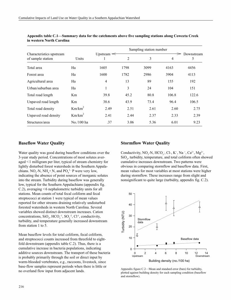
216
Stormflow Water Quality
Conductivity, NO3-N, HCO
3
-, Cl-, K+, Na +, Ca2+, Mg2+,
SiO2, turbidity, temperature, and total coliform often showed
cumulative increases downstream. Two patterns were
obvious in comparing stormflow and baseflow data. First,
mean values for most variables at most stations were higher
during stormflow. These increases range from slight and
nonsignificant to quite large (turbidity, appendix fig. C.2).
Baseflow Water Quality
Water quality was good during baseflow conditions over the
3-year study period. Concentrations of most solutes aver-
aged < 1 milligram per liter, typical of stream chemistry for
lightly disturbed forest watersheds in the Southern Appala-
chians. NO3-N, NH
4+
-N, and PO
4
3—P were very low,
indicating the absence of point sources of inorganic solutes
into the stream. Turbidity during baseflow was generally
low, typical for the Southern Appalachians (appendix fig.
C.2), averaging < 6 nephalometric turbidity units for all
stations. Mean counts of total fecal coliform and fecal
streptococci at station 1 were typical of mean values
reported for other streams draining relatively undisturbed
forested watersheds in western North Carolina. Several
variables showed distinct downstream increases. Cation
concentrations, SiO2, HCO
3
-1, SO4
-2, Cl-1, conductivity,
turbidity, and temperature generally increased downstream
from station 1 to 5.
Mean baseflow levels for total coliform, fecal coliform,
and streptococci counts increased from threefold to eight-
fold downstream (appendix table C.2). Thus, there is a
cumulative increase in bacteria populations, indicating
additive sources downstream. The transport of these bacteria
is probably primarily through the soil or direct input by
warm-blooded vertebrates, e.g., raccoons, livestock, since
base-flow samples represent periods when there is little or
no overland flow input from adjacent lands.Appendix figure C.2—Mean and standard error (bars) for turbidity,
plotted against building density for each sampling condition (baseflow
and stormflow).
Cumulative Impacts of Land Use on Water Quality in a Southern Appalachian Watershed
Appendix table C.1—Summary data for the catchments above five sampling stations along Coweeta Creek
in western North Carolina
Sampling station number
Characteristics upstream Upstream Downstream
of sample station Units 1 2 3 4 5
Total area Ha 1605 1798 3099 4163 4456
Forest area Ha 1600 1782 2986 3904 4113
Agricultural area Ha 4 13 89 155 192
Urban/suburban area Ha 1 3 24 104 151
Total road length Km 39.8 45.2 80.8 106.8 122.6
Unpaved road length Km 38.6 43.9 73.4 96.4 106.5
Total road density Km/km2
2.49 2.51 2.61 2.60 2.75
Unpaved road density Km/km2
2.41 2.44 2.37 2.33 2.39
Structures/area No./100 ha .37 3.06 5.36 6.01 9.23
Building density (no./100 ha)
Turb
idity (
NT
U)
Baseflow data
Stormflowdata
Upstream Downstream0 2 4 6 8 10 12 14
50
40
30
20
10
0

217
Bacteria levels were among the most responsive water-
quality variables during storm events, although patterns
were highly variable among storms and among seasons.
Total coliform, fecal coliform, and fecal streptococci
typically increased twofold to threefold during storm events
compared to baseflow populations. The source of these large
downstream increases in bacteria may be attributed to
observed overland flow from adjacent lands directly into
streams, disturbance of bottom sediments, and streambank
flushing (appendix table C.3, appendix fig. C.3).
Conclusions
In summary, this work identifies consistent, cumulative
downstream changes in Coweeta Creek concomitant with
downstream changes in land use. Furthermore, this work
indicates consistently higher downstream changes during
stormflow when compared to baseflow conditions, suggest-
ing cumulative impacts due to landscape alteration, as tested
here, are much greater during stormflow events.
Literature Cited
Bolstad, P.V.; Swank, W.T. 1997. Cumulative impacts of landuse on water
quality in a Southern Appalachian watershed. Journal of the American
Water Resources Association: 519–533. Vol. 33, no. 3.
Appendix C
Appendix figure C.3—Mean and standard error (bars)
for (A) total coliform and (B) fecal streptococcus, plotted
against building density for each sampling condition
(baseflow and stormflow). (Building density increases
downstream).
Appendix table C.2—Summary water-quality data from
baseflow grab samples (means) at each of the five sampling
stations along Coweeta Creek in western North Carolina
Station number
Variable 1 2 3 4 5
- - - - - - - - - - - Per 100 milliliters - - - - - - - - - - -
Total coliform 9,470 13,660 40,040 30,740 52,140
Fecal coliform 200 340 460 1,130 840
Fecal streptococcus 710 1,310 2,180 1,590 1,840
Appendix table C.3—Summary water-quality data
from stormflow samples (means) at each of the five
sampling stations along Coweeta Creek in western
North Carolina
Station number
Variable 1 2 3 4 5
- - - - - - - - - - Per 100 milliliters - - - - - - - - - -
Total coliform 18,790 34,640 NA 77,160 98,390
Fecal coliform 880 130 NA 970 1,260
Fecal streptococcus 450 8,710 NA 3,260 4,190
NA = Not available.
Building density (no./100 ha)
1000 c
olo
nie
s/1
00 m
L
0 2 4 6 8 10 12 14
160
140
120
100
80
60
40
20
0
Total coliform by building density
Baseflow
Stormflow
(A)
Building density (no./100 ha)
Co
lon
ies/1
00
mL
0 2 4 6 8 10 12 14
7000
6000
5000
4000
3000
2000
1000
0
Fecal streptococcus by building density
Baseflow
Stormflow
(B)

218
Appendix D
Protozoan Pathogens Giardia and Cryptosporidium
David Stern1
Introduction
Two pathogens carried by wildlife, Giardia spp. andCryptosporidium spp., are of great interest in drinking water.Giardia cysts and Cryptosporidium oocysts are parasiticprotozoans. They are active and reproduce within their hostsand encyst to survive in the environment during transmis-sion between hosts. Many species of wildlife have beenfound to be hosts for these parasites (appendix table D.1).These organisms are significant sources of gastrointestinalillness (Jokipii and others 1983, Kenney 1994, Moore andothers 1994). The risk posed by these parasites is believed tobe significant. As little as one cyst may be able to causeinfection (Medema and others 1995, Rose and Gerba 1991,Rose and others 1991). What is more, these organisms areresistant to disinfection (Campbell and others 1982, Clarkand Regli 1993, Craun 1981, Haas and Heller 1990, Hoffand Rubin 1987, Jarroll and others 1981, Kong and others1988, Quinn and Betts 1993, Rice 1981, Rubin and others1989). Although there are medications that are effective intreating giardiasis, currently there are no drugs available totreat infections caused by Cryptosporidium.
Federal Regulation
In 1986, the U.S. Congress recognized the threat posed bythese protozoan parasites and revised the Safe DrinkingWater Act to begin to address this concern. The SurfaceWater Treatment Rule for the Safe Drinking Water Act(SDWA), promulgated in 1991 (U.S. EnvironmentalProtection Agency 1996), requires all surface water suppliesto be filtered prior to distribution to the public, unless it canbe demonstrated that a certain level of purity exists and canbe maintained. The Surface Water Treatment Rule empha-sizes water supply filtration because disinfecting by chlori-nation does not eliminate the threat posed by Giardia andCryptosporidium (Campbell and others 1982, Clark andothers 1989). Accordingly, prevention or filtration isrecommended as the response to this threat. In its continu-ance of concern for the threat posed by Giardia andCryptosporidium, the Federal Government enacted 1996amendments to the SDWA to fund additional watershedresearch on these organisms.
Giardia
To survive in the environment, Giardia encysts itself into aresistant form. Giardia cysts are 5 to 15 microns in size andoblong in shape. Early research on this parasitic protozoanidentified it on the basis of median body morphology andthe host it was found in. Accordingly, Giardia species are G.muris, G. agilis, and G. duodenalis and are usually found inrodents, frogs, and warm-blooded vertebrates, respectively.This early nomenclature was due to the assumption thatGiardia was highly host-specific. More recent research hasshown that Giardia can cross-infect different species ofhosts (Meyer and Jarroll 1980).
Identification of Giardia as a waterborne parasite forhumans was first reported in the 1940’s during a study of adisease outbreak in an apartment building in Tokyo, Japan(Davis 1948). Giardia has more recently been reported asthe most frequently identified parasite responsible fordisease outbreaks in surface water supplies in NorthAmerica (Craun 1984). A significant portion of the literaturehas reported on the occurrence, disinfection, and treatmentof Giardia cysts.
The life cycle for Giardia has been described by Meyer andJarroll (1980). Giardia is monoxenous, which means that allof its life stages occur in one host. These stages include aninactive cyst form that is capable of resisting environmentalstresses and a free-living form known as a trophozoite. Thetrophozoite has a ventral sucker disk that attaches to theintestinal wall to obtain subsidence. The life cycle consistsof: (1) a host ingesting the cyst, (2) excystation (emergenceof the trophozoite out of the cyst) occurring in the smallintestine after the cyst has been subjected to the digestiveenvironment, (3) the released trophozoite attaching to theintestinal wall where it feeds and reproduces by binaryfission, and (4) some of the reproduced trophozoites encystwithin the intestine and the resultant cyst is excreted in theinfected animal’s feces to be transmitted to other hosts.
Cryptosporidium
Cryptosporidium was first identified by Tyzzer (1910) over
90 years ago as a parasite of the common mouse. Its1 Pathogen Program Supervisor, New York City, Department of Environ-mental Protection, Valhalla, NY.

219
Appendix table D.1—Species reported as hosts to protozoans Giardia and Cryptosporidium
Species Common name Parasites hosted
Pisces
Cyprinus carpio Carp Cryptosporidium
Sciaenops ocellatus Red drum Cryptosporidium
Plecostomus spp. Catfish Cryptosporidium
Salmo trutta Brown trout Cryptosporidium
Oncorhynchus mykiss Rainbow trout Cryptosporidium
Amphibia
Ceratophrys ornata Bell’s horned frog Cryptosporidium
Bufo americanus American toad Cryptosporidium
B. regularis Common toad Giardia
Rana pipiens Leopard frog Giardia
R. clamitans Green frog Giardia
Reptilia
Chelonia mydas Green turtle Cryptosporidium
Geochelone elegans Star tortoise Cryptosporidium
G. carbonaria Red-footed tortoise Cryptosporidium
Squamata Lacertilia (lizards)
Agama aculeata Kalahari spiny agama Cryptosporidium
A. planiceps Damara rock agama Cryptosporidium
Chameleo c. senegalensis Chamelon Cryptosporidium
Chamaeleo pardalis Panther chamelon Cryptosporidium
Chlamydosaurus kingi Frilled lizard Cryptosporidium
Lacerta lepida Ocellated lacerta Cryptosporidium
Chondrodactylus angulifer Sand gecko Cryptosporidium
Serpentes (snakes)
Crotalus durissus culminatus Rattlesnake Cryptosporidium
Sistrurus miliarius Pygmy rattlesnake Cryptosporidium
Lampropeltis getulus holbrooki Say’s kingsnake Giardia
Elaphe subocularis Trans-Pecos rat snake Cryptosporidium
E. o. obsoleta Black rat snake Cryptosporidium
E. o. quadrivittata Yellow rat snake Cryptosporidium
E. o. lindheimeri Texas rat snake Cryptosporidium
E. guttata Corn snake Cryptosporidium
E. v. vulpina Western fox snake Cryptosporidium
Gonysoma oxycephala Red-tailed green rat snake Cryptosporidium
Pituophis melanoleucus Black pine snake Cryptosporidium
P. melanoleucus catenifer Gopher snake Cryptosporidium
Drymarchon corais couperi Eastern indigo snake Cryptosporidium
Lampropeltis zonata pulchura San Diego mountain snake Cryptosporidium
L. triangulum Various subspecies Cryptosporidium
Nerodia h. harteri Brazos water snake Cryptosporidium
N. r. rhombifera Diamondback water snake Cryptosporidium
Boiga dendrophila Mangrove snake Cryptosporidium
C. horridus Timber rattlesnake Cryptosporidium
C. atrioca udatus Canebrake rattlesnake Cryptosporidium
C. l. lepidus Rock rattlesnake Cryptosporidium
continued
Appendix D

220
Protozoan Pathogens Giardia and Cryptosporidium
Appendix table D.1—Species reported as hosts to protozoans Giardia and Cryptosporidium (continued)
Species Common name Parasites hosted
Aves
Anseriformes
Branta canadensis Canada goose Cryptosporidium, Giardia
Anser anser Domestic goose Cryptosporidium
Cygnus spp. Tundra swan Cryptosporidium
C. olor Mute swan Cryptosporidium
Aix sponsa Wood duck Cryptosporidium
Anas platyrrhynchos Mallard duck Cryptosporidium
Mergus merganser Common merganser Cryptosporidium
Columbiformes
Columba livia Pigeon Cryptosporidium
Galliformes
Gallus gallus Chicken Cryptosporidium
Meleagris gallopavo Turkey Cryptosporidium
Coturnix coturnix Common quail Cryptosporidium
Colinus virginianus Bobwhite quail Cryptosporidium
Phasianus colchicus Ring-necked pheasant Cryptosporidium
Pavo cristatus Peafowl Cryptosporidium
Perdix perdix Grey partridge Cryptosporidium
Alectoris graeca Chuckar partridge Cryptosporidium
Numida meleagris Guinea fowl Cryptosporidium
Charadriiformes
Larus ridibundus Black-headed gull Cryptosporidium
L. argentatus Herring gull Cryptosporidium
L. delawarensis Ring-billed gull Cryptosporidium
Recurvirostra avosetta Avocet Giardia
Threskiornis spinicollis Straw-necked ibis Giardia
Passeriformes
Poephila cincta Black-throated finch Cryptosporidium
Lonchura cucullata Bronze mannikin finch, Cryptosporidium
red cheek finch
Passer domesticus House sparrow Giardia
Zonotrichia georgiana Swamp sparrow Giardia
Sturnella neglecta Western meadowlark Giardia
Lanius collurio Red-backed shrike Giardia
Ciconiiformes
Ardea herodias Great blue heron Giardia
A. cinerea Gray heron Giardia
A. cocoi Cocoi heron Giardia
Egretta alba Great egret Giardia
E. caerulea Little blue heron Giardia
Nycticorax nyctocorax Black-crowned night-heron Giardia
N. naevius Night-heron Giardia
Butorides virescens Green-backed heron Giardia
Egretta intermedia Intermediate egret Giardia
Bubulcus ibis Cattle egret Giardia
Botaurus lentiginosus American bittern Giardia
Ixobrychus minutus Little bittern Giardia
Plegadis falcinellus Glossy ibis Giardia
continued

221
Appendix table D.1—Species reported as hosts to protozoans Giardia and Cryptosporidium (continued)
Species Common name Parasites hosted
Aves (continued)
Falconiformes
Cathartes aura Turkey vulture Giardia
Elanus caeruleus Black-winged kite Giardia
Mammalia
Marsupialia
Didelphis virginiana Virginia opossum Cryptosporidium, Giardia
Pseudocheirus peregrinus Possum Giardia
Insectivora
Sorex spp. Shrew Giardia
Blarina brevicauda Short-tailed shrew Cryptosporidium, Giardia
S. cinereus Masked shrew Cryptosporidium
Parascalops breweri Hairy-tailed mole Cryptosporidium
Myotis lucifugus Little brown bat Cryptosporidium
Eptesicus fuscus Big brown bat Cryptosporidium, Giardia
Lagomorpha
Sylvilagus floridanus Eastern cottontail Cryptosporidium, Giardia
Rodentia
Ondatra zibethica Common muskrat Cryptosporidium, Giardia
Microtus agrestis Field vole Cryptosporidium
M. chrotorrhinus Rock vole Giardia
M. pennsylvanicus Meadow vole Cryptosporidium, Giardia
M. pinetorum Pine vole Giardia
M. longicaudus Long-tailed vole Giardia
M. ochrogaster Prairie vole Giardia
M. californicus Meadow vole Giardia
M. richardsoni Water vole Giardia
Clethrionomys glareolus Bank vole Cryptosporidium
C. glareolus skomerensis Skomer bank vole Cryptosporidium
Apodemus sylvaticus Wood mouse Cryptosporidium
Rattus rattus Roof rat or ship rat Cryptosporidium, Giardia
Sigmodon hispidus Cotton rat Cryptosporidium
Erithizon dorsatum Porcupine Cryptosporidium, Giardia
Mus musculus House mouse Cryptosporidium, Giardia
Zapus hudsonicus Meadow jumping mouse Giardia
Napaeozapus insignis Woodland jumping mouse Giardia
Peromyscus leucopus White-footed mouse Cryptosporidium, Giardia
P. maniculatus Deer mouse Cryptosporidium, Giardia
C. gapperi Red-backed vole Cryptosporidium, Giardia
Pitymys savii Savi’s woodland vole Giardia
R. norvegicus Norway rat Cryptosporidium, Giardia
Neotoma cinerea Wood rat Giardia
Dipodomys heermanni Kangaroo rat Giardia
Tamia striatus Eastern chipmunk Cryptosporidium, Giardia
Sciurus carolinensis Eastern gray squirrel Cryptosporidium, Giardia
Tamiasciurus hudsonicus Red squirrel Cryptosporidium, Giardia
Glaucomys volans Southern flying squirrel Giardia
continued
Appendix D

222
Protozoan Pathogens Giardia and Cryptosporidium
Appendix table D.1—Species reported as hosts to protozoans Giardia and Cryptosporidium (continued)
Species Common name Parasites hosted
Mammelia (continued)
Rodentia (continued)
Spermophilus beecheyi Ground squirrel Giardia
S. richardsoni Richardson’s ground squirrel Giardia
S. tridecemlineatus 13-lined ground squirrel Giardia
Marmota monax Woodchuck Cryptosporidium, Giardia
Coendu villosus Tree porcupine Giardia
Carnivora
Ursus americanus Black bear Cryptosporidium
Mustela erminea Short-tailed weasel Cryptosporidium
M. putorius furo Ferret Cryptosporidium
Canis latrans Coyote Cryptosporidium, Giardia
Vulpes vulpes Red fox Giardia
Urocyon cineroargenteus Gray fox Cryptosporidium, Giardia
Procyon lotor Raccoon Cryptosporidium, Giardia
Paradoxurus h. hermaphroditus Palm civet Giardia
Mephitis mephitis Striped skunk Cryptosporidium, Giardia
Mustela vision Mink Cryptosporidium, Giardia
M. nigripes Black-footed ferret Giardia
Meles meles Badger Giardia
Lynx rufus Bobcat Cryptosporidium, Giardia
Sirenia
Dugong dugong Manatee Cryptosporidium
Ruminants
Cervus canadensis Elk, wapiti Giardia
Odocoileus virginiana White-tailed deer Cryptosporidium, Giardia
Antilocapra americana Pronghorn Giardia
Ovis canadensis x. O. musimon Bighorn x mouflon sheep Giardia
Llama glama Llama Cryptosporidium, Giardia
Odocoileus hemionus Mule deer Cryptosporidium
Source: Adapted from Wade and others, in press.
223
significance began to be recognized in the 1970’s when a
number of reports identified Cryptosporidium as the cause
of diarrhea in calves (O’Donoghue 1995). Human infections
began to be reported in the mid-1970’s and by the 1990’s,
Cryptosporidium was recognized as a significant threat to
individuals that are immunocompromised (Current and
Garcia 1991, Ungar 1990).
Cryptosporidium oocysts are spherical and 4 to 6 microns in
diameter (Barer and Wright 1990, Casemore 1991,
Casemore and others 1985, Current 1987, Current and
others 1986, Fayer and Ungar 1986, Issac-Renton and others
1987, O’Donoghue 1995, Smith and Rose 1990, Ungar
1994). Most oocysts contain up to four sporozoites (free-
living form). A number of species have been identified
among various hosts. Many of these species can cross-infect
different species of hosts. Several Cryptosporidium species
are found more often in association with certain host
species, especially when the host species are vertebrates.
Thus, C. muris is common in mammals, C. meleagridis in
birds, C. crotalia in reptiles, and C. nasorum in fish (Levine
1984, O’Donoghue 1995).
O’Donoghue (1995) and Current and Bick (1989) described
the life cycle for Cryptosporidium. Like Giardia,
Cryptosporidium encysts to survive outside its host, and its
life stages occur in the infected animal. Its life cycle is more
complex due to the addition of a sexual stage of reproduc-
tion within the host. The oocyst of Crypto-sporidium
undergoes excystation (release of sporozoites) after it has
been ingested by a host and has been subjected to conditions
usually found in a digestive system. These conditions have
been identified as including temperature, low pH, and
digestive enzymes (Fayer and Leek 1984, Reduker and
Speer 1985). The released sporozoites attach to epithelial
cells of the small intestine, where they are identified as
trophozoites (Cryptosporidium attached to intestine). The
trophozoites mature into meronts that produce merozoites
through asexual reproduction. The merozoites, in turn,
develop into either other meronts or produce the sexual form
of Cryptosporidium, microgametes (male form) and
macrogametes (female form). The mobile microgametes
fertilize the macrogametes in sexual reproduction to form a
zygote (the sexually reproduced form of Cryptosporidium).
Most of the zygotes form thick-walled oocysts that are
released from the host to infect other hosts and complete the
life cycle.
Literature Cited
Barer, R.R.; Wright, A.E. 1990. Cryptosporidium and water. Applied
Microbiology. 11(6): 271–277.
Campbell, I.; Tzipori, S.; Hutcinson, G.; Angus, K.W. 1982. Effects of
disinfection on survival of Cryptosporidium oocysts. Veterinary Record.
111(18): 414–415.
Casemore, D.P. 1991. Epidemiology of human Cryptosporidiosis and the
water route of infection. Water Science and Technology. 24(2): 157–164.
Casemore, D.P.; Sands, R.L.; Curry, A. 1985. Cryptosporidium species a
“ new “ human pathogen. Journal of Clinical Pathology. 38(12):
1321–1336.
Clark, R.M.; Read, E.J.; Hoff, J.C. 1989. Analysis of inactivation of
Giardia lamblia by chlorine. Journal of Environmental Engineering.
115(1): 80–90.
Clark, R.M.; Regli, S. 1993. Development of Giardia Ct values for the
surface water treatment rule. Journal of Environmental Science and
Health. 28(5): 1081–1097.
Craun, G.F. 1981. Disease outbreaks caused by drinking water. Journal of
the Water Pollution Control Federation. 53(6): 1134–1138.
Craun, G.F. 1984. Waterborne outbreaks of giardiasis. Current status. In:
Erlandsen, S.L.; Meyer, E.A., eds. Giardia and giardiasis. New York:
Plenum Press: 243–262.
Current, W.L. 1987. Cryptosporidium: its biology and potential for
environmental transmission. CRC Critical Reviews in Environmental
Control. 17(1): 21–51.
Current, W.L.; Bick, P. 1989. Immunobiology of Cryptosporidium spp.
Pathology and Immunopathology Research. 8: 141–160.
Current, W.L.; Garcia, L.S. 1991. Cryptosporidiosis. Clinical Microbiol-
ogy Reviews. 4: 325–358.
Current, W.L.; Upton, S.J.; Haynes, T.B. 1986. The life cycle of
Cryptosporidium baileyi n.sp. (Apicomplexa, Cryptosporidiidae )
infecting chickens. Journal of Protozoology. 33: 29–296.
Davis, C.; Ritchie, L.S. 1948. Clinical manifestations and treatment of
epidemic amebiasis occurring in occupants of the Mantetsu apartment
building. Tokyo: American Journal of Tropical Medicine. 28: 817–823.
Fayer, R.; Leek, R.G. 1984. The effects of reducing conditions, medium,
pH, temperature, and time on in vitro excystation of Cryptosporidium.
Journal of Protozoa. 31: 567–569.
Fayer, R.; Ungar, B.L.P. 1986. Cryptosporidium spp. and Crypto-
sporidiosis. Microbiol.Reviews. 50(4): 458–483.
Haas, C.N.; Heller, B. 1990. Kinetics of inactivation of Giardia lamblia by
free chlorine. Water Research. 24(4): 233–238.
Hoff, J.C.; Rubin, A.J. 1987. Use of inactivation rate data for establishing
drinking water disinfection requirements for Giardia cyst control. In:
Preprints of papers presented at the 194th American chemical society
national meeting; [Date of meeting unknown]; Washington, DC.
Washington, DC: American Chemical Society, Division of Environmen-
tal Chemistry: 760–763. Vol. 27, no.2.
Appendix D

224
Reduker, D.W.; Speer, C.A. 1985. Factors influencing excystation of
Cryptosporidium oocysts from cattle. Journal of Parasitology. 71(1):
112–115.
Rice, G.R. 1981. Use of ozone in drinking water treatment. Journal
American Water Works Association. 73(1): 44.
Rose, J.B.; Gerba, C.P. 1991. Use of risk assessment for development of
microbial standards. Water Science and Technology. 24(2): 29–34.
Rose, J.B.; Haas, C.N.; Regli, S. 1991. Risk assessment and control of
waterborne Giardiasis. American Journal of Public Health. 81(6):
709–713.
Rubin, A.J.; Evers, D.P.; Eyman, C.M.; Jarroll, E.L. 1989. Inactivation
of gerbil-cultured Giardia lamblia cysts by free chlorine: Applied and
Environmental Microbiology. 55(10): 2592–2594.
Smith, H.V.; Rose, J.B. 1990. Waterborne Cryptosporidiosis. Parasitology
Today. 6(1): 8–12.
Tyzzer, E.E. 1910. An extracellular coccidium, Cryptosporidium muris, of
the gastric glands of the common mouse. Journal of Medical Research.
23: 487–509.
Ungar, B.L.P. 1990. Cryptosporidiosis in humans (Homo sapiens). Boston:
CRC Press: 59–82.
Ungar, B.L.P. 1994. Cryptosporidium and Cryptosporidiosis. Textbook of
aids medicine. Baltimore: Williams and Wilkins: 323–343.
Wade, S.E.; Ziegler, P.E.; Schaff, S.L. [In press]. Preliminary investiga-
tion of Giardia species and Cryptosporidium species in wildlife in the
New York City watershed. Final report. Ithaca, NY: Cornell University,
College of Veterinary Medicine, Department of Population Medicine and
Diagnostic Science.
Issac-Renton, J.L.; Fogel, D.; Stibbs, H.H.; Ongerth, J.E. 1987. Giardia
and Cryptosporidium in drinking water. The Lancet. April: 973–974.
Jarroll, E.L.; Bingham, A.K.; Meyer, E.A. 1981. Effect of chlorine on
Giardia lamblia cyst viability. Applied and Environmental Microbiol-
ogy. 41(2): 483–487.
Jokipii, L.; Pohjola, S.; Jokipii, A.M.M. 1983. Cryptosporidium: a
frequent finding in patients with gastrointestinal symptoms. The Lancet.
2(8346): 358–842.
Kenney, R.T. 1994. Parasitic causes of diarrhea. Pediatric Annals. 23(8):
414–421.
Kong, L.I.; Swango, L.J.; Blagburn, B.L. [and others]. 1988. Inactiva-
tion of Giardia lamblia and Giardia canis cysts by combined and free
chlorine. Applied and Environmental Microbiology. 54(10): 2580–2582.
Levine, N.D. 1984. Taxonology and review of the Cooidian Genus
Cyrptosporidium (Protozoa, Aploomiexa). Journal of Protozoology. 31:
94–98.
Medema, G.J.; Van Asperen, I.A.; Klokman Houweling, J.M. [and
others]. 1995. The relationship between health effects in triathletes and
microbiological quality of freshwater. Water-Science-Technology.
31(5–6): 19–26.
Meyer, E.A.; Jarroll, E.L. 1980. Giardia and giardiasis. American Journal
of Epidemiology. 111: 1–12.
Moore, A.C.; Herwaldt, B.L.; Craun, G.F. [and others]. 1994.
Waterborne disease in the United States, 1991 and 1992. Journal
American Water Works Association. February: 87–99.
O’Donoghue, P.J. 1995. Cryptosporidium and Cryptosporidiosis in man
and animals. International Journal for Parasitology. 25(2): 139–195.
Quinn, C.M.; Betts, W.B. 1993. Longer term viability status of chlorine-
treated Crypyosporidium oocysts in tap water. Biomedical Letter. 48:
315–318.
Protozoan Pathogens Giardia and Cryptosporidium

225
Appendix E
Water Treatment Technologies Tables
Gary Logsdon1
Most raw water is not suitable for human consumption
without treatment. Some water only needs to be filtered and
disinfected before consumption (Committee on Small Water
Supply Systems, National Research Council 1997). Other
water must be treated with additional processes to remove
specific chemical contaminants or nuisance chemicals like
iron and manganese. Appendix tables E.1 to E.4 present
information on water treatment techniques that can be used
for controlling common contaminants. The tables provide
guidance on selecting the appropriate treatment processes.
However, a water treatment specialist must select the best
process on a site-specific basis. Additional information can
be found in recent volumes of Water Quality and Treatment
(Letterman 1999) and Safe Water from Every Tap (Commit-
tee on Small Water Supply Systems, National Research
Council 1997).
1 Director, Black and Veatch, Water Process Research, Cincinnati, OH.
Literature Cited
Committee on Small Water Supply Systems, National Research
Council. 1997. Safe water from every tap: improving water service to
small communities. Washington, DC: National Academy Press. 230 p.
Letterman, R.D., tech. ed. 1999. Water quality and treatment. 5th ed.
New York: McGraw-Hill, Inc. 1,248 p.

226
Water Treatment Technologies Tables
Appendix table E.1—Water treatment technologies by disinfectants, oxidants, and aerationa
General water Free Chlorine Potassium Ultraviolet
quality-constituent chlorine Chloramine dioxide Ozone permanganate radiation Aeration
General water qualities
Turbidity, sediment
Color x x x x
Disinfection by-product
precursors
Taste and odor x x x x x
Biological contaminants
Algae
Protozoa x x x x
Bacteria x x x x x
Viruses x x x x x
Organic chemicals
Volatile organics x
Semi-volatile compounds
Pesticides and herbicides
Biodegradable organic
matter
Inorganic chemicals
Hardness
Ironb
x x x x x
Manganeseb
x x x x
Arsenic
Selenium
Thallium
Fluoride
Radon x
Radium
Uranium
Cations
Anions
Total dissolved solids
Nitrate
Ammonia
a The columns and rows lacking x’s are where process is not appropriate or recommended for the constituent.
b When oxidant is followed by filtration.
Source: Table adapted from Committee on Small Water Supply Systems, National Research Council 1997.

227
Appendix table E.2—Water treatment technologies by type of adsorption and ion exchange systema
General water Powdered Granulated Ion Activated
quality-constituent activated carbon activated carbon exchange alumina
General water qualities
Turbidity, sediment
Color x x
Disinfection by-product
precursors x x
Taste and odor x x
Biological contaminants
Algae x
Protozoa x
Bacteria x
Viruses x
Organic chemicals
Volatile organics x x
Semi-volatile compounds x x
Pesticides and herbicides x x
Biodegradable organic
matter x x
Inorganic chemicals
Hardness x
Iron
Manganese
Arsenic x
Selenium x
Thallium x
Fluoride x x
Radon
Radium x
Uranium x
Cations x
Anions x
Total dissolved solids
Nitrate x
Ammonia
a The columns and rows lacking x’s are where process is not appropriate or recommended for the constituent.
Source: Table adapted from Committee on Small Water Supply Systems, National Research Council 1997.
Appendix E
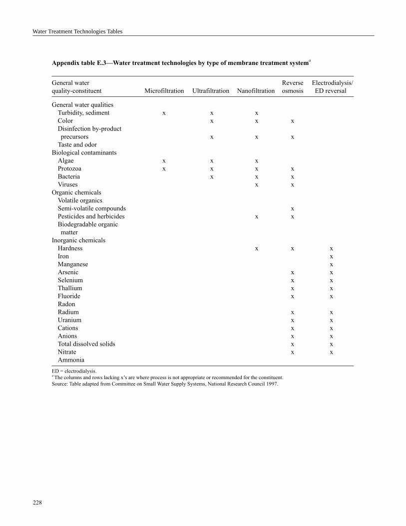
228
Water Treatment Technologies Tables
Appendix table E.3—Water treatment technologies by type of membrane treatment systema
General water Reverse Electrodialysis/
quality-constituent Microfiltration Ultrafiltration Nanofiltration osmosis ED reversal
General water qualities
Turbidity, sediment x x x
Color x x x
Disinfection by-product
precursors x x x
Taste and odor
Biological contaminants
Algae x x x
Protozoa x x x x
Bacteria x x x
Viruses x x
Organic chemicals
Volatile organics
Semi-volatile compounds x
Pesticides and herbicides x x
Biodegradable organic
matter
Inorganic chemicals
Hardness x x x
Iron x
Manganese x
Arsenic x x
Selenium x x
Thallium x x
Fluoride x x
Radon
Radium x x
Uranium x x
Cations x x
Anions x x
Total dissolved solids x x
Nitrate x x
Ammonia
ED = electrodialysis.a The columns and rows lacking x’s are where process is not appropriate or recommended for the constituent.
Source: Table adapted from Committee on Small Water Supply Systems, National Research Council 1997.

229
Appendix table E.4—Water treatment technologies by type of filtration systema
General water Direct Conventional Dissolved Precoat Slow sand Bag/cartridge Lime
quality-constituent filtration filtration air flotation filtration filtration filters softening
General water qualities
Turbidity, sediment x x x x x x
Color x x x
Disinfection by-product
precursors x x x
Taste and odor x
Biological contaminants
Algae x x x
Protozoa x x x x x x x
Bacteria x x x x x x
Viruses x x x x x x
Organic chemicals
Volatile organics
Semi-volatile compounds
Pesticides and herbicides
Biodegradable organic
matter x* x* x* x
Inorganic chemicals
Hardness x
Iron x x x x x
Manganese x x x x x
Arsenic x x x
Selenium x
Thallium
Fluoride
Radon
Radium x
Uranium
Cations x
Anions
Total dissolved solids
Nitrate
Ammonia x* x* x* x
X* = when the filter is operated in a biologically active mode.a The columns and rows lacking x’s are where process is not appropriate or recommended for the constituent.
Source: Table adapted from National Research Council 1997.
Appendix E
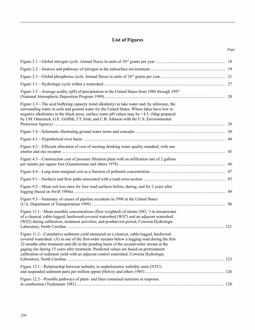
230
List of Figures
Page
Figure 2.1—Global nitrogen cycle. Annual fluxes in units of 1012 grams per year .................................................................. 18
Figure 2.2—Sources and pathways of nitrogen in the subsurface environment ....................................................................... 19
Figure 2.3—Global phosphorus cycle. Annual fluxes in units of 1012 grams per year ............................................................. 21
Figure 3.1—Hydrologic cycle within a watershed .................................................................................................................... 27
Figure 3.2—Average acidity (pH) of precipitation in the United States from 1988 through 1997
(National Atmospheric Deposition Program 1999) ................................................................................................................... 28
Figure 3.3—The acid buffering capacity (total alkalinity) in lake water and, by inference, the
surrounding water in soils and ground water for the United States. Where lakes have low or
negative alkalinities in the black areas, surface water pH values may be < 4.5. (Map prepared
by J.M. Omernick, G.E. Griffith, J.T. Irish, and C.B. Johnson with the U.S. Environmental
Protection Agency) .................................................................................................................................................................... 29
Figure 3.4—Schematic illustrating ground water terms and concepts ...................................................................................... 30
Figure 4.1—Hypothetical river basin ........................................................................................................................................ 44
Figure 4.2—Efficient allocation of cost of meeting drinking water quality standard, with one
emitter and one receptor ............................................................................................................................................................ 45
Figure 4.3—Construction cost of pressure filtration plant with an infiltration rate of 2 gallons
per minute per square foot (Gummerman and others 1978) ...................................................................................................... 46
Figure 4.4—Long-term marginal cost as a function of pollutant concentration ....................................................................... 47
Figure 9.1—Surfaces and flow paths associated with a road cross section .............................................................................. 85
Figure 9.2—Mean soil loss rates for four road surfaces before, during, and for 2 years after
logging (based on Swift 1984a) ................................................................................................................................................. 89
Figure 9.3—Summary of causes of pipeline accidents in 1998 in the United States
(U.S. Department of Transportation 1999) ................................................................................................................................ 96
Figure 11.1—Mean monthly concentrations (flow weighted) of nitrate (NO3
-1) in streamwater
of a clearcut, cable-logged, hardwood-covered watershed (WS7) and an adjacent watershed
(WS2) during calibration, treatment activities, and postharvest period, Coweeta Hydrologic
Laboratory, North Carolina ....................................................................................................................................................... 121
Figure 11.2—Cumulative sediment yield measured on a clearcut, cable-logged, hardwood-
covered watershed: (A) in one of the first-order streams below a logging road during the first
32 months after treatment and (B) in the ponding basin of the second-order stream at the
gaging site during 15 years after treatment. Predicted values are based on pretreatment
calibration of sediment yield with an adjacent control watershed, Coweeta Hydrologic
Laboratory, North Carolina ....................................................................................................................................................... 123
Figure 12.1—Relationship between turbidity in nephelometric turbidity units (NTU)
and suspended sediment parts per million (ppm) (Helvey and others 1985) ............................................................................ 126
Figure 12.2—Possible pathways of plant- and litter-contained nutrients in response
to combustion (Tiedemann 1981) .............................................................................................................................................. 128

231
Page
Figure 14.1—Potential sediment production in 10 Blue Mountain ecosystems in Oregon.
Ecosystems: L = larch, M = meadow, LP = lodgepole pine, DF = Douglas fir, A = alpine,
PP = ponderosa pine, SF = spruce-fir, G = grassland, SA = sagebrush, J = juniper
(Buckhouse and Gaither 1982). Different lower-case letters indicate differences in statistical
significance (P < 0.10) ................................................................................................................................................................ 154
Appendix figure A.1—Watersheds supplying Baltimore, MD, with water ............................................................................... 210
Appendix figure B.1—Location of Quabbin Reservoir and water supply system
for Boston, MA .......................................................................................................................................................................... 213
Appendix figure C.1—Watershed boundary and stream sampling locations in the Coweeta
Creek Watershed in western North Carolina. Stations 1 through 5 are arranged down the
stream gradient on Coweeta Creek. First-order streams are not shown .................................................................................... 215
Appendix figure C.2—Mean and standard error (bars) for turbidity, plotted against building
density for each sampling condition (baseflow and stormflow) ............................................................................................... 216
Appendix figure C.3—Mean and standard error (bars) for (A) total coliform and (B) fecal
streptococcus, plotted against building density for each sampling condition (baseflow and
stormflow). (Building density increases downstream) .............................................................................................................. 217
List of Figures

232
List of Tables
Page
Table 2.1—Summary of common water pollutants by land-use activities ............................................................................... 8
Table 2.2—Common types of water contaminant guidelines for different water uses ............................................................. 8
Table 2.3—National primary drinking water regulations (States are expected to focus attention
on risks related to the contaminants listed in their source water assessments.) ........................................................................ 9
Table 2.4—National secondary drinking water regulations, which are nonenforceable guidelines
for contaminants that may cause cosmetic effects (e.g., skin or tooth discoloration) or aesthetic
effects (e.g., taste, odor, or color) in drinking water ................................................................................................................. 14
Table 2.5—Common chemical processes involved as water interacts with its environment ................................................... 15
Table 2.6—Summary of the chemical behavior of important water contaminants ................................................................... 16
Table 2.7—Common waterborne pathogenic and indicator bacteria and viruses ..................................................................... 23
Table 2.8—Factors influencing virus transport and fate in the subsurface ............................................................................... 24
Table 6.1—Reported acres inside national forest boundaries and percent population changes in
counties containing or adjacent to national forests by administrative Forest Service Region in the
conterminous United States ....................................................................................................................................................... 63
Table 6.2—Estimated use from freshwater surface and ground water sources in the
United States, 1980–95 ............................................................................................................................................................. 64
Table 6.3—Waterborne disease outbreaks in the United States by water supply system, 1990–94 ......................................... 64
Table 6.4—Comparison of outbreak percentages by drinking water source from pathogenic
contamination for the period 1971–96 ...................................................................................................................................... 64
Table 9.1—Typical erosion rates observed for different types of land use in the United States .............................................. 88
Table 9.2—Effectiveness of erosion mitigation techniques ...................................................................................................... 89
Table 9.3—Management options for decommissioned roads ................................................................................................... 91
Table 9.4—Pollutants that have been observed in runoff from road surfaces .......................................................................... 93
Table 9.5—Mean concentrations of a number of pollutants in highway runoff in Minnesota ................................................. 93
Table 9.6—Extent of soil contamination by 53 oil spills of various sizes in Alberta, Canada ................................................. 96
Table 10.1—Effects of various timber harvests or site preparations on soil erosion and
sediment production .................................................................................................................................................................. 105
Table 10.2—Effects of timber harvesting with and without streamside buffers
on stream temperature ............................................................................................................................................................... 109
Table 10.3—Effects of clearcutting with and without buffers on mean annual nitrate-nitrogen,
ammonium-nitrogen, and total-phosphorus concentrations ...................................................................................................... 112
Table 10.4—Effects of forest fertilization on maximum streamwater ammonium-nitrogen and
nitrate-nitrogen concentrations .................................................................................................................................................. 114
Table 12.1—Water turbidity, in Jackson turbidity units (equivalent to nephelometric turbidity
units), after fire alone or in combination with other treatments ................................................................................................ 125
Table 12.2—Suspended sediment concentration in streamflow after fire alone or in
combination with other treatments ............................................................................................................................................ 125

233
Page
Table 12.3—Sediment yield after fire alone or in combination with other treatments ............................................................. 127
Table 12.4—The pH in water after fire alone or in combination with other treatments ........................................................... 130
Table 12.5—Maximum nitrate-nitrogen concentration in water after fire alone or in
combination with other treatments ............................................................................................................................................ 131
Table 12.6—Sulfate concentration in water after fire alone ..................................................................................................... 133
Table 12.7—Chloride concentration in water after fire alone ................................................................................................... 133
Table 13.1—Management uses of pesticides commonly used on national forests ................................................................... 141
Table 13.2—Estimates of safe levels for daily exposure to the 20 pesticides most used
on National Forest System lands in fiscal year 1997 in the vegetation management program ................................................ 142
Table 13.3—Frequency and occurrence of surface and ground water contamination
from pesticide use in North America ........................................................................................................................................ 144
Table 15.1—Streamwater fecal coliform and Giardia responses to herbivore use................................................................... 161
Table 16.1—Indicator and principal pathogens of concern in contaminated drinking water ................................................... 165
Appendix table C.1—Summary data for the catchments above five sampling stations
along Coweeta Creek in western North Carolina ...................................................................................................................... 216
Appendix table C.2—Summary water-quality data from baseflow grab samples (means) at
each of the five sampling stations along Coweeta Creek in western North Carolina ............................................................... 217
Appendix table C.3—Summary water-quality data from stormflow samples (means) at each
of the five sampling stations along Coweeta Creek in western North Carolina ....................................................................... 217
Appendix table D.1—Species reported as hosts to protozoans Giardia and Cryptosporidium ................................................ 219
Appendix table E.1—Water treatment technologies by disinfectants, oxidants, and aeration .................................................. 226
Appendix table E.2—Water treatment technologies by type of adsorption and
ion exchange system ................................................................................................................................................................. 227
Appendix table E.3—Water treatment technologies by type of membrane treatment system .................................................. 228
Appendix table E.4—Water treatment technologies by type of filtration system ..................................................................... 229
List of Tables

234
Glossary of Abbreviations and Acronyms
ai: active ingredient
aum: animal unit month
BAER: Burn Area Emergency Rehabilitation
BLM: Bureau of Land Management
BMP: best management practice
BOD: biological oxygen demand
Bt: Bacillus thuringiensis
BTEX: benzene, toluene, ethylbenzene, xylene
C: carbon
Ca: calcium
Ca2+: calcium ion
Ca(HCO3)
2: calcium bicarbonate
Cd: cadmium
CDC: Centers for Disease Control and Prevention
CERLA: Comprehensive Environmental Response,
Compensation and Liability Act
CH4: methane
Cl: chlorine
Cl-1: chloride ion
cm: centimeter
CO2: carbon dioxide
COD: chemical oxygen demand
Cu: copper
CWD: coarse woody debris
DEP: City of New York Department of Environmental
Protection
DO: dissolved oxygen
DOD: Department of Defense
EPA: U.S. Environmental Protection Agency
ET: evapotranspiration
F: fluorine
FC: fecal coliform
FDA: U.S. Food and Drug Administration
Fe+2: ferrous iron ion
Fe+3: ferric iron ion
Fe3S
4:
greigite
FeS: pyrite
FeS2: marcasite
FIFRA: Federal Insecticide, Fungicide,
and Rodenticide Act
FS: fecal streptococcus
GIS: Geographic Information System
H+: hydrogen ion
H2S: hydrogen sulfide
ha: hectare
HA or HAL: health advisory level
HCN: hydrogen cyanide
HCO3
-1: bicarbonate ion
HTH: chlorine
JTU: Jackson turbidity unit
K: potassium

235
K+: potassium ion
km: kilometer
LOAEL: lowest observed adverse effect level
m: meter
MCL: maximum contaminant level
MCLG: maximum contaminant level goal
MD-DNR: Maryland Department of Natural Resources
MDC-DWM: Metropolitan District Commission’s
Division of Watershed Management (Massachusetts)
Mg: magnesium
Mg2+: magnesium ion
mg: milligram
Mg: metric tonne or megagram
µg: microgram
µm: micron or 1 millionth of a meter
Mg(HCO3)
2: magnesium bicarbonate
MgSO4: magnesium sulfate
MITC: methyl isothiocyanate
Mn: manganese
MTBE: methyl tertiary butyl ester
N: nitrogen
N2: nitrogen gas
N2O: nitrous oxide
Na: sodium
Na+: sodium ion
NAWQA: National Water-Quality Assessment Program
NEPA: National Environmental Policy Act
NFS: National Forest System
NH4
+1: ammonium ion
NH4+-N: ammonium-nitrogen
NO2
-1: nitrite ion
NO3
-1: nitrate ion
NO3-N: nitrate-nitrogen
NOAEL: no observed adverse effect level
NOEL: no observed effect level
NTU: nephalometric turbidity unit
O: oxygen
O2: oxygen gas
OPS: Office of Pipeline Safety
OSM: Office of Surface Mining Reclamation and
Enforcement
P: phosphorus
PAH: polycyclic aromatic hydrocarbon
Pb: lead
PFC: Proper Functioning Condition
pH: the negative logarithm (base 10) of the hydrogen
ion concentration
PO4
-3: phosphate ion
PO4
3—P: phosphate phosphorus
ppb: parts per billion
ppm: parts per million
Glossary of Abbreviations and Acronyms

236
RCRA: Resource Conservation and Recovery Act
RfD: reference dose
S: sulfur
SDWA: Safe Drinking Water Act Amendments of 1996
Si: silicon
SiO2: silica
SMRCA: Surface Mining and Control Reclamation Act
SO4
-2: sulfate ion
SWA: source water assessment
SWAP: source water assessment program
SWTR: Surface Water Treatment Rule of 1989
TDS: total dissolved solids
TFM: 3-trifluoromethyl-4-nitrophenol
THM: trihalomethane
TT: treatment technique
USGS: U.S. Geological Survey
UST: underground storage tanks
VOC: volatile organic compound
WATSED: Region 1 water and sediment model
WEPP: Water Erosion Prediction Project
WPP: Watershed Protection Program
Zn: zinc
Glossary of Abbreviations and Acronyms

237
Glossary of Terms
action level: the level of contamination which, if exceeded,
triggers treatment or other requirements that a water system
must follow.
acute health effect: an immediate, i.e., within hours or
days, effect that may result from exposure to certain
drinking water contaminants.
allelopathy: a chemical defense mechanism in certain
plants to keep other plants from growing under or around
their canopy.
anions: negatively charged ions. The most common in
natural waters are bicarbonate, nitrate, sulfate, chloride, and
different forms of phosphorus.
anoxic: lacking oxygen.
aquifer: a saturated, permeable geologic unit that can
transmit significant quantities of water under ordinary
conditions.
aquitard: a geologic unit that cannot transmit significant
quantities of water under ordinary conditions.
artesian well: a deep well in which water rises under
pressure from a permeable strata.
bed load: bed load is sediment too heavy to be continuously
suspended in flowing water. This material is rolled or
bounded along the stream bottom. The size of particles
making up the bed load varies with streamflow, velocity,
particle density and shape, and many other factors.
biological oxygen demand (BOD): dissolved oxygen
required to decompose biodegradable organic material in
parts per million (ppm) or milligrams per liter (mg/L).
capillary fringe: the zone between the water table and the
vadose zone where water is held within pores by capillary
forces.
cations: positively charged ions. The most common in
natural waters are calcium, sodium, potassium, and ammo-
nium.
centralized wastewater treatment system: water treatment
system that collects wastewater and transports wastewater
via sewers to a central treatment facility.
chemical oxygen demand (COD): dissolved oxygen
required to decompose biodegradable and nondegradable
organic material in parts per million (ppm) or milligrams per
liter (mg/L).
closed well: a well that has been permanently disconnected
and capped or filled so that contamination cannot move
from the surface into the aquifer.
coliform: a group of related bacteria whose presence in
drinking water may indicate contamination by disease-
causing microorganisms.
coliphages: viruses (bacteriophage) that infect and replicate
in the bacterium E. coli and appear to be present wherever
E. coli are found. Some strains are more resistant to chlorine
disinfection than total coliforms.
commercial use: includes water for motels, hotels, restau-
rants, office buildings, golf courses, civilian and military
institutions, and in some areas fish hatcheries. The con-
sumptive use of water for commercial purposes in the
United States in 1995 was estimated at 14 percent of
withdrawals and deliveries.
community water system: a water system with 15 or more
service connections and which supplies drinking water to 25
or more of the same people year-round in their residences.
compliance: the act of meeting all Federal and State
drinking water regulations.
confined aquifer: an aquifer that is between two imperme-
able geologic units.
consumptive use: the part of water withdrawn that is
evaporated, transpired, or incorporated into products or
crops. In many instances, the consumptive use is the
difference between the amount delivered and the amount
released.
contaminant: any substance found in water (including
microorganisms, minerals, chemicals, radionuclides, etc.)
which may be harmful to human health.
conveyance loss: the quantity of water that is lost in transit
from its source to point of use or point of return.

238
Glossary of Terms
Cryptosporidium spp.: a microorganism commonly found
in lakes and rivers which is highly resistant to disinfection.
Cryptosporidium has caused several large outbreaks of
gastrointestinal illness, with symptoms that include diarrhea,
nausea, and/or stomach cramps.
cutslope: excavated slope uphill from a road located on the
side of a steep hill.
decentralized water treatment system: onsite water
treatment facility.
disinfectant: a chemical (commonly chlorine, chloramine,
or ozone) or physical process, e.g., ultraviolet light, that kills
microoganisms such as bacteria, viruses, and protozoa.
distribution system: a network of pipes leading from a
treatment plant to customer’s plumbing system.
domestic use: includes water used for normal household
purposes, such as drinking, food preparation, bathing,
washing clothes and dishes, flushing toilets, and watering
lawns and gardens. The consumptive use of water for
domestic purposes in the United States in 1995 was esti-
mated at 26 percent of withdrawals and deliveries.
drywell: a well used for disposal of liquid wastes, other
than an improved sinkhole or subsurface fluid distribution
system, completed above the water table so that its bottom
and sides are typically dry except when receiving fluids.
enteric viruses: viruses which infect the gastrointestinal
tract of humans and are excreted with the feces of the
infected individual. These viruses are excreted in relatively
large numbers from infected individuals and include
polioviruses, coxsackieviruses, echoviruses, other enterovi-
ruses, adenoviruses, rotaviruses, hepatitis A virus, Norwalk
viruses, astrovirus, and caliciviruses.
equivalents per liter: a chemical term indicating the
number of moles of solute multiplied by the valence of the
solute species in 1 liter of solution.
eutrophication: enrichment of surface waters with nutri-
ents, especially phosphorus and nitrogen that leads to
enhanced plant growth, algal blooms and depleted oxygen
levels as this plant material decays.
exotic: with reference to vegetation, refers to nonnative
plant species introduced either accidentally, or to meet some
management goal.
fillslope: the downhill embankment on a road constructed
on the side of a steep hill.
finished water: drinking water that has been treated and is
ready to be delivered to customers.
fire intensity: in a wildfire or prescribed burn, a qualitative
term describing the rate of heat release, related to flame
length.
fire severity: in a wildfire or prescribed burn, a qualitative
term describing the extent of fire effects on ecosystem
components, such as vegetation or soils.
gaining stream: a stream that receives flow from ground
water discharge.
Giardia spp.: a microorganism frequently found in rivers
and lakes, which, if not treated properly, may cause diar-
rhea, fatigue, and cramps after ingestion.
ground water: the water that drinking water systems pump
and treat from aquifers.
industrial use: includes water use for processing, washing,
and cooling in facilities that manufacture products like steel,
chemicals, paper, and petroleum refining. The consumptive
use of water for industrial purposes in the United States in
1995 was estimated at 15 percent of total withdrawals and
deliveries.
in holdings: land parcels contained within public lands that
are not owned by the agency managing public lands.
inorganic contaminants: mineral-based compounds, such
as metals, nitrates, and asbestos. These contaminants are
naturally occurring in some water, but can also get into
water through farming, chemical manufacturing, and other
human activities.
instream use: water use that takes place without the water
body being diverted or withdrawn from surface or ground
water sources. Examples include hydroelectric power
generation, navigation, freshwater dilution of saline estuar-
ies, maintenance of minimum streamflows to support fish
and wildlife habitat, and wastewater assimilation.

239
irrigation use: includes all water artificially applied to farm
and horticultural crops and in some cases golf courses. Of
the water withdrawn for irrigation in the United States in
1995, 19 percent was lost in conveyance, 61 percent was
consumptive use, and 20 percent was returned to surface of
ground water supplies.
karst: geologic formation in limestone strata containing
numerous dissolved, undergound channels resulting in high
hydraulic conductivity and high risk of ground water
pollution.
leachate: a liquid, often containing extremely high concen-
trations of organic and inorganic pollutants, formed from the
decomposition of municipal solid waste.
livestock use: includes offstream use of water for livestock,
feed lots, dairies, fish farms, and other on-farm needs. The
consumptive use of water for livestock in the United States
in 1995 was estimated at 26 percent of withdrawals and
deliveries.
losing stream: a stream that loses water to the ground
water. Streams that help recharge ground water.
mass concentration: the mass of a solute dissolved in a
specific unit volume of solution, usually expressed in
milligrams per liter.
mass failure: the collapse of a steep embankment when the
gravitational forces within the embankment exceed the
strength of the soil to maintain the current slope.
maximum contaminant level (MCL): the highest level of a
contaminant that U.S. Environmental Protection Agency
allows in drinking water to ensure that drinking water does
not pose either a short-term or long-term health risk.
maximum contaminant level goal (MCLG): the level of a
contaminant at which there would be no risk to human
health. This goal is not always economically or technologi-
cally feasible, and the goal is not legally enforceable.
microorganisms: tiny living organisms that can be seen
only with the aid of a microscope. Some microorganisms
can cause acute health problems when consumed in drinking
water. Also known as microbes.
mining use: offstream water uses for the extraction and
milling of naturally occurring minerals including coals and
ores, petroleum, and natural gases. The consumptive use of
water for mining purposes in the United States in 1995 was
estimated at 27 percent of withdrawals and deliveries.
molality: the number of moles of solute in a 1 kilogram
mass of solvent.
molarity: the number of moles of solute in a liter of
solution.
monitoring: testing that water systems must perform to
detect and measure contaminants. A public water system
that does not follow U.S. Environmental Protection
Agency’s monitoring methodology or schedule is in
violation, and may be subject to legal action.
municipal solid waste landfill: a discrete area of land or an
excavation that receives household wastes.
nonpoint-source pollution: contaminants that come from
diffuse sources and pollute surface and ground water
sources.
nontransient, noncommunity water system: a system
which supplies drinking water to 25 or more of the same
people at least 6 months per year in places other than their
residences. Some examples are schools, factories, office
buildings, and hospitals that have their own water systems.
offstream use: water that is diverted or withdrawn from
surface or ground water sources and conveyed to the place
of use.
organic contaminants: carbon-based chemicals, such as
solvents and pesticides, which can get into water through
runoff from cropland or discharge from factories. U.S.
Environmental Protection Agency has set legal limits on
50 organic contaminants.
oxygenates: organic compounds added to gasoline to
increase oxygen content of gasoline and reduce certain
emissions.
pathogen: a disease-causing organism.
perched water table: a zone of saturation that is bound
below by impermeable material elevated above a vadose
zone above the water table.
Glossary of Terms

240
Glossary of Terms
pH: a common measure of acidity and alkalinity defined as
the negative logarithm (base 10) of the hydrogen ion
concentration. A pH of 7 represents neutral conditions, a pH
value < 5 indicates moderately acidic conditions, while a pH
value > 9 indicates moderately alkaline conditions.
plugging: the act or process of stopping the flow of water,
oil, or gas into or out of a formation through a borehole or
well penetrating that formation.
point-source pollution: contaminants that can be traced to
specific points of discharge and pollute surface and ground
water sources.
polycyclic aromatic hydrocarbons (PAH): multiple-ringed
carbon compounds that are potentially carcinogenic.
potentimetric surface: the water surface level of the
saturated zone in a confined aquifer.
public supply: water withdrawn by public and private
suppliers and delivered to multiple users for domestic,
commercial, industrial, and thermoelectric power uses. The
difference between the amount of water withdrawn and
delivered to users typically represents losses in the distribu-
tion system and use for water treatment plant filter cleaning,
water for fire fighting, street cleaning, and occasionally
municipal buildings.
public water system: any water system which provides
water to at least 25 people for at least 60 days.
radionuclides: any man-made or natural element that emits
radiation and that may cause cancer after many years of
exposure through drinking water.
raw water: water in its natural state, prior to any treatment
for drinking.
redox potential: a measure of the oxidizing or reducing
capacity of a solution where positive values indicate
oxidizing tendencies and negative values indicate reducing
tendencies. Chemically, it is defined as the energy gained in
the transfer of 1 mole of electrons from an oxidant to
hydrogen.
return flow: the quantity of water that is discharged to a
surface or ground water after release from the point of use
and, thus, becomes available for further uses.
road prism: the road and surrounding area directly influ-
enced by the road, including any cutslopes, ditches,
fullslopes, and the roadway.
roadway: the surface of a road on which vehicles travel.
rock buttress: a thick layer of rock placed on top of a steep
sideslope to reduce the risk of a mass failure.
saturated zone: a soil or geologic zone in which all pores
are filled with water.
secondary drinking water standards: nonenforceable
Federal guidelines regarding cosmetic effects (e.g., tooth or
skin discoloration) or aesthetic effects (e.g., taste, odor, or
color) of drinking water.
slumping: a mass failure generally due to an increase in
water content within the soil profile on steep slopes.
sole-source aquifer: an aquifer that supplies 50 percent or
more of the drinking water of an area.
spring: places on the land surface where the water table or
an aquifer intersects the land surface, discharging ground
water.
surface water: the water in sources open to the atmosphere,
such as rivers, lakes, and reservoirs.
suspended sediment: suspended sediment is material light
enough to be carried in suspension in streamflow. The
sediment carried in suspension may be either organic or
inorganic material. Unless specified, both types are included
in suspended sediment estimates. Suspended sediment is
often reported as the concentration in water using parts per
million or milligrams per liter interchangeably to express the
instantaneous concentration at a given point. Sediment not
transported in suspension is called bed load.
thermoelectric power: includes offstream uses for the
generation of electric power with fossil fuels, nuclear, or
geothermal power. In the United States in 1995, surface
water supplied more than 99 percent of the thermoelectric
withdrawals. Consumptive use was about 2 percent of
withdrawals.

241
total dissolved soils (TDS): determined by weighting the
solid residue obtained by evaporating a measured volume of
filtered water. Reported in mass per-unit volume, typically
in milligrams per liter.
total sediment yield: total sediment yield includes both
suspended sediment yield and bed load yield at a point along
a stream.
transient, noncommunity water system: a water system
which provides water in a place such as a gas station or
campground where people do not remain for long periods of
time. These systems do not have to test or treat their water
for contaminants that pose long-term health risks because
fewer than 25 people drink the water over a long period.
They still must test their water for microbes and several
chemicals that pose short-term risks.
turbidity: turbidity of water is the degree to which light
penetration is impeded by suspended material. Turbidity is
expressed either in Jackson turbidity units (JTU) or nephelo-
metric turbidity units (NTU).
turbidity unit (tu): one tu is the interference in the passage
of light caused by a suspension of 1 milligram per liter of
silica. Turbidity ≤ 5 tu is generally not noticeable to the
average person.
unconfined aquifer: or water table aquifer. An aquifer in
which the water table forms the upper boundary.
vadose zone: this is a geologic or soil zone, which is not
saturated. It is a zone of aeration, and water in this zone
follows the laws of soil physics. Water in this zone does not
flow to a well.
volatile organic compounds (VOC): organic compounds
that volatilize at room temperatures.
vulnerability assessment: an evaluation of drinking water
source quality and its vulnerability to contamination by
pathogens and toxic chemicals.
wastewater release: includes the disposal of water con-
veyed through a sewer system. In the United States in 1995,
approximately 2 percent of these releases were reclaimed for
beneficial uses, such as irrigation of golf courses and public
parks.
water bar: a ditch excavated across a road to route water
from the road surface or uphill ditch to a downhill ditch or
hillside, to reduce surface erosion by concentrated flow, and
distribute surface runoff along a hillside.
water birds: water birds refer to all waterfowl including
swans, geese, and ducks (whistling ducks, marsh ducks,
diving ducks, stiff-tailed ducks, and mergansers) or duck-
like swimming birds including gulls, cormorants, grebes,
loons, coots, and wading birds, such as herons and egrets.
water delivery: the quantity of water delivered to a specific
point of use.
water release: the quantity of water released to surface
water or ground water after a specific use.
water table: the level at which water stands in a well and is
the point where fluid pressure in the pores is exactly
atmospheric. Also called phreatic surface.
watershed: the land area from which water drains into a
stream, river, lake, or reservoir.
well: a bored, drilled or driven shaft, or a dug hole, whose
depth is greater than its largest surface dimension.
wellhead protection area: the area surrounding a drinking
water well or well field, which is protected to prevent
contamination of the well(s).
withdrawal: the quantity of water diverted or withdrawn
from a surface or ground water source.
Glossary of Terms

242
Subject Index
abandoned wells ......................... 62, 65, 68, 69, 192, 204
acid ............. 7, 14, 16, 17, 21, 28, 29, 31, 85, 92, 94,
111, 170, 174, 179, 180, 181, 182, 183, 186, 188,
189, 191, 204, 230
agriculture ............ 4, 8, 36, 42, 43, 46, 48, 55, 90, 147,
153, 166, 192, 215
algae bloom .................................................. 23, 56, 57, 60
algicides ........................................................................... 140
Alnus ......................................................... 39, 58, 113, 215
ammonia .................. 14, 17, 20, 58, 76, 113, 132, 169,
173, 226, 227, 228, 229
antibacterials .................................................................... 170
aquaculture .............................................................. 169, 170
aquifers ................... 24, 57, 58, 59, 65, 68, 69, 71, 77,
147, 182, 190, 191, 192, 193, 204, 205, 238
Army Corps of Engineers .................................................. 55
auto emissions ................................................................... 78
bacteria ..................... 8, 13, 14, 16, 17, 20, 22, 23, 24,
31, 34, 58, 59, 64, 65, 66, 76, 82, 96, 104, 154, 155,
158, 164, 165, 167, 169, 183, 185, 188, 216,
217, 226, 227, 228, 229 232, 237, 238
BAER ............................................................ 126, 134, 234
Baltimore ................................................................ 209, 210
beaver ..................................................................... 155, 160
benzene, toluene, ethylbenzene, and xylene ............. 75, 234
best management practice ........................................... 5, 234
biological oxygen demand ... 8, 48, 55, 93, 169, 234, 237
BLM ................... 96, 153, 154, 184, 190, 191, 193, 234
BMP ............................................................................ 5, 234
BOD ..................................... 8, 48, 55, 93, 169, 234, 237
Boston ..................................................................... 212, 213
BTEX ........................................................................ 75, 234
buffers ........................ 93, 108, 109, 110, 112, 113, 114,
115, 129, 139, 146, 148, 204, 232
Bureau of Land Management .............. 96, 153, 154, 184,
190, 191, 193, 234
Bureau of Reclamation ...................................................... 55
Burn Area Emergency Rehabilitation ............ 126, 134, 234
calcium ............... 7, 20, 28, 31, 33, 34, 58, 64, 92, 111,
120, 128, 170, 215
campgrounds ................................................... 3, 70, 74, 75
campylobacter ............................................................. 23, 81
cations ................ 7, 14, 17, 20, 24, 28, 31, 92, 94, 128,
226, 227, 228, 229, 237
cattle ....... 11, 12, 43, 56, 154, 155, 158, 159, 162, 204
CDC .............................................................. 6, 78, 79, 234
Centers for Disease Control and Prevention ...... 6, 78, 79,
234
CERLA ................................................................... 184, 234
chemical oxygen demand ...................................... 8, 55, 56
chemical spills ............................... 95, 199, 202, 204, 205
chloride ..................... 7, 12, 13, 14, 16, 20, 31, 58, 92,
93, 128, 132, 133, 134, 170, 215, 233, 234, 237
chlorine ........... 14, 32, 46, 57, 76, 170, 212, 226, 234,
237, 238
City of New York Department of Environmental Protection
167, 234
Clean Water Act ............. 5, 7, 42, 49, 59, 65, 184, 189,
192, 202
clearcutting .......... 37, 110, 111, 112, 120, 128, 132, 232
climate ......... 32, 33, 35, 38, 69, 81, 82, 90, 110, 126,
148, 153, 186, 197, 198
coal ............................. 9, 14, 17, 28, 183, 187, 188, 189
coarse woody debris ................................................ 173, 234
COD ..................................................................... 8, 93, 237
coliform ........... 8, 13, 16, 22, 23, 58, 59, 64, 82, 154,
155, 158, 159, 160, 161, 164, 165, 167, 215, 216,
217, 231, 233, 234, 237
color ......................... 7, 14, 18, 20, 21, 22, 56, 128, 205
Comprehensive Environmental Response, Compensation
and Liability Act .................................................. 184, 234
contaminants .......... 3, 7, 9, 10, 11, 12, 13, 14, 16, 22,
23, 31, 42, 65, 68, 69, 71, 75, 78, 79, 85, 134,
164, 179, 181, 182, 183, 184, 185, 188, 189, 192,
193, 202, 203, 205, 206, 225
corridors ................ 85, 86, 88, 90, 92, 94, 96, 98, 100,
191, 203
costs .......................... 7, 22, 42, 43, 45, 46, 47, 48, 50,
55, 56, 57, 65, 76, 83, 104, 185, 198, 204, 212, 213
Coweeta Creek ........................................................ 215, 217
Cryptosporidium ........ 22, 46, 49, 76, 81, 82, 155, 158,
165, 166, 218, 219, 220, 221, 222, 223, 233, 238
CWD ....................................................................... 173, 234
cyanide .............................. 9, 16, 180, 182, 183, 184, 186
Cyclosporidium.................................................................. 64
cysts ................................................................... 81, 82, 218
dams ............ 49, 55, 56, 57, 59, 60, 173, 180, 182, 203
deer ................ 140, 154, 155, 158, 159, 160, 204, 212,
213, 214
deicing .......................................................... 42, 49, 92, 94
DEP......................................................................... 167, 234
Department of Defense ....................................... 70, 71, 234
disinfectant ............................................... 22, 76, 170, 238

243
Subject Index
dispersed recreation .................... 74, 81, 82, 83, 203, 204
dissolved oxygen ............... 8, 14, 17, 20, 21, 22, 23, 31,
48, 234
Division of Watershed Management .... 212, 213, 214, 235
DO ........................ 8, 14, 17, 20, 21, 22, 23, 31, 48, 234
DOD .................................................................. 70, 71, 234
drilling ..................... 9, 58, 69, 190, 191, 192, 193, 204
drinking water standards .................. 7, 43, 49, 58, 66, 75,
121, 132, 141, 143, 148, 202, 240
ducks ....................................................................... 164, 167
E. coli ........................................ 13, 23, 76, 158, 159, 237
economics ................................................................... 43, 47
ecosystems ..... 17, 20, 26, 32, 33, 38, 39, 76, 120, 121,
122, 129, 140, 154, 166, 172, 174, 199, 231
effluent ......... 32, 55, 58, 59, 65, 64, 78, 169, 170, 181,
199
elk ....................................... 154, 155, 158, 159, 160, 204
environment ....... 7, 14, 19, 37, 38, 45, 53, 65, 70, 93,
147, 170, 181, 184, 186, 188, 197, 202, 203, 218,
230, 232
Environmental Protection Agency .............. 3, 4, 6, 13, 14,
22, 23, 24, 42, 43, 49, 55, 59, 63, 64, 65, 66, 67,
68, 70, 74, 75, 76, 77, 124, 139, 140, 141, 142,
143, 147, 164, 167, 184, 191, 192, 193, 197, 198,
202, 210, 213, 218, 234, 234
EPA .......... 3, 4, 6, 13, 14, 22, 23, 24, 42, 43, 49, 55,
59, 63, 64, 65, 66, 67, 68, 70, 74, 75, 76, 77, 124,
139, 140, 141, 142, 143, 147, 164, 167, 184, 191,
192, 193, 197, 198, 202, 210, 213, 218, 234, 234
erosion ...................... 9, 10, 13, 22, 31, 34, 35, 36, 37,
43, 47, 50, 55, 75, 76, 77, 81, 85, 86, 87, 89, 90,
91, 92, 93, 94, 95, 96, 103, 104, 107, 108, 126,
128, 134, 135, 153, 154, 156, 173, 181, 182, 186,
189, 199, 203, 205
Escherichia coli ........................ 13, 23, 76, 158, 159, 237
ET ............................................................................. 29, 234
evapotranspiration .................................................... 29, 234
FC ... 8, 16, 23, 64, 82, 154, 158, 159, 160, 161, 164,
165, 167, 215, 216, 217, 233, 234
FDA ........................................................................ 170, 234
fecal coliform.... 8, 16, 23, 64, 82, 154, 158, 159, 160,
161, 164, 165, 167, 215, 216, 217, 233, 234
fecal streptococcus ..................... 158, 215, 216, 217, 234
feces ....... 76, 81, 82, 83, 155, 156, 158, 159, 164, 170,
218
Federal Insecticide, Fungicide, and Rodenticide Act139, 234
fertilization ............ 33, 34, 111, 113, 115, 129, 160, 162
FIFRA ..................................................................... 139, 234
fire .... 9, 32, 33, 34, 36, 37, 42, 47, 55, 96, 103, 107,
111, 120, 124, 125, 126, 128, 129, 132, 134, 135,
203, 204
fire severity .................................................... 134, 135, 203
fish ............ 17, 21, 28, 42, 43, 47, 49, 50, 55, 76, 82,
129, 169, 170, 171, 172, 173, 174, 175, 183, 184,
204, 205, 223
floods ............... 26, 35, 36, 95, 173, 202, 203, 204, 205
fluoride ..... 9, 14, 16, 17, 134, 212, 226, 227, 228, 229
Forest Service ... 3, 4, 5, 6, 55, 56, 62, 63, 67, 68, 69,
71, 74, 77, 79, 81, 85, 86, 90, 91, 92, 95, 113,
114, 124, 126, 132, 139, 140, 142, 146, 154, 161,
179, 182, 184, 190, 191, 197, 205, 209, 210, 232
forest succession ............................................ 104, 121, 122
forests ........ 3, 4, 5, 8, 18, 22, 26, 30, 33, 34, 39, 42,
43, 44, 104, 108, 111, 113, 120, 121, 124, 139, 140,
141, 193, 197, 198, 200, 202, 209, 210, 232, 233
FS ............................................... 158, 215, 216, 217, 234
fumigants ....................................................... 140, 147, 148
fungicides ............................................... 65, 140, 147, 148
gas ............ 10, 14, 17, 20, 27, 32, 68, 69, 70, 75, 111,
147, 170, 177, 183, 190, 191, 192, 193, 194, 204,
235, 240, 241
gasoline ......................................................... 14, 68, 75, 78
geese ..................................................... 164, 166, 167, 213
Geographic Information System........ 197, 198, 210, 215,
234
Giardia ............. 13, 22, 42, 47, 49, 64, 76, 81, 82, 155,
158, 159, 160, 161, 162, 165, 166, 218, 219, 220,
221, 222, 223, 224, 233, 238
GIS .............................................. 197, 198, 210, 215, 234
Glyphosate ...................................................... 11, 142, 146
grazing ........ 4, 8, 36, 37, 42, 153, 154, 155, 156, 160,
197, 198, 199, 204, 205, 215
ground water ......... 6, 7, 14, 17, 18, 20, 21, 23, 24, 26,
27, 28, 29, 30, 31, 32, 39, 58, 59, 60, 62, 63, 64,
65, 67, 68, 69, 70, 71, 74, 75, 76, 77, 78, 85, 86,
92, 94, 95, 96, 111, 114, 132, 135, 139, 143, 146,
147, 148, 149, 155, 180, 181, 182, 183, 184, 185,
188, 189, 192, 193, 203, 205, 210
gulls ............................................. 164, 166, 167, 213, 241
HA......................................................... 140, 142, 146, 234
HAL ....................................................... 140, 142, 146, 234
HCN ........................................................................ 183, 234
health advisory level .............................. 140, 142, 146, 234
Helicobacter pylori ..................................................... 23, 64
hepatitis A .......................................... 23, 64, 76, 165, 238
hepatitis E .................................................................... 23, 64
herbicides .................... 9, 14, 17, 65, 103, 140, 147, 203
herbivores .................................... 158, 159, 160, 161, 162
hexazinone .............................................................. 143, 147
hunting ........................................................ 8, 74, 212, 214

244
Subject Index
hydrocarbons .... 8, 16, 65, 75, 76, 86, 92, 94, 96, 166,
192, 193
hydrogen cyanide .................................................... 183, 234
hydrology ...................... 26, 60, 76, 85, 86, 95, 108, 186
hydromodification ............................................................. 55
ice ...................................... 20, 29, 56, 93, 108, 111, 170
impervious surfaces ............................ 63, 67, 77, 78, 203
impoundments ............................... 56, 180, 181, 182, 186
industrial .......... 4, 8, 10, 11, 12, 14, 17, 28, 32, 39, 42,
47, 65, 68, 70, 95, 96, 139, 143, 172, 179, 238, 240
inorganic pollutants ............................................ 8, 70, 239
insecticides ............................................................... 17, 140
Jackson turbidity unit .............................................. 234, 241
JTU .......................................................................... 234, 241
kudzu ............................................................................... 140
land use ...... 5, 8, 35, 36, 37, 62, 67, 81, 89, 103, 199,
202, 209, 210, 215, 216, 217, 232
landfills ............. 9, 10, 12, 42, 62, 63, 70, 71, 166, 213
landslides ................ 34, 35, 36, 42, 85, 87, 95, 96, 202,
203, 205
leachates ................................................................... 70, 173
legionella .................................................................... 13, 23
liming ............................................................................... 174
livestock ...... 8, 12, 42, 45, 56, 59, 153, 154, 155, 156,
159, 160, 162, 188, 204, 216
LOAEL ................................................. 140, 141, 142, 235
logging ............ 36, 37, 82, 89, 90, 104, 107, 120, 122,
123, 173, 202, 209, 230
lowest observed adverse effect level .... 140, 141, 142, 235
manganese ...... 14, 16, 20, 21, 56, 132, 134, 184, 188,
225, 226, 227, 228, 229, 235
marina ................................................................................ 76
Maryland Department of Natural Resources .......... 209, 210,
235
maximum contaminant level ....... 9, 10, 11, 12, 13, 129,
134, 183, 188, 235, 239
maximum contaminant level goal ........ 9, 10, 11, 12, 13,
235, 239
MCL ........... 9, 10, 11, 12, 13, 129, 134, 183, 188, 235,
239
MCLG................................... 9, 10, 11, 12, 13, 235, 239
MD-DNR ..................................................... 209, 210, 235
MDC-DWM ......................................... 212, 213, 214, 235
mercury .............. 9, 16, 28, 93, 134, 174, 180, 184, 188
metals .......... 7, 14, 17, 28, 36, 42, 57, 59, 66, 77, 78,
86, 92, 94, 132, 172, 174, 179, 180, 181, 182, 183,
184, 185, 188, 189, 192, 204
methyl tertiary butyl ester .................... 68, 75, 78, 79, 235
Metropolitan District Commission’s Division of Watershed
Management ....................................... 212, 213, 214, 235
microorganisms ........ 13, 14, 22, 24, 34, 59, 64, 81, 83,
237, 239
milling ..................................................................... 180, 239
mineral extraction ................................................................ 8
mines ........... 10, 17, 62, 179, 180, 181, 182, 183, 184,
185, 187, 188, 204
mining .... 14, 17, 36, 42, 95, 174, 179, 180, 181, 182,
183, 184, 185, 187, 188, 189, 197, 202, 204
moose ............................................................. 158, 159, 160
MTBE .................................................. 68, 75, 78, 79, 235
National Environmental Policy Act .............. 5, 37, 39, 235
National Forest System..... 3, 6, 74, 140, 142, 143, 147,
148, 149, 233, 235
National Water-Quality Assessment Program ........ 147, 235
NAWQA ................................................................. 147, 235
NEPA ............................................................ 5, 37, 39, 235
nephalometric turbidity unit ................. 126, 230, 235, 241
New York ....................... 47, 49, 100, 164, 166, 167, 218
NFS ........ 3, 6, 74, 140, 142, 143, 147, 148, 149, 233,
235
nitrate ....... 7, 8, 9, 16, 17, 28, 32, 33, 34, 38, 39, 58,
111, 113, 114, 115, 120, 121, 123, 128, 129, 134,
135, 155, 156, 169, 180, 182, 184, 203, 204, 210,
215
nitrites ............................................................................ 8, 17
nitrogen saturation ....... 32, 33, 111, 114, 115, 120, 129,
134, 135, 199
no observed adverse effect level ........... 140, 141, 142, 235
no observed effect level ........................ 140, 141, 142, 235
NOAEL ................................................. 140, 141, 142, 235
NOEL.................................................... 140, 141, 142, 235
Norwalk virus ............................................................. 23, 64
NTU ...................................................... 126, 230, 235, 241
nutrients .... 17, 26, 30, 31, 34, 37, 39, 42, 56, 59, 65,
66, 94, 103, 110, 111, 124, 128, 134, 135, 147,
156, 166, 172, 210
odor ................................................. 7, 14, 18, 20, 21, 205
Office of Pipeline Safety .......................................... 97, 235
Office of Surface Mining Reclamation and Enforcement
188, 235
oil ........ 68, 69, 75, 76, 95, 96, 97, 140, 180, 190, 191,
192, 193, 204, 214
oil spills ............................................................. 76, 96, 232
oocysts ............................................. 46, 81, 155, 218, 223
OPS ........................................................................... 97, 235
ore bodies ..................................... 179, 180, 183, 184, 185
organic pollutants ......................................................... 8, 31
OSM ....................................................................... 188, 235

245
PAH ........................................................................ 235, 240
parasites .................................................. 65, 169, 170, 218
pathogens ......... 22, 32, 42, 46, 47, 49, 55, 58, 64, 75,
76, 77, 82, 83, 108, 139, 140, 149, 154, 155, 158,
164, 166, 198, 199, 203, 204, 205, 213, 218
pesticides ..... 14, 20, 42, 57, 59, 65, 86, 95, 139, 140,
142, 143, 146, 147, 148, 149, 166, 198, 203
pets ..................................................... 56, 82, 83, 203, 204
PFC ......................................................................... 154, 235
pH ........ 27, 28, 31, 92, 113, 128, 129, 134, 159, 162,
169, 171, 174, 182, 183, 184, 185, 215, 223
phosphate .... 14, 56, 58, 128, 129, 132, 134, 155, 156,
169, 215, 235
phosphorus ........... 7, 14, 18, 20, 30, 33, 34, 42, 46, 48,
56, 107, 110, 111, 113, 114, 115, 128, 132, 166,
169, 215
pipeline ....................................................... 57, 95, 96, 203
pipeline accidents .............................................. 95, 96, 230
piscicides ......................................................................... 171
pollutants ......... 44, 77, 92, 93, 94, 23, 28, 31, 37, 44,
45, 47, 57, 58, 65, 69, 70, 74, 75, 76, 77, 78, 86,
87, 92, 93, 94, 129, 164, 166, 182, 184, 202, 205,
209, 210, 232, 239
polycyclic aromatic hydrocarbon ........................... 235, 240
potassium ........... 7, 58, 64, 92, 111, 120, 128, 170, 171,
215
precipitation ..... 26, 27, 28, 29, 35, 36, 42, 59, 66, 77,
78, 86, 87, 103, 107, 108, 111, 113, 115, 122, 128,
132, 135, 148, 153, 154, 155, 174, 180, 183, 184,
197, 198
prescribed burn ............................................... 89, 131, 238
Proper Functioning Condition ................................ 154, 235
protozoa ............................................................. 64, 76, 154
railroads ......................................................... 85, 90, 91, 95
rangeland .......... 17, 35, 58, 59, 60, 93, 128, 129, 132,
140, 153, 55, 156, 161, 199
raw water ......................................................... 22, 225, 240
RCRA ....................................... 69, 70, 71, 192, 193, 236
recreation ......... 32, 37, 42, 43, 44, 49, 55, 67, 74, 75,
76, 77, 78, 79, 81, 82, 83, 89, 139, 164, 197, 199,
203, 204, 209, 211, 213
Region 1 water and sediment model ........................ 90, 236
research needs ............................................. 26, 57, 78, 206
reservoirs ......... 17, 21, 23, 29, 42, 43, 49, 55, 56, 57,
60, 63, 74, 75, 76, 126, 143, 146, 159, 166, 167,
171, 191, 198, 209, 210, 212, 214
Resource Conservation and Recovery Act of 1976 .......... 69,
70, 71, 192, 193, 236
riparian .......... 18, 32, 34, 38, 39, 43, 56, 63, 108, 111,
128, 129, 153, 154, 155, 156, 172, 182, 198, 205,
209, 210, 215
roads ........... 36, 37, 43, 47, 65, 77, 78, 81, 85, 86, 87,
89, 90, 91, 92, 94, 95, 99, 103, 104, 122, 173,
182, 190, 191, 192, 193, 199, 203, 215
Rotavirus ................................................................... 23, 165
rotenone ........................................................................... 171
Safe Drinking Water Act Amendments of 1996 ....... 3, 4, 5,
212, 213, 218, 236
salinity .......................................................................... 8, 17
Salmonella .......................................... 23, 64, 82, 158, 165
salts ........................................................ 8, 14, 24, 92, 193
SDWA .................................... 3, 4, 5, 212, 213, 218, 236
sediment production .... 34, 35, 36, 38, 39, 90, 104, 105,
106, 107, 108, 124, 154, 231, 232
sediments ......... 20, 26, 45, 56, 57, 60, 65, 66, 76, 92,
94, 107, 122, 155, 156, 159, 162, 170, 171, 182,
184, 203, 204, 217
septic systems ......... 23, 42, 44, 45, 49, 64, 65, 67, 68,
203, 205
sewage ............. 17, 22, 32, 55, 58, 59, 60, 64, 65, 70,
76, 77, 94, 95, 96, 97, 166, 169, 170, 172
sewage treatment plants ................................ 32, 55, 59, 65
sewer systems .................................................................... 49
sheep ................................................................................ 154
Shigella .............................................................. 23, 64, 165
site preparation ... 65, 103, 104, 107, 140, 141, 143, 193
skiing ............................................................ 74, 75, 77, 78
SMRCA .................................................................. 188, 236
snow making ............................................... 74, 77, 78, 197
sodium chloride ........................................................ 92, 170
soil properties .............................................................. 24, 35
solid waste landfill ............................................. 70, 71, 239
source water assessment ................................... 3, 210, 236
Source Water Assessment Program .................. 3, 210, 236
sulfur ........ 14, 17, 20, 21, 30, 34, 126, 128, 132, 187,
188, 189, 193, 236
Surface Mining and Control Reclamation Act ....... 188, 236
Surface Water Treatment Rule of 1989 ......... 167, 213, 236
SWA ................................................................... 3, 210, 236
SWAP................................................................ 3, 210, 236
swimming ..... 47, 75, 76, 77, 79, 81, 83, 164, 171, 204
SWTR ............................................................ 167, 213, 236
taste ................................. 7, 14, 20, 21, 30, 56, 128, 205
TDS.................................................................. 31, 236, 241
temperature ........ 7, 14, 17, 20, 21, 22, 27, 29, 30, 55,
58, 59, 103, 108, 110, 124, 128, 155, 159, 162,
169, 171, 172, 190, 215, 216, 223
THM ................................................................. 56, 57, 236
timber ....... 37, 42, 45, 47, 87, 103, 104, 107, 108, 110,
111, 113, 122, 140, 188, 197, 199, 203, 204, 209,
214
timber harvests ....................................... 105, 106, 111, 232
Subject Index

246
total dissolved solids ........................................ 31, 236, 241
toxic algae bloom .............................................................. 56
toxics ................................................................................ 205
trace metals ..................................... 7, 8, 14, 17, 172, 174
traffic .................. 74, 77, 78, 79, 81, 86, 87, 90, 94, 95
trails ....................................... 47, 74, 77, 81, 85, 89, 104
treatment technique ............... 9, 10, 11, 12, 13, 213, 236
trihalomethane ................................................... 56, 57, 236
TT .......................................... 9, 10, 11, 12, 13, 213, 236
turbidity .. 20, 22, 34, 35, 36, 58, 63, 75, 77, 86, 103,
104, 107, 124, 125, 126, 128, 134, 159, 171, 203,
213, 215, 216
U.S. Department of Agriculture, Forest Service ..... 3, 4, 5,
6, 55, 56, 62, 63, 67, 68, 69, 71, 74, 77, 79, 81,
85, 86, 90, 91, 92, 95, 113, 114, 124, 126, 132,
139, 140, 142, 146, 154, 161, 179, 182, 184, 190,
191, 197, 205, 209, 210, 232
U.S. Environmental Protection Agency....... 3, 4, 6, 13, 14,
22, 23, 24, 42, 43, 49, 55, 59, 63, 64, 65, 66, 67,
68, 70, 74, 75, 76, 77, 124, 139, 140, 141, 142,
143, 147, 164, 167, 184, 191, 192, 193, 197, 198,
202, 210, 213, 218, 234, 234
U.S. Food and Drug Administration ....................... 170, 234
U.S. Geological Survey ........... 55, 63, 78, 147, 184, 187,
202, 236
underground storage tanks ............ 62, 63, 67, 68, 76, 236
ungulates .......................................................................... 204
urban runoff ........................................... 65, 66, 67, 78, 79
urban-wildland intermix .................................................. 204
urbanization ......................................... 62, 63, 78, 79, 166
USGS ...................... 55, 63, 78, 147, 184, 187, 202, 236
UST ............................................... 62, 63, 67, 68, 76, 236
Vibrio ........................................................................ 23, 165
virus ..................................................... 22, 23, 64, 83, 140
VOC ................................................................. 70, 236, 241
volatile organic compound .............................. 70, 236, 241
wading birds ........................................................... 164, 241
wastewater .............. 20, 21, 32, 42, 43, 44, 49, 55, 58,
62, 63, 64, 65, 66, 67, 74, 76, 77, 79, 169, 170,
180, 182, 197, 198, 199
wastewater treatment ..... 10, 20, 21, 32, 42, 43, 44, 49,
62, 63, 65, 64, 66, 67, 77, 79, 237
water birds ................. 164, 166, 167, 183, 204, 205, 213
water chemistry ........................................ 31, 55, 113, 169
water diversions ................................................. 44, 59, 182
Water Erosion Prediction Project ............................. 90, 236
water recreation .................................................... 74, 75, 79
water treatment plants ........... 14, 22, 32, 43, 46, 49, 50,
74, 124
water treatment technologies ............. 225, 226, 227, 228,
229, 233
watershed ...... 7, 17, 26, 30, 31, 32, 34, 35, 36, 37, 38,
39, 42, 43, 45, 47, 48, 49, 50, 55, 56, 62, 66, 67,
77, 79, 81, 82, 86, 87, 90, 92, 95, 96, 97, 103,
110, 111, 113, 120, 121, 122, 124, 129, 134, 146,
147, 153, 154, 155, 159, 160, 167, 184, 197, 198,
199, 200, 202, 209, 210, 211, 212, 213, 214, 218
Watershed and SedimentYield Model ...................... 90, 236
Watershed Erosion Prediction Model ....................... 90, 236
Watershed Protection Program ................................ 167, 236
WATSED .................................................................. 90, 236
weed control .................................................. 140, 141, 146
well ..... 24, 58, 60, 65, 69, 70, 78, 143, 144, 145, 146,
190, 191, 192, 193, 204, 237, 238, 240, 241
well head ................................................................... 60, 191
WEPP........................................................................ 90, 236
wilderness .............................. 33, 34, 39, 81, 82, 83, 155
wildfire ................. 36, 37, 124, 126, 128, 129, 132, 135
wildlife ...... 55, 56, 139, 154, 158, 159, 160, 161, 162,
183, 188, 192, 199, 204, 209, 213, 218
WPP ........................................................................ 167, 236
Yersinia ..................................................................... 23, 165
zebra mussel .................................................................... 172
Subject Index

Dissmeyer, George E., ed. 2000. Drinking water from forests and grasslands: asynthesis of the scientific literature. Gen. Tech. Rep. SRS–39. Asheville, NC:U.S. Department of Agriculture, Forest Service, Southern Research Station.246 p.
This report reviews the scientific literature about the potential of common forestand grassland management to introduce contaminants of concern to human healthinto public drinking water sources. Effects of managing water, urbanization,recreation, roads, timber, fire, pesticides, grazing, wildlife and fish habitat, andmineral, oil, and gas resources on public drinking water source quality are re-viewed. Gaps in knowledge and research needs are indicated. Managers of nationalforests and grasslands and similar lands in other ownerships, environmentalregulators, and citizens interested in drinking water may use this report for assess-ing contamination risks associated with land uses.
Keywords: Economics, nutrients, pathogens, sediments, source water assessments,toxic chemicals.

The Forest Service, U.S. Department of
Agriculture (USDA), is dedicated to the
principle of multiple use management of the
Nation’s forest resources for sustained yields of
wood, water, forage, wildlife, and recreation.
Through forestry research, cooperation with the States and
private forest owners, and management of the National Forests
and National Grasslands, it strives as directed by Congress toprovide increasingly greater service to a growing Nation.
The USDA prohibits discrimination in all its programs and
activities on the basis of race, color, national origin, sex, religion,
sex, political beliefs, sexual orientation, or marital or family
status. (Not all prohibited bases apply to all programs). Persons
with disabilities who require alternative means for communica-
tion of program information (Braille, large print, audiotape, etc.)
should contact the USDA’s TARGET Center at 202-720-2600
(voice and TDD).
To file a complaint of discrimination, write USDA, Director,
Office of Civil Rights, Room 326-W, Whitten Building, 1400
Independence Avenue, SW, Washington, DC 20250-9410 or call
202-720-5964 (voice and TDD). USDA is an equal opportunity
employer.