UNITE DE SENSOMETRIE ET CHIMIOMETRIE

How to use PLS path modeling

for analyzing multiblock data

setsMichel TenenhausMohamed Hanafi

Vincenzo Esposito Vinzi

Sensory analysis of 21 Loire Red Wines

X1 = Smell at rest, X2 = View, X3 = Smell after shaking, X4 = Tasting

X1

X2

X3

2el (Saumur),1 1cha (Saumur),1 1fon (Bourgueil),1 1vau (Chinon),3 … t1 (Saumur),4 t2 (Saumur),4

Smell intensity at rest 3.07 2.96 2.86 2.81 … 3.70 3.71Aromatic quality at rest 3.00 2.82 2.93 2.59 … 3.19 2.93Fruity note at rest 2.71 2.38 2.56 2.42 … 2.83 2.52Floral note at rest 2.28 2.28 1.96 1.91 … 1.83 2.04Spicy note at rest 1.96 1.68 2.08 2.16 … 2.38 2.67Visual intensity 4.32 3.22 3.54 2.89 … 4.32 4.32Shading (orange to purple) 4.00 3.00 3.39 2.79 … 4.00 4.11Surface impression 3.27 2.81 3.00 2.54 … 3.33 3.26Smell intensity after shaking 3.41 3.37 3.25 3.16 … 3.74 3.73Smell quality after shaking 3.31 3.00 2.93 2.88 … 3.08 2.88Fruity note after shaking 2.88 2.56 2.77 2.39 … 2.83 2.60Floral note after shaking 2.32 2.44 2.19 2.08 … 1.77 2.08Spicy note after shaking 1.84 1.74 2.25 2.17 … 2.44 2.61Vegetable note after shaking 2.00 2.00 1.75 2.30 … 2.29 2.17Phenolic note after shaking 1.65 1.38 1.25 1.48 … 1.57 1.65Aromatic intensity in mouth 3.26 2.96 3.08 2.54 … 3.44 3.10Aromatic persisitence in mouth 3.26 2.96 3.08 2.54 … 3.44 3.10Aromatic quality in mouth 3.26 2.96 3.08 2.54 … 3.44 3.10Intensity of attack 2.96 3.04 3.22 2.70 … 2.96 3.33Acidity 2.11 2.11 2.18 3.18 … 2.41 2.57Astringency 2.43 2.18 2.25 2.18 … 2.64 2.67Alcohol 2.50 2.65 2.64 2.50 … 2.96 2.70Balance (Acid., Astr., Alco.) 3.25 2.93 3.32 2.33 … 2.57 2.77Mellowness 2.73 2.50 2.68 1.68 … 2.07 2.31Bitterness 1.93 1.93 2.00 1.96 … 2.22 2.67Ending intensity in mouth 2.86 2.89 3.07 2.46 … 3.04 3.33Harmony 3.14 2.96 3.14 2.04 … 2.74 3.00Global quality 3.39 3.21 3.54 2.46 … 2.64 2.85

X4

3 Appellations 4 Soils

Illustrativevariable

4 blocks of variables

A famous example of Jérôme Pagès

PCA ofeach block:Correlationloadings

SMELL AT REST

VIEW

SMELL AFTER SHAKING

-1.0

-0.8

-0.6

-0.4

-0.2

-0.0

0.2

0.4

0.6

0.8

1.0

-1.0 -0.8 -0.6 -0.4 -0.2 -0.0 0.2 0.4 0.6 0.8 1.0

Smell intensity

Smell quality

Fruity note

Floral note

Spicy note

Vegetable notePhelonic note

Aromatic intensityin mouth

Aromatic persistencyin mouth

Aromatic qualityin mouth

2EL

1CHA

1FON

1VAU

1DAM

2BOU

1BOI

3EL

DOM1

1TUR

4ELPER1

2DAM1POY

1ING

1BEN

2BEA

1ROC2ING

T1T2

-1.0

-0.8

-0.6

-0.4

-0.2

-0.0

0.2

0.4

0.6

0.8

1.0

-1.0 -0.8 -0.6 -0.4 -0.2 -0.0 0.2 0.4 0.6 0.8 1.0

Smell intensity

Smell quality

Fruity note

Floral note

Spicy note

Vegetable notePhelonic note

Aromatic intensityin mouth

Aromatic persistencyin mouth

Aromatic qualityin mouth

2EL

1CHA

1FON

1VAU

1DAM

2BOU

1BOI

3EL

DOM1

1TUR

4ELPER1

2DAM1POY

1ING

1BEN

2BEA

1ROC2ING

T1T2

TASTING

-1.0

-0.8

-0.6

-0.4

-0.2

-0.0

0.2

0.4

0.6

0.8

1.0

-1.0 -0.8 -0.6 -0.4 -0.2 -0.0 0.2 0.4 0.6 0.8 1.0

Intensity of attack

Acidity

Astringency

Alcohol

Balance

Mellowness

Bitterness

Ending intensityin mouth

Harmony2EL

1CHA 1FON

1VAU

1DAM2BOU

1BOI3EL

DOM1

1TUR

4EL

PER1

2DAM1POY

1ING

1BEN

2BEA1ROC

2ING

T1

T2

-1.0

-0.8

-0.6

-0.4

-0.2

-0.0

0.2

0.4

0.6

0.8

1.0

-1.0 -0.8 -0.6 -0.4 -0.2 -0.0 0.2 0.4 0.6 0.8 1.0

Intensity of attack

Acidity

Astringency

Alcohol

Balance

Mellowness

Bitterness

Ending intensityin mouth

Harmony2EL

1CHA 1FON

1VAU

1DAM2BOU

1BOI3EL

DOM1

1TUR

4EL

PER1

2DAM1POY

1ING

1BEN

2BEA1ROC

2ING

T1

T2

' ' '1 1 ... ...

j jj j j jh j mj jmh jX F p F p F p E

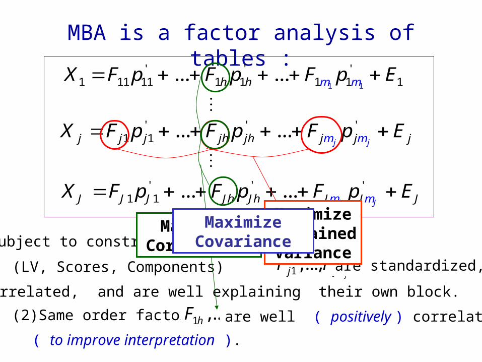
MBA is a factor analysis of tables :

(1) Factors (LV, Scores, Components)

uncorrelated, and are well explaining their own block.

1,..., jj jmF F are standardized,

(2) Same order factors 1 ,...,h JhF F are well ( positively ) correlated

subject to constraints :

1 1

' ' '1 11 11 1 1 1 1 1... ...h mh mX F p F p F p E

' ' '

1 1 ... ...J JJ J J Jh J mJ Jmh JX F p F p F p E

( to improve interpretation ).

MaximizeexplainedVariance

MaximizeCorrelation

MaximizeCovariance

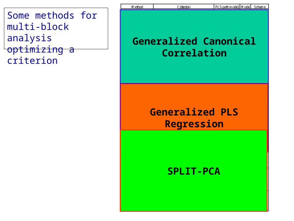
Some methods formulti-block analysisoptimizing a criterion

Method Criterion PLS path model Mode Scheme

(1) SUMCOR (Horst, 1961)

,( , ) j kj k

Max Cor F F

or ( , ) j kj kMax Cor F F

Hierarchical B Centroid

(2) MAXVAR (Horst, 1961) or GCCA (Carroll, 1968)

( , )first j kMax Cor F F (a)

or 2

1( , ) j JjMax Cor F F

Hierarchical B Factorial

(3) SsqCor (Kettenring, 1971)

2

,( , ) j kj k

Max Cor F F Confirmatory B Factorial

(4) GenVar (Kettenring, 1971) det ( , )j kMin Cor F F

(5) MINVAR (Kettenring, 1971) ( , )last j kMin Cor F F (b)

(6) Lafosse (1989) 2 ( , ) j kj k

Max Cor F F

(7) Mathes (1993) or Hanafi (2005) ,

( , ) j kj kMax Cor F F Confirmatory B Centroid

(8) MAXDIFF (Van de Geer, 1984 & Ten Berge, 1988)

1( , )

jj j k kall w j k

Max Cov X w X w

(9) MAXBET (Van de Geer, 1984 & Ten Berge, 1988)

1 ,( , )

jj j k kall w j k

Max Cov X w X w

(10) MAXDIFF B (Hanafi & Kiers, 2006)

2

1( , )

jj j k kall w j k

Max Cov X w X w

(11) (Hanafi & Kiers, 2006)

1( , )

jj j k kall w j k

Max Cov X w X w

(12) ACOM (Chessel & Hanafi, 1996) or Split PCA (Lohmöller, 1989)

21 1 1

( , ) j

j j J Jall w jMax Cov X w X w

or 2

, j

TF p j jj

Min X Fp

Hierarchical A Path-

weighting

(13) Generalized PCA (Casin, 2001)

2 2 ˆ( , ) ( , )j jh jj h

Max

R F X Cor x F (c)

(14) MFA (Escofier & Pagès, 1994)

,

2

1

[ ( , )

jF p

Tj j

j first jh j

Min

X FpCor x x

Hierarchical (applied to the

reduced Xj) (d)

A Path-

weighting

(15) Oblique maximum variance method (Horst, 1965)

,

21/ 21

( )

jF p

T Tj j j j

j

Min

X X X Fpn

Hierarchical (applied to the transformed Xj)

(e)

A Path-

weighting

Generalized CanonicalCorrelation

Generalized PLSRegression

SPLIT-PCA

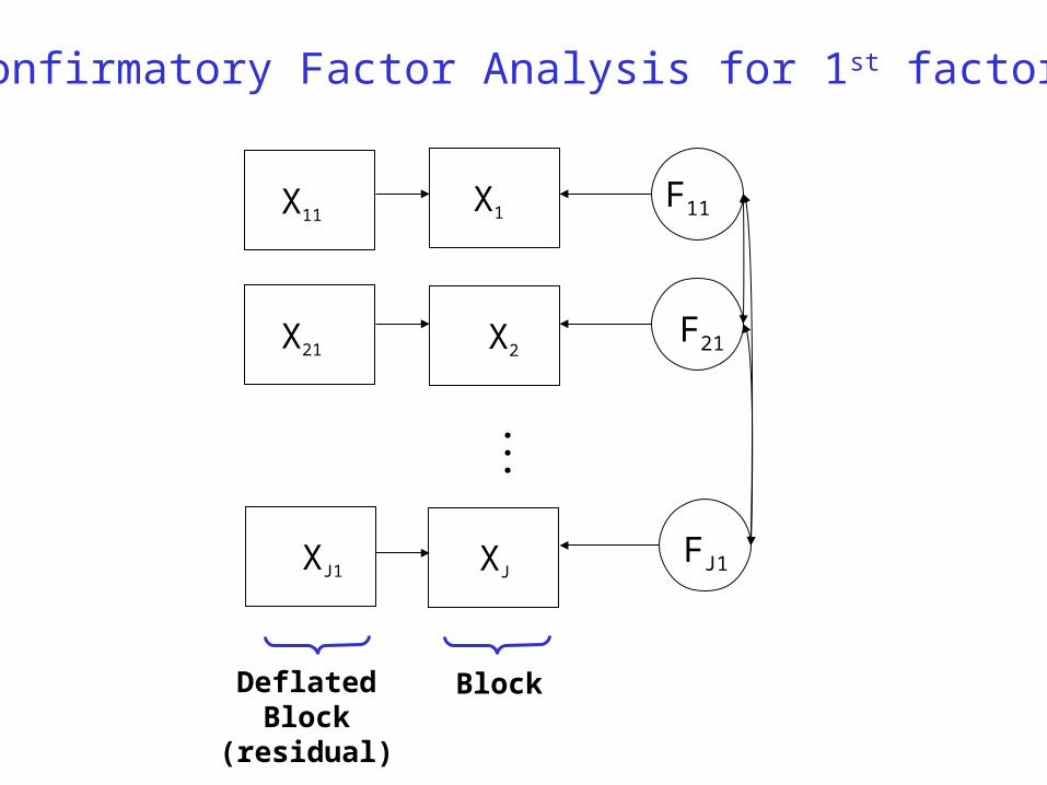
Confirmatory Factor Analysis for 1st factors

X1

X2

XJ

X11

X21

XJ1

F11

F21

FJ1

BlockDeflatedBlock

(residual)

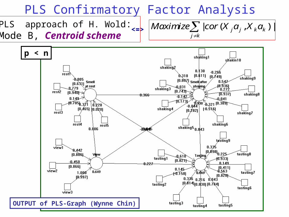
PLS Confirmatory Factor AnalysisPLS approach of H. Wold: Mode B, Centroid scheme

| ( , ) |j j k kj k

Maximize cor X a X a<=>

OUTPUT of PLS-Graph (Wynne Chin)

p < n

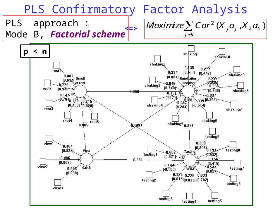
PLS Confirmatory Factor AnalysisPLS approach : Mode B, Factorial scheme

2 ( , )j j k kj k

Maximize Cor X a X a<=>

p < n

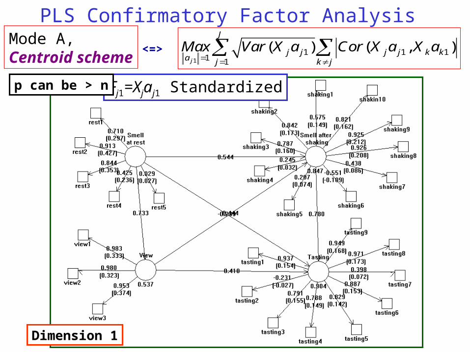
PLS Confirmatory Factor AnalysisMode A,Centroid scheme 1

1 1 11 1

( ) ( , )j

J

j j j j k ka j k j

Max Var X a Cor X a X a <=>

Dimension 1

Fj1=Xjaj1 Standardizedp can be > n

PLS Confirmatory Factor AnalysisMode ACentroid scheme 2

1 2 1 2 1 21 1

( ) ( , )j

J

j j j j k ka j k j

Max Var X a Cor X a X a

Dimension 2

Expressed in term of original variables

<=>

Deflated blockFj2=Xj1aj2 Standardized

S MELL AT RES T

F11

3210-1-2-3

F1

2

4

3

2

1

0

-1

-2

T2

T1

2ING1ROC

2BEA

1BEN1ING

1POY2DAM

PER14EL

1TUR

DO M1

3EL

1BOI2BOU1DAM

1VAU

1FON

1CHA

2EL

F11

3210-1-2-3

F1

2

4

3

2

1

0

-1

-2

T2

T1

2ING1ROC

2BEA

1BEN1ING

1POY2DAM

PER14EL

1TUR

DO M1

3EL

1BOI2BOU1DAM

1VAU

1FON

1CHA

2EL

VI EW

F21

210-1-2-3

F2

2

2.5

2.0

1.5

1.0

.5

0.0

-.5

-1.0

-1.5

-2.0

-2.5

T2

T1

2ING

1ROC

2BEA

1BEN

1ING

1POY

2DAM

PER1

4EL1TUR

DO M1

3EL

1BOI 2BOU

1DAM

1VAU

1FON1CHA

2EL

F21

210-1-2-3

F2

2

2.5

2.0

1.5

1.0

.5

0.0

-.5

-1.0

-1.5

-2.0

-2.5

T2

T1

2ING

1ROC

2BEA

1BEN

1ING

1POY

2DAM

PER1

4EL1TUR

DO M1

3EL

1BOI 2BOU

1DAM

1VAU

1FON1CHA

2EL

S MELL AFTER S HAK I NG

F31

210-1-2-3

F3

2

3

2

1

0

-1

-2

T2 T1

2ING

1ROC

2BEA

1BEN

1ING

1POY2DAM

PER1 4EL

1TUR

DO M1

3EL

1BOI

2BOU

1DAM

1VAU

1FON

1CHA2EL

F31

210-1-2-3

F3

2

3

2

1

0

-1

-2

T2 T1

2ING

1ROC

2BEA

1BEN

1ING

1POY2DAM

PER1 4EL

1TUR

DO M1

3EL

1BOI

2BOU

1DAM

1VAU

1FON

1CHA2EL

TAS TI NG

F41

210-1-2-3-4

F4

2

3.5

3.0

2.5

2.0

1.5

1.0

.5

0.0

-.5

-1.0

-1.5

T2

T1

2ING

1ROC2BEA

1BEN

1ING

1PO Y

2DAM

PER1

4EL

1TURDOM1

3EL1BOI

2BOU

1DAM

1VAU

1FON1CHA 2EL

F41

210-1-2-3-4

F4

2

3.5

3.0

2.5

2.0

1.5

1.0

.5

0.0

-.5

-1.0

-1.5

T2

T1

2ING

1ROC2BEA

1BEN

1ING

1PO Y

2DAM

PER1

4EL

1TURDOM1

3EL1BOI

2BOU

1DAM

1VAU

1FON1CHA 2EL

PLS-CFA: Visualization of wine variability among the blocks

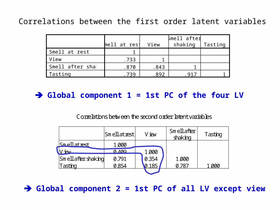
1

.733 1

.870 .843 1

.739 .892 .917 1

Smell at rest

View

Smell after shaking

Tasting

Smell at rest ViewSmell after

shaking Tasting

Correlations between the first order latent variables

Global component 1 = 1st PC of the four LV

Correlations between the second order latent variables

Smell at rest View Smell after

shaking Tasting

Smell at rest 1.000 View 0.409 1.000 Smell after shaking 0.791 0.354 1.000 Tasting 0.854 0.185 0.787 1.000

Global component 2 = 1st PC of all LV except view

Mapping of the correlations with the global components

Correlation with global component 1

1.0.8.6.4.2-.0-.2-.4-.6

Cor

rela

tion

with

glob

al c

ompo

nent

21.0

.8

.6

.4

.2

-.0

-.2

-.4

-.6

GLOBAL QUALITY

Harmony

Ending intensityin mouth

Bitterness

Mellowness

Balance

Alcohol

Astringency

Acidity

Intensity of attack

Aromatic qualityin mouth

Aromatic persistence

Aromatic intensityin mouth

Phelonic note

Vegetable note Spicy note

Floral note

Fruity note

Smell quality

Smell intensity

Surface impression

Shading

Visual intensity

Spicy note at rest

Floral noteat rest

Fruity noteat rest

Aromatic quality at rest

Smell intensity atrest

Correlation with global component 1

1.0.8.6.4.2-.0-.2-.4-.6

Cor

rela

tion

with

glo

bal c

ompo

nent

2

1.0

.8

.6

.4

.2

-.0

-.2

-.4

-.6

GLOBAL QUALITY

Harmony

Ending intensityin mouth

Bitterness

Mellowness

Balance

Alcohol

Astringency

Acidity

Intensity of attack

Aromatic qualityin mouth

Aromatic persistence

Aromatic intensityin mouth

Phelonic note

Vegetable note Spicy note

Floral note

Fruity note

Smell quality

Smell intensity

Surface impression

Shading

Visual intensity

Spicy note at rest

Floral noteat rest

Fruity noteat rest

Aromatic quality at rest

Smell intensity atrest

Wine visualization in the global component spaceWines marked by Appellation

Global component 1

210-1-2-3

Glo

ba

l co

mp

on

en

t 2

3.5

3.0

2.5

2.0

1.5

1.0

.5

0.0

-.5

-1.0

-1.5

Appellation

Saumur

Chinon

Bourgueil

T2

T1

2ING 1ROC

2BEA

1BEN1ING

1POY

2DAM

PER14EL

1TURDOM1

3EL

1BOI2BOU 1DAM

1VAU

1FON

1CHA 2EL

GOOD QUALITY

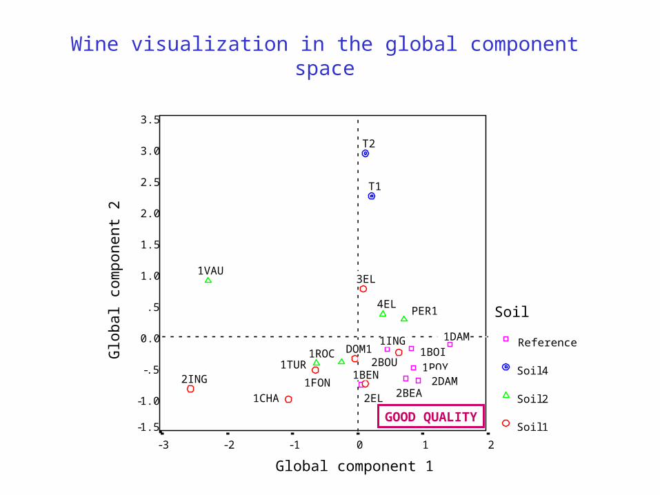
Wine visualization in the global component space

Wines marked by Soil

Global component 1

210-1-2-3

Glo

bal c

ompo

nent

23.5

3.0

2.5

2.0

1.5

1.0

.5

0.0

-.5

-1.0

-1.5

Soil

Reference

Soil 4

Soil 2

Soil 1

T2

T1

2ING

1ROC

2BEA

1BEN

1ING

1POY2DAM

PER14EL

1TURDOM1

3EL

1BOI2BOU

1DAM

1VAU

1FON

1CHA 2EL

Global component 1

210-1-2-3

Glo

bal c

ompo

nent

23.5

3.0

2.5

2.0

1.5

1.0

.5

0.0

-.5

-1.0

-1.5

Soil

Reference

Soil 4

Soil 2

Soil 1

T2

T1

2ING

1ROC

2BEA

1BEN

1ING

1POY2DAM

PER14EL

1TUR

DOM1

3EL

1BOI2BOU

1DAM

1VAU

1FON

1CHA 2EL

GOOD QUALITY

210-1-2-3

3

2

1

0

-1

-2

GLOBAL SCORE

Tasting

Smell after shaking

View

Smell at rest2BEA

T1

1POY3EL

1CHA

1VAU

Visualization of wine variability among the blocksStar-plots of scores for some wines

2,01,00,0-1,0-2,0-3,0

3,0

2,0

1,0

0,0

-1,0

-2,0

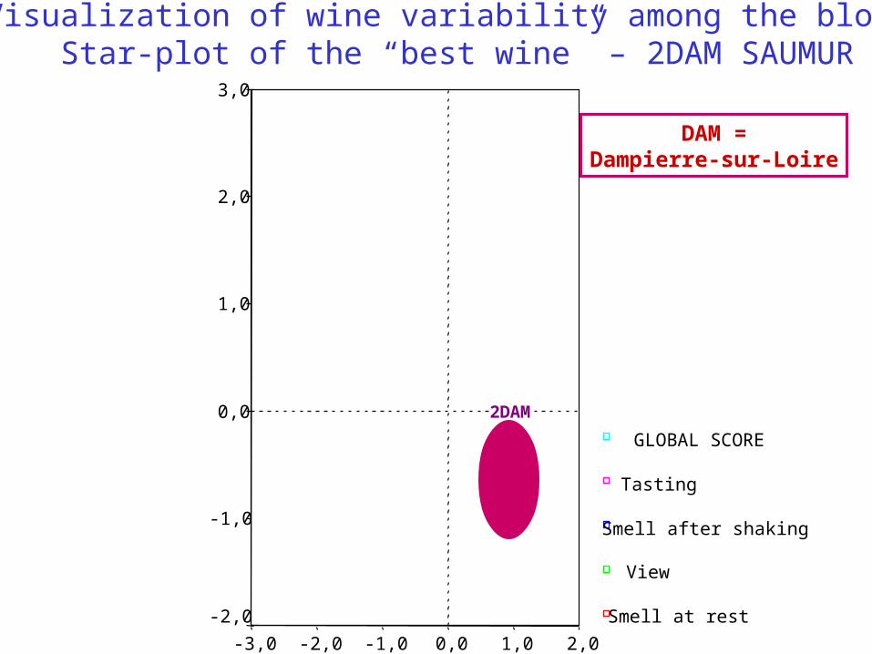
GLOBAL SCORE

Tasting

Smell after shaking

View

Smell at rest

2DAM

Visualization of wine variability among the blocksStar-plot of the “best wine” – 2DAM SAUMUR

DAM =Dampierre-sur-Loire

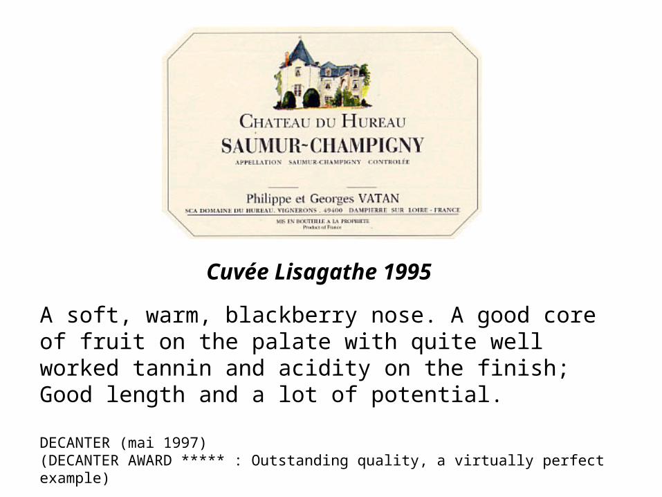
A soft, warm, blackberry nose. A good core of fruit on the palate with quite well worked tannin and acidity on the finish; Good length and a lot of potential.

DECANTER (mai 1997)(DECANTER AWARD ***** : Outstanding quality, a virtually perfect example)

Cuvée Lisagathe 1995

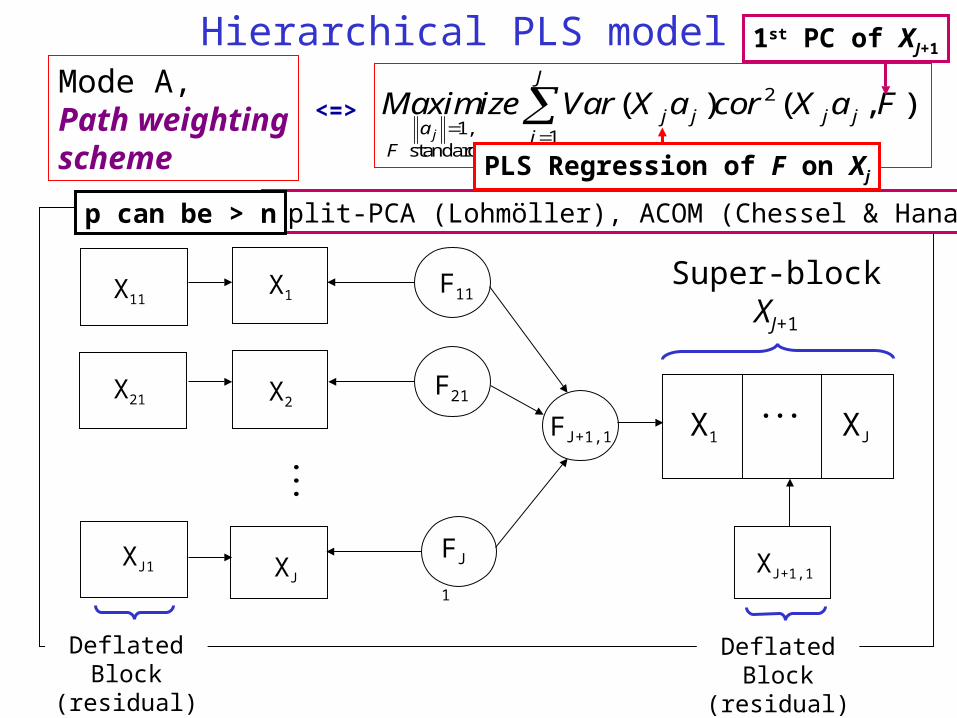
Hierarchical PLS modelMode A, Path weightingscheme

2

1, 1 standardized

( ) ( , ) j

J

j j j ja j

F

Maximize Var X a cor X a F

<=>

X1

X2

XJ

X11

X21

XJ1

F11

F21

FJ1

X1 XJ

FJ+1,1

XJ+1,1

Super-blockXJ+1

Split-PCA (Lohmöller), ACOM (Chessel & Hanafi)

1st PC of XJ+1

PLS Regression of F on Xj

p can be > n

DeflatedBlock

(residual)

DeflatedBlock

(residual)

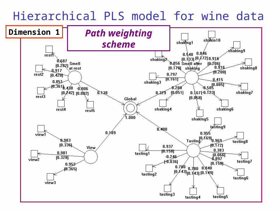
Hierarchical PLS model for wine dataDimension 1 Path weighting scheme

Hierarchical PLS model for wine dataDimension 2 Path weighting scheme

Other results for Hierarchical PLS ( p < n )

Mode B, Centroid scheme SUMCOR (Horst, 1961)

, ,

( , ) or ( , ) j j k k j jj k j k

Max Cor X a X a Max Cor X a F

Mode B, Factorial scheme GCCA (Carroll, 1968)

2

,

( , ) j jj k

Max Cor X a F

Multiblock and Hierarchical PLS

p can be > n p must be < n

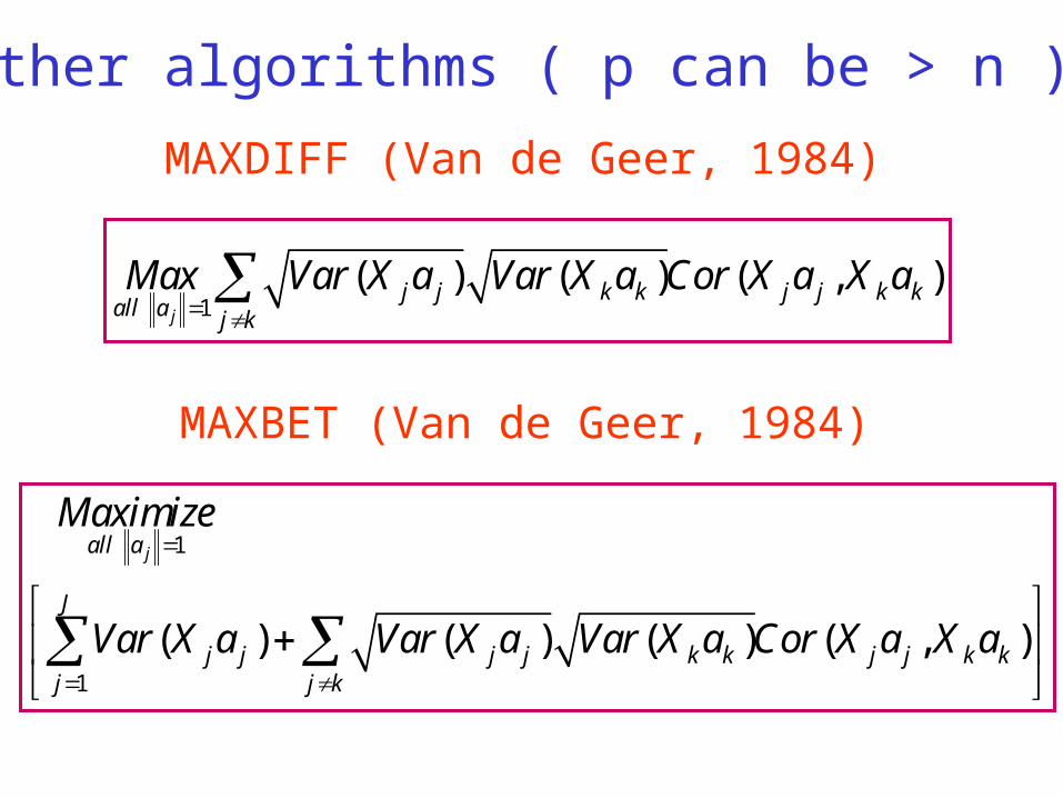
MAXDIFF (Van de Geer, 1984)

1( ) ( ) ( , )

jj j k k j j k k

all a j k

Max Var X a Var X a Cor X a X a

MAXBET (Van de Geer, 1984)

1

1

( ) ( ) ( ) ( , )

jall a

J

j j j j k k j j k kj j k

Maximize

Var X a Var X a Var X a Cor X a X a

Other algorithms ( p can be > n )

Very high dimensional data

• For very high dimensional data (p >> n), the blocks can be replaced by their principal components.

• All the algorithms using the covariance criterion (Mode A or PLS regression) can be used on the original data or on the principal components and yield to exactly the same latent variables Fjh.

Multiblock analysis and PLS approach

Conclusion

On the wine data, all these algorithmsgive very close results.

PLS path modeling appears to bea unified frame for Multi-block dataanalysis.

Final Conclusion

Try PLS Regression and PLS Path modeling.

The proof of the pudding is in the eating.

PLS’07 Ås, Norway, August 2007

Back to the origin