unit2 - uampopia.ft.uam.es/aknebe/page3/files/computacion/unit2.pdf ·...
TRANSCRIPT
A/Prof. Alexander Knebe
Unit 2
Matrices and Advanced Plo7ng/Scrip;ng
Computa;onal Physics I Unit 2

A/Prof. Alexander Knebe
! every variable in MATLAB is a matrix >> a=1 1x1 matrix >> b=[1, 2] 1x2 matrix >> c=[1; 2] 2x1 matrix >> d=[1, 2; 3, 4] 2x2 matrix >> A=[10, -3, 7; 2, 12, 0] 2x3 matrix
A(n,m) n=rown, m=column
" exercise:
• define various matrices (1x1, 1x3, 3x1, 3x3) and check the results of…
>> transpose(d)>>d’
>> size(d) >> diag(d)
• Note that diag() can extract and generate diagonal matrix elements! • use help to learn about the commands diag(), zeros(), eye(), ones(), numel()
! matrix mul;plica;on:
• A(n,m) * B(m,k) = C(n,k) mathema;cal• A(n,m) .* B(n,m) = C(n,m) component-‐wise
" exercise:
• perform the following opera;ons on A=[1,2;3,4] and B=[5,6;7,8]
>> A+B >> A-B >> A*B >> A.*B >> A./B
• Note: the opera;ons A/B and A\B will be explained later!
" exercise:
• use A and B from the previous exercise to generate the following matrix C with one command
>> C = ??? C = 1 2 0 0
3 4 0 0 0 0 5 6 0 0 7 8
MATLAB matrices
Computa;onal Physics I Unit 2
€
A =A(1,1) A(1,2) A(1,3)A(2,1) A(2,2) A(2,3)"
# $
%
& '
Day 1
A/Prof. Alexander Knebe
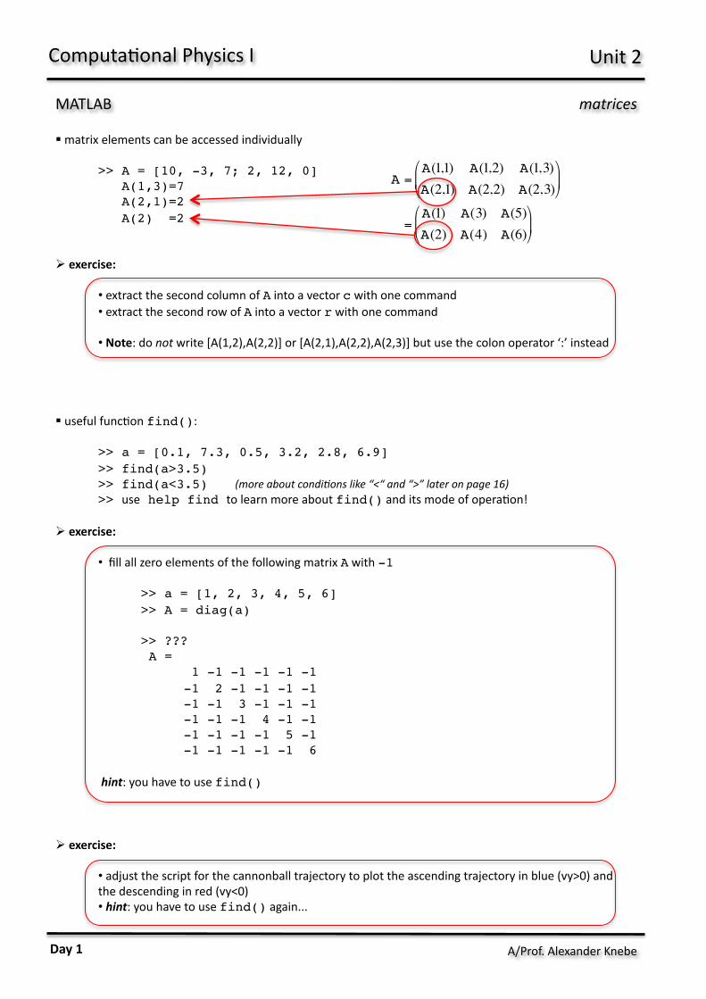
! matrix elements can be accessed individually
>> A = [10, -3, 7; 2, 12, 0] A(1,3)=7 A(2,1)=2 A(2) =2
" exercise:
• extract the second column of A into a vector c with one command• extract the second row of A into a vector r with one command
• Note: do not write [A(1,2),A(2,2)] or [A(2,1),A(2,2),A(2,3)] but use the colon operator ‘:’ instead
! useful func;on find():
>> a = [0.1, 7.3, 0.5, 3.2, 2.8, 6.9]>> find(a>3.5)>> find(a<3.5) >> use help find to learn more about find() and its mode of opera;on!
" exercise:
• fill all zero elements of the following matrix A with -1
>> a = [1, 2, 3, 4, 5, 6]>> A = diag(a)
>> ??? A =
1 -1 -1 -1 -1 -1-1 2 -1 -1 -1 -1-1 -1 3 -1 -1 -1-1 -1 -1 4 -1 -1-1 -1 -1 -1 5 -1-1 -1 -1 -1 -1 6
hint: you have to use find()
" exercise:
• adjust the script for the cannonball trajectory to plot the ascending trajectory in blue (vy>0) and the descending in red (vy<0) • hint: you have to use find() again...
€
A =A(1,1) A(1,2) A(1,3)A(2,1) A(2,2) A(2,3)"
# $
%
& '
=A(1) A(3) A(5)A(2) A(4) A(6)"
# $
%
& '
MATLAB matrices
Computa;onal Physics I Unit 2
(more about condi0ons like “<“ and “>” later on page 16)
Day 1

A/Prof. Alexander Knebe
! the rota;on of a 2D vector can be described by a matrix opera;on
! the matrix M is determined as follows:
€
! v rotated = ˆ M ! v
MATLAB rota0on via matrices
Computa;onal Physics I Unit 2
€
! v rotated =vxrotated
vyrotated
"
# $
%
& '
€
! v =vx
vy
"
# $
%
& '
€
ϕ
€
β
€
α€
vx = v cosα ; vxrotated = v cosβ ; β = α +ϕ
vy = v sinα ; vyrotated = v sinβ
€
vxrotated = v cos(α +ϕ) = v cosα cosϕ − sinα sinϕ[ ] = vx cosϕ − vy sinϕ
vyrotated = v sin(α +ϕ) = v sinα cosϕ + cosα sinϕ[ ] = vy cosϕ + vx sinϕ
=> =>
€
ˆ M =cosϕ −sinϕsinϕ cosϕ$
% &
'
( )
" exercise:
• write a script that rotates a given 2D vector about a pre-‐defined angle (given in degrees!) using the rota;on matrix • proof that the original and rotated vectors have the same norm. • graphically display the two vectors using the MATLAB func;on quiver()
! the rota;on of a 3D vector can be described by successive matrix opera;ons
€
Mx =
1 0 00 cosϕ −sinϕ0 sinϕ cosϕ
$
%
& & &
'
(
) ) )
€
My =
cosϕ 0 −sinϕ0 1 0sinϕ 0 cosϕ
$
%
& & &
'
(
) ) )
€
Mz =
cosϕ −sinϕ 0sinϕ cosϕ 00 0 1
$
%
& & &
'
(
) ) )
rota;on about x-‐axis rota;on about y-‐axis rota;on about z-‐axis
" exercise:
• write a script that rotates a given 3D vector about two pre-‐defined angles (given in degrees!), i.e. one rota;on about the x-‐axis and another rota;on about the z-‐axis. • show that rota;ons are non-‐permuta;ve, i.e. first rota;ng about the x-‐ and then the z-‐axis is not the same as first rota;ng about the z-‐ and then the x-‐axis. • proof that all (rotated) vectors have the same norm. • graphically display all vectors using the MATLAB func;on quiver3()
Day 1
" exercise:
• write a script that rotates x = sin(t) (for t∈[0,2π]) about 32o • hints:
• put the vectors t() and x() into a matrix S=[t; x]• rotate that matrix via R*S where R is the rota;on matrix • extract the new vectors t() and x() from the rotated matrix and plot them

A/Prof. Alexander Knebe
MATLAB
! we intend to visualize a func;on of mul;ple variables, e.g.
f(x,y) = x2 + y2 with
• now we need to generate a 2D mesh of points:
>> xm = linspace(a,b,N)>> ym = linspace(c,d,M)>> [x,y] = meshgrid(xm,ym)
both x and y are matrices of dimension MxN:
x = y =
• the 2D mesh covered by x and y can then be used to calculate f(x,y), i.e. generate another MxN matrix that contains the func;on values
>> f = x.^2+y.^2 f =
• the matrix f() can then be visualized using one of the following MATLAB func;ons:
>> contour(x,y,f) >> mesh(x,y,f)>> surf(x,y,f)>> surfc(x,y,f)>> surfl(x,y,f)
" exercise:
• write a script x2+y2.m that plots f(x,y)=x2+y2 within the range [-‐100,100]x[-‐100,100] • use subplot() or figure() to view all possible contours and surfaces simultaneously • use colorbar, axis, and shading to modify the figure• use help to find out more about mesh(), waterfall(), surf(), surfc(), surfl()• use help to learn more about colorbar, axis, shading
" exercise:
• write a script sinxcosx.m that visualizes f(x,y)=sin(x)cos(y) within the range [0,2π]x[0,2π]
plo=ng scalar fields
Computa;onal Physics I Unit 2
€
a
€
b
€
c
€
d
€
M = 3
€
x ∈[a,b]y ∈[c,d]
€
N = 5
a ... ... ... b
a ... ... ... b
a ... ... ... b
c c c c c
... ... ... ... ...
d d d d d
f(a,c) ... ... ... f(b,c)
... ... ... ... ...
f(a,d) ... ... ... f(b,d)
Day 1
A/Prof. Alexander Knebe
MATLAB
" exercise:
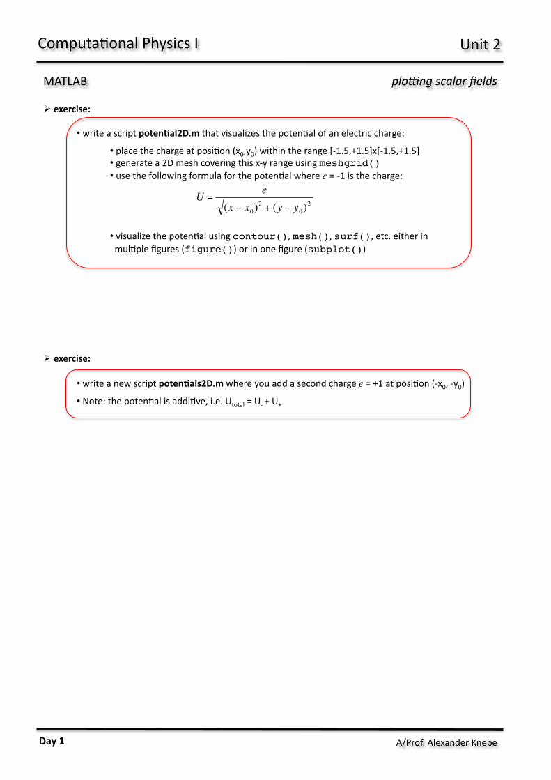
• write a script poten<al2D.m that visualizes the poten;al of an electric charge:
• place the charge at posi;on (x0,y0) within the range [-‐1.5,+1.5]x[-‐1.5,+1.5] • generate a 2D mesh covering this x-‐y range using meshgrid()• use the following formula for the poten;al where e = -‐1 is the charge:
• visualize the poten;al using contour(), mesh(), surf(), etc. either in mul;ple figures (figure()) or in one figure (subplot())
" exercise:
• write a new script poten<als2D.m where you add a second charge e = +1 at posi;on (-‐x0, -‐y0)
• Note: the poten;al is addi;ve, i.e. Utotal = U-‐ + U+
plo=ng scalar fields
€
U =e
(x − x0)2 + (y − y0)
2
Computa;onal Physics I Unit 2
Day 1
A/Prof. Alexander Knebe
MATLAB
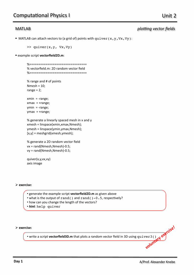
! MATLAB can aaach vectors to (a grid of) points with quiver(x,y,Vx,Vy):
>> quiver(x,y, Vx,Vy)
! example script vectorfield2D.m:
%================================ % vectorfield.m: 2D random vector field %================================
% range and # of points Nmesh = 10; range = 2;
xmin = -‐range; xmax = +range; ymin = -‐range; ymax = +range;
% generate a linearly spaced mesh in x and y xmesh = linspace(xmin,xmax,Nmesh); ymesh = linspace(ymin,ymax,Nmesh); [x,y] = meshgrid(xmesh,ymesh);
% generate a 2D random vector field vx = rand(Nmesh,Nmesh)-‐0.5; vy = rand(Nmesh,Nmesh)-‐0.5;
quiver(x,y,vx,vy) axis image
" exercise:
• generate the example script vectorfield2D.m as given above • what is the output of rand() and rand()-0.5, respec;vely? • how can you change the length of the vectors? • hint: help quiver
" exercise:
• write a script vectorfield3D.m that plots a random vector field in 3D using quiver3()
plo=ng vector fields
Computa;onal Physics I Unit 2
Day 1

A/Prof. Alexander Knebe
MATLAB
! recall the exercises on numerical deriva;ves, e.g. the calcula;on of dx and df for df/dx
>> il = [1:N-1], ir = [2:N];>> dx = x[ir]-x[il];>> df = f[ir]-f[il];
! as this is a rather important opera;on MATLAB has a simple command for this that does not need the index vectors:
>> dx = diff(x);>> df = diff(f);
" exercise:
• adjust your deriva<on.m scipt to now use diff() instead of index vectors
! for func;ons of mul;ple variables we have deriva;ves with respect to every variable, e.g. the force is the gradient of the poten;al:
! MATLAB can calculate the gradient of a given scalar field
>> [Fx, Fy] = gradient(U) 2D gradient>> [Fx, Fy, Fz] = gradient(U) 3D gradient
" exercise:
• write a new script force2D.m by adjus;ng poten<al2D.m that now plots the force field.
" exercise:
• write a script force3D.m that now plots the 3D force field of the same electric charge
• hint: you now need to add a 3rd dimension (i.e. z) to all calcula;ons including meshgrid(), the actual poten;al and the gradient.
gradients
€
! F = −
! ∇ U = −
∂U∂x, ∂U∂y, ∂U∂z
%
& '
(
) *
Computa;onal Physics I Unit 2
Day 1
A/Prof. Alexander Knebe
MATLAB
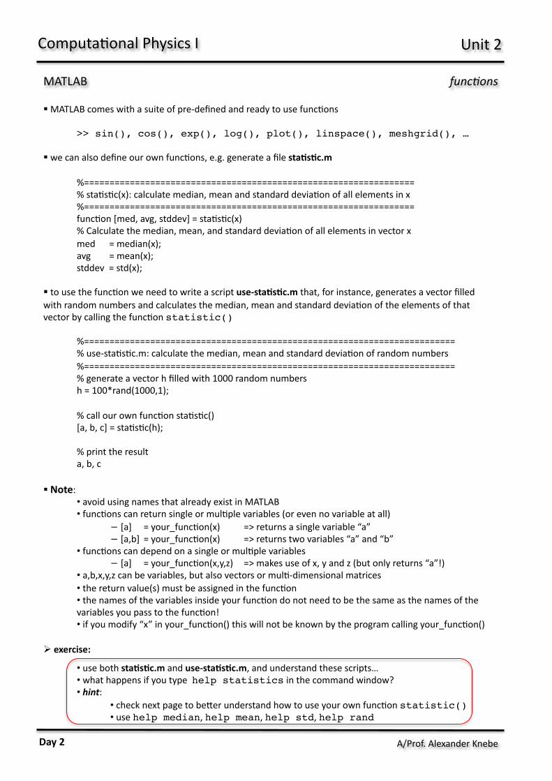
! MATLAB comes with a suite of pre-‐defined and ready to use func;ons
>> sin(), cos(), exp(), log(), plot(), linspace(), meshgrid(), … ! we can also define our own func;ons, e.g. generate a file sta<s<c.m
%================================================================= % sta;s;c(x): calculate median, mean and standard devia;on of all elements in x
%================================================================= func;on [med, avg, stddev] = sta;s;c(x) % Calculate the median, mean, and standard devia;on of all elements in vector x med = median(x); avg = mean(x); stddev = std(x);
! to use the func;on we need to write a script use-‐sta<s<c.m that, for instance, generates a vector filled with random numbers and calculates the median, mean and standard devia;on of the elements of that vector by calling the func;on statistic()
%========================================================================= % use-‐sta;s;c.m: calculate the median, mean and standard devia;on of random numbers
%========================================================================= % generate a vector h filled with 1000 random numbers h = 100*rand(1000,1); % call our own func;on sta;s;c() [a, b, c] = sta;s;c(h); % print the result a, b, c
! Note: • avoid using names that already exist in MATLAB • func;ons can return single or mul;ple variables (or even no variable at all)
− [a] = your_func;on(x) => returns a single variable “a” − [a,b] = your_func;on(x) => returns two variables “a” and “b”
• func;ons can depend on a single or mul;ple variables − [a] = your_func;on(x,y,z) => makes use of x, y and z (but only returns “a”!)
• a,b,x,y,z can be variables, but also vectors or mul;-‐dimensional matrices • the return value(s) must be assigned in the func;on • the names of the variables inside your func;on do not need to be the same as the names of the variables you pass to the func;on! • if you modify “x” in your_func;on() this will not be known by the program calling your_func;on()
" exercise:
• use both sta<s<c.m and use-‐sta<s<c.m, and understand these scripts… • what happens if you type help statistics in the command window? • hint:
• check next page to beaer understand how to use your own func;on statistic()• use help median, help mean, help std, help rand
func0ons
Computa;onal Physics I Unit 2
Day 2

A/Prof. Alexander Knebe
MATLAB
! before being able to use a func;on you must tell MATLAB where that func;on can be found:
func0ons
Computa;onal Physics I Unit 2
1. click “Set Path...”
2. “Add Folder...” and select the folder where your your_func<on.m files is located
3. “Save” to save the changes you just made
Day 2

A/Prof. Alexander Knebe
MATLAB
" exercise:
• write a script use-‐oplot.m that calls your own func;on oplot(x,y) defined in oplot.m • your func;on oplot() is supposed to “overplot” some data (x,y) in an exis;ng plot, e.g.
%================================================================= % use-‐oplot.m: plot two func;ons in the same figure using oplot()
%================================================================= x = linspace(0,2*pi,100); plot(x,sin(x)) % use MATLAB’s built-‐in func;on plot() to ini;ate the plot oplot(x,cos(x)) % use your own func;on oplot() to add another curve to the plot
• hints:
• remember hold on and hold off • the func;on oplot() does not return anything!
" exercise:
• write a script use-‐ang2rad.m that calls your own func;on ang2rad(x) defined in ang2rad.m conver;ng degrees to radians
• use this func;on to plot a full period of sin(x)
" exercise:
• write a new script force2D-‐dist2D.m by adjus;ng your script force2D.m to now u;lize a func;on dist2D() that calculates
• hint: dist2D() has to accept 4 arguments (x,y,x0,y0) and return 1 result (the distance)
func0ons
€
dist2D = (x − x0)2 + (y − y0)
2
Computa;onal Physics I Unit 2
Day 2

A/Prof. Alexander Knebe
MATLAB
! there are two different types of func<ons in MATLAB:
• script func;ons
function [I] = integrate(g, x0, xend, N)
• anonymous func;ons
g = @(x)(x.^2-exp(-x)) 1) script func<ons:
• script func;ons require you to write an m-‐file with the same name as the func;on • script func;ons can return mul;ple values of different types, e.g.
function [E,V] = ElectricFields(r) where
E is a 3-‐component vector (electric field), V is a 1-‐component scalar (poten;al field), and r the 3-‐component vector (3D posi;on of electric charge)
• all variables declared as return values must be set inside the func;on • a script func;on can be a block of certain opera;ons that you plan to do repeatedly, e.g.
func0ons
Computa;onal Physics I
integrate(): integrate the func;on g(x) from x0 to xend in N steps
and return its value.
(g,x0,xend,N) [I]
input output
Unit 2
Day 2
A/Prof. Alexander Knebe
MATLAB
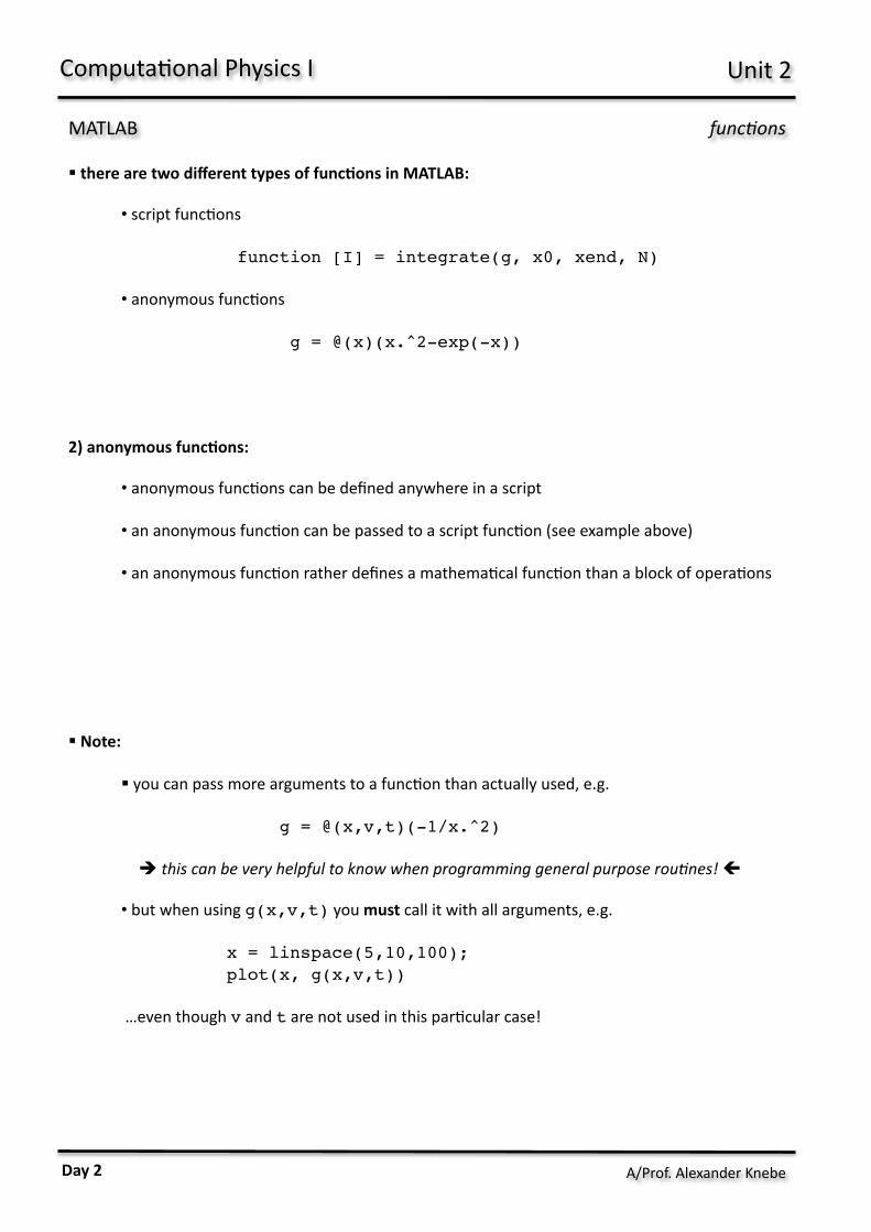
! there are two different types of func<ons in MATLAB:
• script func;ons
function [I] = integrate(g, x0, xend, N)
• anonymous func;ons
g = @(x)(x.^2-exp(-x))
2) anonymous func<ons:
• anonymous func;ons can be defined anywhere in a script • an anonymous func;on can be passed to a script func;on (see example above) • an anonymous func;on rather defines a mathema;cal func;on than a block of opera;ons
! Note:
! you can pass more arguments to a func;on than actually used, e.g.
g = @(x,v,t)(-1/x.^2)
# this can be very helpful to know when programming general purpose rou0nes! $% • but when using g(x,v,t) you must call it with all arguments, e.g.
x = linspace(5,10,100);plot(x, g(x,v,t))
…even though v and t are not used in this par;cular case!
func0ons
Computa;onal Physics I Unit 2
Day 2
A/Prof. Alexander Knebe Dr. Alexander Knebe
MATLAB
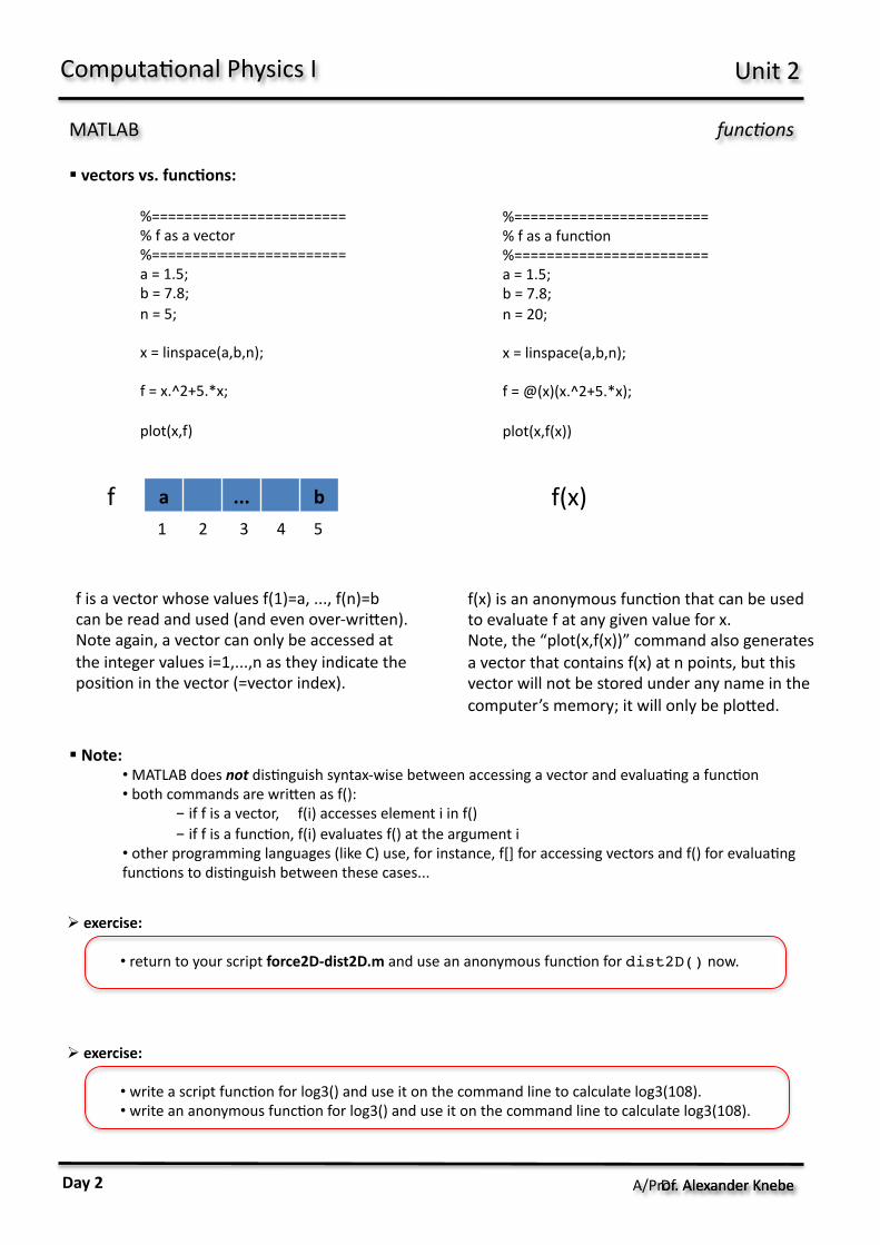
! vectors vs. func<ons:
func0ons
Computa;onal Physics I Unit 2
%======================== % f as a vector
%======================== a = 1.5; b = 7.8; n = 5; x = linspace(a,b,n); f = x.^2+5.*x; plot(x,f)
%======================== % f as a func;on
%======================== a = 1.5; b = 7.8; n = 20; x = linspace(a,b,n); f = @(x)(x.^2+5.*x); plot(x,f(x))
a ... b f f(x) 1 2 3 4 5
f is a vector whose values f(1)=a, ..., f(n)=b can be read and used (and even over-‐wriaen). Note again, a vector can only be accessed at the integer values i=1,...,n as they indicate the posi;on in the vector (=vector index).
f(x) is an anonymous func;on that can be used to evaluate f at any given value for x. Note, the “plot(x,f(x))” command also generates a vector that contains f(x) at n points, but this vector will not be stored under any name in the computer’s memory; it will only be ploaed.
" exercise:
• return to your script force2D-‐dist2D.m and use an anonymous func;on for dist2D() now.
" exercise:
• write a script func;on for log3() and use it on the command line to calculate log3(108). • write an anonymous func;on for log3() and use it on the command line to calculate log3(108).
! Note: • MATLAB does not dis;nguish syntax-‐wise between accessing a vector and evalua;ng a func;on • both commands are wriaen as f():
- if f is a vector, f(i) accesses element i in f() - if f is a func;on, f(i) evaluates f() at the argument i
• other programming languages (like C) use, for instance, f[] for accessing vectors and f() for evalua;ng func;ons to dis;nguish between these cases...
Day 2
A/Prof. Alexander Knebe
MATLAB
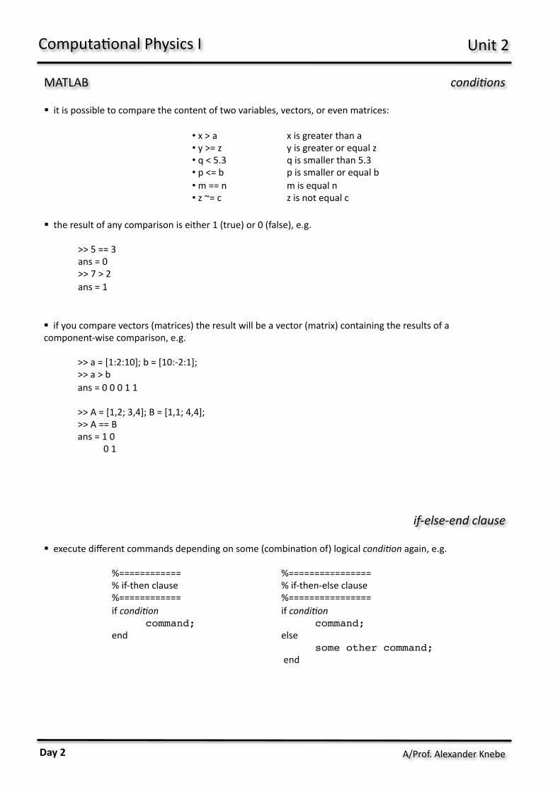
! execute different commands depending on some (combina;on of) logical condi0on again, e.g.
%============ %================ % if-‐then clause % if-‐then-‐else clause
%============ %================ if condi0on if condi0on
command; command;end else
some other command; end
condi0ons
Computa;onal Physics I Unit 2
Day 2
if-‐else-‐end clause
• x > a x is greater than a • y >= z y is greater or equal z • q < 5.3 q is smaller than 5.3 • p <= b p is smaller or equal b • m == n m is equal n • z ~= c z is not equal c
! it is possible to compare the content of two variables, vectors, or even matrices:
! the result of any comparison is either 1 (true) or 0 (false), e.g.
>> 5 == 3 ans = 0 >> 7 > 2 ans = 1
! if you compare vectors (matrices) the result will be a vector (matrix) containing the results of a component-‐wise comparison, e.g.
>> a = [1:2:10]; b = [10:-‐2:1]; >> a > b ans = 0 0 0 1 1 >> A = [1,2; 3,4]; B = [1,1; 4,4]; >> A == B ans = 1 0 0 1

A/Prof. Alexander Knebe
MATLAB
Computa;onal Physics I Unit 2
Day 2
" exercise:
• write a script cannonball-‐maximum.m by adjus;ng the cannonball.m script to also calculate the maximum height ymax of the cannonball • how long does it take to reach this height (i.e. calculate the corresponding tmax, too)? • at what x-‐posi;on xmax does the cannonball reach this height? • generate a plot that indicates the maximum by red lines on top of the actual trajectory:
• hints: • use the following idea to finding the maximum in vector y():
for increasing values of y() the difference between two neighbouring points in y() is greater than zero and less than zero for decreasing values of y(); further, remember the usage of find().
" exercise:
• write a script sine-‐posi<ve.m by adjus;ng sine.m that sets all nega;ve values of sin() to zero.
• hints: • this exercise does note require an if-‐statement • you should remember the usage of find()
0 1 2 3 4 5 6 7 80.9
1
1.1
1.2
1.3
1.4
1.5
1.6
1.7
1.8
x
y
if-‐else-‐end clause

A/Prof. Alexander Knebe
MATLAB
while-‐loops
Computa;onal Physics I Unit 2
! you want to repeat a certain opera;on while some logical condi;on remains true:
while condi0on command;
end
! possible condi0ons are again • > greater than • >= greater or equal • < smaller than • <= smaller or equal • == equal • ~= not equal
! example: we want to determine how oren a number can be divided by 2
%====================================== % simple log2() func;on %====================================== f = 32 n = 0; while f > 1 f = f / 2; n = n + 1; end 2^n
! Note: as the ;tle of the script suggests, this is a very simple (and crude!) form for calcula;ng n=log2(f)
" exercise:
• use the above idea to write a script that evaluates log3() for several values of f (e.g. 27, 243, 531411) and compare to the real log3(f)
Day 2/3
! Note: never compare floa;ng variables (i.e. real numbers) using == or ~= ; use the following instead:
do not use: x==a instead use: abs(x-a) < e for ‘is equal’ do not use: x~=a instead use: abs(x-a) > e for ‘is not equal’
where e defines your desired accuracy, e.g.
will not work will work if tan(0.7) == sin(0.7)/cos(0.7) if abs(tan(0.7)-‐sin(0.7)/cos(0.7)) < 1e-‐10 disp(‘success’) disp(‘success’) end end
(check help disp to learn more about disp())
if-‐else-‐end clause

A/Prof. Alexander Knebe
MATLAB while-‐loops
Computa;onal Physics I Unit 2
" exercise:
• write a script that evaluates whether or not a natural number is a prime number.
• hints: • a prime number is a number that can only be divided by 1 and by itself • use mod(n,div) or rem(n,div) to evaluate the remainder of the division n/div • if rem(n,div)==0 for any 1<div<n then n cannot be a prime number • you must remember the usage of if-else-end
• advanced scrip0ng hints: • use input() to let the user input the natural number:
n = input(‘give a natural number n = ’)
• use disp() to print whether or not n is a prime number: if your_condi0on_for_prime_number
disp(‘prime number’)else
disp(‘not a prime number’)end
! logical condi;ons can be combined:
& : condi;on #1 AND condi;on #2 are true | : condi;on #1 OR condi;on #2 is true
" exercise:
• re-‐write the prime number script using combina;ons of logical expressions, e.g. the while-‐loop condi;on should test for both the remainder of the division and the maximal allowed divisor.
Day 3
A/Prof. Alexander Knebe
MATLAB for-‐loops
Computa;onal Physics I Unit 2
€
fn = fn−1 + fn−2
€
f1 =1 , f2 =1
" exercise:
• write a script fibonacci.m that calculates the first N Fibonacci numbers using a for-‐loop • show in the same script that Binet’s formula for the Fibonacci numbers is correct:
with
€
fn =ϕn −ψ n
5
€
ϕ =1+ 52
,ψ =1− 52
Day 3
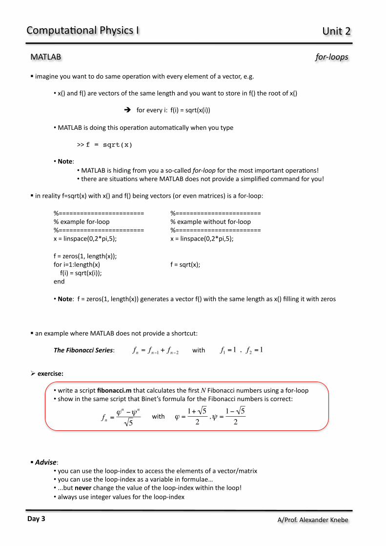
! imagine you want to do same opera;on with every element of a vector, e.g.
• x() and f() are vectors of the same length and you want to store in f() the root of x()
# for every i: f(i) = sqrt(x(i)) • MATLAB is doing this opera;on automa;cally when you type
>> f = sqrt(x) • Note:
• MATLAB is hiding from you a so-‐called for-‐loop for the most important opera;ons! • there are situa;ons where MATLAB does not provide a simplified command for you!
! in reality f=sqrt(x) with x() and f() being vectors (or even matrices) is a for-‐loop:
%======================== %======================== % example for-‐loop % example without for-‐loop
%======================== %======================== x = linspace(0,2*pi,5); x = linspace(0,2*pi,5);
f = zeros(1, length(x)); for i=1:length(x) f = sqrt(x); f(i) = sqrt(x(i)); end
• Note: f = zeros(1, length(x)) generates a vector f() with the same length as x() filling it with zeros ! an example where MATLAB does not provide a shortcut:
The Fibonacci Series: with ! Advise:
• you can use the loop-‐index to access the elements of a vector/matrix • you can use the loop-‐index as a variable in formulae… • ...but never change the value of the loop-‐index within the loop! • always use integer values for the loop-‐index
A/Prof. Alexander Knebe
MATLAB
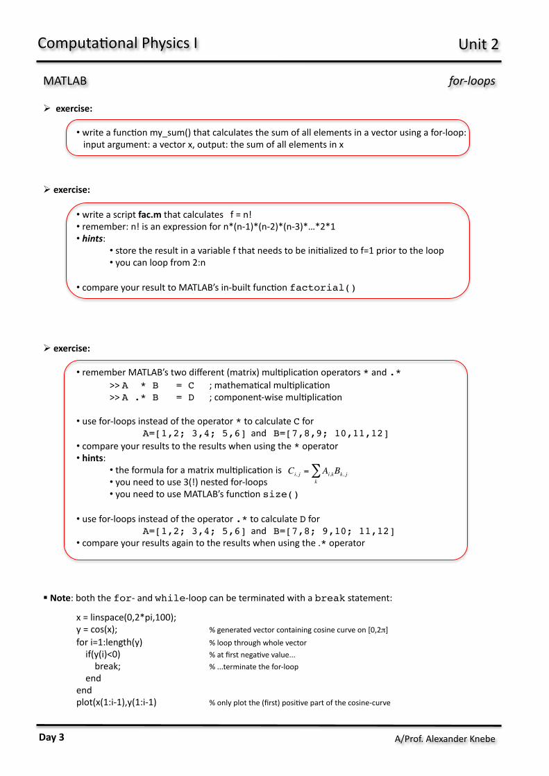
" exercise:
• write a func;on my_sum() that calculates the sum of all elements in a vector using a for-‐loop: input argument: a vector x, output: the sum of all elements in x
" exercise:
• write a script fac.m that calculates f = n! • remember: n! is an expression for n*(n-‐1)*(n-‐2)*(n-‐3)*…*2*1 • hints:
• store the result in a variable f that needs to be ini;alized to f=1 prior to the loop • you can loop from 2:n
• compare your result to MATLAB’s in-‐built func;on factorial()
" exercise:
• remember MATLAB’s two different (matrix) mul;plica;on operators * and .*>> A * B = C ; mathema;cal mul;plica;on >> A .* B = D ; component-‐wise mul;plica;on
• use for-‐loops instead of the operator * to calculate C for A=[1,2; 3,4; 5,6] and B=[7,8,9; 10,11,12]
• compare your results to the results when using the * operator • hints:
• the formula for a matrix mul;plica;on is • you need to use 3(!) nested for-‐loops • you need to use MATLAB’s func;on size()
• use for-‐loops instead of the operator .* to calculate D for A=[1,2; 3,4; 5,6] and B=[7,8; 9,10; 11,12]
• compare your results again to the results when using the .* operator
for-‐loops
Computa;onal Physics I Unit 2
€
Ci, j = Ai,kBk, jk∑
Day 3
! Note: both the for-‐ and while-‐loop can be terminated with a break statement:
x = linspace(0,2*pi,100); y = cos(x); % generated vector containing cosine curve on [0,2π] for i=1:length(y) % loop through whole vector if(y(i)<0) % at first nega;ve value... break; % ...terminate the for-‐loop end end plot(x(1:i-‐1),y(1:i-‐1) % only plot the (first) posi;ve part of the cosine-‐curve

A/Prof. Alexander Knebe
MATLAB switch statement
Computa;onal Physics I Unit 2
! in case you have mul;ple op;ons, there exist the switch statement
switch expression: case A,
command, command, ...
case B, command, command, ...
... ...
otherwise, command, command, ...
end
" exercise:
• write a script that uses input() to take a number between 1 and 7 from the user • use the switch statement to display (using disp())
• ‘Monday’ if that number was 1, • ‘Tuesday’ if that number was 2, • ‘Wednesday’ if that number was 3, • etc.
• use the ‘otherwise’ statement to display an error message in case the number is not in the allowed range
! the switch expression can also be a string!
" exercise:
• write a script that uses input() to take both a number and a string from the user: • x = variable for the number • unit = string variable for either ‘meter’ or ‘inch’
• use a switch for unit to decide whether to convert x to meter or inch • case ‘inch’, y = x/39.3701 (converion to meter) • case ‘meter’, y = x*39.3701 (conversion to inch)
• use the ‘otherwise’ statement to display an error message in case unit does neither contain ‘meter’ nor ‘inch’
Day 3
A/Prof. Alexander Knebe
MATLAB applica0on – gravity
Computa;onal Physics I Unit 2
Day 4
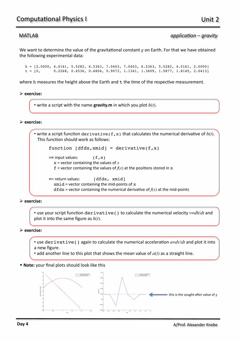
We want to determine the value of the gravita;onal constant g on Earth. For that we have obtained the following experimental data:
h = [2.0000, 4.0161, 5.5282, 6.5363, 7.0403, 7.0403, 6.5363, 5.5282, 4.0161, 2.0000]t = [0, 0.2268, 0.4536, 0.6804, 0.9073, 1.1341, 1.3609, 1.5877, 1.8145, 2.0413]
where h measures the height above the Earth and t the ;me of the respec;ve measurement. " exercise:
• write a script with the name gravity.m in which you plot h(t).
" exercise:
• write a script func;on derivative(f,x) that calculates the numerical deriva;ve of h(t). This func;on should work as follows:
function [dfdx,xmid] = derivative(f,x)
⟹ input values: (f,x) x = vector containing the values of x f = vector containing the values of f(x) at the posi;ons stored in x
⟸ return values: [dfdx, xmid] xmid = vector containing the mid-‐points of x dfdx = vector containing the numerical deriva;ve of f(x) at the mid-‐points
" exercise:
• use your script func;on derivative() to calculate the numerical velocity v=dh/dt and plot it into the same figure as h(t).
" exercise:
• use derivative() again to calculate the numerical accelera;on a=dv/dt and plot it into a new figure. • add another line to this plot that shows the mean value of a(t) as a straight line.
! Note: your final plots should look like this
t [s]0 0.5 1 1.5 2 2.5
h(t)
[m] &
v(t)
[m/s
]
-10
-8
-6
-4
-2
0
2
4
6
8
10experimental positionnumerical velocity
t [s]0.2 0.4 0.6 0.8 1 1.2 1.4 1.6 1.8 2
a [m
/s2 ]
-9.804
-9.802
-9.8
-9.798
-9.796
-9.794
-9.792
-9.79numerical accelerationmean acceleration
this is the sought-‐arer value of g
A/Prof. Alexander Knebe
MATLAB
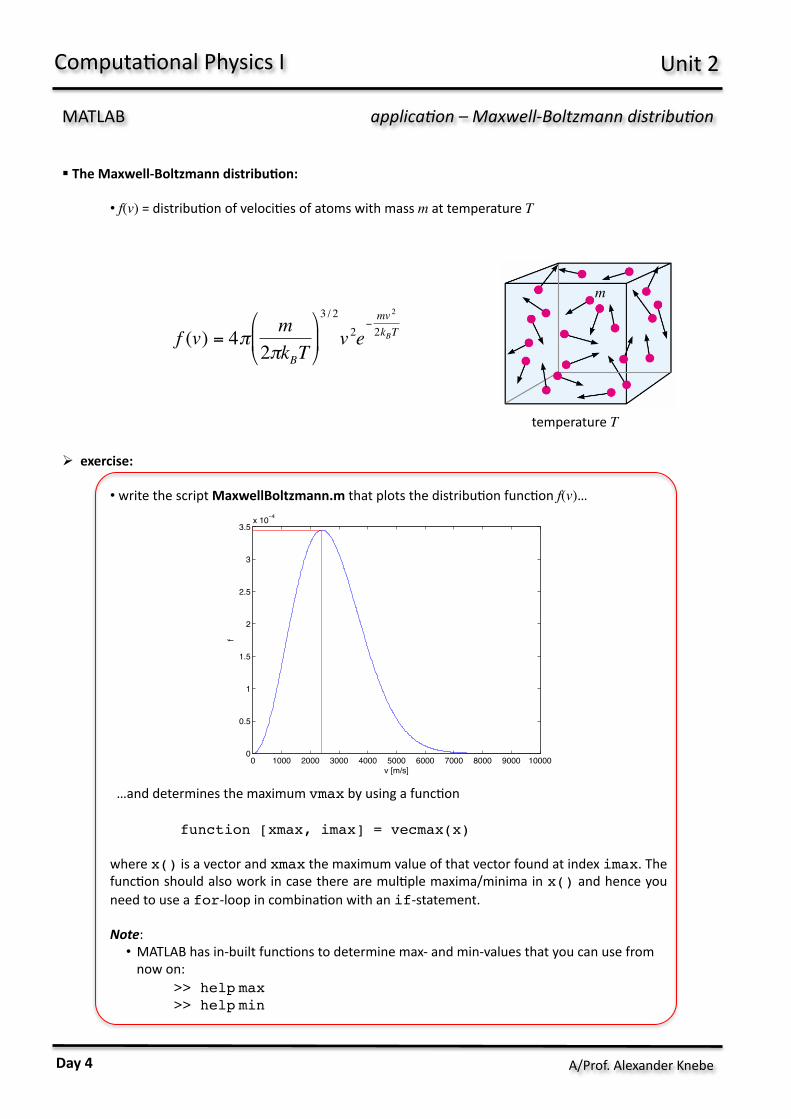
! The Maxwell-‐Boltzmann distribu<on:
• f(v) = distribu;on of veloci;es of atoms with mass m at temperature T
applica0on – Maxwell-‐Boltzmann distribu0on
Computa;onal Physics I Unit 2
€
f (v) = 4π m2πkBT#
$ %
&
' (
3 / 2
v 2e−mv 2
2kBT
temperature T
m
Day 4
0 1000 2000 3000 4000 5000 6000 7000 8000 9000 100000
0.5
1
1.5
2
2.5
3
3.5x 10⁻⁴
v [m/s]
f
" exercise:
• write the script MaxwellBoltzmann.m that plots the distribu;on func;on f(v)…
…and determines the maximum vmax by using a func;on function [xmax, imax] = vecmax(x)
where x() is a vector and xmax the maximum value of that vector found at index imax. The func;on should also work in case there are mul;ple maxima/minima in x() and hence you need to use a for-‐loop in combina;on with an if-‐statement.
Note: • MATLAB has in-‐built func;ons to determine max-‐ and min-‐values that you can use from now on:
>> help max >> help min
A/Prof. Alexander Knebe
MATLAB
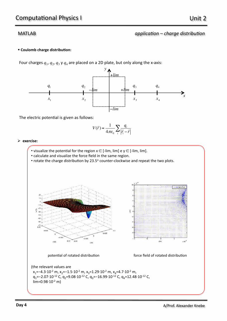
! Coulomb charge distribu<on:
applica0on – charge distribu0on
Computa;onal Physics I Unit 2
Day 4
Four charges q1, q2, q3 y q4 are placed on a 2D plate, but only along the x-‐axis: The electric poten;al is given as follows:
€
q1
€
q2
€
q3
€
q4€
+lim
€
−lim€
+lim
€
−lim
€
x€
y
V (!r ) = 14πε0
qi!ri −!ri
∑
€
x1
€
x2
€
x3
€
x4
" exercise:
• visualize the poten;al for the region x ∈ [-‐lim, lim] e y ∈ [-‐lim, lim]. • calculate and visualize the force field in the same region. • rotate the charge distribu;on by 23.5o counter-‐clockwise and repeat the two plots.
(the relevant values are x1=−4.3·∙10-‐2 m, x2=−1.5·∙10-‐2 m, x3=1.29·∙10-‐2 m, x4=4.7·∙10-‐2 m, q1=−2.07·∙10-‐12 C, q2=9.08·∙10-‐12 C, q3=−16.99·∙10-‐12 C, q4=12.48·∙10-‐12 C, lim=0.98·∙10-‐2 m)
poten;al of rotated distribu;on force field of rotated distribu;on
A/Prof. Alexander Knebe
0.5 1 1.5 2 2.5 3 3.5
1
1.5
2
2.5
3
MATLAB applica0on – Lissajous curves
Computa;onal Physics I Unit 2
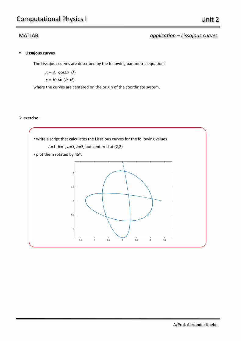
! Lissajous curves
The Lissajous curves are described by the following parametric equa;ons
where the curves are centered on the origin of the coordinate system.
" exercise:
• write a script that calculates the Lissajous curves for the following values A=1, B=1, a=5, b=3, but centered at (2,2)
• plot them rotated by 45o:
x = A ⋅cos(a ⋅θ )y = B ⋅sin(b ⋅θ )
A/Prof. Alexander Knebe
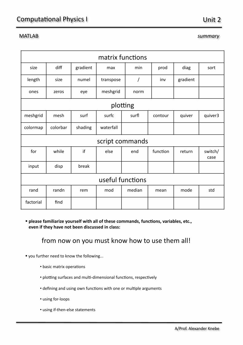
MATLAB summary
matrix func;ons size diff gradient max min prod diag sort
length size numel transpose / inv gradient
ones zeros eye meshgrid norm
plo7ng meshgrid mesh surf surfc surfl contour quiver quiver3
colormap colorbar shading waterfall
script commands for while if else end func;on return switch/
case
input disp break
useful func;ons rand randn rem mod median mean mode std
factorial find
! you further need to know the following...
• basic matrix opera;ons
• plo7ng surfaces and mul;-‐dimensional func;ons, respec;vely
• defining and using own func;ons with one or mul;ple arguments
• using for-‐loops
• using if-‐then-‐else statements
Computa;onal Physics I Unit 2
! please familiarize yourself with all of these commands, func<ons, variables, etc., even if they have not been discussed in class:
from now on you must know how to use them all!