(12.14)

UNIT-V

TRAFFIC ANALYSIS

Except for station sets and their associated loops, a telephone network is

composed of a variety of common equipment such as digit receivers, call processors,

interstage switching links, and interoffice trunks. The amount of common equipment

designed into a network is determined under an assumption that not all users of the

network need service at one time. The exact amount of common equipment required is

unpredictable because of the random nature of the service requests. Networks conceivably

could be designed with enough common equipment to instantly service all requests except

for occurrences of very rare or unanticipated peaks. However, this solution is

uneconomical because much of the common equipment is unused during normal network

loads. The basic goal of traffic analysis is to provide a method for determining the cost-

effectiveness of various sizes and configurations of networks.

Traffic in a communications network refers to the aggregate of all user requests

being serviced by the network. As far as the network is concerned, the service requests

arrive randomly and usually require unpredictable service times. The first step of traffic

analysis is the characterization of traffic arrivals and service times in a probabilistic

framework. Then the effectiveness of a network can be evaluated in terms of how much

traffic it carries under normal or average loads and how often the traffic volume exceeds

the capacity of the network.

The techniques of traffic analysis can be divided into two general categories:

loss systems and delay systems. The appropriate analysis category for a particular system

depends on the system’s treatment of overload traffic. In a loss system overload traffic is

rejected without being serviced. In a delay system overload traffic is held in a queue until

the facilities become available to service it. Conventional circuit switching operates as a

loss system since excess traffic is blocked and not serviced without a retry on the part of

the user. In some instances “lost” calls actually represent a loss of revenue to the carriers

by virtue of their not being completed.

Store-and-forward message or packet switching obviously possesses the basic

characteristics of a delay system. Sometimes, however, a packet-switching operation can

also contain certain aspects of a loss system. Limited queue sizes and virtual circuits both

imply loss operations during traffic overloads. Circuit-switching networks also incorporate

certain operations of a delay nature in addition to the loss operation of the circuits

themselves. For example, access to a digit receiver, an operator, or a call processor is

normally controlled by a queuing process.

The basic measure of performance for a loss system is the probability of

rejection (blocking probability). A delay system, on the other hand, is measured in terms

of service delays. Sometimes the average delay is desired, while at other times the prob-

ability of the delay exceeding some specified value is of more interest.

TRAFFIC CHARACTERIZATION

Because of the random nature of network traffic, the following analyses involve

certain fundamentals of probability theory and stochastic processes. In this treatment only

the most basic assumptions and results of traffic analysis are presented. The intent is to

provide an indication of how to apply results of traffic analysis, not to delve deeply into

analytical formulations. However, a few basic derivations are presented to acquaint the

user with assumptions in the models so they can be appropriately applied.

In the realm of applied mathematics, where these subjects are treated more for-

mally, blocking probability analyses are referred to as congestion theory and delay

analyses are referred to as queuing theoiy. These topics are also commonly referred to as

traffic flow analysis. In a circuit-switched network, the “flow” of messages is not so much

of a concern as are the holding times of common equipment. A circuit- switched network

establishes an end-to-end circuit involving various network facilities (transmission links

and switching stages) that are held for the duration of a call. From a network point of

view, it is the holding of these resources that is important, not the flow of information

within individual circuits. '

On the other hand, message-switching and packet-switching networks are

directly concerned with the actual flow of information, since in these systems traffic on

the transmission links is directly related to the activity of the sources.

Circuit switching does involve certain aspects of traffic flow in the process of

setting up a connection. Connect requests flow from the sources to the destinations

acquiring, holding, and releasing certain resources in the process. As was discussed,

controlling the flow of connect requests during network overloads is a vital function of

network management.

The unpredictable nature of communications traffic arises as a result of two

underlying random processes: call arrivals and holding times. An arrival from any

particular user is generally assumed to occur purely by chance and be totally independent

of arrivals from other users. Thus the number of arrivals during any particular time

interval is indeterminate. In most cases holding times are also distributed randomly. In

some applications this element of randomness can be removed by assuming constant

holding times (e.g., fixed-length packets). In either case the traffic load presented to a net-

work is fundamentally dependent on both the frequency of arrivals and the average

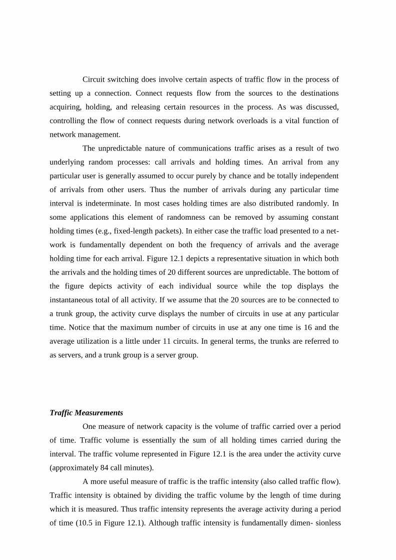
holding time for each arrival. Figure 12.1 depicts a representative situation in which both

the arrivals and the holding times of 20 different sources are unpredictable. The bottom of

the figure depicts activity of each individual source while the top displays the

instantaneous total of all activity. If we assume that the 20 sources are to be connected to

a trunk group, the activity curve displays the number of circuits in use at any particular

time. Notice that the maximum number of circuits in use at any one time is 16 and the

average utilization is a little under 11 circuits. In general terms, the trunks are referred to

as servers, and a trunk group is a server group.

Traffic Measurements

One measure of network capacity is the volume of traffic carried over a period

of time. Traffic volume is essentially the sum of all holding times carried during the

interval. The traffic volume represented in Figure 12.1 is the area under the activity curve

(approximately 84 call minutes).

A more useful measure of traffic is the traffic intensity (also called traffic flow).

Traffic intensity is obtained by dividing the traffic volume by the length of time during

which it is measured. Thus traffic intensity represents the average activity during a period

of time (10.5 in Figure 12.1). Although traffic intensity is fundamentally dimen- sionless

(time divided by time), it is usually expressed in units of erlangs, after the Danish pioneer

traffic theorist A. K. Erlang, or in terms of hundred (century) call seconds per hour (CCS).

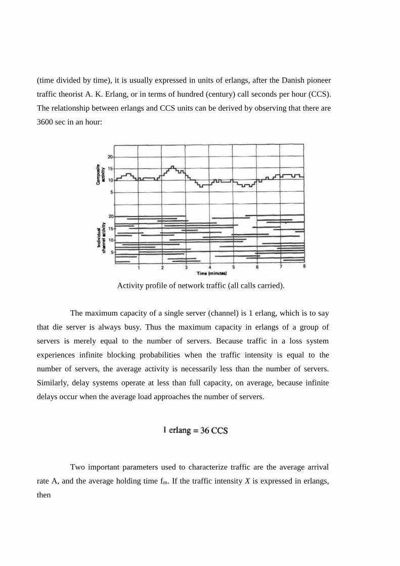
The relationship between erlangs and CCS units can be derived by observing that there are

3600 sec in an hour:

The maximum capacity of a single server (channel) is 1 erlang, which is to say

that die server is always busy. Thus the maximum capacity in erlangs of a group of

servers is merely equal to the number of servers. Because traffic in a loss system

experiences infinite blocking probabilities when the traffic intensity is equal to the

number of servers, the average activity is necessarily less than the number of servers.

Similarly, delay systems operate at less than full capacity, on average, because infinite

delays occur when the average load approaches the number of servers.

Two important parameters used to characterize traffic are the average arrival

rate A, and the average holding time fm. If the traffic intensity X is expressed in erlangs,

then

Activity profile of network traffic (all calls carried).

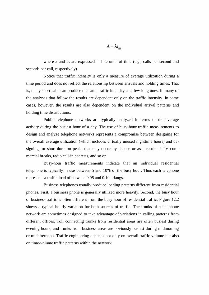
where k and tm are expressed in like units of time (e.g., calls per second and

seconds per call, respectively).

Notice that traffic intensity is only a measure of average utilization during a

time period and does not reflect the relationship between arrivals and holding times. That

is, many short calls can produce the same traffic intensity as a few long ones. In many of

the analyses that follow the results are dependent only on the traffic intensity. In some

cases, however, the results are also dependent on the individual arrival patterns and

holding time distributions.

Public telephone networks are typically analyzed in terms of the average

activity during the busiest hour of a day. The use of busy-hour traffic measurements to

design and analyze telephone networks represents a compromise between designing for

the overall average utilization (which includes virtually unused nighttime hours) and de-

signing for short-duration peaks that may occur by chance or as a result of TV com-

mercial breaks, radio call-in contests, and so on.

Busy-hour traffic measurements indicate that an individual residential

telephone is typically in use between 5 and 10% of the busy hour. Thus each telephone

represents a traffic load of between 0.05 and 0.10 erlangs.

Business telephones usually produce loading patterns different from residential

phones. First, a business phone is generally utilized more heavily. Second, the busy hour

of business traffic is often different from the busy hour of residential traffic. Figure 12.2

shows a typical hourly variation for both sources of traffic. The trunks of a telephone

network are sometimes designed to take advantage of variations in calling patterns from

different offices. Toll connecting trunks from residential areas are often busiest during

evening hours, and trunks from business areas are obviously busiest during midmoming

or midafternoon. Traffic engineering depends not only on overall traffic volume but also

on time-volume traffic patterns within the network.

Traffic volume dependence on time of day.

A certain amount of care must be exercised when determining the total traffic

load of a system from the loading of individual lines or trunks. For example, since two

phones are involved in each connection, the total load on a switching system is exactly

one-half the total of all traffic on the lines connected to the switch. In addition, it may be

important to include certain setup and release times into the average holding times of some

common equipment. A 10-sec setup time is not particularly significant for a 4-min voice

call but can actually dominate the holding time of equipment used for short data messages.

Common equipment setup times also become more significant in the presence of voice

traffic overloads. A greater percentage of the overall load is represented by call attempts

since they increase at a faster rate than completions.

An important distinction to be made when discussing traffic in a

communications network is the difference between the offered traffic and the carried

traffic. The offered traffic is the total traffic that would be carried by a network capable of

servicing all requests as they arise. Since economics generally precludes designing a

network to immediately cany the maximum offered traffic, a small percentage of offered

traffic typically experiences network blocking or delay. When the blocked calls are

rejected by the network, the mode of operation is referred to as blocked calls cleared or

lost calls cleared. In essence, blocked calls are assumed to disappear and never return.

This assumption is most appropriate for trunk groups with alternate routes. In this case a

blocked call is normally serviced by another trunk group and does not, in fact, return.

The carried traffic of a loss system is always less than the offered traffic. A

delay system, on the other hand, does not reject blocked calls but holds them until the nec-

essary facilities are available. With the assumption that the long-term average of offered

traffic is less than the capacity of the network, a delay system carries all offered traffic. If

the number of requests that can be waiting for service is limited, however, a delay system

also takes on properties of a loss system. For example, if the queue for holding blocked

arrivals is finite, requests arriving when the queue is full are cleared.

Arrival Distributions

The most fundamental assumption of classical traffic analysis is that call arrivals

are independent. That is, an arrival from one source is unrelated to an arrival from any

other source. Even though this assumption may be invalid in some instances, it has

general usefulness for most applications. In those cases where call arrivals tend to be

correlated, useful results can still be obtained by modifying a random arrival analysis. In

this manner the random arrival assumption provides a mathematical formulation that can

be adjusted to produce approximate solutions to problems that are otherwise

mathematically intractable.

Negative Exponential Interarrival Times

Designate the average call arrival rate from a large group of independent

sources (subscriber lines) as X. Use the following assumptions:

1. Only one arrival can occur in any sufficiently small interval.

2. The probability of an arrival in any sufficiently small interval is directly

proportional to the length of the interval. (The probability of an arrival is X At,

where At is the interval length.) ’

3. The probability of an arrival in any particular interval is independent of

what has occurred in other intervals.

It is straightforward [1] to show that the probability distribution of interamval

times is

Equation defines the probability that no arrivals occur in a randomly selected interval t.

This is identical to the probability that t seconds elapse from one arrival to the next.

A more subtle implication of the independent arrival assumption involves the

number of sources, not just their calling patterns. When the probability of an arrival in any

small time interval is independent of other arrivals, it implies that the number of sources

available to generate requests is constant. If a number of arrivals occur immediately before

any subinterval in question, some of the sources become busy and cannot generate

requests. The effect of busy sources is to reduce the average arrival rate. Thus the

interarrival times are always somewhat larger than what Equation predicts them to be. The

only time the arrival rate is truly independent of source activity is when an infinite number

of sources exist.

If the number of sources is large and their average activity is relatively low,

busy sources do not appreciably reduce the arrival rate. For example, consider an end

office that services 10,000 subscribers with 0.1 erlang of activity each. Normally, there are

1000 active links and 9000 subscribers available to generate new arrivals. If the number of

active subscribers increases by an unlikely 50% to 1500 active lines, the number of idle

subscribers reduces to 8500, a change of only 5.6%. Thus the arrival rate is relatively

constant over a wide range of source activity. Whenever the arrival rate is fairly constant

for the entire range of normal source activity, an infinite source assumption is justified.

It is pointed out that Lee graph analyses overestimate the blocking probability

because, if some number of interstage links in a group are known to be busy, the

remaining links in the group are less likely to be busy. A Jacobaeus analysis produces a

more rigorous and accurate solution to the blocking probability, particularly when space

expansion is used. Accurate analyses of interarrival times for finite sources are also

possible. These are included in the blocking analyses to follow.

Poisson Arrival Distribution

Equation merely provides a means of determining the distribution of interarrival

times. It does not, by itself, provide the generally more desirable information of how many

is

arrivals can be expected to occur in some arbitrary time interval. Using the same

assumptions presented, however, the probability of j arrivals in an interval t can be de-

termined as

Equation 12.3 is the well-known Poisson probability law. Notice that when j =

0, the probability of no arrivals in an interval t is P0(t), as obtained in Equation 12.2. '

Again, Equation 12.3 assumes arrivals are independent and occur at a given average rate

irrespective of the number of arrivals occurring just prior to an interval in question. Thus

the Poisson probability distribution should only be used for arrivals from a large number

of independent sources.

Equation defines the probability of experiencing exactly j arrivals in t seconds.

Usually there is more interest in determining the probability of j or more arrivals in t

seconds:

Holding Time Distributions

The second factor of traffic intensity as specified in Equation 12.1 is the average

holding time tm. In some cases the average of the holding times is all that needs to be

known about holding times to determine blocking probabilities in a loss system or delays

in a delay system. In other cases it is necessary to know the probability distribution of the

holding times to obtain the desired results. This section describes the two most commonly

assumed holding time distributions: constant holding times and exponential holding times.

Constant Holding Times

Although constant holding times cannot be assumed for conventional voice

conversations, it is a reasonable assumption for such activities as per-call call processing

requirements, interoffice address signaling, operator assistance, and recorded message

playback. Furthermore, constant holding times are obviously valid for transmission times

in fixed-length packet networks.

When constant holding time messages are in effect, it is straightforward to use

Equation 12.3 to determine the probability distribution of active channels. Assume, for the

time being, that all requests are serviced. Then the probability of j channels being busy at

any particular time is merely the probability that j arrivals occurred in the time interval of

length tm immediately preceding the instant in question. Since the average number of

active circuits over all time is the traffic intensity A = Xtm, the probability ofy circuits

being busy is dependent only on the traffic intensity:

Exponential Holding Times

The most commonly assumed holding time distribution for conventional

telephone conversations is the exponential holding time distribution:

where rm is the average holding time. Equation 12.6 specifies the probability

that a holding time exceeds the value t. This relationship can be derived from a few

simple assumptions concerning the nature of the call termination process. Its basic

justification, however, lies in the fact that observations of actual voice conversations

exhibit a remarkably close correspondence to an exponential distribution.

The exponential distribution possesses the curious property that the probability

of a termination is independent of how long a call has been in progress. That is, no matter

how long a call has been in existence, the probability of it lasting another t seconds is

defined by Equation 12.6. In this sense exponential holding times represent the most

random process possible. Not even knowledge of how long a call has been in progress

provides any information as to when the call will terminate.

Combining a Poisson arrival process with an exponential holding time process

to obtain the probability distribution of active circuits is more complicated than it was for

constant holding times because calls can last indefinitely. The final result, however,

proves to be dependent on only the average holding time. Thus Equation 12.5 is valid for

exponential holding times as well as for constant holding times (or any holding time

distribution). Equation 12.5 is therefore repeated for emphasis: The probability of j

circuits being busy at any particular instant, assuming a Poisson arrival process and that

all requests are serviced immediately, is

where A is the traffic intensity in erlangs. This result is true for any distribution

of holding times.

LOSS SYSTEMS

The basic reason for the discrepancy is indicated in Figure 12.3, which depicts

the same traffic pattern arising from 20 sources as is shown previously in Figure 12.1.

Figure 12.3, however, assumes that only 13 circuits are available to carry the traffic. Thus

the three arrivals at t — 2.2, 2.3, and 2.4 min are blocked and assumed to have left the

system. The total amount of traffic volume lost is indicated by the shaded area, which is

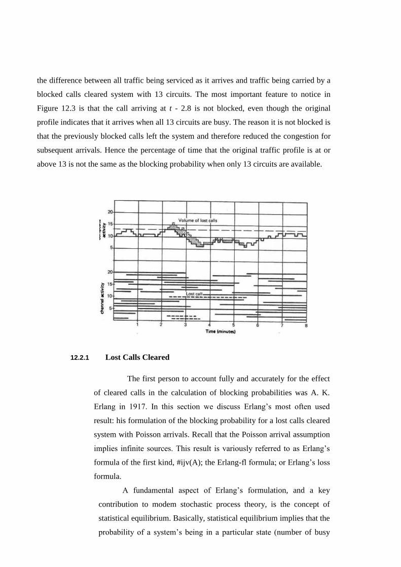
the difference between all traffic being serviced as it arrives and traffic being carried by a

blocked calls cleared system with 13 circuits. The most important feature to notice in

Figure 12.3 is that the call arriving at t - 2.8 is not blocked, even though the original

profile indicates that it arrives when all 13 circuits are busy. The reason it is not blocked is

that the previously blocked calls left the system and therefore reduced the congestion for

subsequent arrivals. Hence the percentage of time that the original traffic profile is at or

above 13 is not the same as the blocking probability when only 13 circuits are available.

12.2.1 Lost Calls Cleared

The first person to account fully and accurately for the effect

of cleared calls in the calculation of blocking probabilities was A. K.

Erlang in 1917. In this section we discuss Erlang’s most often used

result: his formulation of the blocking probability for a lost calls cleared

system with Poisson arrivals. Recall that the Poisson arrival assumption

implies infinite sources. This result is variously referred to as Erlang’s

formula of the first kind, #ijv(A); the Erlang-fl formula; or Erlang’s loss

formula.

A fundamental aspect of Erlang’s formulation, and a key

contribution to modem stochastic process theory, is the concept of

statistical equilibrium. Basically, statistical equilibrium implies that the

probability of a system’s being in a particular state (number of busy

circuits in a trunk group) is independent of the time at which the

system is examined. For a system to be in statistical equilibrium, a

long time must pass (several average holding times) from when the

system is in a known state until it is again examined. For example,

when a trunk group first begins to accept traffic, it has no busy circuits.

For a short time thereafter, the system is most likely to have only a few

busy circuits. As time passes, however, the system reaches

equilibrium. At this point the most likely state of the system is to have

A = Xtm busy circuits.

When in equilibrium, a system is as likely to have an arrival as

it is to have a termination. If the number of active circuits happens to

increase above the average A, departures become more likely than

arrivals. Similarly, if the number of active circuits happens to drop

below A, an arrival is more likely than a departure. Thus if a system is

perturbed by chance from its average state, it tends to return.

Although Erlang’s elegant formulation is not

particularly complicated, it is not presented here because we are mostly

interested in application of the results. The interested reader is invited

to see reference [2] or [3] for a derivation of the result:

Equation specifies the probability of blocking for a system with random arrivals from an

infinite source and arbitrary holding time distributions. The blocking probability of

Equation 12.8 is plotted in Figure 12.4 as a function of offered traffic intensity for various

numbers of channels. An often more useful presentation of Erlang’ s results is provided in

Figure 12.5, which presents the output channel utilization for various blocking probabilities

and numbers of servers. The output utilization p represents the traffic carried by each

circuit:

Blocking probability of lost calls cleared system.

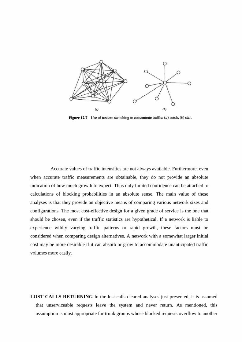
(1The greater circuit efficiency obtained by combining traffic into large groups

is often referred to as the advantage of large group sizes. This efficiency of circuit utili-

zation is the basic motivation for hierarchical switching structures. Instead of intercon-

necting a large number of nodes with rather small trunk groups between each pair, it is

more economical to combine all traffic from individual nodes into one large trunk group

and route the traffic through a tandem switching node. Figure 12.7 contrasts a mesh versus

a star network with a centralized switching node at the center. Obviously, the cost of the

tandem switch becomes justified when the savings in total circuit miles is large enough

Accurate values of traffic intensities are not always available. Furthermore, even

when accurate traffic measurements are obtainable, they do not provide an absolute

indication of how much growth to expect. Thus only limited confidence can be attached to

calculations of blocking probabilities in an absolute sense. The main value of these

analyses is that they provide an objective means of comparing various network sizes and

configurations. The most cost-effective design for a given grade of service is the one that

should be chosen, even if the traffic statistics are hypothetical. If a network is liable to

experience wildly varying traffic patterns or rapid growth, these factors must be

considered when comparing design alternatives. A network with a somewhat larger initial

cost may be more desirable if it can absorb or grow to accommodate unanticipated traffic

volumes more easily.

LOST CALLS RETURNING In the lost calls cleared analyses just presented, it is assumed

that unserviceable requests leave the system and never return. As mentioned, this

assumption is most appropriate for trunk groups whose blocked requests overflow to another

route and are usually serviced elsewhere. However, lost calls cleared analyses are also used

in instances where blocked calls do not get serviced elsewhere. In many of these cases,

blocked calls tend to return to the system in the form of retries. Some examples are

subscriber concentrator systems, corporate tie lines and PBX trunks, calls to busy telephone

numbers, and access to WATS lines (if DDD alternatives are not used). This section derives

blocking probability relationships for lost calls cleared systems with random retries.The

following analysis involves three fundamental assumptions regarding the nature of the

returning calls:All blocked calls return to the system and eventually get serviced, even if

multiple retries are required.The elapsed times between call blocking occurrences and the

generation of retries are random and statistically independent of each other. (This

assumption allows the analysis to avoid complications arising when retries are correlated to

each other and tend to cause recurring traffic peaks at a particular waiting time interval.) The

typical waiting time before retries occur is somewhat longer than the average holding time

of a connection. This assumption essentially states that the system is allowed to reach

statistical equilibrium before a retry occurs. Obviously, if retries occur too soon, they are

very likely to encounter congestion since the system has not had a chance to “relax.” In the

limit, if all retries are immediate and continuous, the network operation becomes similar to a

delay system. In this case, however, the system does not queue requests—the sources do so

by continually “redialing.” When considered in their entirety, these assumptions characterize

retries as being statistically indistinguishable from first-attempt traffic.* Hence blocked calls

merely add to the first-attempt call arrival rate. Consider a system with a first-attempt call

arrival rate of X. If a percentage B of the calls is blocked, B times X retries will occur in the

future. Of these retries, however, a percentage B will be blocked again. Continuing in this

manner, the total arrival rate X' after the system has reached statistical equilibrium can be

determined as the infinite series

where B is the blocking probability from a lost calls cleared analysis with traffic

cleared analysis of Equation 12.8. First, determine an estimate of B using X and

then calculate X'. Next, use V to obtain a new value of B and an updated value of V. Con-

tinue in this manner until values of X and B are obtained.

When measurements are made to determine the blocking probability of an

outgoing trunk group, the measurements cannot distinguish between first-attempt calls

(demand traffic) and retries. Thus if a significant number of retries are contained in the

measurements, this fact should be incorporated into an analysis of how many circuits must

be added to reduce the blocking of an overloaded trunk group. The apparent offered load

will decrease as the number of servers increases because the number of re- tries decreases.

Thus fewer additional circuits are needed than if no retries are contained in the

measurements.

\

Lost Calls Held

In a lost calls held system, blocked calls are held by the system and serviced

when the necessary facilities become available. Lost calls held systems are distinctly

different from the delay systems discussed later in one important respect: The total elapsed

time of a call in the system, including waiting time and service time, is independent of the

waiting time. In essence, each arrival requires service for a continuous period of time and

terminates its request independently of its being serviced or not. Figure 12.9 demonstrates

the basic operation of a lost calls held system. Notice that most blocked calls eventually

get some service, but only for a portion of the time that the respective sources are busy.

Although a switched telephone network does not operate in a lost calls held

manner, some systems do. Lost calls held systems generally arise in real-time applications

in which the sources are continuously in need of service, whether or not the facilities are

available. When operating under conditions of heavy traffic, a lost calls held system

typically provides service for only a portion of the time a particular source is active.

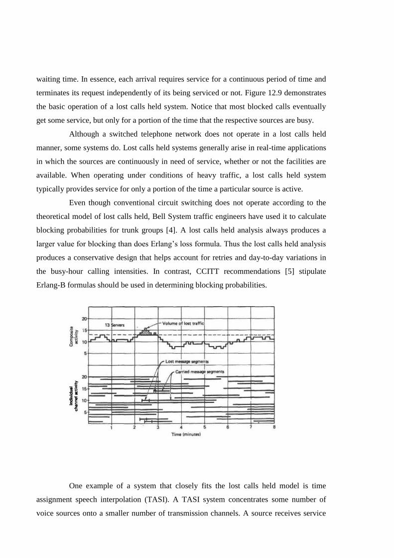
Even though conventional circuit switching does not operate according to the

theoretical model of lost calls held, Bell System traffic engineers have used it to calculate

blocking probabilities for trunk groups [4]. A lost calls held analysis always produces a

larger value for blocking than does Erlang’s loss formula. Thus the lost calls held analysis

produces a conservative design that helps account for retries and day-to-day variations in

the busy-hour calling intensities. In contrast, CCITT recommendations [5] stipulate

Erlang-B formulas should be used in determining blocking probabilities.

One example of a system that closely fits the lost calls held model is time

assignment speech interpolation (TASI). A TASI system concentrates some number of

voice sources onto a smaller number of transmission channels. A source receives service

(is connected to a channel) only when it is active. If a source becomes active when all

channels are busy, it is blocked and speech clipping occurs. Each speech segment starts

and stops independently of whether it is serviced or not. TASI systems were originally

used on analog long-distance transmission links such as undersea cables. More modem

counterparts of TASI are referred to as digital circuit multiplication (DCM) systems. In

contrast to the original TASI systems, DCM systems can delay speech for a small amount

of time, when necessary, to minimize the clipping. In this case, a lost calls held analysis is

not rigorously justified because the total time a speech segment is “in the system”

increases as the delay for service increases. However, if the average delay is a small

percentage of the holding time, or if the coding rate of delayed speech is reduced to allow

the transmission channel time to “catch up,” a lost calls held analysis is still justified.

Recall that controlling the coding rate is one technique of traffic shaping used for

transporting voice in an ATM network.

Lost calls held systems are easily analyzed to determine the probability of the

total number of calls in the system at any one time. Since the duration of a source’s

activity is independent of whether it is being serviced, the number in the system at any

timp is identical to the number of active sources in a system capable of carrying all traffic

as it arises. Thus the distribution of the number in the system is the Poisson distribution

provided earlier in Equation 12.3. The probability that i sources requesting service are

being blocked is simply the probability that i + N sources are active when N i s the number

of servers. Recall that the Poisson distribution essentially determines the desired

probability as the probability that i + N arrivals occurred in the preceding fra seconds. The

distribution is dependent only on the product of the average arrival rate X and the average

holding time tm.

Example 12.9 demonstrates that TASI systems are much more effective for

large group sizes than for small ones. The 36% clipping factor occurring with 5 channels

produces unacceptable voice quality. On the other hand, the 4% clipping probability for 50

channels can be tolerated when the line costs are high enough.

In reality, the values for blocking probabilities obtained in Example 12.9 are

overly pessimistic because an infinite source assumption was used. The summations did

not include the case of all sources being active because there needs to be at least one idle

source to create an arrival during the time congestion. A more accurate solution to this

problem is obtained in a later section using a finite source analysis.

Lost Calls Cleared—Finite Sources

As mentioned previously, a fundamental assumption in the derivation of the

Poisson arrival distribution, and consequently Erlang’s loss formula, is that call arrivals

occur independently of the number of active callers. Obviously, this assumption can be

justified only when the number of sources is much larger than the number of servers. This

section presents some fundamental relationships for determining blocking probabilities of

lost calls cleared systems when the number of sources is not much larger than the number

of servers. The blocking probabilities in these cases are always less than those for infinite

source systems since the arrival rate decreases as the number of busy sources increases.

When considering finite source systems, traffic theorists introduce another

parameter of interest called time congestion. Time congestion is the percentage of time

that all servers in a group are busy. It is identical to the probability that all servers are busy

at randomly selected times. However, time congestion is not necessarily identical to

blocking probability (which is sometimes referred to as call congestion). Time congestion

merely specifies the probability that all servers are busy. Before blocking can occur, there

must be an arrival.

In an infinite source system, time congestion and call congestion are identical

because the percentage of arrivals encountering all servers busy is exactly equal to the

time congestion. (The fact that all servers are busy has no bearing on whether or not an

arrival occurs.) In a finite source system, however, the percentage of arrivals encountering

congestion is smaller because fewer arrivals occur during periods when all servers are

busy. Thus in a finite source system, call congestion (blocking probability) is always less

than the time congestion. As an extreme example, consider equal numbers of sources and

servers. The time congestion is the probability that all servers are busy. The blocking

probability is obviously zero.

The same basic techniques introduced by Erlang when he determined the loss

formula for infinite sources can be used to derive loss formulas for finite sources [3], Us-

ing these techniques, we find the probability of n servers being busy in a system

with M sources and N servers is

where V is the calling rate per idle source and tm is the average holding time. Equation is

known as the truncated Bemoullian distribution and also as the Engset distribution.

Setting n = Nin Equation 12.11 produces an expression for the time congestion:

Using the fact that the arrival rate when N servers are busy is (M - N)/M times

the arrival rate when no servers are busy, we can determine the blocking probability for

lost calls cleared with a finite source as follows:

which is identical to PN (the time congestion) for M - 1 sources.

Equations are easily evaluated in terms of the parameters A,' and tm. However,

X' and tm do not, by themselves, specify the average activity of a source. In a lost calls

cleared system with finite sources the effective offered load decreases as the blocking

probability increases because blocked calls leave and do not return. When a call is

blocked, the average activity of the offering source decreases, which increases the average

amount of idle time for that source. The net result is that X' decreases because the amount

of idle time increases. If the average activity of a source assuming no traffic is cleared is

designated as p = fam, the value of X'tm can be determined as where B is the blocking

probability defined by Equation 12.13.

The difficulty with using the unblocked source activity factor p to characterize a

source’s offered load is now apparent. The value of X' fm depends on B, which in turn

depends on X' tm. Thus some form of iteration is needed to determine B when the sources

are characterized by p (an easily measured parameter) instead of X’. If the total offered

load is considered to be Mp, the carried traffic is

Blocking probability of lost calls cleared with finite sources.

A table of traffic capacities for finite sources is provided in Appendix D.2,

where the offered load A = Mp is listed for various combinations of M, N, and B. Some of

the results are plotted in Figure 12.10, where they can be compared to blocking prob-

abilities of infinite source systems. As expected, infinite source analyses (Erlang-B) are

acceptable when the number of sources M is large.

sources are used, the offered load of 7.26 erlangs is higher than the 7.04 erlangs

obtainable from interpolation in Table D.2 as the maximum offered load for B = 1%.

It is worthwhile comparing the result of Example 12.10 to a result obtained

from an infinite source analysis (Erlang-fl). For a blocking probability of 1 %, Table D. 1

reveals that the maximum offered load for 12 servers is 5.88 erlangs. Thus the maximum

number of sources can be determined as 5.88/0.333 = 17.64. Hence in this case an infinite

source analysis produces a result that is conservative by 15%.

12.2.2 Lost Calls Held—Finite Sources

A lost calls held system with finite sources is analyzed in the same basic manner

as a lost calls held systems with infinite sources. At all times the number of calls “in the

system” is defined to be identical to the number of calls that would be serviced by a

strictly nonblocking server group. Thus Equation 12.11 is used to determine the prob-

ability that exactly n calls are in the system:

Because no calls are cleared, the offered load per idle source is not dependent

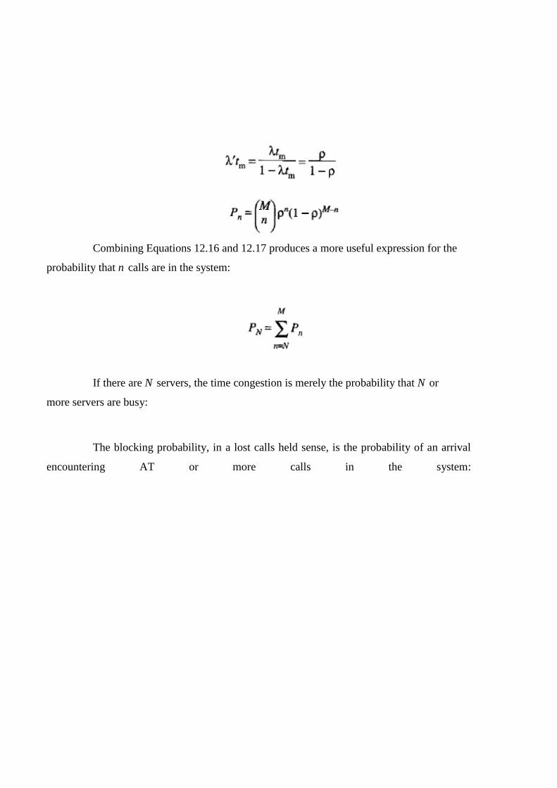
Combining Equations 12.16 and 12.17 produces a more useful expression for the

probability that n calls are in the system:

If there are N servers, the time congestion is merely the probability that N or

more servers are busy:

The blocking probability, in a lost calls held sense, is the probability of an arrival

encountering AT or more calls in the system:

where p = offered load per source M - number of sources N = number of servers

NETWORK BLOCKING PROBABILITIES

In the preceding sections basic techniques of congestion theory are presented to

determine blocking probabilities of individual trunk groups. In this section techniques of

calculating end-to-end blocking probabilities of a network with more than one routebetween

endpoints is considered. In conjunction with calculating the end-to-end blocking probabilities, it

is necessary to consider the interaction of traffic on various routes of a network. Foremost

among these considerations is the effect of overflow traffic from one route onto another. The

following sections discuss simplified analyses only. More sophisticated techniques for more

complex networks can be obtained in references [9],

End-to-End Blocking Probabilities

Generally, a connection through a large network involves a series of transmission

links, each one of which is selected from a set of alternatives. Thus an end-to-end blocking

probability analysis usually involves a composite of series and parallel probabilities. The

simplest procedure is identical to the blocking probability (matching loss) analyses for

switching networks. For example, Figure depicts a representative set of alternative connections

through a network and the resulting composite blocking probability.

The blocking probability equation in Figure 12.12 contains several simplifying as-

sumptions. First, the blocking probability (matching loss) of the switches is not included. In a

digital time division switch, matching loss can be low enough that it is easily eliminated from

the analysis. In other switches, however, the matching loss may not be insignificant. When

necessary, switch blocking is included in the analysis by considering it a source of blocking in

series with the associated trunk groups.

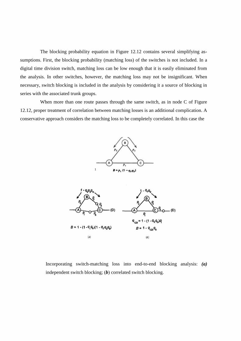
When more than one route passes through the same switch, as in node C of Figure

12.12, proper treatment of correlation between matching losses is an additional complication. A

conservative approach considers the matching loss to be completely correlated. In this case the

1

Incorporating switch-matching loss into end-to-end blocking analysis: (a)

independent switch blocking; (b) correlated switch blocking.

matching loss is in series with the common link. On the other hand, an optimistic analysis

assumes that the matching losses are independent, which implies that they are in series with the

individual links. Figure 12.13 depicts these two approaches for including the matching loss of

switch C into the end-to-end blocking probability equation of Figure 12.12. In this case, the link

from C to D is the common link.

A second simplifying assumption used in deriving the blocking probability equation

in Figure 12.12 involves assuming independence for the blocking probabilities of the trunk

groups. Thus the composite blocking of two parallel routes is merely the product of the

respective probabilities (Equation 5.4). Similarly, independence implies that the blocking

probability of two paths—in series—is 1 minus the product of the respective availabilities

(Equation 5.5). In actual practice individual blocking probabilities are never completely

independent. This is particularly true when a large amount of traffic on one route results as

overflow from another route. Whenever the first route is busy, it is likely that more than the

average amount of overflow is being diverted to the second route. Thus an alternate route is

more likely to be busy when a primary route is busy.

In a large public network, trunks to tandem or toll switches normally carry traffic to

many destinations. Thus no one direct route contributes an overwhelming amount of overflow

traffic to a particular trunk group. In this case independent blocking probabilities on alternate

routes are justified. In some instances of the public network, and often in private networks,

overflow traffic from one route dominates the traffic on tandem routes. In these cases failure to

account for the correlation in blocking probabilities can lead to overly optimistic results.

The correlations between the blocking probabilities of individual routes arise because

congestion on one route produces overflows that tend to cause congestion on other routes.

External events stimulating networkwide overloads also cause the blocking probabilities to be

correlated. Thus a third assumption in the end-to-end blocking probability equation of Figure

12.12 is that traffic throughout the network is independent. If fluctuations in the traffic volume

on individual links tend to be correlated (presumably because of external events such as

television commercials, etc.), significant degradation in overall performance results.

12.3.2 Overflow Traffic

The second source of error in Example 12.13 occurred because an Erlang-/} analysis

used the average volume of overflow traffic from the first group to determine the blocking

probability of the second trunk group. An Erlang-B analysis assumes traffic arrivals are purely

random, that is, they are modeled by a Poisson distribution. However, a Poisson arrival

distribution is an erroneous assumption for the traffic offered to the second trunk group. Even

though arrivals to the first group may be random, the overflow process tends to select groups of

these arrivals and pass them on to the second trunk group. Thus instead of being random the

arrivals to the second group occur in bursts. This overflow effect is illustrated in Figure 12.14,

which portrays a typical random arrival pattern to one trunk group and the overflow pattern to a

second group. If a significant amount of the traffic flowing onto a trunk group results as

overflow from other trunk groups, overly optimistic values of blocking probability arise when

all of the traffic is assumed to be purely random.

The most common technique of dealing with overflow traffic is to relate the overflow

traffic volume to an equivalent amount of random traffic in a blocking probability sense. For

example, if the 1.62 erlangs of overflow traffic in Example 12.12 is equated to 2.04 erlangs of

random traffic, a blocking probability of 1.3% is obtained for the second trunk group. (This is

the correct probability of blocking for the second group since both groups are busy if and only

if the second group is busy.)

This method of treating overflow traffic is referred to as the equivalent random the-

ory [12]. Tables of traffic capacity are available [13] that incorporate the overflow effects

directly into the maximum offered loads. The Neal-Wilkinson tables used by Bell System

traffic engineers comprise one such set of tables. The Neal-Wilkinson tables, however, also

incorporate the effects of day-to-day variations in the traffic load. Arrival* to first trunk group

(Forty erlangs on one day and 30 erlangs on another is not the same as 35 erlangs on

both days.) These tables are also used for trunk groups that neither generate nor receive

overflow traffic. The fact that cleared traffic does not get serviced by an alternate route implies

that retries are likely. The effect of the retries, however, is effectively incorporated into the

value of B by equivalent randomness.

DELAY SYSTEMS

The second category of teletraffic analysis concerns systems that delay

nonserviceable requests until the necessary facilities become available. These systems are

variously referred to as delay systems, waiting-call systems, and queuing systems. Call arrivals

occurring when all servers are busy are placed in a queue and held until service commences.

The queue might consist of storage facilities in a physical sense, such as blocks of memory in a

message-switching node, or the queue might consist only of a list of sources waiting for

service. In the latter case, storage of the messages is the responsibility of the sources

themselves.

Using the more general term queueing theory, we can apply the following analyses to

a wide variety of applications outside of telecommunications. Some of the more common

applications are data processing, supermarket check-out counters, aircraft landings, inventory

control, and various forms of service bureaus. These and many other applications are

considered in the field of operations research. The foundations of queuing theory, however, rest

on fundamental techniques developed by early telecommunications traffic researchers. In fact,

Erlang is credited with the first solution to the most basic type of delay system. Examples of

delay system analysis applications in telecommunications are message switching, packet

switching, statistical time division multiplexing, multipoint data communications, automatic

call distribution, digit receiver access, signaling equipment usage, and call processing.

Furthermore, many PBXs have features allowing queued access to corporate tie lines or WATS

lines. Thus some systems formerly operating as loss systems now operate as delay systems.

In general, a delay operation allows for greater utilization of servers (transmission

facilities) than does a loss system. Basically, the improved utilization is achieved because peaks

in the arrival process are “smoothed” by the queue. Even though arrivals to the system are

random, the servers see a somewhat regular arrival pattern. The effect of the queuing process on

overload traffic is illustrated in Figure 12.15. This figure displays the same traffic patterns

presented earlier in Figures 12.1,12.3, and 12.9. In this case, however, overload traffic is

delayed until call terminations produce available channels.

In most of the following analyses it is assumed that all traffic offered to the system

eventually gets serviced. One implication of this assumption is that the offered traffic intensity

A is less than the number of servers N. Even when A is less than N, there are two cases in which

the carried traffic might be less than the offered traffic. First, some sources might tire of waiting

in a long queue and abandon the request. Second, the capacity for storing requests may be

finite. Hence requests may occasionally be rejected by the system.

A second assumption in the following analyses is that infinite sources exist. In a

delay system, there may be a finite number of sources in a physical sense but an infinite number

of sources in an operational sense because each source may have an arbitrary number of

requests outstanding (e.g., a packet-switching node). There are instances in which a finite

source analysis is necessary, but not in the applications considered here.

An additional implication of servicing all offered traffic arises when infinite sources

exist. This implication is the need for infinite queuing capabilities. Even though the offered

traffic intensity is less than the number of servers, no statistical limit exists on the number of

arrivals occurring in a short period of time. Thus the queue of a purely lossless system must be

arbitrarily long. In a practical sense, only finite queues can be realized, so either a statistical

chance of blocking is always present or all sources can be busy and not offer additional traffic.

When analyzing delay systems, it is convenient to separate the total time that a re-

quest is in the system into the waiting time and the holding time. In delay systems analysis the

holding time is more commonly referred to as the service time. In contrast to loss systems,

delay system performance is generally dependent on the distribution of service times and not

just the mean value tm. Two service time distributions are considered here: constant service

times and exponential service times. Respectively, these distributions represent the most

deterministic and the most random service times possible. Thus a system that operates with

some other distribution of service times performs somewhere between the performance

produced by these two distributions.

The basic purpose of the following analyses is to determine the probability distri-

bution of waiting times. From the distribution, the average waiting time is easily determined.

Sometimes only the average waiting time is of interest. More generally, however, the

probability that the waiting time exceeds some specified value is of interest. In either case, the

waiting times are dependent on the following factors:

1. Intensity and probabilistic nature of the offered traffic

2. Distribution of service times

3. Number of servers

4. Number of sources

5. Service discipline of the queue

The service discipline of the queue can involve a number of factors. The first of these

concerns the manner in which waiting calls are selected. Commonly, waiting calls are selected

on a first-come, first-served (FCFS) basis, which is also referred to as first-in, first-out (FIFO)

service. Sometimes, however, the server system itself does not maintain a queue but merely

polls its sources in a round-robin fashion to determine which ones are waiting for service. Thus

the queue may be serviced in sequential order of the waiting sources. In some applications

waiting requests may even be selected at random. Furthermore, additional service variations

arise if any of these schemes are augmented with a priority discipline that allows some calls to

move ahead of others in the queue.

A second aspect of the service discipline that must be considered is the length of the

queue. If the maximum queue size is smaller than the effective number of sources, blocking can

occur in a lost calls sense. The result is that two characteristics of the grade of service must be

considered: the delay probability and the blocking probability. A common example of a system

with both delay and loss characteristics is an automatic call distributor with more access

circuits than attendants (operators or re- servationists). Normally, incoming calls are queued for

service. Under heavy loads, however, blocking occurs before the ACD is even reached.

Reference [14] contains an analysis of a delay system with finite queues and finite servers.

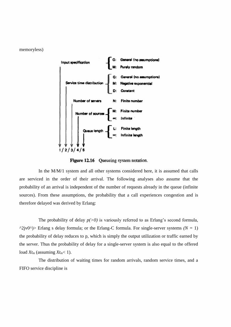
To simplify the characterization of particular systems, queuing theorists have adopted

a concise notation for classifying various types of delay systems. This notation, which was

introduced by D. G. Kendall, uses letter abbreviations to identify alternatives in each of the

categories listed. Although the discussions in this book do not rely on this notation, it is

introduced and used occasionally so the reader can relate the following discussions to classical

queuing theory models. The interpretation of each letter is specified in Figure 12.16.

The specification format presented in Figure 12.16 actually represents an extension of

the format commonly used by most queuing theorists. Thus this format is sometimes

abbreviated by eliminating the last one or two entries. When these entries are eliminated,

infinite case specifications are assumed. For example, a single-server system with random input

and negative exponential service times is usually specified as M/M/l. Both the number of

sources and the permissible queue length are assumed infinite.

Exponential Service Times

The simplest delay system to analyze is a system with random arrivals and negative exponential

service times: M/M/N. Recall that a random arrival distribution is one with negative exponential

interarrival times. Thus in the shorthand notation of queuing theorists, the letter M always refers

to negative exponential distributions (an M is used because a purely random distribution is

memoryless)

In the M/M/1 system and all other systems considered here, it is assumed that calls

are serviced in the order of their arrival. The following analyses also assume that the

probability of an arrival is independent of the number of requests already in the queue (infinite

sources). From these assumptions, the probability that a call experiences congestion and is

therefore delayed was derived by Erlang:

The probability of delay p(>0) is variously referred to as Erlang’s second formula,

^2jv0^)> Erlang s delay formula; or the Erlang-C formula. For single-server systems (N = 1)

the probability of delay reduces to p, which is simply the output utilization or traffic earned by

the server. Thus the probability of delay for a single-server system is also equal to the offered

load Xtm (assuming Xtm< 1).

The distribution of waiting times for random arrivals, random service times, and a

FIFO service discipline is

P(>t) = p(> 0)eHN~A)t/,m (12.25)

where p(>0) = probability of delay given in Equation 12.24

tm = average service time of negative exponential service time distribution

Equation 12.25 defines the probability that a call arriving at a randomly chosen

instant is delayed for more than t/tm service times. Figure 12.17 presents the relationship of

Equation 12.25 by displaying the traffic capacities of various numbers of servers as a function

Constant Service Times

This section considers delay systems with random arrivals, constant service times,

and a single server (M/D/1). Again, FIFO service disciplines and infinite sources are as-sumed.

The case for multiple servers has been solved [3] but is too involved to include here. Graphs of

multiple-server systems with constant service times are available in reference [15].

The average waiting time for a single server with constant service times is deter-

mined as

where p =A is theserver utilization. Notice thatEquation 12.28producesanaverage

waitingtimethatisexactlyone-halfofthatforasingle-server system withexponential

servicetimes.Exponentialservicetimescausegreater averagedelaysbecause there aretworandom

processes involved in creatingthedelay.Inbothtypesof systems,delays occur when a large burst

of arrivals exceeds the capacity of the servers. With exponential service times, however, long

delays also arise because of excessive service times of just a few arrivals. (Recall that this

aspect of conventional message-switching systems is one of the motivations for breaking

messages up into packets in a packet- switching network.)

If the activity profile of a constant service time system (M/D/1) is compared with the

activity profile of an exponential service time system (M/M/1), the M/D/1 system is seen to be

active for shorter and more frequent periods of time. That is, the M/M/1 system has a higher

variance in the duration of its busy periods. The average activity of both systems is, of course,

equal to the server utilization p. Hence the probability of delay for a single-server system with

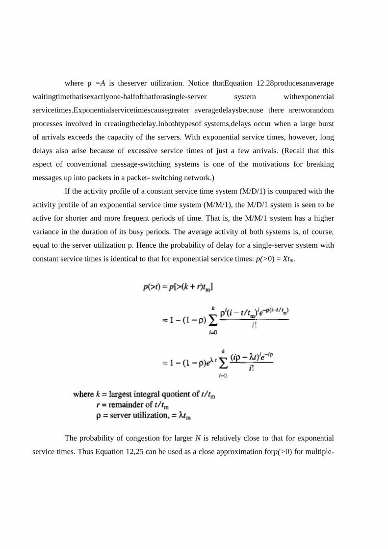
constant service times is identical to that for exponential service times: p(>0) = Xtm.

The probability of congestion for larger N is relatively close to that for exponential

service times. Thus Equation 12,25 can be used as a close approximation forp(>0) for multiple-

server systems with arbitrary service time distributions.

For single-server systems with constant holding times, the probability of delay

greater than an arbitrary value t is

Finite Queues

All of the delay system analyses presented so far have assumed that an arbitrarily

large number of delayed requests could be placed in a queue. In many applications this as-

sumption is invalid. Examples of systems that sometimes have significantly limited queue sizes

are store-and-forward switching nodes (e.g., packet switches and ATM switches), automatic

call distributors, and various types of computer input/output devices. These systems treat

arrivals in three different ways, depending on the number “in the system” at the time of an

arrival:

Immediate service if one or more of N servers are idle

0. Delayed service if all servers are busy and less than L requests are waiting

1. Blocked or no service if the queue of length L is full

In finite-queue systems the arrivals getting blocked are those that would otherwise

experience long delays in a pure delay system. Thus an indication of the blocking probability of

a combined delay and loss system can be determined from the probability that arrivals in pure

delay systems experience delays in excess of some specified value. However, there are two

basic inaccuracies in such an analysis. First, the effect of blocked or lost calls cleared is to

reduce congestion for a period of time and thereby to reduce the delay probabilities for

subsequent arrivals. Second, delay times do not necessarily indicate how many calls are “in the

system.” Normally, queue lengths and blocking probabilities are determined in terms of the

number of waiting requests, not the amount of work or total service time represented by the

requests. With constant service times, there is no ambiguity between the size of a queue and its

implied delay. With exponential service times, however, a given size can represent a wide

range of delay times.

A packet-switching node is an example of a system in which the queue length is most

appropriately determined by implied service time and not by the number of pending requests.

That is, the maximum queue length may be determined by the amount of store-and-forward

memory available for variable-length messages and not by some fixed number of messages.

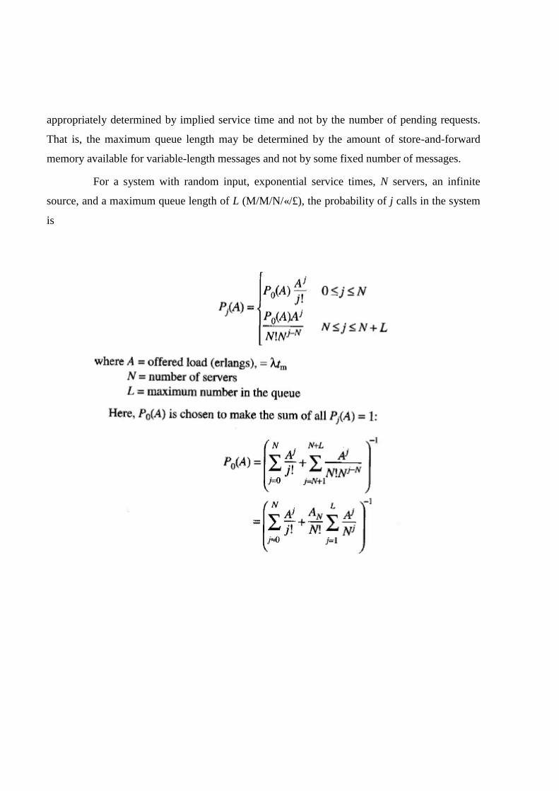
For a system with random input, exponential service times, N servers, an infinite

source, and a maximum queue length of L (M/M/N/«/£), the probability of j calls in the system

is

It is worth noting that if there is no queue (L = 0), these equations reduce to those of the

Erlang loss equation (12.8). If L is infinite, Equation 12.31 reduces to Erlang’s delay

formula, Equation 12.24. Thus these equations represent a general formulation that

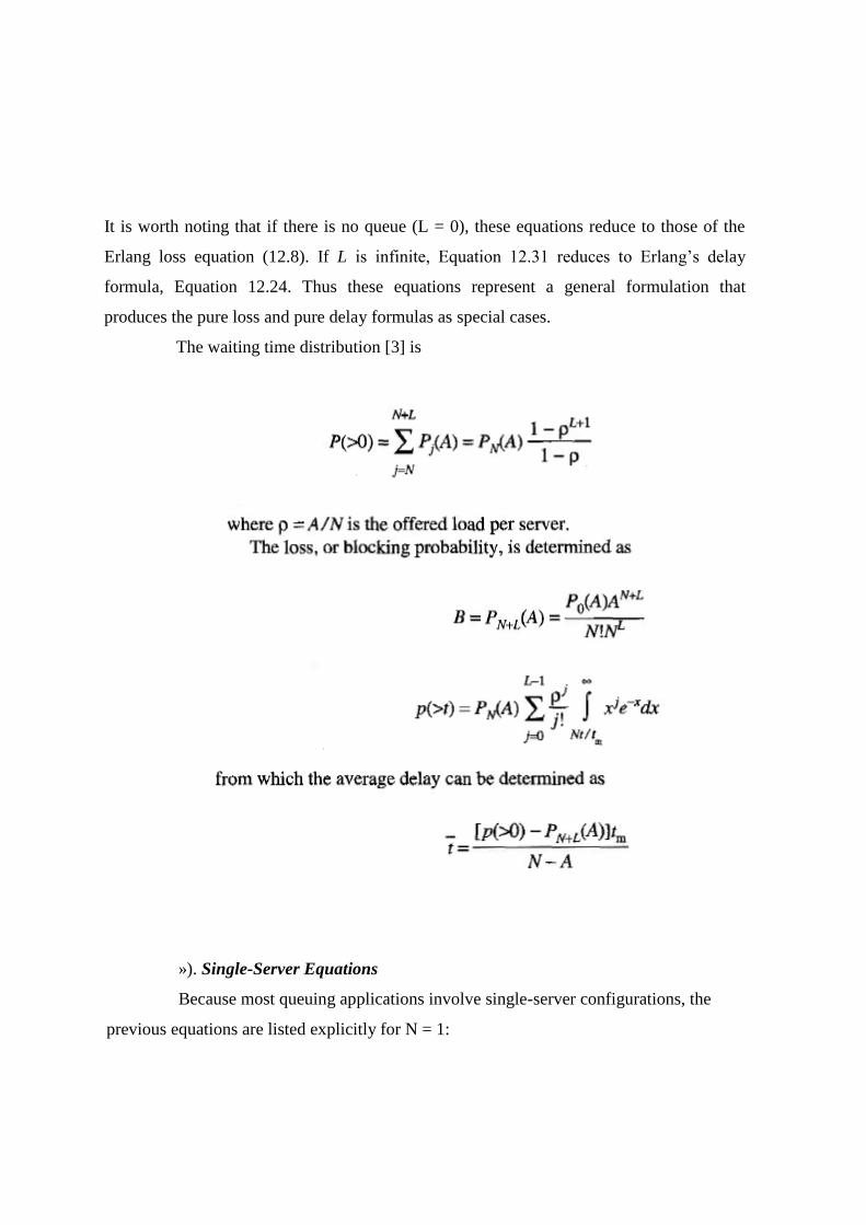
produces the pure loss and pure delay formulas as special cases.

The waiting time distribution [3] is

»). Single-Server Equations

Because most queuing applications involve single-server configurations, the

previous equations are listed explicitly for N = 1:

, Prob(y calls in system) (12.30):

The blocking probability of a single-server system (N = 1) is plotted in Figure

When using Figure 12.19, keep in mind that the blocking probability is determined by

the number of waiting calls and not by the associated service time. Furthermore, since

the curves of Figure 12.19 are based on exponential service times, they overestimate the

blocking probabilities of constant holding time systems (e.g., fixed-length packet

networks). However, if fixed-length packets arise primarily from longer, exponentially

distributed messages, the arrivals are no longer independent, and the use of Figure 12.19

(or Equation 12.38) as a conservative analysis is more appropriate.

ATM Cell Queues

Analysis of queuing delays and cell loss in an ATM switching node is

complicated. The cells have a fixed length of 53 bytes so it would seem that a constant

service time analysis would be appropriate. This assumption is valid for voice traffic

inserted onto wide-bandwidth signals such as 155-Mbps STS-ls. In this case the service

time is much shorter that the duration of a speech burst (e.g., 2.7 (isec versus several tens

of milliseconds). Even though correlated arrivals occur from individual sources, the arrival

times are separated by many thousands of service times so they appear independent.

When ATM voice is carried in CBR trunk groups, a different situation results. In

this case the service times of the voice cells may be only slightly smaller than the interval

between voice cell generation, and the average delay would indicate that two or more cells

from the same source could be present in the queue at one time. Thus, a queuing analysis

that assumes exponentially distributed service times is more appropriate even though the

variable-length talk spurts are broken up into fixed-length cells.

Tandem Queues

All of the equations provided in previous sections for delay system analysis

have dealt with the performance of a single queue. In many applications a service

Tandem queues

request undergoes several stages of processing, each one of which involves queuing. Thus

it is often desirable to analyze the performance of a system with a number of queues in

series. Figure 12.20 depicts a series of queues that receive, as inputs, locally generated

requests and outputs from other queues. Two principal examples of applications with

tandem queues are data processing systems and store-and-forward switching networks.

Researchers in queuing theory have not been generally successful in deriving

formulas for the performance of tandem queues. Often, simulation is used to analyze a

complex arrangement of interdependent queues arising in systems like store-and-for- ward

networks. Simulation has the advantage that special aspects of a network’s operation—like

routing and flow control—can be included in the simulation model. The main

disadvantages of simulation are expense and, often, less visibility into the dependence of

system performance on various design parameters.

One tandem queuing problem that has been solved [19] is for random inputs and

random (negative exponential) holding times for all queues. The solution of this system is

based on the following theorem: In a delay system with purely random arrivals and

negative exponential holding times, the instants at which calls terminate is also a negative

exponential distribution.

The significance of this theorem is that outputs from an M/M/N system have sta-

tistical properties that are identical to its inputs. Thus a queuing process in one stage does

not affect the arrival process in a subsequent stage, and all queues can be analyzed

independently. Specifically, if a delay system with N servers has exponentially distributed.