unit ix - probability distributionsjmpcollege.org/adminpanel/adminupload/studymaterial... · the...
TRANSCRIPT

F.Y.B.COM HANDBOOK OF MATHEMATICAL & STATISTICAL TECHNIQUE
Prepared by Asso.Prof. Dr. Dilip M Patil, J.M.PATEL COLLEGE GOREGAON(W) Page 1
UNIT IX - PROBABILITY DISTRIBUTIONS
BINOMIAL DISTRIBUTION
Bernoulli Trial- A random trial which produces only two possible results termed as
‘Success’ & ‘Failure’ is called as a Bernoulli trial.
Examples of a Bernoulli trial-
When a coin is tossed only 2 possible outcomes Head & Tail
When a cubic die is rolled down there can be only 2 possible outcomes, ‘ A six’ or
‘Not a six’
When a student is examined in the class there can be only 2 possible results ‘Pass’
& ‘Fail’
Students can list out some more situations where results can be divided as ‘Success’
defined and the corresponding ‘Failure’
When n no of such trials are performed independently a variable X defined as the
‘Number of Successes’ is called a Binomial variable.
Hence, a random variable is Binomial when the situation/trial has only two
possibilities like Yes/No Accept/Reject. These trials are called as Bernoulli trials.
Variable X denotes the number of successes in n trials. For example in the experiment
of 10 throws of a cubic die no of times 6 dots appear. It can be 0,1,2,3,4,5,6,7,8,9, or 10.
The probability values of X are calculated by the formula,
P(x) = nCx p
x q
(n-x) where x takes values from 0 to n
p= Probability success defined, q= 1-p for example in the throw of single cubic die,
p= Probability of getting six dots =1/6 & so q= 5/6.
Mean & Variance of binomial distribution are np & npq respectively.
Hence, Mean(X) =nxp & Variance(X)= nxpxq.
Therefore, for the experiment of 10 throws of cubic coin we have n=10 p=1/6 & q=5/6
Hence Mean(X) =10x1/6= 10
6 & Var(X) = 10x
1
6x
5
6=
50
36
F.Y.B.COM HANDBOOK OF MATHEMATICAL & STATISTICAL TECHNIQUE
Prepared by Asso.Prof. Dr. Dilip M Patil, J.M.PATEL COLLEGE GOREGAON(W) Page 2
SOLVED EXAMPLES-
1. A r.v. X follows binomial distribution with n=4 & p= 0.4, calculate
a) P(X=2) b) P(X≤ 1) c) P(X>2)
For the binomial distribution,
p(x) = nCx p
x (q)
(n-x)
a) P(X=2) = 4C2 (0.4)
2 (0.6)
2=
4 3
2 1
x
xx0.4x0.4x0.6x0.6=
b) P(X≤ 1)= P(X=0)+ P(X=1)
= 4C0 (0.4)
2 (0.6)
4+
4C1 (0.4)
1 (0.6)
3
=1x1x0.6 4times + 4x0.4x0.6 3times=
c) P(X>2)= P(X=3)+ P(X=4)
= 4C3 (0.4)
3 (0.6)
1+
4C4 (0.4)
4 (0.6)
0
=4x0.4 3timesx0.6 + 1x0.4 4 timesx1=0.1792
2. It is known that p=40% of the members of the club are ladies. What is the probability of
getting 3 or 4 ladies in the group of randomly selected 6 members of the club?
Solution: Here we can note that, a member selected can be either a Male or a Female hence it
is a Bernoulli trial & variable X: No of lady members is a binomial variable with n=6, p=0.4
& q=0.6
Now, probability of X is calculated by the formula
p(x) = 6Cx 0.4
x (0.6)
(6-x) where x takes values from 0,1,2,3,4,5 & 6.
Therefore,
Prob(3 or 4 ladies members) = P(X=3) + P(X=4)
= 6C3 0.4
3 (0.6)
(6-3)+
6C40.4
4 (0.6)
(6-2)
= 20x0.064x0.216 + 15x0.0256x0.36
= 0.4147= 41.47% chanceof 3 or 4 lady members.
3. When every 3rd
students in the class has studied in English medium. Find the
probability of having exactly 4 students from English in randomly selected group of 5
students in the class.
Solution: A student selected is either English medium or not from English medium hence,
it is a Bernoulli trial & variable X is binomial with N= 5, p= 1
3 (every 3
rd) & q=
2
3.

F.Y.B.COM HANDBOOK OF MATHEMATICAL & STATISTICAL TECHNIQUE
Prepared by Asso.Prof. Dr. Dilip M Patil, J.M.PATEL COLLEGE GOREGAON(W) Page 3
Probability formula, P(x) = 5Cx (1/3)
x (2/3)
(5-x) where x takes values from 0,1,2,3,4 & 5.
Therefore,
Prob (4 students from English medium)= P(X=4)
=5C4 (1/3)
4 (2/3)
1
= 5x 1
3x
1
3x
1
3x
1
3x
2
3=
10
243 = 0.0411= 4.11% chance
4. In the class of 50 students p=40% are good at singing. What is the probability that out
of randomly selected n=5 students only x=2 are good in singing?
Solution: Here we can note that, a student selected can be either a singer or not a singer.
Hence, it is a Bernoulli trial & variable X: No of Singer follows a binomial distribution with
n=5, p=P(Singer)= 40%= 0.4 & so q=0.6
Now, probability of X is calculated by the formula
p(x) = p(x) = nCx (p)
x (q)
(n-x) where x takes values from 0,1,2,3,4,5 & 6.
Therefore,
P(only 2 singer) = p(x)= 5C2 (0.4)
2 (0.6)
3
= 5 4 3
3 2 1
x x
x xx0.4x0.4x0.6x0.6x0.6=
5. The mean & variance of a binomial distribution are np=4 &npq=4/3 respectively,
calculate P(X=3). Find n & p, hence calculate P(X=3)
Solution: Given variable X is binomial. Hence Mean(X)=nxp =4 & Var(X) = nxpxq= 4/3
Consider, nxpxq
nxp= q=
4 / 3
4=
1
3. It gives q=
1
3 & so p= 1-
1
3=
2
3.
Also since nxp = 4/3 & p = 2
3we get, n=
4
3 x
3
2= 8
Now, P)X=3) = 8C3 (2/3)
3 (1/3)
5
=8 7 6
3 2 1
x x
x xx
2
3x
2
3x
2
3x
1
3x
1
3x
1
3x
1
3x
1
3= 0.0682= 6.82% chance

F.Y.B.COM HANDBOOK OF MATHEMATICAL & STATISTICAL TECHNIQUE
Prepared by Asso.Prof. Dr. Dilip M Patil, J.M.PATEL COLLEGE GOREGAON(W) Page 4
POISSON DISTRIBUTION
Similar to ‘Binomial’ distribution, ‘Poisson’ distribution is also the case of Bernoulli
trial, but the difference is that, here n: No of trials is sufficiently large (more than 30) and p:
probability of success is very small. In other words Poisson distribution is applicable when the
chance of success is very rare like proportion of defective item in a good quality system.
Therefore, a random variable X is Poisson distribution with parameter ‘m’ if it’s
probability formula is written as,
p(x)= !
m xe m
x
where, m=np & x= 0,1,2,3,-----
p= Probability of ‘Success defined’ & n: No of trials
For the Poisson distribution: Mean = Variance = m parameter
SOLVED EXAMPLES-
1. A r.v. X follows Poisson distribution with Mean m =1.5. Calculate
a) P(X=2) b) P(X≤ 1) c) P(X>1)
For the binomial distribution,
p(x) = !
m xe m
x
where m=1.5
Now, P(X=2) = 1.5 21.5
2!
e= 0.2510
b) P(X≤ 1)= P(X=0)+ P(X=1)
= 1.5 01.5
0!
e+
1.5 11.5
1!
e=0.2231+ 0.3346= 0.5577
c) P(X>1)= 1- P(X≤ 1) = 1-0.5577 = 0.4423
2. It is known that maximum 0.1% of the items produced in the workshop are defectivies.
Find the probability of getting at most 2 defectives in the lot of 250 items inspected
randomly.( Given 0.5e = 0.6065
Solution: Here, we can note that, proportion of defective items is very small p= 0.1% and the
no of trials n=500 is sufficiently large. Hence the variable
X- No of defectives follows a Poisson distribution with Mean m= np = 500x0.1%=0.5
And the probability function as,
p(x) = !
m xe m
x
where m=0.5

F.Y.B.COM HANDBOOK OF MATHEMATICAL & STATISTICAL TECHNIQUE
Prepared by Asso.Prof. Dr. Dilip M Patil, J.M.PATEL COLLEGE GOREGAON(W) Page 5
Now probability of getting at most 2 defectives means P(X≤ 2)
P(X≤ 2) = P(X=0)+ P(X=1)+ P(X=2)
= 0.5 00.5
0!
e+
0.5 10.5
1!
e+
0.5 20.5
2!
e
=0.6065+ 0.3032+ 0.0758 = 0.9855
3. For a r.v X with Poisson distribution 4P(X=0) = P(X=1). Calculate P(X≥2).
Solution: Given r.v. X follows Poisson distribution hence, it’s probability function is
p(x) = !
m xe m
x
where m= is the parameter
According to information, 4P(X=0) = P(X=1). It means,
4x0
0!
me m
=1
1!
me m
i.e. 4 me = me m gives m=4
Therefore, with m=4 the probability function becomes,
p(x) =4 4
!
xe
x
Now,
P(X≥2) = 1- P(X≤ 1)
= 1- {P(X=0)+ P(X=1)}
= 1-{ 4 04
0!
e+
4 14
1!
e}
= 1-{ 4e + 4x 4e }
= 1- {0.0183+4x0.183}= 1- 0.0915 = 0.9085.

F.Y.B.COM HANDBOOK OF MATHEMATICAL & STATISTICAL TECHNIQUE
Prepared by Asso.Prof. Dr. Dilip M Patil, J.M.PATEL COLLEGE GOREGAON(W) Page 6
NORMAL DISTRIBUTION
Normal distribution deals with the calculation of probabilities for a continuous random
variable like Height of players, Marks of students, or Wages of workers. We define the normal
distribution as follows.
A continuous random variable X is said follow a normal distribution with parameters and 6,
written as X N( , 62) if it’s probability function is given by
p(x)=1
6 2e
xp
1 x( )
2
2
x, R, 6>0
= 0 otherwise.
Where the constants are
= Mean(X); = S.D.(X)
= 3.142 and e= 2.718 (appro).
Before we learn to calculate the probabilities on normal distribution, we state the
characteristics of the normal distribution stated below.
Characteristics of the normal distribution
The graph of normal distribution is a bell shaped curve.
The area under the curve reads the probabilities of normal distribution hence total area
is 1 (one).
The curve is symmetric about it’s mean . Hence,
Area on l.h.s. of = Area on r.h.s. of = 0.5. Since area reads probability,
P(X< ) = P(X> ) = 0.5= 50%.
Hence mean divides the curve into two equal parts so it is also the median.
The curve has it’s maximum height at x = , therefore it the mode of the distribution.
Hence for normal distribution Mean = Median = Mode =
For the probability calculations, we define the variable Z = x
. .
Mean
S D
=
x
Mean (Z) = 0 and S.D.(Z)= 1. Z is called a standard normal variable (s.n.v.)
Also P (X) = P (Z) = Area (Z). The area (probability) values of z are tabulated.
The lower (Q1) and upper quartiles (Q3) are equidistant from the mean .
i.e. -Q1 = Q3- = 1 3
2
Q Q

F.Y.B.COM HANDBOOK OF MATHEMATICAL & STATISTICAL TECHNIQUE
Prepared by Asso.Prof. Dr. Dilip M Patil, J.M.PATEL COLLEGE GOREGAON(W) Page 7
The mean deviation (M.D.) of normal distribution is4
5 =80%(SD)
The quartile deviation (Q.D.) of normal distribution is 0.67 .
Area under the normal curve between
(i) + is 68.27% (ii) + 2 is 95.45% (iii) + 3 is 99.73%.
1. A continuous random variable X follows a normal distribution with mean 50 and S.D.
of 10. Find the following probabilities for X,
a) P (X55) b) P(45X60) c) P(X45).
Solution: For the normal variable X , we have
Mean (X)= = 50 and standard deviation = 6= 5.
... X (N (, 6
2) = N (50, 10
2).
We define the variable Z =x
=
x 50
5
Mean (Z) = 0 and S.D.(Z)= 1. Z is called a standard normal variable (s.n.v.)
Also P (X) = P (Z) = Area (Z).
a) P (X55)= P(x 50
5
55 50
5
)
= P(Z1)
= Area r.h.s. of +1
= 0.5- Area from 0 to 1
= 0.5-0.3413 = 0.1587.
Graph of Z
F.Y.B.COM HANDBOOK OF MATHEMATICAL & STATISTICAL TECHNIQUE
Prepared by Asso.Prof. Dr. Dilip M Patil, J.M.PATEL COLLEGE GOREGAON(W) Page 8
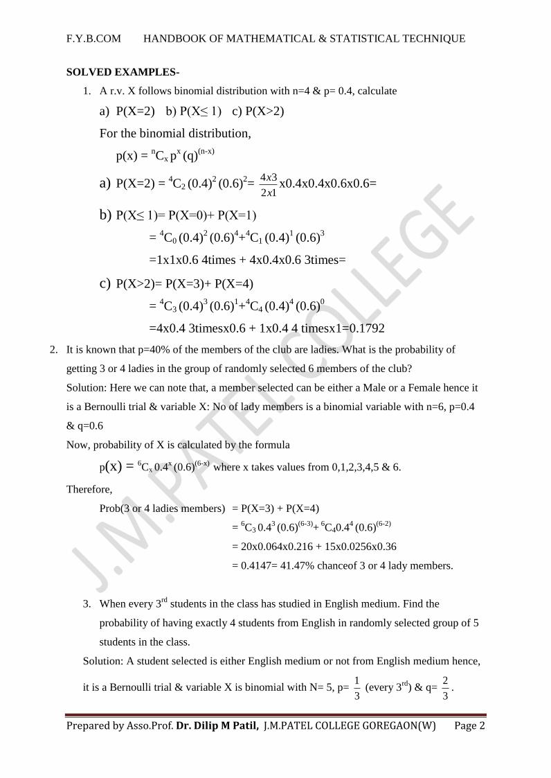
b) P(45X60)
= P(45 50
5
x 50
5
60 50
5
)
= P(-1 Z 2)
= Area between -1 & +2
= Area from -1 to 0+ Area from 0 to 2.
= 0.3413 + 0.4772 = 0.8185.
c) P(X45)=P(x 50
5
45 50
5
)
= P(Z-1)= Area on l.h.s. of -1.
= 0.5 - Area from -1 to 0
= 0.5 - 0.3413 = 0.1587.
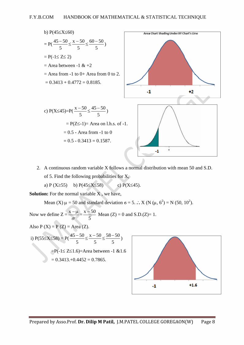
2. A continuous random variable X follows a normal distribution with mean 50 and S.D.
of 5. Find the following probabilities for X,
a) P (X55) b) P(45X58) c) P(X45).
Solution: For the normal variable X , we have,
Mean (X) = 50 and standard deviation ϭ = 5. ... X (N (, 6
2) = N (50, 10
2).
Now we define Z =x
=
x 50
5
Mean (Z) = 0 and S.D.(Z)= 1.
Also P (X) = P (Z) = Area (Z).
i) P(55X58) = P(45 50
5
x 50
5
58 50
5
)
=P(-1 Z1.6)=Area between -1 &1.6
= 0.3413.+0.4452 = 0.7865.

F.Y.B.COM HANDBOOK OF MATHEMATICAL & STATISTICAL TECHNIQUE
Prepared by Asso.Prof. Dr. Dilip M Patil, J.M.PATEL COLLEGE GOREGAON(W) Page 9
ii) P (X≤40)= P(x 50
5
≤
40 50
5
)
= P(Z≤ -2) = Area l.h.s. of -2
= 0.5- Area from 0 to -2
= 0.5-0.4773 = 0.0227.
3. The marks of 150 students in the class is said to follow a normal with mean 60 and
S.D. of 10. Find, the expected no of students scoring marks below 45.Percentage of
students scoring marks between 55 and 70.
Solution: Let X: Marks of students;
Mean(X) = 60 and S.D.(X) = 6 = 10.
X has normal distribution with =60 and 6 = 10.
i.e. X( N ( , 62) = N (60, 10
2). We define Z=
x
=
x 60
10
.
... Mean (Z) = 0 and S.D.(Z)= 1. Z is called a standard normal variable (s.n.v.)
Also P (X) = P (Z) = Area (Z).
Now, to find the expected no of students scoring marks below 45, we find
P(marks less than 45) = P(X 45)
=.P(x 60
10
45 60
10
)
= P(Z -1.5)
= Area on l.h.s. of -1.5.
= 0.5 - Area from -1.5 to 0
= 0.5 - 0.4332
= 0.0668 = 6.68%.
Expected no of students = 6.68% (150) =10
Similarly, to find percentage of students scoring marks between 55 and 70.
Consider, P(marks between 55 and 70)

F.Y.B.COM HANDBOOK OF MATHEMATICAL & STATISTICAL TECHNIQUE
Prepared by Asso.Prof. Dr. Dilip M Patil, J.M.PATEL COLLEGE GOREGAON(W) Page 10
P(55X70) =P(55 60
10
x 60
10
70 60
10
)
= P(-0.5 Z 1)
= Area between -0.5 & +1
= Area from -0.5 to 0+Area from 0 to 1.
= 0.1915 + 0.3413= 0.5328 = 53.28%.
... 53.28% students have scored marks between 55
and 70.
4. The daily wages of 300 workers in a factory are normally distributed with the average
wages of Rs.2500 and S.D. of wages equals to Rs.500. Find the percentage of workers
earning wages between Rs.3000 and Rs.4000. Also find the wages of the lowest paid
worker in the group of highest paid 30% workers.
Solution: Let r.v. X denotes the wages of a worker.
Mean(X) = 2500 and S.D.(X) = = 500.
... X has normal distribution with =2500 and = 500.
i.e. X( N ( , 2) = N (2500, 500
2)
We define Z=x
=
x 2500
500
... Mean (Z) = 0 and S.D.(Z)= 1. Z is called a standard normal variable (s.n.v.)
Also P (X) = P (Z) = Area (Z).
Now, to find the percentage of workers earning wages between Rs 3000 and Rs 4000.
Consider, P(wages between Rs.3000 and Rs 4000)
= P(3000X4000)
=P(3000 2500
500
x 2500
500
4000 2500
500
)
= P (1 Z 1.5)
= Area between +1 & +1.5
= Area from 0 to 1.5 - Area from 0 to 1.
= 0.4332 - 0.3413= 0.0919 = 9.19%.
... 9.91% workers are earning wages between Rs3000 and Rs4000.
Now, let the wages of the lowest paid worker in the group of highest paid 30% workers be h.
P(wages greater than h) =30%=0.3 i.e. P(X h) = 0.3.

F.Y.B.COM HANDBOOK OF MATHEMATICAL & STATISTICAL TECHNIQUE
Prepared by Asso.Prof. Dr. Dilip M Patil, J.M.PATEL COLLEGE GOREGAON(W) Page 11
Consider,
P(X h) = P (x 2500
500
h 2500
500
= t say)
i.e. P(Z t) = 0.3.
... Area on r.h.s. of t =0.3 (it is greater than 0
i.e. positive.( since area on r.h.s.< 0.5) area
from 0 to t = 0.2.
Now from the normal area table, area from 0
to 0.52 is 0.2.
Hence, t = 0.52 (t=h 2500
500
= 0.52) i.e. h = 2500 + 500(0.52) =2500+260 = 2760.
Therefore, the wages of the lowest paid worker in the group of highest paid 30% workers are
Rs. 2760.
EXERCISE
1. For a binomial variable X with n=5 & p= 0.6, calculate
a) P(X=2) b) P(X≤ 1) c) P(X>3)
2. It is known that p=40% of the students in the class are girls. What is the probability
that randomly selected 6 students includes at least 4 girls?
3. The mean & variance of a binomial distribution are 9/2 & 9/8 respectively,
Calculate P(X=3).
4. A continuous random variable X follows a normal distribution with mean 50 and S.D.
of 10. Find the following probabilities for X,
a) P (X55) b) P (45X 60) c) P(X 45)
5. The marks of 150 students in the class is said to follow a normal with mean 60 and
S.D. of 10. Find, the expected no of students scoring marks below 45.Percentage of
students scoring marks between 55 and 70.
6. The height of 250 soldiers in a military camp confirms a normal distribution with
mean height of 155cms.and S.D. of 20cms. Find the proportion of soldiers with height
above 170 cms. Also find the height of the shortest soldier in the group of tallest 20%
soldiers.
7. The daily wages of 300 workers in a factory are normally distributed with the average
wages of Rs.2500 and S.D. of wages equals to Rs.500. Find the percentage of workers
earning wages between Rs.3000 and Rs.4000. Also find the wages of the highest paid
worker in the group of lowest paid 30% workers.

F.Y.B.COM HANDBOOK OF MATHEMATICAL & STATISTICAL TECHNIQUE
Prepared by Asso.Prof. Dr. Dilip M Patil, J.M.PATEL COLLEGE GOREGAON(W) Page 12
8. A normal distribution has mean = 15 and 6= 5. Find the following probabilities.
P(X20) P(10X 17.5) P(X 12).
9. A continuous random variable X follows a normal distribution with mean 50 and S.D.
of 10. Find the following probabilities for X,
a) P (X 55) b) P(45X 60) c) P(X 45).
10. The height of 250 soldiers in a military camp confirms a normal distribution with
mean height of 155cms.and S.D. of 20cms. Find the proportion of soldiers with height
above 170 cms. Also find the height of the shortest soldier in the group of tallest 20%
soldiers.
11. The daily wages of 300 workers in a factory are normally distributed with the average
wages of Rs.2500 and S.D. of wages equals to Rs.500.
* Find the percentage of workers earning wages between Rs.3000 and Rs.3750.
* Find the approximate no of workers earning wages below Rs3250/-
* Also find the wages of the lowest paid worker in the group of highest paid
30% workers.