UNIT III: COMPETITIVE STRATEGY

• Monopoly• Oligopoly• Strategic Behavior

7/19

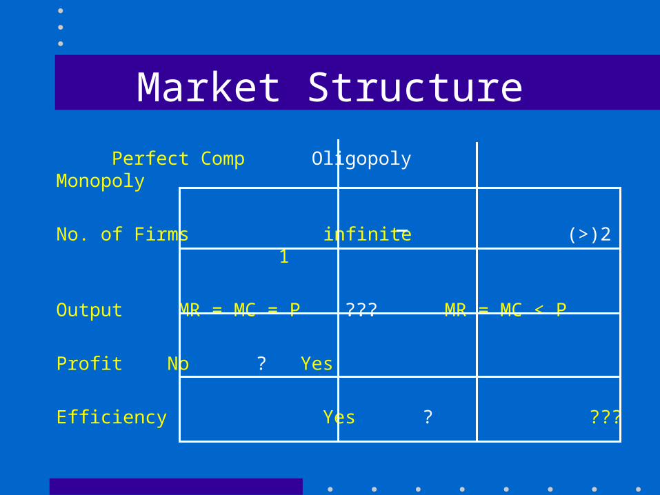
Market Structure

Perfect Comp Oligopoly Monopoly

No. of Firms infinite (>)2 1

Output MR = MC = P ??? MR = MC < P

Profit No ? Yes

Efficiency Yes ? ???

Oligopoly

We have no general theory of oligopoly. Rather, there are a variety of models, differing in assumptions about strategic behavior and information conditions.

All the models feature a tension between:

– Collusion: maximize joint profits– Competition: capture a larger share of the pie

Duopoly Models

• Cournot Duopoly

• Nash Equilibrium

• Leader/Follower Model

• Price Competition

Duopoly Models

• Cournot Duopoly

• Nash Equilibrium

• Stackelberg Duopoly

• Bertrand Duopoly

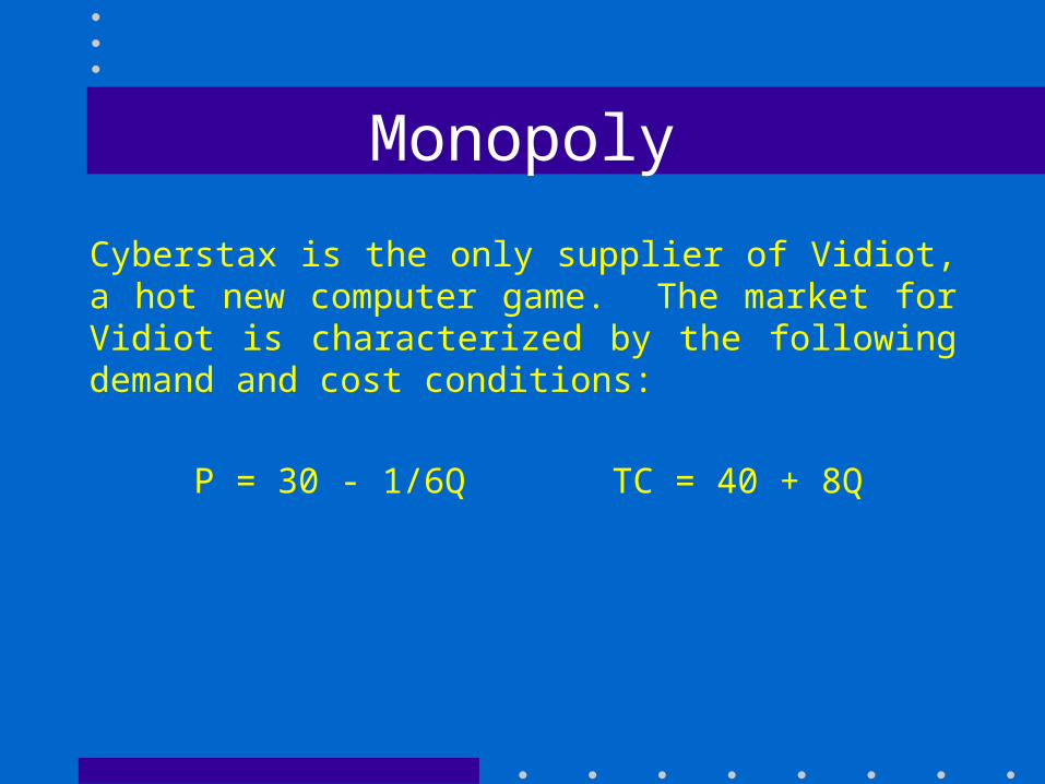
Monopoly

Cyberstax is the only supplier of Vidiot, a hot new computer game. The market for Vidiot is characterized by the following demand and cost conditions:

 

P = 30 - 1/6Q TC = 40 + 8Q

 

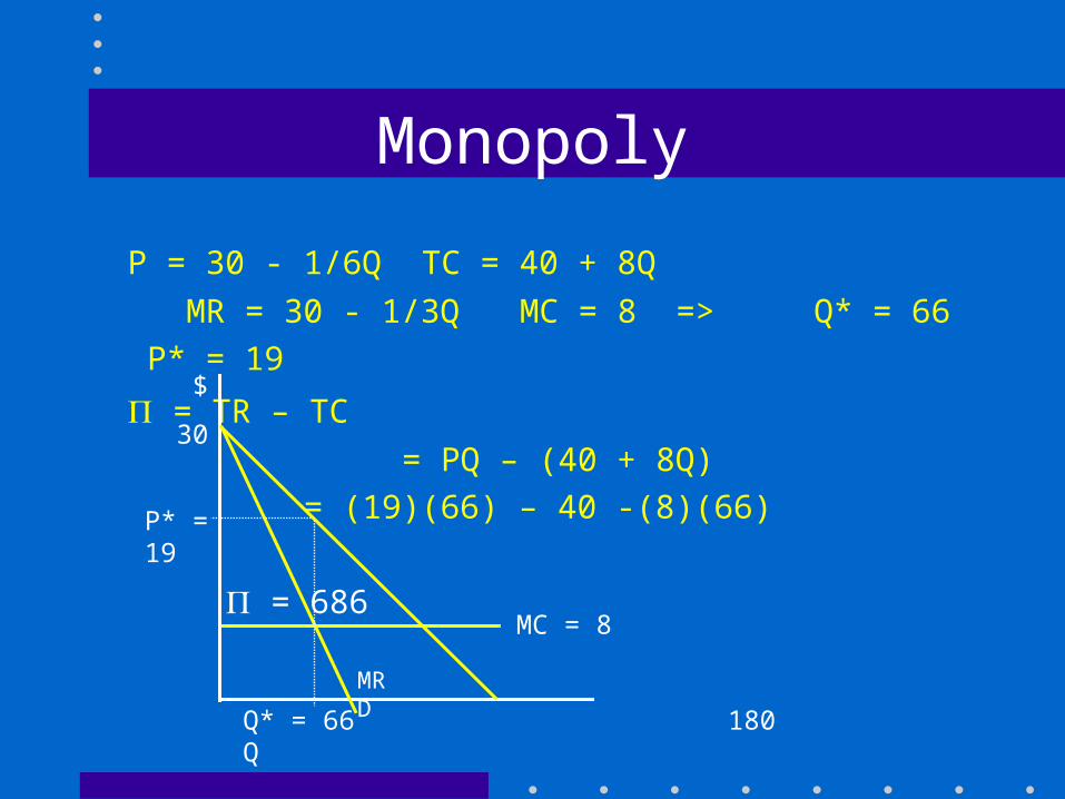
Monopoly

P = 30 - 1/6Q TC = 40 + 8Q

MR = 30 - 1/3Q MC = 8 => Q* = 66

P* = 19

= TR – TC

= PQ – (40 + 8Q)

= (19)(66) – 40 -(8)(66)

= 686

$

30

P* = 19

Q* = 66 180 Q

MC = 8

MR D

Duopoly

Megacorp is thinking of moving into the Vidiot business with a clone which is indistinguishable from the original. It has access to the same production technology, reflected in the following total cost function:

 TC2 = 40 + 8q2

 Will Megacorp enter the market?

What is its profit maximizing level of output?

Duopoly

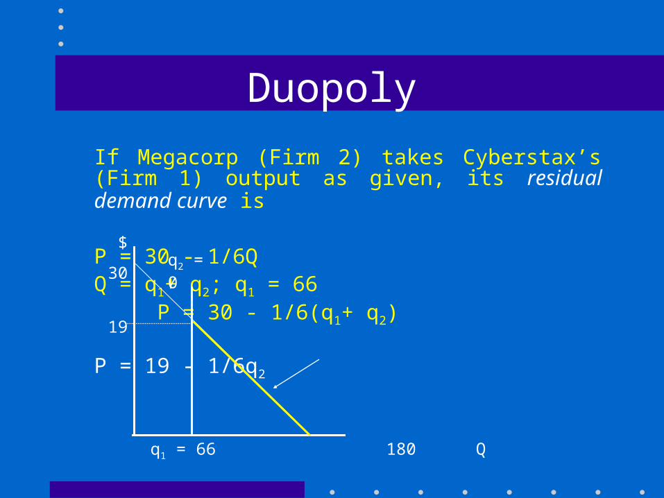
If Megacorp (Firm 2) takes Cyberstax’s (Firm 1) output as given, its residual demand curve is

P = 30 - 1/6QQ = q1+ q2; q1 = 66

P = 30 - 1/6(q1+ q2)

P = 19 - 1/6q2

$

30

19

q2 = 0

q1 = 66 180 Q

Duopoly

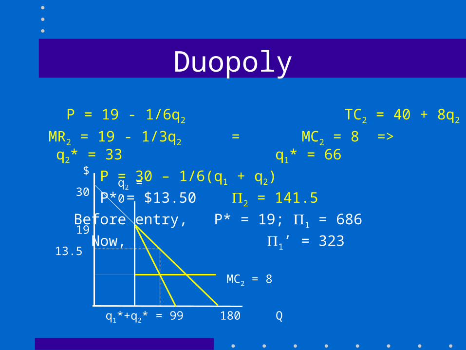
P = 19 - 1/6q2 TC2 = 40 + 8q2

MR2 = 19 - 1/3q2 = MC2 = 8 => q2* = 33 q1* = 66

P = 30 – 1/6(q1 + q2)

P* = $13.50 2 = 141.5

Before entry, P* = 19; 1 = 686

Now, 1’ = 323 ow, C‘ = 297

q1*+q2* = 99 180 Q

$

30

19

13.5

q2 = 0

MC2 = 8

Duopoly

What will happen now that Cyberstax knows there is a competitor? Will it change its level of output?

How will Megacorp respond? Where will this process end?

Cournot Duopoly

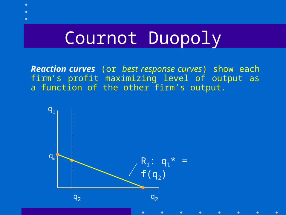
Reaction curves (or best response curves) show each firm’s profit maximizing level of output as a function of the other firm’s output.

q1

qm

q2 q2

R1: q1* = f(q2)

Cournot Duopoly

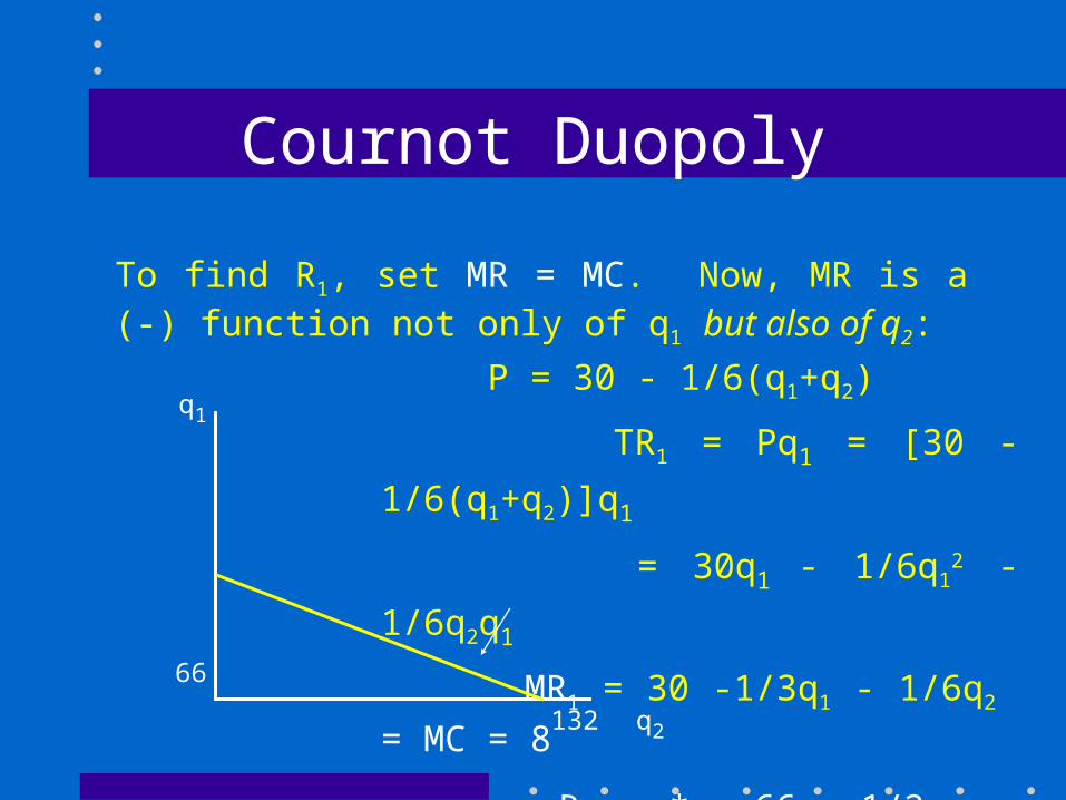
To find R1, set MR = MC. Now, MR is a (-) function not only of q1 but also of q2:

q1

66

132 q2

P = 30 - 1/6(q1+q2)

TR1 = Pq1 = [30 - 1/6(q1+q2)]q1

= 30q1 - 1/6q12 - 1/6q2q1

MR1 = 30 -1/3q1 - 1/6q2 = MC = 8

R1: q1* = 66 – 1/2q2

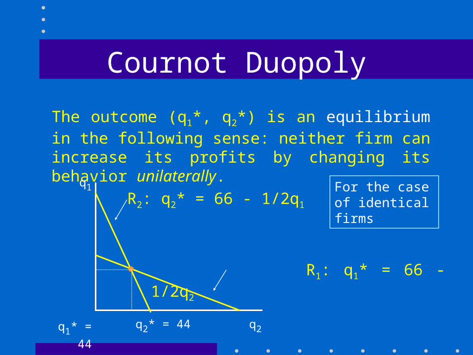
Cournot Duopoly

The outcome (q1*, q2*) is an equilibrium in the following sense: neither firm can increase its profits by changing its behavior unilaterally.

q1

q1* = 44

q2* = 44 q2

R2: q2* = 66 - 1/2q1

R1: q1* = 66 - 1/2q2

For the case of identical firms

Nash Equilibrium

q1

q1* = 44

q2* = 44 q2

R2: q2* = 66 - 1/2q1

R1: q1* = 66 - 1/2q2

For the case of identical firms

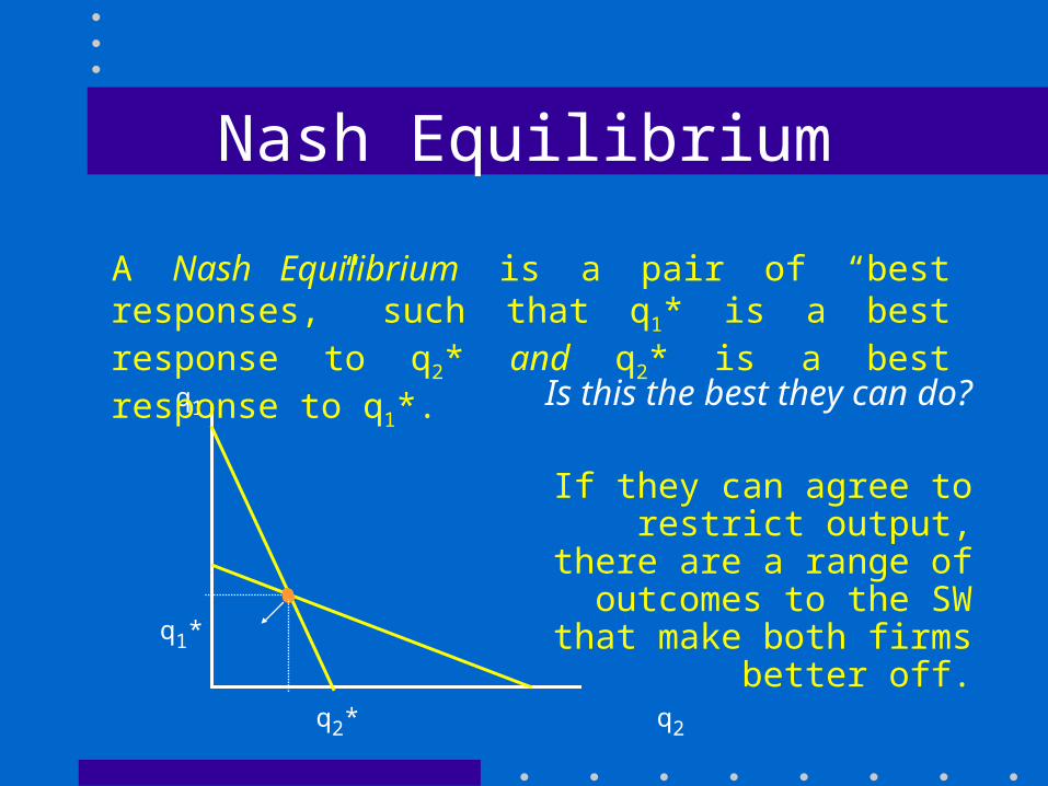
A Nash Equilibrium is a pair of “best responses,” such that q1* is a best response to q2* and q2* is a best response to q1*.

Nash Equilibrium

q1

q1*

q2* q2

Is this the best they can do?

If Firm 1 reduces its output while Firm 2 continues to

produce q2*, the price rises and Firm 2’s profits

increase.

A Nash Equilibrium is a pair of “best responses,” such that q1* is a best response to q2* and q2* is a best response to q1*.

Nash Equilibrium

q1

q1*

q2* q2

Is this the best they can do?

If Firm 2 reduces its output while Firm 1 continues to

produce q1*, the price rises and Firm 1’s profits

increase.

A Nash Equilibrium is a pair of “best responses,” such that q1* is a best response to q2* and q2* is a best response to q1*.

Nash Equilibrium

q1

q1*

q2* q2

Is this the best they can do?

If they can agree to restrict output, there are a range of

outcomes to the SW that make both firms better off.

A Nash Equilibrium is a pair of “best responses,” such that q1* is a best response to q2* and q2* is a best response to q1*.

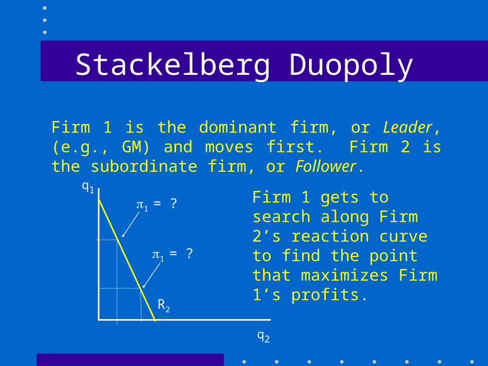
Stackelberg Duopoly

Firm 1 is the dominant firm, or Leader, (e.g., GM) and moves first. Firm 2 is the subordinate firm, or Follower.

q1

q2

R2

Firm 1 gets to search along Firm 2’s reaction curve to find the point that maximizes Firm 1’s profits.1 = ?

1 = ?

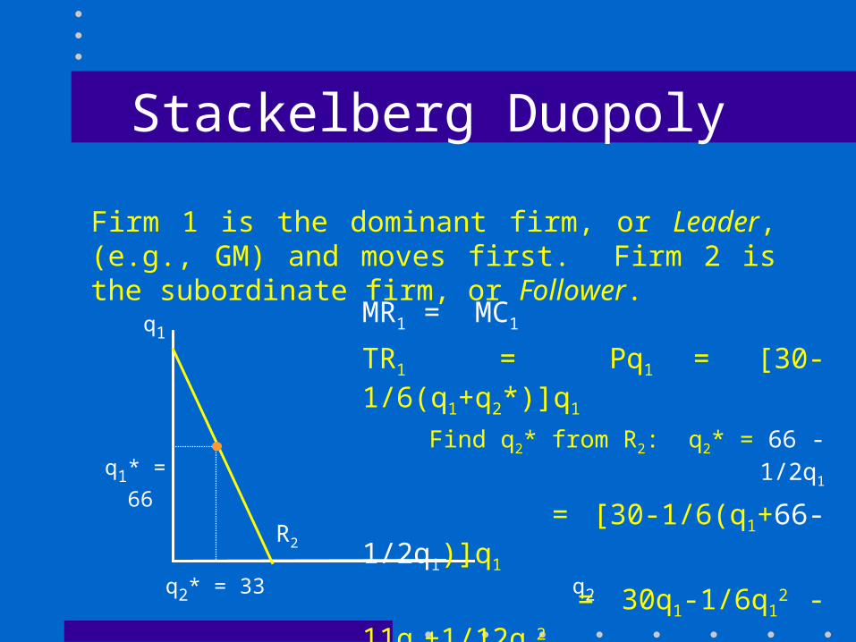
Stackelberg Duopoly

Firm 1 is the dominant firm, or Leader, (e.g., GM) and moves first. Firm 2 is the subordinate firm, or Follower.

q2* = 33 q2

R2

q1

q1* = 66

MR1 = MC1

TR1 = Pq1 = [30-1/6(q1+q2*)]q1

Find q2* from R2: q2* = 66 - 1/2q1

= [30-1/6(q1+66-1/2q1)]q1

= 30q1-1/6q12 -11q1+1/12q1

2

MR1 = 19 -1/6q1 = MC1 = 8

q1* = 66; q2* = 33

Stackelberg Duopoly

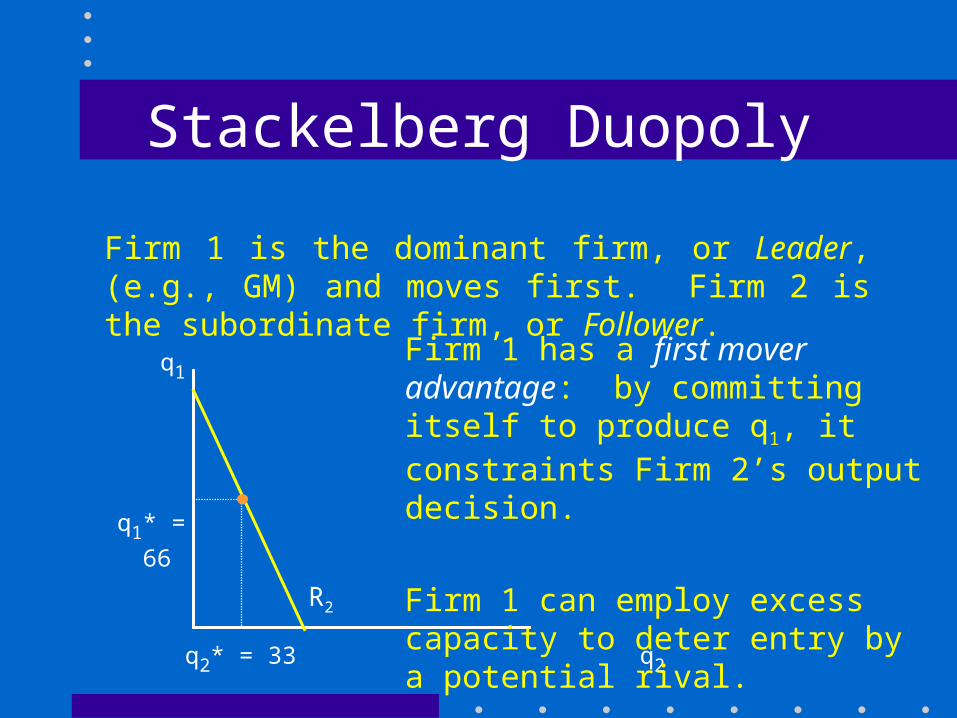
Firm 1 is the dominant firm, or Leader, (e.g., GM) and moves first. Firm 2 is the subordinate firm, or Follower.

q2* = 33 q2

Firm 1 has a first mover advantage: by committing itself to produce q1, it constraints Firm 2’s output decision.

Firm 1 can employ excess capacity to deter entry by a potential rival.

R2

q1

q1* = 66

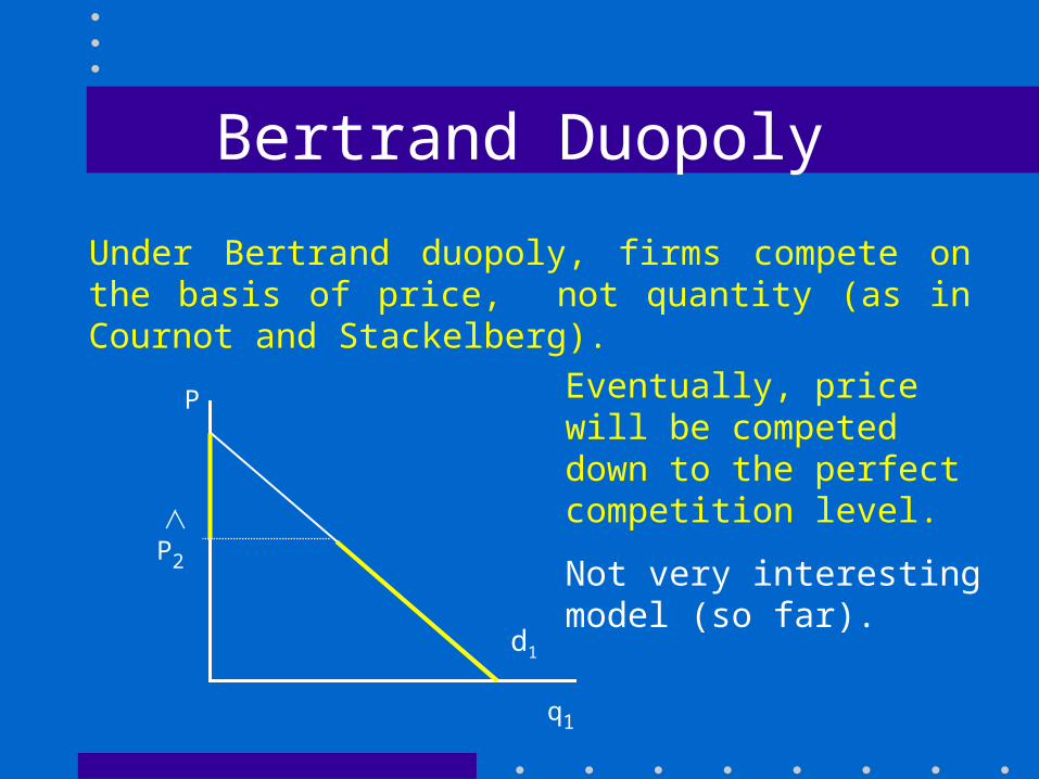
Bertrand Duopoly

Under Bertrand duopoly, firms compete on the basis of price, not quantity (as in Cournot and Stackelberg).

P

P2

q1

If P1 > P2 => q1 = 0

If P1 = P2 => q1 = q2 = ½ Q

If P1 < P2 => q2 = 0

d1

Bertrand Duopoly

Under Bertrand duopoly, firms compete on the basis of price, not quantity (as in Cournot and Stackelberg).

P

P2

q1

Eventually, price will be competed down to the perfect competition level.

Not very interesting model (so far).

d1

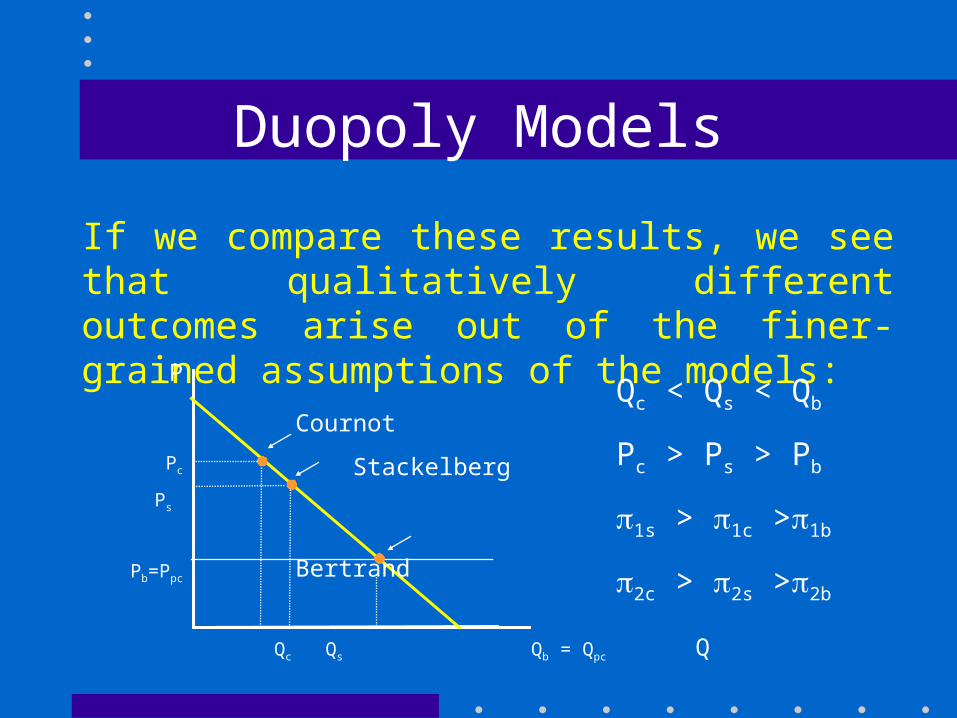
Duopoly Models

If we compare these results, we see that qualitatively different outcomes arise out of the finer-grained assumptions of the models:

P

15.3

13.5

8

c

88 99 132 Q

Cournot

Stackelberg

Bertrand

P = 30 - 1/6Q

TC = 40 + 8q

Duopoly Models

If we compare these results, we see that qualitatively different outcomes arise out of the finer-grained assumptions of the models:

Cournot

Stackelberg

Bertrand

Qc < Qs < Qb

Pc > Ps > Pb

1s > 1c >1b

2c > 2s >2b

P

Pc

Ps

Pb=Ppc

c

Qc Qs Qb = Qpc Q

Duopoly ModelsSummary

Oligopolistic markets are underdetermined by theory. Outcomes depend upon specific assumptions about strategic behavior.

Nash Equilibrium is strategically stable or self-enforcing, b/c no single firm can increase its profits by deviating.

In general, we observe a tension between– Collusion: maximize joint profits– Competition: capture a larger share of the pie

Game Theory

• Game Trees and Matrices

• Games of Chance v. Strategy• The Prisoner’s Dilemma• Dominance Reasoning• Best Response and Nash

Equilibrium• Mixed Strategies

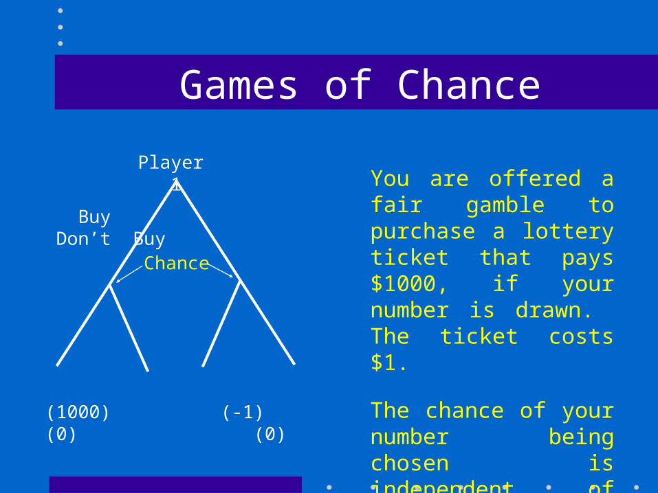
Games of Chance

Buy Don’t Buy

(1000) (-1) (0) (0)

Player 1

Chance

You are offered a fair gamble to purchase a lottery ticket that pays $1000, if your number is drawn. The ticket costs $1.

What would you do?

Games of Chance

Buy Don’t Buy

(1000) (-1) (0) (0)

Player 1

Chance

You are offered a fair gamble to purchase a lottery ticket that pays $1000, if your number is drawn. The ticket costs $1.

The chance of your number being chosen is independent of your decision to buy the ticket.

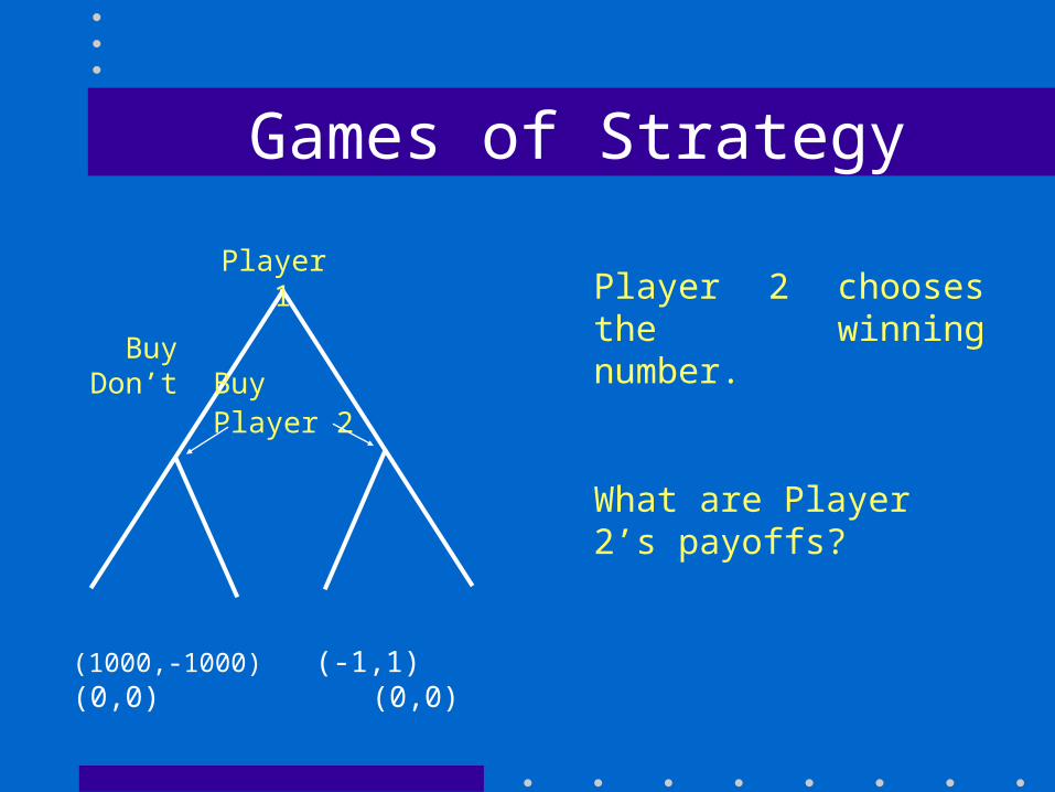
Games of Strategy

Buy Don’t Buy

(1000,-1000) (-1,1) (0,0) (0,0)

Player 1

Player 2

Player 2 chooses the winning number.

What are Player 2’s payoffs?

Games of Strategy

Advertise Don’t

Advertise

A D A D

(10,5) (15,0) (6,8) (20,2)

Firm 1

Firm 2

Duopolists deciding to advertise. Firm 1 moves first. Firm 2 observes Firm 1’s choice and then makes its own choice.

How should the game be played?

Backwards-induction

Games of Strategy

Advertise Don’t

Advertise

A D A D

(10,5) (15,0) (6,8) (20,2)

Firm 1

Firm 2

Duopolists deciding to advertise. The 2 firms move simultaneously. (Firm 2 does not see Firm 1’s choice.)

Imperfect Information.

Information set

Matrix Games

Advertise Don’t

Advertise

A D A D

(10,5) (15,0) (6,8) (20,2)

Firm 1

Firm 2

10, 5 15, 0

6, 8 20, 2

A D

A

D

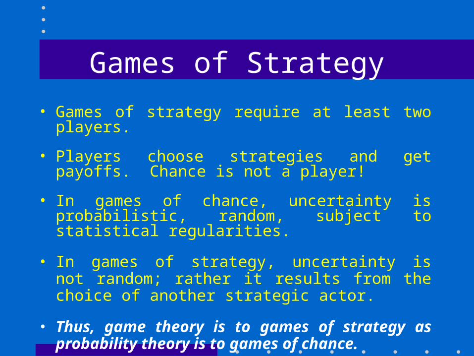
Games of Strategy

• Games of strategy require at least two players.

• Players choose strategies and get payoffs. Chance is not a player!

• In games of chance, uncertainty is probabilistic, random, subject to statistical regularities.

• In games of strategy, uncertainty is not random; rather it results from the choice of another strategic actor.

• Thus, game theory is to games of strategy as probability theory is to games of chance.

A Brief History of Game Theory

Minimax Theorem 1928

Theory of Games & Economic Behavior 1944

Nash Equilibrium 1950

Prisoner’s Dilemma 1950

The Evolution of Cooperation 1984

Nobel Prize: Harsanyi, Selten & Nash 1994

The Prisoner’s Dilemma

In years in jail Player 2

Confess Don’t

Confess

Player 1

Don’t

-10, -10 0, -20

-20, 0 -1, -1

The pair of dominant strategies (Confess, Confess)is a Nash Eq.

GAME 1.

The Prisoner’s Dilemma

Each player has a dominant strategy. Yet the outcome (-10, -10) is pareto inefficient.

Is this a result of imperfect information? What would happen if the players could communicate?

What would happen if the game were repeated? A finite number of times? An infinite or unknown number of times?

What would happen if rather than 2, there were many players?

DominanceDefinition

Dominant Strategy: a strategy that is best no matter what the opponent(s) choose(s).

T1 T2 T3 T1 T2 T3

0,2 4,3 3,3

4,0 5,4 5,6 3,5 3,5 2,3

0,2 4,3 3,3

4,0 5,4 5,3 3,5 3,5 2,3

S1

S2

S3

S1

S2

S3

Sure Thing Principle: If you have a dominant strategy, use it!

(S2,T3)(S2,T2)

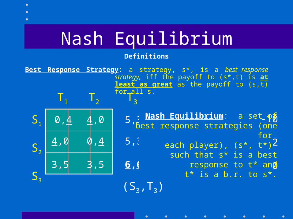
Nash EquilibriumDefinitions

Best Response Strategy: a strategy, s*, is a best response strategy, iff the payoff to (s*,t) is at least as great as the payoff to (s,t) for all s.

-3 0 -10

-1 5 2

-2 -4 0

0,4 4,0 5,3

4,0 0,4 5,3 3,5 3,5 6,6

S1

S2

S3

S1

S2

S3

T1 T2 T3

Nash Equilibrium: a set of best response strategies (one for

each player), (s*, t*) such that s* is a best

response to t* and t* is a b.r. to s*.

(S3,T3)

Nash Equilibrium

-3 0 -10

-1 5 2

-2 -4 0

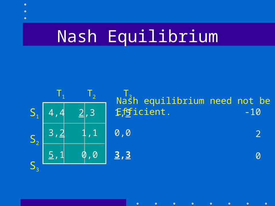
4,4 2,3 1,5

3,2 1,1 0,0 5,1 0,0 3,3

S1

S2

S3

S1

S2

S3

T1 T2 T3Nash equilibrium need not be Efficient.

Nash Equilibrium

-3 0 -10

-1 5 2

-2 -4 0

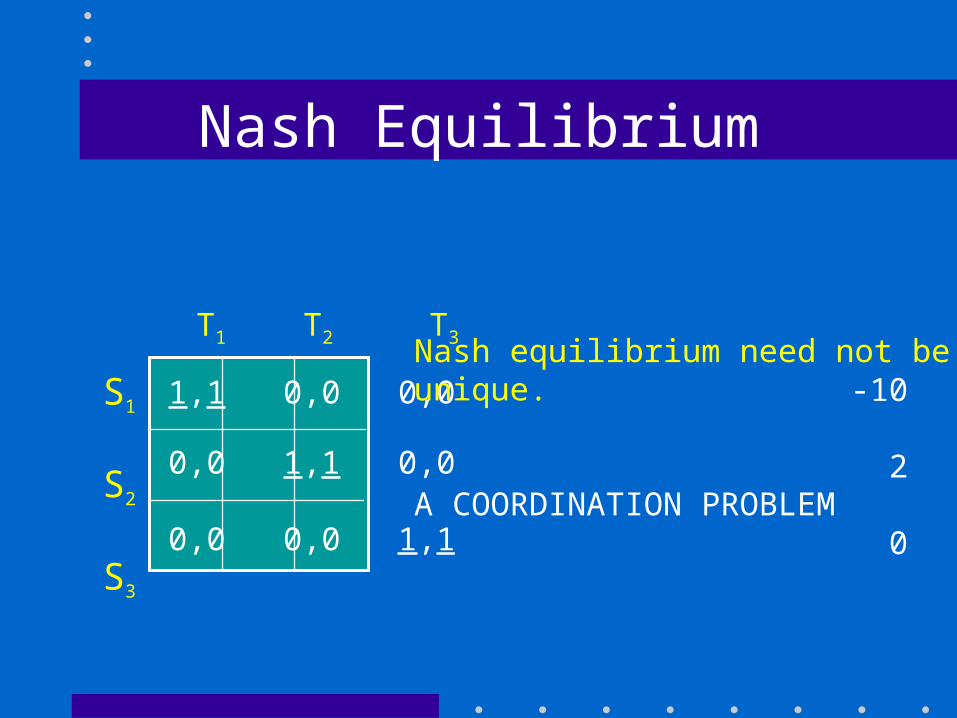
1,1 0,0 0,0

0,0 1,1 0,0 0,0 0,0 1,1

S1

S2

S3

S1

S2

S3

T1 T2 T3Nash equilibrium need not be unique.

A COORDINATION PROBLEM

Nash Equilibrium

-3 0 -10

-1 5 2

-2 -4 0

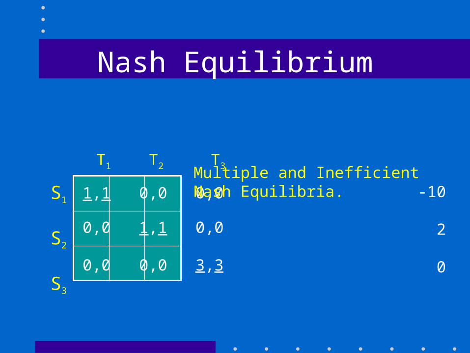
1,1 0,0 0,0

0,0 1,1 0,0 0,0 0,0 3,3

S1

S2

S3

S1

S2

S3

T1 T2 T3Multiple and Inefficient Nash Equilibria.

Nash Equilibrium

-3 0 -10

-1 5 2

-2 -4 0

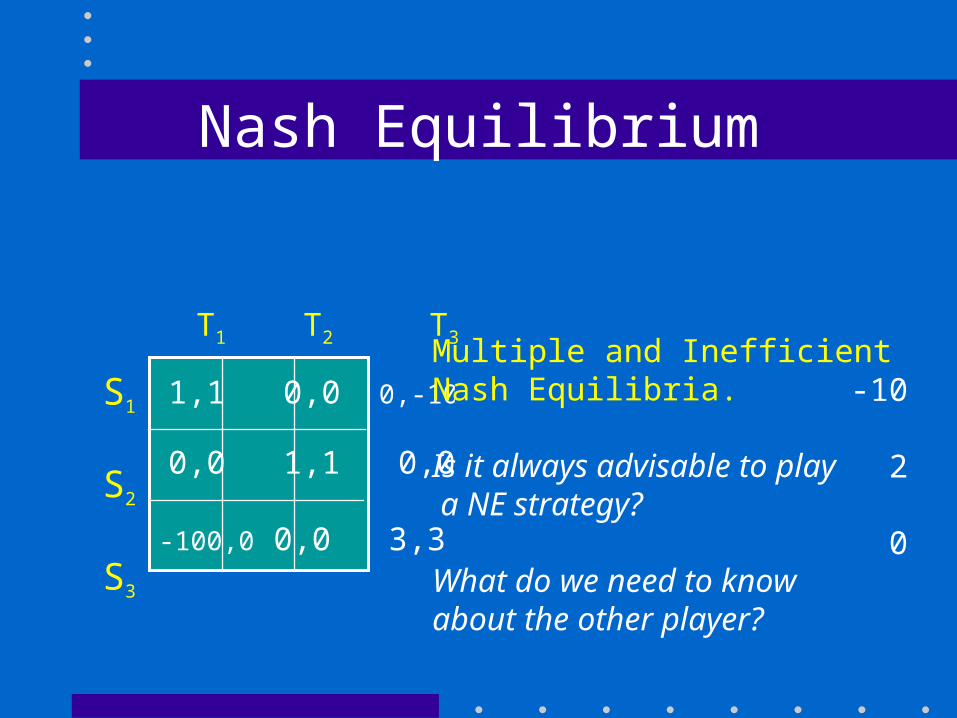
1,1 0,0 0,-100

0,0 1,1 0,0 -100,0 0,0 3,3

S1

S2

S3

S1

S2

S3

T1 T2 T3Multiple and Inefficient Nash Equilibria.

Is it always advisable to play a NE strategy?

What do we need to know about the other player?

Next Time

7/21 Strategic Competition

Pindyck and Rubenfeld, Ch 13.

Besanko, Ch. 14.