79

Power Transmission

Devices UNIT 3 POWER TRANSMISSION DEVICES

Structure

3.1 Introduction

Objectives

3.2 Power Transmission Devices

3.2.1 Belts

3.2.2 Chain

3.2.3 Gears

3.3 Transmission Screw

3.4 Power Transmission by Belts

3.4.1 Law of Belting

3.4.2 Length of the Belt

3.4.3 Cone Pulleys

3.4.4 Ratio of Tensions

3.4.5 Power Transmitted by Belt Drive

3.4.6 Tension due to Centrifugal Forces

3.4.7 Initial Tension

3.4.8 Maximum Power Transmitted

3.5 Kinematics of Chain Drive

3.6 Classification of Gears

3.6.1 Parallel Shafts

3.6.2 Intersecting Shafts

3.6.3 Skew Shafts

3.7 Gear Terminology

3.8 Gear Train

3.8.1 Simple Gear Train

3.8.2 Compound Gear Train

3.8.3 Power Transmitted by Simple Spur Gear

3.9 Summary

3.10 Key Words

3.11 Answers to SAQs

3.1 INTRODUCTION

The power is transmitted from one shaft to the other by means of belts, chains and gears.

The belts and ropes are flexible members which are used where distance between the

two shafts is large. The chains also have flexibility but they are preferred for

intermediate distances. The gears are used when the shafts are very close with each

other. This type of drive is also called positive drive because there is no slip. If the

distance is slightly larger, chain drive can be used for making it a positive drive. Belts

and ropes transmit power due to the friction between the belt or rope and the pulley.

There is a possibility of slip and creep and that is why, this drive is not a positive drive.

A gear train is a combination of gears which are used for transmitting motion from one

shaft to another.

80

Theory of Machines

Objectives

After studying this unit, you should be able to

understand power transmission derives,

understand law of belting,

determine power transmitted by belt drive and gear,

determine dimensions of belt for given power to be transmitted,

understand kinematics of chain drive,

determine gear ratio for different type of gear trains,

classify gears, and

understand gear terminology.

3.2 POWER TRANSMISSION DEVICES

Power transmission devices are very commonly used to transmit power from one shaft to

another. Belts, chains and gears are used for this purpose. When the distance between the

shafts is large, belts or ropes are used and for intermediate distance chains can be used.

For belt drive distance can be maximum but this should not be more than ten metres for

good results. Gear drive is used for short distances.

3.2.1 Belts

In case of belts, friction between the belt and pulley is used to transmit power. In

practice, there is always some amount of slip between belt and pulleys, therefore, exact

velocity ratio cannot be obtained. That is why, belt drive is not a positive drive.

Therefore, the belt drive is used where exact velocity ratio is not required.

The following types of belts shown in Figure 3.1 are most commonly used :

(a) Flat Belt and Pulley (b) V-belt and Pulley (c) Circular Belt or Rope Pulley

Figure 3.1 : Types of Belt and Pulley

The flat belt is rectangular in cross-section as shown in Figure 3.1(a). The pulley for this

belt is slightly crowned to prevent slip of the belt to one side. It utilises the friction

between the flat surface of the belt and pulley.

The V-belt is trapezoidal in section as shown in Figure 3.1(b). It utilizes the force of

friction between the inclined sides of the belt and pulley. They are preferred when

distance is comparative shorter. Several V-belts can also be used together if power

transmitted is more.

The circular belt or rope is circular in section as shown in Figure 8.1(c). Several ropes

also can be used together to transmit more power.

The belt drives are of the following types :

(a) open belt drive, and

(b) cross belt drive.

Open Belt Drive

Open belt drive is used when sense of rotation of both the pulleys is same. It is

desirable to keep the tight side of the belt on the lower side and slack side at the

81

Power Transmission

Devices top to increase the angle of contact on the pulleys. This type of drive is shown in

Figure 3.2.

Figure 3.2 : Open Belt Derive

Cross Belt Drive

In case of cross belt drive, the pulleys rotate in the opposite direction. The angle of

contact of belt on both the pulleys is equal. This drive is shown in Figure 3.3. As

shown in the figure, the belt has to bend in two different planes. As a result of this,

belt wears very fast and therefore, this type of drive is not preferred for power

transmission. This can be used for transmission of speed at low power.

Figure 3.3 : Cross Belt Drive

Since power transmitted by a belt drive is due to the friction, belt drive is

subjected to slip and creep.

Let d1 and d2 be the diameters of driving and driven pulleys, respectively. N1 and

N2 be the corresponding speeds of driving and driven pulleys, respectively.

The velocity of the belt passing over the driver

1 11

60

d NV

If there is no slip between the belt and pulley

2 21 2

60

d NV V

or, 1 1 2 2

60 60

d N d N

or, 1 2

2 1

N d

N d

If thickness of the belt is ‘t’, and it is not negligible in comparison to the diameter,

1 2

2 1

N d t

N d t

Let there be total percentage slip ‘S’ in the belt drive which can be taken into

account as follows :

2 1 1100

SV V

or 2 2 1 1 160 60 100

d N d N S

Driving Pulley

Slack Side Thickness

Effective Radius

Driving Pulley

Neutral Section

Tight Side

82

Theory of Machines

If the thickness of belt is also to be considered

or 1 2

2 1

( ) 1

( )1

100

N d t

SN d t

or, 2 1

1 2

( )1

( ) 100

N d t S

N d t

The belt moves from the tight side to the slack side and vice-versa, there is some

loss of power because the length of belt continuously extends on tight side and

contracts on loose side. Thus, there is relative motion between the belt and pulley

due to body slip. This is known as creep.

3.2.2 Chain

The belt drive is not a positive drive because of creep and slip. The chain drive is a

positive drive. Like belts, chains can be used for larger centre distances. They are made

of metal and due to this chain is heavier than the belt but they are flexible like belts. It

also requires lubrication from time to time. The lubricant prevents chain from rusting

and reduces wear.

The chain and chain drive are shown in Figure 3.4. The sprockets are used in place of

pulleys. The projected teeth of sprockets fit in the recesses of the chain. The distance

between roller centers of two adjacent links is known as pitch. The circle passing

through the pitch centers is called pitch circle.

(a) (b)

(c) (d)

Figure 3.4 : Chain and Chain Drive

Let ‘’ be the angle made by the pitch of the chain, and

‘r’ be the pitch circle radius, then

pitch, 2 sin2

p r

or, cosec2 2

pr

The power transmission chains are made of steel and hardened to reduce wear. These

chains are classified into three categories

(a) Block chain

(b) Roller chain

(c) Inverted tooth chain (silent chain)

Pin Pitch

Pitch

Roller Bushing

Sprocket

r

φ

p

83

Power Transmission

Devices Out of these three categories roller chain shown in Figure 3.4(b) is most commonly used.

The construction of this type of chain is shown in the figure. The roller is made of steel

and then hardened to reduce the wear. A good roller chain is quiter in operation as

compared to the block chain and it has lesser wear. The block chain is shown in

Figure 3.4(a). It is used for low speed drive. The inverted tooth chain is shown in

Figures 3.4(c) and (d). It is also called as silent chain because it runs very quietly even at

higher speeds.

3.2.3 Gears

Gears are also used for power transmission. This is accomplished by the successive

engagement of teeth. The two gears transmit motion by the direct contact like chain

drive. Gears also provide positive drive.

The drive between the two gears can be represented by using plain cylinders or discs 1

and 2 having diameters equal to their pitch circles as shown in Figure 3.5. The point of

contact of the two pitch surfaces shell have velocity along the common tangent. Because

there is no slip, definite motion of gear 1 can be transmitted to gear 2 or vice-versa.

The tangential velocity ‘Vp’ = 1 r1 = 2 r2

where r1 and r2 are pitch circle radii of gears 1 and 2, respectively.

Figure 3.5 : Gear Drive

or, 1 21 2

2 2

60 60

N Nr r

or, 1 1 2 2N r N r

or, 1 2

2 1

N r

N r

Since, pitch circle radius of a gear is proportional to its number of teeth (t).

1 2

2 1

N t

N t

where t1 and t2 are the number of teeth on gears 1 and 2, respectively.

SAQ 1

In which type of drive centre distance between the shafts is lowest? Give reason

for this?

3.3 TRANSMISSION SCREW

In a screw, teeth are cut around its circular periphery which form helical path. A nut has

similar internal helix in its bore. When nut is turned on the screw with a force applied

tangentially, screw moves forward. For one turn, movement is equal to one lead. In case

of lead screw, screw rotates and nut moves along the axis over which tool post is

mounted.

N1

N2

2 1

VP

84

Theory of Machines

Let dm be the mean diameter of the screw,

be angle of friction, and

p be the pitch.

If one helix is unwound, it will be similar to an inclined plane for which the angle of

inclination ‘’ is given by (Figure 3.6)

tan

L

dm

For single start L = p

tan

p

dm

If force acting along the axis of the screw is W, effort applied tangential to the screw

(as discussed in Unit 2)

tan ( ) P W

for motion against force.

Also tan ( ) P W

for motion in direction of force.

Figure 3.6 : Transmission Screw

3.3.1 Power Transmitted

Torque acting on the screw

tan ( )2 2

dm W dm

T P

If speed is N rpm

Power transmitted 2

watt60

T N

tan ( )

2 kW2 60 1000

W dmN

3.4 POWER TRANSMISSION BY BELTS

In this section, we shall discuss how power is transmitted by a belt drive. The belts are

used to transmit very small power to the high amount of power. In some cases magnitude

of the power is negligible but the transmission of speed only may be important. In such

cases the axes of the two shafts may not be parallel. In some cases to increase the angle

L = p

W

P

dm

85

Power Transmission

Devices of lap on the smaller pulley, the idler pulley is used. The angle of lap may be defined as

the angle of contact between the belt and the pulley. With the increase in angle of lap,

the belt drive can transmit more power. Along with the increase in angle of lap, the idler

pulley also does not allow reduction in the initial tension in the belt. The use of idler

pulley is shown in Figure 3.7.

Figure 3.7 : Use of Idler in Belt Drive

SAQ 2

(a) What is the main advantage of idler pulley?

(b) A prime mover drives a dc generator by belt drive. The speeds of prime

mover and generator are 300 rpm and 500 rpm, respectively. The diameter

of the driver pulley is 600 mm. The slip in the drive is 3%. Determine

diameter of the generator pulley if belt is 6 mm thick.

3.4.1 Law of Belting

The law of belting states that the centre line of the belt as it approaches the pulley, must

lie in plane perpendicular to the axis of the pulley in the mid plane of the pulley

otherwise the belt will run off the pulley. However, the point at which the belt leaves the

other pulley must lie in the plane of a pulley.

The Figure 3.8 below shows the belt drive in which two pulleys are at right angle to each

other. It can be seen that the centre line of the belt approaching larger or smaller pulley

lies in its plane. The point at which the belt leaves is contained in the plane of the other

pulley.

If motion of the belt is reversed, the law of the belting will be violated. Therefore,

motion is possible in one direction in case of non-parallel shafts as shown in Figure 3.8.

Figure 3.8 : Law of Belting

Idler Pulley

86

Theory of Machines

3.4.2 Length of the Belt

For any type of the belt drive it is always desirable to know the length of belt required. It

will be required in the selection of the belt. The length can be determined by the

geometric considerations. However, actual length is slightly shorter than the theoretically

determined value.

Open Belt Drive

The open belt drive is shown in Figure 3.9. Let O1 and O2 be the pulley centers

and AB and CD be the common tangents on the circles representing the two

pulleys. The total length of the belt ‘L’ is given by

L = AB + Arc BHD + DC + Arc CGA

Let r be the radius of the smaller pulley,

R be the radius of the larger pulley,

C be the centre distance between the pulleys, and

be the angle subtended by the tangents AB and CD with O1 O2.

Figure 3.9 : Open Belt Drive

Draw O1 N parallel to CD to meet O2 D at N.

By geometry, O2 O1, N = C O1 J = D O2 K=

Arc BHD = ( + 2) R,

Arc CGA = ( 2) r

AB = CD = O1 N = O1 O2 cos = C cos

sinR r

C

or, 1 ( )sin

R r

C

2 21cos 1 sin 1 sin

2

21( 2 ) ( 2 ) 2 1 sin

2L R r C

For small value of ; ( )R r

C

, the approximate lengths

2( ) 1

( ) 2 ( ) 2 12

R r R rL R r R r C

C C

22( ) 1( ) 2 1

2

R r R rR r C

C C

This provides approximate length because of the approximation taken earlier.

D K

C

A

B

G

C J

β = r

β

O1 O2 R

N

H β

87

Power Transmission

Devices Crossed-Belt Drive

The crossed-belt drive is shown in Figure 3.10. Draw O1 N parallel to the line CD

which meets extended O2 D at N. By geometry

1 2 2 1CO J DO K O O N

Arc ArcL AGC AB BKD CD

Arc ( 2 ), and Arc ( 2 )AGC r BKD R

1 ( )sin or sin

R r R r

C C

For small value of

R r

C

2

2 2

2

1 1 ( )cos 1 sin 1 sin 1

2 2

R r

C

( 2 ) 2 cos ( 2 )L r C R

( 2 ) ( ) 2 cosR r C

Figure 3.10 : Cross Belt Drive

For approximate length

2 2

2

( ) 1 ( )( ) 2 2 1

2

R r R rL R r C

C C

2( )

( ) 2R r

R r CC

SAQ 3

Which type of drive requires longer length for same centre distance and size of

pulleys?

3.4.3 Cone Pulleys

Sometimes the driving shaft is driven by the motor which rotates at constant speed but

the driven shaft is designed to be driven at different speeds. This can be easily done by

using stepped or cone pulleys as shown in Figure 3.11. The cone pulley has different sets

of radii and they are selected such that the same belt can be used at different sets of the

cone pulleys.

A

G

C J

β

r

D K

β

O1 O2

R

N

C

β

B

88

Theory of Machines

Figure 3.11 : Cone Pulleys

Let Nd be the speed of the driving shaft which is constant.

Nn be the speed of the driven shaft when the belt is on nth step.

rn be the radius of the nth step of driving pulley.

Rn be the radius of the nth step of the driven pulley.

where n is an integer, 1, 2, . . .

The speed ratio is inversely proportional to the pulley radii

1 1

1d

N r

N R . . . (3.1)

For this first step radii r1 and R1 can be chosen conveniently.

For second pair 2 2

2d

N r

N R , and similarly n n

d n

N r

N R .

In order to use same belt on all the steps, the length of the belt should be same

i.e. 1 2 . . . nL L L . . . (3.2)

Thus, two equations are available – one provided by the speed ratio and other provided

by the length relation and for selected speed ratio, the two radii can be calculated. Also it

has to be kept in mind that the two pulleys are same. It is desirable that the speed ratios

should be in geometric progression.

Let k be the ratio of progression of speed.

32

1 2 1

. . . n

n

N NNk

N N N

22 1 3 1andN k N N k N

1 1 11

1

n nn d

rN k N k N

R

232 1 1

2 1 3 1

and rr r r

k kR R R R

Since, both the pulleys are made similar.

1

r3

R3

2 3 4

5

89

Power Transmission

Devices 11 1 1

1 1 1

or nn

n

r R r Rk

R r R r

or, 11

1

nRk

r

. . . (3.3)

If radii R1 and r1 have been chosen, the above equations provides value of k or vice-

versa.

SAQ 4

How the speed ratios are selected for cone pulleys?

3.4.4 Ratio of Tensions

The belt drive is used to transmit power from one shaft to the another. Due to the friction

between the pulley and the belt one side of the belt becomes tight side and other

becomes slack side. We have to first determine ratio of tensions.

Flat Belt

Let tension on the tight side be ‘T1’ and the tension on the slack side be ‘T2’. Let

‘’ be the angle of lap and let ‘’ be the coefficient of friction between the belt

and the pulley. Consider an infinitesimal length of the belt PQ which subtend an

angle at the centre of the pulley. Let ‘R’ be the reaction between the element

and the pulley. Let ‘T’ be tension on the slack side of the element, i.e. at point P

and let ‘(T + T)’ be the tension on the tight side of the element.

The tensions T and (T + T) shall be acting tangential to the pulley and thereby

normal to the radii OP and OQ. The friction force shall be equal to ‘R’ and its

action will be to prevent slipping of the belt. The friction force will act

tangentially to the pulley at the point S.

Figure 3.12 : Ratio of Tensions in Flat Belt

Considering equilibrium of the element at S and equating it to zero.

Resolving all the forces in the tangential direction

cos ( ) cos 02 2

R T T T

or, cos2

R T

. . . (3.4)

T + ST

R

R

S

Q

P

δ θ

O

T2

T

T1

θ

δ θ 2

δ θ

2

90

Theory of Machines

Resolving all the forces in the radial direction at S and equating it to zero.

sin ( ) sin 02 2

R T T T

or, (2 ) sin2

R T T

Since is very small, taking limits

cos 1 and sin2 2 2

(2 )2 2

R T T T T

Neglecting the product of the two infinitesimal quantities 2

T

which is

negligible in comparison to other quantities :

R T

Substituting the value of R and cos 12

in Eq. (3.4), we get

T T

or, T

T

Taking limits on both sides as 0

dT

dT

Integrating between limits, it becomes

1

2 0

T

T

dTd

T

or, 1

2

lnT

T

or, 1

2

Te

T

. . . (3.5)

V-belt or Rope

The V-belt or rope makes contact on the two sides of the groove as shown in

Figure 3.13.

(a) (b)

Figure 3.13 : Ratio of Tension in V-Belt

T + δ T

2 Rn sinα

S

Q

δ θ/2

2μ Rn P

O

T2

T

T1

θ

δ θ/2

α

2α Rn

α

Rn

91

Power Transmission

Devices Let the reaction be ‘Rn’ on each of the two sides of the groove. The resultant

reaction will be 2Rn sin at point S.

Resolving all the forces tangentially in the Figure 3.13(b), we get

2 cos ( ) cos 02 2

nR T T T

or, 2 cos2

nR T

. . . (3.6)

Resolving all the forces radially, we get

2 sin sin ( ) sin2 2

nR T T T

(2 ) sin2

T T

Since is very small

sin2 2

2 sin (2 )2 2

nR T T T T

Neglecting the product of the two infinitesimal quantities

2 sinnR T

or, 2sin

n

TR

Substituting the value of Rn and using the approximation cos 12

, in Eq. (3.6),

we get

sin

TT

or, sin

T

T

Taking the limits and integrating between limits, we get

1

2 0sin

T

T

dTd

T

or, 1

2

lnsin

T

T

or, sin1

2

T

eT

. . . (3.7)

SAQ 5

(a) If a rope makes two full turn and one quarter turn how much will be angle

of lap?

(b) If smaller pulley has coefficient of friction 0.3 and larger pulley has

coefficient of friction 0.2. The angle of lap on smaller and larger pulleys are

160o and 200

o which value of () should be used for ratio of tensions?

92

Theory of Machines

3.4.5 Power Transmitted by Belt Drive

The power transmitted by the belt depends on the tension on the two sides and the belt

speed.

Let T1 be the tension on the tight side in ‘N’

T2 be the tension on the slack side in ‘N’, and

V be the speed of the belt in m/sec.

Then power transmitted by the belt is given by

Power 1 2( ) WattP T T V

1 2( )kW

1000

T T V . . . (3.8)

or,

21

1

1

kW1000

TT V

TP

If belt is on the point of slipping.

1

2

Te

T

1 (1 )kW

1000

T e VP

. . . (3.9)

The maximum tension T1 depends on the capacity of the belt to withstand force. If

allowable stress in the belt is ‘t’ in ‘Pa’, i.e. N/m2, then

1 ( ) NtT t b . . . (3.10)

where t is thickness of the belt in ‘m’ and b is width of the belt also in m.

The above equations can also be used to determine ‘b’ for given power and speed.

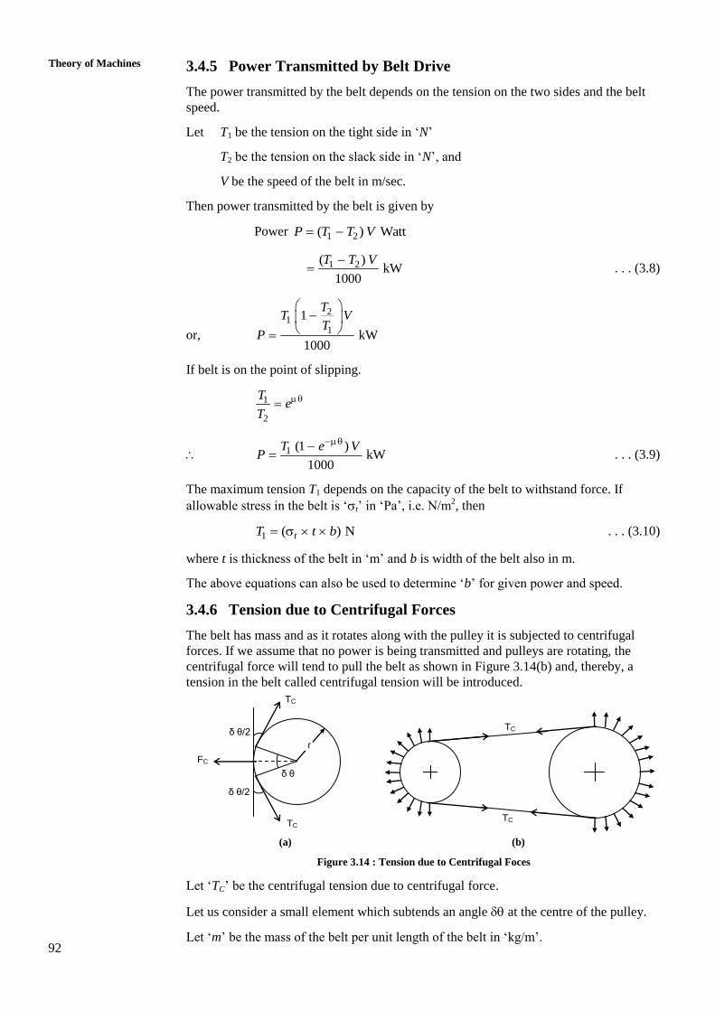
3.4.6 Tension due to Centrifugal Forces

The belt has mass and as it rotates along with the pulley it is subjected to centrifugal

forces. If we assume that no power is being transmitted and pulleys are rotating, the

centrifugal force will tend to pull the belt as shown in Figure 3.14(b) and, thereby, a

tension in the belt called centrifugal tension will be introduced.

(a) (b)

Figure 3.14 : Tension due to Centrifugal Foces

Let ‘TC’ be the centrifugal tension due to centrifugal force.

Let us consider a small element which subtends an angle at the centre of the pulley.

Let ‘m’ be the mass of the belt per unit length of the belt in ‘kg/m’.

TC

TC

δ θ/2

r

δ θ/2

FC

TC

TC

δ θ

93

Power Transmission

Devices The centrifugal force ‘Fc’ on the element will be given by

2

( )C

VF r m

r

where V is speed of the belt in m/sec. and r is the radius of pulley in ‘m’.

Resolving the forces on the element normal to the tangent

2 sin 02

C CF T

Since is very small.

sin2 2

or, 2 02

C CF T

or, C CF T

Substituting for FC

2

C

m Vr T

r

or, 2CT m V . . . (3.11)

Therefore, considering the effect of the centrifugal tension, the belt tension on the tight

side when power is transmitted is given by

Tension of tight side 1t CT T T and tension on the slack side 2s CT T T .

The centrifugal tension has an effect on the power transmitted because maximum tension

can be only Tt which is

t tT t b

21 tT t b m V

SAQ 6

What will be the centrifugal tension if mass of belt is zero?

3.4.7 Initial Tension

When a belt is mounted on the pulley some amount of initial tension say ‘T0’ is provided

in the belt, otherwise power transmission is not possible because a loose belt cannot

sustain difference in the tension and no power can be transmitted.

When the drive is stationary the total tension on both sides will be ‘2 T0’.

When belt drive is transmitting power the total tension on both sides will be (T1 + T2),

where T1 is tension on tight side, and T2 is tension on the slack side.

If effect of centrifugal tension is neglected.

0 1 22T T T

94

Theory of Machines

or, 1 20

2

T TT

If effect of centrifugal tension is considered, then

0 1 2 2t s CT T T T T T

or, 1 20

2C

T TT T

. . . (3.12)

3.4.8 Maximum Power Transmitted

The power transmitted depends on the tension ‘T1’, angle of lap , coefficient of friction

‘’ and belt speed ‘V’. For a given belt drive, the maximum tension (Tt), angle of lap and

coefficient of friction shall remain constant provided that

(a) the tension on tight side, i.e. maximum tension should be equal to the

maximum permissible value for the belt, and

(b) the belt should be on the point of slipping.

Therefore, Power 1 (1 )P T e V

Since, 1 t cT T T

or, ( ) (1 )t cP T T e V

or, 2( ) (1 )tP T m V e V

For maximum power transmitted

2( 3 ) (1 )t

dPT m V e

dV

or, 23 0tT m V

or, 3 0 t cT T

or, 3

tc

TT

or, 2

3 tT

m V

Also, 3

tTV

m . . . (3.13)

At the belt speed given by the Eq. (3.13) the power transmitted by the belt drive shall be

maximum.

SAQ 7

What is the value of centrifugal tension corresponding to the maximum power

transmitted?

95

Power Transmission

Devices 3.5 KINEMATICS OF CHAIN DRIVE

The chain is wrapped round the sprocket as shown in Figure 3.4(d). The chain in motion

is shown in Figure 3.15. It may be observed that the position of axial line changes

between the two position as shown by the dotted line and full line. The dotted line meets

at point B when extended with the line of centers. The firm line meets the line of centers

at point A when extended. The speed of the driving sprocket say ‘1’ shall be constant

but the velocity of chain will vary between 1 O1 C and 1 O1 D. Therefore,

2 1

1 2

O A

O B

Figure 3.15 : Kinematics of Chain Drive

The variation in the chain speed causes the variation in the angular speed of the driven

sprocket. The angular speed of the driven sprocket will vary between

1 11 1

2 2

andO B O A

O B O A

This variation can be reduced by increasing number of teeth on the sprocket.

3.6 CLASSIFICATION OF GEARS

There are different types of arrangement of shafts which are used in practice. According

to the relative positions of shaft axes, different types of gears are used.

3.6.1 Parallel Shafts

In this arrangement, the shaft axes lie in parallel planes and remain parallel to one

another. The following type of gears are used on these shafts :

Spur Gears

These gears have straight teeth with their alignment parallel to the axes. These

gears are shown in mesh in Figures 3.16(a) and (b). The contact between the two

meshing teeth is along a line whose length is equal to entire length of teeth. It may

be observed that in external meshing, the two shafts rotate opposite to each other

whereas in internal meshing the shafts rotate in the same sense.

(a) External Meshing (b) Internal Meshing

Figure 3.16 : Spur Gears

If the gears mesh externally and diameter of one gear becomes infinite, the

arrangement becomes ‘Spur Rack and Pinion’. This is shown in Figure 3.17. It

converts rotary motion into translatory motion, or vice-versa.

ώ1 ώ2

o1 o2

D

C

A B

Line Contact

Line Contact

96

Theory of Machines

Figure 3.17 : Spur Rack and Pinion

Helical Gears or Helical Spur Gears

In helical gears, the teeth make an angle with the axes of the gears which is called

helix angle. The two meshing gears have same helix angle but its layout is in

opposite sense as shown in Figure 3.18.

Figure 3.18 : Helical Gears

The contact between two teeth occurs at a point of the leading edge. The point

moves along a diagonal line across the teeth. This results in gradual transfer of

load and reduction in impact load and thereby reduction in noise. Unlike spur

gears the helical gears introduce thrust along the axis of the shaft which is to be

borne by thrust bearings.

Double-Helical or Herringbone Gears

A double-helical gear is equivalent to a pair of helical gears having equal helix

angle secured together, one having a right-hand helix and the other a left-hand

helix. The teeth of two rows are separated by a groove which is required for tool

run out. The axial thrust which occurs in case of single-helical gears is eliminated

in double helical gears. If the left and right inclinations of a double helical gear

meet at a common apex and groove is eliminated in it, the gear is known as

herringbone gear as shown in Figure 3.19.

Figure 3.19 : Herringbone Gears

Line Contact

Drivern Thrust

Thrust

Driver

97

Power Transmission

Devices 3.6.2 Intersecting Shafts

The motion between two intersecting shafts is equivalent to rolling of two conical

frustums from kinematical point of view.

Straight Bevel Gears

These gears have straight teeth which are radial to the point of intersection of the

shaft axes. Their teeth vary in cross section through out their length. Generally,

they are used to connect shafts at right angles. These gears are shown in

Figure 3.20. The teeth make line contact like spur gears.

Figure 3.20 : Straight Bevel Gears

As a special case, gears of the same size and connecting two shafts at right angle

to each other are known as mitre gears.

Spiral Bevel Gears

When the teeth of a bevel gear are inclined at an angle to the face of the bevel,

these gears are known as spiral bevel gears or helical bevel gears. A gear of this

type is shown in Figure 3.21(a). They run quiter in action and have point contact.

If spiral bevel gear has curved teeth but with zero degree spiral angle, it is known

as zerol bevel gear.

(a) Spiral Bevel Gear (b) Zerol Bevel Gear

Figure 3.21 : Spiral Bevel Gears

3.6.3 Skew Shafts

These shafts are non-parallel and non-intersecting. The motion of the two mating gears is

equivalent to motion of two hyperboloids in contact as shown in Figure 3.22. The angle

between the two shafts is equal to the sum of the angles of the two hyperboloids. That is

1 2

The minimum perpendicular distance between the two shafts is equal to the sum of the

throat radii.

Figure 3.22 : Hyperboloids in Contact

Ψ2

Ψ1

θ B

1 2

A Line of contact

98

Theory of Machines

Crossed-Helical Gears or Spiral Gears

They can be used for any two shafts at any angle as shown in Figure 3.23 by a

suitable choice of helix angle. These gears are used to drive feed mechanisms on

machine tool.

Figure 3.23 : Spiral Gears in Contact

Worm Gears

It is a special case of spiral gears in which angle between the two axes is generally

right angle. The smaller of the two gears is called worm which has large spiral

angle. These are shown in Figure 3.24.

(a) (b)

(c) (d)

Figure 3.24 : Worm Gears

Hypoid Gears

These gears are approximations of hyperboloids though look like spiral bevel

gears. The hypoid pinion is larger and stronger than a spiral bevel pinion. They

have quit and smooth action and have larger number of teeth is contact as

compared to straight bevel gears. These gears are used in final drive of vehicles.

They are shown in Figure 3.25.

Figure 3.25 : Hypoid Gears

1

2

99

Power Transmission

Devices 3.7 GEAR TERMINOLOGY

Before considering kinematics of gears we shall define the terms used for describing the

shape, size and geometry of a gear tooth. The definitions given here are with respect to a

straight spur gear.

Pitch Circle or Pitch Curve

It is the theoretical curve along which the gear rolls without slipping on the

corresponding pitch curve of other gear for transmitting equivalent motion.

Pitch Point

It is the point of contact of two pitch circles.

Pinion

It is the smaller of the two mating gears. It is usually the driving gear.

Rack

It is type of the gear which has infinite pitch circle diameter.

Circular Pitch

It is the distance along the pitch circle circumference between the corresponding

points on the consecutive teeth. It is shown in Figure 3.26.

Figure 3.26 : Gear Terminology

If d is diameter of the pitch circle and ‘T’ be number of teeth, the circular pitch

(pc) is given by

c

dp

T

. . . (3.14)

Diamental Pitch

It is defined as the number of teeth per unit pitch circle diameter. Therefore,

diamental pitch (pd) can be expressed as

d

Tp

d . . . (3.15)

From Eqs. (3.14) and (3.15)

cd

dp

T p

d

or, c dp p . . . (3.16)

Circular Pitch

Top Land

Face

Flank

Addendumm

Working Depth

Clearance

Dedendum Bottom Land

Dedendum (Root) Circle

Pitch Circle

Addendum Circle

Face Width

Space Width

Tooth Thicknes

s

100

Theory of Machines

Module

It is the ratio of the pitch circle diameter to the number of teeth. Therefore, the

module (m) can be expressed as

d

mT

. . . (3.17)

From Eqs. (8.14)

cp m . . . (3.18)

Addendum Circle and Addendum

It is the circle passing through the tips of gear teeth and addendum is the radial

distance between pitch circle and the addendum circle.

Dedendum Circle and Dedendum

It is the circle passing through the roots of the teeth and the dedendum is the radial

distance between root circle and pitch circle.

Full Depth of Teeth and Working Depth

Full depth is sum of addendum and dedendum and working depth is sum of

addendums of the two gears which are in mesh.

Tooth Thickness and Space Width

Tooth thickness is the thickness of tooth measured along the pitch circle and space

width is the space between two consecutive teeth measured along the pitch circle.

They are equal to each other and measure half of circular pitch.

Top Land and Bottom Land

Top land is the top surface of the tooth and the bottom land is the bottom surface

between the adjacent fillets.

Face and Flank

Tooth surface between the pitch surface and the top land is called face whereas

flank is tooth surface between pitch surface and the bottom land.

Pressure Line and Pressure Angle

The driving tooth exerts a force on the driven tooth along the common normal.

This line is called pressure line. The angle between the pressure line and the

common tangent to the pitch circles is known as pressure angle.

Path of Contact

The path of contact is the locus of a point of contact of two mating teeth from the

beginning of engagement to the end of engagement.

Arc of Approach and Arc of Recess

Arc of approach is the locus of a point on the pitch circle from the beginning of

engagement to the pitch point. The arc of recess is the locus of a point from pitch

point upto the end of engagement of two mating gears.

Arc of Contact

It is the locus of a point on the pitch circle from the beginning of engagement to

the end of engagement of two mating gears.

Arc of Contact = Arc of Approach + Arc of Recess

Angle of Action

It is the angle turned by a gear from beginning of engagement to the end of

engagement of a pair of teeth.

Angle of action = Angle turned during arc of approach + Angle turned during arc

of recess

101

Power Transmission

Devices Contact Ratio

It is equal to the number of teeth in contact and it is the ratio of arc of contact to

the circular pitch. It is also equal to the ratio of angle of action to pitch angle.

Figure 3.27 : Gear Terminology

3.8 GEAR TRAIN

A gear train is combination of gears that is used for transmitting motion from one shaft

to another.

There are several types of gear trains. In some cases, the axes of rotation of the gears are

fixed in space. In one case, gears revolve about axes which are not fixed in space.

3.8.1 Simple Gear Train

In this gear train, there are series of gears which are capable of receiving and

transmitting motion from one gear to another. They may mesh externally or internally.

Each gear rotates about separate axis fixed to the frame. Figure 3.28 shows two gears in

external meshing and internal meshing.

Let t1, t2 be number of teeth on gears 1 and 2.

(a) External Meshing (b) Internal Meshing

Figure 3.28 : Simple Gear Train

B

Dedendum Circle

Path of Contact

Drivers

Ψ Pressure Angle

Pitch Circle

Base Circle

Dedendum Circle

Angle of Action

F

P

C

E

A

D

Pitch Circle

+

1 2

+

1

2

P

102

Theory of Machines

Let N1, N2 be speed in rpm for gears 1 and 2. The velocity of P,

1 1 2 22 2

60 60

P

N d N dV

1 2 2

2 1 1

N d t

N d t

Referring Figure 3.28, the two meshing gears in external meshing rotate in opposite

sense whereas in internal meshing they rotate in same sense. In simple gear train, there

can be more than two gears also as shown in Figure 3.29.

Figure 3.29 : Gear Train

Let N1, N2, N3, . . . be speed in rpm of gears 1, 2, 3, . . . etc., and t1, t2, t3, . . . be number

of teeth of respective gears 1, 2, 3, . . . , etc.

In this gear train, gear 1 is input gear, gear 4 is output gear and gears 2, 3 are

intermediate gears. The gear ratio of the gear train is give by

Gear Ratio 31 1 2

4 2 3 4

NN N N

N N N N

3 31 2 2 4

2 1 3 2 4 3

; andt NN t N t

N t N t N t

Therefore, 31 2 4 4

4 1 2 3 1

tN t t t

N t t t t

This expression indicates that the intermediate gears have no effect on gear ratio. These

intermediate gears fill the space between input and output gears and have effect on the

sense of rotation of output gear.

SAQ 8

(a) There are six gears meshing externally and input gear is rotating in

clockwise sense. Determine sense of rotation of the output gear.

(b) Determine sense of rotation of output gear in relation to input gear if a

simple gear train has four gears in which gears 2 and 3 mesh internally

whereas other gears have external meshing.

3.8.2 Compound Gear Train

In this type of gear train, at least two gears are mounted on the same shaft and they rotate

at the same speed. This gear train is shown in Figure 3.30 where gears 2 and 3 are

mounted on same shaft and they rotate at the same speed, i.e.

2 3N N

1 2

3

4

103

Power Transmission

Devices

Figure 3.30 : Compound Gear Train

Let N1, N2, N3, . . . be speed in rpm of gears 1, 2, 3, . . . , etc. and t1, t2, t3, . . . , etc. be

number of teeth of respective gears 1, 2, 3, . . . , etc.

Gear Ratio 31 1 2 1

4 2 4 2 4

NN N N N

N N N N N

2 4

1 3

t t

t t

Therefore, unlike simple gear train the gear ratio is contributed by all the gears. This

gear train is used in conventional automobile gear box.

Conventional Automobile Gear Box

A conventional gear box of an automobile uses compound gear train. For different

gear engagement, it may use sliding mesh arrangement, constant mesh

arrangement or synchromesh arrangement. Discussion of these arrangements is

beyond the scope of this course. We shall restrict ourselves to the gear train. It can

be explained better with the help of an example.

Example 3.1

A sliding mesh type gear box with four forward speeds has following gear ratios :

Top gear = 1

Third gear = 1.38

Second gear = 2.24

First gear = 4

Determine number of teeth on various gears. The minimum number of teeth on the

pinion should not be less than 18. The gear box should have minimum size and

variation in the ratios should be as small as possible.

Solution

The gears in the gear box are shown in Figure 3.31 below :

Figure 3.31 : Conventional Gear Box

1

2 4

3

A

B

C

E

G

D F

H

Dog Clutch

Engine Shaft Input Shaft

Main Splined Shaft

(Output Shaft)

Lay Shaft

104

Theory of Machines

For providing first gear ratio, gear A meshes with gear B and gear H meshes with

gear G.

Speed of engine shaftFirst gear ratio =

Speed of output shaft

A A H A H

G H G B G

N N N N N

N N N N N

[i.e. NB = NH]

GB

A H

tt

t t

For smallest size of gear box GB

A H

tt

t t

4.0 2.0GB

A H

tt

t t

If tA = 20 teeth tH = 20

tB = 2 20 = 40 teeth and tG = 20 2 = 40 teeth

Since centre distance should be same

A B C D E F H Gt t t t t t t t

40 20 60C Dt t . . . (3.19)

60E Ft t . . . (3.20)

For second gear, gear A meshes with gear B and gear E meshes with gear F.

2.24A

G

N

N

or, 2.24A F

B E

N N

N N

2.24B E

A F

t t

t t

or, 2 2.24F

G

t

t

or, 2.24

1.122

E

F

t

t . . . (3.21)

From Eqs. (10.2) and (10.3)

1.12 60F Ft t

or, 60

28.3 602.12

F E Ft t t

or, 60 28.3 31.7Et

Since number of teeth have to be in full number. Therefore, tF can be either 28 or

29 and tE can be either 31 or 32. If tF = 28 and tE = 32.

Second gear ratio 40 32

2.28620 28

A E

B F

t t

t t

105

Power Transmission

Devices If tF = 29 and tE = 31.

Second gear ratio 40 31

2.13820 29

From these two values of gear ratios, 2.286 is closer to 2.24 than 2.138.

For third gear, gear A meshes with gear B and gear D meshes with gear C.

1.38A

C

N

N

or, 1.38A D

B C

N N

N N

or, 1.38CB

A D

tt

t t

or, 40

1.3820

C

D

t

t

2 1.38C

D

t

t

or, 1.38

0.692

C

D

t

t . . . (3.22)

From Eqs. (3.19) and (3.20)

tC = 0.69 tD

tD + 0.69 tD = 60

or, 60

35.5031.69

Dt

60 60.35.503 24.497 C Dt t

Either tC = 24 and tD = 36 or tC = 25 and tD = 35.

If tC = 25 and tD = 35.

Third gear ratio 40 25

1.428620 35

CB

A D

tt

t t

If tC = 24 and tD = 36

Third gear ratio 40 24

1.33320 36

Since 1.333 is closer to 1.38 as compared to 1.4286.

Therefore, tC = 24 and tD = 36

The top gear requires direct connection between input shaft and output shaft.

3.8.3 Power Transmitted by Simple Spur Gear

When power is bring transmitted by a spur gear, tooth load Fn acts normal to the profile.

It can be resolved into two components Fn cos and Fn sin . Fn cos acts tangentially

to the pitch circle and it is responsible for transmission of power

Power transmitted (P) = Fn cos . V

where V is pitch line velocity.

106

Theory of Machines

Since 2

60 2

N tmV

2

cos60 2

n

N tmP F

where t is number of teeth and m is module.

Figure 3.32

Example 3.2

An open flat belt drive is required to transmit 20 kW. The diameter of one of the

pulleys is 150 cm having speed equal to 300 rpm. The minimum angle of contact

may be taken as 170o. The permissible stress in the belt may be taken as

300 N/cm2. The coefficient of friction between belt and pulley surface is 0.3.

Determine

(a) width of the belt neglecting effect of centrifugal tension for belt

thickness equal to 8 mm.

(b) width of belt considering the effect of centrifugal tension for the

thickness equal to that in (a). The density of the belt material

is 1.0 gm/cm3.

Solution

Given that Power transmitted (p) = 20 kW

Diameter of pulley (d) = 150 cm = 1.5 m

Speed of the belt (N) = 300 rpm

Angle of lap () o 170170 2.387 radian

180

Coefficient of friction () = 0.3

Permissible stress () = 300 N/cm2

(a) Thickness of the belt (t) = 8 mm = 0.8 cm

Let higher tension be ‘T1’ and lower tension be ‘T2’.

0.3 2.3871

2

2.53T

e eT

The maximum tension ‘T1’ is controlled by the permissible stress.

Fn

Pressure

angle

107

Power Transmission

Devices 1 300 0.8 24 N10

bT b t b

Here b is in mm

Therefore, 12

24N

2.53 2.53

T bT

Velocity of belt 2 2 300 1.5

23.5 m/s60 2 60 2

N dV

Power transmitted 1 2

24 23.5( ) 24 kW

2.53 1000

bp T T V b

1 23.5 347.3

24 12.53 1000 1000

bb

Since P = 20 kW

347.3

201000

b

or, 20 1000

36.4 mm347.3

b

(b) The density of the belt material = 1 gm/cm3

Mass of the belt material/length, m = b t 1 metre

210.8 100 0.8 10 kg/m

1000 10

b

b

38 10 kg/mb

Centrifugal tension ‘TC’ = m V2

or, 3 28 10 (23.5) = 4.418 NCT b b

Maximum tension (Tmax) = 24b N

1 max 24 4.418 19.58CT T T b b b

Power transmitted 1

11P T V

e

1 23.5 460.177

19.58 12.53 1000 1000

bb

Also P = 20 kW

460.177

201000

b

or, b = 45.4 mm

The effect of the centrifugal tension increases the width of the belt required.

Example 3.3

An open belt drive is required to transmit 15 kW from a motor running at 740 rpm.

The diameter of the motor pulley is 30 cm. The driven pulley runs at 300 rpm and

is mounted on a shaft which is 3 metres away from the driving shaft. Density of

the leather belt is 0.1 gm/cm3. Allowable stress for the belt material is 250 N/cm

2.

If coefficient of friction between the belt and pulley is 0.3, determine width of the

belt required. The thickness of the belt is 9.75 mm.

108

Theory of Machines

Solution

Given data :

Power transmitted (P) = 15 kW

Speed of motor pulley (N1) = 740 rpm

Diameter of motor pulley (d1) = 30 cm

Speed of driven pulley (N2) = 300 rpm

Distance between shaft axes (C) = 3 m

Density of the belt material () = 0.1 gm/cm3

Allowable stress () = 250 N/cm2

Coefficient of friction () = 0.3

Let the diameter of the driven pulley be ‘d2’

N1 d1 = N2 d2

1 12

2

740 3074 cm

300

N dd

N

12 1 74 30sin sin

2 2 300

d d

C

or, = 0.0734 radian

2 2.94 rad

Mass of belt ‘m’ = b t one metre length

0.1 9.75

1001000 10 10

b

where ‘b’ is width of the belt in ‘mm’

or, 30.975 10 kg/mm b

max

9.75250 24.375 N

10 10

bT b

Active tension ‘T’ = Tmax – TC

Velocity of belt 1 12

60 2

N dV

740 30

60 100

or, V = 11.62 m/s

2 3 20.975 10 (11.62)CT m V b

= 0.132 b N

1 24.375 0.132 24.243T b b b

Power transmitted 1

11P T V

e

109

Power Transmission

Devices 0.3 2.94 2.47e e

1 11.62 165

24.243 12.47 1000 1000

bP

165

15 or 91 mm100

bb

Example 3.4

An open belt drive has two pulleys having diameters 1.2 m and 0.5 m. The pulley

shafts are parallel to each other with axes 4 m apart. The mass of the belt is 1 kg

per metre length. The tension is not allowed to exceed 2000 N. The larger pulley

is driving pulley and it rotates at 200 rpm. Speed of the driven pulley is 450 rpm

due to the belt slip. The coefficient of the friction is 0.3. Determine

(a) power transmitted,

(b) power lost in friction, and

(c) efficiency of the drive.

Solution

Data given :

Diameter of driver pulley (d1) = 1.2 m

Diameter of driven pulley (d2) = 0.5 m

Centre distance (C) = 4 m

Mass of belt (m) = 1 kg/m

Maximum tension (Tmax) = 2000 N

Speed of driver pulley (N1) = 200 rpm

Speed of driven pulley (N2) = 450 rpm

Coefficient of friction () = 0.3

(a) 11

2 2 20020.93 r/s

60 60

N

22

2 2 45047.1 r/s

60 60

N

Velocity of the belt (V) 1.2

20.93 12.56 m/s2

Centrifugal tension (TC) = m V2 = 1 (12.56)

2 = 157.75 N

Active tension on tight side (T1) = Tmax – TC

or, T1 = 2000 – 157.75 = 1842.25 N

1 2 1.2 0.5sin 0.0875

2 2 4

d d

C

or, = 5.015o

o180 2 180 2 5.015 169.985

or,

169.9850.3

1 180

2

2.43T

e eT

110

Theory of Machines

Power transmitted 1

1( ) 1 12.56

2.43P T

1 12.56

1842.25 1 kW2.43 1000

= 13.67 kW

(b) Power output 2 21

11 W

2.43 2

dT

1 47.1 0.5

1842.25 1 12.2 kW2.43 2 1000

Power lost in friction = 13.67 – 12.2 = 1.47 kW

(c) Efficiency of the drive Power transmitted 12.2

0.89 or 89%Power input 13.67

.

Example 3.5

A leather belt is mounted on two pulleys. The larger pulley has diameter equal to

1.2 m and rotates at speed equal to 25 rad/s. The angle of lap is 150o. The

maximum permissible tension in the belt is 1200 N. The coefficient of friction

between the belt and pulley is 0.25. Determine the maximum power which can be

transmitted by the belt if initial tension in the belt lies between 800 N and 960 N.

Solution

Given data :

Diameter of larger pulley (d1) = 1.2 m

Speed of larger pulley 1 = 25 rad/s

Speed of smaller pulley 2 = 50 rad/s

Angle of lap () = 150o

Initial tension (T0) = 800 to 960 N

Let the effect of centrifugal tension be negligible.

The maximum tension (T1) = 1200 N

1500.25

1 180

2

1.924T

e eT

12

1200623.6 N

1.924 1.924

TT

1 20

1200 623.6911.8 N

2 2

T TT

Maximum power transmitted (Pmax) = (T1 – T2) V

Velocity of belt (V) 11

1.225

2 2

d

V = 15 m/s

max (1200 623.6) (1200 623.6) 15P V

8646 W or 8.646 kW

111

Power Transmission

Devices Example 3.6

A shaft carries pulley of 100 cm diameter which rotates at 500 rpm. The ropes

drive another pulley with a speed reduction of 2 : 1. The drive transmits 190 kW.

The groove angle is 40o. The distance between pulley centers is 2.0 m. The

coefficient of friction between ropes and pulley is 0.20. The rope weighs

0.12 kg/m. The allowable stress for the rope is 175 N/cm2. The initial tension in

the rope is limited to 800 N. Determine :

(a) number of ropes and rope diameter, and

(b) length of each rope.

Solution

Given data :

Diameter of driving pulley (d1) = 100 cm = 1 m

Speed of the driving pulley (N1) = 500 rpm

Speed of the driven pulley (N2) = 250 rpm

Power transmitted (P) = 190 kW

Groove angle () = 40o

Centre distance (C) = 2 m

Coefficient of friction () = 0.2

Mass of rope = 0.12 kg/m

Allowable stress () = 175 N/cm2

Initial tension (T0) = 800 N

The velocity of rope 1 1 1 50026.18 m/s

60 60

d N

Centrifugal tension (TC) = 0.12 (26.18)2 = 82.25 N

2 1( ) 2 1sin 0.25

2 2 2

d d

C

or, = sin 0.25– 1

= 14.18

Angle of lap () = 2 = 151o or 2.636 radian

o

0.2 2.636

sin 201

2

4.67T

eT

or, T1 = 4.67 T2

Initial tension (T0) 1 2 2

8002

CT T T

1 2 1600 2 82.25 1600 164.5 1435.5 NT T

2 24.67 1435.5T T

or, T2 = 253.1 N

T1 = 4.67 T2 = 1182.0 N

1 2

26.18( ) (1182.0 253.1) 24.32 kW

1000 1000

VP T T

Numbers of ropes required (n) 190

7.8124.32

or say 8 ropes,

112

Theory of Machines

Maximum tension (Tmax) = T1 + TC

= 1182 + 82.25 = 1264.25 N

2max 1264.25

4T d

or, 2 1264.25 49.2

175d

or, d = 3.03 cm

This is open belt drive, therefore, formula for length of rope is given by

22( ) 1( ) 2 1

2

R r R rL R r C

C C

2 12 11 m, 0.5 m

2 2 2 2

d dR r

22(1 0.5) 1 1 0.5(1 0.5) 2 2 1

2 2 2L

0.25

1.5 4 (1 0.5 0.0625) 8.72 m2

.

3.9 SUMMARY

The power transmission devices are belt drive, chain drive and gear drive. The belt drive

is used when distance between the shaft axes is large and there is no effect of slip on

power transmission. Chain drive is used for intermediate distance. Gear drive is used for

short centre distance. The gear drive and chain drive are positive drives but they are

comparatively costlier than belt drive.

Similarly, belt drive should satisfy law of belting otherwise it will slip to the side and

drive cannot be performed. When belt drive transmits power, one side will become tight

side and other side will become loose side. The ratio of tension depends on the angle of

lap and coefficient of friction. If coefficient of friction is same on both the pulleys

smaller angle of lap will be used in the formula. If coefficient of friction is different, the

minimum value of product of coefficient of friction and angle of lap will decide the ratio

of tension, i.e. power transmitted. Due to the mass of belt, centrifugal tension acts and

reduces power transmitted. For a given belt drive the power transmitted will be

maximum at a speed for which centrifugal tension is one third of maximum possible

tension.

The gears can be classified according to the layout of their shafts. For parallel shafts spur

or helical gears are used and bevel gears are uded for intersecting shafts. For skew shafts

when angle between the axes is 90o worm and worm gears are used. When distance

between the axes of shaft is larger and positive drive is required, chain drive is used. We

can see the use of chain drive in case of tanks, motorcycles, etc.

3.10 KEY WORDS

Spur Gears : They have straight teeth with teeth layout is

parallel to the axis of shaft.

Helical Gears : They have curved or straight teeth and its

inclination with shaft axis is called helix angle.

113

Power Transmission

Devices Herringbone Gears : It is a double helical gear having left and right

inclinations which meet at a common apex and

there is no groove in between them.

Bevel Gear : They have teeth radial to the point of intersection

of the shaft axes and they vary in cross-section

throughout their length.

Spiral Gears : They have curved teeth which are inclined to the

shaft axis. They are used for skew shafts.

Worm Gears : It is special case of spiral gears where angle

between axes of skew shafts is 90o.

Rack and Pinion : Rack is special case of a spur gear whose pitch

circle diameter is infinite and it meshes with a

pinion.

Hypoid Gears : These gears are approximations of hyperboloids

but they look like spiral gears.

Pitch Cylinders : A pair of gears in mesh can be replaced by a pair

of imaginary friction cylinders which by pure

rolling motion transmit the same motion as pair of

gears.

Pitch Diameter : It is diameter of pitch cylinders.

Circular Pitch : It is the distance between corresponding points of

the consecutive teeth along pitch cylinder.

Diametral Pitch : It is the ratio of number of teeth to the diameter of

the pitch cylinders.

Module : It is the ratio of diameter of pitch cylinder to the

number of teeth.

Addendum : It is the radial height of tooth above pitch cylinder.

Dedendum : It is the radial depth of tooth below pitch cylinder.

Pressure Angle : It is the angle between common tangent to the two

pitch cylinders and common normal at the point of

contact between teeth (pressure line).

3.11 ANSWERS TO SAQs

SAQ 1

Available in text.

SAQ 2

(a) Available in text.

(b) Available in text.

SAQ 3

(a) Available in text.

(b) Data given :

Speed of prime mover (N1) = 300 rpm

Speed of generator (N2) = 500 rpm

Diameter of driver pulley (d1) = 600 mm

Slip in the drive (s) = 3%

Thickness of belt (t) = 6 mm

114

Theory of Machines

If there is no slip 2 1

1 2

N d

N d .

If thickness of belt is appreciable and no slip

2 1

1 2

N d t

N d t

If thickness of belt is appreciable and slip is ‘S’ in the drive

2 1

1 2

1100

N d t S

N d t

2

500 600 6 31

300 100d t

or, 2

606( 6) 300 0.97 352.692

500d

or, 2 352.692 6 346.692 mmd

SAQ 4

Available in text.

SAQ 5

Available in text.

SAQ 6

Available in text.

SAQ 7

Available in text.

SAQ 8

Available in text.

137

Governors

UNIT 5 GOVERNORS

Structure

5.1 Introduction

Objectives

5.2 Classification of Governors

5.3 Gravity Controlled Centrifugal Governors

5.3.1 Watt Governor

5.3.2 Porter Governor

5.4 Spring Controlled Centrifugal Governors

5.5 Governor Effort and Power

5.6 Characteristics of Governors

5.7 Controlling Force and Stability of Spring Controlled Governors

5.8 Insensitiveness in the Governors

5.9 Summary

5.10 Key Words

5.11 Answers to SAQs

5.1 INTRODUCTION

In the last unit, you studied flywheel which minimises fluctuations of speed within the

cycle but it cannot minimise fluctuations due to load variation. This means flywheel does

not exercise any control over mean speed of the engine. To minimise fluctuations in the

mean speed which may occur due to load variation, governor is used. The governor has

no influence over cyclic speed fluctuations but it controls the mean speed over a long

period during which load on the engine may vary.

When there is change in load, variation in speed also takes place then governor operates

a regulatory control and adjusts the fuel supply to maintain the mean speed nearly

constant. Therefore, the governor automatically regulates through linkages, the energy

supply to the engine as demanded by variation of load so that the engine speed is

maintained nearly constant.

Figure 5.1 shows an illustrative sketch of a governor along with linkages which regulates

the supply to the engine. The governor shaft is rotated by the engine. If load on the

engine increases the engine speed tends to reduce, as a result of which governor balls

move inwards. This causes sleeve to move downwards and this movement is transmitted

to the valve through linkages to increase the opening and, thereby, to increase the supply.

On the other hand, reduction in the load increases engine speed. As a result of which the

governor balls try to fly outwards. This causes an upward movement of the sleeve and it

reduces the supply. Thus, the energy input (fuel supply in IC engines, steam in steam

turbines, water in hydraulic turbines) is adjusted to the new load on the engine. Thus the

governor senses the change in speed and then regulates the supply. Due to this type of

action it is simple example of a mechanical feedback control system which senses the

output and regulates input accordingly.

138

Theory of Machines

Figure 5.1 : Governor and Linkages

Objectives

After studying this unit, you should be able to

classify governors,

analyse different type of governors,

know characteristics of governors,

know stability of spring controlled governors, and

compare different type of governors.

5.2 CLASSIFICATION OF GOVERNORS

The broad classification of governor can be made depending on their operation.

(a) Centrifugal governors

(b) Inertia and flywheel governors

(c) Pickering governors.

Centrifugal Governors

In these governors, the change in centrifugal forces of the rotating masses due to

change in the speed of the engine is utilised for movement of the governor sleeve.

One of this type of governors is shown in Figure 5.1. These governors are

commonly used because of simplicity in operation.

Inertia and Flywheel Governors

In these governors, the inertia forces caused by the angular acceleration of the

engine shaft or flywheel by change in speed are utilised for the movement of the

balls. The movement of the balls is due to the rate of change of speed in stead of

change in speed itself as in case of centrifugal governors. Thus, these governors

are more sensitive than centrifugal governors.

Pickering Governors

This type of governor is used for driving a gramophone. As compared to the

centrifugal governors, the sleeve movement is very small. It controls the speed by

dissipating the excess kinetic energy. It is very simple in construction and can be

used for a small machine.

FC

mg mg

FC

Bell Crank Lener

Engine Pulley

Supply

pip

e

139

Governors 5.2.1 Types of Centrifugal Governors

Depending on the construction these governors are of two types :

(a) Gravity controlled centrifugal governors, and

(b) Spring controlled centrifugal governors.

Gravity Controlled Centrifugal Governors

In this type of governors there is gravity force due to weight on the sleeve or

weight of sleeve itself which controls movement of the sleeve. These governors

are comparatively larger in size.

Spring Controlled Centrifugal Governors

In these governors, a helical spring or several springs are utilised to control the

movement of sleeve or balls. These governors are comparatively smaller in size.

SAQ 1

(a) Compare flywheel with governor.

(b) Which type of control the governor system is?

(c) Compare centrifugal governors with inertia governors.

5.3 GRAVITY CONTROLLED CENTRIFUGAL

GOVERNORS

There are three commonly used gravity controlled centrifugal governors :

(a) Watt governor

(b) Porter governor

(c) Proell governor

Watt governor does not carry dead weight at the sleeve. Porter governor and proell

governor have heavy dead weight at the sleeve. In porter governor balls are placed at the

junction of upper and lower arms. In case of proell governor the balls are placed at the

extension of lower arms. The sensitiveness of watt governor is poor at high speed and

this limits its field of application. Porter governor is more sensitive than watt governor.

The proell governor is most sensitive out of these three.

5.3.1 Watt Governor

This governor was used by James Watt in his steam engine. The spindle is driven by the

output shaft of the prime mover. The balls are mounted at the junction of the two arms.

The upper arms are connected to the spindle and lower arms are connected to the sleeve

as shown in Figure 5.2(a).

(a) (b)

Figure 5.2 : Watt Governor

Ball Ball

Sleeve

h

mg FC

T

140

Theory of Machines

We ignore mass of the sleeve, upper and lower arms for simplicity of analysis. We can

ignore the friction also. The ball is subjected to the three forces which are centrifugal

force (Fc), weight (mg) and tension by upper arm (T). Taking moment about point O

(intersection of arm and spindle axis), we get

0CF h mg r

Since, 2CF mr

2 0mr h mg r

or 2 g

h . . . (5.1)

2

60

N

2 2 2

3600 894.56

4

gh

N N

. . . (5.2)

where ‘N’ is in rpm.

Figure 5.3 shows a graph between height ‘h’ and speed ‘N’ in rpm. At high speed the

change in height h is very small which indicates that the sensitiveness of the governor is

very poor at high speeds because of flatness of the curve at higher speeds.

Figure 5.3 : Graph between Height and Speed

SAQ 2

Why watt governor is very rarely used? Give reasons.

5.3.2 Porter Governor

A schematic diagram of the porter governor is shown in Figure 5.4(a). There are two sets

of arms. The top arms OA and OB connect balls to the hinge O. The hinge may be on the

spindle or slightly away. The lower arms support dead weight and connect balls also. All

of them rotate with the spindle. We can consider one-half of governor for equilibrium.

0.2

0.4

0.6

0.8

0.6

300 400 500 600 700

h

N

141

Governors Let w be the weight of the ball,

T1 and T2 be tension in upper and lower arms, respectively,

Fc be the centrifugal force,

r be the radius of rotation of the ball from axis, and

I is the instantaneous centre of the lower arm.

Taking moment of all forces acting on the ball about I and neglecting friction at the

sleeve, we get

02

C

WF AD w ID IC

or 2

C

wID W ID DCF

AD AD

or tan (tan tan )2

C

WF w

2C

wF r

g

2 tantan 1 1

2 tan

w Wr w

g w

or 2 tan 1 (1 )2

g WK

r w

. . . (5.3)

where tan

tanK

tanr

h

2 1 (1 )2

g WK

h w

. . . (5.4)

(a) (b)

Figure 5.4 : Porter Governor

If friction at the sleeve is f, the force at the sleeve should be replaced by W + f for rising

and by (W – f) for falling speed as friction apposes the motion of sleeve. Therefore, if the

friction at the sleeve is to be considered, W should be replaced by (W f). The

expression in Eq. (5.4) becomes

Arms

Spindle

Ball T1

T1

O

h

FC A

A

T2

r

T2 w

I D

A B

Central Load (w)

Sleeve C

Links

W

2 C

O

142

Theory of Machines

2 ( )1 (1 )

2

g W fK

h w

. . . (5.5)

SAQ 3

In which respect Porter governor is better than Watt governor?

5.4 SPRING CONTROLLED CENTRIFUGAL

GOVERNORS

In these governors springs are used to counteract the centrifugal force. They can be

designed to operate at high speeds. They are comparatively smaller in size. Their speed

range can be changed by changing the initial setting of the spring. They can work with

inclined axis of rotation also. These governors may be very suitable for IC engines, etc.

The most commonly used spring controlled centrifugal governors are :

(a) Hartnell governor

(b) Wilson-Hartnell governor

(c) Hartung governor

5.4.1 Hartnell Governor

The Hartnell governor is shown in Figure 5.5. The two bell crank levers have been

provided which can have rotating motion about fulcrums O and O. One end of each bell

crank lever carries a ball and a roller at the end of other arm. The rollers make contact

with the sleeve. The frame is connected to the spindle. A helical spring is mounted

around the spindle between frame and sleeve. With the rotation of the spindle, all these

parts rotate.

With the increase of speed, the radius of rotation of the balls increases and the rollers lift

the sleeve against the spring force. With the decrease in speed, the sleeve moves

downwards. The movement of the sleeve are transferred to the throttle of the engine

through linkages.

Figure 5.5 : Hartnell Governor

A

a

Fulcrum b

Roller

Spindle

O’

Collar

Bell crank Lever

Ball

Spring

Frame

Sleeve

O

Ball

c

143

Governors Let r1 = Minimum radius of rotation of ball centre from spindle axis, in m,

r2 = Maximum radius of rotation of ball centre from spindle axis, in m,

S1 = Spring force exerted on sleeve at minimum radius, in N,

S2 = Spring force exerted on sleeve at maximum radius, in N,

m = Mass of each ball, in kg,

M = Mass of sleeve, in kg,

N1 = Minimum speed of governor at minimum radius, in rpm,

N2 = Maximum speed of governor at maximum radius, in rpm,

1 and 2 = Corresponding minimum and maximum angular velocities, in r/s,

(FC)1 = Centrifugal force corresponding to minimum speed 21 1m r ,

(FC)2 = Centrifugal force corresponding to maximum speed 22 2m r ,

s = Stiffness of spring or the force required to compress the spring by one m,

r = Distance of fulcrum O from the governor axis or radius of rotation,

a = Length of ball arm of bell-crank lever, i.e. distance OA, and

b = Length of sleeve arm of bell-crank lever, i.e. distance OC.

Considering the position of the ball at radius ‘r1’, as shown in Figure 5.6(a) and taking

moments of all the forces about O

10 1 1 1 1

( )( ) cos sin cos 0

2C

Mg SM F a mg a b

or 11 1

( )( ) tan

2C

Mg S bF mg

a

. . . (5.9)

(a) (b)

Figure 5.6

Considering the position of the ball at radius ‘r2’ as shown in Figure 5.6(b) and taking

the moments of all the forces about O

20 2 2 2 2

( )( ) cos sin cos

2C

Mg SM F a mg a b

or 22 2

( )( ) tan

2C

Mg S bF mg

a

. . . (5.10)

r1

A1

mg (FC)1

r

1

1 x1

C1

(Mg + S1)

2

O

A’1

2 x2

C2

(Mg + S2)

2

r2

(FC)2

mg

A’2

A2

O’

C’2

C’1

Reaction at fulcrum

2

a

b

144

Theory of Machines

If 1 and 2 are very small and mass of the ball is negligible as compared to the spring

force, the terms 1tanmg and 2tanmg may be ignored.

11

( )( )

2C

Mg S bF

a

. . . (5.11)

and 22

( )( )

2C

Mg S bF

a

. . . (5.12)

2 12 1

( )( ) ( )

2C C

S S bF F

a

Total lift 1 2 1 2( ) ( )x x b b

1 2( )b

1 22 1

( ) ( )( )

r r r r bb r r

a a a

2 1 2 1Total lift ( )b

S S s r r sa

22 1

2 1

( )( ) ( )

2C C

r rbF F s

a

or stiffness of spring ‘s’

22 1

2 1

( ) ( )2

( )

C CF Fa

b r r

. . . (5.13)

For ball radius ‘r’

2 21 2 1

1 2 1

( ) ( ) ( )2 2

( )

C C C CF F F Fa as

b r r b r r

11 2 1

2 1

( )( ) {( ) ( ) }

( )C C C C

r rF F F F

r r

. . . (5.14)

SAQ 4

For IC engines, which type of governor you will prefer whether dead weight type

or spring controlled type? Give reasons.

5.5 GOVERNOR EFFORT AND POWER

Governor effort and power can be used to compare the effectiveness of different type of

governors.

Governor Effort

It is defined as the mean force exerted on the sleeve during a given change in

speed.

When governor speed is constant the net force at the sleeve is zero. When

governor speed increases, there will be a net force on the sleeve to move it

upwards and sleeve starts moving to the new equilibrium position where net force

becomes zero.

145

Governors Governor Power

It is defined as the work done at the sleeve for a given change in speed. Therefore,

Power of governor = Governor effort Displacement of sleeve

5.5.1 Determination of Governor Effort and Power

The effort and power of a Porter governor has been determined. The same principle can

be used for any other type of governor also.

(a) (b)

Figure 5.7

Figure 5.7 shows the two positions of a Porter governor.

Let N = Equilibrium speed corresponding to configuration shown in Figure 5.7(a),

W = Weight of sleeve in N,

h = Height of governor corresponding to speed N, and

c = A factor which when multiplied to equilibrium speed, gives the increase

in speed.

Increased speed = Equilibrium speed + Increase of speed,

= N + c . N = (1 + c) N, and . . . (5.15)

h1 = Height of governor corresponding to increased speed (1 + c ) N.

The equilibrium position of the governor for the increased speed is shown in

Figure 5.7(b). In order to prevent the sleeve from rising when the increase of speed takes

place, a downward force will have to be exerted on the sleeve.

Let W1 = New weight of sleeve so that the rising of sleeve is prevented when the speed is

(1 + c) N. This means that W1 is the weight of sleeve when height of governor

is h.

Downward force to be applied when the rising of sleeve is to be prevented when

speed increases from N to (1 + c) N = W1 – W.

When speed is N rpm and let the angles and are equal so that K = 1, the height h is

given by equation

2

2

60

w W gh

w N

. . . (5.16)

If the speed increases to (1 + c) N and height remains the same by increasing the load on

sleeve

1

22 (1 )

60

w W gh

w c N

. . . (5.17)

w

O

h

mg

h1

O

x

146

Theory of Machines

Equating the two values of h given by above equations, we get

12

{( )}

(1 )

w Ww W

c

21( ) (1 )w W c w W

21 ( ) (1 )W w W c w

21( ) ( ) (1 ) ( )W W w W c w W

2( ) {(1 ) 1}w W c

2 ( )c w W If c is very small . . . (5.18)

But W1 – W is the downward force which must be applied in order to prevent the sleeve

from rising when the increase of speed takes place. This is also the force exerted by the

governor on the sleeve when the speed changes from N to (1 + c) N. As the sleeve rises

to the new equilibrium position as shown in Figure 5.7(b), this force gradually

diminishes to zero. The mean force P exerted on the sleeve during the change of speed

from N to (1 + c) N is therefore given by

1 ( )2

W WP c w W

. . . (5.19)

This is the governor effort.

If weight on the sleeve is not increased

1 22 (1 )

60

w W gh

w c N

. . . (5.20)

1 2h h x

2

1

(1 )h

ch

2

1

1 (1 ) 1 2h

c ch

or 1

1

2h h

ch

or 1

22

xc

h

or 1x c h

Governor power 21 ( )Px c h w W . . . . (5.21)

5.6 CHARACTERISTICS OF GOVERNORS

Different governors can be compared on the basis of following characteristics :

Stability

A governor is said to be stable when there is one radius of rotation of the balls for

each speed which is within the speed range of the governor.

147

Governors Sensitiveness

The sensitiveness can be defined under the two situations :

(a) When the governor is considered as a single entity.

(b) When the governor is fitted in the prime mover and it is treated as

part of prime mover.

(a) A governor is said to be sensitive when there is larger displacement of the

sleeve due to a fractional change in speed. Smaller the change in speed of

the governor for a given displacement of the sleeve, the governor will be

more sensitive.

Sensitiveness 1 2

N

N N

. . . (5.22)

(b) The smaller the change in speed from no load to the full load, the more

sensitive the governor will be. According to this definition, the

sensitiveness of the governor shall be determined by the ratio of speed range

to the mean speed. The smaller the ratio more sensitive the governor will be

Sensitiveness 2 1 2 1

2 1

2( )

( )

N N N N

N N N

. . . (5.23)

where N2 – N1 = Speed range from no load to full load.

Isochronism

A governor is said to be isochronous if equilibrium speed is constant for all the

radii of rotation in the working range. Therefore, for an isochronous governor the

speed range is zero and this type of governor shall maintain constant speed.

Hunting

Whenever there is change in speed due to the change in load on the engine, the

sleeve moves towards the new position but because of inertia if overshoots the

desired position. Sleeve then moves back but again overshoots the desired position

due to inertia. This results in setting up of oscillations in engine speed. If the

frequency of fluctuations in engine speed coincides with the natural frequency of

oscillations of the governor, this results in increase of amplitude of oscillations

due to resonance. The governor, then, tends to intensity the speed variation instead

of controlling it. This phenomenon is known as hunting of the governor. Higher

the sensitiveness of the governor, the problem of hunting becomes more acute.

5.7 CONTROLLING FORCE AND STABILITY OF

SPRING CONTROLLED GOVERNORS

The resultant external force which controls the movement of the ball and acts along the

radial line towards the axis is called controlling force. This force acts at the centre of the

ball. It is equal and acts opposite to the direction of centrifugal force.

The controlling force ‘F’ = m 2 r.

Or

22

60

F Nm

r

For controlling force diagram in which ‘F’ is plotted against radius ‘r’, F

r represents

slope of the curve.

i.e. 2tanF

Nr . . . (5.24)

Therefore, for a stable governor slope in controlling force diagram should increase with

the increase in speed.

148

Theory of Machines

Stability of Spring-controlled Governors

Figure 5.8 shows the controlling force curves for stable, isochronous and unstable

spring controlled governors. The controlling force curve is approximately straight

line for spring controlled governors. As controlling force curve represents the

variation of controlling force ‘F’ with radius of rotation ‘r’, hence, straight line

equation can be,

; orF ar b F ar F ar b . . . (5.25)

where a and b are constants. In the above equation b may be +ve, or –ve or zero.

Figure 5.8 : Stability of Spring Controlled Governors

These three cases are as follows :

(a) We know that for a stable governor, the ratio F

r must increase as r

increases. Hence the controlling force curve DE for a stable governor

must intersect the controlling force axis (i.e. y-axis) below the origin,

when produced. Then the equation of the curve will be of the form

. orF b

F a r b ar r

. . . (5.26)

As r increases F

r increase and thereby tan increases. Therefore,

this equation represents stable governor.

(b) If b in the above equation is zero then the controlling force curve OC

will pass through the origin. The ratio F

r will be constant for all

radius of rotation and hence the governor will become isochronous.

Hence for isochronous, the equation will be

or constantF

F ar ar

. . . (5.27)

(c) If b is positive, then controlling force curve AB will intersect the

controlling force axis (i.e. y-axis) above the origin. The equation of

the curve will be

orF b

F ar b ar r

. . . (5.28)

As r increases, speed increases, F

r or tan reduces. Hence this

equation cannot represent stable governor but unstable governor.

Radius of Rotation D

Contr

olli

ng F

orc

e

O

A

B

C

E

Unstable F = ar + b

Isochronous F = ar

Stable F = ar – b

149

Governors 5.8 INSENSITIVENESS IN THE GOVERNORS

The friction force at the sleeve gives rise to the insensitiveness in the governor. At any

given radius there will be two different speeds one being when sleeve moves up and

other when sleeve moves down. Figure 5.9 shows the controlling force diagram for such

a governor.

Figure 5.9 : Insensitiveness in the Governors

The corresponding three values of speeds for the same radius OA are :

(a) The speed N when there is no friction.

(b) The speed N when speed is increasing or sleeve is on the verge of moving

up, and

(c) The speed N when speed is decreasing or sleeve on the verge of moving

down.

This means that, when radius is OA, the speed of rotation may vary between the limits

N and N, without causing any displacement of the governor sleeve. The governor is

said to be insensitive over this range of speed. Therefore,

Coefficient of insensitiveness N N

N

. . . (5.29)

Example 5.1

The arms of a Porter governor are 25 cm long and pivoted on the governor axis.

The mass of each ball is 5 kg and mass on central load of the sleeve is 30 kg. The

radius of rotation of balls is 15 cm when the sleeve begins to rise and reaches a

value of 20 cm for the maximum speed. Determine speed range.

Solution

Given data : Ball weight ‘w’ = 5 g N

Central load ‘W’ = 30 g N

Arm length ‘l’ = 25 cm = 0.25 m

Minimum radius ‘r1’ = 15 cm = 0.15 m

Maximum radius ‘r2’ = 20 cm = 0.2 m

Height 1

2 2 2 21' ' 0.25 0.15 0.2 mh l r

For k = 1.

c

B

D

A

Contr

olli

ng F

orc

e

Radius of Rotation

O

N’

N

N”

Speed Decreasing

Speed Increasing

Speed S

cale

150

Theory of Machines

Figure 5.10 : Figure for Example 5.1

Substituting values in Eq. (5.4)

21 1 (1 1)

0.2 2

g W

w

9.81 30

10.2 5

g

g

1 118.5297 r/s or 176.9 rpmN

Height 2 22 0.25 0.2 0.15 mh

22

9.81 301

0.15 5

g

g

2 229.396 r/s or 204.32 rpm N

Speed range = N2 – N1 = 204.32 – 176.9 = 27.42 rpm.

Example 5.2

In a Hartnell governor the radius of rotation is 7 cm when speed is 500 rpm. At

this speed, ball arm is normal and sleeve is at mid position. The sleeve movement

is 2 cm with 5% of change in speed. The mass of sleeve is 6 kg and friction is

equivalent to 25 N at the sleeve. The mass of the ball is 2 kg. If ball arm and

sleeve arms are equal, find,

(a) Spring rate,

(b) Initial compression in the spring, and

(c) Governor effort and power for 1% change in the speed if there is no

friction.

Solution

Sleeve mass ‘M’ = 6 kg

Friction force ‘f’ = 25 N

Ball mass ‘m’ = 2 kg

a b

Minimum radius r1 = 7 cm – 1 = 6 cm

Maximum radius r2 = 7 cm + 1 = 8 cm

2 500

52.36 r/s60

Maximum speed = 10.05 = 1.05 52.36 = 54.98 r/s

Minimum speed = 0.95 = 0.95 52.36 = 49.74 r/s

Neglecting the effect of obliquity of arms.

Fc

W l

l

r

h

w 2

151

Governors

(a) (b)

Figure 5.11 : Figure for Example 5.2

At Minimum Radius

1 1

112

2

C C

Mg S fF a b or F Mg S f

21 1 1 cF m r

212 (49.74) 0.06 2 6 25g S

1593.78 58.86 25S

Or 1 559.92S N

At Maximum Radius

2 22 CF Mg S f

22 2 2 cF m r

222 (54.98) 0.08 2 6 25g S

Or 2 883.44S N

Stiffness ‘s’ 2 1S S

x

883.44 559.92

0.02

Or 16175.81 N/ms

Initial compression 1

559.92

16175.81S

= 0.035 m or 3.5 cm

Governor Effort and Power

2

2C

Mg S fF

Increased speed = 1.01 = 1.01 52.36 = 52.88 r/s

At r = 0.07; 2 2 (52.36)2 0.07 = 6 g + S

At increased speed, 2 2 (52.88)2 0.07 = 6 g + 2 P + S

where P is governor effort.

1

mg

6 cm

FC

,

O

1 cm

Mg + S1

2

Mg + S2

2

2

2 O

8 cm

Fc2

F

1 cm mg

152

Theory of Machines

2 22 2 2 0.07 {(52.88) (52.36) }P

Or P = 7.66 N

Let the spring force corresponding to speed 52.88 r/s be S.

22 2 (52.88) 0.07 6g S

2 2( ) 2 2 0.07 {(52.88) (52.36) }S S

= 15.32 N

Sleeve lift for 1% change 15.32

s

415.329.47 10 m

16175.81

Governor power 47.66 9.47 10

37.25 10 Nm

Example 5.3

The controlling force diagram of a spring controlled governor is a straight line.

The weight of each governor ball is 40 N. The extreme radii of rotation of balls

are 10 cm and 17.5 cm. The corresponding controlling forces at these radii are

205 N and 400 N. Determine :

(a) the extreme equilibrium speeds of the governor, and

(b) the equilibrium speed and the coefficient of insensitivenss at a radius

of 15 cm. The friction of the mechanism is equivalent of 2.5 N at each

ball.

Solution

Weight of each ball ‘w’ = 40 N

r1 = 10 cm and r2 = 17.5 cm

1 2205 N and 400 NC CF F

Let CF ar b

when 11 10 cm 0.1 m and 205 NCr F

205 = b + 0.1 a

when 22 17.5 cm 0.175 m and 400 NCr F

400 = b + 0.175 a

195 0.075 2600a a

205 0.1 2600 55b

55 2600CF r

(a) For

21240

205; 0.1 205 N60

C

NF

g

Or 1 214.1 rpmN

For FC = 400; r = 0.175 m

22240

0.175 40060

N

g

Or 2 226.1 rpmN

153

Governors (b) FC = k N2

At radius r = 15 cm

2C bF f k N

2C bF f k N

2 2( ) ( ) ( )C b C bF f F f k N N

Or 2 ( ) ( )bf k N N N N

2 ( )k N N N

2

2 2 ( ) 2 ( )b

C

f k N N N N N

F Nk N

Coefficient of insensitiveness 2( ) 1

2

b b

C C

f fN N

N F F

At r = 0.15 m

55 2600 0.15 335 NCF

Coefficient of insensitiveness 32.57.46 10

335

Or 0.746%.

5.9 SUMMARY

The governors are control mechanisms and they work on the principle of feedback

control. Their basic function is to control the speed within limits when the load on the

prime mover changes. They have no control over the change is speed within the cycle.

The speed control within the cycle is done by the flywheel.

The governors are classified in three main categories that is centrifugal governors,

inertial governor and pickering governor. The use of the two later governors is very

limited and in most of the cases centrifugal governors are used. The centrifugal

governors are classified into two main categories, gravity controlled type and spring

loaded type.

The gravity controlled type of governors are larger in size and require more space as

compared to the spring controlled governors. This type of governors are two, i.e. Porter

governor and Proell governor. The spring controlled governors are : Hartnel governor,

Wilson-Hartnell governor and Hartung governor.

For comparing different type of governors, effort and power is used. They determine

whether a particular type of governor is suitable for a given situation or not. To

categorise a governor the characteristics can be used. It can be determined whether a

governor is stable or isochronous or it is prone to hunting. The friction at the sleeve

gives rise to the insensitiveness in the governor. At any particular radius, there shall be

two speeds due to the friction. Therefore, it is most desirable that the friction should be

as low as possible.

The stability of a spring controlled governor can be determined by drawing controlling

force diagram which should have intercept on the negative side of Y-axis.

5.10 KEY WORDS

Watt Governor : It is a type of governor which does not have load

on the sleeve.

Porter Governor : This is a type of governor which has dead weight

at the sleeve and balls are mounted at the hinge.

154

Theory of Machines

Hartnell Governor : It is a spring controlled governor in which balls

are mounted on the bell crank lever and sleeve is

loaded by spring force.

Governor Effort : It is the mean force exerted on the sleeve during a

given change of speed.

Governor Power : It is defined as the work done at the sleeve for a

given change in speed.

Hunting of Governor : It can occur in governor when the fluctuations in

engine speed coincides the natural frequency of

oscillations of the governor. In that case governor

intensifies the speed variation instead of

controlling it.

Controlling Force : It is the resultant external force which controls the

movement of the ball and acts along the radial line

towards the axis.

5.11 ANSWERS TO SAQs

Refer the preceding text for all the Answers to SAQs.

57

Braking System

UNIT 6 BRAKING SYSTEM

Structure

6.1 Introduction

Objectives

6.2 Functions of Brakes

6.3 Principle of Vehicle Braking

6.4 Classification of Brakes

6.5 Short Notes on Miscellaneous Braking Systems

6.5.1 Air Brakes

6.5.2 Vacuum Brakes

6.5.3 Electric Brakes

6.6 Hydraulic Brakes

6.7 Advantages and Disadvantages of Hydraulic Brakes

6.8 Construction and Working of Mechanical Brakes

6.9 Disc Brakes

6.10 Parking Brake or Emergency Brake

6.11 Bleeding of Brakes

6.12 Adjustment of Brakes

6.13 Summary

6.14 Key Words

6.15 Answers to SAQs

6.1 INTRODUCTION

Baking system is necessary in an automobile for stopping the vehicle. Brakes are applied

on the wheels to stop or to slow down the vehicle.

Objectives

After studying this unit, you should be able to

,

,

, and

.

6.2 FUNCTIONS OF VEHICLE BRAKING

There are two main functions of brakes :

(a) To slow down or stop the vehicle in the shortest possible time at the time of

need.

(b) To control the speed of vehicle at turns and also at the time of driving down

on a hill slope.

58

Automobile Engineering

6.3 PRINCIPLE OF VEHICLE BRAKING

Braking of a vehicle depends upon the static function that acts between tyres and road

surface. Brakes work on the following principle to stop the vehicle :

“The kinetic energy due to motion of the vehicle is dissipated in the form of heat energy

due to friction between moving parts (wheel or wheel drum) and stationary parts of

vehicle (brake shoes)”.

The heat energy so generate4d due to application of brakes is dissipated into air.

Brakes operate most effectively when they are applied in a manner so that wheels do not

lock completely but continue to roll without slipping on the surface of road.

6.4 CLASSIFICATION OF BRAKES

On the Basis of Method of Actuation

(a) Foot brake (also called service brake) operated by foot pedal.

(b) Hand brake – it is also called parking brake operated by hand.

On the Basis of Mode of Operation

(a) Mechanical brakes

(b) Hydraulic brakes

(c) Air brakes

(d) Vacuum brakes

(e) Electric brakes.

On the Basis of Action on Front or Rear Wheels

(a) Front-wheel brakes

(b) Rear-wheel brakes.

On the Basis of Method of Application of Braking Contact

(a) Internally – expanding brakes

(b) Externally – contracting brakes.

6.5 SHORT NOTES ON MISCELLANEOUS

BRAING SYSTEMS

6.5.1 Air Brakes

Air brakes are applied by the pressure of compressed air. Air pressure applies force on

brakes shoes through suitable linkages to operate brakes. An air compressor is used to

compress air. This compressor is run by engine power.

6.5.2 Vacuum Brakes

Vacuum brakes are a piston or a diaphragm operating in a cylinder. For application of

brakes one side of piston is subjected to atmospheric pressure while the other is applied

vacuum by exhausting air from this side. A force acts on the piston due to difference of

pressure. This force is used to operate brake through suitable linkages.

6.4.3 Electric Brakes

In electrical brakes an electromagnet is used to actuate a cam to expand the brake shoes.

The electromagnet is energized by the current flowing from the battery. When flow of

current is stopped the cam and brake shoes return to their original position and brakes

are disengaged. Electric brakes are not used in automobiles as service brakes.

59

Braking System 6.6 HYDRAULIC BRAKES

The brakes which are actuated by the hydraulic pressure (pressure of a fluid) are called

hydraulic brakes. Hydraulic brakes are commonly used in the automobiles.

Principle

Hydraulic brakes work on the principle of Pascal’s law which states that “pressure

at a point in a fluid is equal in all directions in space”. According to this law when

pressure is applied on a fluid it travels equally in all directions so that uniform

braking action is applied on all four wheels.

Construction and Working of Hydraulic Brakes

When brake pedal in pressed, the force is transmitted to the brake shoes through a

liquid (link). The pedal force is multiplied and transmitted to all brake shoes by a

force transmission system. Figure 6.1 shows the system of hydraulic brake of a

four wheeler automobile. It consists of a master cylinder, four wheel cylinders and

pipes carrying a brake fluid from master cylinder to wheel cylinder.

Figure 6.1 : Hydraulic Brake

The master cylinder is connected to all the four-wheel cylinders by tubing or

piping. All cylinders and tubes are fitted with a fluid which acts as a link to

transmit pedal force from master cylinder to wheel cylinders.

Brake Fluid

The fluid filled in the hydraulic brake system is known as brake fluid. It is a

mixture of glycerine and alcohol or caster oil and some additives.

Master cylinder consists of a piston which is connected to peal through connecting

rod. The wheel cylinder consists of two pistons between which fluid is filled.

Each wheel brake consists of a cylinder brake drum. This drum is mounted on the

inner side of wheel. The drum revolves with the wheel. Two brake shoes which

are mounted inside the drum remain stationary. Heat and wear resistant brake

linings are fitted on the surface of the brake shoes.

Application of Brakes

When brake pedal is pressed to apply the brakes, the piston in the master cylinder

forces the brake fluid. This increases the pressure of fluid. This pressure is

transmitted in all the pipes and upto all wheel cylinders according to Pascal’s law.

This increased pressure forces out the two pistons in the wheel cylinders. These

pistons are connected to brake shoes. So, the brake shoes expand out against brake

drums. Due to friction between brake linings and drum, wheels slow down and

brakes are applied.

60

Automobile Engineering

As shown in Figure 6.2, two pipes carrying braked fluid are connected to front

wheel cylinders which may be same as rear wheel cylinders. The front wheels may

also have same type of brakes (drum brakes) as shown in the rear wheels. But, in

modern cars, there are disc brakes in the front wheels and drum brakes in the rear

wheels.

Figure 6.2 : Mechanical Brake (Internal Expanding Type)

Release of Brakes

When pedal is released, the piston of master cylinder returns to its original

position due to retractor spring provided in master cylinder. Thus, fluid pressure

drops to original value. The retractor spring provided in the wheel cylinders pulls

the brake shoes and contact between drum and brake linings is broken. Therefore,

brakes are released.

6.7 ADVANTAGES AND DISADVANTAGES OF

HYDRAULIC BRAKES

Advantages

(a) Equal braking action on all wheels.

(b) Increased braking force.

(c) Simple in construction.

(d) Low wear rate of brake linings.

(e) Flexibility of brake linings.

(f) Increased mechanical advantage.

Disadvantages

(a) Whole braking system fails due to leakage of fluid from brake linings.

(b) Presence of air inside the tubings ruins the whole system.

6.8 CONSTRUCTION AND WORKING OF

MECHANICAL BRAKES

Internal expanding shoe brakes are most commonly used in automobiles. In an

automobile, the wheel is fitted on a wheel drum. The brake shoes come in contact with

inner surface of this drum to apply brakes.

The construction of internal expanding mechanical brake is shown in Figure 6.2. The

whole assembly consists of a pair of brake shoes along with brake linings, a retractor

spring two anchor pins a cam and a brake drum. Brake linings are fitted on outer surface

of each brake shoe. The brake shoes are hinged at one end by anchor pins. Other end of

brake shoe is operated by a cam to expand it out against brake drum. A retracting spring

61

Braking System brings back shoes in their original position when brakes are not applied. The brake drum

closes inside it the whole mechanism to protect it from dust and first. A plate holds

whole assembly and fits to car axle. It acts as a base to fasten the brake shoes and other

operating mechanism.

How Brakes are Applied and Released

When brake pedal is pressed, the cam turns through brake linkages. Brake shoes

expand towards brake drum due to turning of cam. The brake linings, rub against

brake drum and therefore motion of wheels is stopped. The pedal force is

transmitted to the brake shoes through a mechanical linage. This mechanism also

multiplies the force to apply the brakes effectively.

When force on brake pedal is removed, the retractor spring brings back shoes in

original position and brakes are released.

6.9 DISC BRAKES

Modern motor cars are fitted with disc brakes instead of conventional drum type brakes.

In Santro car and Maruti-800, front wheels are provided with disc brakes whereas rear

wheel are provided with drum brakes. A disc brake consists of a rotating disc and two

friction pads which are actuated by hydraulic braking system as described earlier. The

friction pads remain free on each side of disc when brakes are no applied. They rub

against disc when brakes are applied to stop the vehicle. These brakes are applied in the

same manner as that of hydraulic brakes. But mechanism of stopping vehicle is different

than that of drum brakes.

Advantage of Disc Brakes

(a) Main advantage of disc brakes is their resistance to wear as the discs remain

cool even after repeated brake applications.

(b) Brake pads are easily replaceable.

(c) The condition of brake pads can be checked without much dismantling of

brake system.

Disadvantage of Disc Brakes

(a) More force is needed be applied as the brakes are not self emerging.

(b) Pad wear is more.

(c) Hand brakes are not effective if disc brakes are used in rear wheels also.

(Hand brakes are better with mechanical brakes).

6.10 PARKIG BRAKE OR EMERGENCY BRAKE

Parking brakes or emergency brakes are essentially mechanical brakes operated by hand.

These are used to prevent the motion of vehicle when parked at a place or when parked

on slopes. In cars, these brakes are generally attached to rear wheels. In this type, a cable

connects the hand lever to the brake. Brakes are applied by pulling the lever and released

by pushing a button (provided on lever) and pressing the lever down.

6.11 BLEEDING OF BRAKES

When air enters, into the brake system and any brake line is disconnected, bleeding of

brakes has to be done. Since air is compressible so any presence of air inside brake

lining does not allow to transmit brake force to apply brakes. Therefore, the system must

be free from presence of air. Bleeding is the process of removal of air from the braking

system.

62

Automobile Engineering

Bleeding Procedure

Following steps are followed for bleeding of brakes :

(a) Remove all dirt from the master cylinder filler plug. Then fill the

master cylinder upto lower edge of the filler neck by removing the

filler plug.

(b) Clean all the bleeding connections provided on all wheel cylinders.

(c) After this bleeder hose and fixture is connected to that wheel cylinder

which has longest brake line. The other rend of bleeder hose is placed

in a glass jar, and submerge this end in the brake fluid.

(d) How bleeder valve is opened by half to three quarter turn.

(e) Then press the foot pedal and allow it to return back slowly.

(f) This pumping action must be continued till all the air along with

some brake fluid comes out through bleeding hose.

(g) After this bleeding operation is carried out on all wheel cylinders.

This completes the bleeding operation. At the end master cylinder is

filled with brake fluid to required level.

6.12 ADJUSTMENT OF BRAKES

When pedal is pressed to apply brake, there should be atleast 1/2 inch free pedal

movement before breaking action starts. This may vary from company to company.

The brakes are adjusted as per the above mentioned recommendation before they are

ready to use. This is done by following a definite procedure.

(a) List the wheels by screw jack.

(b) Loosen the lock nut for the forward brake shoe and keep it in this position.

(c) Turn the eccentric with other wrench towards the front of automobile till

the brake shoe touches the drum.

(d) Release the eccentric while turning the wheel with one hand, till wheel

turns freely.

(e) Hold the eccentric in this position and tighter the lock nut.

(f) Repeat the same operation to adjust other shoe, but turn the eccentric in the

backward direction of the vehicle.

(g) Above procedure is repeated for all the four wheels.

SAQ 1

(a) Write the functions of brakes in an automobile.

(b) Explain the construction and working of mechanical brakes.

(c) Describe in brief the construction and working of hydraulic brakes.

(d) Write the advantages and disadvantages of hydraulic brakes.

(e) Write short notes on :

(i) Vacuum brakes,

(ii) Electrical brakes, and

(iii) Air brakes.

63

Braking System SAQ 2

(a) What are the functions of parking or emergency brakes?

(b) What do you mean by bleeding and adjustment of brakes?

(c) Describe the procedure of bleeding of brakes.

(d) Describe the procedure of adjustment of brakes.

(e) Why disc brakes are better than drum type brakes?

6.13 SUMMARY

6.14 KEY WORDS

6.15 ANSWERS TO SAQs

Refer the preceding text for all the Answers to SAQs.