unit 2 : process management - wordpress.com · unit 2 : process management operating system...

UNIT 2 : PROCESS MANAGEMENT OPERATING SYSTEM

Unit 2: Process Management

Prepared By : Kaushik Vaghani


Prepared By: Kaushik Vaghani

Q: What is thread? Explain thread structure. Explain different

types of thread. OR Explain thread in brief.

Thread:

A program has one or more focus of execution. Each execution is called a

thread of execution.

In traditional operating systems, each process has an address space and a

single thread of execution.

It is the smallest unit of processing that can be scheduled by an operating

system.

A thread is a single sequence stream within in a process. Because threads

have some of the properties of processes, they are sometimes called

lightweight processes. In a process, threads allow multiple executions of

streams.

Thread Structure

Process is used to group resources together and threads are the entities

scheduled for execution on the CPU.

The thread has a program counter that keeps track of which instruction to

execute next.

It has registers, which holds its current working variables.

It has a stack, which contains the execution history, with one frame for

each procedure called but not yet returned from.

Although a thread must execute in some process, the thread and its

process are different concepts and can be treated separately.

What threads add to the process model is to allow multiple executions to

take place in the same process environment, to a large degree independent

of one another.

Having multiple threads running in parallel in one process is similar to

having multiple processes running in parallel in one computer.



Figure 2-7. (a) Three processes each with one thread. (b) One process with three threads.

In former case, the threads share an address space, open files, and other

resources.

In the latter case, process share physical memory, disks, printers and

other resources.

In Fig. 2-7 (a) we see three traditional processes. Each process has its

own address space and a single thread of control.

In contrast, in Fig. 2-7 (b) we see a single process with three threads of

control.

Although in both cases we have three threads, in Fig. 2-7 (a) each of them

operates in a different address space, whereas in Fig. 2-7 (b) all three of

them share the same address space.

Like a traditional process (i.e., a process with only one thread), a thread

can be in any one of several states: running, blocked, ready, or

terminated.

When multithreading is present, processes normally start with a single

thread present. This thread has the ability to create new threads by calling

a library procedure thread_create.

When a thread has finished its work, it can exit by calling a library

procedure thread_exit. One thread can wait for a (specific) thread to exit



by calling a procedure thread_join. This procedure blocks the calling

thread until a (specific) thread has exited.

Another common thread call is thread_yield, which allows a thread to

voluntarily give up the CPU to let another thread run.

Figure 2-8. Each thread has its own stack.

Types of thread

1. User Level Threads

2. Kernel Level Threads

User Level Threads

User level threads are implemented in user level libraries, rather than via

systems calls.

So thread switching does not need to call operating system and to cause

interrupt to the kernel.

The kernel knows nothing about user level threads and manages them as

if they were single threaded processes.



When threads are managed in user space, each process needs its own

private thread table to keep track of the threads in that process.

This table keeps track only of the per-thread properties, such as each

thread’s program counter, stack pointer, registers, state, and so forth.

The thread table is managed by the run-time system.

Advantages

o It can be implemented on an Operating System that does not

support threads.

o A user level thread does not require modification to operating

systems.

o Simple Representation: Each thread is represented simply by a

PC, registers, stack and a small control block, all stored in the

user process address space.

o Simple Management: This simply means that creating a thread,

switching between threads and synchronization between threads

can all be done without intervention of the kernel.

o Fast and Efficient: Thread switching is not much more

expensive than a procedure call.

o User-level threads also have other advantages. They allow each

process to have its own customized scheduling algorithm.

Disadvantages

o There is a lack of coordination between threads and operating

system kernel. Therefore, process as a whole gets one time slice

irrespective of whether process has one thread or 1000 threads

within. It is up to each thread to give up control to other threads.

o Another problem with user-level thread packages is that if a

thread starts running, no other thread in that process will ever

run unless the first thread voluntarily gives up the CPU.



o A user level thread requires non-blocking systems call i.e., a

multithreaded kernel. Otherwise, entire process will be blocked

in the kernel, even if a single thread is blocked but other

runnable threads are present. For example, if one thread causes

a page fault, the whole process will be blocked.

Kernel Level Threads

In this method, the kernel knows about threads and manages the threads.

No runtime system is needed in this case.

Instead of thread table in each process, the kernel has a thread table that

keeps track of all threads in the system. In addition, the kernel also

maintains the traditional process table to keep track of processes.

Operating Systems kernel provides system call to create and manage

threads.

Advantages

o Because kernel has full knowledge of all threads, scheduler may

decide to give more time to a process having large number of

threads than process having small number of threads.

o Kernel threads do not require any new, non-blocking system

calls. Blocking of one thread in a process will not affect the

other threads in the same process as Kernel knows about

multiple threads present so it will schedule other runnable

thread.

Disadvantages

o The kernel level threads are slow and inefficient. As thread are

managed by system calls, at considerably greater cost.

o Since kernel must manage and schedule threads as well as

processes. It requires a full thread control block (TCB) for each



thread to maintain information about threads. As a result there is

significant overhead and increased in kernel complexity.

Figure 2-9. (a) A user-level threads package. (b) A threads package managed by the kernel.

Hybrid Implementations

To combine the advantages of user-level threads with kernel-level

threads, one way is to use the kernel-level threads and then multiplex

user-level threads onto some or all of the kernel threads, as shown in Fig.

2-10.

In this design, the kernel is aware of only the kernel-level threads and

schedules those.

Some of those threads may have multiple user-level threads multiplexed

on top of them.

These user-level threads are created, destroyed, and scheduled just like

user-level threads in a process that runs on an operating system without

multithreading capability.

In this model, each kernel-level thread has some set of user-level threads

that take turns using it.

This model gives the ultimate in flexibility as when this approach is used,

the programmer can determine how many kernel threads to use and how

many user-level threads to multiplex on each one.



Figure 2-10. Multiplexing user-level threads onto kernel-level threads.

Q: Write the similarities and dissimilarities (difference) between

process and thread.

Similarities

Like processes threads share CPU and only one thread is active (running)

at a time.

Like processes threads within a process execute sequentially.

Like processes thread can create children.

Like a traditional process, a thread can be in any one of several states:

running, blocked, ready, or terminated.

Like process threads have Program Counter, stack, Registers and state.

Dissimilarities

Unlike processes threads are not independent of one another, threads

within the same process share an address space.

Unlike processes all threads can access every address in the task.



Unlike processes threads are design to assist one other. Note that

processes might or might not assist one another because processes may be

originated from different users.

Process Scheduling

Objective:

In a single-processor system, only one process can run at a time; any

others must wait until the CPU is free and can be rescheduled.

The objective of multiprogramming is to have some process running at

all times, to maximize CPU utilization.

The idea is relatively simple. A process is executed until it must wait,

typically for the completion of some I/O request.

In a simple computer system, the CPU then just sits idle. All this waiting

time is wasted; no useful work is accomplished.

With multiprogramming, we try to use this time productively. Several

processes are kept in memory at one time. When one process has to wait,

the operating system takes the CPU away from that process and gives the

CPU to another process.

This pattern continues. Every time one process has to wait, another

process can take over use of the CPU.

This kind of Scheduling is a fundamental operating-system function.

Almost all computer resources are scheduled before use. The CPU is, of

course, one of the primary computer resources. Thus, its scheduling is

central to operating-system design.



CPU Scheduler

Whenever the CPU becomes idle, the operating system must select one of

the processes in the ready queue to be executed. The selection process is

carried out by the short-term scheduler (or CPU scheduler).

The scheduler selects a process from the processes in memory that are

ready to execute and allocates the CPU to that process.

Note that the ready queue is not necessarily a first-in, first-out (FIFO)

queue. A ready queue can be implemented as a FIFO queue, a priority

queue, a tree, or simply an unordered linked list.

Preemptive Scheduling Vs Non-Preemptive Scheduling

CPU-scheduling decisions may take place under the following four

circumstances:

1) When a process switches from the running state to the waiting state

(for example, as the result of an I/0 request or an invocation of wait

for the termination of one of the child processes).

2) When a process switches from the running state to the ready state

(for example, when an interrupt occurs).

3) When a process switches from the waiting state to the ready state

(for example, at completion of I/0).

4) When a process terminates.

For situations 1 and 4, there is no choice in terms of scheduling. A

new process (if one exists in the ready queue) must be selected for

execution. There is a choice, however, for situations 2 and 3.



When scheduling takes place only under circumstances 1 and 4, we

say that the scheduling scheme is nonpreemptive or cooperative;

otherwise, it is preemptive.

Under nonpreemptive scheduling, once the CPU has been allocated to

a process, the process keeps the CPU until it releases the CPU either

by terminating or by switching to the waiting state.

Dispatcher

Another component involved in the CPU-scheduling function is the

dispatcher.

The dispatcher is the module that gives control of the CPU to the

process selected by the short-term scheduler. This function involves

the following:

1) Switching context

2) Switching to user mode

3) Jumping to the proper location in the user program to restart that

program

The dispatcher should be as fast as possible, since it is invoked during

every process switch. The time it takes for the dispatcher to stop one

process and start another running is known as the dispatch latency.



Define following terms.

Race Condition

Race condition can be defined as situation where two or more processes

are reading or writing some shared data and the final result depends on

who runs precisely when (their relative execution order).

Mutual Exclusion

It is a way of making sure that if one process is using a shared variable or

file; the other process will be excluded (stopped) from doing the same

thing.

Turnaround Time

Time required to complete execution of process is known as turnaround

time. Turnaround time = Process finish time – Process arrival time.

Throughput

Number of processes completed per time unit is called throughput.

Critical Section

The part of program or code of segment of a process where the shared

resource is accessed is called critical section.

Waiting time

It is total time duration spent by a process waiting in ready queue.

Waiting time = Turnaround time – Actual execution time.

Response Time

It is the time between issuing a command/request and getting

output/result.



Scheduling Criteria

Different CPU-scheduling algorithms have different properties, and the

choice of a particular algorithm may favor one class of processes over

another. In choosing which algorithm to use in a particular situation,

we must consider the properties of the various algorithms.

Many criteria have been suggested for comparing CPU-scheduling

algorithms. The criteria include the following:

1. CPU utilization

We want to keep the CPU as busy as possible. Conceptually, CPU

utilization can range from 0 to 100 percent. In a real system, it should

range from 40 percent (for a lightly loaded system) to 90 percent (for

a heavily used system).

2. Throughput

If the CPU is busy executing processes, then work is being done. One

measure of work is the number of processes that are completed per

time unit, called throughput. For long processes, this rate may be one

process per hour; for short transactions, it may be ten processes per

second.

3. Turnaround time

From the point of view of a particular process, the important criterion is

how long it takes to execute that process. The interval from the time of

submission of a process to the time of completion is the turnaround

time.

Turnaround time is the sum of the periods spent waiting to get into

memory, waiting in the ready queue, executing on the CPU, and

doing I/0.

Turnaround Time = process finish time – process arrival time



4. Waiting time

The CPU-scheduling algorithm does not affect the amount of time during

which a process executes or does I/0; it affects only the amount of time

that a process spends waiting in the ready queue. Waiting time is the

sum of the periods spent waiting in the ready queue.

Waiting Time = Turnaround Time – Actual Execution Time

5. Response time

In an interactive system, turnaround time may not be the best criterion.

Often, a process can produce some output fairly early and can continue

computing new results while previous results are being output to the user.

Thus, another measure is the time from the submission of a request

until the first response is produced. This measure, called response

time, is the time it takes to start responding, not the time it takes to

output the response.

It is desirable to maximize CPU utilization and throughput, and to

minimize turnaround time, waiting time and response time.



Scheduling Algorithms

1. First-Come, First-Served Scheduling

2. Shortest Job-First Scheduling

3. Shortest Remaining Time First Scheduling

4. Priority Scheduling

5. Round-Robin Scheduling

1) First-Come, First-Served Scheduling

The simplest CPU-Scheduling algorithm is the FCFS algorithm.

Selection criteria :

The process that request first is served first. It means that processes

are served in the exact order of their arrival.

Decision Mode :

FCFS scheduling algorithm is nonpreemptive. Once the CPU has been

allocated to a process, that process keeps the CPU until it releases the

CPU, either by terminating or by requesting I/0.

Implementation:

This strategy can be easily implemented by using FIFO queue, FIFO

means First In First Out. When CPU becomes free, a process from the

first position in a queue is selected to run.

Negative Side:

the average waiting time under the FCFS policy is often quite long.

Example:

Consider the following set of processes that arrive at time 0, with the

length of the CPU burst given in milliseconds:



If the processes arrive in the order P1, P2, P3, and are served in FCFS

order, we get the result shown in the following Gantt chart.

Waiting time:

P1 0 ms

P2 24 ms

P3 27 ms

Thus, Average Waiting time = (0+24+27)/3 = 17 ms.

If process arrive in the order P2, P3, P1 then,

Waiting time:

P1 6 ms

P2 0 ms

P3 3 ms

Thus, Average Waiting time = (6+0+3)/3 = 3 ms.



Example:

Consider the following set of four processes. Their arrival time and

time required to complete the execution are given in following table.

Consider all time values in milliseconds.

Gantt Chart :

Initially only process P0 is present and it is allowed to run. But, when

P0 completes, all other processes are present. So, next process P1

from ready queue is selected and allowed to run till it completes. This

procedure is repeated till all processes completed their execution.

Statistics :



Advantages:

1. Simple, fair, no starvation.

2. Easy to understand, easy to implement.

Disadvantages :

1. Not efficient. Average waiting time is too high.

2. Convoy effect is possible. All the other processes wait for

the one big process to acquire CPU.

3. CPU utilization may be less efficient especially when a CPU

bound process is running with many I/O bound processes.

2) Shortest Job First (SJF):

(Shortest Next CPU Burst Algorithm)

Selection Criteria :

The process, that requires shortest time to complete execution, is

served first. If the next CPU bursts of two processes are the same,

FCFS scheduling is used to break the tie.

Decision Mode :

Non pre-emptive: Once a process is selected, it runs until either it is

blocked for an I/O or some event, or it is terminated.



Implementation :

This strategy can be implemented by using sorted FIFO queue. All

processes in a queue are sorted in ascending order based on their

required CPU bursts. When CPU becomes free, a process from the

first position in a queue is selected to run.

Example:

Consider the following set of processes, with the length of the CPU

burst given in milliseconds:

Gantt Chart :

Turnaround time:

P1 9-0=9 ms

P2 24-0=24 ms

P3 16-0=16 ms

P4 3-0=3 ms

Thus, Average Turnaround time

= (9+24+16+3)/4 = 13 ms.

Waiting time:

P1 9 – 6 = 3 ms

P2 24 – 8 = 16 ms

P3 16 – 7 = 9 ms

P4 3 – 3 = 0 ms

Thus, Average Waiting time =

(3+16+9+0)/4 = 7 ms.



Note: By comparison, if we were using the FCFS scheduling scheme,

the average waiting time would be 10.25 milliseconds.

The SJF scheduling algorithm is provably optimal, in that it gives the

minimum average waiting time for a given set of processes. Moving a

short process before a long one decreases the waiting time of the short

process more than it increases the waiting time of the long process.

Consequently, the average waiting time decreases.

Example:




Gantt Chart :


P0 completes, all other processes are present. So, process with shortest

CPU burst P2 is selected and allowed to run till it completes.

Whenever more than one process is available, such type of decision is



taken. This procedure us repeated till all process complete their

execution.

Statistics :

Advantages:

1. Less waiting time.

2. Good response for short processes.

Disadvantages :

1. It is difficult to estimate time required to complete execution.

2. Starvation is possible for long process. Long process may wait

forever.

3) Shortest Remaining Time First/Next (SRTF - SRTN):


The process, whose remaining run time is shortest, is served first. This

is a preemptive version of SJF scheduling.



Decision Mode:

Preemptive: When a new process arrives, its total time is compared to

the current process remaining run time. If the new job needs less time

to finish than the current process, the current process is suspended and

the new job is started.

Implementation :

This strategy can also be implemented by using sorted FIFO queue.

All processes in a queue are sorted in ascending order on their

remaining run time. When CPU becomes free, a process from the first

position in a queue is selected to run.

Example :

consider the following four processes, with the length of the CPU

burst given in milliseconds:

Gantt Chart :



Process P1 is started at time 0, since it is the only process in the queue.

Process P2 arrives at time 1. The remaining time for process P1 (7

milliseconds) is larger than the time required by process P2 (4

milliseconds), so process P1 is preempted, and process P2 is

scheduled.

Turnaround time:

P1 17-0=17 ms

P2 5-1=4 ms

P3 26-2=24 ms

P4 10-3=7 ms


= (17+4+24+7)/4 = 13 ms.

Waiting time:

P1 17-8=9 ms

P2 4-4=0 ms

P3 24-9=15 ms

P4 7-5=2 ms


(9+0+15+2)/4 = 6.5 ms.

Example :






Gantt Chart :


P1 comes, it has shortest remaining run time. So, P0 is preempted and

P1 is allowed to run. Whenever new process comes or current process

blocks, such type of decision is taken. This procedure is repeated till

all processes complete their execution.

Statistics :

Advantages :

1. Less waiting time.

2. Quite good response for short processes.



Disadvantages :

1. Again it is difficult to estimate remaining time necessary to complete

execution.

2. Starvation is possible for long process. Long process may wait

forever.

3. Context switch overhead is there.

4) Round Robin (RR):

The round-robin (RR) scheduling algorithm is designed especially for

timesharing systems. It is similar to FCFS scheduling, but

preemption is added to enable the system to switch between processes.

Selection Criteria:

Each selected process is assigned a time interval, called time quantum

or time slice. Process is allowed to run only for this time interval.

Here, two things are possible:

First, Process is either blocked or terminated before the quantum has

elapsed. In this case the CPU switching is done and another process is

scheduled to run.

Second, Process needs CPU burst longer than time quantum. In this

case, process is running at the end of the time quantum. Now, it will

be preempted and moved to the end of the queue. CPU will be

allocated to another process. Here, length of time quantum is critical

to determine.

Decision Mode:

Preemptive



Implementation :

This strategy can be implemented by using circular FIFO queue. If

any process comes, or process releases CPU, or process is preempted.

It is moved to the end of the queue. When CPU becomes free, a

process from the first position in a queue is selected to run.

Example :

Consider the following set of processes that arrive at time 0, with the

length of the CPU burst given in milliseconds:

Quantum = 4 ms

If we use a time quantum of 4 milliseconds, then process P1 gets the

first 4 milliseconds. Since it requires another 20 milliseconds, it is

preempted after the first time quantum, and the CPU is given to the

next process in the queue, process P2 .

Process P2 does not need 4 milliseconds, so it quits before its time

quantum expires. The CPU is then given to the next process, process

P3.

Once each process has received 1 time quantum, the CPU is returned

to process P1 for an additional time quantum.

Gantt Chart :



Turnaround time:

P1 30-0=30 ms

P2 7-0=7 ms

P3 10-0=10 ms


= (30+7+10)/3 = 15.66 ms.

Waiting time:

P1 30-24=6 ms

P2 7-3=4 ms

P3 10-3=7 ms


(6+4+7)/3 = 5.66 ms.

Example :


time required to complete the execution are given in the following

table. All time values are in milliseconds. Consider that time quantum

is of 4 ms, and context switch overhead is of 1 ms.

Gantt Chart :

At 4ms, process P0 completes its time quantum. So it preempted and

another process P1 is allowed to run. At 12 ms, process P2 voluntarily

releases CPU, and another process is selected to run. 1 ms is wasted

P3 P0



on each context switch as overhead. This procedure is repeated till all

process completes their execution.

Statistics :

Advantages:

1. One of the oldest, simplest, fairest and most widely used algorithms.

Disadvantages:


2. Determination of time quantum is too critical. If it is too short, it

causes frequent context switches and lowers CPU efficiency. If it is

too long, it causes poor response for short interactive process.

17 12 8

(28+24+9+12)/4

(18+18+7+8)/4

73/4

51/4

18.25 ms

12.75 ms



5) Priority Scheduling:

The SJF algorithm is a special case of the general priority scheduling

algorithm.

A priority is associated with each process, and the CPU is allocated to

the process with the highest priority. Equal-priority processes are

scheduled in FCFS order. An SJF algorithm is simply a priority

algorithm where the priority (p) is the inverse of the (predicted)

next CPU burst. The larger the CPU burst, the lower the priority, and

vice versa.


The process, that has highest priority, is served first.

Decision Mode:

Non Preemptive: Once a process is selected, it runs until it blocks for

an I/O or some event, or it terminates.

Implementation :


processes in a queue are sorted based on their priority with highest

priority process at front end. When CPU becomes free, a process from

the first position in a queue is selected to run.

Example :

Consider the following set of processes, assumed to have arrived at

time 0 in the order P1, P2, · · ·, P5, with the length of the CPU burst

given in milliseconds:



Gantt Chart :

Turnaround time:

P1 16 – 0 = 16 ms

P2 1 - 0 = 1 ms

P3 18 – 0 = 18 ms

P4 19 – 0 = 19 ms

P5 6 – 0 = 6 ms


= (16+1+18+19+6)/5 = 12 ms.

Waiting time:

P1 16 – 10 = 6 ms

P2 1 – 1 = 0 ms

P3 18 – 2 = 16 ms

P4 19 – 1 = 18 ms

P5 6 – 5 = 1 ms


(6+0+16+18+1)/5 = 8.2 ms.

Example :

Consider the following set of four processes. Their arrival time, total

time required completing the execution and priorities are given in

following table. Consider all time values in millisecond and small

values for priority means higher priority of a process.



Gantt Chart :


P0 completes, all other processes are present. So, process with highest

priority P3 is selected and allowed to run till it completes. This

procedure is repeated till all processes complete their execution.

Statistics :



Advantages:

1. Priority is considered. Critical processes can get even better response

time.

Disadvantages:

1. Starvation is possible for low priority processes. It can be overcome

by using technique called ‘Aging’.

2. Aging: gradually increases the priority of processes that wait in the

system for a long time.

Preemptive Priority Scheduling:


The process, that has highest priority, is served first.

Decision Mode:

Preemptive: When a new process arrives, its priority is compared with

current process priority. If the new job has higher priority than the

current, the current process is suspended and new job is started.

Implementation :


processes in a queue are sorted based on priority with highest priority

process at front end. When CPU becomes free, a process from the first

position in a queue is selected to run.



Example :

Consider the following set of four processes. Their arrival time, time

required completing the execution and priorities are given in following

table. Consider all time values in milliseconds and small value of

priority means higher priority of the process.

Gantt Chart :

Initially only process P0 is present and it is allowed to run. But when

P1 comes, it has higher priority. So, P0 is preempted and P1 is

allowed to run. This process is repeated till all processes complete

their execution.

Statistics :



Advantages:

1. Priority is considered. Critical processes can get even better response

time.

Disadvantages:

1. Starvation is possible for low priority processes. It can be overcome

by using technique called ‘Aging’.

2. Aging: gradually increases the priority of processes that wait in the

system for a long time.




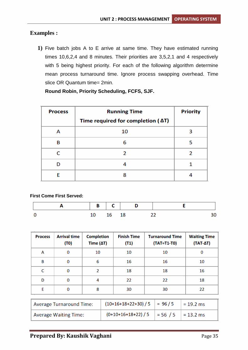
Examples :

1) Five batch jobs A to E arrive at same time. They have estimated running

times 10,6,2,4 and 8 minutes. Their priorities are 3,5,2,1 and 4 respectively

with 5 being highest priority. For each of the following algorithm determine

mean process turnaround time. Ignore process swapping overhead. Time

slice OR Quantum time= 2min.

Round Robin, Priority Scheduling, FCFS, SJF.

First Come First Served:



Shortest Job First:

Priority:



Round Robin:

2) Suppose that the following processes arrive for the execution at the times

indicated. Each process will run the listed amount of time. Assume

preemptive scheduling.

What is the turnaround time for these processes with Shortest Job First

scheduling algorithm?

3) Consider the following set of processes with length of CPU burst time

given in milliseconds.



Assume arrival order is: P1, P2, P3, P4, P5 all at time 0 and a smaller

priority number implies a higher priority. Draw the Gantt charts

illustrating the execution of these processes using preemptive priority

scheduling.

unit 2 : process management - wordpress.com · unit 2 : process management operating system...

Documents