unit 2 frequency distribution and skewness - …€¦ · unit 2 frequency distribution and skewness...
TRANSCRIPT
UNIT 2 FREQUENCY DISTRIBUTION AND
SKEWNESS

Frequency Distributionand Skewness
NOTES
Self-Instructional Material 77
UNIT 2 FREQUENCY DISTRIBUTIONAND SKEWNESS
Structure2.0 Introduction2.1 Unit Objectives2.2 Frequency Distribution
2.2.1 Constructing a Frequency Distribution2.2.2 Preparing a Frequency Distribution Table
2.3 Frequency Distribution and Measures of Central Tendency2.3.1 Descriptive Statistics2.3.2 Measures of Central Tendency2.3.3 Arithmetic Mean2.3.4 Median2.3.5 Mode
2.4 Variations2.5 Dispersion
2.5.1 Measures of Dispersion: Definition2.5.2 The Range2.5.3 Types of Measures2.5.4 Merits, Limitations and Characteristics of Measures
2.6 Skewness2.6.1 Measures of Skewness
2.7 Summary2.8 Key Terms2.9 Answers to ‘Check Your Progress’
2.10 Questions and Exercises2.11 Further Reading
2.0 INTRODUCTION
In this unit, you will learn about frequency distribution and skewness. For a properunderstanding of the quantitative data, they should be classified and convertedinto a frequency distribution. A frequency distribution is defined as the list of all thevalues obtained in the data and the corresponding frequency with which thesevalues occur in the data. The various methods of measurement of the centraltendency are mean, median and mode. You will learn the arithmetic proceduresthat can be used for analysing and interpreting quantitative data, i.e. the concept ofarithmetic mean, median and mode, but classification is only the first step in statisticalanalysis.
This unit will also introduce you to data variations. Variance or coefficient ofvariation has the same properties as standard deviation and is the square of standarddeviation, represented as σ2.
78 Self-Instructional Material
Frequency Distributionand Skewness
NOTES
The unit talks about the measures of dispersion. The measures of centraltendency are computed to see through the variability or dispersion of the individualvalues, but the dispersion is in itself a very important property of a distribution andneeds to be measured by appropriate statistics.
You will also learn that measure of dispersion can be expressed in an ‘absoluteform’, or in a ‘relative form’. It is said to be in an absolute form when it states theactual amount by which the value of an item on an average deviates from a measureof central tendency.
2.1 UNIT OBJECTIVES
After going through this unit, you will be able to:• Understand the concept of frequency distribution• Understand the significance of central tendency in frequency distribution• Calculate variance and coefficient of variation• Understand the concept of measures of dispersion and its significance in
statistical analysis• Describe the various types of measures• Describe the characteristics, merits and limitations of measures
• Understand when frequency distribution is called skewed
2.2 FREQUENCY DISTRIBUTION
Statistical data can be organized into a frequency distribution which simply lists thevalue of the variable and the frequency of its occurrence in a tabular form. Afrequency distribution can then be defined as a list of all the values obtained in thedata and the corresponding frequency with which these values occur in the data.
The frequency distribution can be either ungrouped or grouped. When thenumber of values of the variable is small, then we can construct an ungroupedfrequency distribution, which is simply listing the frequency of occurrence againstthe value of the given variable. As an example, let us assume that 20 families weresurveyed to find out the number of children in each family. The raw data obtainedfrom the survey are as follows:
0, 2, 3, 1, 1, 3, 4, 2, 0, 3, 4, 2, 2, 1, 0, 4, 1, 2, 2, 3These data can be classified into an ungrouped frequency distribution. The
number of children becomes our variable (X) for which we can list the frequencyof occurrence ( f ) in a tabular form as given in Table 2.1.

Frequency Distributionand Skewness
NOTES
Self-Instructional Material 79
Table 2.1 Data Classification
Number of Children (X) Frequency ( f )0 31 42 63 44 3
Total = 20
Table 2.1 is also known as discrete frequency distribution, where the variablehas discrete numerical values.
However, when the data set is very large, it becomes necessary to condensethe data into a suitable number of groups or classes of the variable values and thenassign the combined frequencies of these values into their respective classes. Asan example, let us assume that 100 employees in a factory were surveyed to findout their ages. The youngest person was 20 years of age and the oldest was 50years old. We can construct a grouped frequency distribution for these data sothat instead of listing frequency by every year of age, we can list frequency accordingto an age group. Also, since age is a continuous variable, the frequency distributionwould be as given in Table 2.2.
Table 2.2 Frequency Distribution
Age Group (Years) Frequency20 to less than 25 525 ” ” ” 30 1530 ” ” ” 35 2535 ” ” ” 40 3040 ” ” ” 45 1545 ” ” ” 50 10
Total = 100
In this example, all persons between 20 years (including 20 years old) and25 years (but not including 25 years old) would be grouped in the first class, andso on. The interval of 20 to less than 25 is known as class interval (CI). A singlerepresentation of a class interval would be the midpoint (or average) of that classinterval. The midpoint is also known as the class mark.
2.2.1 Constructing a Frequency Distribution
The number of groups and the size of class intervals are more or less arbitrary innature within the general guidelines established for constructing a frequencydistribution. The following guidelines for such a construction may be considered:

80 Self-Instructional Material
Frequency Distributionand Skewness
NOTES
(i) The classes should be clearly defined and each of the observations shouldbe included in only one of the class intervals. This means that the intervalsshould be chosen in such a manner that one score cannot belong to morethan one class interval, so that there is no overlapping of class intervals.
(ii) The number of classes should neither be too large nor too small. Normally,between six and fifteen classes are considered to be adequate. Fewer classintervals would mean a greater class interval width with consequent loss ofaccuracy. Too many class intervals result in greater complexity.
(iii) All intervals should be of the same width. This is preferred for easycomputations. A suitable class width can be obtained by knowing the rangeof data (which is the absolute difference between the highest value and thelowest value in the data) and the number of classes which are predetermined,so that
RangeThe width of the interval =Number of classes
In the case of ages of factory workers where the youngest worker was 20years old and the oldest was 50 years old, the range would be 50 – 20 =30. If we decide to make 10 groups, then the width of each class would be:
30/10 = 3Similarly, if we decide to make 6 classes instead of 10, then the width ofeach class interval would be:
30/6 = 5(iv) Open-ended cases—where there is no lower limit of the first group or no
upper limit of the last group—should be avoided since this creates difficultyin analysis and interpretation. (The lower and the upper values of a classinterval are known as lower and upper limits.)
(v) Intervals should be continuous throughout the distribution. For example, inthe case of factory workers, we could put them in groups of 20 to 24 years,then 25 to 29 years, and so on, but it would be highly misleading because itdoes not accurately represent the person who is between 24 and 25 yearsor between 29 and 30 years, and so on. Accordingly, it is morerepresentative to group them as 20 years to less than 25 years and25 years to less than 30 years. In this way, everybody who is 20 years anda fraction less than 25 years is included in the first category and the personwho is exactly 25 years and above but a fraction less than 30 years wouldbe included in the second category, and so on. This is especially importantfor continuous distributions.
(vi) The lower limits of class intervals should be simple multiples of the intervalwidth. This is primarily for the purpose of simplicity in construction andinterpretation. In our example of 20 years but less than 25 years, 25 years

Frequency Distributionand Skewness
NOTES
Self-Instructional Material 81
but less than 30 years, and 30 years but less than 35 years, the lower limitvalues for each class are simple multiples of the class width which is 5.
Example 2.1: The ages (in years) of a sample of 30 persons are as follows:20, 18, 25, 68, 23, 25, 16, 22, 29, 37,35, 49, 42, 65, 37, 42, 63, 65, 49, 42,53, 48, 65, 72, 69, 57, 48, 39, 58, 67.
Construct a frequency distribution for these data.Solution:
Follow the steps as given:1. Find the range of the data by subtracting the lowest age from the
highest age. The lowest value is 16 and the highest value is 72. Hence,the range is 72 – 16 = 56.
2. Assume that we shall have 6 classes, since the number of values is nottoo large. Now we divide the range of 56 by 6 to get the width of theclass interval. The width is 56/6 = 9.33. For the sake of convenience,assume the width to be 10 and start the first class boundary with 15 sothat the intervals would be 15 and upto 25, 25 and upto 35, and so on.
3. Combine all the frequencies that belong to each class interval and assignthis total frequency to the corresponding class interval as follows:
Class Interval (years) Tally Frequency ( f )
15 to less than 25 |||| 5
25 to less than 35 ||| 3
35 to less than 45 |||| || 7
45 to less than 55 |||| 5
55 to less than 65 ||| 3
65 to less than 75 |||| || 7
Total = 30
Conversion of a discrete list to a continuous list
In statistics, calculations are performed by arranging the large raw (ungrouped)data set into grouped data and are represented in tabular form called frequencydistribution table. The data to be grouped must be homogenous and comparable.The frequency distribution table gives the size and the number of class intervals.The range of each class is defined by the class boundaries.
The variables constitute a discrete list or a continuous list. A variable isconsidered as continuous when it can assume an infinite number of real values and it

82 Self-Instructional Material
Frequency Distributionand Skewness
NOTES
is considered discrete when it is the finite number of real values. Examples of acontinuous variable are distance, age, temperature and height measurements, whereasthose of a discrete variable are the scores given by the experts or the judgementteam for a competitive examination, basket ball match, cricket match, etc.
For a discrete list of data, the range can be defined as 0 – 4, 5 – 9, 10 – 14,and so on. Similarly, the range of data for a continuous list can be defined as10 – 20, 20 – 30, 30 – 40, and so on.
In a class interval, the end points define the lowest and the highest valuesthat a variable can take. In this example, if we consider the data set for age, thenthe class intervals are 0 to 4 years, 5 to 9 years, 10 to 14 years, and 14 years andabove. For a discrete variable, the end points of the first class interval are 0 and 4,but for a continuous variable it will be 0 and 4.999. In this way, the discretevariables can be converted into continuous variables and vice versa.
Conversion of an ungrouped list into a grouped listThe data collected first-hand for any statistical evaluation are considered as rawor ungrouped data as these are not meaningful and do not present a clear picture.These are then arranged in the ascending or the descending order in a tabular formcalled array. Example 2.2 will make the concept more clear.Example 2.2: The following table shows the daily wages (in Rs) of 40 workers.Convert the ungrouped data into grouped data and also prepare a discrete frequencytable with tally marks.
Ungrouped Data
90 85 50 70 55 86 60 75 80 65
75 78 86 80 60 90 55 95 65 85
55 70 60 85 80 95 90 75 60 86
60 95 85 70 65 55 86 90 80 78
Solution: After arranging this into grouped data, we get the following table:Grouped Data
95 95 95 90 90 90 90 86 86 86
86 85 85 85 85 80 80 80 80 78
78 75 75 75 70 70 70 65 65 65
60 60 60 60 60 55 55 55 55 50

Frequency Distributionand Skewness
NOTES
Self-Instructional Material 83
The discrete frequency distribution of daily wages with tally marks:
Daily Wages
Tally Marks Frequency
95 ||| 3
90 |||| 4
86 |||| 4
85 |||| 4
80 |||| 4
78 || 2
75 ||| 3
70 ||| 3
65 ||| 3
60 |||| 5
55 |||| 4
50 | 1
Class intervals of unequal width
From the data given in Example 2.2, a table showing class intervals of unequalwidth is drawn.
Daily Wages Tally Marks Frequency
50 – 55 |||| 5
55 – 60 |||| 5
60 – 65 ||| 3
65 – 70 ||| 3
70 – 75 ||| 3
75 – 78 || 2
78 – 80 |||| 4
80 – 85 |||| 4
85 – 86 |||| 4
86 – 90 |||| 4
90 – 95 ||| 3
Total 40

84 Self-Instructional Material
Frequency Distributionand Skewness
NOTES
Cumulative frequency distribution
While the frequency distribution table tells us the number of units in each classinterval, it does not tell us directly the total number of units that lie below or abovethe specified values of class intervals. This can be determined from a cumulativefrequency distribution. When the interest of the investigator focuses on the numberof items below a specified value, then this specified value is the upper limit of theclass interval. It is known as less than cumulative frequency distribution. Similarly,when the interest lies in finding the number of cases above a specified value, thenthis value is taken as the lower limit of the specified class interval and is known asmore than cumulative frequency distribution. The cumulative frequency simply meanssumming up the consecutive frequencies as follows (taking Example 2.1):
Class Interval (Years) ( f ) Cumulative Frequency (Less than)
15 and up to 25 5 5 (less than 25)
25 and up to 35 3 8 (less than 35)
35 and up to 45 7 15 (less than 45)
45 and up to 55 5 20 (less than 55)
55 and up to 65 3 23 (less than 65)
65 and up to 75 7 30 (less than 75)
Similarly, the following is the greater than cumulative frequency distribution:
Class Interval (Years) ( f ) Cumulative Frequency (Greater than)
15 and up to 25 5 30 (greater than 15)
25 and up to 35 3 25 (greater than 25)
35 and up to 45 7 22 (greater than 35)
45 and up to 55 5 15 (greater than 45)
55 and up to 65 3 10 (greater than 55)
65 and up to 75 7 7 (greater than 65)
In this greater than cumulative frequency distribution, 30 persons are olderthan 15, 25 are older than 25, and so on.
2.2.2 Preparing a Frequency Distribution Table
If a frequency table records the distribution of a discrete variable, then the real andthe apparent class limits are the same (unless the class interval is exclusive). This isdue to the fact that discrete data are always expressed in whole numbers and arealways characterized by gaps at which no measure may ever be found. Thus, if theclass intervals of discrete variable are
6–10 11–15 16–20

Frequency Distributionand Skewness
NOTES
Self-Instructional Material 85
the apparent limits 6 and 10, 11 and 15, 16 and 20 are real limits. The class 6–10includes only those items whose sizes are 6, 7, 8, 9 or 10. Any item whose size ismore than 10, i.e. 11, 12, etc., or less than 6, i.e. 5 is not included in this class, butin the next higher or the next lower class. There are, of course, no values between10 and 11 or 15 and 16. In such a case, the midpoint is the middle of the fivevalues included in a class, namely 8 is the midpoint in 6–10 class, 13 is the midpointin 11–15 class, and 18 is the midpoint in 16–20 class.
If, however, the class interval is exclusive, the apparent limits are not real andbefore finding the midpoint, the real limits should be determined. If the class intervalis given in the following manner, it is said to be an exclusive class interval:
(i) 5–10 (ii) 10–15 (iii) 15–20This means that an item having a value 15 is to be included either in class (ii) or
class (iii). If it is included in class (ii) it means value 10 is included in class (i).Hence, the real limits of class (ii) are 11–15 and the midpoint is 13. If 15 is notincluded in class (ii) but is included in class (iii) the real limits of class (ii) are then10–14 and the midpoint is 12. It, therefore, follows that whenever we have anexclusive class interval, we must decide as to which limit of the class is excludedand only then the midpoint should be ascertained.
If the frequency table records the distribution of a continuous variable, thenthe real limits are not the same as the apparent limits. This is because theoreticallysuch variables can be measured to an infinitesimal fraction of a unit, and the measuresthat are obtained are only approximations to absolute accuracy. While measuringthe weight of boys, for example, we seldom go to a unit smaller than the pound.Thus, when we say that the weight of an individual is 140 pounds, what we reallymean is that his weight is nearer 140 pounds than 139 or 141 pounds. This meansthat it is somewhere between 139.5 and 140.5 pounds.
From this, it follows that if in any frequency distribution of weights we find aclass interval identified by the interval limit (say, 140–144), we must conclude that(a) weights have been measured correct to the nearest pound and (b) hence, thereal limits of the interval extend by 0.5 pounds on either side and class interval,strictly speaking, is 139.5–144.5. The midpoint of this class is to be determinedfrom these limits. The method of finding the mid-value in this case is as follows:
Lower limit of the class + Upper limit Lower limit2− = 139 5 5
2. + = 139.5 +
2.5 = 142.0
or Upper limit Lower limit2+ = 139 5 144 5
2284
2. .+
= = 142.0
If the weight has been measured correct to the nearest tenth of a pound, wewill have class intervals like the following:
140 – 144.9145 – 149.9
86 Self-Instructional Material
Frequency Distributionand Skewness
NOTES
On the basis of what has been said earlier, the real limits are:139.95 – 144.95144.95 – 149.95
Here the midpoint will be, 139 95 144 952
. .+ = 142.45, i.e. 142.5
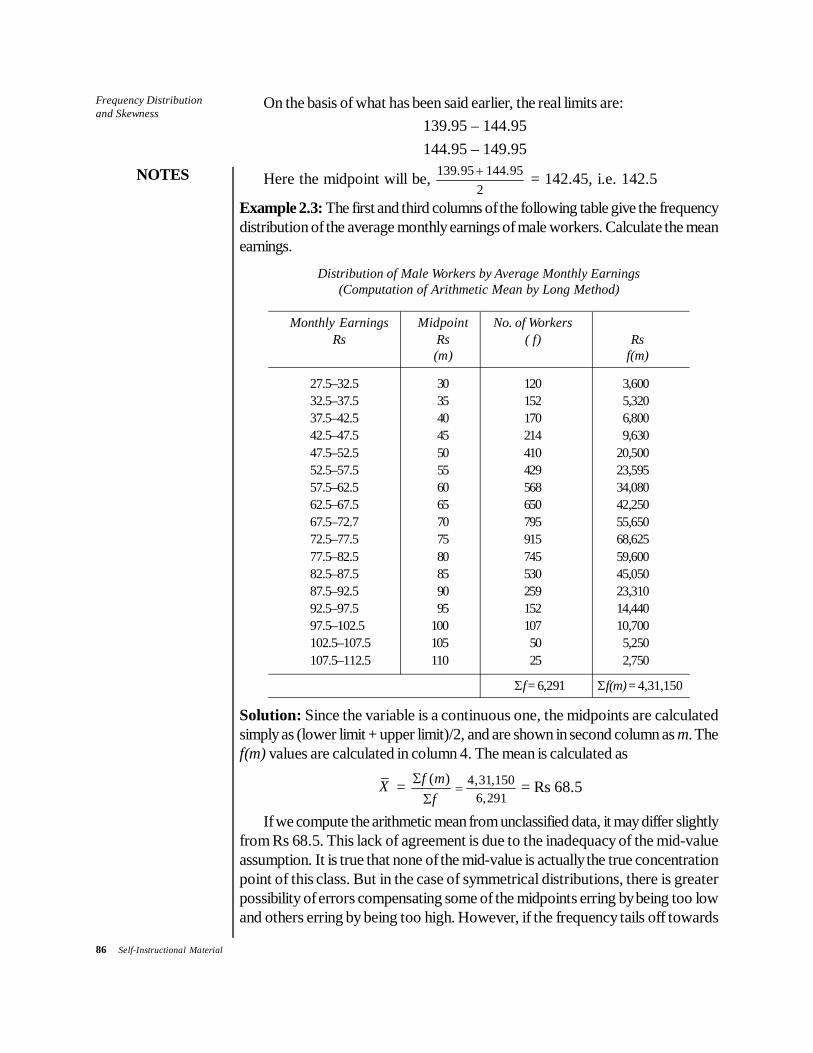
Example 2.3: The first and third columns of the following table give the frequencydistribution of the average monthly earnings of male workers. Calculate the meanearnings.
Distribution of Male Workers by Average Monthly Earnings(Computation of Arithmetic Mean by Long Method)
Monthly Earnings Midpoint No. of WorkersRs Rs ( f) Rs
(m) f(m)
27.5–32.5 30 120 3,60032.5–37.5 35 152 5,32037.5–42.5 40 170 6,80042.5–47.5 45 214 9,63047.5–52.5 50 410 20,50052.5–57.5 55 429 23,59557.5–62.5 60 568 34,08062.5–67.5 65 650 42,25067.5–72.7 70 795 55,65072.5–77.5 75 915 68,62577.5–82.5 80 745 59,60082.5–87.5 85 530 45,05087.5–92.5 90 259 23,31092.5–97.5 95 152 14,44097.5–102.5 100 107 10,700102.5–107.5 105 50 5,250107.5–112.5 110 25 2,750
Σf = 6,291 Σf(m) = 4,31,150
Solution: Since the variable is a continuous one, the midpoints are calculatedsimply as (lower limit + upper limit)/2, and are shown in second column as m. Thef(m) values are calculated in column 4. The mean is calculated as
X = ( )f mf
ΣΣ
= 4 31 1506 291, ,
, = Rs 68.5
If we compute the arithmetic mean from unclassified data, it may differ slightlyfrom Rs 68.5. This lack of agreement is due to the inadequacy of the mid-valueassumption. It is true that none of the mid-value is actually the true concentrationpoint of this class. But in the case of symmetrical distributions, there is greaterpossibility of errors compensating some of the midpoints erring by being too lowand others erring by being too high. However, if the frequency tails off towards

Frequency Distributionand Skewness
NOTES
Self-Instructional Material 87
either the high or low values, i.e. if it departs seriously from a symmetrical distribution,the arithmetic average computed will be somewhat in error because of the failureof the known errors in the midpoints assumption to compensate.
CHECK YOUR PROGRESS
1. Differentiate a continuous variable from a discrete variable.2. What is the less than cumulative frequency distribution?
2.3 FREQUENCY DISTRIBUTION AND MEASURESOF CENTRAL TENDENCY
2.3.1 Descriptive Statistics
A single number describing some feature of a frequency distribution is calleddescriptive statistics. The main thrust of a statistician presenting a mass of data isto evolve few such descriptive statistics which describe the essential nature of thefrequency distribution.
For a proper appreciation of the various descriptive statistics involved, it isnecessary to note that most of the statistical distributions have some commonfeatures. Though the size of the variables varies from item to item, most of theitems are distributed in such a manner that if you move from the lowest value to thehighest value of the variable, the number of items at each successive stage increaseswith a certain amount of regularity till you reach a maximum; and then, as youproceed further, it decreases with the similar regularity. If you plot the percentagefrequency density, i.e. the percentage of cases in an interval of unit variablewidth, you get frequency curves of the type shown in Figure 2.1. (Note that thearea under each curve should be equal to 100, the total percentage points.)
Y
X
Fig. 2.1 Frequency Curves
There are various ‘gross’ ways in which frequency curves can differ from oneanother. Even when the ‘general’ shapes of the curves are the same (the area

88 Self-Instructional Material
Frequency Distributionand Skewness
NOTES
under them already made equal by the strategy of plotting the per cent density),the details of the shape may change. Thus, the curve B has a smaller spread thanA, the curve C is more peaky and curve E is less symmetrical. Even when thecurves have almost the same shape (i.e. same spread, peakiness, symmetry, etc.)as in curves A and D, the two may differ in location along the variable axis. Thus,the items of distribution D are generally larger than those of A. So also are those ofB compared to A. Hence, a kind of an ‘average’ location of the distribution alongthe variable axis is an important descriptive statistics. These statistics are collectivelyknown as measures of location or of central tendency.
2.3.2 Measures of Central Tendency
As already mentioned, these statistics indicate the location of the frequency curvealong the X-axis and ignore all other features of the distribution. There are variouspossible measures that can be used to ‘locate’ a frequency distribution, as shownin Figure 2.2.
A, the minimum value.B, the value of maximum concentration.C, the value which divides the distribution into half, such that one half of the
items have value less than this and the other half more.D, the average value of all items.E, the 95th percentile, i.e. the value below which 95 per cent items lie.F, the maximum value.
Fig. 2.2 Frequency Distribution
If the shape of the frequency distributions were fixed, then all these measuresare equally descriptive, and fix the location of the curve. But, the practicaldistributions that we deal with always have some change in shape depending onthe samples we take, even though the general shapes are quite similar. It is, therefore,necessary that we choose those measures of location which are not very sensitiveto the specific values of items, in particular the extreme values. Thus, measures A

Frequency Distributionand Skewness
NOTES
Self-Instructional Material 89
and E are generally meaningless because they depend on the values of the lowestand the highest items, respectively. The other measures, on the contrary, are lesssusceptible to extreme values because they are somehow related to the entiredistributions. Thus, we treat B, C, D and E as the most common measures oflocation. There are some more of such measures which we will consider later.
The most important object of calculating and measuring central tendency is todetermine a ‘single figure’ which may be used to represent a whole series involvingmagnitudes of the same variable. In that sense, it is an even more compactdescription of the statistical data than the frequency distribution.
Since an ‘average’ represent the entire data, it facilitates comparison withinone group or between groups of data. Thus, the performance of the members of agroup can be compared by relating it to the average performance of the group.Likewise, the achievements of groups can be compared by a comparison of theirrespective averages.
2.3.3 Arithmetic MeanThere are several commonly used measures such as arithmetic mean, mode andmedian. These values are very useful not only in presenting the overall picture ofthe entire data but also for the purpose of making comparisons among two ormore sets of data.
While arithmetic mean is the most commonly used measure of central location,mode and median are more suitable measures under certain sets of conditions andfor certain types of data. However, each measure of central tendency should meetthe following requisites.
1. It should be easy to calculate and understand.2. It should be rigidly defined. It should have only one interpretation so
that the personal prejudice or bias of the investigator does not affect itsusefulness.
3. It should be representative of the data. If it is calculated from a sample,then the sample should be random enough to be accurately representingthe population.
4. It should have sampling stability. It should not be affected by samplingfluctuations. This means that if we pick 10 different groups of collegestudents at random and compute the average of each group, then weshould expect to get approximately the same value from each of thesegroups.
5. It should not be affected much by extreme values. If few very small orvery large items are present in the data, they will unduly influence the valueof the average by shifting it to one side or other, so that the average wouldnot be really typical of the entire series. Hence, the average chosen shouldbe such that it is not unduly affected by such extreme values.

90 Self-Instructional Material
Frequency Distributionand Skewness
NOTES
Let us consider the measure of central tendency, arithmetic mean.This is also commonly known as simply the mean. Even though average, in general,means any measure of central location. When you use the word average in youdaily routine, you always mean the arithmetic average. The term is widely used byalmost every one in daily communication. You speak of an individual being anaverage student or of average intelligence. You always talk about average familysize or average family income or grade point average (GPA) for students, and soon.For discussion purposes, let us assume a variable X which stands for some scoressuch as the ages of students. Let the ages of 5 students be 19, 20, 22, 22 and 17years. Then variable X would represent these ages as follows:
X: 19, 20, 22, 22, 17
Placing the Greek symbol Σ(Sigma) before X would indicate a command that allvalues of X are to be added together. Thus,
ΣX = 19 + 20 + 22 + 22 + 17
The mean is computed by adding all the data values and dividing it by the numberof such values. The symbol used for sample average is X so that
19 20 22 22 175
X + + + +=
In general, if there are n values in the sample, then
1 2 ... nX X XXn
+ + +=
In other words,
1 , 1, 2, ...,
n
ii
XX i n
n== =∑
(2.1)
Formula (2.1) states that add up all the values of Xi where the value of i starts at 1and ends at n with unit increments so that i = 1, 2, 3, ..., n.If instead of taking a sample, you take the entire population in your calculations ofthe mean, then the symbol for the mean of the population is μ (mu) and the size ofthe population is N, so that
1 , 1, 2, ...,
N
ii
Xi N
N=μ = =∑
(2.2)

Frequency Distributionand Skewness
NOTES
Self-Instructional Material 91
If you have the data in grouped discrete form with frequencies, then the samplemean is given by
( )f XXf
Σ=
Σ (2.3)
where Σf = Summation of all frequencies= n
Σf(X) = Summation of each value of X multiplied by itscorresponding frequency ( f )
Example 2.4: Let us take the ages of 10 students as follows:
19, 20, 22, 22, 17, 22, 20, 23, 17, 18Solution: These data can be arranged in a frequency distribution as follows:
Age (X)
Frequency (f)
f(X)
17 2 34 18 1 18 19 1 19 20 2 40 22 3 66 23 1 23
Total = 10 200
In the given case, you have Σf = 10 and Σf(X) = 200, so that
X =( )f Xf
ΣΣ
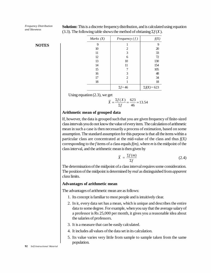
= 200/10 = 20Example 2.5: Calculate the mean of the marks of 46 students given in the followingtable.
Frequency of Marks of 46 Students
Marks Frequency(X) ( f )
9 110 211 312 613 1014 1115 716 317 218 1
Total 46
92 Self-Instructional Material
Frequency Distributionand Skewness
NOTES
Solution: This is a discrete frequency distribution, and is calculated using equation(3.3). The following table shows the method of obtianing Σf (X ).
Marks (X) Frequency ( f ) f(X)
9 1 910 2 2011 3 3312 6 7213 10 13014 11 15415 7 10516 3 4817 2 3418 1 18
Σf = 46 Σf(X) = 623
Using equation (2.3), we get
( ) 623 13.54
46f XX
fΣ
Σ= = =
Arithmetic mean of grouped dataIf, however, the data is grouped such that you are given frequency of finite-sizedclass intervals you do not know the value of every item. The calculation of arithmeticmean in such a case is then necessarily a process of estimation, based on someassumption. The standard assumption for this purpose is that all the items within aparticular class are concentrated at the mid-value of the class and thus f(X)corresponding to the f items of a class equals f(m), where m is the midpoint of theclass interval, and the arithmetic mean is then given by
X = ( )f mf
ΣΣ
(2.4)
The determination of the midpoint of a class interval requires some consideration.The position of the midpoint is determined by real as distinguished from apparentclass limits.
Advantages of arithmetic mean
The advantages of arithmetic mean are as follows:1. Its concept is familiar to most people and is intuitively clear.2. In it, every data set has a mean, which is unique and describes the entire
data to some degree. For example, when you say that the average salary ofa professor is Rs 25,000 per month, it gives you a reasonable idea aboutthe salaries of professors.
3. It is a measure that can be easily calculated.4. It includes all values of the data set in its calculation.5. Its value varies very little from sample to sample taken from the same
population.

Frequency Distributionand Skewness
NOTES
Self-Instructional Material 93
6. It is useful for performing statistical procedures such as computing andcomparing the means of several data sets.
Disadvantages of arithmetic mean
The disadvantages of arithmetic mean are as follows:1. It is affected by extreme values, and hence, is not very reliable when the
data set has extreme values, especially on one side of the ordered data.Thus, a mean of such data is not truly a representative of the data. Forexample, the average age of three persons of ages 4, 6 and 80 years givesyou an average of 30.
2. It is tedious to compute for a large data set as every point in the data set isto be used in computations.
3. It does not allow to compute the mean for a data set that has open-endedclasses either at the high or at the low end of the scale.
4. It cannot be calculated for qualitative characteristics, such as beauty orintelligence, unless these can be converted into quantitative figures, such asintelligence into IQs.
Properties of arithmetic meanThe arithmetic mean has the following interesting properties.
1. The sum of the deviations of individual values of X from the mean willalways add up to zero. This means that if you subtract all the individualvalues from their mean, then some values will be negative and some willbe positive, but if all these differences are added together, then the totalsum will be zero. In other words, the positive deviations must balance thenegative deviations, or symbolically:
1( )
n
ii
X X=
−∑ = 0, i = 1, 2, ..., n
2. The second important characteristic of the mean is that it is very sensitiveto extreme values. Since the computation of the mean is based uponinclusion of all values in the data, an extreme value in the data would shiftthe mean towards it, thereby making the mean unrepresentative of thedata.
3. The third property of the mean is that the sum of squares of the deviationsabout the mean is minimum. This means that if you take differences betweenindividual values and the mean and square these differences individually andthen add these squared differences, then the final figure will be less than thesum of the squared deviations around any other number other than the mean.Symbolically, it means that
2
1( )
n
ii
X X=
−∑ = Minimum, i = 1, 2, ..., n

94 Self-Instructional Material
Frequency Distributionand Skewness
NOTES
4. The product of the arithmetic mean and the number of values on which themean is based is equal to the sum of all given values. In other words, if youreplace each item in series by the mean, then the sum of the thesesubstitutions will equal the sum of individual items. Thus, in the figures 3,5, 7, 9, if we substitute the mean for each item, 6, 6, 6, 6 then the total is24, both in the original series and in the substitution series.This can be shown as
Since, X = X
NΣ
∴ N X = XΣFor example, you we have a series of values 3, 5, 7, 9, the mean is 6. Thesquared deviations are:
2
2
3 3 6 3 95 5 6 1 17 7 6 1 19 9 6 3 9
20
X X X X X
X
− = ′ ′− = −− = −− =− =
Σ =′
This property provides a test to check if the computed value is the correctarithmetic mean.
Example 2.6: The mean age of a group of 100 persons (grouped in intervals10–, 12–, ..., etc.) was found to be 32.02. Later, it was discovered that age 57was misread as 27. Find the corrected mean.Solution: Let the mean be denoted by X. So putting the given values in the formulaof A.M., you have,
32.02 = 100
X∑ , i.e. X∑ = 3202
Correct X∑ = 3202 – 27 + 57 = 3232
∴ Correct AM = 3232100
= 32.32
Example 2.7: The mean monthly salary paid to all employees in a company is Rs500. The monthly salaries paid to male and female employees average Rs 520and Rs 420, respectively. Determine the percentage of males and females employedby the company.Solution: Let N1 be the number of males and N2 be the number of femalesemployed by the company. Also let x1 and x2 be the monthly average salaries paidto male and female employees and x12 be the mean monthly salary paid to all theemployees.

Frequency Distributionand Skewness
NOTES
Self-Instructional Material 95
x12 = N x N xN N
1 1 2 2
1 2
++
or 500 = 520 4201 2
1 2
N NN N
++
or 20N1= 80N2
or NN
1
2= 80
2041
=
Hence, the males and females are in the ratio of 4 : 1 or 80 per cent are malesand 20 per cent are females in those employed by the company.
Short-cut methods for calculating meanYou can simplify the calculations of mean by noticing that if you subtract a constantamount A from each item X to define a new variable X' = X – A, the mean X ′ ofX' differs from X by A. This generally simplifies the calculations and you can thenadd back the constant A, termed as the assumed mean1:
X = ( )f XA X Af
′∑+ = +′∑
The following table illustrates the procedure of calculation by short-cut methodusing the data given in example 2.4. The choice of A is made in such a manner asto simplify calculation the most, and is generally in the region of the concentrationof data.
X ( f ) Deviation from f(X')Assumed Mean (13) X'
9 1 –4 –410 2 –3 –611 3 –2 –612 6 –1 –6
13 10 0 –221
14 11 +1 +1115 7 +2 +1416 3 +3 +917 2 +4 +818 1 +5 + 5
+47–22
Σf = 46 ΣfX ′ = 25
The mean,
X = ( ) 251346
f XAf
′∑+ = +∑
= 13.54
which is the same as calculated in Example 2.5.
1 Since there will not be an entry in the f(X') column corresponding to X' = 0, we write the sum –22 ofthe negative entries in the f(X') column. The sum of the positive products in the f(X') column, i.e. 47,is also written as the total N. The final sum 25 is then easily obtained.

96 Self-Instructional Material
Frequency Distributionand Skewness
NOTES
In the case of grouped frequency data, the variable X is replaced by mid-value m, and in the short-cut technique, you subtract a constant value A from eachm, so that the formula becomes:
X = Af m A
f+
−∑∑( )
In the cases where the class intervals are equal, you may further simplifycalculatation by taking the factor i from the variable m – A defining,
X' = m Ai−
Where i is the class width. It can be verified that when X' is defined, the mean ofthe distribution is given by
X = ( )f XA if
′∑+ ×∑
The following examples will illustrate the use of short-cut method.Example 2.8: The ages of twenty husbands and wives are given in the followingtable. Form a two-way frequency table showing the relationship between the agesof husbands and wives with class intervals 20–24; 25–29, etc.
Calculate the arithmetic mean of the two groups after the classification.S.No. Age of Husband Age of Wife
1 28 232 37 303 42 404 25 265 29 256 47 417 37 358 35 259 23 21
10 41 3811 27 2412 39 3413 23 2014 33 3115 36 2916 32 3517 22 2318 29 2719 38 3420 48 47

Frequency Distributionand Skewness
NOTES
Self-Instructional Material 97
Solution:Frequency Distribution of Age of Husbands and Wives
Age of Age of wifeHusband 20–24 25–29 30–34 35–39 40–44 45–49 Total
20–24 III 325–29 II III 530–34 I I 235–39 II III I 640–44 I I 245–49 I I 2
Total 5 5 4 3 2 1 20
Calculation of Arithmetic Mean of Husbands’ Age
Class Intervals Mid-values Husband x2' = m − 37
5f1x1'
m Frequency ( f1)
20–24 22 3 –3 –925–29 27 5 –2 –1030–34 32 2 –1 –2
21−
35–39 37 6 0 040–44 42 2 1 245–49 47 2 2 4
6
Σf1 = 20 Σf1x1' = –15
Arithmetic mean of husband’s ages:
x = f xN
i A1 1 1520
5 37′∑ −
+ = +× × = 33.25
Calculation of Arithmetic Mean of Wives’ Age
Wife
Class Intervals Mid-values Frequency x2' = m − 37
5f2x2'
m ( f2)
20–24 22 3 –3 –925–29 27 5 –2 –1030–34 32 2 –1 –235–39 37 6 0 040–44 42 2 1 245–49 47 1 2 2
Σf2 = 19 Σf2x2' = –17
Arithmetic mean of wives ages:
x = 2 2 5 3717
19i A
f xN
× + = × +−′∑ = 41.47

98 Self-Instructional Material
Frequency Distributionand Skewness
NOTES
The weighted arithmetic meanIn the computation of arithmetic mean, you need to give equal importance to eachobservation in the series. This equal importance may be misleading if the individualvalues constituting the series have different importance as in the following example:
The Raja Toy shop sellsToy cars at Rs 3 eachToy locomotives at Rs 5 eachToy aeroplanes at Rs 7 eachToy double-decker at Rs 9 each
What shall be the average price of the toys sold, if the shop sells 4 toys, one ofeach kind?
Mean price, i.e. x = x∑4
= Rs244
= Rs 6
In this case the importance of each observation (price quotation) is equal in asmuch as one toy of each variety has been sold. In the above computation of thearithmetic mean this fact has been taken care of by including ‘once only’ the priceof each toy.
But if the shop sells 100 toys: 50 cars, 25 locomotives, 15 aeroplanes and 10double deckers, the importance of the four price quotations to the dealer is notequal as a source of earning revenue. In fact their respective importance is equalto the number of units of each toy sold, i.e.
The importance of toy car 50The importance of locomotive 25The importance of aeroplane 15The importance of double-decker 10It may be noted that 50, 25, 15, 10 are the quantities of the various classes of
toys sold. It is for these quantities that the term ‘weights’ is used in statisticallanguage. Weight is represented by symbol ‘w’, and Σw represents the sum ofweights.
While determining the ‘average price of toy sold’, these weights are of greatimportance and are taken into account in the manner illustrated below:
x = 1 1 2 2 3 3 4 4
1 2 3 4
w x w x w x w xw w w w+ + ++ + +
= wxw
∑∑
When w1, w2, w3, w4 are the respective weights of x1, x2, x3, x4 which in turnrepresent the price of four varieties of toys, namely car, locomotive, aeroplaneand double-decker, respectively.
x = (50 3) (25 5) (15 7) (10 9)50 25 15 10
¥ + ¥ + ¥ + ¥+ + +
= (150) (125) (105) (90)100
+ + + = 470100
= Rs 4.70

Frequency Distributionand Skewness
NOTES
Self-Instructional Material 99
The following table summarizes the steps taken in the computation of theweighted arithmetic mean.
Weighted Arithmetic Mean of Toys Sold by the Raja Toy Shop
Toys Price per Toy Number Sold Price × WeightRs x w xw
Car 3 50 150Locomotive 5 25 125Aeroplane 7 15 105Double Decker 9 10 90
Σw = 100 Σxw = 470
Σw = 100; Σwx = 470
x = wxw
∑∑
= 470100
= 4.70
The weighted arithmetic mean is particularly useful where you have to computethe mean of means. If you are given two arithmetic means, one for each of twodifferent series, in respect of the same variable, and are required to find thearithmetic mean of the combined series, the weighted arithmetic mean is the onlysuitable method of its determination.
Example 2.9: The arithmetic mean of daily wages of two manufacturing concernsA Ltd. and B Ltd. is Rs 5 and Rs 7, respectively. Determine the average dailywages of both concerns if the numbers of workers employed were 2000 and4000, respectively.Solution: (i) Multiply each average (namely 5 and 7) by the number of workers inthe concern it represents.
(ii) Add up the two products obtained in (i).(iii) Divide the total obtained in (ii) by the total number of workers.
Weighted Mean of Mean Wages of A Ltd. and B Ltd.
Manufacturing Mean Wages Workers Mean Wages ×Concern x Employed Workers Employed
w wx
A Ltd. 5 2000 10,000B Ltd. 7 4000 28,000
w∑ = 6,000 wx∑ = 38,000
x = wxw
ÂÂ
= 38,0006,000
= Rs 6.33

100 Self-Instructional Material
Frequency Distributionand Skewness
NOTES
The preceding examples explain that ‘arithmetic means and percentage’ arenot original data. They are derived figures and their importance is relative to theoriginal data from which they are obtained. This relative importance must be takeninto account by weighting while averaging them (means and percentage).
2.3.4 Median
The second measure of central tendency that has a wide usage in statistical worksis the median. Median is that value of a variable which divides the series in such amanner that the number of items below it is equal to the number of items above it.In other words, half the total number of observations lie below the median, andhalf above it. The median is thus a positional average.
The median of ungrouped data is found easily if the items are first arranged inorder of magnitude. The median may then be located simply by counting, and itsvalue can be obtained by reading the value of the middle observations. If you havefive observations whose values are 8, 10, 1, 3 and 5, the values are first arrayed:1, 3, 5, 8 and 10. It is now apparent that the value of the median is 5, since twoobservations are below that value and two observations are above it. When thereis an even number of cases, there is no actual middle item and the median is takento be the average of the values of the items lying on either side of (N + 1)/2, whereN is the total number of items. Thus, if the values of six items of a series are 1, 2, 3,5, 8 and 10. The median is the value of item number (6 + 1)/2 = 3.5, which isapproximated as the average of the third and the fourth items, i.e.(3+5)/2=4.
Thus, the steps required for obtaining median are:1. Arrange the data as an array of increasing magnitude.2. Obtain the value of the (N+ l)/2th item.Even in the case of grouped data, the procedure for obtaining median is
straightforward as long as the variable is discrete or non-continuous as is clearfrom the following example.Example 2.10: Obtain the median size of shoes sold from the following data.
Number of Shoes Sold by Size in One Year
Size Number of Pairs Cumulative Total
5 30 30
5 12 40 70
6 50 120
6 12 150 270
7 300 570
7 12 600 1170
8 950 2120
8 12 820 2940
9 750 3690

Frequency Distributionand Skewness
NOTES
Self-Instructional Material 101
9 12 440 4130
10 250 4380
10 12 150 4530
11 40 4570
11 12 39 4609
Total 4609
Solution: Median is the value of ( )N + 12
th =4609 + 1
2th = 2305th item. Since the
items are already arranged in ascending order (sizewise), the size of 2305th item iseasily determined by constructing the cumulative frequency. Thus, the median sizeof shoes sold is 81, the size of 2305th item.
In the case of grouped data with continuous variable, the determinationof median is a bit more involved. Consider an example: the data relating to thedistribution of male workers by average monthly earnings are given in the followingtable. Clearly, the median of 6291 cases is the earnings of (6291 + l)/2 = 3l46thworker arranged in ascending order of earnings.
From the cumulative frequency, it is clear that this worker has his income in theclass interval 67.5–72.5. But it is impossible to determine his exact income. You,therefore, resort to approximation by assuming that the 795 workers of this classare distributed uniformly across the interval 67.5 – 72.5. The median worker is(3146–2713) = 433rd of these 795, and hence, the value corresponding to himcan be approximated as
67 5 433795
72 5 67 5. × ( . . )+ − = 67.5 + 2.73 = 70.23
Distribution of Male Workers by Average Monthly Earnings
Group No. Monthly No. of Cumulative No.Earnings (Rs) Workers of Workers
1 27.5–32.5 120 1202 32.5–37.5 152 2723 37.5–42.5 170 4424 42.5–47.5 214 6565 47.5–52.5 410 10666 52.5–57.5 429 14957 57.5–62.5 568 20638 62.5–67.5 650 27139 67.5–72.5 795 3508
10 72.5–77.5 915 442311 77.5–82.5 745 516812 82.5–87.5 530 569813 87.5–92.5 259 595714 92.5–97.5 152 610915 97.5–102.5 107 621616 102.5–107.5 50 626617 107.5–112.5 25 6291
Total 6291

102 Self-Instructional Material
Frequency Distributionand Skewness
NOTES
The value of the median can thus be put in the form of the formula:
Me = lN
C
fi+
+−
12 ×
where l is the lower limit of the median class, i is its width, f is its frequency, C thecumulative frequency up to (but not including) the median class and N is the totalnumber of cases.
Location of median by graphical analysisThe median can quite conveniently be determined by reference to the ogive whichplots the cumulative frequency against the variable. The value of the item belowwhich half the items lie can easily be read from the ogive.Example 2.11: Obtain the median of data given in the following table.
Monthly Earnings Frequency (f) Less than More than(Greater than)
27.5 __ 0 629132.5 120 120 617137.5 152 272 601942.5 170 442 584947.5 214 656 563552.5 410 1066 522557.5 429 1495 479662.5 568 2063 422867.5 650 2713 357872.5 795 3508 278377.5 915 4423 186882.5 745 5168 112387.5 530 5698 59392.5 259 5957 33497.5 152 6109 182102.5 107 6216 65107.5 50 6266 25112.5 25 6291 0
Solution: It is clear that this is grouped data. The first class is 27.5–32.5, whosefrequency is 120, and the last class is 107.5–112.5, whose frequency is 25.
The median can also be determined by plotting both ‘less than’ and ‘morethan’ cumulative frequency as shown in Figure 2.3. It is obvious that the twocurves should intersect at the median of the data.
Quarticles, deciles and percentilesYou know that the median is the value of the item which is located at the centre ofthe array. You can define other measures which are located at other specifiedpoints. For example, the Nth percentile of an array is the value of the item suchthat N per cent items lie below it. Clearly then, the Nth percentile Pn of groupeddata is given by
Pn = l
nN C
fi+
−100 ×

Frequency Distributionand Skewness
NOTES
Self-Instructional Material 103
where l is the lower limit of the class in which nN/100th item lies, i its width, f itsfrequency, C the cumulative frequency up to (but not including) this class, and N isthe total number of items.
Fig. 2.3 Location of Median
You can similarly define the Nth decile as the value of the item below which(nN/10) items of the array lie. Clearly,
Dn = P10n = lnN C
fi+
−10 ×
The other most commonly referred to measures of location are the quartiles.nth quartile is the value of the item which lies at the n(N/5)th item. Clearly Q2, thesecond quartile is the median. For grouped data,
Qn = P l
nN C
fin25
4= +−
×

104 Self-Instructional Material
Frequency Distributionand Skewness
NOTES
Example 2.12: Find the first and the third quartiles and the 90th percentile of thedata given in the table of solution of Example 2.10.Solution: The first quartile Q1 is the value of the N/4 = 6291/4 = 1572.75th item.Thus, the appropriate class is 57.5–62.5, and by the preceding equation of decile,
Q1 = 57 51572 75 1495
5685.
( . )×+
− = 58.18
The third quartile Q3 is the value of the 3N/4 = 3 × 6291 = 4718.25th item, orQ3 class interval is 77.5–82.5. Thus,
Q3 = 77 54718 25 4423
7455.
( . )×+
− = 79.5
Similarly, P90 lies in 82.5–87.5 class interval, and
P90 = 82 55661 9 5168
5305.
( . )×+
− = 87.16
or 90 per cent workers earn less than Rs 87.16.
2.3.5 Mode
The mode is that value of the variable which occurs or repeats itself the greatestnumber of times. The mode is the most ‘fashionable’ size in the sense that it is themost common and typical, and is defined by Zizek as ‘the value occurring mostfrequently in a series (or group of items) and around which the other items aredistributed most densely.’
The mode of a distribution is the value at the point around which the items tendto be most heavily concentrated. It is the most frequent or the most commonvalue, provided that a sufficiently large number of items are available to give asmooth distribution. It will correspond to the value of the maximum point (ordinate)of a frequency distribution if it is an ‘ideal’ or smooth distribution. It may be regardedas the most typical of a series of values. The modal wage, for example, is the wagereceived by more individuals than any other wage. The model ‘hat’ size is thatwhich is worn by more persons than any other single size.
It may be noted that the occurrence of one or a few extremely high or lowvalues has no effect upon the mode. If a series of data is unclassified, not havingbeen either arrayed or put into a frequency distribution, the mode cannot be readilylocated.
For example, if seven men are receiving daily wages of Rs 5, 6, 7, 7, 7, 8 and10, it is clear that the modal wage is Rs 7 per day. If you have a series, such as 2,3, 5, 6, 7, 10 and 11, it is apparent that there is no mode.
There are several methods of estimating the value of the mode. But, it is seldomthat the different methods of ascertaining the mode give us identical results.Consequently, it becomes necessary to decide as to which method would be mostsuitable for the purpose in hand. In order that a choice of the method may be

Frequency Distributionand Skewness
NOTES
Self-Instructional Material 105
made, you should understand each of the methods and the differences that existamong them.
The four important methods of estimating mode of a series are: (i) Locatingthe most frequently repeated value in the array, (ii) estimating the mode byinterpolation, (iii) locating the mode by graphic method and (iv) estimating themode from the mean and the median. Only the last three methods are discussed inthis unit.
Estimating the mode by interpolation
In the case of continuous frequency distributions, the problem of determining thevalue of the mode is not so simple as it might have appeared from the foregoingdescription. Having located the modal class of the data, the next problem in thecase of continuous series is to interpolate the value of the mode within this ‘modal’class.
The interpolation is made by the use of any one of the following formulae:
(i) Mo = l ff f
i12
0 2+
+× ; (ii) Mo = l f
f fi2
0
0 2−
+×
or (iii) Mo = l f ff f f f
i11 0
1 0 1 2+
−− + −( ) ( )
×
where l1 is the lower limit of the modal class, l2 is the upper limit of the modalclass, f0 equals the frequency of the preceding class in value, f1 equals the frequencyof the modal class in value, f2 equals the frequency of the following class (classnext to modal class) in value and i equals the interval of the modal class.Example 2.13: Determine the mode for the data given in the following table.
Wage Group Frequency (f)
14 – 18 618 – 22 1822 – 26 1926 – 30 1230 – 34 534 – 38 438 – 42 342 – 46 246 – 50 150 – 54 054 – 58 1
Solution: In the given data, 22–26 is the modal class (since it has the largestfrequency of 19), the lower limit of the modal class is 22, its upper limit is 26, thefrequency of the preceding class is 18, and of the following class is 12. The classinterval is 4. Using the various methods of determining mode, we have
106 Self-Instructional Material
Frequency Distributionand Skewness
NOTES
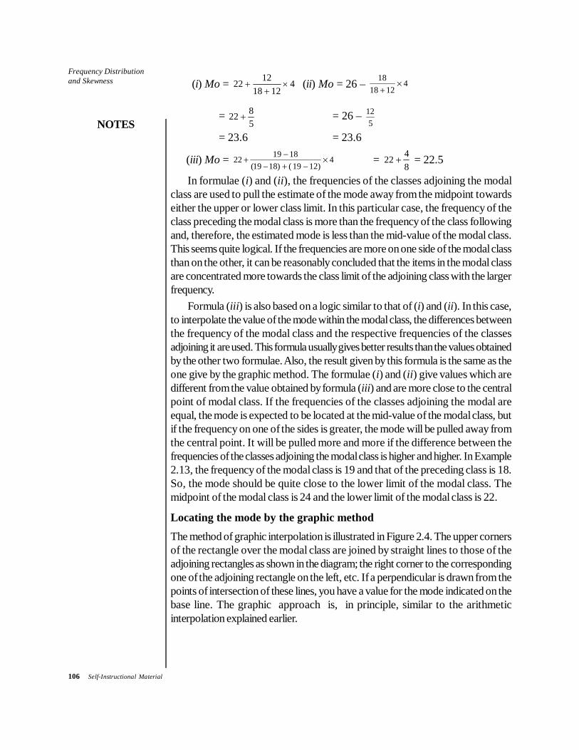
(i) Mo = 1222 418 12
+ ×+
(ii) Mo = 26 – 184
18 12¥
+
= 22 85
+ = 26 – 125
= 23.6 = 23.6
(iii) Mo = 19 1822 4
(19 18) ( 19 12)-
+ ¥- + -
= 422
8+ = 22.5
In formulae (i) and (ii), the frequencies of the classes adjoining the modalclass are used to pull the estimate of the mode away from the midpoint towardseither the upper or lower class limit. In this particular case, the frequency of theclass preceding the modal class is more than the frequency of the class followingand, therefore, the estimated mode is less than the mid-value of the modal class.This seems quite logical. If the frequencies are more on one side of the modal classthan on the other, it can be reasonably concluded that the items in the modal classare concentrated more towards the class limit of the adjoining class with the largerfrequency.
Formula (iii) is also based on a logic similar to that of (i) and (ii). In this case,to interpolate the value of the mode within the modal class, the differences betweenthe frequency of the modal class and the respective frequencies of the classesadjoining it are used. This formula usually gives better results than the values obtainedby the other two formulae. Also, the result given by this formula is the same as theone give by the graphic method. The formulae (i) and (ii) give values which aredifferent from the value obtained by formula (iii) and are more close to the centralpoint of modal class. If the frequencies of the classes adjoining the modal areequal, the mode is expected to be located at the mid-value of the modal class, butif the frequency on one of the sides is greater, the mode will be pulled away fromthe central point. It will be pulled more and more if the difference between thefrequencies of the classes adjoining the modal class is higher and higher. In Example2.13, the frequency of the modal class is 19 and that of the preceding class is 18.So, the mode should be quite close to the lower limit of the modal class. Themidpoint of the modal class is 24 and the lower limit of the modal class is 22.
Locating the mode by the graphic method
The method of graphic interpolation is illustrated in Figure 2.4. The upper cornersof the rectangle over the modal class are joined by straight lines to those of theadjoining rectangles as shown in the diagram; the right corner to the correspondingone of the adjoining rectangle on the left, etc. If a perpendicular is drawn from thepoints of intersection of these lines, you have a value for the mode indicated on thebase line. The graphic approach is, in principle, similar to the arithmeticinterpolation explained earlier.

Frequency Distributionand Skewness
NOTES
Self-Instructional Material 107
Fig. 2.4 Method of Mode Determination by Graphic Interpolation
The mode may also be determined graphically from an ogive or cumulativefrequency curve. It is found by drawing a perpendicular to the base from that pointon the curve where the curve is most nearly vertical, i.e. steepest (in other words,where it passes through the greatest distance vertically and the smallest distancehorizontally). The point where it cuts the base will give you the value of the mode.How accurately this method determines the mode is governed by (i) the shape ofthe ogive and (ii) the scale on which the curve is drawn.
Estimating the mode from the mean and the median
There usually exists a relationship among the mean, median and mode formoderately asymmetrical distributions. If the distribution is symmetrical, the mean,median and mode will have identical values, but if the distribution is skewed(moderately), the mean, median and mode will pull apart. If the distribution tailsoff towards higher values, the mean and the median will be greater than the mode.If it tails off towards lower values, the mode will be greater than either of the othertwo measures. In either case, the median will be about one-third as far away fromthe mean as the mode is. This means that
Mode = Mean – 3 (Mean – Median)= 3 Median – 2 Mean
In the case of the average monthly earnings (refer to the table of Example2.3), the mean is 68.53 and the median is 70.2. If these values are substituted inthe above formula, you get

108 Self-Instructional Material
Frequency Distributionand Skewness
NOTES
Mode = 68.5 – 3(68.5 –70.2)= 68.5 + 5.1 = 73.6
According to the formula used earlier,
Mode = l ff f
i12
0 2+
+×
= 72 5 745795 745
5. ×++
= 72.5 + 2.4 = 74.9OR
Mode = 1 0
11 0 22
f fl i
f f f−
+ ×− −
= 72 5915 795
2 915 795 7455.
××+
−− −
= 72 5 120290
5. ×+ = 75.57
The difference between the two estimates is due to the fact that the assumptionof relationship between the mean, median and mode may not always be true; it isobviously not valid in this case.Example 2.14: (a) In a moderately symmetrical distribution, the mode and meanare 32.1 and 35.4 respectively. Calculate the median.
(b) If the mode and median of moderately asymmetrical series are respectively16'' and 15.7'', what would be its most probable median?
(c) In a moderately skewed distribution, the mean and the median arerespectively 25.6 and 26.1 inches. What is the mode of the distribution?Solution: (a) You know:
Mean – Mode = 3 (Mean – Median)or 3 Median = Mode + 2 Mean
or Median = 32.1 2 35.4
3+ ¥
= 102.9
3= 34.3
(b) 2 Mean = 3 Median – Mode
or Mean = 12
3 15 7 16 0 31 12
( × . . ) .− = = 15.55
(c) Mode = 3 Median – 2 Mean= 3 × 26.1 – 2 × 25.6 = 78.3 – 51.2 = 27.1

Frequency Distributionand Skewness
NOTES
Self-Instructional Material 109
CHECK YOUR PROGRESS
3. What is descriptive statistics?4. What is the arithmetic mean.5. What are the advantages of mean?6. The following are the scores for the mid-term exam given to 13 students
in Statistics.42, 42, 68, 80, 75, 54, 62, 89, 72, 80, 80, 75, 65Calculate:(a) The mean(b) The mode(c) The median
7. The following data represent the number of cars entering a gas station onBedford Avenue for repairs between 10.00 AM and 11.00 AM in the last 8days:7, 8, 6, 8, 9, 7, 5, 6Calculate the mean for the given data.
8. The following are the monthly salaries, in rupees, of the employees in abranch bank:10, 17, 29, 95, 95, 100, 100, 175, 250 and 750Calculate the arithmetic mean.
9. The following figures represent the number of books issued at the counterof a commerce library in 11 different days.96, 180, 98, 75, 270, 20, 102, 100, 94, 75, 200Calculate the median.
2.4 VARIATIONS
The square of standard deviation, namely σ2, is termed as variance and is moreoften specified than the standard deviation. Clearly, it has the same properties asstandard deviation.As is clear, the standard deviation σ or its square, the variance, cannot be veryuseful in comparing two series where either the units are different or the meanvalues are different. Thus, a σ of 5 on an examination where the mean score is 30has an altogether different meaning than on an examination where the mean scoreis 90. Clearly, the variability in the second examination is much less. To take careof this problem, we define and use a coefficient of variation, V,
V = σx
×100 expressed as percentage.

110 Self-Instructional Material
Frequency Distributionand Skewness
NOTES
Example 2.15: The following are the scores of two batsmen A and B in a series ofinnings:
A 12 115 6 73 7 19 119 36 84 29B 47 12 76 42 4 51 37 48 13 0
Who is the better run-getter? Who is more consistent?Solution: In order to decide as to which of the two batsmen, A and B, is the betterrun-getter, you should find their batting averages. The one whose average is higherwill be considered as a better batsman.To determine the consistency in batting, you should determine the coefficient ofvariation. The less this coefficient the more consistent will be the player.
A B
Scores x x2 Scores x x2
x x
12 –38 1,444 47 14 196115 +65 4,225 12 –21 441
6 –44 1,936 76 43 1,84973 +23 529 42 9 81
7 –43 1,849 –4 – 29 84119 –31 961 51 18 324
119 +69 4,761 37 4 1636 –14 196 48 15 22584 +34 1,156 13 –20 40029 –21 441 0 –33 1,089
x∑ = 500 17,498 x∑ = 330 5,462
Batsman A: Batsman B:
x = 50010
= 50 x = 33010
= 33
σ = 17 49810, = 41.83 σ = 5 462
10, = 23.37
V = 41 83 10050
. × V = 23 3733
100. ×
= 83.66 per cent = 70.8 per cent
A is a better batsman since his average is 50 as compared to 33 of B. But B ismore consistent since the variation in his case is 70.8 as compared to 83.66 of A.Example 2.16: The following table gives the age distribution of students admittedto a college in the years 1914 and 1918. Find which of the two groups is morevariable in age.

Frequency Distributionand Skewness
NOTES
Self-Instructional Material 111
Age Number of Students
1914 1918
15 – 116 1 617 3 3418 8 2219 12 3520 14 2021 13 722 5 1923 2 324 3 –25 1 –26 – –27 1 –
Solution:
Assumed Mean—2l Assumed Mean—19Age 1914 1918
f x' fx' fx'2 f x' fx fx'2
15 0 –6 0 0 1 –4 –4 1616 1 –5 –5 25 6 –3 –18 5417 3 –4 –12 48 34 –2 –68 13618 8 –3 –24 72 22 –1 –22 22
19 12 –2 –24 48 –112
20 14 –1 –14 14
–79 35 0 0 0
21 13 0 0 0 20 1 20 2022 5 1 5 5 7 2 14 28
23 2 2 4 8 19 3 57 17124 3 3 9 27 3 4 12 48
25 1 4 4 16 147 +103 495
26 0 5 0 0 –927 1 6 6 36
63 +28 299
–51
1914 Group:
σ = fxN
fxN
′∑ −′∑L
NMOQP
2 2( )
= 29963
5163
2− −FHGIKJ

112 Self-Instructional Material
Frequency Distributionand Skewness
NOTES
= 4 476 0 655. .− = 4 091.
= 2.02
x = 21 5163
+ −FHGIKJ = 21 – 8 = 20.2
V = 2 0220 2
100..
×
= 20220 2.
= 10
1918 Group:
σ = 495147
9147
2− −FHGIKJ = 3.3673 0.0037−
= 3.3636 = 1.834
x = 19 9147
+ −FHGIKJ
= 19 – 0.06 = 18.94
V = 1 83418 94
100..
×
= 9.68The coefficient of variation of the 1914 group is 10 and that of the 1918 group9.68. This means that the 1914 group is more variable, but only barely so.Example 2.17: You are supplied the following data about the height of boys andgirls studying in a college.
Boys GirlsNumber 72 38Average height (inches) 68 61Variance of distribution 9 4You are required to find out:(a) In which sex, boys or girls, there is greater variability in individual heights.(b) Common average height of boys and girls.(c) Standard deviation of the height of boys and girls taken together.(d) Combined variability (CV).

Frequency Distributionand Skewness
NOTES
Self-Instructional Material 113
Solution:
(a) CV of boys’ height = σ1
1100 9
68100
x× ×= = 4.41%
CV of girls’ height = σ2
2100 4
61100
x× ×= = 3.28%
Thus, there is a greater variability in the height of boys than that of the girls.(b) The combined height of boys and girls is given as
x12 = N x N xN N
1 1 2 2
1 2
++
= 72 68 38 6172 38
× ×++
= 7214110
= 65.58 inches approx.
(c) The combined standard deviation may be calculated by applying thefollowing formula:
σ122 = N N
N NN x x N x x
N N1 1
22 2
2
1 2
1 12
2 22
1 2
σ σ+
++
− + −+
( ) ( )
= 72 9 38 472 38
72 65 58 68 38 65 58 6172 38
2 2× × ( . ) ( . )++
+− + −
+
= 2018 794110
. = 18.35
σ12 = 4.28 inches
(d) Combined variability = σx
× ..
×100 4 2865 58
100= = 6.53
Example 2.18: In a co-educational college, boys and girls formed separate groupson the foundation day when everyone had to put in physical labour. Computestandard deviation for boys and girls separately and for the combined group. Didthe separation by sex make each workgroup more homogeneous?
Minutes of Labour Given by No. of Girls No. of BoysEach Individual
60 20 12055 60 10050 100 20045 450 35540 450 35035 300 50030 250 35025 100 20

114 Self-Instructional Material
Frequency Distributionand Skewness
NOTES
Solution:
Minutes X' No. of f1X' f1X'2 No. of f2X' f2X2'2
of Labour45
5X −
= Girls Boys
Given byf1 f2
EachIndivi-
dual (X)60 +3 20 60 180 120 360 108055 +2 60 120 240 100 200 40050 +1 100 100 100 200 200 20045 0 450 0 0 355 0 040 –1 450 –450 450 350 –350 35035 –2 300 –600 1200 500 –1000 200030 –3 250 –750 2250 350 –1050 315025 –4 100 –400 1600 20 –80 320
Total 1730 –1920 6020 1995 –1720 7500
Girls: 1X = 45 – 19201730
× 5 = 45 – 5.55 = 39.45
σ1 = 60201730
19201730
5 3 4798 1 2317 52
− −FHG
IKJ = −× . . × = 1.5 × 5 = 7.5
V1 = 7 539 45
100..
× = 19.0%
Boys:
2X = 45 – 17201995
× 5 = 45 – 4.31 = 40.69
σ2 = 2750 1720
1995 1995−⎛ ⎞− ⎜ ⎟⎝ ⎠ × 5 = (3.7594 0.7434)− × 5
= 1.7366 × 5 = 8.68
V2 = 8 6840 69
100..
×
= 21.34%
Combined mean: 12X = 1730 39 45 1995 40 691730 1995
× . × .++
= 149424 783725
. = 40.111
d1 = 0.66 and d2 = –0.58
σ122 = 1730 7 5 1995 8 68 1730 0 66 1995 0 58
1730 1995
2 2 2 2( . ) ( . ) ( . ) ( . )+ + + −+
= 66.86σ12 = 8.18
CV = 8 1840 11
100..
× = 20.38%

Frequency Distributionand Skewness
NOTES
Self-Instructional Material 115
Therefore, there does not seem to be any evidence that each workgroup wasmore homogeneous than the total population.Example 2.19: The values of the arithmetic mean and the standard deviation ofthe following frequency distribution of a continuous variable derived from short-cut method are 135.3 lbs and 9.6 lbs respectively.
X –4 –3 –2 –1 0 1 2 3 TotalFrequency 2 5 8 18 22 13 8 4 80Determine the actual class interval.Solution: Calculation of standard deviation:
X –4 –3 –2 –1 0 1 2 3 Total
Frequency (f) 2 5 8 18 22 13 8 4 80
f(X) –8 –15 –16 –18 0 13 16 12 –16
f(X2) 32 45 32 18 0 13 32 36 208
Standard Deviation = 2( ) ( )f X f Xi
n n∑ ∑⎛ ⎞× − ⎜ ⎟⎝ ⎠
∴ Putting the known values, we have
9.6 = i × 20880
1680
2− −FHGIKJ = 2.6 0.04i × −
or 9.6 = i i× . × .2 56 1 6=
∴ i = 9 61 6..
= 6
Arithmetic mean = ( )f XA in
Σ+ ×
∴ Putting the known values, we have
135.3 = A + −1680
6× = A – 1.2
or A = 135.3 + 1.2 = 136.5A, or assumed, mean is the midpoint corresponding to the class having X value 0.As the class interval is of 6 and the variable under studying is a continuous one, theclass for which X = 0 will be 136.5 –3 to 136.5 + 3, i.e. 133.5–139.5. The classnext lower than this is 133.5–6 or 133.5, i.e. 127.5 to 133.5.
Similarly, other classes can be calculated. So all the class intervals are:109.5–115.5 115.5–121.5 121.5–127.5 127.5–133.5133.5–139.5 139.5–145.5 145.5–151.5 151.5–157.5
Determining overall performanceIf for a number of candidates each writes papers in several subjects, then the totalmarks obtained by candidates will not be a correct basis for determining their merit.

116 Self-Instructional Material
Frequency Distributionand Skewness
NOTES
This is also because the marks in different subjects are likely to have differentamounts of spread and means. The extent of the spread of marks in a paperintroduces ‘weights’ which will be to the advantage of those getting high marks insubjects where the spread is great, and to the disadvantage of those gaining highmarks in subjects where range is small.
A method to for the errors so introduced consists of converting the marks into
‘standard scores’ defined as X X−σ
. This measures deviation of marks of a student
from the mean of that subject in the units of standard deviation and are termed asz-scores as well. This corrects both for variations of X and σ in different subjects.
The z-scores of a student in different subjects are then added to give a truemeasure of relative performance.Example 2.20: Consider the following data:
Candidate Marks in
Economics Commerce TotalA 84 75 159B 74 85 159
Average for Economics is 60 with standard deviation 13Average for Commerce is 50 with standard deviation 11Based on these information, determine whose performance is better A’s or
B’s.Solution:
z-Scores A: Economics84
Commerce75
−=
−=
UV|
W|
6013
1 85
5011
2 274 12
.
..
B: Economics74
Commerce85
−=
−=
UV|
W|
6013
1 08
5011
3 284 26
.
..
Since B’s z-score is higher therefore his performance is better.
2.5 DISPERSION
2.5.1 Measures of Dispersion: Definition
A measure of dispersion, or simply dispersion may be defined as statistics signifyingthe extent of the scatteredness of items around a measure of central tendency.

Frequency Distributionand Skewness
NOTES
Self-Instructional Material 117
A measure of dispersion may be expressed in an ‘absolute form’, or in a‘relative form’. It is said to be in an absolute form when it states the actual amountby which the value of an item on an average deviates from a measure of centraltendency. Absolute measures are expressed in concrete units, i.e. units in terms ofwhich the data have been expressed, e.g. rupees, centimetres, kilograms, etc.,and are used to describe frequency distribution.
A relative measure of dispersion is a quotient obtained by dividing theabsolute measures by a quantity in respect to which absolute deviation has beencomputed. It is as such a pure number and is usually expressed in a percentageform. Relative measures are used for making comparisons between two or moredistributions.
A measure of dispersion should possess the following characteristics whichare considered essential for a measure of central tendency.
(a) It should be based on all observations.(b) It should be readily comprehensible.(c) It should be fairly and easily calculated.(d) It should be affected as little as possible by fluctuations of sampling.(e) It should be amenable to algebraic treatment.
The following are the common measures of dispersion:(i)The range, (ii) The semi-interquartile range or the quartile deviation, (iii)
The mean deviation and (iv) The standard deviation. Of these, the standard deviationis the best measure. All these measures are discussed in this unit.
2.5.2 The Range
The crudest measure of dispersion is the range of the distribution. The range ofany series is the difference between the highest and the lowest values in the series.If the marks received in an examination taken by 248 students are arranged inascending order, then the range will be equal to the difference between the highestand the lowest marks.
In a frequency distribution, the range is taken to be the difference betweenthe lower limit of the class at the lower extreme of the distribution and the upperlimit of the class at the upper extreme.

118 Self-Instructional Material
Frequency Distributionand Skewness
NOTES
Table 2.3 Weekly Earnings of Labourers in Four Workshops of the Same Type
Weekly earningsNo. of Workers
Rs Workshop A Workshop B Workshop C Workshop D
15–16 ... ... 2 ...17–18 ... 2 4 ...19–20 ... 4 4 421–22 10 10 10 1423–24 22 14 16 1625–26 20 18 14 1627–28 14 16 12 1229–30 14 10 6 1231–32 ... 6 6 433–34 ... ... 2 235–36 ... ... ... ...37–38 ... ... 4 ...
Total 80 80 80 80
Mean 25.5 25.5 25.5 25.5
Consider the data on weekly earning of worker on four workshops given in Table2.3. We note the following:
Workshop RangeA 9B 15C 23D 15
From these figures, it is clear that the greater the range, the greater is thevariation of the values in the group.
The range is a measure of absolute dispersion and as such cannot be usefullyemployed for comparing the variability of two distributions expressed in differentunits. The amount of dispersion measured, say, in pounds, is not comparable withdispersion measured in inches. So the need of measuring relative dispersion arises.
An absolute measure can be converted into a relative measure if we divideit by some other value regarded as standard for the purpose. You may use themean of the distribution or any other positional average as the standard.
From Table 2.3, the relative dispersion would be:
Workshop A = 925 5.
Workshop C = 2325 5.
Workshop B = 1525 5.
Workshop D = 1525 5.
An alternate method of converting an absolute variation into a relative one wouldbe to use the total of the extremes as the standard. This will be equal to dividingthe difference of the extreme items by the total of the extreme items. Thus,
Frequency Distributionand Skewness
NOTES
Self-Instructional Material 119
Relative dispersion = Difference of extreme items, i.e., Range
Sum of extreme items
The relative dispersion of the series is called the coefficient or ratio of dispersion.In our example of weekly earnings of workers considered earlier, the coefficientswould be:
Workshop A = 921 30
951+
= Workshop B = 1517 32
1549+
=
Workshop C = 2315 38
2353+
= Workshop D = 1519 34
1553+
=
Merits and limitations of range
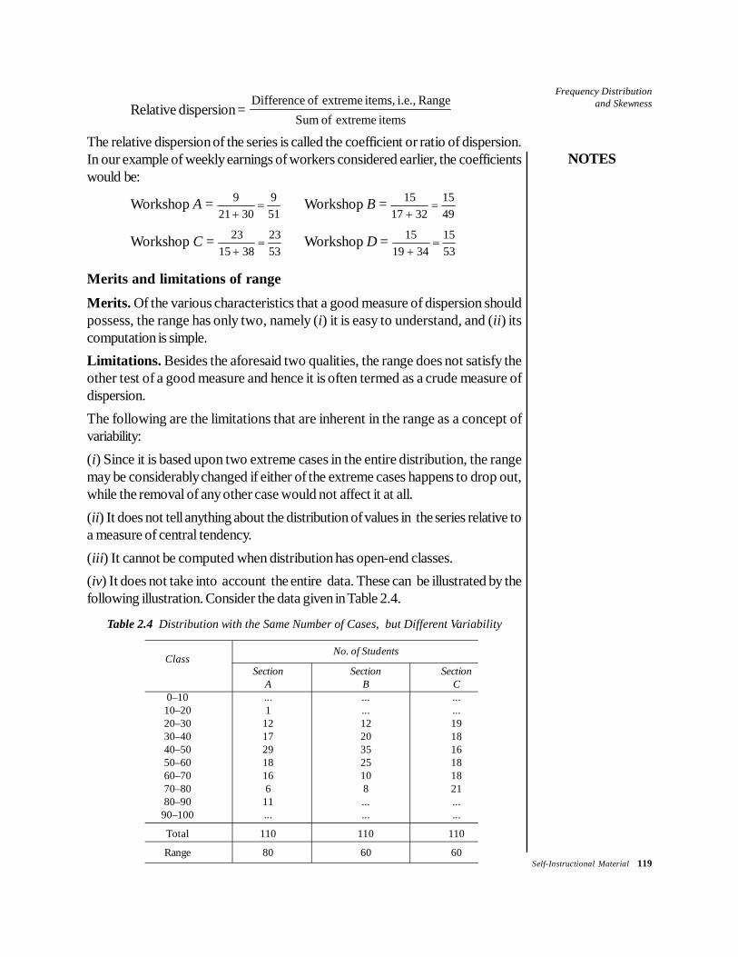
Merits. Of the various characteristics that a good measure of dispersion shouldpossess, the range has only two, namely (i) it is easy to understand, and (ii) itscomputation is simple.Limitations. Besides the aforesaid two qualities, the range does not satisfy theother test of a good measure and hence it is often termed as a crude measure ofdispersion.The following are the limitations that are inherent in the range as a concept ofvariability:(i) Since it is based upon two extreme cases in the entire distribution, the rangemay be considerably changed if either of the extreme cases happens to drop out,while the removal of any other case would not affect it at all.(ii) It does not tell anything about the distribution of values in the series relative toa measure of central tendency.(iii) It cannot be computed when distribution has open-end classes.(iv) It does not take into account the entire data. These can be illustrated by thefollowing illustration. Consider the data given in Table 2.4.
Table 2.4 Distribution with the Same Number of Cases, but Different Variability
No. of StudentsClass
Section Section SectionA B C
0–10 ... ... ...10–20 1 ... ...20–30 12 12 1930–40 17 20 1840–50 29 35 1650–60 18 25 1860–70 16 10 1870–80 6 8 2180–90 11 ... ...
90–100 ... ... ...
Total 110 110 110
Range 80 60 60

120 Self-Instructional Material
Frequency Distributionand Skewness
NOTES
The table is designed to illustrate three distributions with the same number of casesbut different variability. The removal of two extreme students from section A wouldmake its range equal to that of B or C.
The greater range of A is not a description of the entire group of 110 students,but of the two most extreme students only. Further, though sections B and C havethe same range, the students in section B cluster more closely around the centraltendency of the group than they do in section C. Thus, the range fails to reveal thegreater homogeneity of B or the greater dispersion of C. Due to this defect, it isseldom used as a measure of dispersion.
Specific uses of rangeIn spite of the numerous limitations of the range as a measure of dispersion, thereare the following circumstances when it is the most appropriate one:
• In situations where the extremes involve some hazard for which preparationshould be made, it may be more important to know the most extreme casesto be encountered than to know anything else about the distribution. Forexample, an explorer, would like to know the lowest and the highesttemperatures on record in the region he is about to enter; or an engineerwould like to know the maximum rainfall during 24 hours for the constructionof a storem water drain.
• In the study of prices of securities, range has a special field of activity. Thusto highlight fluctuations in the prices of shares or bullion it is a commonpractice to indicate the range over which the prices have moved during acertain period of time. This information, besides being of use to the operators,gives an indication of the stability of the bullion market, or that of theinvestment climate.
• In statistical quality control the range is used as a measure of variation. Forexample, you determine the range over which variations in quality are dueto random causes, which is made the basis for the fixation of control limits.
2.5.3 Types of Measures1. Quartile deviation (QD)Another measure of dispersion, much better than the range, is the semi-interquartilerange, usually termed as ‘quartile deviation’. As you know, quartiles are the pointswhich divide the array in four equal parts. More precisely, Q1 gives the value of theitem 1/4th the way up the distribution and Q3 the value of the item 3/4th the way upthe distribution. Between Q1 and Q3 are included half the total number of items.The difference between Q1 and Q3 includes only the central items but excludes theextremes. Since under most circumstances, the central half of the series tends tobe fairly typical of all the items, the interquartile range (Q3– Q1) affords a convenientand often a good indicator of the absolute variability. The larger the interquartilerange, the larger the variability.

Frequency Distributionand Skewness
NOTES
Self-Instructional Material 121
Usually, one-half of the difference between Q3 and Q1 is used and to it is given thename of quartile deviation or semi-interquartile range. The interquartile range isdivided by two for the reason that half of the interquartile range will, in a normaldistribution, be equal to the difference between the median and any quartile. Thismeans that 50 per cent items of a normal distribution will lie within the intervaldefined by the median plus and minus the semi-interquartile range.
Symbolically,
QD = Q Q3 12−
Let us find quartile deviations for the weekly earnings of labour in the four workshopwhose data is given in Table 2.3. The computations are given in Table 2.5.As shown in the table, QD of workshop A is Rs 2.12 and median value is 25.3.This means that if the distribution is symmetrical, the number of workers whosewages vary between (25.3–2.1) = Rs 23.2 and (25.3 + 2.1) = Rs 27.4, shall bejust half of the total cases. The other half of the workers will be more than Rs 2.1removed from the median wage. As this distribution is not symmetrical, the distancebetween Q1 and the median Q2 is not the same as between Q3 and the median.Hence, the interval defined by median plus and minus semi inter-quartile rangewill not be exactly the same as given by the value of the two quartiles. Under suchconditions, the range between Rs 23.2 and Rs 27.4 will not include precisely 50per cent of the workers.If QD is to be used for comparing the variability of any two series, it is necessaryto convert the absolute measure to a coefficient of quartile deviation. To do thisthe absolute measure is divided by the average size of the two quartile.
Symbolically,
Coefficient of Quartile Deviation = Q QQ Q
3 1
3 1
−+
Applying this to your illustration of four workshops, the coefficients of QD wouldbe as given in Table 2.5.
Table 2.5 Calculation of Quartile Deviation
Workshop Workshop Workshop WorkshopA B C D
Location of Q2 2N 80 40
2=
80 402
=80 402
=80 402
=
Q224.5 + 40
22−
×30 2 40 3024.5 2
18−
+ × 24.5 + 4016−
×30 2 24.5 + 40
16−
×30 2
= 24.5 + 0.9 = 24.5 + 1.1 = 24.5 + 0.75 = 24.5 + 0.75= 25.4 = 25.61 = 25.25 = 25.25

122 Self-Instructional Material
Frequency Distributionand Skewness
NOTES
Location of Q1 4N 80 20
4=
80 204
=80 204
=80 204
=
Q120 1022.5 2
22−
+ ×20 1622.5 2
14−
+ ×20 1020.5 2
10−
+ ×20 1822.5 2
16−
+ ×
= 22.5 + 0.91 = 22.5 + 0.57 = 20.5 + 2 = 22.5 + 0.25= 23.41 = 23.07 = 22.5 = 22.75
Location of Q334N 803 60
4× = 6 0 6 0 6 0
Q360 5226.5 2
14−
+ ×60 4826.5 2
16−
+ ×60 5026.5 2
12−
+ ×60 5026.5 2
12−
+ ×
= 26.5 + 1.14 = 26.5 + 1.5 = 26.5 + 1.67 = 26.5 + 1.67= 27.64 = 28.0 = 28.17 = 28.17
Quartile 3 12
Q Q− 27.64 23.412− 28 23.07
2− 28.17 22.5
2− 28 17 22 75
2. .−
Deviation = 4.23
2 = Rs 2.12 = 4.93
2 = Rs 2.46 = 5.67
2 = Rs 2.83 = 5.42
2 = Rs 2.71
Coefficient of Quartile
Deviation Q QQ Q
3 1
3 1
−+
= 27 64 23 4127 64 23 41
. .
. .−+
28 23 0728 23 07
−+
.
.28 17 22 528 17 22 5
. .
. .−+
28 17 22 7528 17 22 75
. .
. .−+
= 0.083 = 0.097 = 0.112 = 0.106
Characteristics of QD
The characteristics of quartile deviation are as follows:(i) The size of QD gives an indication about the uniformity or otherwise of the sizeof the items of a distribution. If QD is small, it denotes large uniformity. Thus, acoefficient of QD may be used for comparing uniformity or variation in differentdistributions.(ii) QD is not a measure of dispersion in the sense that it does not show thescatter around an average, but it shows only a distance on scale. Consequently,quartile deviation is regarded as a measure of partition.(iii) QD can be computed when the distribution has open-end classes.
Limitations of QD
Except for the fact that its computation is simple and it is easy to understand, a QDdoes not satisfy any other test of a good measure of variation.
2. Mean deviation (MD)A weakness of the measures of dispersion, based upon the range or a portionthereof, is that the precise size of most of the variants has no effect on the result.As an illustration, QD will be the same whether the variates between Q1 and Q3are concentrated just above Q1 or they are spread uniformly from Q1 to Q3. Thisis an important defect from the viewpoint of measuring the divergence of thedistribution from its typical value. The mean deviation is employed to overcomethis problem.

Frequency Distributionand Skewness
NOTES
Self-Instructional Material 123
Mean deviation, also called average deviation, of a frequency distribution is themean of the absolute values of the deviation from some measure of central tendency.In other words, mean deviation is the arithmetic average of the variations (deviations)of the individual items of the series from a measure of their central tendency.You can measure the deviations from any measure of central tendency, but themost commonly employed ones are the median and the mean. The median ispreferred because it has the important property that the average deviation from itis the least.Calculation of the mean deviation then involves the following steps:
(a) Calculate the median or the mean, Md or Me ( X ).
(b) Record the deviations | d | = | x – Me | of each of the items, ignoring thesign.
(c) Find the average value of deviations.
Mean deviation = | |dN
Σ
Example 2.21: Calculate the mean deviation from the following data giving marksobtained by 11 students in a class test.
14, 15, 23, 20, 10, 30, 19, 18, 16, 25, 12
Solution: Median = Size of 11 + 12
th item
= Size of 6th item = 18
Serial No. Marks | x – Median || d |
1 10 82 12 63 14 44 15 35 16 26 18 07 19 18 20 29 23 5
10 25 711 30 12
| |d∑ = 50
Mean deviation from median = | |dN
∑
= 5011
= 4.5 marks
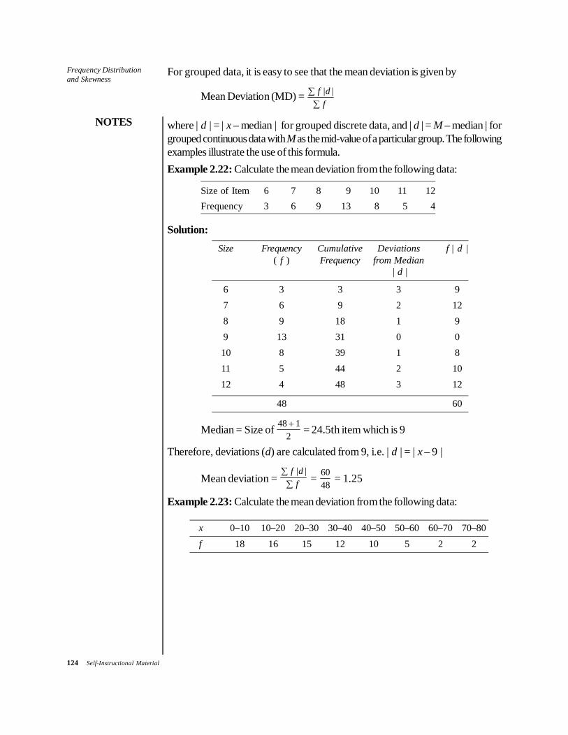
124 Self-Instructional Material
Frequency Distributionand Skewness
NOTES
For grouped data, it is easy to see that the mean deviation is given by
Mean Deviation (MD) = f df| |∑
∑
where | d | = | x – median | for grouped discrete data, and | d | = M – median | forgrouped continuous data with M as the mid-value of a particular group. The followingexamples illustrate the use of this formula.Example 2.22: Calculate the mean deviation from the following data:
Size of Item 6 7 8 9 10 11 12Frequency 3 6 9 13 8 5 4
Solution:Size Frequency Cumulative Deviations f | d |
( f ) Frequency from Median | d |
6 3 3 3 97 6 9 2 128 9 18 1 99 13 31 0 010 8 39 1 811 5 44 2 1012 4 48 3 12
48 60
Median = Size of 48 12+ = 24.5th item which is 9
Therefore, deviations (d) are calculated from 9, i.e. | d | = | x – 9 |
Mean deviation = f d
f| |∑
∑ = 6048
= 1.25
Example 2.23: Calculate the mean deviation from the following data:
x 0–10 10–20 20–30 30–40 40–50 50–60 60–70 70–80f 18 16 15 12 10 5 2 2

Frequency Distributionand Skewness
NOTES
Self-Instructional Material 125
Solution: This is a frequency distribution with continuous variable. Thus, deviationsare calculated from mid-values.
x Mid-value f Less than Deviation f | d |cf from Median
| d |
0–10 5 18 18 19 34210–20 15 16 34 9 14420–30 25 15 49 1 1530–40 35 12 61 11 13240–50 45 10 71 21 21050–60 55 5 76 31 15560–70 65 2 78 41 8270–80 75 2 80 51 102
80 1182
Median= Size of 802
th item
= 20 615
10+ × = 24
and then
Mean deviation = f d
f| |∑
∑
= 118280
= 14.775
Merits and demerits of the mean deviation
Merits: The merits of the mean deviation are as follows:
(i) It is easy to understand.(ii) As compared to standard deviation (discussed later), its computation is
simple.(iii) As compared to standard deviation, it is less affected by extreme values.(iv) Since it is based on all values in the distribution, it is better than range or
quartile deviation.
Demerits: The demerits of the mean deviation are as follows:
(i) It lacks those algebraic properties which would facilitate its computationand establish its relation to other measures.
(ii) Due to the above factor, it is not suitable for further mathematical processing.
Coefficient of mean deviationThe coefficient or relative dispersion is found by dividing the mean deviations (ifdeviations are recorded either from the mean or from the median) by mean or bymedian. Thus,

126 Self-Instructional Material
Frequency Distributionand Skewness
NOTES
Coefficient of mean deviation = Mean DeviationMean
(when deviations are recorded from the mean)
= Mean Deviation
Median(when deviations are recorded from the median)
Applying the preceding formula to Example 2.23,
Coefficient of mean deviation = 14.77524
= 0.616
3. Standard deviationBy far the most universally used and the most useful measure of dispersion is thestandard deviation (SD) or root mean square deviation about the mean. You haveseen that all the methods of measuring dispersion so far discussed are not universallyadopted for want of adequacy and accuracy. The range is not satisfactory as itsmagnitude is determined by most extreme cases in the entire group. Further, therange is notable because it is dependent on the item whose size is largely matter ofchance. The mean deviation method is also an unsatisfactory measure of scatter,as it ignores the algebraic signs of deviation. We desire a measure of scatter whichis free from these shortcomings. To some extent, SD is one such measure.
The calculation of SD differs in the following respects from that of meandeviation. First, in calculating SD, the deviations are squared. This is done so as toget rid of negative signs without committing algebraic violence. Further, the squaringof deviations provides added weight to the extreme items, a desirable feature forcertain types of series.
Secondly, the deviations are always recorded from the arithmetic mean,because although the sum of deviations is the minimum from the median, the sumof squares of deviations is minimum when deviations are measured from thearithmetic average. The deviation from x is represented by d.
Thus, SD, σ (sigma) is defined as the square root of the mean of the squaresof the deviations of individual items from their arithmetic mean.
σ = ( )x xN−∑ 2
(2.5)
For grouped data (discrete variables),
σ = f x xf
( )−∑∑
2(2.6)
and, for grouped data (continuous variables),
σ = f M xf
( )−∑∑
(2.7)

Frequency Distributionand Skewness
NOTES
Self-Instructional Material 127
where M is the mid-value of the group.The use of these equations is illustrated by the following examples.
Example 2.24: Compute the standard deviation for the following data:11, 12, 13, 14, 15, 16, 17, 18, 19, 20, 21
Solution: Here equation (2.5) is appropriate. We first calculate the mean asx = x N/∑ = 176/11 = 16, and then calculate the deviation as follows:
x (x – x ) (x – x )2
11 –5 2512 –4 1613 –3 914 –2 415 –1 116 0 017 +1 118 +2 419 +3 920 +4 1621 +5 25
176 11
Thus by formula (2.5)
σ = 11011
10= = 3.16
Example 2.25: Find the standard deviation of the data in the following distributions:
x 12 13 14 15 16 17 18 20
f 4 11 32 21 15 8 6 4
Solution: For this discrete variable grouped data, you use equation (2.6). Sincefor calculation of x , you need fx∑ and then for σ you need f x x( )−∑ 2 , thecalculations are conveniently made in the following format.
x f fx d = x – x d2 fd2
12 4 48 –3 9 3613 11 143 –2 4 4414 32 448 –1 1 3215 21 315 0 0 016 15 240 1 1 1517 8 136 2 4 3218 5 90 3 9 4520 4 80 5 25 100
100 1500 304

128 Self-Instructional Material
Frequency Distributionand Skewness
NOTES
Here x = /fx f∑ ∑ = 1500/100 = 15
and σ = fdf
2∑∑
= 304100 = 3 04. = 1.74
Example 2.26: Calculate the standard deviation of the following data:
Class 1–3 3–5 5–7 7–19 9–11 11–13 13–15 Frequency 1 9 25 35 17 10 3
Solution: This is an example of continuous frequency series and equation (2.7)seems appropriate.
Class Mid- Frequency Deviation Squared Squaredpoint of Mid- Deviation Deviation
point (x) Times(x) ( f ) f (x) from d2 Frequency
Mean (d) fd2
1–3 2 1 2 –6 36 363–5 4 9 36 –4 16 1445–7 6 25 150 –2 4 1007–9 8 35 280 0 0 0
9–11 10 17 170 2 4 6811–13 12 10 120 4 16 16013–15 14 3 42 6 36 108
100 800 616
First the mean is calculated as:
x = /fx fΣ Σ = 800/100 = 8.0
Then the deviations are obtained from 8.0.
Thus, σ = f M xf
∑ −∑
( )2
σ = fdf
2 616100
∑∑
= = 2.48
Calculation of SD by short-cut methodThe three examples worked out above have one common simplifying feature,namely x in each case turned out to be an integer, thereby, simplifying calculations.In most cases, it is very unlikely that it will turn out to be so. In such cases, thecalculation of d and d2 becomes quite time-consuming. Thus, short-cut methodshave been developed. These are on the same lines as those for calculation of meanitself.
In the short-cut method, you have to calculate deviations x' from an assumedmean A. Then, for ungrouped data,

Frequency Distributionand Skewness
NOTES
Self-Instructional Material 129
σ = ′∑ −′∑F
HGIKJ
xN
xN
2 2(2.8)
and for grouped data,
σ = 22fx fx
f f⎛ ⎞Σ Σ′ ′
− ⎜ ⎟Σ ⎝ Σ ⎠ (2.9)
These formulae are valid for both discrete and continuous variables. In caseof continuous variables, x in the equation x' = x – A stands for the mid-value of theclass in question.
Note that the second term in each of the formulae is a correction termbecause of the difference in the values of A and x . When A is taken as x itself, thiscorrection is automatically reduced to zero. The following examples explain theuse of these formulae.Example 2.27: Compute the standard deviation by the short-cut method for thefollowing data:
11, 12, 13, 14, 15, 16, 17, 18, 19, 20, 21Solution: Let us assume that A = 15
x' = (x – 15) x'2
11 –4 1612 –3 913 –2 414 –1 115 0 016 1 117 2 418 3 919 4 1620 5 2521 6 36
N = 11 ′∑ x = 11 ′∑ x 2 = 121
σ = ′∑ −′∑F
HGIKJ
xN
xN
2 2
= 12111
1111
2− FHGIKJ = 11 1−
= 10 = 3.16Another method: If you assume A as zero, then the deviation of each item fromthe assumed mean is the same as the value of the item itself. Thus, 11 deviatesfrom the assumed mean of zero by 11, 12 deviates by 12, and so on. As such, youwork with deviations without having to compute them, and the formula takes thefollowing shape:

130 Self-Instructional Material
Frequency Distributionand Skewness
NOTES
x x2
11 12112 14413 16914 19615 22516 25617 28918 32419 36120 40021 441
176 2926
σ = xN
xN
2 2∑ − ∑FHGIKJ
= 2 − FHGIKJ
92611
17611
2 = 266 256− = 3.16
Example 2.28: Calculate the standard deviation of the following data by theshort-cut method.
Person 1 2 3 4 5 6 7Monthly Income(Rupees) 300 400 420 440 460 480 580
Solution: In this data set, the values of the variables are very large makingcalculations cumbersome. It is advantageous to take a common factor out. Thus,
you need to use x' = x A−
20 . The standard deviation is calculated using x' and thenthe true value of σ is obtained by multiplying back by 20. The effective formulaused is:
σ = C xN
xN
× ′∑ −′∑F
HGIKJ
2 2
Where C represents the common factor.Using x' = (x – 420)/20
x Deviation from x' x'2Assumed Meanx′ = (x – 420)
300 –120 –6 36400 –20 –1 1420 0 0 0
–7
440 20 1 1460 40 2 4

Frequency Distributionand Skewness
NOTES
Self-Instructional Material 131
480 60 3 9580 160 8 64
+ 14
N = 7 Σx' = 7 Σx'2 = 115
σ = 202 2
× ′∑ −′∑F
HGIKJ
xN
xN
= 20 1157
77
2− FHGIKJ = 78.56
Example 2.29: Calculate the standard deviation from the following data:Size 6 9 12 15 18Frequency 7 12 19 10 2
Solution:
x Frequency Deviation Deviation x' times x'2 times( f ) from divided Frequency frequency
Assumed by Common ( fx') ( fx'2)
Mean 12 Factor 3(x')
6 7 –6 –2 –14 289 12 –3 –1 –12 12
12 19 0 0 0 015 10 3 1 10 1018 2 6 2 4 8
N = 50 fx ′∑ fx ′∑ 2
= –12 = 58
Since deviations have been divided by a common factor, you use
σ = C fxN
fxN
′∑ −′∑F
HGIKJ
2 2
= 3 5850
1250
2− −FHGIKJ
= 3 1.1600 0.0576−
= 3 × 1.05 = 3.15Example 2.30: Obtain the mean and standard deviation of the first N naturalnumbers, i.e. of 1, 2, 3, ..., N – 1, N.Solution: Let x denote the variable which assumes the values of the first N naturalnumbers.
Then,
x =1
( 1)12
2
N N NxN
N N
++
= =∑
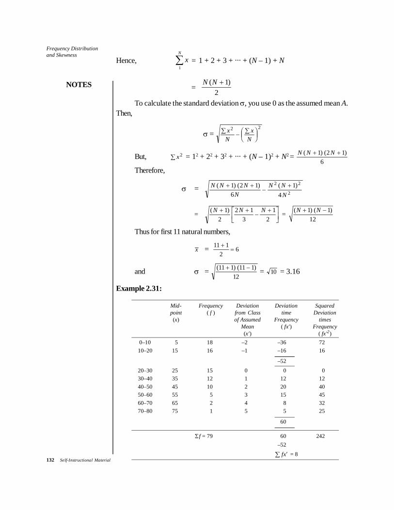
132 Self-Instructional Material
Frequency Distributionand Skewness
NOTES
Hence,1
N
x∑ = 1 + 2 + 3 + ... + (N – 1) + N
= ( 1)
2N N +
To calculate the standard deviation σ, you use 0 as the assumed mean A.Then,
σ = xN
xN
2 2∑ − ∑FHGIKJ
But, x2∑ = 12 + 22 + 32 + ... + (N – 1)2 + N2 = N N N( ) ( )+ +1 2 16
Therefore,
σ = N N NN
N NN
( ) ( ) ( )+ +−
+1 2 16
14
2 2
2
= ( )N N N+ +−
+LNM
OQP
12
2 13
12
= ( 1) ( 1)12
N N+ −
Thus for first 11 natural numbers,
x = 11 12
6+
=
and σ = ( ) ( )11 1 11 112
+ − = 10 = 3.16
Example 2.31:
Mid- Frequency Deviation Deviation Squaredpoint ( f ) from Class time Deviation(x) of Assumed Frequency times
Mean ( fx') Frequency(x') ( fx'2)
0–10 5 18 –2 –36 7210–20 15 16 –1 –16 16
–52
20–30 25 15 0 0 030–40 35 12 1 12 1240–50 45 10 2 20 4050–60 55 5 3 15 4560–70 65 2 4 8 3270–80 75 1 5 5 25
60
Σf = 79 60 242–52
fx ′∑ = 8

Frequency Distributionand Skewness
NOTES
Self-Instructional Material 133
Solution: Since the deviations are from assumed mean and expressed in terms ofclass interval units,
σ = i xN
fxN
× ′∑ −′∑F
HGIKJ
2 2
= 10 24279
879
2× − FHG
IKJ
= 10 × 1.75 = 17.5
Combining standard deviations of two distributionsIf you are given two sets of data of N1 and N2 items with means x1 and x2 andstandard deviations σ1 and σ2 respectively, you can obtain the mean and standarddeviation x and σ of the combined distribution using the following formulae:
x = N x N xN N
1 1 2 2
1 2
++
(2.10)
σ = N N N x x N x x
N N1 1
22 2
21 1
22 2
2
1 2
σ σ+ + − + −
+
( ) ( )(2.11)
Example 2.32: The mean and standard deviations of two distributions of 100and 150 items are 50, 5 and 40, 6 respectively. Find the standard deviation of alltaken together.Solution: Combined mean,
x = N x N xN N
1 1 2 2
1 2
++
= 100 50 150 40100 150× ×+
+= 44
Combined standard deviation,
σ = 2 2 2 2
1 1 2 2 1 1 2 2
1 2
( ) ( )+ + − + −+
N N N x x N x xN N
σ σ
= 100 5 150 6 100 44 50 150 44 40100 150
2 2 2 2× ( ) ( ) ( ) ( )+ + − + −+
= 7.46Example 2.33: A distribution consists of three components with 200, 250, 300items having mean 25, 10 and 15 and standard deviation 3, 4 and 5, respectively.Find the standard deviation of the combined distribution.Solution: In the usual notations, here you have
N1 = 200, N2= 250, N3 = 300
x1 = 25, x2 = 10, x3 = 15

134 Self-Instructional Material
Frequency Distributionand Skewness
NOTES
Formulae (2.6) and (3.7) can easily be extended for combination of threeseries as:
x = N x N x N xN N N
1 1 2 2 3 3
1 2 3
+ ++ +
= 200 25 250 10 300 15200 250 300
× × ×+ ++ +
= 12000750
= 16
and,
σ =
2 2 2 21 1 2 2 3 3 1 1
2 22 2 3 3
1 2 3
( )
( ) ( )
N N N N x x
N x x N x xN N N
σ σ σ+ + + −
+ − + −+ +
= 200 9 250 16 300 25 200 81 250 36 300 1200 250 300
× × × × × ×+ + + + ++ +
= 51 73 7 19. .=
2.5.4 Merits, Limitations and Characteristics of MeasuresThe range is the easiest to calculate the measure of dispersion, but since it dependson extreme values, it is extremely sensitive to the size of the sample, and to thesample variability. In fact, as the sample size increases, the range increasesdramatically, because the more the items one considers, the more likely it is thatsome item will turn up which is larger than the previous maximum or smaller thanthe previous minimum. So, it is, in general, impossible to interpret properly thesignificance of a given range unless the sample size is constant. It is for this reasonthat there appears to be only one valid application of the range, namely in statisticalquality control where the same sample size is repeatedly used, so that comparisonof ranges is not distorted by differences in sample size.
The quartile deviations and other such positional measures of dispersionsare also easy to calculate. However, they suffer from the disadvantage that theyare not amenable to algebraic treatment. Similarly, the mean deviation is not suitablebecause we cannot obtain the mean deviation of a combined series from thedeviations of component series. However, it is easy to interpret and easier tocalculate than the standard deviation.
The standard deviation of a set of data is one of the most important statisticsdescribing it. It lends itself to rigorous algebraic treatment, is rigidly defined and isbased on all observations. It is, therefore, quite insensitive to sample size (providedthe size is ‘large enough’) and is least affected by sampling variations.
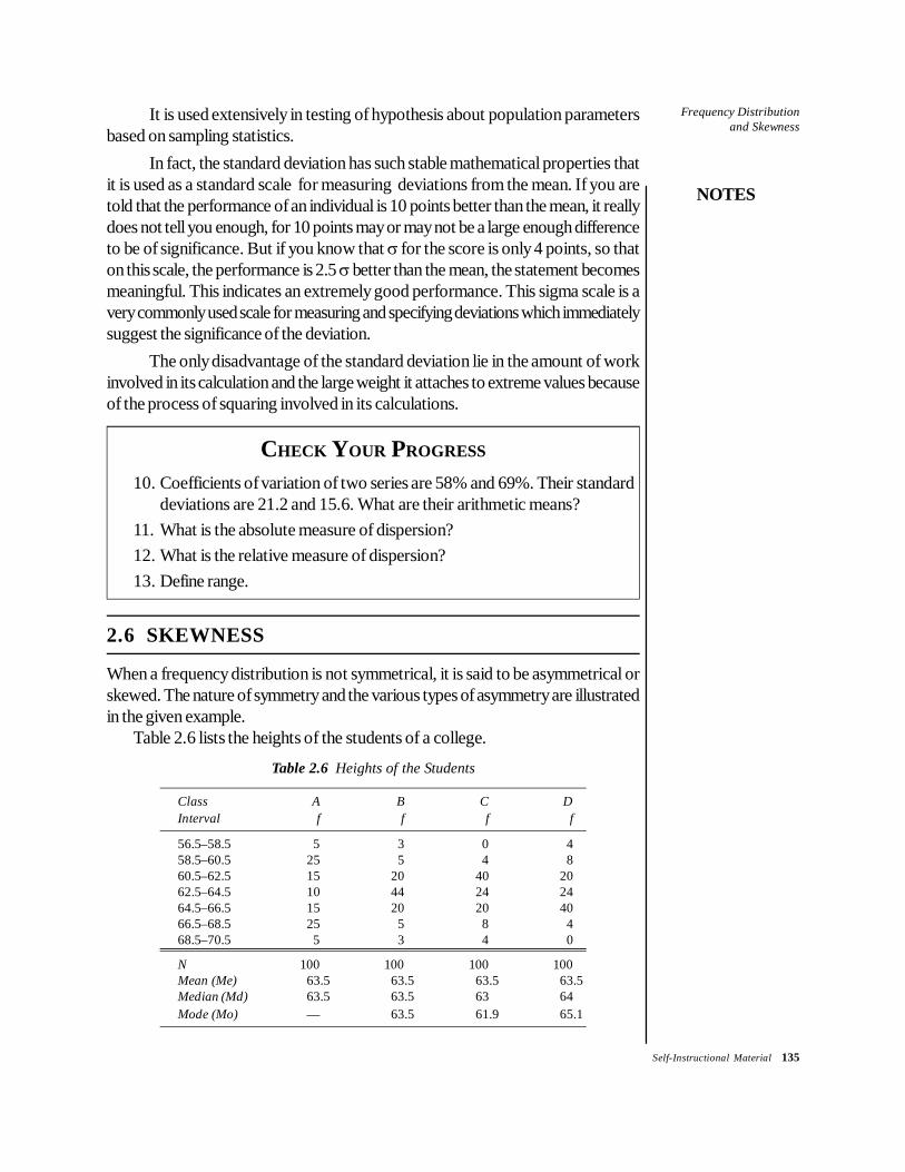
Frequency Distributionand Skewness
NOTES
Self-Instructional Material 135
It is used extensively in testing of hypothesis about population parametersbased on sampling statistics.
In fact, the standard deviation has such stable mathematical properties thatit is used as a standard scale for measuring deviations from the mean. If you aretold that the performance of an individual is 10 points better than the mean, it reallydoes not tell you enough, for 10 points may or may not be a large enough differenceto be of significance. But if you know that σ for the score is only 4 points, so thaton this scale, the performance is 2.5 σ better than the mean, the statement becomesmeaningful. This indicates an extremely good performance. This sigma scale is avery commonly used scale for measuring and specifying deviations which immediatelysuggest the significance of the deviation.
The only disadvantage of the standard deviation lie in the amount of workinvolved in its calculation and the large weight it attaches to extreme values becauseof the process of squaring involved in its calculations.
CHECK YOUR PROGRESS
10. Coefficients of variation of two series are 58% and 69%. Their standarddeviations are 21.2 and 15.6. What are their arithmetic means?
11. What is the absolute measure of dispersion?12. What is the relative measure of dispersion?13. Define range.
2.6 SKEWNESS
When a frequency distribution is not symmetrical, it is said to be asymmetrical orskewed. The nature of symmetry and the various types of asymmetry are illustratedin the given example.
Table 2.6 lists the heights of the students of a college.
Table 2.6 Heights of the Students
Class A B C DInterval f f f f
56.5–58.5 5 3 0 458.5–60.5 25 5 4 860.5–62.5 15 20 40 2062.5–64.5 10 44 24 2464.5–66.5 15 20 20 4066.5–68.5 25 5 8 468.5–70.5 5 3 4 0
N 100 100 100 100Mean (Me) 63.5 63.5 63.5 63.5Median (Md) 63.5 63.5 63 64Mode (Mo) — 63.5 61.9 65.1
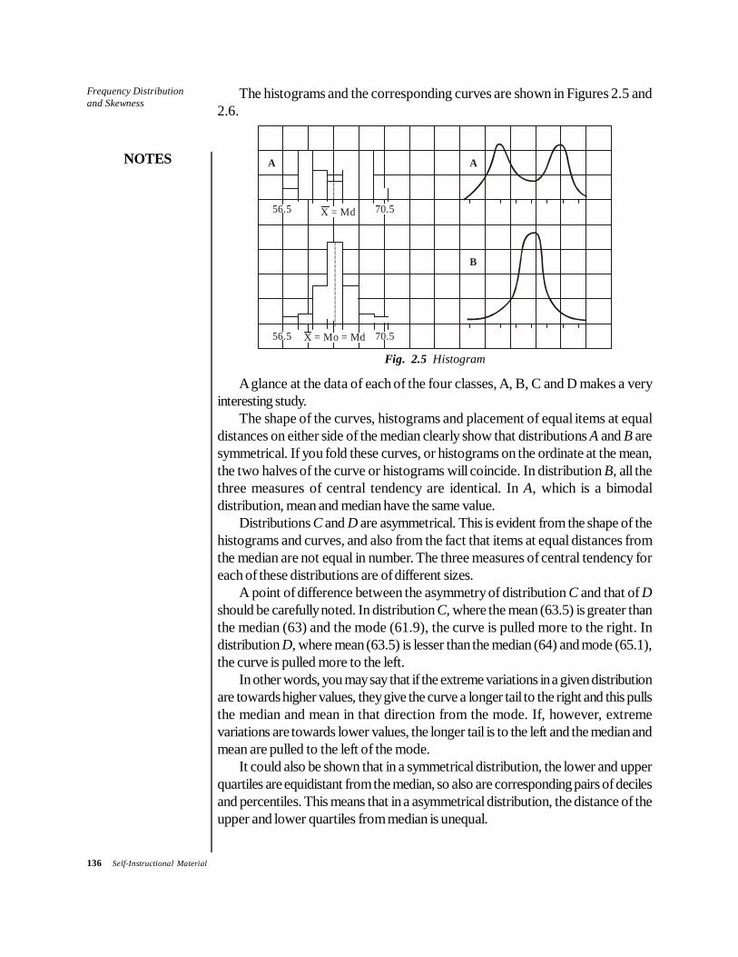
136 Self-Instructional Material
Frequency Distributionand Skewness
NOTES
The histograms and the corresponding curves are shown in Figures 2.5 and2.6.
56.5 X = Mo = Md 70.5
A A
B
56.5 X = Md 70.5
Fig. 2.5 Histogram
A glance at the data of each of the four classes, A, B, C and D makes a veryinteresting study.
The shape of the curves, histograms and placement of equal items at equaldistances on either side of the median clearly show that distributions A and B aresymmetrical. If you fold these curves, or histograms on the ordinate at the mean,the two halves of the curve or histograms will coincide. In distribution B, all thethree measures of central tendency are identical. In A, which is a bimodaldistribution, mean and median have the same value.
Distributions C and D are asymmetrical. This is evident from the shape of thehistograms and curves, and also from the fact that items at equal distances fromthe median are not equal in number. The three measures of central tendency foreach of these distributions are of different sizes.
A point of difference between the asymmetry of distribution C and that of Dshould be carefully noted. In distribution C, where the mean (63.5) is greater thanthe median (63) and the mode (61.9), the curve is pulled more to the right. Indistribution D, where mean (63.5) is lesser than the median (64) and mode (65.1),the curve is pulled more to the left.
In other words, you may say that if the extreme variations in a given distributionare towards higher values, they give the curve a longer tail to the right and this pullsthe median and mean in that direction from the mode. If, however, extremevariations are towards lower values, the longer tail is to the left and the median andmean are pulled to the left of the mode.
It could also be shown that in a symmetrical distribution, the lower and upperquartiles are equidistant from the median, so also are corresponding pairs of decilesand percentiles. This means that in a asymmetrical distribution, the distance of theupper and lower quartiles from median is unequal.

Frequency Distributionand Skewness
NOTES
Self-Instructional Material 137
C C
DD
MEDIANMODE
MEAN
MEDIANMODE
MEAN 70.556.5
70.556.5
Fig. 2.6 Skewness
From the preceding discussion, we can summarize that skewness is present:1. When the graph of the distribution does not show a symmetrical curve.2. When the three measures of central tendency differ from one another.3. When the sum of the positive deviations from the median is not equal to the
negative deviations from the same value.4. When the distances from the median to the quartiles are unequal.5. When corresponding pairs of deciles or percentiles are not equidistant from
the median.
2.6.1 Measures of SkewnessOn the basis of the above tests, the following measures of skewness have beendeveloped:
1. Relationship between three measures of central tendency—commonlyknown as the Karl Pearson’s measure of skewness.
2. Quartile measure of skewness—known as Bowley’s measure of skewness.3. Percentile measure of skewness—also called the Kelly’s measure of
skewness.4. Measures of skewness based on moments.All these measures describe both the direction and the extent of the skewness.
1. Karl Pearson’s measure of skewness
You know that in a perfectly symmetrical distribution, the three measures of centraltendency, namely mean, median and mode will coincide. As the distribution departsfrom symmetry, these three values are pulled apart, the difference between themean and mode being the greatest. Karl Pearson has suggested the use of this
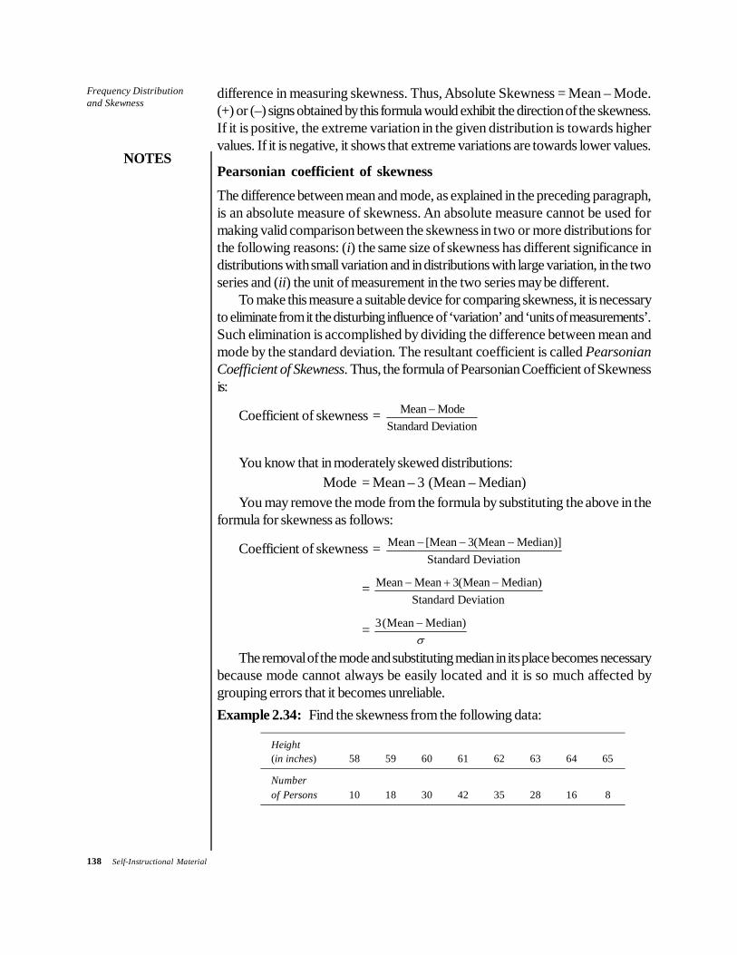
138 Self-Instructional Material
Frequency Distributionand Skewness
NOTES
difference in measuring skewness. Thus, Absolute Skewness = Mean – Mode.(+) or (–) signs obtained by this formula would exhibit the direction of the skewness.If it is positive, the extreme variation in the given distribution is towards highervalues. If it is negative, it shows that extreme variations are towards lower values.
Pearsonian coefficient of skewness
The difference between mean and mode, as explained in the preceding paragraph,is an absolute measure of skewness. An absolute measure cannot be used formaking valid comparison between the skewness in two or more distributions forthe following reasons: (i) the same size of skewness has different significance indistributions with small variation and in distributions with large variation, in the twoseries and (ii) the unit of measurement in the two series may be different.
To make this measure a suitable device for comparing skewness, it is necessaryto eliminate from it the disturbing influence of ‘variation’ and ‘units of measurements’.Such elimination is accomplished by dividing the difference between mean andmode by the standard deviation. The resultant coefficient is called PearsonianCoefficient of Skewness. Thus, the formula of Pearsonian Coefficient of Skewnessis:
Coefficient of skewness = Mean ModeStandard Deviation
−
You know that in moderately skewed distributions:Mode = Mean – 3 (Mean – Median)
You may remove the mode from the formula by substituting the above in theformula for skewness as follows:
Coefficient of skewness = Mean [Mean 3(Mean Median)]Standard Deviation
− − −
= Mean Mean 3(Mean Median)Standard Deviation
− + −
= 3(Mean Median)σ−
The removal of the mode and substituting median in its place becomes necessarybecause mode cannot always be easily located and it is so much affected bygrouping errors that it becomes unreliable.Example 2.34: Find the skewness from the following data:
Height(in inches) 58 59 60 61 62 63 64 65
Numberof Persons 10 18 30 42 35 28 16 8

Frequency Distributionand Skewness
NOTES
Self-Instructional Material 139
Solution: Height is a continuous variable, and hence 58″ must be treated as 57.5″–58.5″, 59″ as 58.5″–59.5″, and so on.
Height Frequency x′ fx′ fx′2 Cumulative(in inches) f from 61 Frequency
58 10 –3 –30 90 1059 18 –2 –36 72 28
59.5″–60–60.5″ 30 –1 –30 30 58–96
60.5″–61–61.5″ 42 0 0 0 100
62 35 1 35 35 13562.5″–63–63.5″ 28 2 56 112 16363.5″–64–64.5″ 16 3 48 144 179
65 8 4 32 128 187
187 171 611
+75
Mean = 61 + 75187
= 61.4, Mode = 60.5 + 3565
= 61.04
σ =2611 75
187 187⎛ ⎞− ⎜ ⎟⎝ ⎠ = 3.27 0.16− = 3.11 = 1.76
Skewness = 61.4 – 61.04 = 0.36 inches.
Coefficient of skewness = 0.361.76
= 0.205
Alternatively, we can determine the median as follows:
Median = The size of 1872
th item = 93.5th item
= 60.5 + 1 35.542
× = 61.35
Skewness = 3(61.4 – 61.35) = 3(0.05) = 0.15
Coefficient of skewness = 0.151.76
= 0.09
The two coefficients are different because of the difficulties associated withdetermination of mode.
2. Bowley’s (Quartile) measure of skewnessIn the above two methods of measuring skewness, the whole series is taken intoconsideration. But, absolute as well as relative skewness may be secured even fora part of the series. The usual device is to measure the distance between the lowerand the upper quartiles. In a symmetrical series, the quartiles would be equidistantfrom the value of the median, i.e.
Median – Q1 = Q3 – Median

140 Self-Instructional Material
Frequency Distributionand Skewness
NOTES
In other words, the value of the median is the mean of Q1 and Q3. In a skeweddistribution, quartiles would not be equidistant from median unless the entireasymmetry is located at the extremes of the series. Bowley has suggested thefollowing formula for measuring skewness, based on the preceding facts.
Absolute SK = (Q3 – Me) – (Me – Q1)= Q3 + Q1 – 2 Me (2.12)
If the quartiles are equidistant from the median, i.e. (Q3 – Md) = (Md – Q1),then SK = 0. If the distance from the median to Q1 exceeds that from Q3 to themedian, this will give a negative skewness. If the reverse is the case, it will give apositive skewness.
If the series expressed in different units are to be compared, it is essential toconvert the absolute amount into the relative. Using the interquartile range as adenominator we have for the coefficient of skewness as follows:
Relative SK = 3 1
3 1
2MdQ QQ Q+ −
− (2.13)
or, 3 1
3 1
( Md) (Md )( Md) (Md )Q QQ Q
− − −− + −
If in the series the median and lower quartiles coincide, then the SK becomes(+1). If the median and upper quartiles coincide, then the SK becomes (–1).
This measure of skewness is rigidly defined and easily computable. Further,such a measure of skewness has the advantage that it has value limits between(+1) and (–1), with the result that it is sufficiently sensitive for many requirements.The only criticism levelled against such a measure is that it does not take intoconsideration all the items of these series, i.e. extreme items are neglected.Example 2.35: Calculate the coefficient of skewness of the data of table given inExample 2.34 based on quartiles.Solution: With reference to table given in Example 2.34, you have
Q1 = The size of 187th 46.75th item4 4N ⎛ ⎞= =⎜ ⎟⎝ ⎠
= 59.5 + 18.7530
= 59.5 + 0.63 = 60.13
Q3 = The size of 3 3 187th item 140.25th item4 4N ×⎛ ⎞= =⎜ ⎟⎝ ⎠
= 62.5 + 5.2528
= 62.5 + 0.19 = 62.69Skewness = 62.69 + 60.13 – 2 (61.35) = 0.12
(using formula 2.12)

Frequency Distributionand Skewness
NOTES
Self-Instructional Material 141
Coefficient of skewness = 0.12
62.69 60.13−(using formula 2.13)
= 0.122.56
= 0.047
3. Kelly’s (Percentile) measure of skewnessTo remove the defect of Bowley’s measure that it does not take into account allthe values, it can be enlarged by taking two deciles (or percentiles), equidistantfrom the median value. Kelly has suggested the following measure of skewness:
SK = P50 – 90 102
P P+
= D5 – 9 12
D D+
Though such a measure has got little practical use, yet theoretically this measureseems very sound.
Example 2.36: Calculate the Karl Pearson’s coefficient of skewness from thefollowing data:
Marks No. of Students Marks No. of Students
above 0 150 above 50 70” 10 140 ” 60 30” 20 100 ” 70 14” 30 80 ” 80 0” 40 80
Solution:
Marks Frequency Midpoint X = (X – A)/10 f(X′) f(X′2) CumulativeFrequency (cf)
0–10 10 5 –3 –30 90 1010–20 40 15 –2 –80 160 5020–30 20 25 –1 –20 20 70
–130
30–40 0 35 0 0 0 7040–50 10 45 1 10 10 8050–60 40 55 2 80 160 12060–70 16 65 3 48 144 13670–80 14 75 4 56 224 150
150 194 808
+64
Since it is a bimodal distribution Karl Pearson coefficient is appropriate andwe need to calculate X , Me and σ.
X = 35 + 64150
× 10 = 35 + 4.27 = 39.27

142 Self-Instructional Material
Frequency Distributionand Skewness
NOTES
Median = Size of 1502
th item
= 40 + 10 510× = 45
Standard deviation (σ) = i × 22( ) ( )f X f X
N NΣ Σ′ ′⎛ ⎞− ⎜ ⎟⎝ ⎠
=2808 6410
150 150⎛ ⎞× − ⎜ ⎟⎝ ⎠
= 10 5.387 0.182× −
= 10 × 2.28 = 22.8
Skewness = 3( Median)X −σ
= 3(39.27 45)22.8
−
= 3( 5.73)22.8− = 17.19
22.8− = – 0.75
Example 2.37: From the following data compute quartile deviation and thecoefficient of skewness.
Size 5–7 8–10 11–13 14–16 17–19Frequency 14 24 38 20 4
Solution:
Size Frequency Cumulative Frequency
4.5–7.5 14 147.5–10.5 24 38
10.5–13.5 38 7613.5–16.5 20 9616.5–19.5 4 100
Q1 = 7.5 + 3 1124× = 8.87
Q3 = 10.5 + 3 3738× = 10.5 + 111
38 = 10.5 + 2.92 = 13.42
Median = 10.5 + 3 1238× = 10.5 + 36
38 = 10.5 + 0.947 = 11.447
Quartile deviation = 3 12
Q Q− = 13.42 8.872− = 4.55
2 = 2.275

Frequency Distributionand Skewness
NOTES
Self-Instructional Material 143
Skewness = 3 1
3 1
2MeQ QQ Q+ −
−
= 13.42 8.87 22.8913.42 8.87
+ −−
= 0.64.55− = – 0.13
Example 2.38: In a certain distribution the following results were obtained:
X = 45.00; Median = 48.00Coefficient of Skewness = – 0.4
You are required to estimate the value of standard deviation.Solution:
Skewness = 3 (Mean Median)σ−
– 0.4 = 3 (45 48)σ−
– 0.4σ = – 9
σ = 90.4
= 22.5
Example 2.39: Karl Pearson’s coefficient of skewness of a distribution is +0.32.Its standard deviation is 6.5 and mean is 29.6. Find the mode and median of thedistribution.Solution:
Coefficient of skewness= Mean Modeσ−
0.32 = 29.6 Mode6.5−
or 6.5 × 0.32 = 29.6 – ModeMode = 29.6 – 2.08 = 27.52
Coefficient of skewness= 3 (Mean Median)σ−
0.32 = 3(29.6 Median)6.5−
6.5 × 0.32 = 88.8 – 3 Median
Median = 88.8 2.083− = 28.91
Example 2.40: You are given the position in a factory before and after thesettlement of an industrial dispute. Comment on the gains or losses from the pointof the workers and that of the management.

144 Self-Instructional Material
Frequency Distributionand Skewness
NOTES
Before AfterNo. of Workers 2440 2359Mean Wages 45.5 47.5Median Wages 49.0 45.0Standard Deviation 12.0 10.0
Solution:Employment. Since the number of workers employed after the settlement is lessthan the number of employed before, it has gone against the interest of the workers.
Wages. The total wages paid after the settlement were 2350 × 47.5 = Rs1,11,625; before the settlement the amount disbursed was 2400 × 45.5 = Rs1,09,200.
This means that the workers as a group are better off now than before thesettlement, and unless the productivity of workers has gone up, this may be againstthe interest of management.
Uniformity in the wage structure. The extent of relative uniformity in thewage structure before and after the settlement can be determined by a comparisonof the coefficient of variation.
Coefficient of variation, before = 1245.5
× 100 = 26.4
Coefficient of variation, after = 1047.5
× 100 = 21.05
This clearly means that there is comparatively lesser disparity in due wagesreceived by the workers. Such a position is good for both the workers and themanagement.
Pattern of the wage structure. A comparison of the mean with the medianleads to the obvious conclusion that before the settlement more than 50 per centof the workers were getting a wage higher than this mean, i.e. (Rs. 45.5). After thesettlement the number of workers whose wages were more than Rs. 45.5 becameless than 50 per cent. This means that the settlement has not been beneficial to allthe workers. It is only 50 per cent workers who have been benefited as a result ofan increase in the total wages bill.
CHECK YOUR PROGRESS
14. What is skewness?15. Name the measures of skewnness.
2.7 SUMMARY
In this unit, you have learned that:• The most important objective of statistical analysis is to determine a single
value for the entire mass of data so that it describes the overall level of the

Frequency Distributionand Skewness
NOTES
Self-Instructional Material 145
group of observations and can be considered a representative value of thewhole set of data.
• Variance or coefficient of variation has the same properties as standarddeviation and is the square of standard deviation, represented as σ2.
• The measure of dispersion is an important property of a distribution andneeds to be measured by appropriate statistics.
• The measure of dispersion describes absolute and relative measures ofdispersion. In its absolute form, it states the actual amount by which thevalue of an item on average deviates from a measure of central tendency.
• Absolute measures are expressed in concrete units, i.e. units in terms ofwhich the data have been expressed, e.g. rupees, centimetres, kilograms,etc., and are used to describe frequency distribution.
• A relative measure of dispersion is a quotient obtained by dividing theabsolute measures by a quantity in respect of which absolute deviation hasbeen computed. It is as such a pure number and is usually expressed in apercentage form.
• Relative measures are used for making comparisons between two or moredistributions.
• Skewness refers to lack of symmetry in distribution.
2.8 KEY TERMS
• Mean: It is basically an arithmetic average and is the measure of centrallocation.
• Mode: It is also a form of average and can be defined as the most frequentlyoccurring value in the data.
• Median: It is a measure of central tendency and it appears in the centre ofan ordered data.
• Quartile: It divides the data into four equal parts.• Deciles: It divides the total ordered data into ten equal parts.• Percentile: It divides the data into hundred equal parts.• Variance: It is the square of standard deviation, represented as σ2, and has
the same properties as standard deviation.• Range: It is the difference between the maximum and minimum values of a
set of numbers. It indicates the limits within which the values fall.• Quartile deviation: This deviation refers to a type of range based on the
quartiles.• Mean deviation: It is the arithmetic mean of the absolute deviations of a
series of values.

146 Self-Instructional Material
Frequency Distributionand Skewness
NOTES
• Standard deviation: It is the measure of the dispersion of a set of valuesand is calculated from the mean of squared deviations.
• Skewness: It is a measure of asymmetry of the distribution of a real-valuedrandom variable. A skew can be positive or negative.
2.9 ANSWERS TO ‘CHECK YOUR PROGRESS’
1. A variable is considered as continuous when it can assume an infinite numberof real values and it is considered discrete when it is the finite number of realvalues.
2. When the interest of the investigator focuses on the number of items belowa specified value, then this specified value is the upper limit of the classinterval. It is known as less than cumulative frequency distribution.
3. A single number describing some feature of a frequency distribution is calleddescriptive statistics.
4. The arithmetic mean is also commonly known as simply the mean. Eventhough average, in general, means any measure of central location. Whenwe use the word average in our daily routine, we always mean the arithmeticaverage.
5. The advantages of mean are as follows:• It is a measure that can be easily calculated.• It includes all values of the data set in its calculation.• Its value varies very little from sample to sample taken from the same
population.• It is useful for performing statistical procedures such as computing and
comparing the means of several data sets.6. Mean = 68
Mode = 80Median = 72
7. Mean = 78. Rs 162.19. 98
10. 36.6 approx. and 22.6 approx.11. The absolute measure of dispersion states the actual amount by which an
item on average deviates from a measure of central tendency.12. The relative measure of dispersion is a quotient computed by dividing the
absolute measures by a quantity in respect of which the absolute deviationhas been computed.

Frequency Distributionand Skewness
NOTES
Self-Instructional Material 147
13. The range of a set of numbers is the difference between the maximum andminimum values. It indicates the limits within which the values fall.
14. Skewness refers to the lack of symmetry in a distribution. In the symmetricaldistribution, the mean, median and mode coincide.
15. The following are the measures of skewness:• Relationship between three measures of central tendency—commonly
known as the Karl Pearson’s measure of skewness• Quartile measure of skewness—known as Bowley’s measure of
skewness• Percentile measure of skewness—also called the Kelly’s measure of
skewness• Measures of skewness based on moments
2.10 QUESTIONS AND EXERCISES
Short-Answer Questions
1. What do you understand by frequency distribution?2. How would you convert discrete data into continuous data?3. What do you mean by descriptive statistics?4. How is central tendency measured?5. Define the term arithmetic mean.6. Write three characteristics of mean.7. What is the importance of arithmetic mean in statistics?8. Explain the term median with example.9. How is location of median calculated using graphic analysis?
10. Define quartiles, deciles and percentiles with suitable examples.11. What is the coefficient of variation?12. What is range? How is it measured?13. Write the definition and formula of quartile deviation.14. How will you calculate the mean deviation of given data?15. Explain standard deviation. Why is it used in statistical evaluation of data?16. Calculate standard deviation for the series 1, 2, 3, 5, 7.17. For a group of 50 male workers the mean and standard deviation of their
weekly wages are Rs 63 and Rs 9 respectively. For a group of 40 femaleworkers these are Rs 54 and Rs 6 respectively. Find the standard deviationof the combined group of 90 workers.

148 Self-Instructional Material
Frequency Distributionand Skewness
NOTES
18. (a) Mean and standard deviations of two distributions of 100 and 150items are 50, 5 and 40, 6 respectively. Find the mean and standarddeviations of all the 250 items taken together.
(b) Mean and standard deviations of 100 items are found by a student as9 and if at the time of calculations two items are wrongly taken as 40and 50 instead of 60 and 30, find the correct mean and standarddeviations.
19. How will you measure skewness?
Long-Answer Questions
1. Explain the guidelines to be considered in constructing a frequencydistribution.
2. Define the various measures of central tendency. What purposes do theirmeasurement serve?
3. Define geometric and harmonic mean and explain their uses.4. Show the relative positions of different averages in a moderately symmetrical
series.5. What do you mean by the following:
(a) Quartiles(b) Deciles(c) Percentiles
6. What are the qualities which an average must possess? Which of the averagespossess most of these qualities?
7. What do you mean by ‘weights’? Why are they assigned? Point out a fewcases in which weighted average should be used.
8. Differentiate between crude and corrected death rates.9. The expenditure of ten families in rupees are given below:
Family A B C D E F G H I JExpenditure 30 70 10 75 500 8 52 250 50 36Calculate the arithmetic average by (a) direct method and (b) short-cutmethod.
10. Calculate mean deviation and its coefficient about median, arithmetic meanand mode for the following figures, and show that the mean deviation aboutthe median is the least.103, 50, 68, 110, 108, 105, 174, 103, 150, 200, 225, 350, 103

Frequency Distributionand Skewness
NOTES
Self-Instructional Material 149
11. Compute mean deviations of the two series and point out which is morevariable.
Month Index No. Index No. Month Index No. Index No.Calcutta Delhi Calcutta Delhi
1970 April 93 107 1970 October 97 1071970 May 97 108 1970 November 97 1051970 June 95 102 1970 December 92 1011970 July 95 102 1971 January 93 1001970 August 95 102 1971 February 89 97
1970 September 95 104 1971 March 89 96
12. Calculate (a) median coefficient of dispersion and (b) mean coefficient ofdispersion from the following data:Size of Items 14 16 18 20 22 24 26Frequency 2 4 5 3 2 1 4
13. Compute the mean deviation from the median and from the mean for thefollowing distribution of the scores of 50 college students. Also completethe class interval.Scores 140– 150– 160– 170– 180– 190–200Frequency 4 6 10 18 9 3
14. Find the mean deviation about the mean of the following data of ages ofmarried men in a certain town.Ages 15–24 25–34 35–44 45–54 55–64 65–74No. of Men 33 264 303 214 128 58
15. Calculate the mean deviation from the following data. What light does itthrow on the social conditions of the community?Difference in age between husband and wife:Difference
in Years: 0–5 5–10 10–15 15–20 20–25 25–30 30–35 35–40Frequency: 449 705 507 281 109 52 16 4
16. The following figures give the income of 10 persons in rupees. Find thestandard deviation.
114, 115, 123, 120, 110, 130, 119, 118, 116, 11517. Calculate the mean and standard deviation of the following values of the
world’s annual gold output in millions of pound (for 20 different years)94, 95, 96, 93, 87, 79, 73, 69, 68, 67, 78, 82, 83, 89, 95, 103, 108, 117,130, 97.Also calculate the percentage of cases lying outside the mean at distances±σ, ±2σ, ±3σ where σ denotes the standard deviation.

150 Self-Instructional Material
Frequency Distributionand Skewness
NOTES
18. Calculate standard deviation from the following data:Size of Item 6 7 8 9 10 11 12Frequency 3 6 9 13 8 5 4
19. Calculate the arithmetic mean and the standard deviation from the followingdata:Class Interval 5–10 10–15 15–20 20–25 25–30 30–35 35–40 40–45Frequency 6 5 15 10 5 4 3 2
20. Calculate the mean and the standard deviations from the following data:Age Group 20–25 25–30 30–35 35–40 40–45 45–50 50–55 55 and
Below aboveNo. of 26 44 60 101 109 846 66 10
Employees21. Calculate mean and standard deviation from the following data:
Age Under 10 20 30 40 50 60 70 80No. of Persons Dying 15 30 53 75 100 110 115 125
22. The marks obtained by the students of class A and B are given below:Marks 5–10 10–15 15–20 20–25 25–30 30–35 35–40 40–45Class A 1 10 20 8 6 3 1 –Class B 5 6 15 10 5 4 2 2Calculate mean, median, mode and standard deviation for the distributions.Explain your results regarding composition of the class in respect ofintelligence.
23. Explain clearly the ideas implied in using arbitrary working origin and scalefor the calculation of the arithmetic mean and standard deviation of frequencydistribution.The values of arithmetic mean and standard deviation of the followingfrequency distribution of a continuous variable derived from analysis areRs 135.33 and Rs 9.6 respectively. Find the upper and lower limits of thevarious classes:
X' –4 –3 –2 –1 0 +1 +2 +3f 2 5 8 18 22 13 8 4
24. (a) Mean of 100 items is 50 and their standard deviation is 4. Find thesum and sum of squares of all the items.
(b) The mean and the standard deviation of a sample of 100 observationswere calculated as 40 and 5.1, respectively, by a student, who tookby mistake 50 instead of 40 for one observation. Calculate the correctmean and standard deviation.

Frequency Distributionand Skewness
NOTES
Self-Instructional Material 151
25. The following data give the arithmetic averages and standard deviations ofthe three subgroups. Calculate the arithmetic average and standard deviationof the whole group.
Subgroup No. of Men Average SD ofWage (Rs) Wage (Rs)
A 50 61.0 8.0B 100 70.0 9.0C 120 80.5 10.0
26. For a group containing 100 observations, the arithmetic mean and standarddeviation are 8 and 10 5. respectively. For 50 observations selected fromthese 100 observations the mean and the standard deviation are 10 and 2respectively. Find the arithmetic mean and the standard deviation of theother half.
27. A group has σ = 10, N = 60, σ2 = 4. A subgroup of this has X1 = 11,N1 = 40, σ1
2 = 2.25. Find the mean and standard deviation of the othersubgroup.
28. Two cricketers scored the following runs in the several innings. Find who isa better run-getter and who is a more consistent player.A 42, 17, 83, 59, 72, 76, 64, 45, 40, 32B 28, 70, 31, 0, 59, 108, 82, 14, 3, 95
29. The following are some of the particulars of the distribution of weights ofboys and girls in a class.
Boys GirlsNumber 100 50Mean weight (kg) 60 45Variance 9 4
(a) Find standard deviation of the combined data.(b) Which of the two distributions is more variable?
2.11 FURTHER READING
Anderson, David R., Dennis J. Sweeney and Thomas A. Williams. Essentials ofStatistics for Business and Economics. Mumbai: Thomson Learning, 2007.
Anderson, David R., Dennis J. Sweeney and Thomas A. Williams. QuantitativeMethods for Business. Mumbai: Thomson Learning, 2005.
Bhardwaj, R.S. Business Statistics. New Delhi: Excel Books, 2000.Chandan, J.S. Business Statistics. New Delhi: Vikas Publishing House, 2004.Gupta, C.B. and Vijay Gupta. An Introduction to Statistical Methods.
New Delhi: Vikas Publishing House, 2004.

152 Self-Instructional Material
Frequency Distributionand Skewness
NOTES
Hooda. R.P. Statistics for Business & Economics. New Delhi: Macmillan IndiaLtd., 2004.
Kothari C.R. Quantitative Techniques. New Delhi: Vikas Publishing House,1984.
Levin, Richard I. and David S. Rubin. Statistics for Business. New Delhi: PrenticeHall of India, 1990.
Monga, G.S. Mathematics and Statistics for Economics. New Delhi: VikasPublishing House.
Sancheti D.C. and V.K. Kapoor. Business Mathematics. New Delhi: Sultan Chand& Sons.
Zameeruddin Qazi, V.K. Sharma and S.K. Bhambri. Business Mathematics.New Delhi: Vikas Publishing House, 2008.

First Published: 2009
Copyright © 2009, Excel Books, Private Limited
All Rights Reserved Produced & Printed
by
EXCEL BOOKS PRIVATE LIMITED A-45, Naraina Industrial Area, Phase-1
New Delhi-110028
for
UBS | THE SAMPURAN PRAKASH SCHOOL OF EXECUTIVE EDUCATION Gurgaon, Haryana, India
www.ubs.edu.in