unintended consequences of price controls: an application

Munich Personal RePEc Archive

Unintended Consequences of Price

Controls: An Application to Allowance

Markets

Stocking, Andrew

Congressional Budget Office

September 2010

Online at https://mpra.ub.uni-muenchen.de/25559/

MPRA Paper No. 25559, posted 04 Oct 2010 21:09 UTC

Working Paper Series


Washington, D.C.

UNINTENDED CONSEQUENCES OF PRICE CONTROLS:

AN APPLICATION TO ALLOWANCE MARKETS

Andrew Stocking

([email protected])

Microeconomic Studies Division


Washington, D.C.

September 2010

Working Paper 2010-06

Working papers in this series are preliminary and are circulated to stimulate discussion and critical comment. These papers are not subject to CBO’s formal review and editing processes. The analysis and conclusions expressed in them are those of the author and should not be interpreted as those of the Congressional Budget Office. References in publications should be cleared with the author. Papers in this series can be obtained at www.cbo.gov/publications (select Working and Technical Papers). This paper benefited from comments by and conversations with Dallas Burtraw, Terry Dinan, Harrison Fell, Sasha Golub, Janet Holtzblatt, Nathaniel Keohane, Joseph Kile, Deborah Lucas, David Moore, Adele Morris, Kevin Perese, Cedric Philibert, Stephen Salant, and one anonymous reviewer. Special thanks to Bob Shackleton and Brian Prest for constructing the sector-specific elasticities.

Abstract

Price controls established in an emissions allowance market to constrain allowance prices

between a ceiling and a floor offer a mechanism to reduce cost uncertainty in a cap-and-trade

program; however, they could provide opportunities for strategic actions by firms that

would result in lower government revenue and greater emissions than in the absence of controls.

In particular, when the ceiling price is supported by introducing new allowances into the market,

firms could choose to buy allowances at the ceiling price, regardless of the prevailing market

price, in order to lower the equilibrium price of all allowances. Those purchases could either be

transacted by a group of firms intending to manipulate the market or be induced through the

introduction of inaccurate information about the cost of emissions abatement that causes firms to

purchase allowances at the ceiling. Theory and simulations using estimates of the elasticity of

allowance demand for U.S. firms suggest that the manipulation could be profitable under the

stylized setting and assumptions evaluated in the paper, although in practice many other

conditions will determine its use.

I. Introduction

In light of growing concern about global climate change, some countries, including the

United States, Australia, and New Zealand, are considering establishing a cap-and-trade

program, similar to that already enacted in the European Union and 10 states in the northeastern

United States, to reduce emissions of carbon dioxide and other greenhouse gases (GHG). Under

such a program, the government would set a limit, or cap, on total GHG emissions (measured as

carbon dioxide-equivalent emissions, or CO2e, which is the amount of emissions of carbon

dioxide alone that would cause an equivalent amount of global warming) and would require

regulated entities, such as oil refiners, natural gas distributors, large electricity generators, and

chemical companies, to hold rights, or allowances, for their emissions. After allowances were

initially distributed, entities could buy and sell them and would be required each year to submit a

number of allowances equal to their CO2e emissions from the previous year. The cost of those

allowances and the cost of eliminating emissions in excess of those allowances represent the cost

of complying with the cap-and-trade program.

Allowance prices under such a program would change from day to day in response to

changes in expectations about the marginal cost of reducing emissions and the demand for

emissions-intensive goods and services. In the face of such uncertainty about compliance costs,

some have proposed placing controls on allowance prices in the form of a maximum price,

sometimes called a price ceiling or safety valve price, and a minimum price, or price floor.1 Such

controls, proponents argue, would achieve a policy goal of trading off the economic costs with

the environmental goals of a cap-and-trade program, and several economists have even

concluded that such controls would only minimally affect the emissions objective of the

program.2

That research, however, implicitly assumes that market participants will not use the price-

control mechanism to influence the price of allowances. The research presented here illustrates

conditions under which participants could lower their cost of compliance with a cap-and-trade

program by weakening the cap, thus reducing the environmental benefits of the program. That

finding relies on the assumption that the cap-and-trade program would adopt a price-control

mechanism similar to that found in most U.S. proposals: it would maintain the price ceiling

through the release of additional allowances into the market when the allowance price threatens

to exceed the ceiling price, but would not preclude such a release any time market participants

are willing to pay the ceiling price for allowances, and would not include an equivalent

mechanism for retracting those allowances should allowance prices later fall. That means that

any release of additional allowances would permanently relax the allowance cap, regardless of

the long-term marginal costs of emissions abatement. Thus, if one or more market participants

were to purchase allowances at the ceiling price, whatever the actual equilibrium price, they

would be lowering the equilibrium price for all allowances, thereby providing a public good to

themselves and other regulated entities by lowering the cost of all allowances.

The provision of that public good – described throughout this paper as a manipulation –

is a possible unintended consequence of price controls not discussed elsewhere in the literature.

The analysis in this paper thus complements research on price manipulation in general and on

manipulation specific to allowance markets by monopsonist buyers.3 The unintended

consequence may not conform to every reader’s definition of manipulation, because it relies on a

natural market response to price controls implemented as described in many cap-and-trade

proposals. In addition, the manipulation does not adversely affect other market participants, as

many market manipulation strategies do, but instead leaves taxpayers worse off through lower

government revenue and reduced environmental benefit. As a result, neither the legality of the

manipulation nor the response of regulators is obvious, and for that reason this paper remains

agnostic on any regulatory response or costs incurred by participants to avoid a regulatory

response.

The next section describes the unintended consequences that would appear to often

accompany price controls, most of which were not predicted before their implementation.

Section III describes a hypothetical U.S. cap-and-trade program and explains qualitatively how

the manipulation of price controls may be one such unintended consequence of such controls in a

cap-and-trade market. Section IV brings theory to that explanation, and Section V describes

some of the key parameters defining the feasibility of the manipulation within the hypothetical

program. Section VI uses those parameter estimates to describe the payoffs of the potential

manipulation and further characterize the manipulation from the perspective of market

participants. Section VII concludes.

II. Historical Use of Price Controls

Many economists believe that a tax is the most efficient mechanism to regulate GHG

emissions. And some point out that a cap-and-trade program that includes price controls could

mimic a tax by limiting the economic costs of a policy to reduce emissions. Furthermore, some

suggest that because the cap-and-trade program would be created through a government policy, it

might operate differently than other markets, for example, energy and agricultural commodity

markets. However, like price controls or price stabilization policies used in other markets, price

controls in allowance markets may have unintended and detrimental consequences. In other

markets, those various consequences tend to be largely unforeseen when the price controls are

introduced. The unintended consequences of price controls in an emissions allowance market

may or may not be similarly unpredictable.

Generally, price controls can be implemented in one of two ways: regulation or supply

management. The regulatory approach simply prohibits any buying or selling at prices above a

maximum price or below a minimum price. Alternatively, controlling prices with supply

management requires the market overseer – in many cases a government entity – to adjust the

supply of the price-controlled commodity to eliminate excess supply in the case of a price floor

and eliminate excess demand in the case of a price ceiling.

Common examples of regulatory price controls include rent controls, which limit the

rental rate a housing owner can charge renters, and the minimum wage, which places a floor on

what an employer can pay employees. It is well established that price controls can create

inefficiencies in the marketplace, for example, by preventing housing from being allocated to

those willing to pay the most for it, or preventing jobs from being allocated to those willing to

work for the lowest wage. But price controls can also have unintended consequences that are

indirectly related to the consumption of the controlled good. For example, in the early 1970s the

U.S. government placed a maximum price on crude oil. Although intended to dampen the

exposure of U.S. consumers to rising energy prices, those price controls created immediate

gasoline shortages and are thought to have created disincentives to produce oil domestically,

which ultimately contributed to a long-term reliance on foreign oil.4

Regulatory price controls are also present in markets with active trading, which may offer

market participants opportunities to capitalize on any inefficiency created by the controls. Most

deregulated electricity markets in the United States currently have a price ceiling set at $1,000

per megawatt-hour (MWhr), far above the typical price of between $30 and $100 per MWhr.5 At

that price, typically reached 10-20 hours each year, the market overseer (called the independent

systems operator) of each regional electricity grid intervenes to clear the market by deciding

which firms will produce electricity, which firms will receive that electricity, and the price at

which they will both transact. The infrequency with which those price ceilings are reached

minimizes any negative consequences of such intervention. Other price controls in electricity

markets, however, have proved less benign. For example, when the California electricity market

was deregulated in the 1990s, that deregulation applied only to the price at which electricity

distributors could purchase electricity on the open market. California retained a regulatory price

ceiling for consumers, with the result that distributors were forced to purchase electricity at

market prices but could pass on only a fraction of those costs (about $60 per MWhr) to

California consumers. That discrepancy between the price at which distributors had to purchase

electricity and the price at which they could sell electricity created an opportunity for some

market participants, such as Enron, to manipulate the market for their own profit. Although the

opportunities for manipulation created by the price controls were not the sole cause of the

California energy crisis, they are generally recognized as a contributing factor.6

Supply management, the second mechanism for controlling prices, has been used by the

U.S. government at various times over the past century to stabilize prices of gold, tin, and silver.

That type of price control requires the market overseer to have either a sufficiently large stock of

the commodity to satisfy excess demand or a cash reserve with which to purchase excess supply.

If excess demand or supply remains after the overseer’s resources are exhausted, the market

price will rise above the price ceiling or fall below the price floor.

In theory, price controls implemented through supply management should have a

stabilizing effect on the price, assuming the intention to implement and enforce the controls is

credible to the market.7 Perfect credibility, however, requires that the market overseer possess an

inexhaustible supply of the commodity or cash. Without such credibility, as would be the case if

the government lacks the resources or authority to support a particular price under any

circumstance, market participants anticipating the reserve’s imminent exhaustion would be

expected to engage in a speculative attack on the price-controlled commodity. To do so, they

would buy the controlled item at the ceiling price to build their own supply and exhaust the

government’s, and then, sell to the market when the price rises above the ceiling.8 In a cap-and-

trade setting, a speculative attack would not be expected to occur if the government had the

authority to print an unlimited number of additional allowances, as some proposals have allowed.

A price floor can also invite a speculative attack. For example, when the United Kingdom

decided in 1990 to join the European Exchange Rate Mechanism (ERM), it had to guarantee that

the pound’s valuation would fluctuate by no more than 6 percent relative to other member

country currencies. In September 1992 both domestic and international pressures pushed the

pound toward the lower bound of that range. In an effort to increase the value of the pound, the

U.K. government sought to reduce supply by purchasing billions of pounds and repeatedly

raising interest rates. Despite this, currency traders sold the pound short, in effect betting that the

government would fail to maintain the price floor. The government ultimately withdrew from the

ERM and allowed the pound to decline in value, generating billions in profits for those currency

traders who had sold the pound short at the government-supported floor.9 A similar speculative

attack occurred in 1985 when the International Tin Council failed in its effort to maintain a tin

price floor.10

Finally, price controls have also been observed to have behavioral implications for

market participants. For example, the behavioral economics literature finds evidence that the

presence of price floors and ceilings causes participants in a laboratory to migrate toward those

price boundaries, as if they provided significant information about the value of the commodity in

question.11 Another strain of economics research provides evidence that price ceilings serve as a

focal point for tacit collusion among producers. Research suggests that the credit card industry in

the 1980s may have used state-specific interest rate ceilings as a focal point for setting interest

rates, which then served as stable equilibrium rates even in the presence of competition that

should have forced rates lower. As a result, the price ceiling may have actually raised consumer

prices for credit card debt.12 Other behavioral reactions to price controls were observed during

the U.S. government’s attempt to apply controls to the gold market in the 1960s.13 In that episode

the government had a strategic reserve of gold that it could use to increase the supply and thus

reduce gold prices if it felt that prices were too high. However, the government did not stipulate

conditions under which it might release gold from that reserve. The resulting uncertainty is

credited with causing consumers and producers of gold to require a higher return for their gold

holdings, which in turn caused the price of gold to increase at a faster rate than it would have

otherwise.

III. Manipulating Price Controls in the Emissions Allowance Market

Proposals in the United States for implementing price controls in a cap-and-trade

emissions allowance market vary, but all rely on the U.S. government’s ability to adjust the

supply of allowances to keep the equilibrium price between the ceiling and floor. Many recent

proposals would control prices by establishing a minimum price at which market participants can

purchase allowances from the government, and a maximum price through the use of either a

limited or an unlimited reserve of additional allowances. The details of their execution vary, but

in most such proposals the reserve is intended to offer market participants an opportunity to

purchase additional allowances at a fixed ceiling price should there be excess demand at that

price. For expositional simplicity, this paper will assume that participants can purchase those

allowances at the ceiling price at their convenience—that is, whether or not the ceiling price is

binding—and that the reserve is sufficiently large to support the demand described in this paper

at the price ceiling. That does not mean the reserve would need to be infinitely large, although it

could be, but only that it represent a sizeable fraction of the annual cap relative to the economy’s

responsiveness to changes in allowance prices (in practice, this could mean the reserve would be

5 to 20 percent of any one year’s issued allowances).

The efficacy of such a price ceiling design rests on the assumption that market

participants will not purchase allowances from the reserve if the allowance price does not

warrant such purchases. But the presence of the ceiling and the implications associated with the

permanent relaxation of the cap whenever allowances are released from the reserve could

provide market participants with an incentive to purchase allowances from the reserve at the

ceiling price even if the market price is significantly lower. That incentive stems from the fact

that, all else equal, as the supply of allowances increases, the allowance price would be expected

to decrease.

To motivate the analysis and provide a backdrop for the remainder of the paper, suppose

the United States adopted a cap-and-trade program that reduced emissions relative to 2005 levels

by 80 percent in 2050, but by only a small amount in the first year of the program. Firms in the

three sectors assumed to be regulated under such a hypothetical program – electric utilities,

refining, and large manufacturing – would generate approximately 5.1 billion tons of CO2e

emissions in 2010 in the absence of a cap-and-trade program, according to baseline emissions

data from the U.S. Energy Information Administration (EIA).14 To achieve the desired emissions

reduction, the program would issue approximately 5 billion allowances each year for the first 10

years and then reduce the number of allowances issued such that 130 billion allowances would

have been issued by 2050. Consistent with other cap-and-trade proposals, the hypothetical

program used here would include a price ceiling of $30 that is maintained by an allowance

reserve, with rules for its use as described above. Regulated firms could use allowances issued in

one year for compliance in any future year (i.e., they could “bank” allowances) and, to a lesser

extent, use allowances issued for future years for compliance in the current year (i.e., borrow

allowances). Finally, the hypothetical program would include provisions for entities not covered

by the cap to generate emissions reductions, called offsets, and funding for other approaches to

reducing carbon emissions similar to other cap-and-trade proposals.

Thus, if the regulated firms were not to consider their need for allowances beyond the

first year (or if allowances could not be saved and used in later years), and if 5.2 billion

allowances were released in that first year, the price for allowances that year would be zero in the

absence of a price floor, because the supply of allowances would exceed the demand even at a

zero price. However, if only 5 billion allowances were released in the first year, the demand for

allowances would exceed the supply by 0.1 billion allowances. Assuming that allowances are not

allocated to regulated entities for free but must be purchased, the presence of the reserve would

give regulated entities two options for purchasing allowances. Either they could purchase the

necessary 5 billion allowances at the market price (reflecting the marginal abatement cost) and

reduce their emissions by 0.1 billion tons, or they could pay the ceiling price to introduce an

additional 0.1 billion allowances into the marketplace, thereby causing allowance scarcity to

disappear and the market price for any additional required allowances to fall to zero. Assuming

an economy-wide elasticity of demand for allowances in the first year of -0.10 and an

equilibrium allowance price of $20, the decision to purchase the necessary 5 billion allowances

would cost regulated entities $100 billion. But if some degree of collective action were open to

them, they could instead induce the introduction of 0.1 billion new allowances to the market by

buying them from the reserve at a cost of $3 billion (each reserve allowance costs $30) and then

access the remaining 5 billion allowances at zero cost (because the market would now contain

5.1 billion allowances, equal to business-as-usual emissions).

Alternatively, consider the same initial setup where the regulated firms are 0.1 billion

allowances short, but now new information is released to the market indicating larger baseline

emissions and higher costs of reducing those emissions than previously expected, which together

suggest that the allowance price should be $38 instead of $20.15 With a price ceiling of $30 and

an elasticity of allowance demand of -0.10, market participants would have excess demand at

$30 and thus would purchase allowances from the government’s reserve until the equilibrium

price falls to $30 or they exhaust the reserve. Under those conditions, they would purchase 0.1

billion allowances from the reserve, causing the allowance price to equilibrate at the ceiling price

of $30. If that initial information about baseline emissions were subsequently determined to be

inaccurate, or were reversed by new information, the marketplace would then hold 5.1 billion

allowances, equal to baseline emissions, and the equilibrium price for all allowances would fall

to zero.

These simple examples ignore the potential presence of a price floor and the fact that

many regulated entities would consider their allowance needs over a multiple-year time frame,

and they assume that at least some large regulated entities would prefer lower allowance prices

to higher prices.16 However, the examples illustrate three features of a cap-and-trade market with

a price ceiling: 1) regulated entities could lower allowance prices by deliberately inducing the

introduction of new allowances into the market; 2) market participants could be induced by new

information to purchase allowances at the ceiling, which would result in a lower equilibrium

price of allowances if that information were later reversed; and 3) each release of allowances

from the reserve benefits every regulated entity, because the new supply lowers the allowance

price for everyone. Although active manipulation is the focus of the remainder of this paper, it is

straightforward to extend the results to the information case or to consider a case where the

manipulation involves the timed introduction of information about high abatement costs when

the allowance price naturally approaches the ceiling, to induce others to purchase reserve

allowances.

The active manipulation of the price ceiling lowers overall compliance costs for those

regulated entities involved in the manipulation if the compliance savings resulting from a lower

equilibrium price exceed the cost of manipulation. And, consistent with the standard public

goods game, where in this case the “public” is defined as the other regulated firms, compliance

costs are further lowered as more regulated entities participate in the manipulation. However,

because the regulated entities benefit regardless of whether they participate in the manipulation,

there would be an incentive to free ride.17 If a binding agreement among regulated entities is

possible, they might agree to each purchase a select number of allowances from the reserve, or a

few entities might agree to strategically release information to the market suggesting that the

allowance price should be higher than the price ceiling, thus encouraging other market

participants to purchase allowances from the reserve. However, that type of outright collusion is

explicitly illegal, as is the intentional introduction of inaccurate information, and thus the

regulated entities would need to rely on tacit, or unstated, cooperation to execute such a

strategy.18 The model developed in the next section provides insights into the profitability of

such tacit cooperation to manipulate the allowance price.

IV. Theory of Manipulation

The model cap-and-trade market issues Χ emission allowances during a given period T ,

where the length of that period is measured in annual compliance cycles; both Χ and T are

exogenous. Without loss of generality, it is assumed that usage of allowances is optimal within

each period but that entities do not consider the optimal number of allowances to hold for

compliance cycles subsequent to T . Thus, the length of each period represents the planning

horizon for regulated entities with respect to the use of allowances under the program.19

The market regulates the CO2e emissions of I firms such that in a static equilibrium,

each firm i I∈ endogenously uses i

x emissions allowances to operate, where iI

xΧ =∑ , and

abates any remaining emissions. The marginal cost of emission abatement, ( )C a , is assumed to

be increasing and convex ( 0C′ > and 0C′′ > ), and the cost of no abatement is assumed to be

zero ( ( )0 0C = ). Let i i

f x≡ Χ be the fraction of total issued allowances used by firm i I∈ in

the static equilibrium, such that 1iI

f =∑ . The endogenous equilibrium price during period T is

ep , which can be considered the average price at which firms purchase allowances over the

period. The economy-wide elasticity of demand for allowances, 0ε ≤ , defined for a change in

the number of allowances ( Δ ) relative to the total number of issued allowances ( Χ ), is

approximated as:

( )e e

p p pε

Δ

Δ Χ=

− (1)

where pΔ is the equilibrium price when there exist Χ + Δ allowances. That elasticity of

allowance demand incorporates the response to changes in the allowance price resulting from

both changes in the demand for emissions-intensive goods and services and changes in emissions

abatement technologies. Similarly, the ith firm’s elasticity of allowance demand, 0i

ε ≤ , is

approximated as:

( )( )

i i i

i

e e

x x x

p p pε Δ

Δ

−=

− (2)

where i

xΔ is the equilibrium demand for allowances by that firm when Δ new allowances are

introduced into the market, causing the equilibrium price to fall to pΔ . In addition to knowing

their own elasticity of demand for allowances, firms are assumed to know the economy-wide

elasticity and the allowance price (and its path) with certainty.

Next consider a deviation from the equilibrium where a subset D I⊆ of the firms

purchase emissions allowances at the price ceiling ( p ) such that firm d D∈ purchases d

δ

allowances, where dD

δΔ =∑ . For expositional simplicity, each deviating firm will be assumed

to purchase a constant proportion ν (where /d d

xν δ= ) of its equilibrium allowance demand at

the ceiling at exactly the same time and incur no transaction costs in the process, such that:

dd

D d

fx

δνθ

Δ= ≡

Χ∑ (3)

where d

x is the equilibrium demand for allowances before the deviation by those firms that

engage in the deviation, ν is the size of the deviation as a fraction of the predeviation

equilibrium demand, and dD

fθ =∑ is the size of the coalition participating in the deviation,

measured as a fraction of aggregate equilibrium allowance demand. The assumption that each

firm deviates by a constant proportion of its equilibrium demand allows one to consider only the

aggregate demand of the firms participating in the deviation as a fraction of supply, measured by

θ . Then the feasibility of the deviation can be determined based on the actual market structure of

the regulated firms, that is, whether 1 percent of emissions ( 0.01θ = ) can be represented by a

single deviating firm or requires 200 firms acting collectively.

The deviation would be profitable on net if the costs incurred under the deviation were

less than those incurred under the nondeviating, or truthful, scenario (i.e., purchasing only Χ

allowances at the equilibrium price). Figure 1 graphically illustrates the costs under the two

scenarios. Under the truthful scenario with an equilibrium price of e

p , regulated firms incur

costs equal to the sum of regions A through E, where regions B and E represent allowance

acquisition costs and regions A, C, and D are abatement costs. The deviation is defined as the

introduction of 5 3 2 1z z z zΔ ≡ − + − new allowances from the reserve, purchased at the ceiling

price ( p ). That new supply causes the equilibrium price to fall to the new price pΔ , where all

available allowances ( 3 2z zΧ ≡ − ) can be purchased. Note that when considered on an aggregate

basis, for the equilibrium price to fall no further than pΔ , it must be the case that 5 4z z= . Under

the deviation, when the equilibrium price falls to the new price, the aggregate of regulated firms

add the cost of the shaded region and region F but save the cost of regions A and B. Aggregate

profits from the deviation can be expressed as:

( ) ( )2 1

0 0

z z

eC a da p C a da p pΔ

Π = + Χ − + Δ + Χ

∫ ∫ (4)

The first two terms on the right-hand side of (4) represent compliance costs under truthful

participation, and the bracketed term represents compliance costs under the deviation. Before

drawing conclusions about (4), it will be useful to construct the comparable profit statement for

the individual firm.

Given heterogeneity in the firm-specific elasticity of demand for allowances, the

profitability of the deviation will vary across firms. Following the formulation of (4), and

assuming that Figure 1 depicts the marginal abatement costs for a particular firm and the demand

for the goods produced by that firm, the deviation will result in positive profits (d

π ) for the

deviating firm if the firm’s cost of deviating is less than the cost of not deviating and purchasing

allowances at the equilibrium market price:

( ) ( ) ( )2 1

0 0

z z

d e d d d dC a da p x C a da p x pπ δ δΔ Δ

⎡ ⎤= + − + + −⎢ ⎥

⎢ ⎥⎣ ⎦∫ ∫ (5)

where the dth deviating firm purchases either 3 2dx z z≡ − allowances under the truthful scenario

at the equilibrium price or 5 3 2 1dz z z zδ ≡ − + − allowances at the ceiling price and then the

remainder of its allowance requirement (d d

x δΔ − ) at the reduced price pΔ , where 4 1dx z zΔ ≡ −

is

the firm’s increased demand at the new, reduced price. Only if every firm participates in the

deviation will Xν = Δ ; otherwise, Xν > Δ and 5 4z z≠ .

The profit described by (4) and (5) can be bounded by two corner conditions, as

described in Result 1.

Result 1. a) Given the above setup, deviation profit is bounded from below by the case where the

aggregate firms (single firm) have a perfectly inelastic marginal abatement cost curve, and from

above by the case where society has a perfectly inelastic demand for emissions-intensive goods

and services produced by the aggregate firms (single firm). b) Consequently, deviation profit will

increase for firms that face a more elastic marginal abatement cost curve and more inelastic

demand from consumers for their goods and services.

Proof: See Appendix A.

Including aggregate and firm-specific marginal abatement cost curves and the

corresponding demand curves for the emissions-intensive goods and services produced by the

aggregate firms and each specific firm adds uncertainty to the above model while yielding only

limited additional insights. Given that the elasticity of demand for allowances incorporates both

the marginal abatement cost curve and the demand curve for emissions-intensive goods and

services into a single elasticity, this analysis focuses on the lower bound as a conservative

estimate of profit, which can be estimated using only that elasticity.20

Equation (4) can be reformulated to describe the lower bound on profits as:

( )ep p pΔΠ = − Χ − Δ (6)

By rearranging (1) and combining with (3), pΔ can be defined as the higher of the new, reduced

equilibrium price or the price floor ( p ). The floor may be unspecified, or it may be zero, or it

may be higher as determined by the cap-and-trade market rules:

max 1 ,e

vp p p

θ

εΔ

= +

(7)

From (7), and noting that 0ε ≤ , the introduction of allowances from the reserve would lower the

equilibrium price by an increasing amount as the size of the coalition (θ ) increases and the

fraction of equilibrium demand that each firm purchases from the reserve (ν ) increases. This

leads to the following result:

Result 2. a) For the deviation to be profitable at a given equilibrium price (e

p ), the absolute

value of the economy-wide elasticity of allowance demand must be less than the ratio of the

equilibrium price to the price ceiling, e

p pε < . b) Under that condition, the profitability of the

deviation increases as the equilibrium price approaches the price ceiling.


Intuitively, the deviation requires firms to pay p to increase the supply of allowances in

the market, which becomes less costly relative to the truthful scenario as the equilibrium price

approaches p . Result 2 demonstrates that a necessary but not sufficient condition for a

profitable deviation is that 1ε > − , which is the limit at which the equilibrium price equals the

ceiling price. However, if the equilibrium price is below (e.g., half of) the ceiling price, a more

inelastic demand for allowances is necessary for the deviation to be profitable.

Similarly, the lower bound of equation (5) can be reformulated as:

( )d e d d d dp x p x pπ δ δΔ Δ= − − − (8)

Rearranging (2) and combining with (7) produces the deviating firm’s increased demand at the

price described by (7):

1 d

d dx x

ενθ

εΔ

= +

(9)

where d

ε is the firm-specific elasticity of allowance demand for deviating firms. The lower

equilibrium price produced by the deviation causes all firms to demand more allowances than

they would under the truthful scenario. Firms with a more elastic demand for allowances would

want more allowances at the new equilibrium price than firms with a more inelastic demand.

Profits earned by the dth firm, normalized for the quantity of allowances purchased in the

truthful scenario by that firm, can be expressed by substituting (7) and (9) into (5) and

rearranging:

( ) 1 1d d e e d

x p p pθ νθ

π ν ν ν εε ε

= − − − − + +

(10)

The first term on the right-hand side of (10) is negative and represents the cost that each

participating firm would incur by participating in the deviation; this term will be identical for

each participating firm. The sign of the bracketed term cannot be determined and represents the

combination of increased demand and reduced cost at the lower price. That leads to the following

result:

Result 3. A necessary but not sufficient condition for the lower bound on deviation profits to be

positive is that 1d

ν ε− < . If that condition is satisfied, the lower bound on profits increases as a)

the equilibrium price approaches the ceiling price; b) the economy exhibits more inelastic

demand for allowances; or c) more firms participate in the deviation.


Setting firm profits in equation (10) equal to zero, dividing the whole equation by the size

of each firm’s deviation (ν ), and taking the limit as ν approaches zero, one can calculate the

minimum coalition size necessary for a firm to be indifferent between deviating and not

deviating:

min1

e

e d

p p

p

εθ

ε

⎛ ⎞⎛ ⎞− −= ⎜ ⎟⎜ ⎟

+⎝ ⎠⎝ ⎠ (11)

Corollary to Result 3. Assuming 1 0d

ε− < < , the minimum size of the coalition necessary for a

profitable deviation a) falls as the equilibrium price approaches the price ceiling and b) falls as

the economy-wide demand for allowances becomes more inelastic.


Finally, equation (7) suggests that suggests that the price floor may impose practical

limits on the benefit of increasing coalition size or the size of each firm’s deviation. Assuming

that the new, deviation-produced equilibrium price is constrained by the price floor ( p ) and

reformulating (8) as ( )d e d d d dp x p x pπ δ δΔ⎡ ⎤= − + −⎣ ⎦ produces the constrained version of (10):

( ) ( )( )1d d e e d ex p p p p p pπ ν ε= − − + − + (12)

Equation (12) is strictly decreasing as the fraction of allowances purchased by a deviating firm

increases, because at the price floor, purchasing additional allowances from the reserve will not

further lower the equilibrium price. Setting profits in (12) to zero produces the following

expression for the largest profitable deviation given a price floor:

max 1e

d

e

p p p

p p pν ε

− = + −

(13)

The fact that (12) and (13) are not a function of coalition size (θ ) comes as a

consequence of the individual nature of a firm’s profit during the deviation. When the

combination of participation and deviation size causes the price to fall to the price floor, a larger

coalition will no longer produce a positive externality on price. Thus, at the point where the price

is constrained, there is a maximum deviation, represented by equation (13), where each deviating

firm is indifferent between deviating and not deviating. That maximum deviation holds true for

any coalition size above that where the deviation produced by (13) causes the equilibrium price

to fall to the price floor. That coalition can be characterized using (7) and setting p pΔ = such

that

max( 1)ep pθ ε ν= −% (14)

If the coalition increases in size beyond θ% , the deviation can become no more profitable,

because the price floor is binding. However, firms can lower their deviation to increase their

profitability, as described in Result 4.

Result 4. The deviation that produces the maximum profit ( ˆmp

ν ) for any given degree of

participation (θ ) is defined as:

( ) ( )

( )1

ˆ min , 12 1

d e e

mp

d e

pp p p

p

ε ε θ εν

θε ε θ

+ + − = − −

(15)


V. Model Parameters in the Hypothetical Cap-and-Trade Program

Given the ambiguity in the sign of (10), one can gain insight into the conditions under

which manipulation of the price ceiling would be profitable by considering (10) in light of some

actual parameter values, specifically, the economy-wide and firm-specific elasticity of demand

for allowances. For purposes of this paper, sector-specific elasticities proxy for firm

heterogeneity across sectors, and an aggregate economy-wide elasticity is determined

independent of the specifics of any cap-and-trade proposal, using an approach developed by the

Congressional Budget Office (CBO) that relies on parameters and inputs from several other

published models.21 In addition, CBO has developed a model to estimate the cost of cap-and-

trade proposals between 2012 and 2050 that incorporates the effects of offsets and other

programs designed to reduce the cost of a cap-and-trade program.22 That model is used to

estimate an economy-wide elasticity that reflects the various features – banking, borrowing,

offsets, and other cost-reducing components – of this paper’s hypothetical program.

Complicating the estimation of elasticities for use in the simulations is the fact that both

firm-specific and economy-wide elasticities are expected to change over time. As the economy

grows, new technologies and abatement solutions are expected to become available that will

cause the elasticity to increase in absolute value over time; i.e., the demand for allowances across

the economy becomes more elastic with respect to the allowance price. Similarly, the demand for

emissions-intensive goods and services will adjust to the increased price for those goods and

services, which will further cause the economy-wide elasticity to increase in absolute value.

Selecting the appropriate elasticities that incorporate changes to both those supply and demand

conditions over time thus requires one to consider the time period in which the manipulation

described above might occur and be most profitable to regulated entities. The first few years of

the program would appear to be the best candidate years for considering the manipulation,

because during that period, regulators and other oversight agencies would be the least

accustomed to the market’s operation and therefore could be less likely to identify behavior of

market participants that would be abnormal. At the same time, any cap-and-trade program would

be expected to include some regulated entities that engage in highly sophisticated trading

practices in other energy markets and thus have the resources necessary to quickly understand

the dynamics of the allowance market. In addition, many proposals for a price ceiling stipulate

that it rise more rapidly over time than the expected rate of allowance price increase, meaning

that the ceiling price will be closest to the allowance price at the start of the program. For those

reasons, the elasticities used in the simulations are estimates for the first 10 years of the program.

Elasticity, economy-wide (ε ). There are two approaches to estimating the economy-wide

elasticity of allowance demand in the first few years of the program. First, one could estimate an

aggregate elasticity that incorporates both the supply of abatement technologies and the demand

for emissions-intensive goods and services for the group of regulated entities. Over the first 10

years of the program, the estimated elasticity for the regulated sectors ranges from -0.06 to -0.14,

with a mean of -0.10.23 That range accounts for different assumptions about the development and

introduction of abatement technology for those sectors and the ease with which regulated entities

can shift their production and consumption of carbon-intensive goods and services to less

carbon-intensive alternatives.

That elasticity, calculated for just the regulated sectors, approximates the elasticity for a

cap-and-trade program that does not include other features, such as energy efficiency programs,

offset allowances, or carbon capture and sequestration. The second approach to estimating the

elasticity involves incorporating some of the features that are included under the hypothetical

cap-and-trade program and would be expected to increase the responsiveness of the economy to

changes in the allowance price. That is, any changes in the cost of abatement in sectors covered

under a cap-and-trade program will trigger responses throughout the economy, but program

features are intended to give firms increased flexibility for adjusting to those changes. In the

second approach to estimating elasticities, the economy is assumed to be in equilibrium, given a

combination of allowances and program features over the planning horizon of the regulated

entity, and a change in the allowance supply causes regulated entities to reequilibrate over their

planning horizon given the new supply of allowances. Over the first 10 years of the program, the

elasticity of allowance demand that incorporates those features, estimated using CBO’s climate

model, ranges from -0.10 to -0.15. For modeling purposes an elasticity of -0.12 is used, although

a range between -0.06 to -0.30 is used for sensitivity analysis, where the more inelastic values

represent conditions at the beginning of a program and the more elastic values represent

conditions more than a decade into the program.

Elasticity, sector-specific (i

ε ). Electric utilities would account for approximately 40 percent of

total emissions, according to EIA, and the average elasticity for those electric utilities over the

first 10 years is expected to range from -0.10 to -0.27, with the larger elasticities occurring in the

later years.24 The transportation sector, which includes petroleum products companies, would

make up 34 percent of emissions, with an average elasticity for firms in that sector during the

first 10 years between -0.03 and -0.05. The upper end of the range is defined as a case where

there are significant technological improvements in automobile emissions reduction options. The

remaining 26 percent of emissions would come from the manufacturing sector, with an average

elasticity ranging between -0.05 and -0.08. For modeling purposes an elasticity of -0.10 is taken

as representative of the deviating firm. Result 1 states that those firms with the most elastic

demand for allowances are most likely to profit from the deviation, although that increased profit

will not be observed when modeling the lower bound on profits, as is done here.

Firm Planning Horizon and Issued Emissions Allowances ( Χ ). The planning horizon used by

the regulated entities would affect the amount of capital required to implement the manipulation

and the feasibility of the manipulation given a finite reserve of allowances available in any given

year. Returning to the hypothetical cap-and-trade example, if all firms were optimally banking

and borrowing allowances over the 40-year period from 2010 to 2050, with 130 billion

allowances issued over that period, the introduction of a 400-million-allowance deviation from

the reserve would represent only 0.3 percent of total allowances issued over those 40 years. At

the estimated midpoint elasticity of demand for allowances (-0.12), the introduction of that

quantity of allowances would be expected to reduce the price by only 2.5 percent. However, the

effective elasticity of demand over 40 years is expected to be closer to -0.50, which suggests

only a 0.6 percent reduction in price. If instead firms have a 3-year planning horizon during

which they optimally bank and borrow allowances, those additional 400 million allowances

would represent 3 percent of the total issued allowances, which, with a -0.12 elasticity of

demand, would be expected to reduce the price by closer to 25 percent.

Table 1 presents the number of permits issued in each year and the number of permits

required to increase supply by 3 percent in the hypothetical cap-and-trade program for planning

horizons of 3, 5, and 10 years. The fourth column presents the size of the allowance reserve

necessary to create that 3 percent supply increase, as a percentage of the first year’s allowances.

Those selected horizons are consistent with the range of elasticities selected above. If the

hypothetical cap-and-trade program were implemented, one might expect the planning horizon

during the first few years of the program to be relatively short. Uncertainties in the early years of

the program, particularly those related to the ability of the economy to develop technologies to

abate emissions and to the long-run commitment of policy makers to enforce the cap, could

cause regulated entities to adopt planning horizons shorter than 10 years. It is unlikely that any

firm would adopt a 1-year planning horizon, assuming the program was expected to remain in

operation the following year; however, the 3-year case could be reasonable if the continuation of

the program were politically uncertain. Once the cap-and-trade program has developed an

operational precedent and feasible low-carbon technology has been demonstrated, regulated

entities could be expected to extend their planning horizon, making any type of manipulation

more difficult.

Price ceiling ( p ) and price floor ( p ). The hypothetical cap-and-trade program is assumed to

have an allowance price ceiling of $30 and a price floor of $10, which is largely consistent with

proposed cap-and-trade programs in the United States given their emissions reduction objectives.

Coalition size (θ ). As described earlier, the coalition size is defined as the percentage of

emissions represented by the firms engaging in the manipulation (the “deviating” firms), which

is assumed comparable to the percentage of allowance demand. Although the Environmental

Protection Agency estimates that a cap-and-trade program could cover approximately 7,400

firms, only 18 firms – 5 oil and gas firms and 13 power companies—would account for 40

percent of total U.S. emissions.25 Twelve of those companies alone would each represent at least

1 percent of total emissions, and three would each represent more than 5 percent. Thus, a

coalition representing 1 to 10 percent of allowance demand in a U.S. cap-and-trade program

could involve fewer than three firms.

VI. Modeling and Results

The results illustrated in Figures 2 through 6 are all for the lower bound on the deviation

profit, as derived above. Only in Table 2 are the upper and lower bounds displayed for

comparison purposes. Using elasticity estimates from the previous section and parameters from

the hypothetical cap-and-trade program, Figure 2 illustrates four regions of the space delineated

by the size of the deviation and of the coalition. The area outlined by the thick solid line (regions

1 and 2) represents the combinations of coalition and deviation size where the deviation would

be profitable, given the model’s assumptions. The boundary of that region represents the

condition where participants would be indifferent between deviating and not deviating. The

upward-sloping section of the thick solid line is defined by solving equation (10) for zero profit.

The flat section of that line is defined by the maximum deviation, from equation (13). That

region of profitability, however, is divided by a thin dotted line that represents the price

manipulation boundary, or the minimum combination of coalition and deviation necessary to

cause the new equilibrium price to be constrained by the price floor, from equation (7). Beyond

this line, larger deviations or larger coalitions cannot cause the price to fall any further and only

reduce the participants’ profits. The thick dotted line defines the maximum profit for deviating

firms, as described by equation (15). Points above and below that line would still be profitable,

but less so.

The other regions (3 and 4) in Figure 2 would not be profitable. The area outside the thick

line but to the left of the thin dotted line (region 3) would not be profitable either because the

deviation would not be large enough or because the deviating coalition would not be large

enough. And the area above the thick flat line (region 4) would not be profitable because the

equilibrium price would be constrained by the price floor. For the remaining discussion, the

region below the thin dotted line and to the right of the thick solid line (region 1) is referred to as

the profitable deviation triangle.

Figures 3 and 4 quantify the magnitude of the conclusions from Result 3 under the

parameters described in the previous section. In each figure, the top panel shows the profitable

deviation triangle in the coalition-deviation space for various estimates of one parameter. The

lower panel shows the largest profit obtainable – assuming the lower bound on profit – under the

deviation as a function of coalition size, assuming that all deviating firms are optimally deviating

as defined by equation (15). Maximum profit is expressed as a percentage of truthful

expenditures (d e d

p xπ ), which means that if a firm were to spend $100 under the truthful

scenario with a 50 percent profit, it would be spending $50 under the deviation scenario.

Given the model, an equilibrium price closer to the price ceiling would require fewer

participants for a profitable deviation (see Figure 3). For example, a deviation could be profitably

implemented with 3 percent of emissions represented in the coalition if the price were $6 below

the price ceiling; if the price were $15 below the ceiling, at least 13 percent of emissions would

need to be represented in the coalition for a profitable deviation. In addition, the maximum profit

from a deviation increases as the equilibrium price approaches the price ceiling (lower panel of

Figure 3). When the price is $6 from the ceiling, a 20 percent coalition would earn the deviating

firms up to 26 percent higher profits when they each engage in a 35 percent deviation causing a 7

percent increase in allowance supply; when the price is $15 from the ceiling, the same coalition

could increase its profits by only 4 percent, which would occur when they each engage in an 18

percent deviation to increase supply by 3.6 percent.

As predicted in Result 3, the deviation becomes more profitable when demand for

allowances is more inelastic (see lower panel of Figure 4). For economy-wide elasticities of -0.3,

-0.15, and -0.06 and other assumptions as described above, the lower bound on profit with a 20

percent coalition could increase by up to 5 percent, 20 percent, and 48 percent of truthful

expenditures, respectively (with other assumptions as described in Figure 4). Those profits would

require deviations of 28 percent, 41 percent, and 9 percent, respectively, which would increase

total supply by 6 percent, 8 percent, and 1.8 percent. Following Result 3, as demand for

allowances became more inelastic for the economy, the deviation would require fewer firms in

the coalition to be profitable.

The profits earned by deviating and nondeviating firms would also be expected to

increase under the assumptions of the model as the size of the deviation increases (see Figure 5).

The firms not engaged in the deviation (thick lines in Figure 5) would earn higher profits than

those that do engage (thin lines in Figure 5), because the deviation would lower the allowance

price for all firms, but the nondeviators would not have purchased any allowances at the ceiling

price. The difference in profits between the two types of firms would increase up to a maximum

of ( ) ep p pν − at which point the postdeviation equilibrium price becomes constrained by the

price floor. For a 20 percent deviation ( 20ν = percent), all regulated entities in the market

would achieve maximum profits with a 35 percent coalition; however, those profits would be 39

percent for the deviating firms and 56 percent for the nondeviating firms (with other assumptions

as described in Figure 5). The difference between those profits would serve as an incentive to

free ride. Alternatively, although the profits would be much lower, the differences between the

profits of deviating and nondeviating firms would be much less when the deviation is 7 percent

or 1 percent.

Finally, the simulations confirm that the minimum coalition size necessary to produce a 3

percent profitable deviation falls as the distance between the equilibrium price and the ceiling

price falls and the deviation increases (see Figure 6). For a deviation of 10 percent with a 20

percent difference between the ceiling and the equilibrium price (e.g., a $24 equilibrium price

with a $30 ceiling), a coalition of 8 percent would cause all deviating firms to earn 3 percent

profits. If the deviating firms were instead to engage in a 5 percent deviation with a 20 percent

difference between the ceiling and the equilibrium price, a coalition of 12 percent would be

necessary for deviating firms to earn 3 percent profits.

To bring perspective to those figures, it is useful to consider some specific examples that

draw from the assumption about firms’ planning horizons. Table 2 does this by returning to

Result 1 and presenting the range of profits where the lower bound on profits is defined by the

equations in Section IV and the maximum profits are as derived in Appendix A. If, for example,

the effective market-wide planning horizon were 5 years, firms that represent 5 percent of

emissions would, in equilibrium and without a deviation, purchase approximately 1.25 billion

allowances over those 5 years (see Table 2). If the equilibrium price were $24, those allowances

would cost approximately $30 billion. Alternatively, if those firms were to purchase an aggregate

additional 125 million allowances at a $30 price ceiling ( 10ν = percent) in the first year of the

program—spending $750 million to increase that first-year supply by 2.5 percent—they would

decrease their net 5-year costs and thus earn profits of $255 million to $378 million.26 That

represents a 7 to 10 percent annualized real return on the capital invested in the deviation, as

shown in Table 2. If that group of deviating firms were able to expand their coalition to firms

representing 10 percent of emissions and follow the same strategy, they could in the aggregate

profit by $2.5 billion to $3.0 billion, for an effective annualized real return of 23 to 26 percent on

the deviation-invested capital over the 5 years.

VII. Conclusions

This paper is not intended to predict whether or not the manipulation described will

happen in a real market or under any of the particular legislative proposals considered by

Congress, but only to assess the feasibility and profitability of the manipulation in a hypothetical

cap-and-trade market with realistic parameter values. The manipulation described here is a type

of public good game where any firm that purchases allowances at the ceiling price provides

benefits to all regulated firms, because those purchases permanently increase the supply of

allowances. As with any public good game, there will be a tendency for firms to free ride.

However, when the manipulation game is considered within the context of a hypothetical U.S.

cap-and-trade program and the other assumptions described above, a few large firms in a market

exhibiting a relatively inelastic demand for allowances could profitably engage in the

manipulation. That condition could obviate the need for firms to solve coordination or free-riding

problems. Moreover, neither the legality of the manipulation nor the response of regulators is

clear cut, which may further ease coordination by participants.

The opportunity for firms to manipulate the supply of allowances with the intention of

lowering the allowance price would tend to be enhanced when demand for allowances is

inelastic, when regulated entities have short ( 10≤ years) planning horizons, or when a few

regulated firms represent a large share of total emissions. However, other factors could cause

regulated entities not to engage in the manipulation even if the conditions were favorable; these

factors include the degree of regulatory oversight and the severity of penalties, the specific rules

describing purchases from the reserve, interactions between the allowance price and product

prices, and differences in firms’ preferences for lower allowance prices. Moreover, increased

allowance price volatility would be expected to decrease the profitability of the manipulation.

In addition to the active manipulation strategy described above, the same theory and

model can be used to evaluate other market processes that would ultimately reduce market prices

even without some participants strategically pursuing such an objective. For example, if some

unexpected news indicating an increase in the cost of emissions abatement or in economic

growth were to cause the equilibrium price to reach the ceiling price, it would appear to be in any

firm’s financial interest to purchase allowances at that price and thus increase the supply of

allowances. If that news were later reversed or offset by other news indicating a lower cost of

compliance, the new supply of allowances purchased at the ceiling price would result in a lower

equilibrium price than would have prevailed had the negative and offsetting information never

been released or had it been released in the absence of price controls.

An analysis of solutions to this kind of manipulation is beyond the scope of this paper.

However, the government could attempt either to eliminate the possibility of the manipulation or

to adjust the parameters of the cap-and-trade program—for example, the price ceiling or the

floor—such that even if the manipulation were to occur, the programmatic costs and

environmental benefits would be comparable to the case where the manipulation did not occur.

For example, the likelihood that the manipulation could be profitably implemented could be

reduced by raising the price ceiling to a level 2 to 10 times higher than the anticipated

equilibrium price.27 In addition, a rule could be implemented that reduces the number of

allowances any one participant may purchase from the reserve, or that imposes limitations on the

banking or sale of allowances by firms purchasing allowances from the reserve, or that allows

purchases from the reserve only when the allowance price comes within a given proximity to the

ceiling price. Alternatively, given that the manipulation is made possible by the asymmetry

created when new allowances are released to the marketplace but not retracted when they are no

longer needed, implementing a strategy of active repurchase of reserve allowances by

government traders when prices are below the ceiling price could make manipulation less

effective. However, attempts by the government to eliminate or reduce the effect of the

manipulation could have their own effects on the market’s operation, revenue, and emissions.

And even if the opportunities for manipulation described above were reduced, the presence of

price controls might leave the market vulnerable to other unintended consequences as described

in the economic literature or not yet anticipated.

Appendix A

Proof of Result 1. a) Equations (4) and (5) can be rewritten as follows, respectively:

( ) ( )2

1

z

e

z

C a da p p pΔΠ = + − Χ − Δ∫

and

( ) ( )2

1

z

e d d d d

z

C a da p x p x pπ δ δΔ Δ= + − − −∫

Assume a fixed deviation Δ and approximate the first term of the above two equations as

( ) ( )2

1

2 12

z

e

z

p pC a da z zΔ+

≈ −∫

Using Figure 1 for the aggregate regulated firm case, two additional elasticities are needed:

( )

( )( )

( )2 1 4 3

2 3

;e e

a d

e e

p z z p z z

z p p z p pε ε

Δ Δ

− −= =

− −

Here a

ε is the elasticity for the marginal abatement cost curve and d

ε is the elasticity for the demand for

emissions-intensive goods and services. Combining with the following definitions

( ) ( ) ( )4 3 2 1 3 2; ; ; z z Z z z Y Z Y z z X− = − = + = Δ − =

and simplifying produces:

( )( )

( )

2

12

z

e a e a de

e a dz

p X p pp pC a da

p

ε ε ε

ε εΔΔ

Δ − −+≈ +

∫

From this it is easy to see that if 0a

ε = , the integral also equals 0, which represents its minimum value.

In that case, the aggregate regulated firm profit equations collapse to ( )ˆep p pΔΠ = − Χ − Δ . Thus,

Π̂ ≤ Π . And if 0, 0d a

ε ε= ≠ , the integral is equal to ( ) 2e

p pΔΔ + , which represents its maximum

value. In that case, the aggregate profit equations collapse to ( ) ( )2e e

p p p p pΔ ΔΠ = Δ + + − Χ − Δ(

.

Given the maximum value of the first term, Π̂ ≤ Π ≤ Π(

. Defining the firm-specific elasticity of

abatement and the sector-specific elasticity of demand for the goods and services produced by that firm

allows one to derive parallel results for the firm-specific case such that π̂ π π≤ ≤(

. The text derives the

lower bound on profit for deviating firms (represented above by π̂ and Π̂ ). For comparison, the upper

bound on profit for the dth deviating firm is:

( ) 12

d

d d e e dx p p p x

εθνπ ν ν θν

ε ε

= − − − − +

(

b) An inelastic marginal abatement cost curve defines the lower bound of the profit, and by extension, a

marginal abatement cost curve that is more elastic will produce larger profits. Similarly, when the demand

for emissions-intensive goods and services is completely inelastic, profits are at an upper bound. Thus,

profits are greater, the more elastic the abatement cost curve and the more inelastic consumer demand.

Proof of Result 2. a) Substituting (1) into (6) allows one to express the profit from the deviation

as e

p p εΠ = − Δ − Δ . Setting that equal to zero and taking the absolute value of the elasticity

provides the condition that aggregate regulated firm profits are positive if e

p pε < .

b) Taking the derivative of the aggregate regulated firm profit from deviating with respect to the

equilibrium price gives 0e

p ε∂Π ∂ = − Δ ≥ , which is strictly positive under a deviation given

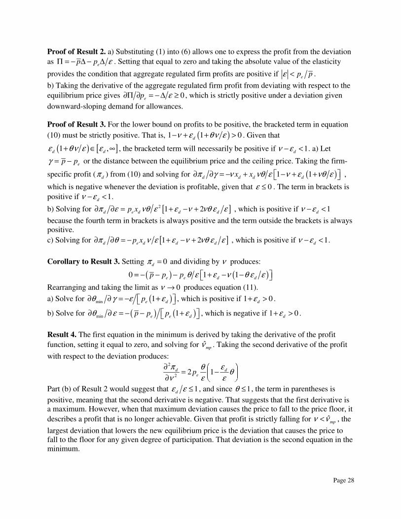
downward-sloping demand for allowances. Proof of Result 3. For the lower bound on profits to be positive, the bracketed term in equation

(10) must be strictly positive. That is, ( )1 1 0d

ν ε θν ε− + + > . Given that

( ) [ ]1 ,d d

ε θν ε ε+ ∈ ∞ , the bracketed term will necessarily be positive if 1d

ν ε− < . a) Let

ep pγ = − or the distance between the equilibrium price and the ceiling price. Taking the firm-

specific profit (d

π ) from (10) and solving for ( )1 1d d d d

x xπ γ ν νθ ε ν ε νθ ε∂ ∂ = − + − + + ,

which is negative whenever the deviation is profitable, given that 0ε ≤ . The term in brackets is

positive if 1d

ν ε− < .

b) Solving for [ ]2 1 2d e d d d

p xπ ε νθ ε ε ν νθ ε ε∂ ∂ = + − + , which is positive if 1d

ν ε− <

because the fourth term in brackets is always positive and the term outside the brackets is always positive.

c) Solving for [ ]1 2d e d d d

p xπ θ ν ε ε ν νθ ε ε∂ ∂ = − + − + , which is positive if 1d

ν ε− < .

Corollary to Result 3. Setting 0d

π = and dividing by ν produces:

( ) ( )0 1 1e e d d

p p p θ ε ε ν θ ε ε= − − − + − −

Rearranging and taking the limit as 0ν → produces equation (11).

a) Solve for ( )min 1e d

pθ γ ε ε∂ ∂ = − + , which is positive if 1 0d

ε+ > .

b) Solve for ( ) ( )min 1e e d

p p pθ ε ε∂ ∂ = − − + , which is negative if 1 0d

ε+ > .

Result 4. The first equation in the minimum is derived by taking the derivative of the profit

function, setting it equal to zero, and solving for ˆmp

ν . Taking the second derivative of the profit

with respect to the deviation produces:

2

22 1d d

ep

π εθθ

ν ε ε

∂ ⎛ ⎞= −⎜ ⎟

∂ ⎝ ⎠

Part (b) of Result 2 would suggest that 1d

ε ε ≤ , and since 1θ ≤ , the term in parentheses is

positive, meaning that the second derivative is negative. That suggests that the first derivative is a maximum. However, when that maximum deviation causes the price to fall to the price floor, it

describes a profit that is no longer achievable. Given that profit is strictly falling for ˆmp

ν ν< , the

largest deviation that lowers the new equilibrium price is the deviation that causes the price to fall to the floor for any given degree of participation. That deviation is the second equation in the minimum.

Figure 1. Analysis of the profitability of emissions allowance price manipulation

Price ($)

Abatement

Demand for Emission-IntensiveGoods and Services Marginal

AbatementCosts

ep

pΔ

A B

C D E F

1z 2z 3z 4z

p

5z

The profitability of deviating from the equilibrium allowance price is estimated by comparing

the increased cost of the deviation, depicted by the shaded region and F, with the decreased cost

of compliance from the lower equilibrium price, defined by regions A and B.

Figure 2. Profitability of deviation as a function of deviating coalition size and size of the

deviation

0% 10% 20% 30% 40% 50% 60% 70% 80% 90% 100% 0%

10%

20%

30%

40%

50%

60%

70%

80%

90%

100%

Siz

e o

f devia

tion (

% o

f tr

uth

ful dem

and)

% of emissions in coalition

Unprofitable, but new price

is constrained by floor

Profitable, but new price

is constrained by floor

Profitable

Un

pro

fita

ble

Maximum Profit Line

( )θ

(ν)

1

3

2

4

Note: The gray area is the profitable deviation triangle.

Figure 3. Profitability of deviation for various equilibrium prices and a $30 price ceiling

0% 20% 40% 60% 80% 100% 0%

10%

20%

30%

40%

50%

60%

70%

80%

90%

100%

Siz

e o

f devia

tion (

% o

f tr

uth

ful dem

and)


0% 20% 40% 60% 80% 100% 0%

50%

100%

Max P

rofit

As %

of

Tru

thfu

l E

xpenditure


Profit Triangle (pe=$15)

0.12

0.10

$30

$10

d

p

p

ε

ε

= −

= −

=

=

Profit (pe=$24)

Profit (pe=$15)

Profit Triangle (pe=$24)

(ν)

( )θ

( )θ

Note: Profit is the lower bound on theoretical profit.

Figure 4. Profitability of deviation for various economy-wide elasticities

0% 20% 40% 60% 80% 100% 0%

10%

20%

30%

40%

50%

60%

70%

80%

90%

100%

Siz

e o

f devia

tion (

% o

f tr

uth

ful dem

and)


0% 20% 40% 60% 80% 100% 0%

50%

100%

Max P

rofit

As %

of

Tru

thfu

l E

xpenditure


0.10

$30

$24

$10

d

p

p

p

ε = −

=

=

=

( )Profit Triangle 0.3ε = −

( )profit 0.3ε = −

( )profit 0.06ε = −( )profit 0.15ε = −



(ν)

( )θ

( )θ


Figure 5. Profitability of deviation as a percentage of truthful expenditure

0% 10% 20% 30% 40% 50% 60% 70% 80% 90% 100% 0%

10%

20%

30%

40%

50%

60%

70%

80%

90%

100%

Pro

fit

As %

of

Tru

thfu

l E

xpenditure


1%ν =

7%ν =

20%ν =

0.12

0.10

$30

$24

$10

d

p

p

p

ε

ε

= −

= −

=

=

=

( )θ


Figure 6. Minimum coalition size necessary to earn a 3 percent reduction from truthful

expenditure for varying deviation sizes

0% 10% 20% 30% 40% 50% 60% 70% 0%

5%

10%

15%

20%

25%

30%

35%

40%

45%

50%

Coalit

ion s

ize f

or

3%

reduction o

f tr

uth

ful expenditure

Distance between ceiling and equilibrium price (as % of ceiling)

1%ν =

0.12

0.10

$30

$10

d

p

p

ε

ε

= −

= −

=

=

10%ν =

(θ )

Flo

or-

Ind

uce

d L

imit

20%ν =

5%ν =


Table 1. Allowances issued under various planning horizons and reserve size necessary to support a

3 percent deviation

Planning

Horizon

(PH) (yrs

from 1st yr)

No. Allowances

Issued Over PH

(million)

# Allowances

Required for 3%

Deviation Over PH

(millions)

Reserve Necessary

to Support

Deviation (as % of

Year 1 Allowances)

3 15,000 450 9%

5 25,000 750 15%

10 50,000 1,500 30%

Note: assumes five billion allowances are issued in the first year.

Table 2. Upper and lower bounds on theoretical profit for various planning horizons and deviation

and coalition size settings

Planning

Horizon

(PH) (yrs

from 1st

yr)

No.

Allowances

Issued Over

PH (millions)

Coalition

(%)

Deviation (as

% of

Coalition

Demand

over PH)

Deviation

(as % of

Coalition

Demand in

1st Yr)

New Supply

(as % of total

1st Yr

Allowances)

Cost With

No

Deviation

($ million)

Cost of

Deviation

Investment

($ million)

Cost Under

Deviation

(excl. dev.

allowances)

($ million)

Minimum

Profit (eq. 10)

($ million)

Annualized

Effective Real

Return on

Deviation

Investment

from Min

Profit

Maximum

Profit

(Result 1)

($ million)

Annualized

Effective Real

Return on

Deviation

Investment from

Max Profit

5 10 30 1.5 $18,000 $450 $17,397 $153 11% $227 16%

10 10 30 3 $36,000 $900 $33,575 $1,525 41% $1,813 46%

5 10 50 2.5 $30,000 $750 $28,995 $255 7% $378 10%

10 10 50 5 $60,000 $1,500 $55,958 $2,542 23% $3,021 26%

5 10 100 5 $60,000 $1,500 $57,990 $510 4% $755 6%

10 10 100 10 $120,000 $3,000 $111,917 $5,083 12% $6,042 13%

15,000

25,000

50,000

3

5

10

Note: assumes $24 predeviation equilibrium price; economy-wide elasticity= -0.12 for all planning horizons; coalition sector-wide elasticity = -0.10 for all planning horizons; Annualized effective real return assumes deviation investment made at the beginning of the first year with profits earned each year over the duration of the planning horizon and reinvested with a 3 percent real risk free discount rate. Investing profits in a higher returning investment vehicle would increase the effective real return earned from the deviation.

1 See Harrison Fell, Dallas Burtraw, Richard Morgenstern, Karen Palmer, and Louis Preonas, “Soft and Hard Price

Collars in a Cap-and-Trade System: A Comparative Analysis,” Resources for the Future Discussion Paper 10-27

(May 2010); Terry Dinan, “Reducing Greenhouse Gas Emissions with a Tax or a Cap: Implications for Efficiency

and Cost-Effectiveness,” National Tax Journal 62(3): 535-53 (September 2009). 2 See Cedric Philibert, “Assessing the Value of Price Caps and Floors,” Climate Policy 9: 612-633 (2009); Harrison

Fell, Dallas Burtraw, Richard Morgenstern, and Karen Palmer, “Climate Policy Design with Correlated

Uncertainties in Offset Supply and Abatement Cost,” Resources for the Future Discussion Paper 10-01 (January

2010). 3 See Stephen Craig Pirrong, “Manipulation of the Commodity Futures Market Delivery Process,” Journal of

Business 66(3): 335-369 (1993); Robert Hahn and Roger Noll, “Designing a Market for Tradable Emission

Permits,” in Reform of Environmental Regulation, ed. Wesley Magat (Ballinger, June 1983); Robert Hahn, “Market

Power and Transferable Property Rights,” Quarterly Journal of Economics 99(4): 753-765 (1984). 4 See Hans H. Helbling and James E. Turley, “Oil Price Controls: A Counterproductive Effort,” Federal Reserve

Bank of St. Louis (November 1975). 5 See Lee S. Friedman, “The Long and the Short of It: California’s Electricity Crisis,” International Journal of

Public Policy 4(1/2): 4–31 (2009). 6 See Congressional Budget Office, “Causes and Lessons of the California Electricity Crisis” (September 2001). 7 See Paul Krugman, “Target Zones and Exchange Rate Dynamics,” Quarterly Journal of Economics 61(3): 669-82

(August 1991); Shawkat Hammoudeh and Vibhas Madan, “Expectations, Target Zones, and Oil Price Dynamics,”

Journal of Policy Modeling 17(6): 597-613 (January 1995). 8 See Jose M. Carrera, “Speculative Attacks to Currency Target Zones: A Market Microstructure Approach,”

Journal of Empirical Finance 6: 555-582 (1999); Christophe Chamley, “Dynamic Speculative Attacks,” American

Economic Review 93(3): 603-621 (June 2003); Stephen Salant. “The Vulnerability of Price Stabilization Schemes to

Speculative Attack,” Journal of Political Economy 91(1): 1-38 (1983). 9 Similar experiences occurred with the Mexican peso (Dec. 22, 1994), the Thai baht (July 2, 1997), and the

Malaysian ringgit (July 14, 1997). 10 See Ronald Anderson and Christopher Gilbert, “Commodity Agreements and Commodity Markets: Lessons from

Tin,” Economic Journal 98: 1-15 (March 1988). 11 See Mark Isaac and Charles Plott, “Price Controls and the Behavior of Auction Markets: An Experimental

Examination,” American Economic Review 71(3): (June 1981); Vernon Smith and Arlington Williams, “On

Nonbinding Price Controls in a Competitive Market,” American Economic Review 71(3): 467-74 (June 1981). 12 See Christopher Knittel and Victor Stango, “Price Ceilings as Focal Points for Tacit Collusion: Evidence from

Credit Cards,” American Economic Review 93(5): 1703-1729 (December 2003). 13 See Stephen Salant and Dale Henderson, “Market Anticipation of Government Policies and the Price of Gold,”

Journal of Political Economy 86(4): 627-648 (1978). 14 See U.S. EIA, “Annual Energy Outlook 2010.” Report DOE/EIA-0383 (May 11, 2010). 15 For example, allowance prices might rise dramatically if a U.S. government representative were to announce that

new nuclear energy production was unlikely, or if new information were revealed suggesting that carbon capture and

sequestration was infeasible. 16 Firms that might want higher allowance prices could include those firms that 1) are allocated more allowances

than they need and can profit from the sale of excess allowances; 2) are allocated a large share of what they need

and can make windfall profits by passing the allowance costs on to consumers; 3) hold a large bank of allowances;

4) have many opportunities to reduce their emissions at a marginal cost lower than the market price; or 5) produce a

product equivalent to the marginal priced product but that requires fewer (or no) allowances in its production than

the marginal product. An example of the last case would be a nuclear plant that produces electricity using no

allowances but would benefit from high allowance prices in setting its electricity rates when coal or natural gas are

at the margin. For a discussion of the first two examples, see James B. Bushnell, Howard Chong, and Erin T.

Mansur, “Profiting from Regulation: An Event Study of the EU Carbon Market,” National Bureau of Economic

Research Working Paper 15572 (December 2009). 17 Those public good benefits and the incentive to free ride are also present in the decision whether to adopt

abatement technologies. See Till Requate and Wolfram Unold, “Environmental Policy Incentives to Adopt

Advanced Abatement Technology: Will the True Ranking Please Stand Up?” European Economic Review 47: 125-

146 (2003); Jinhua Zhao, “Irreversible Abatement Investment under Cost Uncertainties: Tradable Emission Permits

and Emissions Charges,” Journal of Public Economics 87: 2765-2789 (2003). 18 For an example of tacit cooperation strategies in auctions, see Peter Cramton and Jesse A. Schwartz, “Collusive

Bidding: Lessons from the FCC Spectrum Auctions,” Journal of Regulatory Economics 17: 229-252 (May 2000). 19 That is, firms can bank allowances from one compliance period to the next within period T or borrow allowances

from a future compliance period within period T , assuming that period T , or the planning horizon of the economy,

is more than one compliance period long. 20 The upper bound on profit, as derived in Appendix A, can also be calculated using just the elasticity of demand

for allowances. 21 See Mark Lasky, “The Economic Costs of Reducing Emissions of Greenhouse Gases: A Survey of Economic

Models,” CBO Technical Paper (May 2003). The models analyzed for the CBO model include the EIA’s National

Energy Modeling System (NEMS), the Emissions Prediction and Policy Analysis (EPPA) model used by climate

researchers at the Massachusetts Institute of Technology, the Applied Dynamic Analysis of the Global Economy

(ADAGE) model developed at RTI International and used by EPA, the Second Generation Model (SGM) and

MiniCAM models developed and used by the Joint Global Change Research Institute, the Model for Evaluating the

Regional and Global Effects of GHG Reduction Policies (MERGE) developed by Stanford University and the

Electric Power Research Institute, and the Multi-region National-North American Electricity and Environment

(MRN-NEEM) model developed and used by CRA International. 22 See also Congressional Budget Office, How CBO Estimates the Costs of Reducing Greenhouse-Gas Emissions, Background Paper (April 2009). 23 Those elasticities ( ε ) of allowance demand to changes in allowance price are a transformation of economy-wide

elasticities published earlier by CBO as referenced in footnote 21. Specifically,

( ) ( ) ( )2 1 1 1 21B A B A A A A

P P P P P P Pε

ε ⎡ ⎤= − − − −⎡ ⎤⎣ ⎦⎣ ⎦

% , where ε% is the previously published economy-wide elasticity of

emissions to changes in the base price (B

P ) of carbon. 1AP and 2A

P are two allowance prices around which the

elasticity of allowance demand is defined. 24 For emissions shares, see U.S. EIA, “Annual Energy Outlook 2010.” Sector-specific elasticities were derived

using a methodology similar to that used to derive CBO’s economy-wide elasticity, using data and elasticity

estimates from the models listed in footnote 21. 25 Data compiled by Point Carbon, “Carbon Exposure: Winners and Losers in a U.S. Carbon Market” (November 2,

2009) from the Carbon Disclosure Project, EIA, and Christopher Van Attan, Thomas Curry, and Amlan Saha,

“Benchmarking Air Emissions of the 100 Largest Electric Power Producers in the United States” (May 2008),

funded by CERES, the Natural Resources Defense Council, PG&E Corporation, and the Public Service Enterprise

Group. 26 A 10 percent deviation with a 5 percent coalition over a 5- year planning horizon would require deviating firms to

increase the overall supply in the first year by 2.5 percent while increasing the number of allowances they would

have purchased in the first year by 50 percent. 27 See Robert Stavins, “A Meaningful US Cap-and-Trade System to Address Climate Change” Harvard

Environmental Law Review 32(2): 293-372 (2008) who suggests that a ceiling set 2 to 10 times above the expected

allowance price level would bind only in the most volatile situations.

unintended consequences of price controls: an application

Documents