JOURNAL OF DIFFERENTIAL EQUATIONS 45, 207-233 (1982)

Uniform Bounds from Bounded.&-Functionals in Reaction-Diffusion Equations

F. ROTHE

Lehrstuhlj Biomathematik, Universitcft TCbingen, Auf der Morgenstelle 28, 7400 TCbingen, West Germany

Received April 8, 198 1; revised August 10, 198 1

To prove global existence of classical or mild solutions of reaction-diffusion equations, a priori bounds in the uniform norm are needed. But for interesting examples, often one can only derive bounds for some L,-norms. Using the structure of the reaction term they can be used to obtain uniform bounds. Two propositions are stated which give conditions for this procedure. The proofs use the smoothing properties of analytic semigroups and the multiplicative GagliardeNirenberg inequality. To illustrate the method, we prove global existence of solutions for the Brusselator and a Volterra-Lotka system with one diffusing and one sedentary species.

INTRODUCTION

Reactiondiffusion equations have been studied in recent years in different contexts. Due to the structure of the reaction part a vast variety of interesting phenomena can occur, which are hard to study by analytical tools. Even the relatively simple problem of proving existence of solutions globally in time and the intimately related problem of obtaining a priori bounds are nontrivial.

Concerning these questions, the situation is very similar for the initial- value problem of ordinary differential equations and the initial-boundary- value problem of semilinear parabolic equations.

In both cases, the solution may “explode” after a finite time T (see also Ball [6]). To exclude this phenomenon for semilinear parabolic equations, one needs a priori bounds.

Semilinear parabolic equations can be studied in different functional spaces. The well-known Holder spaces lead to classical solutions (see Friedman [8] or, in a more functional analytic representation, Kielhiifer [ 121 and Henry [lo]). Nevertheless, it turns out that estimates in the uniform norm do as well and that the considerations can be generalized to mild solutions in the space of bounded measurable functions.

207 0022-0396/82/080207-27$02.00/O Copyright 0 1982 by Academic Press, inc.

All rights of reproduction in any form reserved.

brought to you by COREView metadata, citation and similar papers at core.ac.uk

provided by Elsevier - Publisher Connector

208 F. ROTHE

Thus it is our aim to obtain a priori bounds in the uniform norm. Note that due to the destabilization effect of diffusion (Turing [ 211) the

solution of the reaction-diffusion system may be unbounded, even if the solutions of the corresponding reaction system are bounded. Thus one has to study the whole reaction-diffusion system.

For many reaction-diffusion systems studied in applications like the Volterra-Lotka system, the Brusselator (Prigogine and Glansdorff [ 17]), the Gierer-Meinhardt morphogenesis model [ 161, and the Keller-Segel chemotaxis model (see, e.g., Rascle [ 181) it is intuitively clear that the solutions remain bounded globally in space and time. But there is no general method to prove such a result for a wide class of equations.

The well-known method of invariant regions (which is in principle a multidimensional version of the maximum principle; see, e.g., Chueh et al. [?I) fails for the quoted examples.

In the following we construct uniform bounds for a restricted class of problems. Our approach is inspired by the work of Alikakos on the Volterra-Lotka system [3] and porous media equations [4].

We proceed in two steps. In the first step we construct a functional of the solution which can be bounded a priori. For this step, similar to the situation in Ljapunov functionals, we do not have a general method. As examples we treat the Volterra-Lotka system and the Brusselator. In the second step, we prove that a priori bounds for the functional constructed above imply uniform a priori bounds. To this end one arranges the equations in a convenient order and constructs bounds for u,, u?,..., u, successively. To get a uniform bound for one component, e.g., U, , the following information (obtained in step (1)) will be used:

(1) The dependence of the reaction term in the equation for U, on U, and the other components (which are considered as “weight functions”).

(2) ,$-bounds for the component U, . (3) L,-bounds for the weight function involving the other components.

Propositions 1 and 2 give detailed conditions under which assumptions (l), (2), (3) are strong enough to derive uniform bounds.

In many cases of ecological models a natural order of the variables u1 ,***, u, is given by the food pyramid condition (see, e.g., Williams and Chow [23]). It seems natural to use this order in our context as is done by Alikakos in [3].

Some cases in Example 1, a Volterra-Lotka system with sedentary prey and diffusing predator show that this may not be possible. Nevertheless, this example can be dealt with by exploiting the weight function introduced in Propositions 1 and 2. Thus we cover a wider class of problems than was examined in [3].

BOUNDEDL,-FUNCTI~NALS 209

The paper is organized as follows: In the first section we give basic notation and definitions as well as the existence and uniqueness theorem for semilinear parabolic equations in a mild and a strong version: Here the “maximal existence time” is introduced and the usefulness of a priori bounds becomes clear.

The second and third sections state and prove two propositions, achieving the second step in the construction of a priori bounds explained above. Proposition 1 is proved by an iterative procedure of estimates for )I u]]~,.~, v = 0, l,..., where in each step the multiplicative Gagliardo-Nirenberg inequality is needed. Proposition 2 is weaker in the case of dimension n = 1, but allows a much more lucid proof using analytic semigroups. Here the multiplicative estimate appears only in the elementary form I] u& <

Il~ll~-r’p I141:‘p and the iteration procedure is avoided by a “feedback” argument reminiscent of summing up a geometric series. Nevertheless we give the two proofs, because they possibly allow generalizations in different directions.

The fourth section contains two examples, a Volterra-Lotka system and the Brusselator, for which the whole construction of a priori bounds is done.

It remains to relate this article to the work of Kielhofer [ 131 and von Wahl [22], who both prove global existence for semilinear parabolic equations.

Kielhofer’s first step is to obtain an energy inequality. This can be done for the Navier-Stokes equations but is not possible for reaction-diffusion equations unless the reaction term is linearly bounded.

Both Kielhiifer and von Wahl consider only Dirichlet boundary conditions and restrict the growth-rate of the nonlinear term (denoted by y) more severely than we do. They do not get global bounds independent of time (which are needed to get compactness of the trajectories used in the study of asymptotic behavior) as in this article. Hopefully the results and ideas of this article can be applied to a quite large class of reaction-diffusion equations. It remains an open problem to characterize this class in detail.

After this paper was completed we became aware of the work of Massatt [24]. Massatt proves a result similar to Proposition 2 under the additional restrictions r > y and q = a~ (no weight function).

In that case one has an L,-bound of the right-hand side F(x, t, u). Using the bootstrap argument as in Proposition 2 (without the multiplicative splitting of the right-hand side and the “feedback” argument) one gets in a finite sequence L,, , L, *,..., L, estimates for u.

The condition r > (y - 1) n/2 is necessary for this to work. The advantage of our feedback argument is that we do not need the additional assumption r > y and that we get a simple explicit formula for the L,-bound.

210 F.ROTHE

1. LOCAL EXISTENCE OF SOLUTIONS

Some definitions are needed. Let R c R” be a bounded domain with boundary of class C *‘” for some v E (0, 1). The usual norms in the spaces L,(Q), L,(0) and C(fi) are denoted by

Note that the norm ](u](, is increasing in p, since the factor l/IQ] has been introduced.

In the following, the operator -A + 1 is denoted by A, where different function spaces are used and Dirichlet or Neumann boundary conditions occur according to the boundary conditions in the main initial-boundary value problem (5), (6), (7) considered.

More exactly, by A” we denote the operator given by

D(J)= I uEC2@)]~=OonaR ,

I

,&=(-A+ 1)~ for 24 E D(J).

It is well known that the operator A’ is closable in the Banach spaces L, for p E (1, co). The closure A, generates an analytic semigroup Tp(t) = emApf. Another definition of 7”(f) using interpolation is given by Reed and Simon [ 19, TheoremX.55, p. 2551. The corresponding operators can be defined for Dirichlet boundary conditions. In this case Kielhiifer [ 121 constructs also a semigroup T,(t) in the space C”(a). Because of an additional singularity at f = 0 this is not a strongly continuous semigroup, but many properties of analytic semigroups can be retained. Let L be the smallest positive eigenvalue of A,u = Au. (Hence I = 1 for Neumann boundary conditions.)

LEMMA 1. (1) The semigroups T,(t), T,(t) are positivity preserving; i.e.,

u(x) > 0 forallxEd

implies

(T(t) u)(x) a 0 forallxE6, t > 0.

BouNDED L,-FUNC~~NALS 211

(2) For any p, q such that 1 < p < q Q 00 and any 6 > 0 there exists a constant K,(n,p, q, 6,&S) such that

11 T,(t) uJlq < K,(l + t-“‘2(“p-“q)-6) e-‘3’ (Ju(Jp. (1)

For n = 1 or heat equations with Dirichlet boundary conditions, one may choose 6 = 0.

(3) For any v E (0,2) and any 6 > 0 there exists a constant K,(n, v, 6, f2) such that

IIT,(t)ulJ,,<K,(l + t-‘“‘2+6))e-atIJul(,. (2)

Remark. All statements above remain valid if -d is replaced by any uniformy elliptic operator of second order.

Prooj (1) This is the weak maximum principle. (2) The constants K depend on the exponents involved and on a. Let

p E (1, a~), a E (0, 1). By analytic semigroup theory (see Henry [IO])

ll~;~p@)4lpGGt-” IblIp and by embedding theorems

Ibll,UG ll~;~ll, for

Hence one gets

4 E [L al, l/q > l/p - 2a/n.

(I Tp(t) ull, < K5t--ln’2(“p--‘q)+S1 I(uJ(, * (3)

for 1 <p < q Q co, 6 > 0 and n/2 (l/p - l/q) < 1.

The last restriction is removed by using the semigroup property and iteration.

Note that the case q = co is included. Using (T(t) p, w) = (o, T(t) w) for all p, w E L,(Q), the case p = 1 can

also be included by a duality argument. Hence (3) is valid for 1 Qp Q q < 00, 6 > 0.

By elementary Hilbert space arguments

II T2W 41z G e-*’ l1412. (4) Now the result follows by putting (3) and (4) together and using the semigroup property.

212 F. ROTHE

Take the case of Dirichlet boundary condition. We define

4% 0) = I u,(x)1 7 x E J-2,

= 0, xER”-R,

and let U(X, t) satisfy the heat equation vI = A for x E R”, t > 0. Then

v(x, t) = R” (47ct)-“/* exp - (x ~~‘)* i 4% 0) &

and an explicit calculation shows

for 1 <p<q< 00. By comparison arguments we have

(u(x, t)l Q v(x, t) e-l’

and hence (1) is valid with 6 = 0. (3) ForV<2a-n/pwehaveIlull,,<KIIA;ullP(see [lo]).

For the convenience of the reader, we state the existence and uniqueness theorem for systems of weakly coupled reaction-diffusion equations in a mild and a classical form.

Let x = (x1 ,..., x,) E R” and u = (u, ,..., u,) E R”. D = diag(d, ,..., d,) denotes the nonnegative diagonal matrix of the diffusion coefficients. (di > 0 may be zero.) The function

models the reaction terms and the function u,,: fin-1 R” gives the initial data. Considering mild and classical solutions, respectively, we need assumption

(M) or (S) for f and u,.

(M) Let f be measurable with respect to (x, t, u). For (x, t, u) and (x, t, u) in any bounded set B c 0 X [0, co) X Rm let f be bounded and satisfy

If(x, 6 ~1 -f (xv f, VII < L(B) I u - v I.

Let u,, be measurable and bounded on d (S) Let (M) hold. On any bounded set BcD x [0, co) x R” letfbc

uniformly Holder-continuous. Let u0 be uniformly Holder-continuous on 0.

BOUNDED L,-FuNCTI~NALE~ 213

Take a weakly coupled system of reactiondiffusion equations

au/at - DAu =f (x, t, u) forxER, t>O (5)

with initial conditions

4% t) = u&) forxE0 (6)

and boundary conditions of Dirichlet

u(x, t) = 0 forxE80, t>O 0)

or Neumann type

g (x, t) = 0 for x E XI, t > 0. (7b)

Also the case of different boundary conditions for different components can be included.

Let the semigroup T(t) of operators Z,,(n)“’ -+L,(a)m be defined by the solution of the pure diffusion equation

u,-DAu+Du=O

with same boundary conditions as above. The operators T(t) satisfy (] T(t)/1 < 1 but do not define a strongly continuous semigroup. Nevertheless they are useful to construct mild solutions.

Clearly the operator T(t) acts componentwise and we have T(t) = (T”‘(t), T(*)(t)), where T”‘(t) = T,(d,, t)lr,cm; especially Tfu’(t) = E if d,, = 0.

DEFINITION. A mild solution of initial-boundary value problem (5), (6), (7) is a measurable function u: (x, t) E fi x [0, T> + Rm such that u(-, t) E L,(Q) and

u(., t) = T(t) u. + i,; T(t - r)f’(., 7, u(-, 7)) dt

for all t E [0, T],

where f(x, t, u) =f(x, t, u) + Du.

The following theorem is nearly standard.

(8)

THEOREM 1. Assume (M) holds.

(1) For each initial function u,, E L,(fi)m there exists T > 0 such that the initial boundary value problem (5), (6), (7) has a mild solution on [0, T).

214 F. ROTHE

(2) The “existence time T’” can be chosen maximal; in that case either T=coor

(3) Consider the existence time T as ‘a functional of the initial data uO. Then inf{T(u,) ~~~~~~~~ GM} > 0 for all M.

ProoJ Parts (1) and (3) are proved by the standard Picard-Lindelof iteration.

It remains to show (2): Assume the maximal existence time T is finite. First we show that the assumption

sup Ilwll, < c < 00 O<t<T

(10)

leads to a contradiction. For simplicity the spatial arguments x is omitted. Choose v E (0,2) arbitrary. By writing out integral equation (8) in components and applying Lemma l(c) to the components with diffusion, one gets

suP II”i(tIICu < O” if di + 0 S<t<T

for any 6 > 0. Using again the theory of analytic semigroups we get by similar

argumentsfora,C1E(O,l),pE(l,ao)suchthata+y<l,v<2a-n/p

if di # 0. (11)

Introduce the norm

II~lln=II~Ilm+ 2 d~ll~ill~u~Il~ll~+~ 2 diIIAp”Uillp- i=l i=l

We have shown

sup II Wlln GM < co. S(t<T

Next we show that

$ u(t) exists in the norm II II,, . (12)

Let the sequence t, be increasing and lim,,, t, = T. Let t, > tn.

215

It is easy to see that the integral equation (8) implies

an) - GJ = vvm - GJ -El at)

I h--In + T(‘)(t,,, - t, - t)j& + r, u(t, + 5)) ds. (13)

0

We distinguish the components with di = 0 or di # 0. If di = 0, (13) implies

II Gn> - at)ll,

If di # 0 we have

+ 0

.tm--l” [IA; ~‘i)(r)llp,p dr) su~{ll.k ~)llco, 0 < 5 < T II ~11, < (3. 0

Since by analytic semigroup theory (IA;” - E)]] < C’t”, since (11) holds and since the integral using ]]A,” T”‘(r)]] <Kc*, can be estimated we have ]] u(t,) - u(t,)]], --f 0. Now since lim,,, u(t) exists, the mild solution can be prolonged to an interval [0, T + E), which contradicts the maximality of T. This shows that (10) cannot hold and hence

(14)

We assume

lim $f ]] u(t)]], < r < co (15)

and derive a contradiction. If (14) and (15) hold, there exist sequences (t,) and (t,,J such that

tm<r,,limt,=limr,=Tand

II 44nIlm = I,

II ~(5n>llco = r + 1,

II Wlla, G r + 1 for t E [tm, r,]. From the integral equation

u(r,) = T(r,,, - cm) u(t,) + i,;m-tm T(t, - t, - o)f(u(t, + a)) da

216

one gets

F.ROTHE

hence r + 1 < r, which is a contradiction. Thus (15) cannot hold and we get

which proves (2). The arguments of this proof are similar to those of Henry [lo] and Ball [6].

Clearly one can also prove (2) using (3) and repeated continuation of the solution: Suppose T,,,,, < 03 and let (9) be violated. Then there exists an increasing sequence t, converging to T,,,,, such that I] ~(t,,)]]~ < M. By (3) there exists S > 0 and mild solutions on [t,, t, + 6) with initial data u(t,). Hence by uniqueness there exists a mild solution on [0, T,,,,, + S) which contradicts the maximality of T,,,,,.

The classical existence result is

THEOREM 2. Assume (S) holds.

(1) For each initial function u,, E C”@)“’ (V E (0,2) arbitrary) the initial-boundary value problem has a unique solution for t E [0, T).

Parts (2), (3) are valid as in Theorem 1.

ProoJ: We begin with the mild solution constructed in Theorem 1. For the component with diffusion di # 0 we proved in Theorem 1

ui E c((o> T)9 c”(fi))*

For the components without diffusion (di = 0) by elementary arguments about ordinary differential equations one gets again ui E C([O, 7’), C’(a)). Hence the result follows from the interior Schauder estimates (see Friedman

PI). Remark. Theorem 2 is a special case of many well-known results (see,

e.g., Kielhtifer [ 121 and Henry [lo]). The only new point is the better characterization (9) of the maximal existence time, which envolves only the L,(Q)-norm.

BOUNDED L,-FuNCTI~NAL~ 217

2. ITERATIVE METHOD TO GET UNIFORM A PRIORI BOUNDS

If u is one component of a weakly coupled reaction-diffusion system and T is less than the maximal existence time (for simplicity take d = I), we get the following situation: Let the functions

u:(x,r)Efix [O,T] -+R,

f: (x, t, u) E d x [0, T] x R + R,

u,:xEfi +R

be bounded and measurable. We assume either

(Sl) The functions u,, , u, f are continuous and the derivatives u,, Au are continuous on Q x (0, 1”) and they solve the initial-boundary value problem

u,--Au=f for (x, t) E Q X (0, T), (16)

4x, 0) = uo(x) forxEQ (17)

with either a Dirichlet

24(x, t) = 0 for (x, t) E 80 X (0, 7) W-W

or a Neumann boundary condition

g (x, t) = 0 for (x, t) E 80 X (0, T), (18b)

or more generally,

(Ml) no additional regularity and

u(-, t) = T(t) u. + I,’ T(t - t)&, t, u(., t)) dt for all t E [0, T], (19)

here T(t) denotes the semigroup Tp(f)ILmtRb, andT(x, t, u) =f(x, t, U) + u. In the second case, we say u is a mild solution of the initial-boundary

value problem (16), (17), (18). For the reaction term we need some growth estimate. Let c: (x, t) E

d x [0, T] -+ R + be a measurable function. We assume either the one-sided estimate

U>O and f < c(1 + u)’ (20)

505/45/2 6

218 F.ROTHE

or a two-sided estimate

Ifl G 41 + IUD’.

The case T = 03 can be included.

(21)

PROPOSITION 1. Let u be a mild or strong solution of the initial- boundary value problem (16), (17), (18) and let the reaction term satisfy either the one-sided or the two-sided growth condition (20) or (21), respec- tively.

Let

u, := II 4.3 O)llco,

C := max(L ozyT 114., t)ll,),

U, := max(L Uo, owT II u(-, OllJ

y < 1 + r(2/n - l/q) (22)

then there exists a constant K(n, y, q, r, J2) and o, p(n, Y, q9 y) independent Of T such that

SUP II 4.9 t)ll, < KC‘V. o<t<r (23)

Here one may choose

(Y- l)(l + 2/n) ’ = exp r(2/n - l/q) - (y - 1)’

1 + 2/n (y- 1X1 + 2/n) ‘=r(2/n- l/q)-(y- l)exp2r(2/n- l/q)-((y- 1)’

The proof will proceed in several steps. In the first step we get from U, an estimate of Uzr:

LEMMA 2. Under the assumptions of Proposition 1 there exists a constant K,(n, y, q, r, 0) independent of T and decreasing in r such that

U,, < K,(n, y, q, r, f2)‘lr (2rC)““’ Uf(“, (24)

where

u(r) = l/2 + l/n

G/n - l/q) - (Y - 1)

BOUNDEDL,-FUNCTIONALS 219

and

p(r) = @/n - l/d + (y - 1)(1/n - l/2) = 1 + (y _ 1) o(r)

Wn - l/q) - (Y - 1)

Proof of the lemma. For definiteness, the case of Neumann boundary conditions, one-sided estimates and classical solutions is considered: Multiplying the differential equation (16) on both sides by uzr-’ yields, after a partial integration,

d 1 -- i dt2r D

uzr dx + v (, (VZ/)~ dx

= I fu 2r--l a!x < c(l + u)Yd-’ dx. n I R

After introduction of w = u’ as new variable one gets

dl 1 --- dt 2r lii?( I

2r-1 1 R w2dx+-- 1 r2 Ial D

w2ak+, /(l +w2”)dx. (25) I

For the meaning of a see (29) below. The inequality (a + b)’ < 2”(aP + bP) for p > 0; a, b > 0 has been used. The following three steps (26) through (28) are essential. Denote the left-

hand side of (25) by L. All norms are taken with respect to the spatial variable x whereas time occurs as a parameter.

L G 2y~ll~ll, + ll4ls II 4l::J’ (26)

L G 2y~l141, + llcll, ((~3/2)Ol4ll + Ib# llwl:-4N2”l < 2y[llcll, + l141p~:“(llwll:” + lIWlI:Q4 IlwI:n(‘-8Y, (27)

L G 2y~l141, + llcll, Gaw41:a + E llw: + (e- (l-4)/2&3 11 WII,)204/(1-a(l-8)))]. (28)

In (25) and the following a is defined as

2a = (l/r)(y - 1 + 2r).

In (26) the Holder inequality was used, hence

l/q + I/q’ = 1.

In (27) the Gagliardi-Nirenberg inequality

(29)

(30)

II WIIZaq’ G K&Q, 2aq’)

2 (IIWIII + IbIll: llv41:-4) (31)

220 F. ROTHE

(see Ladyzenskaja [ 141) in the version without boundary conditions was used. Hence

1/2q’a=P+(1/2- l/n)(l-P) with /?E [0, 11. (32)

Note that K, depends on Q and the exponent 2aq’. In (28) Young’s inequality was used; hence E > 0 is arbitrary and we must have

ar(1 -p> < 1. (33)

By choosing E such that

and using PoincarC’s inequality

~,II~ll:~Il~~ll:~~~II~II:

(here K&2) is the smallest positive eigenvalue of -Au = Au, i3u/i.h = 0, hence depends only on Q) one arrives at

+ 2r-1 2r2

(:;?I’, K:” l[c~~q]l’(l-a(lal IIWll;a4/(1-a(l-4)),

By integration one gets

GXmax [

2Y+ 19

Gr9 G” + c2r- ljK, Will +G I141q Go”) 1 (

2Y+lr=

G‘$ (2r- 1) K:” Il4) l/Cl-u(l-4))

2m!3/(1-o(1-4)) u, . (34)

Before simplifying this expression, one must make some considerations concerning the exponents involved. For precribed values of the exponents n, y, q and r the values of a, q’ and /I are given by (29), (30) and (32), respec- tively. Some computation shows that condition (33) can only be satisfied if

y < 1 t r(2/n - l/q). (22)

BOUNDEDL,-FUNCTI~NALS 221

Thus assumption (22) is necessary for the proof to work. Conversely assume (22). Then by choosing

a= 1 + (y- 1)/2r, (35)

p = P/n - l/d + (l/n - VW - 1)/r (1 + 2/n)@ + (Y - 1)/V (36)

(29), (30) and (32) are satisfied. Since (1 + 2/n) a(1 -p) = (y - 1)/r + 1 + l/q, the basic assumption (22) implies (33). As an easy consequence of 0 < a( 1 - p) < 1 we have /3 E (0, 1). The important term in the cumbersome expression (34) is the last one, because there the largest powers of ((cl] and I] u )I occur. The relevant exponents are

1 l/2 + l/n 2r( 1 - a( 1 -/I)) = o(r) = r(2/n - l/q) - (y - 1)’

aP wn - l/q) + (Y - l)ul~ - l/2) 1 - a(1 -/I)

E p(r) = G/n - l/q) - (Y - 1) *

Since a > 1 and p/( 1 - a( 1 - /I)) > 1 expression (34) can be simplified to

U:; < max[ Vir, KCZro(r)U:rp(r)], (37)

l/Cl--u(l--4)) K=l+ (2r-l)K,

2y+‘r2 (1 + K;@) + & (g+) .

Using the dependence of a, p and K,(R, 2aq’) on I one see that K can be estimated by

where

K < K;(n, y, q, I, f2)(2r)2ro(r) with 1 <K,,

1 1 + 2/n 2ru(r)= l-a(l-/3)=(2/n--l/q)-((y-1)/r

and K, are decreasing functions of r. Taking the 1/2r power yields

U,, < max [ V,, K:“(2rC)““’ IV;(~)].

Since K, > 1, 2rC > 1 and p(r) > 1 this implies the desired formula (24). The whole argument can be done for mild solutions as well, if one uses the

inequalities in a time-integrated form.

222 F. ROTHE

Proof of Proposition 1. The proof of Proposition 1 now uses an iterative procedure. By induction, formula (24) implies

where

s = L+ G”r) + @“r) @“- ‘r) + ’ 2”r 2”-‘r 2u-zr *‘*

+ p(2”r) ~(2”~‘r) se. p(r) ,

r

6, = vu(2”r) + (v - 1) p(2”r) a(2”-‘r)

+ (v - 2)p(2”r)p(2”-‘r) a(2”-*r) + ..a

+ lp(2”r)p(2”-‘r) .e. u(2r),

6, = a(2”r) + p(2”r) u(2”-‘r) -t p(2”r)p(2”-‘r) a(2”-*r) + ...

+p(2”r)p(2”-‘r) .a. p(2r) u(r),

6, =p(2”r)p(2”-‘r) es. p(r).

Using the formulas u(2r) < u(r)/2, p(r) = 1 + (y - 1) u(r) we get

6, < (1 + (Y - 1) u(r))( 1 + (y - 1) u(r)/2) ..a.

Taking logarithm and summing up the geometric series yields

ln 6, < 2(y - 1) u(r),

6, < exp 2(y - 1) u(r) = exp (Y- l)(l + 2/n) @ln- V7)-(~- 1)’

Similarly

6, < [u(r) + u(2r) + u(4r) .. . ] p(2r) p(4r) ...

< 2u(r) exp 2(y - 1) u(2r)

1+2pn (Y - 1x1 + WI = r(2/n - l/q) - (y - 1) exp 2r(2/n - l/q) - (v - 1)’

s,<[l.u(2r)+2.~~(4r)+3.u(8r)...]p(2r)p(4r)~..

< 4u(2r) exp 2(y - 1) u(2r),

6, < $p(r)p(2r) . es < + exp 2(y - 1) u(r).

BOUNDED L,-FUNCTIONAL~ 223

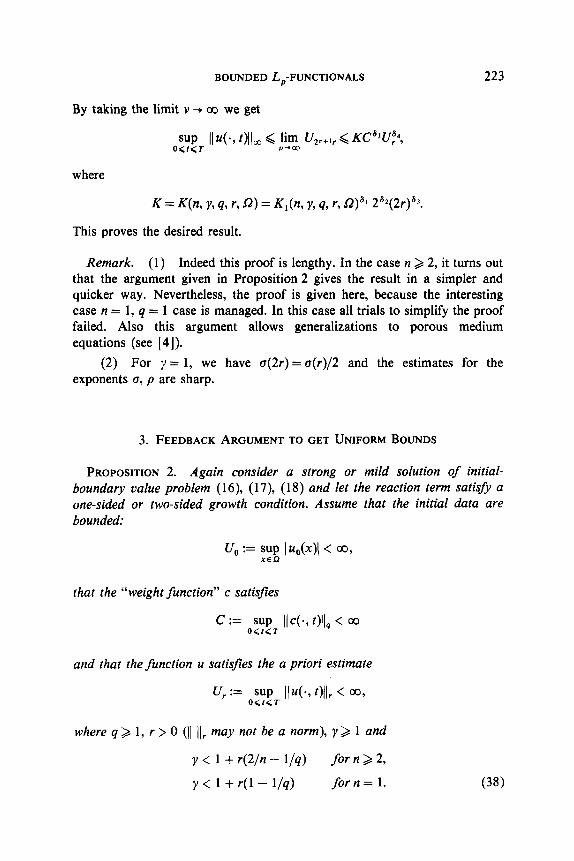
By taking the limit v + 00 we get

where

K = K(n, y, q, r, J2) = K,(n, y, 4, r, 0)“’ 2”(2r)“.

This proves the desired result.

Remark. (1) Indeed this proof is lengthy. In the case n > 2, it turns out that the argument given in Proposition 2 gives the result in a simpler and quicker way. Nevertheless, the proof is given here, because the interesting case n = 1, q = 1 case is managed. In this case all trials to simplify the proof failed. Also this argument allows generalizations to porous medium equations (see [4]).

(2) For y = 1, we have a(2r) = o(r)/2 and the estimates for the exponents u, p are sharp.

3. FEEDBACK ARGUMENT TO GET UNIFORM BOUNDS

PROPOSITION 2. Again consider a strong or mild solution of initial- boundary value problem (16), (17), (18) and let the reaction term satisfy a one-sided or two-sided growth condition. Assume that the initial data are bounded:

that the “weight function” c satisfies

c := WT IId- f)llq < CQ

and that the function u satisfies the a priori estimate

ur := $r& IIu(*, t)ll, < m,

where q > 1, r > 0 (11 III may not be a norm), y> 1 and

y < 1 + r(2/n - l/q) for n > 2,

y < 1 + r(1 - l/q) fern= 1. (38)

224 F. ROTHE

Then for u chosen as explained below, let p = 1 -t (y - 1) u. There exists K = K(n, y, r, q, o, 52) such that

sup IIu(-, t)ll, < K[(l + U,,) + (1 + C)(l + Ur)p’O]O. (39) OSf<T

Choice of u: Define

uo= [r(l- l/q)-((y- 1)]-’ fern= 1

= [r(2/n- l/q)-((y- l)]-’ forn>2.

First let n = 1. Choose u = max( 1, uo). Now let n > 2. Zfu, < 1 choose u = 1. Zf u. > 1 choose u > u. and u - u. arbitrarily small.

Proof: Clearly f”=f + u satisfies the growth condition (20) or (21) with c replaced by (1 + c).

First we consider the case of the one-sided estimate. Then by the maximum principle formula (19) implies

0 < u(., t) < U, + .’ T,(t - z)( 1 + c)( 1 -t ) ZJ 1)’ (5) dz. ! 0

From the two-sided estimate we get

lu(.,t)l~Uo+jo~T,(t--r)(l +c)(l +lul>‘(7)dz, (40)

which is valid in either case. In the following we choose

PE [Loo), P > n/2 (41)

and consider the semigroup Tp(t) as an operator from L,(G) to L,(Q). Lemma l(b) implies

Using (42) in formula (40) yields

sup O<f$T

]]u(., t)]lW < Vo +K, oz;T ]I(1 + c)(l + ]u])‘]],.

Using Holder’s inequality we arrive at

(42)

sup II 4.9 OIL < uo + K,(l + C) o.yyT II 1 + l4.v 01 IL (43) OCf<T

BOUNDEDL,-FUNCTI~NAL~ 225

where s has to satisfy

l/P = l/q + l/s, SE [l, a)]. (44)

A particularly simple situation occurs if

l/sy > l/r.

Then the left-hand side of (43) can be estimated directly. We get

(45)

sup II u(*, t)lloo < u, + K,(l + C)(l + U,)? (46) OCtCT

It turns out that condition (45) together with (44) and (41) can be satisfies if and only if

Y < @/n - l/q) for n > 2,

Y G r(l - l/q) fern= 1. (47)

Now take the case that (47) is violated; then (45) is also violated and we have r < sy. Splitting the last term in (43) yields, after some trivial com- putations,

< 1 + u, +K,(l + C) osu,pT(l + I[u(., f)lJJ-r’S (1 + UJ? (48)

Under the condition

y - r/s < 1 (49)

formula (48) contains a “feedback” and implies

sup Ilu(*, t)llm <K,[(l + U,) + (1 + C)(l + UJ’S]l’(‘+r’s-Y), (50) Oit<T

where K, = max( 1, K,). The important exponents are

1 ‘=l+r/s--y

and 4s ‘=l+r/s--y

= 1+ (y- I)a.

It remains to fulfill conditions (41), (44) and (49). Some computations show that

y < 1 + r(2/n - l/q)

y < 1 + r(1 - l/q)

for n > 2,

for n = 1 (38)

226 F.ROTHE

is necessary for our argument to work. Conversely assume (38) is satisfied. First let n = 1. Then one chooses p = 1 and gets

1 u = u” = r(1 - l/q) - (y - 1) ’ p=po= 1 +(y- l)a,.

In the case n > 2, choose p > n/2, p - n/2 arbitrarily small. One gets

1 a=r(l/p- l/q)-(y- 1)’ p=l+(y-l)o

and hence u > uo, p > po, where u - uo, p - p. are arbitrarily small and

1 u0=r(2/n- l/q)-@- 1)’ po= 1 + (y- l)u,.

Note that condition (38) is equivalent to u. ( 1 for n > 2 and u. Q 1 for n= 1.

Hence the assertion follows from formulas (46) and (50).

4. EXAMPLES

(a) Volterra-Lotka System with One Sedentary and One D@lusing Com- ponent

The densities of the two species are given by the functions u and u defined for (x, t) E fi x [0, 7). The dynamic is governed by the differential equations

u, = uPI + a,,u + a12ul, u, - Au = u[b2(u) + a2, u + a,,u]

together with initial conditions

(51)

for x E Q (52)

and Neumann boundary conditions

g (x, t) = 0 for (x, t) E a0 x (0, Z) (53)

for the diffusing component. Let the initial data uo(x), uo(x) be positive, bounded and Holder-

continuous. Following Goh ]9] we assume for the differential equations (5 1):

BOUNDEDL,-FUN~TI~NALS 227

The functions b,(.) and b,(e) are Lipschitz continuous and nonin- creasing, the matrix aik satisfies

a,, SO, a22 S 0, u12a2, + 0 and a12a2, S a11a22.

There exists a unique positive equilibrium 6 > 0, v^ > 0 such that

O=b,(u”)+u,,u^+a,,v^,

0 = b,(C) + a21 u” + u22 6. (54)

PROPOSITION 3. Under conditions C, listed in Table I, the solution of the initial-boundary value problem (51), (52), (53) exists globally in time (T = a~) and satisfies

Under conditions C, the solution satisfies even (55) and

so”f: IId- Ollco < 00. (56)

Here b(u) = b,(u) + a, I u and lim denotes the limit for u + co. The example illustrates a few quite different points. Case (1) is already

contained in Alikakos [3]. In this case, the discussion can begin at the foot of the food pyramid: with the equation for the prey. This is not true for cases (2) and (4).

TABLE I

Case Conditions C, Conditions C,

for (55) for (55) and (56)

(1) Diffusing prey

None lim b(u) = --co

(2) Diffusing predator

(3) Competition

n=lor lim b(u) < 0

None

lim b(u) < 0

lim b(u) < 0

(4) Symbiosis n=l lim b(u)/u” = --03 with E = 1 fern= 1

E > n/2 for n > 2

228 F. ROTHE

The discussion begins with the equation for predator and in this equation, the prey appears as weight function, about which one has only poor infor- mation. Nevertheless we get uniform bounds at least if n = 1. Here Proposition 1 must be used; we cannot manage this case by the much more simple argument of Proposition 2.

Finally case (4) illustrates that the exact powers in the estimates are useful. Here we have exploited the better result of Proposition 2.

A more thorough study of this system is given in [20].

Proof. Existence of solutions locally in time follows from Theorem 2. Let T be the maximal existence time. By elementary arguments and the maximum principle ’

u(x, t) > 0

u(x, t) > 0 for all (x, t) E fi X [0, 7).

Following Goh [9] we construct a Ljapunov functional. Define

and let

S(u, 22) = u - I2 - u^ log u/t;

A standard computation shows dL?/dt< 0; hence 5? is a Ljapunov functional.

By the convexity of the function S(., u^) we get

and hence

where the constant K, depends only on the form of the differential equations (51) and the initial data.

We distinguish the different cases as in Table I:

(1) aI2 > 0, a,, < 0. u2i < 0 implies

ut -Au < v&(O)

v>o for (x, t) E 0 X (0, T). (5.8)

B~~NDEDL,-F~NcTI~NAL~ 229

Using (57), (58), Proposition 1 or 2 can be applied with y = 1, r = 1, q = 00, and implied (55).

If condition Cz is satisfied, choose U such that

u,(x) < u for all x E 6,

w9 + 011 u+ a12 y”,g Ilull, < 0.

Then clearly,

(2) a12 < 0, q, > 0. We have

v, - dv < u[b*(O) + a,, u] v>o

for (x, t) E R X (0, 7). (59)

Using (57) and (59), Proposition 1 can be applied with y = 1, r = 1, q = 1, which is possible only for n = 1; hence (55) holds.

Now assume lim b(u) < 0. Since

we see that sup,>, IIu(e, t)ll, < co. Introducing this information in (59), Proposition 1 can be applied with

y= 1, r= 1, q = 00. Hence SUP,>~ IIv(m, t)ll, < co. (3) The arguments are similar to those used above. (4) The case n = 1 is explained above.

Now assume

lim b(u)/u”= -co, “*a)

where E = 1 for n = 1, E > n/2 for n > 2. Let T be the maximal existence time. Choose a “cut off’ level U such that

sup IIu(*, IN, < u O<f<TI

for some Tl E (0, T). Taking

u,-~dv~[b(O)+a,,U]v~Cu for (x, t) E f2 x (0, T,) (60)

v>o

230 F. ROTHE

together with (57) implies by Proposition 2 for y = 1, r = 1, q = co that

<K(n,R)[(l + IIv(.,O)llao) + (I + b(O)+ a,,U)(l +K,)“O]u= I’, (61)

where u = 1 for n = 1, E > o > n/2 for n > 2. We increase U and V such that (61) holds and

Let b(U)+a,,V<O.

T2 = min{t I IlH., % > VI.

Clearly T2 > T, > 0. Assume T, < T. Estimate (60) and (61) are valid for 0 < t < T, and by the differential

equations (5 1)

u, < 40) + a12 VI for t E (0, T,)

we get IIu(., Tz)llm < U, which is a contradiction. This shows T2 = T and

and hence T = co and (55) and (56) are valid.

(b) The Brusselator

In the study of chemical systems far from equilibrium, the following simple reactiondiffusion system was proposed by Prigogine and Glansdorff [171-

(a/at - ad) u =A-(B+ l)u+u*v,

(a/at - bd) v = Bu - u*u, XEL?, t>o, (62)

supplemented by initial conditions

u(x, 0) = u,(x), XEl2,

u(x, 0) = &l(x),

and Neumann boundary conditions

au -& (6 t) = 0, E (x, t) = 0, xEa2, t>o. (64)

(63)

B~uNOEOL,-FUNCTI~NALS 231

Assume the initial data r+,, u0 are positive, bounded and Holder-continuous and A, B are positive constants. B is a bounded domain in R” with n = 1, 2 or 3.

PROPOSITION 4. Under the assumptions stated above, the Brusselator has a solution globally in time. There exists a constant K depending on A, B and the initial data such that

0 < u(x, t) 4 K

0 < v(x, t) <K forallxELI, t>O.

Proof Let T > 0 be the maximal existence time for the initial-boundary value problem (62), (63), (64). In the following the constants Ki depend only on A, B and the initial data. By comparison arguments for parabolic equation (see, e.g., [5,8]) one shows

u(x, t) > K, > 0

v(x, t) > 0 for all x E J5, t E [0, 7).

Using

T;; Bu - u2v = B2/4v, v < B/26,

= B6 - S’v, v > B/26,

one shows by comparison arguments that

v(x, t) <K, for all x E 8 t E [0, 7).

Adding up the two equations of (62) and integrating yields

$jQ(u+v)dx=A/R/-jaudx

and hence

I udx<K, for all t E [0, 7). n

Multiplying the equation

$(u+v)---d(au+bv)=A-u

232 F. ROTHE

by (U + v) and integrating yields

d j L(u+u)‘dx+i, T&s,2

avu2 + (a + bjVuVv + bVv2 dx

= i R (A - u)(u f v) dx.

The quadratic form in Vu and Vv is indefinite, but can be estimated by

aVu2 + (a + b) VuVv + bVv2 2 - (a iibj2 vv2

hence d (u + v)’ (a -b)’ .

ZQ 2 I dx+ . (u+v)~ dx- 4a

J cl j vu’dx R

Q (~+v)(u+v)dxG&. 1 R

(65)

On the other hand multiplying the second of Eq. (62) by v and integrating yields

d I

ddx+bj dt*2

Vu2 dx Q R J

B2 IfJl uv(B - uv) dx <p. 4 (66)

n

From (65) and (66) one gets

(+$+I) [jo(~+v)2+(u~~)2v2d~]~Ks and hence

J u2dx<KKs for all t E [0, 7). R

Now Proposition 1 can be applied to the equation for u. We have q = CO, r = 2, y = 2. Hence one gets bounds for s~p,,~,<r [lu(., t)llm for space dimensions n = 1, 2 or 3.

A bifurcation analysis for the Brusselator is performed in [ 1, 21, whereas [ 111 contains numerical studies.

REFERENCES

1. J. F. C. AUCHMUTY AND G. NICOLIS, Bifurcation analysis of nonlinear reaction-diffusion equations. I. Evolution equations and the steady state solutions, Bull. Math. Bid. 37 (1975), 323-365.

BOUNDEDL,-FLJNCTI~NALS 233

2. J. F. G. AUCHMUTY AND G. NICOLIS, Bifurcation analysis of nonlinear reactiondiffusion equations. III. Chemical oscillations, Bull. Math. Biol. 38 (1973), 325-349.

3. N. D. ALIKAKOS, An application of the invariance principle to reaction-diffusion equations, J. Dlfirential Equations 33 (1979), 201-226.

4. N. D. ALIKAKOS, &-bounds of solutions of reaction-diffusion equations, Comm. Partial Dtfirential Equations 4 No. (8) (1979), 827-868.

5. D. G. ARONSON AND H. F. WEINBERGER, Multidimensional nonlinear diffusion arising in population genetics, Adu. in Math. 30, No. (1) (1978), 33-77.

6. J. M. BALL, Remarks on blow-up and nonexistence theorems for nonlinear evolution equations, Quart. J. Math. Oxford Ser. (2) 28 (1977), 473-486.

7. K. CHUEH, C. CONLEY AND S. SMOLLER, Positively invariant regions for systems of nonlinear parabolic equations, Indiana Univ. Math. J. 26 (1977), 373-392.

8. A. FRIEDMAN, “Partial Differential Equations of Parabolic Type,” Prentice-Hall, Englewood Cliffs, N. J., 1964.

9. B. S. GOH, Global stability in two species interactions, J. Math. Biol. 3 (1976), 313-3 18. 10. D. HENRY, Geometric theory of semilinear parabolic equations, in “Lecture Notes in

Mathematics No. 840,” Springer-Verlag, Berlin/Heidelberg/New York, 1981. 11. M. HERSCHKOWITZ-KAUFMANN, Bifurcation analysis of nonlinear reaction diffusion

equations. II. Steady state solutions and comparison with numerical simulations, BUN. Math. Biol. 37 (1975), 589-635.

12. H. KIELH~FER, Halbgruppen und semilineare Anfangs-Randwertaufgaben, Manuscripta Math. 12 (1974), 121-152.

13. H. KIELHBFER, Global solutions of semilinear evolution equations satisfying an energy inequality, J. Dl@rentiaZ Equations 36 (1980), 188-222.

14. 0. A. LADYZENSKAJA, V. A. SOLONNIKOV, AND N. N. URAL’CEVA, “Linear and Quasilinear Equations of Parabolic Type,” Translations of Mathematical Monographs, Vol. 23, Amer. Math. Sot., Providence, R. I., 1968.

15. H. LANGE, Die globale Liisbarkeit einer nichtlinearen Reaktionsgleichung, Math. Nachr. 80 (1971), 165-181.

16. M. MEINHARDT, A model of pattern formation in insect embryogenesis, J. Cell. Sci. 23 (1977), 117-139.

17. I. PRIGOGINE AND P. GLANSDORFF, “Structure, stabilite et fluctuations,” Masson, Paris, 1971.

18. M. RASCLE, Sur une equation integro-differentielle non lineare issue de la biologie, J. Differential Equations 32 (1979), 420-453.

19. M. REED AND B. SIMON, “Fourier Analysis, Self-Adjointness,” Academic Press, New York/San Francisco/London, 1975.

20. F. ROTHE, Asymptotic behavior of a predator-prey system with one diffusing and one sedentary species, Math. Meth. the Appl. Sci., in press.

21. A. M. TURING, The chemical basis of morphogenesis, Philos. Trans. Roy. Sot. London Ser. B 237 (1952), 37-72.

22. W. VON WAHL, Lineare und semilineare parabolische Differentialgleichungen in Riiumen holderstetiger Funktionen, Abh. Math. Sem. Univ. Hamburg 43 (1975), 234-262.

23. S. WILLIAMS AND P. CHOW, Nonlinear reaction-diffusion models for interacting populations, J. Math. Anal. Appl. 62 (1978), 157-169.

24. P. MASSATT, Obtaining L,-bounds from L,-bounds for solutions of various parabolic partial differential equations, in “Conference Proceedings, International Symposium on Dynamical Systems, University of Florida,” 2-8 1.

SQS/4512-7