uniform and concentric circular antenna arrays synthesis ... · uniform and concentric circular...

Progress In Electromagnetics Research B, Vol. 67, 91–105, 2016

Uniform and Concentric Circular Antenna Arrays Synthesis forSmart Antenna Systems Using Artificial Neural Network Algorithm

Bilel Hamdi*, Selma Limam, and Taoufik Aguili

Abstract—Recently, researchers were interested in neural algorithms for optimization problems forseveral communication systems. This paper shows a novel algorithm based on neural technique presentedto enhance the performance analysis of beam-forming in smart antenna technology using N elements forUniform Circular Array (UCA) and Concentric Circular Array (CCA) geometries. To demonstrate theeffectiveness and reliability of the proposed approach, simulation results are carried out in MATLAB.The radiators are considered isotropic, and hence mutual coupling effects are ignored. The proposedarray shows a considerable improvement against the existing structures in terms of 3-D scanning, size,directivity, HPBW and SLL reduction. The results show that multilayer feed-forward neural networksare robust and can solve complex antenna problems. However, artificial neural network (ANN) isable to generate very fast the results of synthesis by using generalization with early stopping method.Important gain in the running time and memory used is obtained using this latter method for improvinggeneralization (called early stopping). To validate this work, several examples are shown.

1. INTRODUCTION

Adaptive beam-forming capabilities for smart antenna arrays are nowadays used to improve theperformance of mobile and wireless communication systems. Due to the current interest of the knowncircular antenna arrays that have several advantages over other types of array antenna configurations, itis becoming increasingly important in the electromagnetic designs of future electronic applications suchas: sonar, radar, mobile, commercial satellite communications systems, beam forming network, and areceiver or transmitter [2, 3].

Considering the diversity of aims searched by users, the increase in performance requirements forantenna arrays makes it necessary to extend current array synthesis methodologies to circular ring array,creating a new research problem (e.g., conformal phased array antenna). The latest circular geometry,also known as concentric circular array (CCA), is a planar array that contains many concentric circularrings of different radii and number of element. Its benefits including the flexibility in array patternsynthesis and design both in narrowband and broadband beam-forming applications especially at thebase stations (in mobile radio communications system) [2]. However, uniformly excited and equallyspaced circular ring array offers high directivity but suffers from high side lobe level (SLL) [1, 5].

Generally, antenna synthesis was started to require on intelligent systems such that geneticalgorithms and neural network. Several articles shows that genetic algorithm (GA) is mainly usedfor side lobe reduction in the array pattern synthesis [6]. But, artificial neural network (ANN) havebeen studied in various application like pattern recognition systems, and have been exploited for input-output mapping, for system identification, for adaptive prediction, etc.... Therefore, we are interestedto present in this paper the neural networks method that will be applied to the array pattern synthesis,highlighting their most important features and distinctive characters [8, 9].

Received 15 March 2016, Accepted 23 April 2016, Scheduled 5 May 2016* Corresponding author: Bilel Hamdi ([email protected]).The authors are with the Laboratory of the Communication Systems Sys’Com (LR-99-ES21), National Engineering School of Tunis,University of Tunis El Manar, BP. 37 Le Belvedere, Tunis 1002, Tunisia.

92 Hamdi, Limam, and Aguili

In the interest of the best approximation property, this approach permits to model and optimizethe antenna arrays system, by acting on many parameters of the array and taking into accountpredetermined general criteria. The goal is then to build a feedforward neural network with supervisedlearning that approximates the following array pattern’s function [14–16].

This study can show some fundamental details about the optimal size of a feedforward NeuralNetwork to avoid over-fitting problems. After that sub-data sets will be created for training, test andvalidation, and then feed-forward neural network will be created and trained [18]. The output valueswill be generated and denormalized, and finally the performance of the neural network will be checkedby comparing the output values with target values [12, 13].

This fact increases the complexity of the problem under consideration and fitting the neural networkmodel, such as training function, architecture and parameter, that would improve and result moreaccuracy about input-output relations [10, 11].

Our main aim here is to consider the antenna array synthesis for regular uniform circular antennaArrays geometries and especially in the extended concentric circular antenna Arrays [4, 5].

For the reason that the adoption of the neural network training algorithm as numerical optimizationtechniques, a few popular architectures are described to illustrate the need to develop an specificarchitecture to another problem. Several cases that still need to be addressed for solving practicalproblems using artificial neural network (ANN) approach are given [9, 15, 17].

This paper is organized as follows: in Section 2 the theoretical background of the array factoranalysis including pattern synthesis is reminded, in particular uniform concentric circular antennaarrays. The basics of artificial neural networks (ANN) and their applications are recalled in Section 3.It explains how to introduce the basic principles of artificial neural network (ANN), some fundamentalnetworks are examined in detail for their ability to solve simple pattern synthesis problem. Thesefundamental networks together with the principles of artificial neural network (ANN) will lead to thedevelopment of architectures for complex (3D) periodic array antennas synthesis (conformal cylindricalphased Arrays). The following section illustrates the numerical results and discussions. In the finalsection, some conclusions are drawn.

2. PROBLEM FORMULATION: CONCENTRIC RINGS ARRAY MODEL

This paper addresses efficient beamforming techniques for concentric circular antenna arrays(CCAA) [10]. The proposed geometry of a concentric circular antenna array is shown in Figure 1.Where there are M concentric circular rings and the mth ring has a radius rm and the correspondingnumber of elements is Nm where m = 1; 2; . . . ;M . Assuming that all elements are isotropic sources(in all the rings), then the array factor of the considered configuration on the x-y plane with centralelement feeding (Figure 1) may be written as the following relation [1, 4, 5]:

AF = 1 +M∑

m=1

Nm∑i=1

Wmej(Krm sin(θ) cos(φ−φmi)+αmi) (1)

with:M = number of rings;Nm = number of elements in ring m;Wm = excitation current of elements on mth ring;rm = radius of ring m = Nmdm

2π ;dm = interelement spacing of mth ring;k = wave number = 2π

λ ;λ = signal wavelength;j = complex number;θ = the zenith angle from the positive z axis;φ = the azimuth angle from the positive x axis;φmi = element angular separation measured from the positive x axis given by:

φmi = 2π(

(i − 1)2π

); m = 1; . . . ;M ; i = 1; . . . ;Nm (2)

Progress In Electromagnetics Research B, Vol. 67, 2016 93

Figure 1. Geometry of concentric circular antenna array.

αmi the phase difference between the individual elements in the array given by:αmi = krm sin(θ0) cos(φ0 − φmi); m = 1; . . . ;M ; i = 1; . . . ;Nm (3)

where θ0 and φ0 are the values of θ and φ (θ, φ ∈ [−π;π]) respectively where the maximum peak ofmain lobe is given. If θ0 = and φ = constant, the radiation pattern will be a broadside array pattern.Next, The array factor in this case is given below:

AF = 1 +M∑

m=1

Nm∑i=1

Wmej(Krm sin(θ) cos(φ−φmi)) (4)

This latter relation leads to indicate that the normalized absolute array factor in dB can be expressedas:

AF (dB) = 20 × log10

( |AF ||AF |max

)(5)

The notation of u, v indicates the unit direction:u = sin(θ) sin(φ) − sin(θ0) sin(φ0)v = sin(θ) cos(φ) − sin(θ0) cos(φ0)

(6)

The pair (θ0, φ0) is taken as the steering direction and the pair (θ, φ) indicates the arrival direction. Inthis work, two kinds of u-v space were assumed for SLL reduction: one is regular u-v space where thesteering direction (θ0, φ0) = (0, 0), and u, v ∈ [−1, 1]. The other is extended u-v space where the steeringdirection (θ0, φ0) �= (0, 0). Consequently, the value of u and v varies against the steering direction andbelongs to [−2, 2] for any combination of the arrival and steering directions. Provided that the u-vspace allows one to synthesize an array structure that verifies a beam pattern with desired profile forwhatever steering direction [5, 7].

3. ARTIFICIAL NEURAL NETWORKS (ANN) PRINCIPLES

In this section, it is important to explain clearly the artificial neural network (ANN) as a powerfulcomputational model that has been successfully used to simulate the features and behaviors of theantenna arrays [9, 16, 17].

The benefit of neural networks includes many areas of research that involves building a model ofthe brain and training the latter model to recognize certain types of patterns especially for the synthesisand optimization of antenna arrays [14, 15].


3.1. Model of an Artificial Neural Network

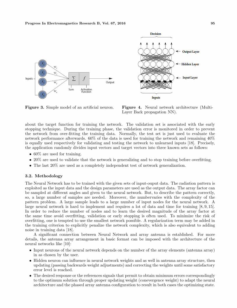
The above Figure 3 represents the simple model of an artificial neuron system that can inspired bybiological nervous systems, such as the brain, process information (see Figure 2) [12, 13]. It is composedof a large number of highly interconnected processing elements (neurons) working in unison to solvespecific problems. Every component of the structure bears a direct analogy to the actual constitutesof a biological neuron and hence it is termed as artificial neuron [9]. In this model which explains andperforms the basis function of artificial neural networks. Here, we consider x1, x2, . . . , xn are the ninputs to the artificial neuron and w1, w2, . . . , wn are the weights associated to the input links.

Figure 2. Biological neuron.

Next, a feedforward neural network that is also known as Multi-Layer Perceptrons (MLP) isestablished with a classification algorithm deduced by the neuronal response. The biological neuronreceives all inputs through the dendrites, sums them and produces an output, if the sum is greater thana threshold value. The input signals are passed on to the cell body. So, the data inputs passes throughthe network, layer by layer, until it received by the soma of the artificial neuron at the outputs:

I = w1x1 + w2x2 + . . . + wnxn =n∑

i=1

wixi (7)

To result the final output y, the sum is passed on to a nonlinear filter known activation function whichreleases the output y.

y = f(I) (8)

where f can be a simple threshold function or a sigmoidal, hyperbolic tangent or radial basis function.In this work, we used Lavenberg-Marquard feed forward back propagation algorithm to train and

simulate the network. Neural networks with back propagation algorithm were used to derive themodels for time-varying positioning error tracking. It is a supervised learning example by which alayered feed forward network with continuously valued processing elements is trained for nonlinearpattern mapping. The difference between the target value and network output propagates backwardduring training to adjust the weights so that the network can occur the matching output pattern whenthe corresponding input pattern values is given. Feed forward back propagation network uses feedforward neuron connections and is trained with supervised back propagation learning rule. Network istrained by providing it with input data (phases, amplitudes, distance. . . etc.) and the correspondingoutput data (8). The objective of training is to modify the biases and weights of the network tominimise the error function and to finish with desired output for all possible values of input feed.After deciding the neural network architecture (see Figure 4) with definite structure the network isready to be trained [12, 13]. Previously, three kinds of data sets (inputs) are used, namely the trainingset, the validation set and the test set. The training set is a set of value which contain information


Figure 3. Simple model of an artificial neuron. Figure 4. Neural network architecture (Multi-Layer Back propagation NN).

about the target function for training the network. The validation set is associated with the earlystopping technique. During the training phase, the validation error is monitored in order to preventthe network from over-fitting the training data. Normally, the test set is just used to evaluate thenetwork performance afterwards. 60% of the data is used for training the network and remaining 40%is equally used respectively for validating and testing the network to unlearned inputs [18]. Precisely,the application randomly divides input vectors and target vectors into three known sets as follows:

• 60% are used for training.• 20% are used to validate that the network is generalizing and to stop training before overfitting.• The last 20% are used as a completely independent test of network generalization.

3.2. Methodology

The Neural Network has to be trained with the given sets of input-ouput data. The radiation pattern isexploited as the input data and the design parameters are used as the output data. The array factor canbe sampled at different angles and given to the neural network. But, to describe the pattern correctly,so, a large number of samples are needed. Moreover, the numbervaries with the complexity of thepattern problem. A large sample leads to a large number of input nodes for the neural network. Alarge neural network is hard to implement and requires a lot of data and time for training [8, 9, 15].In order to reduce the number of nodes and to learn the desired magnitude of the array factor atthe same time avoid overfitting, validation or early stopping is often used. To minimize the risk ofoverfitting, one is tempted to use the smallest network possible. A regularization term may be added inthe training criterion to explicitly penalize the network complexity, which is also equivalent to addingnoise in training data [18].

A significant connection between Neural Network and array antenna is established. For moredetails, the antenna array arrangement in basic format can be imposed with the architecture of theneural networks like [10]:

• Input neurons of the neural network depends on the number of the array elements (antenna array)in as chosen by the user.

• Hidden neuron can influence in neural network weights and as well in antenna array structure, thenupdating (passing backwards weight adjustments) and correcting the weights until some satisfactoryerror level is reached.

• The desired response or the references signals that permit to obtain minimum errors correspondinglyto the optimum solution through proper updating weight (conevergence weight) to adapt the neuralarchitecture and the phased array antenna configuration to result in both cases the optimizing state.


• Output neurons as the output signal from the array factor of antenna structure after optimizationto form desired behavioral pattern with minimum of distortion and noiseless.The Figure 5 presents a comparable diagramm between artificial neural network (ANN) architecture

and phased array antenna structure in form multi-layer propagation network.To check if the neural network can generate the required array pattern and their properties.

The training of the artificial neural network (ANN) models for the synthesis is carried out using the

Figure 5. Block diagram of smart antenna array beamformer.

Table 1. Artificial neural network (ANN) training parameters.

Number of input neurons 1000Number of hidden layers 2

Number of output neurons 1Algorithm lm

Learning rate 0.01Momentum 0.95MSE goal 1e−1

Maximum validation failures 10Minimum performance gradient 1e−5

Initial mu 0.001mu decrease factor 0.1mu increase factor 10

Maximum mu 1e10

Epochs between displays 25Generate command-line output false

Show training GUI trueMaximum time to train in seconds inf

Maximum number of epochs 300Regularization parameter 0.8

Transfer function in hidden layer tan-sigmoid (“tansig”)Transfer function in output layer linear(“purelin”)


Levenberg-Marquardt minimization method (the corresponding Matlab function is “trainlm”). Theaccuracy of the artificial neural network (ANN) models is evaluated by mean sum of squared error(MSE) between the calculated by analytic formula and the predicted values for the training data set.

Table 1 resumes the artificial neural network (ANN) training parameters and architecturalparameters prepared for developing the artificial neural network (ANN) models.

4. RESULTS AND OBSERVATION

4.1. Analytic Results

To simulate circular antenna arrays configuration, it is necessary to consider an array antenna in uniformcircular type that can also have an uniform spacing between elements. The considered elements aretaken to be isotropic sources; so its radiation pattern can be described by its array factor. Startingfrom this known structure, we built respectively a concentric circular shaped extension of multiple ringantenna arrays with the same number of elements and different radii form a concentric circular array.

For the verification and the validation of simulation results, we proposed the patterns which areillustrated in Figure 6 and corresponding to both of cases: one ring array and uniformly excited andequally spaced concentric circular ring array.

The extension of uniform circular kind is more straight forward. Let’s assume we have a concentriccircular antenna array (CCAA) (with multiple concentric circular rings) in the (x, y) plane, withpositions given by: N1 = N2 = N3 = N4 = 12 elements, N0 = 1 central element, R1 = λ, R2 = 2λ,R3 = 3λ, R4 = 4λ. This array is plotted in Figure 7. Also, we simulate the array factor of the proposedconcentric circular antenna grid. The result is presented in the same Figure 7.

For a better understanding of these results, we are proposed to study the resulting array factorresponse with another manner based on the Table 2. As illustrated in the same Table 2, this arrayconfiguration presents a better performance in terms Directivity, HPBW and SLL of the proposedstructure were evaluated at various rings (with the same number of elements). The result shows thatby increasing number of elements, higher values of directivity can be achieved. Similar trends can beobserved in HPBW and SLL. We can notice the reduction in SLL with narrow beamwidth (half powerbeamwidth), but the paid cost is the increase in the aperture compared to uniform circular antennagrid (UCCA).

(a) (b)

Figure 6. (a) (3-D) radiation pattern for an uniform circular antenna (UCA) grid using: N1 = 12elements, R1 = λ. (b) (3-D) radiation pattern for a concentric circular antenna (CCA) grid using:N1 = N2 = 12 elements, N0 = 1 central element, R1 = λ, R2 = 2λ.


-5 0 5-5

-4

-3

-2

-1

0

1

2

3

4

5(2-D) Two-dimensional array antennas: elements arranged in concentric circular antenna grid

-2 -1.5 -1 -0.5 0 0.5 1 1.5 2-180

-160

-140

-120

-100

-80

-60

-40

-20

0

θ (rad)

Nor

mal

ized

arr

ay fa

ctor

(dB

)

The Normalized Array Factor

1 ring2 rings3 rings4 rings

(a) (b)y (x/λ)pos

x

(y/

λ)

pos

Figure 7. (a) (2-D) two-dimensional array antennas: elements arranged in concentric circular antennagrid. (b) The normalized array factor using: N1 = N2 = N3 = N4 = 12 elements, N0 = 1 centralelement, R1 = λ, R2 = 2λ, R3 = 3λ, R4 = 4λ.

Table 2. The performance parameters of the cases presented.

RingsDirectivity

(dB)SLL (dB) HPWB (◦)

Gain-beamwidthproduct (◦)

Peak gain

1 38.1151 −7.9 28.1 337.49 12.0 (10.8 dBi)2 46.7659 −16.7 12.7 1822.29 144.0 (21.6 dBi)3 57.9632 −26.8 7.7 13360.65 1727.4 (32.4 dBi)4 64.9851 −34.7 5.3 109273.69 20721.5 (43.2 dBi)

(a) (b)

Figure 8. (a) The beam pattern in (dB) for a concentric circular antenna grid. (b) (3-D) results ofthe electric field as a function of the θ and φ directions using: N1 = N2 = 12 elements, N0 = 1 centralelement, R1 = λ and R2 = 2λ.


(a) (b)

Figure 9. (a) The beam pattern in (dB) for a concentric circular antenna grid. (b) (3-D) results of theelectric field as a function of the θ and φ directions using: N1 = N2 = N3 = N4 = 12 elements, N0 = 1central element, R1 = λ, R2 = 2λ, R3 = 3λ and R4 = 4λ.

-2 -1.5 -1 -0.5 0 0.5 1 1.5 2-180

-160

-140

-120

-100

-80

-60

-40

-20

0

Nor

mal

ized

Arr

ay F

acto

r (d

B)

The Normalized Array Factor (dB)

θ (rad)

θ = 0o0

θ = 30

θ = 60

θ = 90

o

o

o

0

0

0

Figure 10. The array factor (AF) value in (dB) against θ0 steering direction using: φ0 = 0◦,N1 = N2 = N3 = N4 = 12 elements, N0 = 1 central element, R1 = λ, R2 = 2λ, R3 = 3λ andR4 = 4λ.

To plot the array function expression, we will introduce simplifying variables, u = Kxλ2π =

sin(θ) cos(φ) and v = Kyλ2π = sin(θ) sin(φ). Also, the above variables are often used in plotting two-

dimensional patterns, and are known as directional cosines (or (u, v) space). A plot of the AF above isshown in Figures 8 and 9: As expected, the array is maximum when (u, v) = (0, 0), which correspondsto the desired direction (θ = 0, φ = 0)).

Figures 8 and 9 show a 3-D graph of the propagation of the electric field in the θ and φ directions,for all corresponding CCAA structures.

The same Figures 8 and 9 confirm that the main lobe of radiation pattern is reduced by increasingring number. It is clear from Figure 10 that there is only one maximum that occurs at (θ0, φ0 = 0◦) whilesteering the main beam and does not have any grating lobe at π − θ. Following the Figures 11 and 12,considering the (θ0, φ0 = 0◦) values, radiation properties of a concentric circular array of centrally fedradiators are analyzed that shows its better performance in terms of directivity, gain and also full 360◦azimuth scanning. An advantage of this proposed phased array, compared to other type of array antenna


(a) (b)

Figure 11. (3-D) radiation beam pattern steering of proposed array (concentric circular antenna grid).(a) (φ0 = 0◦, θ0 = 60◦). (b) (φ0 = 60◦, θ0 = 60◦) using: N1 = N2 = 12 elements, N0 = 1 centralelement, R1 = λ and R2 = 2λ.

(a) (b)

Figure 12. (a) The beam pattern in (dB) for a concentric circular antenna grid where (φ0 = 30◦, θ0 =30◦) using: N1 = N2 = N3 = N4 = 12 elements, N0 = 1 central element, R1 = λ, R2 = 2λ, R3 = 3λand R4 = 4λ.

configurations, is that the main beam can be electronically steered for a desired direction. The nextexample given in the Figure 12 illustrates the idea of phase steering. Similary, the example scans themain beam of the array from +30 degrees azimuth, with elevation angle fixed at +30 degrees duringthe scan.


4.2. Artificial Neural Network (ANN) Application

In our application, the desired diagram is specified from a mask, the database contains a whole of dataobtained by simulation with the previous study (analytic solution). In this work, we are interestedto apply only planar array antennas arranged in a concentric circular grid. As mentioned before, theuniform circular array (one ring array) should certainly fellow the same network procedure. After severaltests, an artificial neural network (ANN) with the following geometry (see Figure 1) was retained: Twocommonly used methods applied to overcome over-training problem, i.e., to decide when to stop trainingprocess, are early stopping (ES) and regularization methods. ES is widely used because it is easy tounderstand and implement also it has been reported to be superior to regularization methods. In orderto use the ES method, the available normalized array factor’s data must be divided into three sets, aspresented in the Figure 13:

-2 -1.5 -1 -0.5 0 0.5 1 1.5 2-120

-100

-80

-60

-40

-20

0

Nor

mal

ized

Arr

ay F

acto

r (d

B)

The Normalized Array Factor is data divided into three subsets:Training set, Validation set and Testing set

using: N = N = 12 elements, N = 1 central element, R = λ, R = 2λ

trainvalidatetest

θ (rad)

1 2 0 1 2

Figure 13. The normalized array factor is data divided into three subsets: Training set, Validationset and Testing set. The parameters which chosen to simulate the suggested three-dimensional arrayantennas are: φ = 0 rad, N1 = N2 = 12 elements, N0 = 1 central element, R1 = λ and R2 = 2λ.

-100

-90

-80

-70

-60

-50

-40

-30

-20

-10

0

Nor

mal

ized

Arr

ay F

acto

r (d

B)

The Normalized Array Factor Function Approximation with Early Stopping:Improving Generalization with Early Stopping

Target : analytic solutionWithout Early StoppingWith Early Stopping

-2 -1.5 -1 -0.5 0 0.5 1 1.5 2 θ (rad)

Figure 14. The normalized array factor function approximation with Early Stopping (ES): ImprovingGeneralization with Early Stopping (ES). The parameters which chosen to simulate the suggested Three-dimensional array antennas are: φ = 0 rad, N1 = N2 = 12 elements, N0 = 1 central element, R1 = λand R2 = 2λ.


• Training set, used to determine artificial neural network (ANN) weights.• Validation set, used to check the artificial neural network (ANN) performance and decide when to

stop the training process.• Test set, used to assess performance capabilities of developed artificial neural network (ANN)

model.

A more detailed description of the ES method is graphically illustrated in the Figure 14. Themethodology of ES method can be explained in [18].

From the Figure 14, we can see a good accuracy improvement generalization of the normalizedarray factor with Early Stopping (ES) technique. However, artificial neural network (ANN) based onES method (Network with early stopping) is able to generate very fast the results of synthesis comparingto default artificial neural network (ANN) (Network without early stopping) which needs much moreCPU time and memory. In consequence, Network with ES method can better fit the test data set withless discrepancies, therefore the early stopping feature can be used to prevent over-fitting of networktowards the training data.

4.3. Artificial Neural Network (ANN) Performance

The computer code for training the artificial neural network (ANN) and measuring its performance wasimplemented under MATLAB environment. The network was executed with the set of knowledge basedata of Normalized Array Factor. It shows the over all progress of the network. It clearly indicatesthat the training stops on reaching the maximum validation checks of 10. The number of epoch with12 iterations and the performance (MSE) with 11.1, gradient decent value of 1.79 and mu value of 1.00.

Under training the curve, of the overall progress of the artificial neural network (ANN), indicatesthe 2 layer neural network training state plot for network with 1000 input nodes and 1 output nodes withcombination structure as (1-2-1). The training stops when the validation parameter max fail reachedmaximum 10 validation checks at epoch 12 with the gradient decent value 1.7896 with reasonable Muvalue 1.00 which would cause the convergence of the network fast. Because it could be expected thattoo small Mu value would cause the network to converge too slowly. As seen in Figure 15, the bestvalidation performance is reached at epoch 2 and mean squared error (mse) for testing the data is538.5015. In this example, the result is reasonable because of the following considerations:

• The final mean-square error is small.• The test set error and the validation set error have similar characteristics.• No significant over-fitting has occurred by iteration 3 (where the best validation performance

occurs).

0 2 4 6 8 10 1210-2

10-1

100

101

102

103

104Best Validation Performance is 538.5015 at epoch 2

Mea

n S

quar

ed E

rror

(m

se)

12 Epochs

TrainValidationTestBestGoal

Figure 15. Evaluation of mean squared error.


0 50 100

0

50

100

TargetO

utpu

t~=

0.4*

Tar

get+

9

All: R=0.6949

Y = TFitData

0 50 100

0

50

100

Target

Out

put~

=0.

32*T

arge

t+10

Test: R=0.65444

Y = TFitData

0 50 100

0

50

100

Target

Out

put~

=0.

33*T

arge

t+9.

9

Validation: R=0.65231

Y = TFitData

-40 -20 0 20 40

-40

-20

0

20

40

Target

Out

put~

=0.

99*T

arge

t+0.

15

Training: R=0.99512

Y = TFitData

Figure 16. Regression plot of network.

Table 3. Time consumption learning presented on the overall progress of the artificial neural network(ANN).

Trainingtime consumed by

the algorithm (second)Default training (with levenberg algorithm) 3753.685

Training with early stopping method (using levenberg algorithm) 139.68

The regression analysis was obtained by artificial neural network (ANN) model after the networkconcludes training, testing and validation. In the training window, we can perform a linear regressionbetween the network outputs and the corresponding targets. The following Figure 16 shows the resultsof the regression plot of training, test, validation and over all regression. The small circle shows thedata representation in the model. After the regression plot has been evaluated, it’s important to takeunder consideration and fitting the goodness of the diagnosis of the modelis. As all most approachesused coefficient of determination proof for goodness of fit includes R squared expressed as R2, indicateshow well the data points fit a line or curve. In the below figure the best fit was denoted as straightline.The dotted line presents the outputs equal to targets (Y = T ). The relationship between the outputsand the targets are provided by the Regression (R) value for every network architecture. If R = 1, thisproves the exact linear Relationship (R) between outputs and targets. Practically, the R value wouldtend to obtain rarely a perfect value. From all these graphs, best regression value for validating the datais equal to R = 0.65231, regression value for testing the data is defined as R = 0.65444, regression valuefor training the data is defined as R = 0.99512 and overall regression value is R = 0.6949. This provesthe developed model and the network procedure of training, testing and validation are significantlyvalid [12, 13].

To show the speed of the computation time, the difference consumption time between defaulttraining and training with early stopping method (using levenberg algorithm) is given in the Table 3.It proves that the elapsed time of an early stopping method is less important than the time needed fora default training (without early stopping).


5. CONCLUSION

This article presents the limitation of uniform circular antenna arrays to increase the gain and thedirectivity pattern. To enhance the radiation characteristics, we propose to grow up the array elementsnumbers by introducing a concentric circular antenna configuration. Based on this simple geometry, it’spossible to study other aperiodic (random cases) arrays of various three dimensional (3D) geometries(e.g., conformal phased array antenna). This analyze is necessary starting point for future investigationof neural network solution for irregular antenna array synthesis. The adoption of the early stoppingmethod permits to use neural network with reduced complexity. Network contains as little neurons aspossible. If we are lucky, it will be so flexible that it will be able to train — It is more flexible to overfit.Due to the early stopping technique, the neural network training results in a very important gain in therunning time and the used memory.

For a future work, we suggest to apply the optimisation techniques (genetic, LMS,. . . etc.) inconcentric circular antenna arrays to predict the desired radiation that can be adopted to increase thegain and to scan the range by suppressing sidelobe level (SLL).

REFERENCES

1. Luo, Z., X. He, X. Chen, X. Luo, and X. Li, “Synthesis of thinned concentric circular antenna arraysusing modified TLBO algorithm,” International Journal of Antennas and Propagation, Vol. 2015,9 pages, Article ID 586345, 2015.

2. Albagory, Y. and O. Said, “Optimizing concentric circular antenna arrays for high-altitudeplatforms wireless sensor networks,” I.J. Computer Network and Information Security, Vol. 5,1–8, 2014.

3. Reyna Maldonado, A., M. A. Panduro, and C. del Rio-Bocio, “On the design of concentric ringarray for isoflux radiation in Meo satellites based on PSO,” Progress In Electromagnetics ResearchM, Vol. 20, 243–255, 2011.

4. Reynaa, A., M. A. Panduroa, D. H. Covarrubias, and A. Mendeza, “Design of steerable concentricrings array for low side lobe level,” Scientia Iranica, Vol. 19, No. 3, 727–732, Jun. 2012.

5. Zhang, L., Y.-C. Jiao, and B. Chen, “Optimization of concentric ring array geometry for 3D beamscanning,” International Journal of Antennas and Propagation, Vol. 2012, 5 pages, Article ID625437, 2012.

6. Yan, K.-K. and Y. Lu, “Sidelobe reduction in array-pattern synthesis using genetic algorithm,”IEEE Transactions on Antennas and Propagation, Vol. 45, No. 7, Jul. 1997.

7. Mandal, D., S. P. Ghoshal, and A. K. Bhattacharjee, “Optimized radii and excitations withconcentric circular antenna array for maximum sidelobe level reduction using wavelet mutationbased particle swarm optimization techniques,” Telecommunication Systems, Vol. 52, No. 4, 2015–2025, Apr. 2013.

8. Elsaidy, E. I., M. I. Dessouky, S. Khamis, and Y. A. Albagory, “Concentric circular antenna arraysynthesis using comprehensive learning particle swarm optimizer,” Progress In ElectromagneticsResearch Letters, Vol. 29, 1–13, 2012.

9. Rawata, A., R. N. Yadavb, and S. C. Shrivastavac, “Neural network applications in smart antennaarrays: A review,” AEU — International Journal of Electronics and Communications, Vol. 66,No. 11, 903–912, Nov. 2012.

10. Zaharis, Z. D., K. A. Gotsis, and J. N. Sahalos, “Comparative study of neural network trainingapplied to adaptive beamforming of antenna arrays,” Progress In Electromagnetics Research,Vol. 126, 269–283, 2012.

11. Guo, H., C.-J. Guo, Y. Qu, and J. Ding, “Pattern synthesis of concentric circular antenna array bynonlinear least-square method,” Progress In Electromagnetics Research B, Vol. 50, 331–346, 2013.

12. Dudczyk, J. and A. Kawalec, “Adaptive forming of the beam pattern of microstrip antenna with theuse of an artificial neural network,” International Journal of Antennas and Propagation, Vol. 2012,13 pages, Article ID 935073, 2012.


13. Ali, B. A. A., M. S. Salit, E. S. Zainudin, and M. Othman, “Integration of artificial neural networkand expert system for material classification of natural fibre reinforced polymer composites,”American Journal of Applied Sciences, Vol. 12, No. 3, 174–184, Apr. 2015.

14. Ghayoula, R., N. Fadlallah, A. Gharsallah, and M. Rammal, “Phase-only adaptive nulling withneural networks for antenna array synthesis,” IET Microw. Antennas Propag., Vol. 3, No. 1, 154–163, 2009.

15. Merad, L., F. T. Bendimerad, S. M. Meriah, and S. A. Djennas, “Neural networks for synthesisand optimization of antenna arrays,” Radioengineering, Vol. 16, No. 1, Apr. 2007.

16. Kapetanakis, T. N., I. O. Vardiambasis, G. S. Liodakis, M. P. Ioannidou, and A. M. Maras, “Smartantenna design using neural networks,” 8th International Conference: New Horizons in Industry,Business and Education (NHIBE 2013), 130–135, Chania, Greece, 2013.

17. Pei, B., H. Han, Y. Sheng, and B. Qiu, “Research on smart antenna beamforming bygeneralized regression neural network,” 2013 IEEE International Conference on Signal Processing,Communication and Computing (ICSPCC), 2013.

18. Wang, L., H. C. Quek, K. H. Tee, N. Zhou, and C. Wan, “Optimal size of a feedforwardneural network: How much does it matter?,” Joint International Conference on Autonomic andAutonomous Systems and International Conference on Networking and Services, Papeete, Tahiti,Oct. 23–28, 2005.

uniform and concentric circular antenna arrays synthesis ... · uniform and concentric circular...

Documents